Exact equilibrium properties of square-well and square-shoulder disks in single-file confinement

Abstract

This study investigates the (longitudinal) thermodynamic and structural characteristics of single-file confined square-well and square-shoulder disks by employing a mapping technique that transforms the original system into a one-dimensional polydisperse mixture of nonadditive rods. Leveraging standard statistical-mechanical techniques, exact results are derived for key properties, including the equation of state, internal energy, radial distribution function, and structure factor. The asymptotic behavior of the radial distribution function is explored, revealing structural changes in the spatial correlations. Additionally, exact analytical expressions for the second virial coefficient are presented. Comparisons with Monte Carlo simulations demonstrate an excellent agreement with theory.

I Introduction

The study of thermodynamic and structural properties of liquids whose particles interact via simple pairwise potentials has been a field of interest for many years [1, 2, 3, 4, 5, 6, 7, 8]. The primary rationale behind this focus is the simplicity of such interactions, enabling a profound understanding of system behavior while retaining key realistic features akin to those observed in actual fluids.

Within the realm of these elementary potentials, two that stand out prominently are the square-well (SW) [9, 10, 8, 11, 12] and square-shoulder (SS) [13, 14, 15, 16] potentials. They are characterized by an impenetrable hard core paired with either an attractive well or a repulsive step. The SS potential is purely repulsive and belongs to the family of the so-called core-softened potentials, which have been widely used to study metallic liquids [17] or water anomalies [18, 19, 20, 21, 22]. Conversely, the SW potential comprises a repulsive hard core complemented by an attractive well, making it suitable for modeling more intricate fluids governed by competing interactions [23, 6].

Although fluids of particles interacting with these two potentials have been thoroughly studied using different approaches, to the best of our knowledge, little is still known about their behavior in confined geometries [24, 25]. Confined liquids manifest in diverse scenarios, spanning from biological systems to material science. Unraveling the distinctions in their properties compared to bulk liquids constitutes a pivotal stride toward comprehending their behavior in entirety [26, 27].

This paper focuses on highly confined SW and SS two-dimensional (2D) systems, where the length of one of the dimensions is much larger than that of the other one, the latter being so small as to confine particles into single-file formation. In such a scenario, the system can be treated as quasi one-dimensional (Q1D) [28, 29, 30, 31, 32, 33, 34, 35, 36, 37, 38, 39, 40, 41, 42, 43, 44, 45, 46, 47, 48, 49, 25], and its most relevant properties are the longitudinal ones.

In these circumstances, the advantage of confined SW and SS disks becomes apparent over more intricate potentials. Their properties can be precisely and at times analytically determined by employing a mapping technique that transforms the system into a one-dimensional (1D) polydisperse mixture of nonadditive rods with equal chemical potential [48, 49]. The significance of confined systems with exact solutions is evident, as they not only facilitate a more profound exploration of their physical properties but also serve as a reliable benchmark for assessing the accuracy of approximate methods and computer simulations. This, in turn, enhances their utility in studying more intricate systems [50, 51, 52, 53].

The structure of our paper is the following: Section II describes the confined system, along with its main properties, and establishes the equivalence between the confined system and its 1D mixture counterpart. Section III presents the exact theoretical results for its main (longitudinal) thermodynamic and structural properties and a derivation of the second virial coefficient and the Boyle temperature, while Sec. IV is devoted to a brief description of our own Monte Carlo (MC) simulations. In Sec. V, an analysis of all results is presented, with information on the density profile, the equation of state, the internal energy, the radial distribution function, and the structure factor. Finally, some concluding remarks are provided in Sec. VI.

II The Confined SW and SS Fluids

II.1 The 2D system

We consider a 2D system of $N$ particles interacting via a pairwise potential,

$$\varphi(r)=\begin{cases}\infty&\text{if }r<1\\ -\varphi_{0}&\text{if }1<r<r_{0}\\ 0&\text{if }r>r_{0}\\ \end{cases},$$ (1)

where $r_{0}$ is the range of interaction and, for simplicity, the hard-core diameter of the particles defines the unit of length. The sign of $\varphi_{0}$ determines whether, in addition to the hard core, the potential has an attractive corona ($\varphi_{0}>0$, SW) or a repulsive one ($\varphi_{0}<0$, SS). A schematic representation of both potentials is shown in Fig. 1. The depth of the well ($\varphi_{0}$) or the height of the shoulder ($|\varphi_{0}|$) allows us to define a reduced temperature $T^{*}=k_{B}T/|\varphi_{0}|$, where $T$ is the absolute temperature and $k_{B}$ is the Boltzmann constant.

Figure 1: Schematic representation of (a) the SW potential and (b) the SS potential.

The particles are assumed to be confined in a very long rectangular channel of width $w=1+\epsilon$, where the excess pore width ($\epsilon$) is the available space for the particle centers, and length $L\gg w$. To avoid second-nearest neighbor interactions, for any given value of the corona diameter ($r_{0}$), the maximum value of the excess pore width is limited to $\epsilon_{\mathrm{max}}=\sqrt{1-r_{0}^{2}/4}$, as shown in Fig. 2. Under these conditions, the channel is narrow enough to prevent the particles from bypassing each other, forcing them into a single file. Note also that the particles interact with the walls only through the hard core diameter.

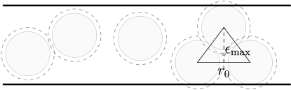
Figure 2: Schematic representation of the particles confined in a narrow channel

In general, if two particles $\alpha$ and $\alpha^{\prime}$ are in close contact (i.e., $r_{\alpha\alpha^{\prime}}=1$) with a transverse separation $|y_{\alpha}-y_{\alpha^{\prime}}|$ between their centers, their longitudinal separation is $|x_{\alpha}-x_{\alpha^{\prime}}|=a(y_{\alpha}-y_{\alpha^{\prime}})$, where

$$a(\Delta y)\equiv\sqrt{1-\Delta y^{2}}.$$ (2)

Similarly, if the coronas of two particles are in contact (i.e., $r_{\alpha\alpha^{\prime}}=r_{0}$), then $|x_{\alpha}-x_{\alpha^{\prime}}|=b(y_{\alpha}-y_{\alpha^{\prime}})$, where

$$b(\Delta y)\equiv\sqrt{r_{0}^{2}-\Delta y^{2}}.$$ (3)

Due to the high anisotropy between the transverse and longitudinal directions of this system, it is often useful to focus on its longitudinal properties, such as the number of particles per unit length, $\lambda\equiv N/L$, the longitudinal pressure $P_{\|}$ and the reduced pressure $p=wP_{\|}$. Note that there exists a close-packing density $\lambda_{\text{cp}}=1/a(\epsilon)$ at which pressure diverges.

For a given corona diameter $r_{0}$, the control parameters can be chosen as the excess pore width $\epsilon$, the reduced temperature $T^{*}$, and the linear density $\lambda$ (or, equivalently, the product $\beta p$, where $\beta\equiv 1/k_{B}T$). In the high-temperature limit ($T^{*}\to\infty$), the attractive or repulsive corona becomes irrelevant and thus the system reduces to a pure hard-disk (HD) one, which has been well studied [28, 29, 30, 31, 32, 33, 34, 35, 36, 37, 38, 39, 40, 41, 42, 43, 44, 45, 46, 47, 48, 49]. To make this property more explicit, suppose that $X$ is a quantity of dimensions (length)^m; then,

$$\lim_{T^{*}\to\infty}X^{\text{SW}}(\lambda,T^{*};r_{0},\epsilon)= \lim_{T^{*}\to\infty}X^{\text{SS}}(\lambda,T^{*};r_{0},\epsilon)$$

$$= X^{\text{HD}}(\lambda;\epsilon).$$ (4)

In the opposite low-density limit ($T^{*}\to 0$), the SS particles become equivalent to HDs of diameter $r_{0}$; therefore,

$$\lim_{T^{*}\to 0}X^{\text{SS}}(\lambda,T^{*};r_{0},\epsilon)=r_{0}^{m}X^{\text{HD}}(\lambda r_{0};\epsilon/r_{0}).$$ (5)

II.2 Equivalent 1D system

It can be shown that the longitudinal properties of the confined 2D system described in Sec. I can be exactly matched to those of an equivalent 1D polydisperse mixture, where the transverse coordinate of each particle,$-\epsilon/2<y<\epsilon/2$, plays the role of the dispersity parameter, and where the chemical potential of all components of the mixture is the same. While the original application of this equivalence was in the context of a HD fluid [48, 49], it can be readily extended to any interaction potential $\varphi(r)$, with the caveat that interactions are constrained to nearest neighbors.

Although the equivalence holds precisely when the 1D mixture features a continuous distribution of components, practical considerations often demand the discretization of the system for numerical computations. Therefore, it usually proves more pragmatic to examine a 1D mixture with a discrete but adequately large number of components, $M$, to accurately characterize the system. The theoretical expressions valid for the original continuous case can then be derived by considering the limit $M\to\infty$.

In this discrete $M$-component mixture, each 1D component, indexed as $i=1,2,\ldots,M$, corresponds to a mapping of 2D particles with a transverse coordinate

$$y_{i}=-\frac{\epsilon}{2}+(i-1)\delta y,\quad\delta y\equiv\frac{\epsilon}{M-1}.$$ (6)

In turn, the 2D interaction potential $\varphi(r)$ translates into the 1D potential

$$\varphi_{ij}(x)= \varphi\left(\sqrt{x^{2}+(y_{i}-y_{j})^{2}}\right)$$

$$= \begin{cases}\infty&\text{if }x<a_{ij}\\ -\varphi_{0}&\text{if }a_{ij}<x<b_{ij}\\ 0&\text{if }x>b_{ij}\end{cases},$$ (7)

where

$$a_{ij}\equiv a(y_{i}-y_{j}),\quad b_{ij}\equiv b(y_{i}-y_{j}).$$ (8a)

Within this framework, one can precisely ascertain the properties of the 1D mixture and directly map them back onto the original 2D system.

III Exact solution

Most of the properties of 1D mixtures are derived in the isothermal-isobaric ensemble and can be described through the Laplace transform of the Boltzmann factor [54],

$$\Omega_{ij}(s,\beta)=\int_{0}^{\infty}{d}x\,e^{-sx}e^{-\beta\varphi_{ij}(x)},$$ (9)

which, in the case of the 1D mixture at hand, yields

$$\Omega_{ij}(s,\beta)=\frac{e^{\beta^{*}}}{s}\left[e^{-a_{ij}s}-\left(1-e^{-\beta^{*}}\right)e^{-b_{ij}s}\right].$$ (10)

Here, $\beta^{*}\equiv\beta\varphi_{0}$. Note that $\beta^{*}=1/T^{*}$ and $\beta^{*}=-1/T^{*}$ for SW and SS, respectively.

In the standard theory of liquid mixtures, mole fractions are considered pre-determined thermodynamic variables. Yet, in the 1D mixture under consideration, the requirement for identical chemical potentials imposes specific conditions on the values of the mole fractions for each component. Let $\phi_{i}^{2}$ denote the mole fraction of component $i$. Then, the set $\{\phi_{i}\}$ is obtained by solving the eigenvalue equation

$$\sum_{j}\Omega_{ij}(\beta p,\beta)\phi_{j}=\frac{1}{A^{2}}\phi_{i},$$ (11)

where $A$ is a constant directly related to the chemical potential as $\beta\mu=\ln(A^{2}\Lambda_{\mathrm{dB}})$, $\Lambda_{\mathrm{dB}}$ being the thermal de Broglie wavelength.

III.1 Thermodynamic properties

Two of the paramount thermodynamic quantities essential for computation in any equilibrium system are the equation of state and the excess internal energy per particle. The equation of state establishes a connection between pressure, density, and temperature, while the excess internal energy per particle encompasses the potential energy per particle (which, combined with the ideal-gas kinetic energy $u_{\mathrm{id}}=k_{B}T$, contributes to the overall internal energy per particle).

In general terms, the compressibility factor, $Z\equiv\beta p/\lambda$, and the excess internal energy per particle, $u_{\mathrm{ex}}$, of any given 1D mixture with equal chemical potentials are given by

$$Z=-A^{2}\beta p\sum_{i,j}\phi_{i}\phi_{j}\left[\frac{\partial\Omega_{ij}(\beta p,\beta)}{\partial\beta p}\right]_{\beta},$$ (12a)

$$u_{\mathrm{ex}}=-A^{2}\sum_{i,j}\phi_{i}\phi_{j}\left[\frac{\partial\Omega_{ij}(\beta p,\beta)}{\partial\beta}\right]_{\beta p}.$$ (12b)

Using Eq. (10), Eqs. (12) become

$$Z=1+A^{2}e^{\beta^{*}}\sum_{i,j}\phi_{i}\phi_{j}\left[a_{ij}e^{-\beta pa_{ij}}-b_{ij}\left(1-e^{-\beta^{*}}\right)e^{-\beta pb_{ij}}\right],$$ (13a)

$$\frac{u_{\text{ex}}}{\varphi_{0}}=-1+\frac{A^{2}}{\beta p}\sum_{i,j}\phi_{i}\phi_{j}e^{-\beta pb_{ij}},$$ (13b)

where we have used Eq. (11) and the normalization condition $\sum_{i}\phi_{i}^{2}=1$.

III.2 Structural properties

Contrary to the thermodynamic properties, which are related to global quantities of the system, structural properties are mainly related to the arrangements of the particles and the different configurations they are placed into. The basic structural property that can be looked into is the (longitudinal) radial distribution function (RDF) $g_{ij}(x)$ which, in Laplace space, is given by [49]

$$\widetilde{G}_{ij}(s)= \int_{0}^{\infty}dx\,e^{-sx}g_{ij}(x)$$

$$= \frac{A^{2}}{\lambda\phi_{i}\phi_{j}}\left[\mathsf{\Omega}(s+\beta p)\cdot\left[\mathsf{I}-A^{2}\mathsf{\Omega}(s+\beta p)\right]^{-1}\right]_{ij},$$ (14)

where $\mathsf{\Omega}$ is the $M\times M$ matrix of elements $\Omega_{ij}$ and $\mathsf{I}$ is the unit matrix. Henceforth, for enhanced clarity, we will omit the second argument ($\beta$) in $\Omega_{ij}$.

The RDF in real space can be obtained by performing the inverse Laplace transform on Eq. (III.2). The structure of the analytical form of $g_{ij}(x)$ is presented in Appendix A. At a practical level, we have used Eq. (37) for $x\leq 3a(\epsilon)$. For larger distances, it is preferable to invert $\widetilde{G}_{ij}(s)$ numerically [55]. Once the partial RDFs $g_{ij}(x)$ are known, the total RDF is obtained as

$${g}(x)=\sum_{i,j}\phi_{i}^{2}\phi_{j}^{2}{g}_{ij}(x).$$ (15)

The structure factor is another pivotal quantity that, although conveying the same physical information as the RDF, can be experimentally accessed through diffraction experiments. The 1D structure factor is directly linked to the Fourier transform of the total correlation function $h(x)\equiv g(x)-1$,

$$S(q)=1+2\lambda\int_{0}^{\infty}{d}x\cos(qx)h(x).$$ (16)

In our scheme, this is equivalent to

$$S(q)=1+\lambda\left[\widetilde{G}(s)+\widetilde{G}(-s)\right]_{s=\imath q},$$ (17)

where $\widetilde{G}(s)=\sum_{i,j}\phi_{i}^{2}\phi_{j}^{2}\widetilde{G}_{ij}(s)$ and $\imath$ is the imaginary unit.

III.3 Compressibility factor in terms of the RDF

For an arbitrary (nearest-neighbor) interaction potential $\varphi_{ij}(x)$, the compressibility factor $Z$ is given by Eq. (12a), while the RDF $g(x)$ is given by Eqs. (III.2) and (15). In both cases one first needs to evaluate the Laplace transform $\Omega_{ij}(s)$. The interesting question is, can one express $Z$ directly in terms of density and integrals involving $g(x)$? An affirmative response can be found in Appendix B, with the outcome

$$Z=\frac{1-\lambda\int_{a(\epsilon)}^{r_{0}}dx\,g(x)}{1-\lambda\left[r_{0}-\lambda\int_{a(\epsilon)}^{r_{0}}dx\,(r_{0}-x)g(x)\right]},$$ (18)

Equation (18) generalizes Eq. (2.13) of Ref. [25] and can be conveniently employed in NVT simulations.

III.4 Continuous polydisperse mixture

To take the continuum limit, let us define the transverse density profile of the original 2D system by $\phi^{2}(y_{i})=\phi_{i}^{2}/\delta y$, as well as the parameter $\ell=(\beta p/A^{2})\delta y$. Also, Eq. (10) can be written as

$$\Omega(y,y^{\prime};s)=\frac{e^{\beta^{*}}}{s}\left[e^{-a(y-y^{\prime})s}-\left(1-e^{-\beta^{*}}\right)e^{-b(y-y^{\prime})s}\right].$$ (19)

Now, taking the limit $M\to\infty$ (which implies $\delta y\to 0$), Eqs. (11) and (13) become

$$\int_{-\frac{\epsilon}{2}}^{\frac{\epsilon}{2}}dy^{\prime}\,\Omega(y,y^{\prime};\beta p)\phi(y^{\prime})=\frac{\ell}{\beta p}\phi(y),$$ (20a)

$$Z= 1+\frac{\beta p}{\ell}e^{\beta^{*}}\int_{-\frac{\epsilon}{2}}^{\frac{\epsilon}{2}}dy\int_{-\frac{\epsilon}{2}}^{\frac{\epsilon}{2}}dy^{\prime}\,\left[a(y-y^{\prime})e^{-\beta pa(y-y^{\prime})}\right.$$

$$\left.-b(y-y^{\prime})\left(1-e^{-\beta^{*}}\right)e^{-\beta pb(y-y^{\prime})}\right]\phi(y)\phi(y^{\prime}),$$ (20b)

$$\frac{u_{\text{ex}}}{\varphi_{0}}=-1+\frac{1}{\ell}\int_{-\frac{\epsilon}{2}}^{\frac{\epsilon}{2}}dy\int_{-\frac{\epsilon}{2}}^{\frac{\epsilon}{2}}dy^{\prime}\,e^{-\beta pb(y-y^{\prime})}\phi(y)\phi(y^{\prime}).$$ (20c)

In what concerns the structural properties, let us first rewrite Eq. (III.2) in the equivalent form

$$\frac{\phi_{j}\widetilde{G}_{ij}(s)}{A^{2}}=\frac{\Omega_{ij}(s+\beta p)}{\lambda\phi_{i}}+\sum_{k}\phi_{k}\widetilde{G}_{ik}(s)\Omega_{kj}(s+\beta p),$$ (21)

and define $g(y_{i},y_{j};x)=g_{ij}(x)$ in real space and $\widetilde{G}(y_{i},y_{j};s)=\widetilde{G}_{ij}(s)$ in Laplace space. Then, in the limit $M\to\infty$ we get the following linear integral equation of the second kind,

$$\frac{\ell\phi(y^{\prime})\widetilde{G}(y,y^{\prime};s)}{\beta p}= \frac{\Omega(y,y;s+\beta p)}{\lambda\phi(y)}+\int_{-\frac{\epsilon}{2}}^{\frac{\epsilon}{2}}dy^{\prime\prime}\,\phi(y^{\prime\prime})$$

$$\times\widetilde{G}(y,y^{\prime\prime};s)\Omega(y^{\prime\prime},y^{\prime};s+\beta p).$$ (22)

In turn, Eq. (15) becomes

$$g(x)=\int_{-\frac{\epsilon}{2}}^{\frac{\epsilon}{2}}dy\int_{-\frac{\epsilon}{2}}^{\frac{\epsilon}{2}}dy^{\prime}\,\phi^{2}(y)\phi^{2}(y^{\prime})g(y,y^{\prime};x).$$ (23)

Note that Eq. (18) is still applicable in the continuum limit.

III.5 Asymptotic behavior of the RDF

The asymptotic behavior of $g(y,y^{\prime};x)$ is related to the nonzero poles, $\{s_{n}\}$, of $\widetilde{G}(y,y^{\prime};s)$ and their associated residues. In general,

$$g(y,y^{\prime};x)=1+\sum_{n=1}^{\infty}\mathcal{A}_{n}(y,y^{\prime})e^{s_{n}x},$$ (24a)

$$\mathcal{A}_{n}(y,y^{\prime})\equiv \,\mathrm{Res}[\widetilde{G}(y,y^{\prime};s)]_{s_{n}}$$

$$= \left[\frac{\partial}{\partial s}\frac{1}{\widetilde{G}(y,y^{\prime};s)}\right]_{s=s_{n}}^{-1}.$$ (24b)

The asymptotic decay of the total correlation function $h(y,y^{\prime};x)\equiv g(y,y^{\prime};x)-1$ is then determined by either the nonzero real pole $s=-\kappa$ or the pair of conjugate poles $-\kappa\pm\imath\omega$ with the smallest value of $\kappa$. In this framework, $\kappa^{-1}$ represents the longitudinal correlation length and (if the dominant poles are complex) $\omega$ represents the asymptotic oscillation frequency. If $\omega\neq 0$, one has

$$h(y,y^{\prime};x)\approx 2|\mathcal{A}(y,y^{\prime})|e^{-\kappa x}\cos(\omega x+\delta),$$ (25)

for asymptotically large values of $x$, where $\mathcal{A}(y,y^{\prime})=|\mathcal{A}(y,y^{\prime})|e^{\pm\imath\delta}$ is the complex residue. Equation (25) describes an oscillatory decay of $h(y,y^{\prime};x)$. If, on the other hand, the dominant pole is real (i.e., $\omega=0$), then

$$h(y,y^{\prime};x)\approx\mathcal{A}(y,y^{\prime})e^{-\kappa x},$$ (26)

where the residue $\mathcal{A}(y,y^{\prime})$ is also a real number and therefore the asymptotic decay is purely monotonic.

III.6 Second virial coefficient

In the low-density (or low-pressure) regime, the compressibility factor can be expressed as

$$Z= 1+B_{2}\lambda+\mathcal{O}(\lambda^{2})$$

$$= 1+B_{2}\beta p+\mathcal{O}(\beta p^{2}),$$ (27)

where $B_{2}$ is the second virial coefficient.

In general, the behavior of $\Omega(y,y^{\prime};s)$ for small $s$ is of the form

$$\Omega(y,y^{\prime};s)=s^{-1}+\Psi(y,y^{\prime})+\mathcal{O}(s),$$ (28)

where $\Psi(y,y^{\prime})$ does not need to be specified at this stage. By following steps analogous to those in Appendix B of Ref. [48], one can prove that the low-pressure solution to the eigenvalue problem in Eq. (20a) is

$$\phi(y)=\frac{1}{\sqrt{\epsilon}}\left[1+\overline{\phi}_{1}(y)\beta p+\mathcal{O}(\beta p^{2})\right],$$ (29a)

$$\ell=\epsilon\left[1-B_{2}\beta p+\mathcal{O}(\beta p^{2})\right],$$ (29b)

where

$$\overline{\phi}_{1}(y)=B_{2}+\frac{1}{\epsilon}\int_{-\frac{\epsilon}{2}}^{\frac{\epsilon}{2}}dy^{\prime}\,\Psi(y,y^{\prime}),$$ (30a)

$$B_{2}=-\frac{1}{\epsilon^{2}}\int_{-\frac{\epsilon}{2}}^{\frac{\epsilon}{2}}dy\int_{-\frac{\epsilon}{2}}^{\frac{\epsilon}{2}}dy^{\prime}\,\Psi(y,y^{\prime}).$$ (30b)

In the particular case of the SW or SS potentials, from Eq. (19) we can easily identify the function $\Psi(y,y^{\prime})$ as

$$\Psi(y,y^{\prime})=-e^{\beta^{*}}a(y-y^{\prime})+\left(e^{\beta^{*}}-1\right)b(y-y^{\prime}).$$ (31)

Insertion into Eq. (30b) yields

$$B_{2}(T^{*};r_{0},\epsilon)=e^{\beta^{*}}B_{2}^{\text{HD}}(\epsilon)-\left(e^{\beta^{*}}-1\right)r_{0}B_{2}^{\text{HD}}(\epsilon/r_{0}),$$ (32)

where

$$B_{2}^{\text{HD}}(\epsilon)=\frac{2}{3}\frac{\left(1+\frac{\epsilon^{2}}{2}\right)\sqrt{1-\epsilon^{2}}-1}{\epsilon^{2}}+\frac{\sin^{-1}(\epsilon)}{\epsilon}$$ (33)

is the second virial coefficient of the confined HD fluid. As expected from Eqs. (II.1) and (5), $\lim_{T^{*}\to\infty}B_{2}^{\text{SW}}(T^{*};r_{0},\epsilon)=\lim_{T^{*}\to\infty}B_{2}^{\text{SS}}(T^{*};r_{0},\epsilon)=B_{2}^{\text{HD}}(\epsilon)$ and $\lim_{T^{*}\to 0}B_{2}^{\text{SS}}(T^{*};r_{0},\epsilon)=r_{0}B_{2}^{\text{HD}}(\epsilon/r_{0})$.

In the SS case ($\beta^{*}<0$), the second virial coefficient is positive definite. However, in the SW case ($\beta^{*}>0$), it changes from negative to positive values as temperature increases; the temperature at which $B_{2}^{\text{SW}}=0$ defines the Boyle temperature

$$T^{*}_{\text{B}}=-\frac{1}{\ln\left[1-B_{2}^{\text{HD}}(\epsilon)/r_{0}B_{2}^{\text{HD}}(\epsilon/r_{0})\right]}.$$ (34)

At fixed $r_{0}$, $T^{*}_{\text{B}}$ increases as $\epsilon$ increases from $\epsilon=0$ to $\epsilon=\epsilon_{\max}=\sqrt{1-r_{0}^{2}/4}$.

IV Monte Carlo simulations

To test the theoretical results presented in Sec. III for the thermodynamic properties (compressibility factor and internal energy), we have performed isothermal-isobaric (NPT) MC simulations on the original 2D confined system, in which the excess pore width $\epsilon$ and the longitudinal pressure $p$ are kept fixed but the longitudinal length $L$ fluctuates. For the investigation of structural properties, we found it more convenient to employ canonical (NVT) MC simulations.

We have checked the equivalence of results between the NVT and NPT ensembles for both thermodynamic and structural properties, as well as the consistency with the NVT MC data reported in Ref. [25]. Whereas NVT simulations do not provide direct access to the equation of state, the compressibility factor can be computed from $g(x)$ through Eq. (18). Nevertheless, from a practical point of view, the values of $Z$ computed in this manner for large densities become extremely sensitive to numerical errors in the evaluation of the integrals $\int_{a(\epsilon)}^{r_{0}}dx\,g(x)$ and $\int_{a(\epsilon)}^{r_{0}}dx\,(r_{0}-x)g(x)$ [25], which makes the NPT ensemble much more suitable to compute the equation of state.

In general, $10^{7}$ samples were collected from a system with $10^{2}$ particles, after an equilibration process of at least $10^{7}$ configurations and with an acceptance ratio of roughly $50\%$.

V Results

As shown in Sec. II.1, a SW or SS interaction potential of range $r_{0}$ sets the maximum value of the excess pore width to $\epsilon_{\mathrm{max}}=\sqrt{1-r_{0}^{2}/4}$. The two limiting cases for these values correspond to the pure 1D system ($r_{0}=2,\,\epsilon=0$) and to the confined HD fluid ($r_{0}=1,\,\epsilon=\sqrt{3}/2\simeq 0.866$), both of them already studied exactly in the literature [56, 32, 54, 48, 49].

As a compromise between introducing a nonnegligible corona and, at the same time, departing from the pure 1D system, we have chosen the values $r_{0}=1.2$ and $\epsilon=\epsilon_{\mathrm{max}}=0.8$, in which case $\lambda_{\text{cp}}\simeq 1.67$. The open-source C++ code employed to obtain the results in this section is available for access through Ref. [57].

An observation is worth mentioning. When delving into the theoretical expressions presented in Secs. III.1 and III.2, it becomes imperative to assign a finite value to $M$. As emphasized in Ref. [48], opting for $M=251$ typically proves sufficiently large to render finite-$M$ effects practically negligible. Conversely, in order to eliminate any potential impact of a finite $M$, we systematically computed the relevant quantities for various $M$ values (specifically, $M=51,101,151,201,251$), modeled them as linear functions of $1/M$, and ultimately approached the limit $1/M\to 0$ in the extrapolations. This procedure is illustrated in Fig. 3 for $Z$ and $g(1)$ at $T^{*}=1$ and $5$ with $\lambda=1$. As observed, the local values of the RDF are notably more sensitive to finite $M$ than the thermodynamic quantities.

Figure 3: Plot of (a) $Z$ and (b) $g(1)$ versus $1/M$ for $T^{*}=1$ (circles) and $T^{*}=5$ (squares), in both cases with $\lambda=1$. The lines (solid for SW and dashed for SS) are linear fits to the numerical data. The open symbols at $1/M$ denote the extrapolations to $M\to\infty$.

V.1 Transverse density profile

The transverse density profile $\phi^{2}(y)$, computed from Eq. (20a), is shown in Fig. 4 for both potentials at different densities and temperatures. In general, the density profile tends to be uniform at low densities, but becomes more abrupt, with more particles near the walls and fewer in the center of the pore, as the density increases. As close packing is approached, all particles tend to arrange in a zigzag configuration at both the top and bottom of the channel. Figure 4(a) shows that, at low temperatures and medium or high densities, the profiles are much more abrupt in the case of the SS potential, where the excluded volume effects are more dominant. At high temperatures, however, SW and SS fluids are nearly equivalent, as both behave essentially like HD fluids.

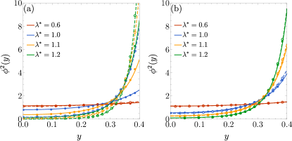
Figure 4: Density profile at different densities for (a) $T^{*}=0.3$ and (b) $T^{*}=5.0$ for the SW (solid lines) and the SS (dashed lines) systems. The symbols (closed for SW, open for SS) are MC simulation results.

V.2 Equation of state and excess internal energy

The compressibility factor, Eq (20), for different temperature values is shown in Fig. 5(a). In the SW case, due to the attractive part of the potential, there exists a range of temperatures, $0<T^{*}<T_{\mathrm{B}}^{*}\simeq 0.59$ [see Eq. (34)], for which $Z<1$ at low densities, whereas $Z>1$ is always fulfilled for every value of temperature and density in the SS case.

In agreement with Eq. (II.1), in the limit $T^{*}\rightarrow\infty$, both SW and SS fluids recover the equation of state of a confined HD fluid of unit diameter and pore width $\epsilon=0.8$, as can be observed in Fig. 5(a). We have also checked that, in agreement with Eq. (5), in the SS case at low temperatures, $T^{*}\rightarrow 0$, we also recover the solution of a confined HD system, where the disks have a hard-core diameter $r_{0}=1.2$, the pore width is $\epsilon/r_{0}\simeq 0.67$, and the density is $r_{0}\lambda=1.2\lambda$. Interestingly, at high densities and a nonzero temperature, the compressibility factor of both systems tends to that of a HD fluid, with $Z$ diverging at $\lambda=\lambda_{\text{cp}}\simeq 1.67$.

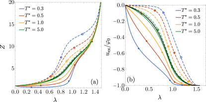
Figure 5: (a) Compressibility factor and (b) excess internal energy as functions of density at different representative temperatures for SW (solid lines) and SS (dashed lines) potentials. The solid black lines represents the limit at infinite temperature (HD fluid), while symbols represent MC simulation results.

The excess internal energy per particle, as derived from Eq. (20c), is shown in Fig. 5(b) in units of $\varphi_{0}$ for both the SW potential, where $u_{\text{ex}}$ is always negative due to the attractive well ($\varphi_{0}>0$), and for the SS potential, where it is always positive ($\varphi_{0}<0$). As density increases, $u_{\text{ex}}/\varphi_{0}$ tends to $-1$ since the coronas of neighbor particles are overlapped in the high-density regime. This effect is more pronounced for lower temperatures in the SW case. In contrast, it is more accentuated for higher temperatures in the SS case because overpassing the repulsive barrier requires high enough temperatures. The solid black line in Fig. 5(b) actually represents a nominal excess energy for a HD fluid since it is obtained from Eq. (20c) by using the HD eigenvalue $\ell$ and eigenfunction $\phi(y)$, even though $b(\Delta y)$ keeps being defined by Eq. (3).

Figure 6: Total RDF for the SW fluid at different temperatures for several values of density: (a) $\lambda=0.6$, (b) $\lambda=1.0$, (c) $\lambda=1.1$, and (d) $\lambda=1.2$. Symbols are MC simulation results.

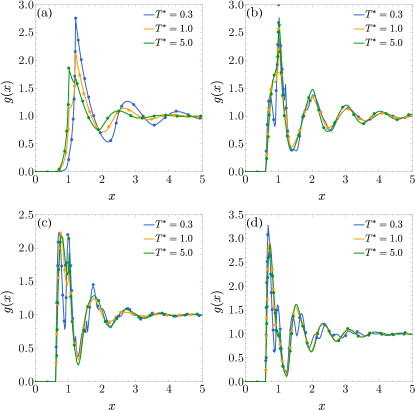
Figure 7: Total RDF for the SS fluid at different temperatures for several values of density: (a) $\lambda=0.6$, (b) $\lambda=1.0$, (c) $\lambda=1.1$, and (d) $\lambda=1.2$. Symbols are MC simulation results.

V.3 Radial distribution function

V.3.1 Total RDF

The RDF is one of the most important structural quantities of any system, since it measures how local density varies with distance from a reference particle with respect to the density of the ideal gas.

In Fig. 6, the total RDF for the SW potential is illustrated across varying densities and temperatures. Notably, at lower densities, temperature emerges as a key factor influencing the amplitude of the oscillations. However, this dependency diminishes substantially at higher densities, where the RDF undergoes minimal alteration with temperature variations, resembling closely the RDF of the HD fluid at equivalent density. The positions of the minima and maxima are notably influenced by density but exhibit minimal sensitivity to temperature changes. Specifically, our observations indicate that the first peak occurs around $x=1$ at $\lambda=0.6$ and $\lambda=1.0$, while a local maximum emerges near $x=a(\epsilon)=0.6$ at $\lambda=1.1$. Notably, this local maximum becomes the absolute maximum at $\lambda=1.2$.

For the SS potential, the RDF is presented in Fig. 7, with the same densities and temperatures as depicted in Fig. 6. Due to the repulsive nature of the potential, temperature plays a larger role in the position of the peaks than in the SW case, especially at low densities, where the first peak shifts from $x=r_{0}=1.2$ to $x=1.0$ with increasing temperature. At higher densities, lower temperatures result in a significantly less ordered structure.

V.3.2 Partial RDFs

In contrast to the total RDF, partial RDFs describe spatial correlations between particles at fixed transverse coordinates. Out of all possible partial RDFs, $g(y,y^{\prime};x)$, the most interesting ones correspond to $y,y^{\prime}=\pm\frac{\epsilon}{2}$, that is,

$$g_{++}(x)\equiv g\left(\frac{\epsilon}{2},\frac{\epsilon}{2};x\right)=g\left(-\frac{\epsilon}{2},-\frac{\epsilon}{2};x\right),$$ (35a)

$$g_{+-}(x)\equiv g\left(\frac{\epsilon}{2},-\frac{\epsilon}{2};x\right)=g\left(-\frac{\epsilon}{2},\frac{\epsilon}{2};x\right).$$ (35b)

While $g_{++}(x)$ encodes spatial correlations between two particles that are both in the top (or bottom) part of the channel, $g_{+-}(x)$ measures spatial correlations of a particle in contact with one of the walls with respect to a particle in contact with the opposite wall. Note that near close packing, all particles are very close to the walls, so that $g(x)\simeq\frac{1}{2}[g_{++}(x)+g_{+-}(x)]$.

Figures 8 and 9 show $g_{++}(x)$ and $g_{+-}(x)$ for the SW and SS potentials, respectively, at the same temperatures and densities as in Figs. 6 and 7. In both classes of potentials, $g_{++}(x)=0$ if $x<1$ and $g_{+-}(x)=0$ if $x<a(\epsilon)=0.6$, as expected. Also in both cases, the disappearance of the peak in $g_{++}(1^{+})$ when density is increased is directly related to the disappearance of defects in the zigzag structure that arises in the close-packing configuration [49].

Figure 8: Partial RDFs $g_{++}(x)$ (solid lines) and $g_{+-}(x)$ (dashed lines) for the SW fluid at different temperatures for several values of density: (a) $\lambda=0.6$, (b) $\lambda=1.0$, (c) $\lambda=1.1$, and (d) $\lambda=1.2$. Symbols are MC simulation results.

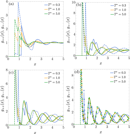
Figure 9: Partial RDFs $g_{++}(x)$ (solid lines) and $g_{+-}(x)$ (dashed lines) for the SS fluid at different temperatures for several values of density: (a) $\lambda=0.6$, (b) $\lambda=1.0$, (c) $\lambda=1.1$, and (d) $\lambda=1.2$. Symbols are MC simulation results.

Figure 10: Plot of (a) the inverse correlation length and (b) the oscillation frequency as functions of density at different temperatures for the SW fluid.

Figure 11: Plot of (a) the inverse correlation length and (b) the oscillation frequency as functions of density at different temperatures for the SS fluid.

V.3.3 Asymptotic behavior

As elaborated in Sec. III.5, the large-$x$ asymptotic behavior of the RDF is determined by the dominant poles of $\widetilde{G}(y,y^{\prime};s)$. To obtain them, we have started from the discrete version with finite $M$ [see Eq. (III.2)] and found the zeros of $\det\left[\mathsf{I}-A^{2}\mathsf{\Omega}(s+\beta p)\right]$ closest to the imaginary axis. Then, the limit $M\to\infty$ was taken by following the extrapolation method illustrated in Fig. 3.

Figures 10 and 11 show the evolution of the values of $\kappa$ and $\omega$ associated with the leading pole as functions of density. The inverse correlation length, $\kappa$, is always continuous but the oscillation frequency, $\omega$, does present discontinuous jumps that correspond to structural changes. In the case of the SW potential [see Fig. 10(b)], as density increases for very low temperatures ($T^{*}=0.1$ and $0.3$), a first discontinuous jump from $\omega=0$ to $\omega\neq 0$ represents a transition from monotonic to oscillatory decay of $h(y,y^{\prime};x)$ [see Eqs. (26) and (25)]. Although not apparent on the scale of Fig. 10(b), this transition persists at very low densities for higher temperatures (e.g., $T^{*}=1$ and $T^{*}=5$) in the case of the SW fluid. However, it is absent for any temperature in the SS fluid. On the other hand, a jump from a higher frequency to a smaller nonzero frequency takes place at $\lambda\approx 1$ for any temperature and both types of interaction. The abrupt shifts in $\omega$ stem from the crossing of two competing poles sharing identical real parts, leading to distinctive kinks in $\kappa$.

Figure 12: Phase diagram for the SW fluid on the plane $T^{*}$ vs $\lambda$. The circles represent the states considered in Fig. 13.

The phase diagram illustrating the types of asymptotic decay of $h(y,y^{\prime};x)$ for the SW fluid is presented in Fig. 12. Three distinct regions can be discerned on the $T^{*}$ vs $\lambda$ plane. For densities less than $\lambda\simeq 0.9612$ and sufficiently low temperatures, the decay is exclusively monotonic, owing to the prevailing influence of the attractive part of the interaction potential. This region is demarcated from the oscillatory decay region by the Fisher–Widom line [56]. Subsequently, the oscillatory decay region is partitioned into two subregions by a crossover line [58]. Upon traversing this crossover line with increasing density, the oscillation frequency undergoes an abrupt transition from a value $\omega\approx 2\pi\simeq 6.3$ (oscillatory region I) to a smaller value $\omega\approx 4$ (oscillatory region II), mirroring the behavior observed in the HD case [49].

Figure 13: Plot of $h_{++}(x)$ for the SW fluid with $T^{*}=0.1$ and (a) $\lambda=0.5$, (b) $\lambda=1.05$, and (c) $\lambda=1.15$ (see circles in Fig. 12). The solid lines correspond to the full functions, while the dashed lines represent the asymptotic behaviors [see Eqs. (25) and (26)].

Figure 14: Structural crossover lines delineating transitions between two distinct oscillation frequencies (oscillatory regions I and II) are depicted for the SW fluid (right curve) and SS fluid (left curve). The dashed and dash-dotted vertical lines indicate the crossover densities at $\lambda=1.016$ and $\lambda=1.060/r_{0}=0.883$, respectively, corresponding to two confined HD fluids: HD (1), characterized by a hard-core diameter of $1$ and an excess pore width of $\epsilon=0.8$, and HD ($r_{0}$), with a diameter of $r_{0}=1.2$ and an excess pore width $\epsilon/r_{0}\simeq 0.67$.

To corroborate the insights obtained from the leading-pole analysis as applied to the SW case, Fig. 13 juxtaposes the complete total correlation function $h_{++}(x)$ with its asymptotic expressions derived from Eqs. (25) and (26). The comparison is conducted for three specific states identified with circles in Fig. 12, specifically $T^{*}=0.1$ and $\lambda=0.5$, $1.05$, and $1.15$. The convergence of the complete functions to the anticipated asymptotic forms for extended distances is evident. In instances of asymptotic monotonic decay, as illustrated in Fig. 13(a), the agreement necessitates a more extended range of distances compared to cases where the decay exhibits oscillations, whether with a higher frequency [Fig. 13(b)] or a lower frequency [Fig. 13(c)].

As mentioned earlier, the purely repulsive SS system lacks a FW line but exhibits crossover transitions between two distinct oscillation frequencies (see Fig. 11). The crossover lines for the SW and SS fluids are presented in Fig. 14. With increasing temperature, both lines converge toward the crossover density ($\lambda=1.016$) of the HD fluid with a unit diameter and the same excess pore width $\epsilon=0.8$, consistent with the general property indicated by Eq. (II.1). Additionally, at the opposite low-temperature limit, the SS line terminates at $\lambda=1.060/r_{0}=0.883$, aligning with the expected value for a HD system comprising particles with a diameter of $r_{0}=1.2$ and an excess pore width $\epsilon/r_{0}\simeq 0.67$, as predicted by Eq. (5).

V.4 Structure factor

The importance of the structure factor lies in the fact that it is directly related to the intensity of radiation scattered by the fluid and can be therefore directly accessed via scattering experiments. Figure 15 shows the structure factor for several representative densities and temperatures for the SW and SS systems. In general, relative maxima are closer to one another at low densities, while they become more spaced out with increasing density. In parallel with what was observed in Figs. 6 and 7, the role of temperature is more important at low densities than at high densities, especially in the case of the SW potential. In the latter case, the structure factor at high density is practically independent of temperature.

Figure 15: Structure factor at different temperatures and for densities (a, c) $\lambda=0.6$ and (b, d) $\lambda=1.2$. Panels (a, b) pertain to the SW fluid, while panels (c, d) pertain to the SS fluid. Symbols are MC simulation results.

VI Concluding remarks

In this study, we have investigated the impact of attractive and repulsive coronas on hard-core disks within confined geometries. Employing the SW and SS pairwise interactions between disks confined in an extremely narrow channel (Q1D configuration), we have precisely examined their thermodynamic and structural properties. This exploration is facilitated through a mapping of the Q1D system onto a nonadditive polydisperse mixture of rods with equal chemical potential, allowing for a detailed analysis of the system’s behavior.

Our initial focus was on investigating the fundamental thermodynamic properties, including the equation of state and excess internal energy. We explored their dependence on density and temperature while examining their limiting behaviors at both very high and low temperatures. Additionally, we derived the second virial coefficient and determined the Boyle temperature for the SW potential, providing a comprehensive understanding of the system’s thermodynamic characteristics.

Furthermore, we delved into the structural properties, encompassing the RDF, both total and partial, and the structure factor. An analytical expression for the RDF at short distances was successfully derived. Our investigation extended to the asymptotic large-distance behavior, where we computed the correlation length and the oscillation frequency of the RDF. The results demonstrated a full consistency with the complete functions, underscoring the robustness of our analytical approach in capturing the system’s structural characteristics across various length scales.

While phase transitions do not manifest in these Q1D systems, our investigation revealed discontinuous structural changes concerning the asymptotic oscillation frequency for both potentials. Additionally, the FW line, characterizing the transition from monotonic to oscillatory asymptotic decay in the SW system, was identified. These findings highlight subtle yet significant structural transformations in the system’s behavior, enriching our understanding of its complex dynamics in confined geometries.

To affirm the accuracy of the Q1D$\rightarrow$1D mapping, we conducted NPT and NVT MC simulations of the actual 2D system. The comparison between the theoretical predictions and the simulation results serves as a robust confirmation of the fidelity of our mapping approach, enhancing the reliability of our theoretical predictions in capturing the essential features of the true confined 2D system.

While the emphasis of this paper has been on longitudinal properties, it is noteworthy that the mapping technique employed enables the derivation of transverse properties as well. A detailed exploration of these transverse properties will be presented in a separate work, providing a comprehensive examination of the system’s behavior in both longitudinal and transverse dimensions.

Appendix A RDF in real space

By formally expanding in powers of $A^{2}$, Eq. (III.2) can be rewritten as

$$\widetilde{G}_{ij}(s)=\frac{A^{2}}{\lambda\phi_{i}\phi_{j}}\sum_{n=1}^{\infty}A^{2(n-1)}\left[\mathsf{\Omega}^{n}(s+\beta p)\right]_{ij}.$$ (36)

Equation (36) implies that

$${g}_{ij}(x)=\frac{A^{2}}{\lambda\phi_{i}\phi_{j}}\sum_{n=1}^{\lfloor{x/a(\epsilon)}\rfloor}A^{2(n-1)}\gamma_{ij}^{(n)}(x),$$ (37)

where the function $\gamma_{ij}^{(n)}(x)$ denotes the inverse Laplace transform of $\left[\mathsf{\Omega}^{n}(s+\beta p)\right]_{ij}$. As will be shown later, $\gamma_{ij}^{(n)}(x)=0$ when $x\leq na(\epsilon)$, providing justification for the inclusion of the floor function $\lfloor{x/a(\epsilon)}\rfloor$ in the upper limit of the summation in Eq. (37).

From Eq. (10), note first that

$$\Omega_{ij}(s+\beta p)=e^{\beta^{*}}\left[\widetilde{R}^{(1)}(s;a_{ij})-\nu\widetilde{R}^{(1)}(s;b_{ij})\right],$$ (38)

where

$$\widetilde{R}^{(n)}(s;\alpha)\equiv\frac{e^{-(s+\beta p)\alpha}}{(s+\beta p)^{n}},\quad\nu\equiv 1-e^{-\beta^{*}}.$$ (39)

The inverse Laplace transform of $\widetilde{R}^{(n)}(s;\alpha)$ is

$$R^{(n)}(x;\alpha)=\frac{e^{-\beta px}}{(n-1)!}(x-\alpha)^{n-1}\Theta(x-\alpha).$$ (40)

The matrices $\widetilde{R}^{(1)}(s;a_{ij})$ and $\widetilde{R}^{(1)}(s;b_{ij})$ do not commute. As a consequence, the expansion of $\mathsf{\Omega}^{n}(s+\beta p)$ generates $2^{n}$ independent terms involving the function $\widetilde{R}^{(n)}(s;\alpha)$. In particular,

$$\left[\mathsf{\Omega}^{2}(s+\beta p)\right]_{ij}= e^{2\beta^{*}}\sum_{k}\left[\widetilde{R}^{(2)}(s;a_{ik}+a_{kj})-\nu\widetilde{R}^{(2)}(s;a_{ik}+b_{kj})-\nu\widetilde{R}^{(2)}(s;b_{ik}+a_{kj})+\nu^{2}\widetilde{R}^{(2)}(s;b_{ik}+b_{kj})\right],$$ (41a)

$$\left[\mathsf{\Omega}^{3}(s+\beta p)\right]_{ij}= e^{3\beta^{*}}\sum_{k_{1},k_{2}}\left[\widetilde{R}^{(3)}(s;a_{i{k_{1}}}+a_{{k_{1}}{k_{2}}}+a_{{k_{2}}j})-\nu\widetilde{R}^{(3)}(s;a_{i{k_{1}}}+a_{{k_{1}}{k_{2}}}+b_{{k_{2}}j})-\nu\widetilde{R}^{(3)}(s;a_{i{k_{1}}}+b_{{k_{1}}{k_{2}}}+a_{{k_{2}}j})\right.$$

$$-\nu\widetilde{R}^{(3)}(s;b_{i{k_{1}}}+a_{{k_{1}}{k_{2}}}+a_{{k_{2}}j})+\nu^{2}\widetilde{R}^{(3)}(s;a_{i{k_{1}}}+b_{{k_{1}}{k_{2}}}+b_{{k_{2}}j})+\nu^{2}\widetilde{R}^{(3)}(s;b_{i{k_{1}}}+a_{{k_{1}}{k_{2}}}+b_{{k_{2}}j})$$

$$\left.+\nu^{2}\widetilde{R}^{(3)}(s;b_{i{k_{1}}}+b_{{k_{1}}{k_{2}}}+a_{{k_{2}}j})-\nu^{3}\widetilde{R}^{(3)}(s;b_{i{k_{1}}}+b_{{k_{1}}{k_{2}}}+b_{{k_{2}}j})\right].$$ (41b)

Consequently, in real space,

$$\gamma_{ij}^{(1)}(x)=e^{\beta^{*}}\left[R^{(1)}(x;a_{ij})-\nu R^{(1)}(x;b_{ij}\right],$$ (42a)

$$\gamma_{ij}^{(2)}(x)= e^{2\beta^{*}}\sum_{k}\left[R^{(2)}(x;a_{ik}+a_{kj})-\nu R^{(2)}(x;a_{ik}+b_{kj})\right.$$

$$\left.-\nu R^{(2)}(x;b_{ik}+a_{kj})+\nu^{2}R^{(2)}(x;b_{ik}+b_{kj})\right],$$ (42b)

and so on.

It is noteworthy that, for any pair $ij$, both $a_{ij}$ and $b_{ij}$ cannot be smaller than $a(\epsilon)$. Hence, all distinct functions of the form $R^{(n)}(x;\alpha)$ that contribute to $\gamma_{ij}^{(n)}(x)$ satisfy $\alpha\geq na(\epsilon)$. As a consequence, the presence of the Heaviside function in Eq. (40) establishes that $\gamma_{ij}^{(n)}(x)=0$ when $x\leq na(\epsilon)$, as anticipated earlier. In particular, only $\gamma_{ij}^{(1)}(x)$ is needed in Eq. (37) if $x\leq 2a(\epsilon)$, while only $\gamma_{ij}^{(1)}(x)$ and $\gamma_{ij}^{(2)}(x)$ contribute if $x\leq 3a(\epsilon)$.

Appendix B Derivation of Eq. (18)

Consider a generic 2D potential $\varphi(r)$ with the constraints (i) $\varphi(r)=\infty$ if $r<1$ and (ii) $\varphi(r)=0$ if $r>r_{0}$. Then, the effective 1D potential $\varphi_{ij}(x)=\varphi\left(\sqrt{x^{2}+(y_{i}-y_{j})^{2}}\right)$ fulfills (i) $\varphi_{ij}(x)=\infty$ if $x<a_{ij}$ and (ii) $\varphi_{ij}(x)=0$ if $x>b_{ij}$. The smallest value of the set $\{a_{ij}\}$ is $a(\epsilon)$, which corresponds to $|y_{i}-y_{j}|=\epsilon$. Analogously, the maximum value of the set $\{b_{ij}\}$ is $r_{0}$, corresponding to $y_{i}=y_{j}$. To guarantee that interactions are restricted to nearest neighbors, one must have $r_{0}<2a(\epsilon)$.

Under the above conditions, the Laplace transform defined by Eq. (9) can be written as

$$\Omega_{ij}(s)=\int_{a(\epsilon)}^{r_{0}}dx\,e^{-sx}e^{-\beta\varphi_{ij}(x)}+\frac{e^{-sr_{0}}}{s},$$ (43)

whose derivative is

$$\partial_{s}\Omega_{ij}(s)=-\int_{a(\epsilon)}^{r_{0}}dx\,xe^{-sx}e^{-\beta\varphi_{ij}(x)}-\frac{e^{-sr_{0}}}{s}\left(r_{0}+\frac{1}{s}\right).$$ (44)

Our aim is to express the EOS in terms of the integrals

$$I_{n}\equiv\lambda\int_{a(\epsilon)}^{r_{0}}dx\,x^{n}g(x),\quad n=0,1.$$ (45)

To that end, note that, in the interval $a_{ij}<x<2a_{ij}$, only the first-neighbor distribution function contributes to the partial RDF $g_{ij}(x)$ [54, 49], i.e., $g_{ij}(x)=(A^{2}/\lambda\phi_{i}\phi_{j})e^{-\beta px}e^{-\beta\varphi_{ij}(x)}$. Therefore, the total RDF in the range $a(\epsilon)<x<2a(\epsilon)$ is

$$g(x)=\frac{A^{2}}{\lambda}\sum_{i,j}\phi_{i}\phi_{j}e^{-\beta px}e^{-\beta\varphi_{ij}(x)},\quad a(\epsilon)<x<2a(\epsilon).$$ (46)

As a consequence,

$$I_{n}={A^{2}}\sum_{i,j}\phi_{i}\phi_{j}\int_{a(\epsilon)}^{r_{0}}dx\,x^{n}e^{-\beta px}e^{-\beta\varphi_{ij}(x)}.$$ (47)

From Eqs. (43) and (44) we have

$$I_{0}= {A^{2}}\sum_{i,j}\phi_{i}\phi_{j}\left[\Omega_{ij}(\beta p)-\frac{e^{-\beta pr_{0}}}{\beta p}\right]$$

$$= 1-{A^{2}}\frac{e^{-\beta pr_{0}}}{\beta p}\sum_{i,j}\phi_{i}\phi_{j},$$ (48a)

$$I_{1}= -{A^{2}}\sum_{i,j}\phi_{i}\phi_{j}\left[\frac{\partial\Omega_{ij}(\beta p)}{\partial\beta p}+\frac{e^{-\beta pr_{0}}}{\beta p}\left(r_{0}+\frac{1}{\beta p}\right)\right]$$

$$= \frac{1}{\lambda}-A^{2}\frac{e^{-\beta pr_{0}}}{\beta p}\left(r_{0}+\frac{1}{\beta p}\right)\sum_{i,j}\phi_{i}\phi_{j},$$ (48b)

where in the second steps we have used Eqs. (11) and (12a), respectively. Eliminating ${A^{2}}({e^{-\beta pr_{0}}}/{\beta p})\sum_{i,j}\phi_{i}\phi_{j}$ between both equations, we get

$$I_{1}=\frac{1}{\lambda}-\left(r_{0}+\frac{1}{\beta p}\right)(1-I_{0}).$$ (49)

Finally, using $\beta p=Z\lambda$, Eq. (49) yields

$$Z=\frac{1-I_{0}}{1-\lambda\left[r_{0}(1-I_{0})+I_{1}\right]},$$ (50)

which is the same as Eq. (18).

References

- Barker and Henderson [1976] J. A. Barker and D. Henderson, What is “liquid”? Understanding the states of matter, Rev. Mod. Phys. 48, 587 (1976).
- Hansen and McDonald [2013] J.-P. Hansen and I. R. McDonald, Theory of Simple Liquids, 4th ed. (Academic Press, London, 2013).
- Erpenbeck and Luban [1985] J. J. Erpenbeck and M. J. Luban, Equation of state of the classical hard-disk fluid, Phys. Rev. A 32, 2920 (1985).
- Benavides et al. [2007] A. L. Benavides, L. A. Cervantes, and J. Torres, Discrete perturbation theory for the Jagla ramp potential, J. Phys. Chem. C 111, 16006 (2007).
- Heyes and Santos [2018] D. M. Heyes and A. Santos, Chemical potential of a test hard sphere of variable size in hard-sphere fluid mixtures, J. Chem. Phys. 148, 214503 (2018).
- Perdomo-Pérez et al. [2022] R. Perdomo-Pérez, J. Martínez-Rivera, N. C. Palmero-Cruz, M. A. Sandoval-Puentes, J. A. S. Gallegos, E. Lázaro-Lázaro, N. E. Valadez-Pérez, A. Torres-Carbajal, and R. Castañeda-Priego, Thermodynamics, static properties and transport behaviour of fluids with competing interactions, J. Phys.: Condens. Matter 34, 144005 (2022).
- Munguía-Valadez et al. [2022] J. Munguía-Valadez, M. A. Chávez-Rojo, E. J. Sambriski, and J. A. Moreno-Razo, The generalized continuous multiple step (GCMS) potential: model systems and benchmarks, J. Phys.: Condens. Matter 34, 184002 (2022).
- Luks and Kozak [1978] K. D. Luks and J. J. Kozak, The statistical mechanics of square-well fluids (John Wiley & Sons, New York, 1978) Chap. 4, pp. 139–201.
- Barker and Henderson [1967a] J. A. Barker and D. Henderson, Square-well fluid at low densities, Can. J. Phys. 44, 3959 (1967a).
- Barker and Henderson [1967b] J. A. Barker and D. Henderson, Perturbation theory and equation of state for fluids: The square-well potential, J. Chem. Phys. 47, 2856 (1967b).
- Yuste and Santos [1994] S. B. Yuste and A. Santos, A model for the structure of square-well fluids, J. Chem. Phys. 101, 2355 (1994).
- Martín-Betancourt et al. [2009] M. Martín-Betancourt, J. M. Romero-Enrique, and L. F. Rull, Finite-size scaling study of the liquid-vapour critical point of dipolar square-well fluids, Mol. Phys. 107, 563 (2009).
- Lang et al. [1999] A. Lang, G. Kahl, C. N. Likos, H. Löwen, and M. Watzlawek, Structure and thermodynamics of square-well and square-shoulder fluids, J. Phys.: Condens. Matter 11, 10143 (1999).
- Yuste et al. [2011] S. B. Yuste, A. Santos, and M. López de Haro, Structure of the square-shoulder fluid, Mol. Phys. 109, 987 (2011).
- Bárcenas et al. [2013] M. Bárcenas, G. Odriozola, and P. Orea, Structure and coexistence properties of shoulder-square well fluids, J. Mol. Liq. 185, 70 (2013).
- Guillén-Escamilla et al. [2011] I. Guillén-Escamilla, E. Schöll-Paschinger, and R. Castañeda-Priego, A modified soft-core fluid model for the direct correlation function of the square-shoulder and square-well fluids, Physica A 390, 3637 (2011).
- Silbert and Young [1976] M. Silbert and W. H. Young, Liquid metals with structure factor shoulders, Phys. Lett. A 58, 469 (1976).
- Jagla [2004] E. A. Jagla, The interpretation of water anomalies in terms of core-softened models, Braz. J. Phys. 34, 17 (2004).
- Barraz Jr. et al. [2011] N. M. Barraz Jr., E. Salcedo, and M. C. Barbosa, Thermodynamic, dynamic, structural, and excess entropy anomalies for core-softened potentials, J. Chem. Phys. 135, 104507 (2011).
- Huš and Urbic [2013] M. Huš and T. Urbic, Core-softened fluids as a model for water and the hydrophobic effect, J. Chem. Phys. 139, 114504 (2013).
- Huš and Urbic [2014] M. Huš and T. Urbic, Thermodynamics and the hydrophobic effect in a core-softened model and comparison with experiments, Phys. Rev. E 90, 022115 (2014).
- Scala et al. [2001] A. Scala, M. R. Sadr-Lahijany, N. Giovambattista, S. V. Buldyrev, and H. E. Stanley, Waterlike anomalies for core-softened models of fluids: Two-dimensional systems, Phys. Rev. E 63, 041202 (2001).
- Archer et al. [2008] A. J. Archer, C. Ionescu, D. Pini, and L. Reatto, Theory for the phase behaviour of a colloidal fluid with competing interactions, J. Phys.: Condens. Matter 20, 415106 (2008).
- Rżysko et al. [2010] W. Rżysko, A. Patrykiejew, S. Sokołowski, and O. Pizio, Phase behavior of a two-dimensional and confined in slitlike pores square-shoulder, square-well fluid, J. Chem. Phys. 132, 164702 (2010).
- Fantoni [2023] R. Fantoni, Monte Carlo simulation of hard-, square-well, and square-shoulder disks in narrow channels, Eur. Phys. J. B 96, 155 (2023).
- Robinson et al. [2016] J. F. Robinson, M. J. Godfrey, and M. A. Moore, Glasslike behavior of a hard-disk fluid confined to a narrow channel, Phys. Rev. E 93, 032101 (2016).
- Kyakuno et al. [2011] H. Kyakuno, K. Matsuda, H. Yahiro, Y. Inami, T. Fukuoka, Y. Miyata, K. Yanagi, Y. Maniwa, H. Kataura, T. Saito, M. Yumura, and S. Iijima, Confined water inside single-walled carbon nanotubes: Global phase diagram and effect of finite length, J. Chem. Phys. 134, 244501 (2011).
- Barker [1962] J. Barker, Statistical mechanics of almost one-dimensional systems, Aust. J. Phys., 15, 127 (1962).
- Barker [1964] J. Barker, Statistical mechanics of almost one-dimensional systems. II, Aust. J. Phys., 17, 259 (1964).
- Wojciechowski et al. [1982] K. W. Wojciechowski, P. Pierański, and J. Małecki, A hard-disk system in a narrow box. I. Thermodynamic properties, J. Chem. Phys. 76, 6170 (1982).
- Post and Kofke [1992] A. J. Post and D. A. Kofke, Fluids confined to narrow pores: A low-dimensional approach, Phys. Rev. A 45, 939 (1992).
- Kofke and Post [1993] D. A. Kofke and A. J. Post, Hard particles in narrow pores. Transfer-matrix solution and the periodic narrow box, J. Chem. Phys. 98, 4853 (1993).
- Percus [2002] J. K. Percus, Density functional theory of single-file classical fluids, Mol. Phys. 100, 2417 (2002).
- Kamenetskiy et al. [2004] I. E. Kamenetskiy, K. K. Mon, and J. K. Percus, Equation of state for hard-sphere fluid in restricted geometry, J. Chem. Phys. 121, 7355 (2004).
- Forster et al. [2004] C. Forster, D. Mukamel, and H. A. Posch, Hard disks in narrow channels, Phys. Rev. E 69, 066124 (2004).
- [36] S. Varga, G. Balló, and P. Gurin, Structural properties of hard disks in a narrow tube, J. Stat. Mech. 2011, P11006.
- Gurin and Varga [2013] P. Gurin and S. Varga, Pair correlation functions of two- and three-dimensional hard-core fluids confined into narrow pores: Exact results from transfer-matrix method, J. Chem. Phys. 139, 244708 (2013).
- Godfrey and Moore [2014] M. J. Godfrey and M. A. Moore, Static and dynamical properties of a hard-disk fluid confined to a narrow channel, Phys. Rev. E 89, 032111 (2014).
- Mon [2014] K. K. Mon, Third and fourth virial coefficients for hard disks in narrow channels, J. Chem. Phys. 140, 244504 (2014).
- Mon [2015] K. K. Mon, Erratum: ‘Third and fourth virial coefficients for hard disks in narrow channels’ [J. Chem. Phys. 140, 244504 (2014)], J. Chem. Phys. 142, 019901 (2015).
- Godfrey and Moore [2015] M. J. Godfrey and M. A. Moore, Understanding the ideal glass transition: Lessons from an equilibrium study of hard disks in a channel, Phys. Rev. E 91, 022120 (2015).
- Hu et al. [2018] Y. Hu, L. Fu, and P. Charbonneau, Correlation lengths in quasi-one-dimensional systems via transfer matrices, Mol. Phys. 116, 3345 (2018).
- Mon [2020] K. K. Mon, Analytical evaluation of third and fourth virial coefficients for hard disk fluids in narrow channels and equation of state, Physica A 556, 124833 (2020).
- Huerta et al. [2020] A. Huerta, T. Bryk, V. M. Pergamenshchik, and A. Trokhymchuk, Kosterlitz-Thouless-type caging-uncaging transition in a quasi-one-dimensional hard disk system, Phys. Rev. Res. 2, 033351 (2020).
- Pergamenshchik [2020] V. M. Pergamenshchik, Analytical canonical partition function of a quasi-one-dimensional system of hard disks, J. Chem. Phys. 153, 144111 (2020).
- Jung and Franosch [2022] G. Jung and T. Franosch, Structural properties of liquids in extreme confinement, Phys. Rev. E 106, 014614 (2022).
- Mayo et al. [2022] M. Mayo, J. J. Brey, M. I. García de Soria, and P. Maynar, Kinetic theory of a confined quasi-one-dimensional gas of hard disks, Physica A 597, 127237 (2022).
- Montero and Santos [2023a] A. M. Montero and A. Santos, Equation of state of hard-disk fluids under single-file confinement, J. Chem. Phys. 158, 154501 (2023a).
- Montero and Santos [2023b] A. M. Montero and A. Santos, Structural properties of hard-disk fluids under single-file confinement, J. Chem. Phys. 159, 034503 (2023b).
- Tang and Lu [1994a] Y. Tang and B. C.-Y. Lu, First-order radial distribution functions based on the mean spherical approximation for square-well, Lennard-Jones, and Kihara fluids, J. Chem. Phys. 100, 3079 (1994a).
- Tang and Lu [1994b] Y. Tang and B. C.-Y. Lu, An analytical analysis of the square-well fluid behaviors, J. Chem. Phys. 100, 6665 (1994b).
- Brader and Evans [2002] J. M. Brader and R. Evans, An exactly solvable model for a colloid-polymer mixture in one-dimension, Physica A 306, 287 (2002).
- Malijevský and Santos [2006] A. Malijevský and A. Santos, Structure of penetrable-rod fluids: Exact properties and comparison between Monte Carlo simulations and two analytic theories, J. Chem. Phys. 124, 074508 (2006).
- Santos [2016] A. Santos, A Concise Course on the Theory of Classical Liquids. Basics and Selected Topics, Lecture Notes in Physics, Vol. 923 (Springer, New York, 2016).
- Yuste [2023] S. B. Yuste, Numerical Inversion of Laplace Transforms using the Euler Method of Abate and Whitt, https://github.com/SantosBravo/Numerical-Inverse-Laplace-Transform-Abate-Whitt (2023), it is convenient to assign to the parameter ntr values larger than .
- Fisher and Widom [1969] M. E. Fisher and B. Widom, Decay of correlations in linear systems, J. Chem. Phys. 50, 3756 (1969).
- Montero [2024] A. M. Montero, SingleFileSWandSS, https://github.com/amonterouex/SingleFileSWandSS (2024).
- Statt et al. [2016] A. Statt, R. Pinchaipat, F. Turci, R. Evans, and C. P. Royall, Direct observation in 3d of structural crossover in binary hard sphere mixtures, J. Chem. Phys. 144, 144506 (2016).