A Linear Inverse Model for Colored-Gaussian Noise

Abstract

We propose a novel data-driven linear inverse model, called Colored-LIM, to extract the linear dynamics and diffusion matrix that define a linear stochastic process driven by an Ornstein-Uhlenbeck colored-noise. The Colored-LIM is a new variant of the classical linear inverse model (LIM) which relies on the white noise assumption. Similar to LIM, the Colored-LIM approximates the linear dynamics from a finite realization of a stochastic process and then solves the diffusion matrix based on, for instance, a generalized fluctuation-dissipation relation, which can be done by solving a system of linear equations. The main difficulty is that in practice, the colored-noise process can be hardly observed while it is correlated to the stochastic process of interest. Nevertheless, we show that the local behavior of the correlation function of the observable encodes the dynamics of the stochastic process and the diffusive behavior of the colored-noise.

In this article, we review the classical LIM and develop Colored-LIM with a mathematical background and rigorous derivations. In the numerical experiments, we examine the performance of both LIM and Colored-LIM. Finally, we discuss some false attempts to build a linear inverse model for colored-noise driven processes, and investigate the potential misuse and its consequence of LIM in the appendices.

1 Introduction

The stochastic differential equation (SDE) is a mathematical model that incorporates the deterministic dynamics and random forcing which models the environmental noise of the systems. Widely applied to thermal physics, financial mathematics, and climate sciences in which the systems are influenced by uncertainty or random fluctuations, the study of SDEs has led to a significant influence on our understanding of complex systems [21, 22, 27, 30]. The Gaussian white-noise often serves as an idealized representation of the random forcing, given its well-defined statistical properties and mathematical simplicity (e.g. uncorrelated in time and independent of frequency). One of the simplest SDEs is an Ornstein-Uhlenbeck (OU) process, a mean-reverting process in which the deterministic dynamics and random forcing do not directly interact. As being mathematically tractable and analytically solvable, the OU process has been extensively studied by both mathematicians and applied scientists, and several models have been built upon an OU process, including the classical linear inverse model (LIM).

LIM is a mathematical tool that extracts the system dynamics from the observation by approximating the underlying complex system as an OU process (or a linear Markov model). Typically, LIM is widely used to study the time evolution of the departure of the equilibrium point in climate sciences and geophysics [15, 23]. From a mathematical view, LIM stands with the assumptions of stationarity and Gaussian white-noise, leading to the fact that the correlation function is an exponential function. The exponent in such correlation function is the linear dynamics of the system, which can be extracted simply by the covariance and a lag-$\rho$ autocovariance for any $\rho>0$. Then the diffusive behavior follows from the fluctuation-dissipation relation. However, in the application, the reconstructed dynamics may strongly depend on the choice of the lag $\rho$, indicating the potential deviation of approximating the system as a linear Markov model due to non-linearity or the non-white noise [22]. This observation has driven the development of variants of LIM and other new approaches to the inverse problem [17, 28].

Since the assumptions of LIM might not work in practice, given the potential existence of non-linearity and non-Gaussianity in the system, many approaches have been proposed to model the behavior of complex dynamical systems. Examples include the Kramers-Moyal coefficient method, the Mori-Zwanzig formalism, and the multilevel regression modeling [1, 5, 10, 13, 14, 18, 20, 26]. However, each of these methods has its limitations. For example, the Kramers-Moyal coefficient method makes the white-noise assumption and therefore, performs poorly for non-Markovian systems [5, 10]. The Mori-Zwanzig method projects the complex system to a lower dimensional space, obtaining exact equations for the observables only by putting the unresolved variables into a temporal kernel and residuals [13, 20]. The multilevel regression method as a generalization of multiple linear regression and the multiple polynomial regression, iteratively models the residuals at the current level by the variables at this level and all preceding levels; additional levels are introduced until the residual at the last level satisfies a white-noise condition [14]. These methods effectively reproduce the probability density function of the underlying stochastic processes whenever applicable, and can even reconstruct the system parameters under the white-noise condition. However, for a non-Gaussian noise driven stochastic process, they are limited to reproducing the probability density function. Therefore, our objective is to propose a novel method capable of reconstructing the linear dynamics under non-Gaussian noise conditions.

Among the class of non-Gaussian noises, the colored-noise ${\bm{\eta}}$ is one of the simplest time-correlated noises, exhibiting an exponential correlation function of the form

(1) $$\langle{\bm{\eta}}(t){\bm{\eta}}(s)\rangle=\frac{1}{2\tau}e^{\frac{-\left|t-s\right|}{\tau}}$$

for some constant $\tau>0$ called the noise correlation time [16]. The colored-noise models the environmental stochasticity with temporal structure. However, Eq. 1 along with the zero mean condition does not uniquely define the colored-noise, as the higher-order moment is left unconstrained [9]. Several approaches to realizing the colored-noise have been proposed, and they may have significantly different properties [2, 7, 9, 33]. As we focus on the continuous-time stochastic processes driven by a colored-noise, the most natural choice is the Ornstein-Uhlenbeck colored-noise, which can be realized as the steady state of the stochastic differential equation

$$\frac{d}{dt}{\bm{\eta}}=\frac{-1}{\tau}{\bm{\eta}}+\frac{1}{\tau}{\bm{\xi}},$$

where ${\bm{\xi}}$ is the normalized Gaussian noise.

In this article, we propose a Colored-LIM, a new version of the linear inverse model for stochastic processes driven by an OU colored-noise (see Eqs. 9 and 10). Though the non-trivial correlation between the stochastic process and the colored-noise random forcing, we utilize the correlation function of the observable only and its derivatives up to the third order to reconstruct the linear dynamics, and then solve the diffusion matrix through, for instance, a generalized fluctuation-dissipation relation. In practice, it amounts to computing the correlation function near the origin, applying the finite difference scheme to compute the derivatives, and then solving a system of linear equations. Therefore, the Colored-LIM is computationally efficient.

The structure of the article goes as follows. In Section 2, we review the mathematical background of the classical LIM. In Section 3, we develop the Colored-LIM by studying the Fokker-Planck equation for both the stochastic and colored-noise processes. Then, the numerical experiments are performed in Section 4 to demonstrate the effectiveness of Colored-LIM. In the appendices, we discuss the false attempts to build a Colored-LIM, and investigate the consequences of misusing LIM.

Before moving to the next section, we briefly explain the convention of our notation. The vector is assumed to be a column vector without explicitly stated. For continuous-time stochastic processes, random variables and their statistics are denoted in bold, and so is the dynamical matrix for the notation consistency. When referring to a time-series, we mean a discrete-time sequence of vectors with an equal sampling interval represented by $\Delta t$, and we use the regular font to denote both the time-series and its statistics.

2 A Review of Linear Inverse Model

In this section, we review the mathematical framework of classical LIM [22, 24]. The classical LIM consists of first finding the dynamical matrix and then the diffusion matrix through the fluctuation-dissipation relation. To find the dynamical matrix, several methods have been proposed. In this article, we focus on the method of transition matrix, which reveals the fact that linear dynamics is characterized by the correlation function. This characterization inspires the development of Colored-LIM in the later section.

2.1 The fluctuation-dissipation relation

The fluctuation-dissipation relation is a consequence of the Fokker-Planck equation. By characterizing the time evolution of probability distribution, the Fokker-Planck equation is used for analyzing and predicting the behavior of stochastic processes. The proof can be found in the standard SDE textbooks [30]. For completeness, we present a proof that will be generalized for the colored-noise case in Appendix D.

Suppose that the $n$-dimensional stochastic process ${\bf x}:[0,\infty)\to\mathbb{R}^{n}$ is governed by the linear dynamics and Gaussian noises as follows,

(2) $$\frac{d}{dt}{\bf x}={\bf A}{\bf x}+\sqrt{2{\bf Q}}{\bm{\xi}},$$

where ${\bf A}\in\mathbb{R}^{n\times n}$ is the dynamical matrix, ${\bf Q}\in\mathbb{R}^{n\times n}$ is the diffusion matrix, and ${\bm{\xi}}=({\bm{\xi}}_{1},\dots,{\bm{\xi}}_{n})^{T}\in\mathbb{R}^{n}$ is the normalized Gaussian random vector with zero mean and

(3) $$\langle{\bm{\xi}}(t){\bm{\xi}}^{T}(s)\rangle=\delta(t-s){\bf I},$$

where the bracket, $\delta(t-s)$, and ${\bf I}$ denote the expectation, the Dirac delta function, and the identity matrix, respectively. The diffusion matrix ${\bf Q}$ is positively definite (i.e., symmetric and all eigenvalues being strictly positive), and to have a steady state, each eigenvalue of the dynamical matrix ${\bf A}$ is assumed to have a negative real part.

Theorem 2.1 (Classical Fokker-Plank equation).

With the notation as above, the probability distribution $P(x,t)=\langle\delta({\bf x}(t)-x)\rangle$ of the stochastic process ${\bf x}$ satisfies

$$\frac{\partial}{\partial t}P(x,t) =-\sum_{j,k}{\bf A}_{jk}\frac{\partial}{\partial x_{j}}x_{k}P(x,t)+\sum_{j,k}{\bf Q}_{jk}\frac{\partial^{2}}{\partial x_{j}\partial x_{k}}P(x,t)$$

(4) $$=\textbf{L}_{\textit{FP}}P(x,t),$$

where $\textbf{L}_{\textit{FP}}$ is the Fokker-Planck operator.

For an OU process, the drifting and diffusion terms in the Fokker-Planck equation also characterize ${\bf A}$ and ${\bf Q}$. In a steady state, the probability distribution $P_{\textit{st}}(x)$ satisfies $\textbf{L}_{\textit{FP}}P_{\textit{st}}=0$ and the statistics (e.g. covariance, correlation function, etc.) of the process ${\bf x}$ are independent of time. From now on, we assume the stationarity throughout this article.

Corollary 2.2 (The classical fluctuation-dissipation relation).

The covariance matrix ${\bf C}_{{\bf x}{\bf x}}\coloneqq\langle{\bf x}(\cdot){\bf x}(\cdot)^{T}\rangle$ satisfies

(5) $$0={\bf A}{\bf C}_{{\bf x}{\bf x}}+{\bf C}_{{\bf x}{\bf x}}{\bf A}^{T}+2{\bf Q}.$$

Proof 2.3.

The adjoint Fokker-Planck operator $\textbf{L}_{\textit{FP}}^{*}$ is

$$\textbf{L}_{\textit{FP}}^{*}=\sum_{j,k}{\bf A}_{jk}x_{k}\frac{\partial}{\partial x_{j}}+\sum_{j,k}{\bf Q}_{jk}\frac{\partial^{2}}{\partial x_{j}\partial x_{k}}.$$

Then we compute for each $p$ and $q$,

$$0 =\int_{\mathbb{R}^{n}}x_{p}x_{q}\textbf{L}_{\textit{FP}}P_{\textit{st}}(x)\,dx$$

$$=\int_{\mathbb{R}^{n}}P_{\textit{st}}(x)\textbf{L}_{\textit{FP}}^{*}x_{p}x_{q}\,dx$$

$$=\int_{\mathbb{R}^{n}}P_{\textit{st}}(x)\big{(}\sum_{j,k}{\bf A}_{jk}x_{k}\delta_{jp}x_{q}+\sum_{j,k}{\bf A}_{jk}x_{k}\delta_{jq}x_{p}+\sum_{j,k}{\bf Q}_{jk}\delta_{jp}\delta_{kq}\big{)}\,dx$$

$$=\sum_{k}{\bf A}_{pk}\langle{\bf x}_{k}{\bf x}_{q}\rangle+\sum_{k}{\bf A}_{jk}\langle{\bf x}_{k}{\bf x}_{p}\rangle+2{\bf Q}_{pq},$$

which is Eq. 5 in matrix notation.

The fluctuation-dissipation relation links the linear deterministic dynamics ${\bf A}$ and the diffusion matrix ${\bf Q}$, and serves as one of the fundamental pieces of LIM.

2.2 The method of transition function

In the context of SDEs, the transition matrix (sometimes called the propagator, the Green’s function) is an important concept in the analysis of stochastic processes, especially in the study of time-evolution of probability density [30]. It provides a systematic method for studying linear equations by describing the probability distribution of the solution of the SDE at a specific time, given an initial condition. In LIM, it characterizes the correlation function, and provides the ground for reconstructing the dynamics from data [24].

Theorem 2.4.

Let the correlation function be given by ${\bf K}(s)\coloneqq\langle{\bf x}(\cdot+s){\bf x}(\cdot)^{T}\rangle$. For the linear stochastic process satisfying Eq. 2, the dynamical matrix ${\bf A}$ satisfies

(6) $${\bf A}=\frac{1}{s}\log\big{(}{\bf K}(s){\bf K}(0)^{-1}\big{)}$$

for any $s>0$, where the $\log$ denotes the matrix logarithm. In particular, the correlation function is the exponential function of the form

$${\bf K}(s)=e^{{\bf A}\left|s\right|}{\bf K}(0).$$

Proof 2.5.

The transition matrix $\Psi(t,t^{\prime})$ is simply defined by

(7) $$\frac{\partial}{\partial t}\Psi(t,t^{\prime})={\bf A}\Psi(t,t^{\prime}),$$

with initial condition $\Psi(t,t)={\bf I}$. Hence, the transition matrix can be explicitly written as

$$\Psi(t,t^{\prime})=e^{{\bf A}(t-t^{\prime})}.$$

For a time-lag $s>0$, by multiplying the transition matrix to Eq. 2, rearranging and integrating, ${\bf x}(t+s)$ can be expressed in terms of the transition matrix by

$${\bf x}(t+s)=\Psi(t+s,t){\bf x}(t)+\int_{0}^{s}\Psi(t+t^{\prime},t){\bm{\xi}}(t+t^{\prime})dt^{\prime}.$$

We have

$$\langle{\bf x}(t+s){\bf x}(t)^{T}\rangle =\Psi(t+s,t)\langle{\bf x}(t){\bf x}(t)^{T}\rangle+\int_{0}^{s}\Psi(t+t^{\prime},t)\langle{\bm{\xi}}(t+t^{\prime}){\bf x}(t)^{T}\rangle dt^{\prime}$$

$$=e^{{\bf A}s}\langle{\bf x}(t){\bf x}(t)^{T}\rangle+\int_{0}^{s}\Psi(t+t^{\prime},t)\langle{\bm{\xi}}(t+t^{\prime}){\bf x}(t)^{T}\rangle dt^{\prime}$$

$$=e^{{\bf A}s}\langle{\bf x}(t){\bf x}(t)^{T}\rangle,$$

since the Gaussian noise ${\bm{\xi}}$ is independent of the stochastic process ${\bf x}(t)$ and has zero mean. Then in the steady state, a simple rearrangement completes the proof.

2.3 The algorithm of LIM

LIM returns the dynamical and diffusion matrices from the data based on Eqs. 5 and 6. In practice, given a time-series data $\{x(t):t=0,\Delta t,\dots,N\Delta t\}\subset\mathbb{R}^{n}$ sampled from a process of the form Eq. 2, we assume stationarity since it is almost impossible to tell if it is stationary or not based on a single realization of the system [26]. Nevertheless, if the time-series has a clear trend in the initial stage, then it should be washed out. To compute the correlation function, we use the approximation

(8) $${\bf K}(s)\approx K(s)=\frac{\sum_{t=0}^{(N-k)\Delta t}x(t+s)x(t)^{T}}{N-k+1},$$

as in the steady-state, the ensemble average is equal to the time average. The linear inverse model is summarized in Algorithm 1.

Algorithm 1 Linear Inverse Model

Input: A time-series data $\{x(t)\}$, timestep $\Delta t$ and a lag $k$.
      Output The dynamical and diffusion matrices ${A_{\text{LIM}}}$ and ${Q_{\text{LIM}}}$

1:Compute the time-lag $\rho=k\Delta t$.

2:Compute the correlation $K(0)$ and $K(\rho)$.

3:Compute ${A_{\text{LIM}}}\coloneqq\frac{1}{\rho}\log\big{(}K(\rho)K(0)^{-1}\big{)}$.

4:Compute ${Q_{\text{LIM}}}\coloneqq\frac{-1}{2}({A_{\text{LIM}}}K(0)+K(0){A_{\text{LIM}}}^{T})$.

3 A Linear Inverse Model for an OU Colored-Gaussian Noise Driven Process

In this section, we develop a linear inverse model for an OU colored-noise driven process. Based on the experience of LIM, a natural approach is to find the dynamical matrix first and then the diffusion matrix. One of the main difficulties of applying the method of the transition matrix is the correlation between the system of interest and the colored-noise, so we study both processes at the same time.

There are two possible approaches: (a) convert the information of a colored-noise driven process ${\bf x}$ to a white-noise driven one in which the colored-noise random forcing ${\bm{\eta}}$ is eliminated, and then apply LIM to gain insight into the dynamics and the diffusion of the original process, or (b) study the Fokker-Planck equation of both $x$’s and $\eta$’s at the same time. The former seems appealing since in practice, only the process ${\bf x}$ is observable, but due to the correlation between ${\bf x}$ and ${\bm{\eta}}$, it turns out to be ineffective. We still discuss the ideas and the results in Appendices A and B. For the development of Colored-LIM, we adopt the second approach and show that the linear dynamics is again characterized in the correlation function of ${\bf x}$, independent of the diffusion matrix.

3.1 Mathematical background

Similar to the case of LIM, we first study the Fokker-Planck equation, and then use the adjoint Fokker-Planck operator to provide a recipe to find the dynamical matrix and then the diffusion matrix.

Let ${\bf x}:[0,\infty)\to\mathbb{R}^{n}$ be the $n$-dimensional stochastic process satisfying

(9) $$\frac{d}{dt}{\bf x}={\bf A}{\bf x}+\sqrt{2{\bf Q}}{\bm{\eta}},$$

where ${\bf A}\in\mathbb{R}^{n\times n}$ is the deterministic dynamical matrix; the colored-noise process ${\bm{\eta}}:[0,\infty)\to\mathbb{R}^{n}$ is an OU process satisfying

(10) $$\frac{d}{dt}{\bm{\eta}}_{j}=-\frac{1}{\tau}{\bm{\eta}}_{j}+\frac{1}{\tau}{\bm{\xi}}_{j},$$

for each $j=1,\dots,n$, where $\tau>0$ is the noise correlation time, and ${\bm{\xi}}$ is the normalized Gaussian vector satisfying Eq. 3.

The linear system Eqs. 9 and 10 can be rearranged into the stochastic process

(11) $$\frac{d}{dt}\begin{bmatrix}{\bf x}\\ {\bm{\eta}}\end{bmatrix}=\begin{bmatrix}{\bf A}&\sqrt{2{\bf Q}}\\ 0&-\frac{1}{\tau}{\bf I}\end{bmatrix}\begin{bmatrix}{\bf x}\\ {\bm{\eta}}\end{bmatrix}+\begin{bmatrix}0&0\\ 0&\frac{1}{\tau}{\bf I}\end{bmatrix}\begin{bmatrix}0\\ {\bm{\xi}}\end{bmatrix}.$$

Therefore, the covariance matrices for the whole system Eq. 11 satisfy

(12) $${\bf C}_{{\bm{\eta}}{\bf x}}\coloneqq\langle{\bm{\eta}}^{T}{\bf x}\rangle=\sqrt{\frac{{\bf Q}}{2}}{\bf B}^{T}$$

and

$${\bf C}_{{\bm{\eta}}{\bm{\eta}}}\coloneqq\langle{\bm{\eta}}^{T}{\bm{\eta}}\rangle=\frac{1}{2\tau}{\bf I},$$

where ${\bf B}=({\bf I}-\tau{\bf A})^{-1}$ is the well-defined resolvent of ${\bf A}$ since it does not have non-negative eigenvalue. The Fokker-Planck equation for the probability distribution $P(x,\eta,t)$ of Eq. 11 reads

$$\frac{\partial}{\partial t}P =-\sum_{i,j}{\bf A}_{ij}\frac{\partial}{\partial x_{i}}x_{j}P-\sum_{i,j}\frac{\partial}{\partial x_{i}}(\sqrt{2{\bf Q}})_{ij}\eta_{j}P+\frac{1}{\tau}\sum_{i}\frac{\partial}{\partial\eta_{i}}\eta_{i}P+\frac{1}{2\tau^{2}}\sum_{i,j}\frac{\partial^{2}}{\partial\eta_{i}\partial\eta_{j}}P$$

$$=\textbf{L}_{\textit{FP}}P.$$

The adjoint Fokker-Planck operator $\textbf{L}_{\textit{FP}}^{*}$ is

$$\textbf{L}_{\textit{FP}}^{*}=\sum_{i,j}{\bf A}_{ij}x_{j}\frac{\partial}{\partial x_{i}}+\sum_{i,j}(\sqrt{2{\bf Q}})_{ij}\eta_{j}\frac{\partial}{\partial x_{i}}-\frac{1}{\tau}\sum_{i}\eta_{i}\frac{\partial}{\partial\eta_{i}}+\frac{1}{2\tau^{2}}\sum_{i,j}\frac{\partial^{2}}{\partial\eta_{i}\partial\eta_{j}}.$$

As ${\bm{\eta}}$ is not available in practice, we study the correlation function ${\bf K}(s)\coloneqq\langle{\bf x}(\cdot+s){\bf x}^{T}(\cdot)\rangle$ and show that the local behavior of ${\bf K}(s)$ near $s=0$ characterizes ${\bf A}$ and ${\bf Q}$. We recall that the correlation function satisfies ${\bf K}(s)={\bf K}^{T}(-s)$ and hence, the $m$-order derivatives ${\bf K}^{(m)}(0)$ is skew-symmetric at origin for odd $m$ and is symmetric for even $m$. In addition, ${\bf K}(0)={\bf C}_{{\bf x}{\bf x}}$.

Theorem 3.1.

The generalized fluctuation-dissipation relation reads

(13) $$0={\bf A}{\bf C}_{{\bf x}{\bf x}}+{\bf C}_{{\bf x}{\bf x}}{\bf A}^{T}+{\bf Q}{\bf B}^{T}+{\bf B}{\bf Q}.$$

The first, second, and third derivatives of the correlation function at $s=0$ satisfy

(14) $${\bf K}^{\prime}(0)=\frac{1}{2}\big{(}{\bf A}{\bf C}_{{\bf x}{\bf x}}-{\bf C}_{{\bf x}{\bf x}}{\bf A}^{T}+{\bf Q}{\bf B}^{T}-{\bf B}{\bf Q}\big{)},$$

(15) $${\bf K}^{\prime\prime}(0)=\frac{1}{2}\big{(}{\bf A}({\bf K}^{\prime}(0)+\frac{1}{\tau}{\bf C}_{{\bf x}{\bf x}})+({\bf K}^{\prime}(0)^{T}+\frac{1}{\tau}{\bf C}_{{\bf x}{\bf x}}){\bf A}^{T}\big{)}.$$

and

(16) $${\bf K}^{\prime\prime\prime}(0)=\frac{1}{\tau^{2}}{\bf K}^{\prime}(0)+\frac{1}{2}\big{(}{\bf A}({\bf K}^{\prime\prime}(0)-\frac{1}{\tau^{2}}{\bf C}_{{\bf x}{\bf x}})-({\bf K}^{\prime\prime}(0)-\frac{1}{\tau^{2}}{\bf C}_{{\bf x}{\bf x}}){\bf A}^{T}\big{)}.$$

Therefore, the systems of equations Eqs. 13, 15, and 16 characterizes ${\bf A}$ and ${\bf Q}$. In particular, if ${\bf A}$ is negatively definite, then Eqs. 13 and 15 are sufficient.

Proof 3.2.

A direct computation shows that

$$\textbf{L}_{\textit{FP}}^{*}\eta_{p} =\frac{-1}{\tau}\eta_{p},$$

$$\textbf{L}_{\textit{FP}}^{*}x_{p} =\sum_{j}{\bf A}_{pj}x_{j}+\sum_{j}\eta_{j}(\sqrt{2{\bf Q}})_{pj}.$$

By using a similar technique as in the proof of Corollary 2.2, we have

$$0 =\int_{\mathbb{R}^{2n}}x_{p}x_{q}\textbf{L}_{\textit{FP}}P_{\textit{st}}\,dx\,d\eta$$

$$=\sum_{j}{\bf A}_{pj}\langle{\bf x}_{j}{\bf x}_{q}\rangle+\sum_{j}{\bf A}_{qj}\langle{\bf x}_{j}{\bf x}_{p}\rangle+\sum_{j}(\sqrt{2{\bf Q}})_{pj}\langle{\bm{\eta}}_{j}{\bf x}_{q}\rangle+\sum_{j}(\sqrt{2{\bf Q}})_{qj}\langle{\bm{\eta}}_{j}{\bf x}_{p}\rangle.$$

Applying Eq. 12, we obtain, in matrix notation,

$$0={\bf A}{\bf C}_{{\bf x}{\bf x}}+{\bf C}_{{\bf x}{\bf x}}{\bf A}^{T}+{\bf Q}{\bf B}^{T}+{\bf B}{\bf Q}.$$

Next, we compute the derivatives of the correlation function [12, 25].

$${\bf K}_{pq}(s) =\int_{\mathbb{R}^{2n}}x_{p}e^{s\cdot{\textbf{L}_{\textit{FP}}}}P_{\textit{st}}x_{q}\,dx\,d\eta$$

$$=\int_{\mathbb{R}^{2n}}x_{q}P_{\textit{st}}e^{s\cdot\textbf{L}_{\textit{FP}}^{*}}x_{p}\,dx\,d\eta$$

$$=\int_{\mathbb{R}^{2n}}x_{q}P_{\textit{st}}({\bf I}+s\textbf{L}_{\textit{FP}}^{*}+\frac{s^{2}}{2}\textbf{L}_{\textit{FP}}^{*}\textbf{L}_{\textit{FP}}^{*}+\frac{s^{3}}{6}\textbf{L}_{\textit{FP}}^{*}\textbf{L}_{\textit{FP}}^{*}\textbf{L}_{\textit{FP}}^{*})x_{p}+O(s^{4})\,dx\,d\eta$$

$$=\langle{\bf x}_{p}{\bf x}_{q}\rangle+s\int_{\mathbb{R}^{2n}}x_{q}P_{\textit{st}}\textbf{L}_{\textit{FP}}^{*}x_{p}\,dx\,d\eta+\frac{s^{2}}{2}\int_{\mathbb{R}^{2n}}x_{q}P_{\textit{st}}\textbf{L}_{\textit{FP}}^{*}\textbf{L}_{\textit{FP}}^{*}x_{p}\,dx\,d\eta$$

$$\,\,\,\,\,\,\,\,\,\,\,\,+\frac{s^{3}}{6}\int_{\mathbb{R}^{2n}}x_{q}P_{\textit{st}}\textbf{L}_{\textit{FP}}^{*}\textbf{L}_{\textit{FP}}^{*}\textbf{L}_{\textit{FP}}^{*}x_{p}\,dx\,d\eta+O(s^{4}),$$

where $P_{\textit{st}}(x,\eta)$ is the stationary probability distribution (i.e., $\textbf{L}_{\textit{FP}}P_{\textit{st}}=0$). By a direct computation, the first-order term is

$$\sum_{j}{\bf A}_{pj}\langle{\bf x}_{j}{\bf x}_{q}\rangle+\sum_{j}(\sqrt{2{\bf Q}})_{pj}\langle{\bm{\eta}}_{j}{\bf x}_{q}\rangle.$$

Hence, we have, in the matrix notation,

(17) $${\bf K}^{\prime}(0)={\bf A}{\bf C}_{{\bf x}{\bf x}}+{\bf Q}{\bf B}^{T}.$$

By the skew-symmetry of ${\bf K}^{\prime}(0)$, we have

$${\bf K}^{\prime}(0)=\frac{1}{2}\big{(}{\bf K}^{\prime}(0)-{\bf K}^{\prime}(0)^{T}\big{)}=\frac{1}{2}\big{(}{\bf A}{\bf C}_{{\bf x}{\bf x}}-{\bf C}_{{\bf x}{\bf x}}{\bf A}^{T}+{\bf Q}{\bf B}^{T}-{\bf B}{\bf Q}\big{)}.$$

By a similar computation, the second-order term becomes

$${\bf K}^{\prime\prime}(0)={\bf A}{\bf A}{\bf C}_{{\bf x}{\bf x}}+{\bf A}{\bf Q}{\bf B}^{T}-\frac{1}{\tau}{\bf Q}{\bf B}^{T}={\bf A}{\bf K}^{\prime}(0)-\frac{1}{\tau}{\bf Q}{\bf B}^{T}.$$

Since ${\bf K}^{\prime\prime}(0)$ is symmetric, we obtain

$${\bf K}^{\prime\prime}(0)=\frac{1}{2}\big{(}{\bf K}^{\prime\prime}(0)+{\bf K}^{\prime\prime}(0)^{T}\big{)}=\frac{1}{2}\big{(}{\bf A}({\bf K}^{\prime}(0)+\frac{1}{\tau}{\bf C}_{{\bf x}{\bf x}})+({\bf K}^{\prime}(0)^{T}+\frac{1}{\tau}{\bf C}_{{\bf x}{\bf x}}){\bf A}^{T}\big{)}.$$

Moreover, repeating the same argument for the third-order term, we have

$${\bf K}^{\prime\prime\prime}(0)={\bf A}^{3}{\bf C}_{{\bf x}{\bf x}}+{\bf A}^{2}{\bf Q}{\bf B}^{T}-\frac{1}{\tau}{\bf A}{\bf Q}{\bf B}^{T}+\frac{1}{\tau^{2}}{\bf Q}{\bf B}^{T}-\frac{1}{\tau^{2}}{\bf Q}.$$

Then using the skew-symmetry of ${\bf K}^{\prime\prime\prime}(0)$, we complete the proof.

In Section A.1, we present another form of fluctuation-dissipation relation by deriving an approximate Fokker-Planck equation which merely involves the variable $x$’s. It turns out to be equivalent to Eq. 13, provided that ${\bf A}$ is negatively definite. In addition, the first derivative of the correlation time at origin Eq. 14 is also derived in [9] without using the adjoint Fokker-Planck operator, and is called the area enclosing rate, which is an important quantity in the study of non-equilibrium dynamics and time irreversibility [8, 9]. In this article, we do not dive into any detail of that.

In the $1$-dimensional case, we have ${\bf K}^{\prime}(0)=0$ and

(18) $$\frac{{\bf K}^{\prime\prime}(0)}{{\bf C}_{{\bf x}{\bf x}}}=\frac{{\bf A}}{\tau}.$$

The derivatives of the correlation function reveal one of the fundamental differences between the white-noise driven and colored-noise driven processes. The correlation time near $s=0$ is sharp and not differentiable at the origin for a white-noise driven process while is smoother for a colored-noise driven one. See Fig. 1(b).

Remark 3.3.

In the limit of $\tau\to 0$, though the colored-noise process reduces to the white-noise, the Colored-LIM does not recover the classical LIM since this limit process does not pass through the derivative. In fact, in a $1$-dimensional case, the correlation function of a colored-noise driven process becomes more concentrated at the origin while keeping its vanishing first derivative as $\tau$ decreases (see Fig. 1(b) for an example for $\tau=0.05$), but the one-sided right derivative of the correlation function in a white-noise case is ${\bf A}{\bf C}_{{\bf x}{\bf x}}\neq 0$. Likewise, the higher order derivatives Eqs. 15 and 16 do not converge to a white-noise case as $\tau\to 0$. On the other hand, the generalized fluctuation-dissipation relation Eq. 13 coincides with the classical one Eq. 5 in the limit of $\tau\to 0$.

3.2 The algorithm of Colored-LIM

Similar to the classical LIM, the Colored-LIM returns the dynamical and diffusion matrices from the data $\{x(t)\}$ sampled from a linear dynamical system Eq. 9 based on Eq. 13 or Eq. 17, and Eqs. 15 and 16 if the noise correlation time $\tau$ is known a priori. We will discuss the numerical detail of the choice of Eq. 13 or Eq. 17 in Section 4.2. The discrete correlation function is again computed by Eq. 8 and its derivatives can be computed by central finite difference method. The algorithm is summarized in Algorithm 2.

Algorithm 2 Colored Linear Inverse Model

Input: A time-series data $\{x(t)\}$, timestep $\Delta t$, and a noise correlation time $\tau$.
      Output The dynamical and diffusion matrices ${A_{\text{C-LIM}}}$ and ${Q_{\text{C-LIM}}}$

1:Compute the correlation function and its derivatives $K^{(m)}(0)$ for $m=0,\dots,3$.

2:The solution of the system of equation

$$\begin{cases}K^{\prime\prime}(0)&=\frac{1}{2}\big{(}A(K^{\prime}(0)+\frac{1}{\tau}K(0))+(K^{\prime}(0)^{T}+\frac{1}{\tau}K(0))A^{T}\big{)}\\ K^{\prime\prime\prime}(0)&=\frac{1}{\tau^{2}}K^{\prime}(0)+\frac{1}{2}\big{(}A(K^{\prime\prime}(0)-\frac{1}{\tau^{2}}K(0))-(K^{\prime\prime}(0)-\frac{1}{\tau^{2}}K(0))A^{T}\big{)}\end{cases}$$

is ${A_{\text{C-LIM}}}$.

3:Compute ${B_{\text{C-LIM}}}\coloneqq({\bf I}-\tau{A_{\text{C-LIM}}})^{-1}$.

4:The solution of one of the following equation

$$\begin{cases}0&={A_{\text{C-LIM}}}K(0)+K(0){A_{\text{C-LIM}}}+Q{B_{\text{C-LIM}}}^{T}+{B_{\text{C-LIM}}}Q\\ K^{\prime}(0)&={A_{\text{C-LIM}}}K(0)+Q{B_{\text{C-LIM}}}^{T}\end{cases}$$

is ${Q_{\text{C-LIM}}}$.

4 Numerical Experiments

In this section, we evaluate the performance of LIM and Colored-LIM and investigate their source of error. Though we have shown that the dynamical matrix of a colored-noise driven process is determined by the derivatives of the correlation function, it is well-known that the numerical computation of higher-order derivatives from an observation data may suffer from noise amplification [3, 4, 29], questioning the effectiveness of Colored-LIM when only a finite data-set of observation is available. Therefore, we compare the accuracy of the Colored-LIM with the performance of LIM. The comparison does not mean to show that one is superior to the other, but to show that both models are feasible whenever applicable.

The accuracy tests for both LIM and Colored-LIM proceed as follows. First, we simulate a white-noise driven stochastic process ${\bf x}$ by applying the second order Milstein approximation to Eq. 2 with randomly generated dynamical and diffusion matrices ${\bf A}$ and ${\bf Q}$ from $t_{0}=0$ to $t_{1}$ with time-step $dt=0.001$ [19]; for the technical detail of the generation of ${\bf A}$ and ${\bf Q}$, see Algorithm 3. Next, we make a sparse observation $\{x(t)\}$ by sampling every $10dt$ step (i.e., $\Delta t=10dt$), and use Algorithm 1 to obtain the reconstructed ${A_{\text{LIM}}}$ and ${Q_{\text{LIM}}}$. Finally, we compare the reconstruction with the true values ${\bf A}$ and ${\bf Q}$ by relative errors $e_{\bf A}$ and $e_{\bf Q}$ in terms of Frobenius norm $\left\|\cdot\right\|_{F}$. That is,

$$e_{{\bf A}}=\frac{\left\|{A_{\text{LIM}}}-{\bf A}\right\|_{F}}{\left\|{\bf A}\right\|_{F}}$$

and

$$e_{{\bf Q}}=\frac{\left\|{Q_{\text{LIM}}}-{\bf Q}\right\|_{F}}{\left\|{\bf Q}\right\|_{F}}.$$

For the notational convenience, we denote $e_{{\bf K}^{(m)}}$ the relative errors of the correlation function and its derivatives; that is,

$$e_{{\bf K}^{(m)}}=\frac{\left\|K^{(m)}(0)-{\bf K}^{(m)}(0)\right\|_{F}}{\left\|{\bf K}^{(m)}(0)\right\|_{F}},$$

for $m=0,\dots,3$, where $K$ and ${\bf K}$ are the numerical and true correlation functions computed by Eq. 8 and Eq. 5, respectively. A similar procedure and notations apply to the colored-driven process Eq. 11 as well.

4.1 The performance of LIM

The percentiles of relative errors of LIM over $1024$ trials with $t_{1}=1000$ for different dimensions are summarized in Table 1. The LIM exhibits a decent accuracy for each dimension $n$ from $1$ to $10$, with the median values of relative errors around $3\%$ but occasionally $>10\%$, and the performance improves for $t_{1}=5000$ as summarized in Table 2.

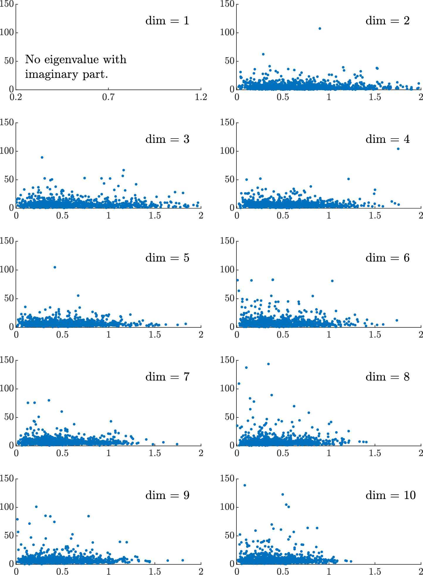
Figure 3: The scatter plot of $\min_{k}\{\left|\gamma_{i,{\bf A},k}\right|\}$ (x-axis) versus $e_{\bf K}$ (y-axis, in percentage) from dimension $1$ to $10$ for $t_{1}=1000$. The cases with $e_{\bf K}>100\%$ are not shown, but the chance of occurrence is below $1\%$.

Even though the decent performance overall, we observe that for the higher dimensional cases, LIM seems to reveal a higher $e_{\bf Q}$ whose sources are $e_{\bf A}$ and $e_{\bf K}$. This may be attributed to the eigenvalue structure of ${\bf A}$, whose eigenvalues are denoted by $\gamma_{{\bf A},k}=-\gamma_{r,{\bf A},k}+1i\cdot\gamma_{i,{\bf A},k}$ for $k=1,\dots,n$. With the abuse of notation, we drop the subscript $k$. As the dimension increases, a smaller $\gamma_{r,{\bf A}}>0$ is more likely to appear, indicating that the system has a component of slowly-decaying dynamics. Under such circumstances, it may require a longer finite realization of Eq. 2 to reveal the roles of $\gamma_{r,{\bf A}}$ in the correlation function. In the current setup $t_{1}=1000$, the existence of small $\gamma_{r,{\bf A}}$ is related to larger $e_{\bf K}$, consequently causing a larger $e_{\bf Q}$ (see Fig. 2). However, we notice that a larger $e_{\bf K}$ does not cause a serious $e_{\bf A}$, indicating that small $\gamma_{r,{\bf A}}$ may introduce an error in correlation function nearly independent of time-lag due to the lack of sampling data; namely, $K(s)=e(s){\bf K}(s)$ for some function $e(s)$ varying slowly in $s$. In $1$-dimensional case, an example $K(s)$ and ${\bf K}(s)$ shown in Fig. 1(b) reveals that the pointwise error of the numerical correlation is uniformly over time-lag, consistent with our observation. On the other hand, a smaller $\left|\gamma_{i,{\bf A}}\right|$ in the eigenvalue structure does not directly relate to a larger $e_{\bf K}$ (see Fig. 3). A possible explanation is that the random forcing mainly contributes to the radial direction rather than the spherical direction due to the symmetry of the diffusion matrix. To sum up, our numerical study implies that $\gamma_{r,{\bf A}}$ plays a major role in the relative error of covariance.

Besides, it is intriguing that the relative error $e_{\bf Q}$ strongly depends on the parity of dimension: lower in odd-dimension but higher in even-dimension. This is merely ascribed to our specific way of generating ${\bf A}$ (see Algorithm 3), resulting in a larger $\gamma_{r,{\bf A}}$ in odd dimension and hence a more accurate correlation function. Overall, to achieve a higher accuracy, a longer window of observation is required, as we see that $95$th percentiles of $e_{\bf A}$ and $e_{\bf Q}$ decrease significantly especially in higher-dimensional case as $t_{1}$ increases from $1000$ to $5000$.

Table 1: The numerical results of LIM for $t_{1}=1000$.

The Percentile of the Relative Errors of LIM: ($e_{\bf A}$i /$e_{\bf Q}$)
n	5%	12.5%	25%	50%	75%	87.5%	95%
1	[lhs][r]$0.2$/[rhs][l]$0.1$	[lhs][r]$0.5$/[rhs][l]$0.2$	[lhs][r]$1.1$/[rhs][l]$0.5$	[lhs][r]$2.3$/[rhs][l]$1.0$	[lhs][r]$4.1$/[rhs][l]$1.8$	[lhs][r]$5.5$/[rhs][l]$2.5$	[lhs][r]$7.2$/[rhs][l]$3.2$
2	[lhs][r]$0.8$/[rhs][l]$0.6$	[lhs][r]$1.3$/[rhs][l]$1.2$	[lhs][r]$2.0$/[rhs][l]$1.7$	[lhs][r]$3.9$/[rhs][l]$2.8$	[lhs][r]$6.7$/[rhs][l]$4.5$	[lhs][r]$9.5$/[rhs][l]$6.0$	[lhs][r]$14.5$/[rhs][l]$8.6$
3	[lhs][r]$2.7$/[rhs][l]$1.3$	[lhs][r]$3.9$/[rhs][l]$1.8$	[lhs][r]$5.3$/[rhs][l]$2.5$	[lhs][r]$8.6$/[rhs][l]$3.6$	[lhs][r]$12.4$/[rhs][l]$5.0$	[lhs][r]$16.7$/[rhs][l]$6.3$	[lhs][r]$23.7$/[rhs][l]$8.2$
4	[lhs][r]$1.8$/[rhs][l]$2.1$	[lhs][r]$3.0$/[rhs][l]$2.6$	[lhs][r]$4.2$/[rhs][l]$3.3$	[lhs][r]$6.5$/[rhs][l]$4.4$	[lhs][r]$9.6$/[rhs][l]$5.9$	[lhs][r]$12.8$/[rhs][l]$7.2$	[lhs][r]$17.1$/[rhs][l]$11.2$
5	[lhs][r]$3.4$/[rhs][l]$2.5$	[lhs][r]$4.7$/[rhs][l]$3.2$	[lhs][r]$6.3$/[rhs][l]$3.8$	[lhs][r]$9.0$/[rhs][l]$4.8$	[lhs][r]$12.5$/[rhs][l]$6.2$	[lhs][r]$15.9$/[rhs][l]$7.3$	[lhs][r]$20.0$/[rhs][l]$8.7$
6	[lhs][r]$2.8$/[rhs][l]$3.3$	[lhs][r]$3.7$/[rhs][l]$3.9$	[lhs][r]$5.2$/[rhs][l]$4.6$	[lhs][r]$7.5$/[rhs][l]$5.8$	[lhs][r]$10.2$/[rhs][l]$7.3$	[lhs][r]$13.0$/[rhs][l]$9.4$	[lhs][r]$16.1$/[rhs][l]$20.1$
7	[lhs][r]$3.8$/[rhs][l]$3.6$	[lhs][r]$5.0$/[rhs][l]$4.4$	[lhs][r]$6.7$/[rhs][l]$5.0$	[lhs][r]$9.1$/[rhs][l]$6.1$	[lhs][r]$12.3$/[rhs][l]$7.4$	[lhs][r]$15.1$/[rhs][l]$9.0$	[lhs][r]$18.2$/[rhs][l]$14.1$
8	[lhs][r]$3.5$/[rhs][l]$4.4$	[lhs][r]$4.7$/[rhs][l]$5.2$	[lhs][r]$6.2$/[rhs][l]$5.9$	[lhs][r]$8.6$/[rhs][l]$7.3$	[lhs][r]$11.4$/[rhs][l]$9.6$	[lhs][r]$13.8$/[rhs][l]$13.5$	[lhs][r]$17.1$/[rhs][l]$27.1$
9	[lhs][r]$4.4$/[rhs][l]$4.9$	[lhs][r]$5.6$/[rhs][l]$5.6$	[lhs][r]$7.3$/[rhs][l]$6.3$	[lhs][r]$9.8$/[rhs][l]$7.7$	[lhs][r]$12.7$/[rhs][l]$9.5$	[lhs][r]$15.4$/[rhs][l]$12.3$	[lhs][r]$18.8$/[rhs][l]$22.6$
10	[lhs][r]$4.3$/[rhs][l]$5.7$	[lhs][r]$5.6$/[rhs][l]$6.5$	[lhs][r]$7.0$/[rhs][l]$7.3$	[lhs][r]$9.5$/[rhs][l]$8.8$	[lhs][r]$12.2$/[rhs][l]$11.3$	[lhs][r]$14.6$/[rhs][l]$15.8$	[lhs][r]$16.9$/[rhs][l]$35.5$

• The percentile of the relative errors $e_{\bf A}$/$e_{\bf Q}$ in percentage out of $1024$ trials.

• The time-lag applied in Algorithm 1 is set to be $\rho=0.5$.

Table 2: The numerical results of LIM for $t_{1}=5000$.

The Percentile of the Relative Errors of LIM: ($e_{\bf A}$/$e_{\bf Q}$)
n	5%	12.5%	25%	50%	75%	87.5%	95%
1	[lhs][r]$0.2$/[rhs][l]$0.1$	[lhs][r]$0.5$/[rhs][l]$0.2$	[lhs][r]$1.1$/[rhs][l]$0.5$	[lhs][r]$2.3$/[rhs][l]$1.1$	[lhs][r]$4.0$/[rhs][l]$1.9$	[lhs][r]$5.4$/[rhs][l]$2.5$	[lhs][r]$6.9$/[rhs][l]$3.0$
2	[lhs][r]$0.3$/[rhs][l]$0.3$	[lhs][r]$0.5$/[rhs][l]$0.5$	[lhs][r]$0.9$/[rhs][l]$0.8$	[lhs][r]$1.7$/[rhs][l]$1.3$	[lhs][r]$3.0$/[rhs][l]$2.0$	[lhs][r]$4.6$/[rhs][l]$2.5$	[lhs][r]$6.4$/[rhs][l]$3.3$
3	[lhs][r]$1.2$/[rhs][l]$0.6$	[lhs][r]$1.8$/[rhs][l]$0.8$	[lhs][r]$2.5$/[rhs][l]$1.1$	[lhs][r]$3.7$/[rhs][l]$1.6$	[lhs][r]$5.5$/[rhs][l]$2.2$	[lhs][r]$7.1$/[rhs][l]$2.8$	[lhs][r]$10.3$/[rhs][l]$3.4$
4	[lhs][r]$0.8$/[rhs][l]$0.9$	[lhs][r]$1.2$/[rhs][l]$1.2$	[lhs][r]$1.8$/[rhs][l]$1.4$	[lhs][r]$2.8$/[rhs][l]$1.9$	[lhs][r]$4.1$/[rhs][l]$2.5$	[lhs][r]$5.5$/[rhs][l]$3.0$	[lhs][r]$7.6$/[rhs][l]$3.9$
5	[lhs][r]$1.5$/[rhs][l]$1.2$	[lhs][r]$2.1$/[rhs][l]$1.4$	[lhs][r]$2.9$/[rhs][l]$1.7$	[lhs][r]$4.0$/[rhs][l]$2.2$	[lhs][r]$5.6$/[rhs][l]$2.7$	[lhs][r]$7.0$/[rhs][l]$3.3$	[lhs][r]$9.0$/[rhs][l]$3.9$
6	[lhs][r]$1.2$/[rhs][l]$1.4$	[lhs][r]$1.7$/[rhs][l]$1.7$	[lhs][r]$2.4$/[rhs][l]$2.0$	[lhs][r]$3.4$/[rhs][l]$2.5$	[lhs][r]$4.5$/[rhs][l]$3.2$	[lhs][r]$5.7$/[rhs][l]$3.9$	[lhs][r]$7.3$/[rhs][l]$6.1$
7	[lhs][r]$1.8$/[rhs][l]$1.7$	[lhs][r]$2.3$/[rhs][l]$1.9$	[lhs][r]$3.1$/[rhs][l]$2.1$	[lhs][r]$4.3$/[rhs][l]$2.7$	[lhs][r]$5.5$/[rhs][l]$3.3$	[lhs][r]$6.8$/[rhs][l]$3.9$	[lhs][r]$8.9$/[rhs][l]$5.1$
8	[lhs][r]$1.6$/[rhs][l]$2.0$	[lhs][r]$2.2$/[rhs][l]$2.3$	[lhs][r]$2.7$/[rhs][l]$2.6$	[lhs][r]$3.8$/[rhs][l]$3.2$	[lhs][r]$5.1$/[rhs][l]$3.9$	[lhs][r]$6.1$/[rhs][l]$5.0$	[lhs][r]$7.5$/[rhs][l]$7.9$
9	[lhs][r]$1.7$/[rhs][l]$2.2$	[lhs][r]$2.5$/[rhs][l]$2.5$	[lhs][r]$3.2$/[rhs][l]$2.8$	[lhs][r]$4.4$/[rhs][l]$3.4$	[lhs][r]$5.7$/[rhs][l]$4.1$	[lhs][r]$6.7$/[rhs][l]$5.0$	[lhs][r]$8.1$/[rhs][l]$7.8$
10	[lhs][r]$1.9$/[rhs][l]$2.5$	[lhs][r]$2.5$/[rhs][l]$2.8$	[lhs][r]$3.1$/[rhs][l]$3.1$	[lhs][r]$4.2$/[rhs][l]$3.8$	[lhs][r]$5.4$/[rhs][l]$4.9$	[lhs][r]$6.5$/[rhs][l]$6.9$	[lhs][r]$7.8$/[rhs][l]$13.5$

• See the table note in Table 1.

4.2 The performance of Colored-LIM

The performance of Colored-LIM over $1024$ trials for different dimensions and parameters are presented in Tables 3, 4, and 5. The numerical derivatives are computed by central finite difference methods. Though the accuracy of Colored-LIM depends on the noise correlation time $\tau$ and the observation time-span, Colored-LIM reaches an acceptable accuracy provided that a sufficiently long observation time-span, with median values of $e_{\bf A}$ and $e_{\bf Q}$ ranging from $1.2\%$ to $6.4\%$, comparable with those of LIM.

The dependence of $e_{\bf A}$ on $\tau$ arises from the accuracy of the approximation Eq. 8. For a smaller $\tau$, the colored-noise process and hence the stochastic process oscillates faster compared to the larger $\tau$ case. Therefore, a relatively smaller window of observation is sufficient to obtain a reliable result since loosely speaking, the pair $\big{(}x(\cdot),x(\cdot+s)\big{)}$ of observation and its delay is more likely to run over all possibilities within a shorter time. On the other hand, in the large $\tau$ case, the time correlation of noises slows down the oscillation of the stochastic process, so it takes a longer time for $\big{(}x(\cdot),x(\cdot+s)\big{)}$ to walk through its state space, similar to the effect of slowly-decaying dynamics. In addition, when the observation is sufficiently long, the numerical computation of the correlation function and its derivatives is accurate enough, with median values ranging from $0.8\%$ to $9.2\%$, and does not suffer from the noise amplification effect, as shown in Table 6. In our study, to achieve higher accuracy in $e_{\bf A}$, a time-span $t_{1}=5000$ is required for $\tau=0.5$ while a shorter window of observation $t_{1}=1000$ is sufficient for $\tau=0.1$, as shown in Tables 3 and 5.

In the classical LIM case, the diffusion matrix ${Q_{\text{LIM}}}$ is directly computed via ${A_{\text{LIM}}}$ and $K(0)$, meaning that roughly speaking, $e_{\bf Q}$ is proportional to $e_{\bf A}$ and $e_{\bf K}$. However, in Colored-LIM, ${Q_{\text{C-LIM}}}$ is the solution of Eq. 13 or Eq. 17. Therefore, the inaccuracy of ${Q_{\text{C-LIM}}}$ comes from not only that of ${A_{\text{C-LIM}}}$ and $K(0)$ as discussed before, but also from the potential ill-posedness of the linear system that solves ${Q_{\text{C-LIM}}}$, which can be measured by the condition number. To investigate the potential sources, Tables 3, 4, and 5 also summarize (a) the number of cases where $e_{\bf K}\geq 15\%$, where the condition number of the linear equation that solves ${Q_{\text{C-LIM}}}$ is larger than $20$, and where those values are within tolerance, and (b) under such conditions, the number of cases where $e_{\bf Q}\geq 15\%$. We see in Table 5 that a higher $e_{\bf K}$ inevitably leads to a higher $e_{\bf Q}$ and the ill-posedness based on either Eq. 13 or Eq. 17 has a decent chance to amplify $e_{\bf Q}$. Nevertheless, for higher dimensional cases, the number of trials with large condition numbers based on Eq. 17 is less than the number of those based on Eq. 13 due to the dimensional issue. Simply speaking, Eq. 17 is a $n$-dimensional problem while Eq. 13 is higher-dimensional. For instance, if Eq. 13 is transformed into a linear equation of the form $Mx=b$, then $M$ can be a $\frac{n(n+1)}{2}$-dimensional square matrix which is more likely to have smaller eigenvalues in magnitude in our setup, or even in practice if a multi-scale dynamics is considered. On the other hand, for smaller dimensional cases, as the conditional numbers are in general moderate, the use of Eq. 17 introduces an additional error $e_{{\bf K}^{\prime}}$, which may further cause a higher $e_{\bf Q}$.

Although the performance in ${Q_{\text{C-LIM}}}$ based on Eq. 13 or Eq. 17 is the result of the competing effect of condition number and $e_{{\bf K}^{\prime}}$, we remark that in general, $K^{\prime}(0)$ can be improved by taking a longer period of observation as shown in Table 6, while the condition number is the nature of $\tau$, ${\bf A}$ and ${\bf Q}$ of the underlying linear SDE. In our setup, larger $\tau$ and higher dimensionality tend to increase the chance of ill-posedness due to large eigenvalues in magnitude in ${B_{\text{C-LIM}}}$, suggesting that Eq. 17 is suitable for $\tau=0.5$ and $n\geq 7$. Moreover, as before, since the error in correlation function may be introduced uniformly near the origin, the relative errors $e_{{\bf K}^{(m)}}$ for $m=0,\dots,3$ may partially cancel out in the computation of ${A_{\text{C-LIM}}}$, leading to a moderate $e_{\bf A}$. Nevertheless, overall, Colored-LIM achieves a decent accuracy provided that sufficient sampling is given.

Table 3: The numerical results for $\tau=0.1$ and $t_{1}=1000$.

The Percentile of the Relative Errors of Colored-LIM: ($e_{\bf A}$/$e_{\bf Q}$i )
n	5%	12.5%	25%	50%	75%	87.5%	95%
1	[lhs][r]$0.3$/[rhs][l]$0.1$	[lhs][r]$0.9$/[rhs][l]$0.3$	[lhs][r]$1.9$/[rhs][l]$0.6$	[lhs][r]$3.9$/[rhs][l]$1.2$	[lhs][r]$6.8$/[rhs][l]$2.0$	[lhs][r]$9.4$/[rhs][l]$2.5$	[lhs][r]$12.5$/[rhs][l]$3.1$
2	[lhs][r]$0.7$/[rhs][l]$0.3$	[lhs][r]$1.1$/[rhs][l]$0.5$	[lhs][r]$1.7$/[rhs][l]$0.8$	[lhs][r]$3.1$/[rhs][l]$1.4$	[lhs][r]$5.2$/[rhs][l]$2.1$	[lhs][r]$7.1$/[rhs][l]$2.7$	[lhs][r]$10.6$/[rhs][l]$3.3$
3	[lhs][r]$2.0$/[rhs][l]$0.6$	[lhs][r]$3.0$/[rhs][l]$0.9$	[lhs][r]$4.3$/[rhs][l]$1.2$	[lhs][r]$6.4$/[rhs][l]$1.7$	[lhs][r]$9.6$/[rhs][l]$2.3$	[lhs][r]$12.8$/[rhs][l]$2.8$	[lhs][r]$17.8$/[rhs][l]$3.3$
4	[lhs][r]$1.5$/[rhs][l]$0.9$	[lhs][r]$2.3$/[rhs][l]$1.1$	[lhs][r]$3.3$/[rhs][l]$1.5$	[lhs][r]$5.0$/[rhs][l]$2.0$	[lhs][r]$6.9$/[rhs][l]$2.5$	[lhs][r]$8.8$/[rhs][l]$3.0$	[lhs][r]$11.8$/[rhs][l]$4.0$
5	[lhs][r]$2.5$/[rhs][l]$1.1$	[lhs][r]$3.5$/[rhs][l]$1.4$	[lhs][r]$4.6$/[rhs][l]$1.6$	[lhs][r]$6.4$/[rhs][l]$2.1$	[lhs][r]$9.0$/[rhs][l]$2.6$	[lhs][r]$11.4$/[rhs][l]$3.1$	[lhs][r]$14.8$/[rhs][l]$3.8$
6	[lhs][r]$1.9$/[rhs][l]$1.3$	[lhs][r]$3.0$/[rhs][l]$1.6$	[lhs][r]$3.9$/[rhs][l]$1.9$	[lhs][r]$5.4$/[rhs][l]$2.3$	[lhs][r]$7.3$/[rhs][l]$2.9$	[lhs][r]$8.8$/[rhs][l]$3.3$	[lhs][r]$10.8$/[rhs][l]$5.1$
7	[lhs][r]$3.0$/[rhs][l]$1.5$	[lhs][r]$3.8$/[rhs][l]$1.7$	[lhs][r]$4.8$/[rhs][l]$1.9$	[lhs][r]$6.4$/[rhs][l]$2.4$	[lhs][r]$8.3$/[rhs][l]$2.9$	[lhs][r]$10.0$/[rhs][l]$3.3$	[lhs][r]$12.3$/[rhs][l]$4.3$
8	[lhs][r]$2.2$/[rhs][l]$1.7$	[lhs][r]$3.2$/[rhs][l]$2.0$	[lhs][r]$4.2$/[rhs][l]$2.2$	[lhs][r]$5.6$/[rhs][l]$2.6$	[lhs][r]$7.4$/[rhs][l]$3.2$	[lhs][r]$8.9$/[rhs][l]$3.9$	[lhs][r]$10.7$/[rhs][l]$7.0$
9	[lhs][r]$2.7$/[rhs][l]$1.8$	[lhs][r]$3.6$/[rhs][l]$2.1$	[lhs][r]$4.7$/[rhs][l]$2.3$	[lhs][r]$6.3$/[rhs][l]$2.8$	[lhs][r]$8.0$/[rhs][l]$3.2$	[lhs][r]$9.7$/[rhs][l]$3.8$	[lhs][r]$11.6$/[rhs][l]$5.9$
10	[lhs][r]$2.4$/[rhs][l]$2.0$	[lhs][r]$3.4$/[rhs][l]$2.2$	[lhs][r]$4.2$/[rhs][l]$2.5$	[lhs][r]$5.6$/[rhs][l]$3.0$	[lhs][r]$7.2$/[rhs][l]$3.6$	[lhs][r]$8.6$/[rhs][l]$5.2$	[lhs][r]$10.4$/[rhs][l]$11.4$

• In percentage, out of $1024$ trials.

The Analysis of $e_{\bf Q}$ⁱ n ${\bf C}_{\bf Q}$ⁱⁱ ${\bf C}_{\bf K}$ⁱⁱⁱ ${\bf C}_{\textbf{cond.}}$ⁱⁱⁱ Cⁱⁱⁱ n ${\bf C}_{\bf Q}$ ${\bf C}_{\bf K}$ ${\bf C}_{\textbf{cond.}}$ C 1 0 [lhs][r]$0$/[rhs][l]$30$ [lhs][r]$0$/[rhs][l]$0$ [lhs][r]$0$/[rhs][l]$994$ 6 18 [lhs][r]$13$/[rhs][l]$91$ [lhs][r]$6$/[rhs][l]$10$ [lhs][r]$3$/[rhs][l]$927$ 2 1 [lhs][r]$1$/[rhs][l]$59$ [lhs][r]$0$/[rhs][l]$0$ [lhs][r]$0$/[rhs][l]$965$ 7 7 [lhs][r]$3$/[rhs][l]$75$ [lhs][r]$4$/[rhs][l]$7$ [lhs][r]$2$/[rhs][l]$945$ 3 0 [lhs][r]$0$/[rhs][l]$93$ [lhs][r]$0$/[rhs][l]$0$ [lhs][r]$0$/[rhs][l]$931$ 8 25 [lhs][r]$15$/[rhs][l]$98$ [lhs][r]$9$/[rhs][l]$16$ [lhs][r]$7$/[rhs][l]$917$ 4 12 [lhs][r]$9$/[rhs][l]$69$ [lhs][r]$2$/[rhs][l]$2$ [lhs][r]$3$/[rhs][l]$955$ 9 18 [lhs][r]$14$/[rhs][l]$72$ [lhs][r]$11$/[rhs][l]$20$ [lhs][r]$1$/[rhs][l]$942$ 5 6 [lhs][r]$6$/[rhs][l]$78$ [lhs][r]$0$/[rhs][l]$3$ [lhs][r]$0$/[rhs][l]$943$ 10 38 [lhs][r]$27$/[rhs][l]$99$ [lhs][r]$20$/[rhs][l]$34$ [lhs][r]$4$/[rhs][l]$907$ i $e_{\bf Q}$ is computed based on Eq. (13).

The Percentile of the Relative Errors of Colored-LIM: ($e_{\bf A}$/$e_{\bf Q}$iv  )
n	5%	12.5%	25%	50%	75%	87.5%	95%
1	[lhs][r]$0.3$/[rhs][l]$0.1$	[lhs][r]$0.9$/[rhs][l]$0.3$	[lhs][r]$1.9$/[rhs][l]$0.7$	[lhs][r]$3.9$/[rhs][l]$1.4$	[lhs][r]$6.8$/[rhs][l]$2.3$	[lhs][r]$9.4$/[rhs][l]$2.8$	[lhs][r]$12.5$/[rhs][l]$3.5$
2	[lhs][r]$0.7$/[rhs][l]$0.6$	[lhs][r]$1.1$/[rhs][l]$0.9$	[lhs][r]$1.7$/[rhs][l]$1.4$	[lhs][r]$3.1$/[rhs][l]$2.1$	[lhs][r]$5.2$/[rhs][l]$2.9$	[lhs][r]$7.1$/[rhs][l]$3.8$	[lhs][r]$10.6$/[rhs][l]$5.4$
3	[lhs][r]$2.0$/[rhs][l]$1.0$	[lhs][r]$3.0$/[rhs][l]$1.3$	[lhs][r]$4.3$/[rhs][l]$1.7$	[lhs][r]$6.4$/[rhs][l]$2.3$	[lhs][r]$9.6$/[rhs][l]$3.0$	[lhs][r]$12.8$/[rhs][l]$3.8$	[lhs][r]$17.8$/[rhs][l]$6.6$
4	[lhs][r]$1.5$/[rhs][l]$1.5$	[lhs][r]$2.3$/[rhs][l]$1.8$	[lhs][r]$3.3$/[rhs][l]$2.2$	[lhs][r]$5.0$/[rhs][l]$2.7$	[lhs][r]$6.9$/[rhs][l]$3.6$	[lhs][r]$8.8$/[rhs][l]$4.7$	[lhs][r]$11.8$/[rhs][l]$10.4$
5	[lhs][r]$2.5$/[rhs][l]$1.7$	[lhs][r]$3.5$/[rhs][l]$2.0$	[lhs][r]$4.6$/[rhs][l]$2.3$	[lhs][r]$6.4$/[rhs][l]$2.8$	[lhs][r]$9.0$/[rhs][l]$3.6$	[lhs][r]$11.4$/[rhs][l]$4.5$	[lhs][r]$14.8$/[rhs][l]$7.3$
6	[lhs][r]$1.9$/[rhs][l]$2.0$	[lhs][r]$3.0$/[rhs][l]$2.4$	[lhs][r]$3.9$/[rhs][l]$2.8$	[lhs][r]$5.4$/[rhs][l]$3.4$	[lhs][r]$7.3$/[rhs][l]$4.3$	[lhs][r]$8.8$/[rhs][l]$6.9$	[lhs][r]$10.8$/[rhs][l]$15.9$
7	[lhs][r]$3.0$/[rhs][l]$2.1$	[lhs][r]$3.8$/[rhs][l]$2.4$	[lhs][r]$4.8$/[rhs][l]$2.8$	[lhs][r]$6.4$/[rhs][l]$3.4$	[lhs][r]$8.3$/[rhs][l]$4.1$	[lhs][r]$10.0$/[rhs][l]$5.4$	[lhs][r]$12.3$/[rhs][l]$10.0$
8	[lhs][r]$2.2$/[rhs][l]$2.5$	[lhs][r]$3.2$/[rhs][l]$2.9$	[lhs][r]$4.2$/[rhs][l]$3.3$	[lhs][r]$5.6$/[rhs][l]$3.9$	[lhs][r]$7.4$/[rhs][l]$5.4$	[lhs][r]$8.9$/[rhs][l]$8.5$	[lhs][r]$10.7$/[rhs][l]$21.9$
9	[lhs][r]$2.7$/[rhs][l]$2.6$	[lhs][r]$3.6$/[rhs][l]$3.0$	[lhs][r]$4.7$/[rhs][l]$3.3$	[lhs][r]$6.3$/[rhs][l]$3.9$	[lhs][r]$8.0$/[rhs][l]$4.9$	[lhs][r]$9.7$/[rhs][l]$7.2$	[lhs][r]$11.6$/[rhs][l]$16.0$
10	[lhs][r]$2.4$/[rhs][l]$3.0$	[lhs][r]$3.4$/[rhs][l]$3.3$	[lhs][r]$4.2$/[rhs][l]$3.7$	[lhs][r]$5.6$/[rhs][l]$4.5$	[lhs][r]$7.2$/[rhs][l]$6.5$	[lhs][r]$8.6$/[rhs][l]$10.1$	[lhs][r]$10.4$/[rhs][l]$26.3$

• In percentage, out of $1024$ trials.

The Analysis of $e_{\bf Q}$^iv n ${\bf C}_{\bf Q}$ ${\bf C}_{{\bf K},{\bf K}^{\prime}}$ⁱⁱⁱ ${\bf C}_{\textbf{cond.}}$ C n ${\bf C}_{\bf Q}$ ${\bf C}_{{\bf K},{\bf K}^{\prime}}$ ${\bf C}_{\textbf{cond.}}$ C 1 0 [lhs][r]$0$/[rhs][l]$30$ [lhs][r]$0$/[rhs][l]$0$ [lhs][r]$0$/[rhs][l]$994$ 6 53 [lhs][r]$33$/[rhs][l]$103$ [lhs][r]$4$/[rhs][l]$5$ [lhs][r]$20$/[rhs][l]$921$ 2 16 [lhs][r]$12$/[rhs][l]$86$ [lhs][r]$0$/[rhs][l]$0$ [lhs][r]$4$/[rhs][l]$938$ 7 35 [lhs][r]$20$/[rhs][l]$91$ [lhs][r]$2$/[rhs][l]$2$ [lhs][r]$15$/[rhs][l]$933$ 3 23 [lhs][r]$16$/[rhs][l]$187$ [lhs][r]$0$/[rhs][l]$0$ [lhs][r]$7$/[rhs][l]$837$ 8 73 [lhs][r]$38$/[rhs][l]$109$ [lhs][r]$8$/[rhs][l]$8$ [lhs][r]$32$/[rhs][l]$912$ 4 42 [lhs][r]$22$/[rhs][l]$87$ [lhs][r]$2$/[rhs][l]$2$ [lhs][r]$20$/[rhs][l]$937$ 9 54 [lhs][r]$30$/[rhs][l]$93$ [lhs][r]$8$/[rhs][l]$11$ [lhs][r]$23$/[rhs][l]$929$ 5 29 [lhs][r]$21$/[rhs][l]$101$ [lhs][r]$1$/[rhs][l]$1$ [lhs][r]$8$/[rhs][l]$923$ 10 89 [lhs][r]$51$/[rhs][l]$115$ [lhs][r]$16$/[rhs][l]$24$ [lhs][r]$35$/[rhs][l]$901$ iv $e_{\bf Q}$ is computed based on Eq. (17). ii, iii ${\bf C}_{\bf Q}$, ${\bf C}_{\bf K}$, ${\bf C}_{{\bf K},{\bf K}^{\prime}}$,${\bf C}_{\textbf{cond.}}$ and ${\bf C}$ indicate conditions where the trials with $e_{\bf Q}>15\%$, the trials with $e_{\bf K}>15\%$, the trials with $e_{\bf K}>15\%$ or $e_{\bf K}^{\prime}>15\%$, the trials with condition number $>20$, and trials not satisfying ${\bf C}_{\bf K}$ (or ${\bf C}_{\bf K}^{\prime}$) and ${\bf C}_{\textbf{cond.}}$, respectively. ii The column shows the number of trials satisfying ${\bf C}_{\bf Q}$. iii $*/**$ shows the conditional probability that $e_{\bf Q}>15\%$ when the condition ${\bf C}_{\bullet}$ is satisfied.

Table 4: The numerical results for $\tau=0.1$ and $t_{1}=5000$.

The Percentile of the Relative Errors of Colored-LIM: ($e_{\bf A}$/$e_{\bf Q}$i )
n	5%	12.5%	25%	50%	75%	87.5%	95%
1	[lhs][r]$0.2$/[rhs][l]$0.1$	[lhs][r]$0.4$/[rhs][l]$0.3$	[lhs][r]$0.8$/[rhs][l]$0.5$	[lhs][r]$1.9$/[rhs][l]$0.9$	[lhs][r]$3.2$/[rhs][l]$1.3$	[lhs][r]$4.2$/[rhs][l]$1.6$	[lhs][r]$5.5$/[rhs][l]$1.9$
2	[lhs][r]$0.3$/[rhs][l]$0.2$	[lhs][r]$0.5$/[rhs][l]$0.4$	[lhs][r]$0.8$/[rhs][l]$0.5$	[lhs][r]$1.4$/[rhs][l]$0.9$	[lhs][r]$2.4$/[rhs][l]$1.3$	[lhs][r]$3.2$/[rhs][l]$1.5$	[lhs][r]$4.9$/[rhs][l]$1.9$
3	[lhs][r]$1.0$/[rhs][l]$0.4$	[lhs][r]$1.5$/[rhs][l]$0.5$	[lhs][r]$2.0$/[rhs][l]$0.7$	[lhs][r]$2.9$/[rhs][l]$1.0$	[lhs][r]$4.3$/[rhs][l]$1.4$	[lhs][r]$5.5$/[rhs][l]$1.6$	[lhs][r]$7.4$/[rhs][l]$1.9$
4	[lhs][r]$0.7$/[rhs][l]$0.5$	[lhs][r]$1.1$/[rhs][l]$0.7$	[lhs][r]$1.5$/[rhs][l]$0.8$	[lhs][r]$2.2$/[rhs][l]$1.1$	[lhs][r]$3.1$/[rhs][l]$1.4$	[lhs][r]$3.9$/[rhs][l]$1.6$	[lhs][r]$4.9$/[rhs][l]$2.0$
5	[lhs][r]$1.2$/[rhs][l]$0.6$	[lhs][r]$1.6$/[rhs][l]$0.7$	[lhs][r]$2.1$/[rhs][l]$0.9$	[lhs][r]$2.9$/[rhs][l]$1.1$	[lhs][r]$3.9$/[rhs][l]$1.4$	[lhs][r]$4.9$/[rhs][l]$1.7$	[lhs][r]$6.1$/[rhs][l]$2.0$
6	[lhs][r]$1.0$/[rhs][l]$0.7$	[lhs][r]$1.3$/[rhs][l]$0.9$	[lhs][r]$1.7$/[rhs][l]$1.0$	[lhs][r]$2.4$/[rhs][l]$1.3$	[lhs][r]$3.2$/[rhs][l]$1.6$	[lhs][r]$3.9$/[rhs][l]$1.9$	[lhs][r]$4.7$/[rhs][l]$2.7$
7	[lhs][r]$1.3$/[rhs][l]$0.8$	[lhs][r]$1.7$/[rhs][l]$0.9$	[lhs][r]$2.1$/[rhs][l]$1.1$	[lhs][r]$2.8$/[rhs][l]$1.3$	[lhs][r]$3.8$/[rhs][l]$1.5$	[lhs][r]$4.5$/[rhs][l]$1.8$	[lhs][r]$5.7$/[rhs][l]$2.3$
8	[lhs][r]$1.1$/[rhs][l]$0.9$	[lhs][r]$1.5$/[rhs][l]$1.0$	[lhs][r]$1.9$/[rhs][l]$1.2$	[lhs][r]$2.5$/[rhs][l]$1.4$	[lhs][r]$3.2$/[rhs][l]$1.7$	[lhs][r]$3.8$/[rhs][l]$2.2$	[lhs][r]$4.7$/[rhs][l]$4.6$
9	[lhs][r]$1.4$/[rhs][l]$1.0$	[lhs][r]$1.7$/[rhs][l]$1.1$	[lhs][r]$2.1$/[rhs][l]$1.2$	[lhs][r]$2.7$/[rhs][l]$1.4$	[lhs][r]$3.6$/[rhs][l]$1.7$	[lhs][r]$4.2$/[rhs][l]$2.1$	[lhs][r]$5.0$/[rhs][l]$3.8$
10	[lhs][r]$1.2$/[rhs][l]$1.1$	[lhs][r]$1.6$/[rhs][l]$1.2$	[lhs][r]$1.9$/[rhs][l]$1.3$	[lhs][r]$2.5$/[rhs][l]$1.6$	[lhs][r]$3.2$/[rhs][l]$2.0$	[lhs][r]$3.7$/[rhs][l]$3.2$	[lhs][r]$4.5$/[rhs][l]$7.2$

• Unit in percentage, out of $1024$ trials.

The Analysis of $e_{\bf Q}$ⁱ n ${\bf C}_{\bf Q}$ ${\bf C}_{\bf K}$ ${\bf C}_{\textbf{cond.}}$ C n ${\bf C}_{\bf Q}$ ${\bf C}_{\bf K}$ ${\bf C}_{\textbf{cond.}}$ C 1 0 [lhs][r]$0$/[rhs][l]$0$ [lhs][r]$0$/[rhs][l]$0$ [lhs][r]$0$/[rhs][l]$1024$ 6 10 [lhs][r]$9$/[rhs][l]$37$ [lhs][r]$8$/[rhs][l]$9$ [lhs][r]$0$/[rhs][l]$986$ 2 0 [lhs][r]$0$/[rhs][l]$14$ [lhs][r]$0$/[rhs][l]$0$ [lhs][r]$0$/[rhs][l]$1010$ 7 7 [lhs][r]$6$/[rhs][l]$22$ [lhs][r]$6$/[rhs][l]$9$ [lhs][r]$0$/[rhs][l]$998$ 3 0 [lhs][r]$0$/[rhs][l]$9$ [lhs][r]$0$/[rhs][l]$0$ [lhs][r]$0$/[rhs][l]$1015$ 8 18 [lhs][r]$13$/[rhs][l]$54$ [lhs][r]$14$/[rhs][l]$22$ [lhs][r]$1$/[rhs][l]$960$ 4 4 [lhs][r]$4$/[rhs][l]$20$ [lhs][r]$2$/[rhs][l]$4$ [lhs][r]$0$/[rhs][l]$1004$ 9 11 [lhs][r]$7$/[rhs][l]$33$ [lhs][r]$9$/[rhs][l]$16$ [lhs][r]$0$/[rhs][l]$982$ 5 3 [lhs][r]$2$/[rhs][l]$23$ [lhs][r]$1$/[rhs][l]$1$ [lhs][r]$0$/[rhs][l]$1000$ 10 29 [lhs][r]$14$/[rhs][l]$46$ [lhs][r]$24$/[rhs][l]$34$ [lhs][r]$1$/[rhs][l]$955$ i $e_{\bf Q}$ is computed based on Eq. (13).

The Percentile of the Relative Errors of Colored-LIM: ($e_{\bf A}$/$e_{\bf Q}$ii  )
n	5%	12.5%	25%	50%	75%	87.5%	95%
1	[lhs][r]$0.2$/[rhs][l]$0.3$	[lhs][r]$0.4$/[rhs][l]$0.5$	[lhs][r]$0.8$/[rhs][l]$0.8$	[lhs][r]$1.9$/[rhs][l]$1.2$	[lhs][r]$3.2$/[rhs][l]$1.7$	[lhs][r]$4.2$/[rhs][l]$2.0$	[lhs][r]$5.5$/[rhs][l]$2.3$
2	[lhs][r]$0.3$/[rhs][l]$0.5$	[lhs][r]$0.5$/[rhs][l]$0.7$	[lhs][r]$0.8$/[rhs][l]$1.0$	[lhs][r]$1.4$/[rhs][l]$1.4$	[lhs][r]$2.4$/[rhs][l]$1.8$	[lhs][r]$3.2$/[rhs][l]$2.1$	[lhs][r]$4.9$/[rhs][l]$2.5$
3	[lhs][r]$1.0$/[rhs][l]$0.7$	[lhs][r]$1.5$/[rhs][l]$0.9$	[lhs][r]$2.0$/[rhs][l]$1.1$	[lhs][r]$2.9$/[rhs][l]$1.5$	[lhs][r]$4.3$/[rhs][l]$1.8$	[lhs][r]$5.5$/[rhs][l]$2.1$	[lhs][r]$7.4$/[rhs][l]$2.4$
4	[lhs][r]$0.7$/[rhs][l]$1.0$	[lhs][r]$1.1$/[rhs][l]$1.1$	[lhs][r]$1.5$/[rhs][l]$1.3$	[lhs][r]$2.2$/[rhs][l]$1.6$	[lhs][r]$3.1$/[rhs][l]$2.0$	[lhs][r]$3.9$/[rhs][l]$2.4$	[lhs][r]$4.9$/[rhs][l]$3.6$
5	[lhs][r]$1.2$/[rhs][l]$1.1$	[lhs][r]$1.6$/[rhs][l]$1.2$	[lhs][r]$2.1$/[rhs][l]$1.4$	[lhs][r]$2.9$/[rhs][l]$1.7$	[lhs][r]$3.9$/[rhs][l]$2.0$	[lhs][r]$4.9$/[rhs][l]$2.4$	[lhs][r]$6.1$/[rhs][l]$2.9$
6	[lhs][r]$1.0$/[rhs][l]$1.3$	[lhs][r]$1.3$/[rhs][l]$1.5$	[lhs][r]$1.7$/[rhs][l]$1.7$	[lhs][r]$2.4$/[rhs][l]$2.0$	[lhs][r]$3.2$/[rhs][l]$2.3$	[lhs][r]$3.9$/[rhs][l]$2.9$	[lhs][r]$4.7$/[rhs][l]$4.8$
7	[lhs][r]$1.3$/[rhs][l]$1.3$	[lhs][r]$1.7$/[rhs][l]$1.5$	[lhs][r]$2.1$/[rhs][l]$1.7$	[lhs][r]$2.8$/[rhs][l]$2.0$	[lhs][r]$3.8$/[rhs][l]$2.3$	[lhs][r]$4.5$/[rhs][l]$2.6$	[lhs][r]$5.7$/[rhs][l]$3.8$
8	[lhs][r]$1.1$/[rhs][l]$1.5$	[lhs][r]$1.5$/[rhs][l]$1.7$	[lhs][r]$1.9$/[rhs][l]$1.9$	[lhs][r]$2.5$/[rhs][l]$2.2$	[lhs][r]$3.2$/[rhs][l]$2.6$	[lhs][r]$3.8$/[rhs][l]$3.5$	[lhs][r]$4.7$/[rhs][l]$6.4$
9	[lhs][r]$1.4$/[rhs][l]$1.6$	[lhs][r]$1.7$/[rhs][l]$1.7$	[lhs][r]$2.1$/[rhs][l]$1.9$	[lhs][r]$2.7$/[rhs][l]$2.1$	[lhs][r]$3.6$/[rhs][l]$2.5$	[lhs][r]$4.2$/[rhs][l]$3.0$	[lhs][r]$5.0$/[rhs][l]$4.2$
10	[lhs][r]$1.2$/[rhs][l]$1.7$	[lhs][r]$1.6$/[rhs][l]$1.9$	[lhs][r]$1.9$/[rhs][l]$2.1$	[lhs][r]$2.5$/[rhs][l]$2.4$	[lhs][r]$3.2$/[rhs][l]$3.0$	[lhs][r]$3.7$/[rhs][l]$3.9$	[lhs][r]$4.5$/[rhs][l]$7.8$

• Unit in percentage, out of $1024$ trials.

The Analysis of $e_{\bf Q}$ⁱⁱ n ${\bf C}_{\bf Q}$ ${\bf C}_{{\bf K},{\bf K}^{\prime}}$ ${\bf C}_{\textbf{cond.}}$ C n ${\bf C}_{\bf Q}$ ${\bf C}_{{\bf K},{\bf K}^{\prime}}$ ${\bf C}_{\textbf{cond.}}$ C 1 0 [lhs][r]$0$/[rhs][l]$0$ [lhs][r]$0$/[rhs][l]$0$ [lhs][r]$0$/[rhs][l]$1024$ 6 16 [lhs][r]$15$/[rhs][l]$39$ [lhs][r]$6$/[rhs][l]$6$ [lhs][r]$1$/[rhs][l]$985$ 2 8 [lhs][r]$6$/[rhs][l]$16$ [lhs][r]$0$/[rhs][l]$0$ [lhs][r]$2$/[rhs][l]$1008$ 7 11 [lhs][r]$10$/[rhs][l]$27$ [lhs][r]$2$/[rhs][l]$6$ [lhs][r]$1$/[rhs][l]$996$ 3 3 [lhs][r]$1$/[rhs][l]$23$ [lhs][r]$0$/[rhs][l]$0$ [lhs][r]$2$/[rhs][l]$1001$ 8 22 [lhs][r]$19$/[rhs][l]$57$ [lhs][r]$9$/[rhs][l]$13$ [lhs][r]$3$/[rhs][l]$965$ 4 10 [lhs][r]$6$/[rhs][l]$20$ [lhs][r]$2$/[rhs][l]$2$ [lhs][r]$4$/[rhs][l]$1004$ 9 11 [lhs][r]$10$/[rhs][l]$35$ [lhs][r]$5$/[rhs][l]$10$ [lhs][r]$1$/[rhs][l]$987$ 5 5 [lhs][r]$3$/[rhs][l]$24$ [lhs][r]$0$/[rhs][l]$0$ [lhs][r]$2$/[rhs][l]$1000$ 10 22 [lhs][r]$17$/[rhs][l]$55$ [lhs][r]$10$/[rhs][l]$24$ [lhs][r]$3$/[rhs][l]$962$ ii $e_{\bf Q}$ is computed based on Eq. (17). • See the table note in Table 3.

Table 5: The numerical results for $\tau=0.5$ and $t_{1}=5000$.

The Percentile of the Relative Errors of Colored-LIM: ($e_{\bf A}$/$e_{\bf Q}$i )
n	5%	12.5%	25%	50%	75%	87.5%	95%
1	[lhs][r]$0.2$/[rhs][l]$0.1$	[lhs][r]$0.5$/[rhs][l]$0.2$	[lhs][r]$1.0$/[rhs][l]$0.5$	[lhs][r]$2.0$/[rhs][l]$1.0$	[lhs][r]$3.4$/[rhs][l]$1.6$	[lhs][r]$4.6$/[rhs][l]$2.2$	[lhs][r]$5.9$/[rhs][l]$2.8$
2	[lhs][r]$0.5$/[rhs][l]$0.4$	[lhs][r]$0.7$/[rhs][l]$0.6$	[lhs][r]$1.1$/[rhs][l]$0.9$	[lhs][r]$1.7$/[rhs][l]$1.6$	[lhs][r]$2.8$/[rhs][l]$2.5$	[lhs][r]$3.8$/[rhs][l]$3.6$	[lhs][r]$5.4$/[rhs][l]$6.6$
3	[lhs][r]$1.3$/[rhs][l]$0.7$	[lhs][r]$1.8$/[rhs][l]$0.9$	[lhs][r]$2.4$/[rhs][l]$1.2$	[lhs][r]$3.6$/[rhs][l]$1.6$	[lhs][r]$5.4$/[rhs][l]$2.4$	[lhs][r]$7.2$/[rhs][l]$3.0$	[lhs][r]$10.0$/[rhs][l]$4.6$
4	[lhs][r]$1.2$/[rhs][l]$1.0$	[lhs][r]$1.6$/[rhs][l]$1.3$	[lhs][r]$2.2$/[rhs][l]$1.6$	[lhs][r]$3.1$/[rhs][l]$2.2$	[lhs][r]$4.2$/[rhs][l]$3.4$	[lhs][r]$5.4$/[rhs][l]$5.7$	[lhs][r]$7.6$/[rhs][l]$22.1$
5	[lhs][r]$1.7$/[rhs][l]$1.2$	[lhs][r]$2.2$/[rhs][l]$1.5$	[lhs][r]$2.9$/[rhs][l]$1.8$	[lhs][r]$3.8$/[rhs][l]$2.4$	[lhs][r]$5.0$/[rhs][l]$3.2$	[lhs][r]$6.2$/[rhs][l]$4.6$	[lhs][r]$7.9$/[rhs][l]$11.7$
6	[lhs][r]$1.6$/[rhs][l]$1.7$	[lhs][r]$2.1$/[rhs][l]$2.0$	[lhs][r]$2.6$/[rhs][l]$2.5$	[lhs][r]$3.5$/[rhs][l]$3.4$	[lhs][r]$4.7$/[rhs][l]$6.1$	[lhs][r]$6.1$/[rhs][l]$13.8$	[lhs][r]$7.7$/[rhs][l]$44.6$
7	[lhs][r]$2.1$/[rhs][l]$1.9$	[lhs][r]$2.5$/[rhs][l]$2.2$	[lhs][r]$3.1$/[rhs][l]$2.5$	[lhs][r]$4.1$/[rhs][l]$3.1$	[lhs][r]$5.3$/[rhs][l]$4.6$	[lhs][r]$6.3$/[rhs][l]$8.1$	[lhs][r]$8.2$/[rhs][l]$25.5$
8	[lhs][r]$2.0$/[rhs][l]$2.3$	[lhs][r]$2.5$/[rhs][l]$2.8$	[lhs][r]$3.0$/[rhs][l]$3.2$	[lhs][r]$3.9$/[rhs][l]$4.5$	[lhs][r]$5.1$/[rhs][l]$8.5$	[lhs][r]$6.1$/[rhs][l]$19.6$	[lhs][r]$7.3$/[rhs][l]$77.8$
9	[lhs][r]$2.3$/[rhs][l]$2.3$	[lhs][r]$2.8$/[rhs][l]$2.7$	[lhs][r]$3.3$/[rhs][l]$3.1$	[lhs][r]$4.2$/[rhs][l]$4.0$	[lhs][r]$5.2$/[rhs][l]$6.1$	[lhs][r]$6.1$/[rhs][l]$12.0$	[lhs][r]$7.7$/[rhs][l]$28.8$
10	[lhs][r]$2.4$/[rhs][l]$2.8$	[lhs][r]$2.8$/[rhs][l]$3.3$	[lhs][r]$3.3$/[rhs][l]$3.9$	[lhs][r]$4.2$/[rhs][l]$5.9$	[lhs][r]$5.2$/[rhs][l]$12.3$	[lhs][r]$6.3$/[rhs][l]$26.7$	[lhs][r]$9.2$/[rhs][l]$91.0$

• Unit in percentage, out of $1024$ trials.

The Analysis of $e_{\bf Q}$ⁱ n ${\bf C}_{\bf Q}$ ${\bf C}_{\bf K}$ ${\bf C}_{\textbf{cond.}}$ C n ${\bf C}_{\bf Q}$ ${\bf C}_{\bf K}$ ${\bf C}_{\textbf{cond.}}$ C 1 0 [lhs][r]$0$/[rhs][l]$0$ [lhs][r]$0$/[rhs][l]$0$ [lhs][r]$0$/[rhs][l]$1024$ 6 117 [lhs][r]$33$/[rhs][l]$37$ [lhs][r]$48$/[rhs][l]$120$ [lhs][r]$54$/[rhs][l]$885$ 2 27 [lhs][r]$10$/[rhs][l]$16$ [lhs][r]$0$/[rhs][l]$0$ [lhs][r]$17$/[rhs][l]$1008$ 7 74 [lhs][r]$24$/[rhs][l]$27$ [lhs][r]$49$/[rhs][l]$110$ [lhs][r]$18$/[rhs][l]$905$ 3 17 [lhs][r]$5$/[rhs][l]$17$ [lhs][r]$0$/[rhs][l]$1$ [lhs][r]$12$/[rhs][l]$1006$ 8 160 [lhs][r]$47$/[rhs][l]$53$ [lhs][r]$96$/[rhs][l]$224$ [lhs][r]$45$/[rhs][l]$779$ 4 66 [lhs][r]$21$/[rhs][l]$26$ [lhs][r]$19$/[rhs][l]$36$ [lhs][r]$31$/[rhs][l]$967$ 9 100 [lhs][r]$19$/[rhs][l]$33$ [lhs][r]$67$/[rhs][l]$220$ [lhs][r]$30$/[rhs][l]$791$ 5 41 [lhs][r]$9$/[rhs][l]$20$ [lhs][r]$21$/[rhs][l]$47$ [lhs][r]$17$/[rhs][l]$964$ 10 217 [lhs][r]$64$/[rhs][l]$66$ [lhs][r]$150$/[rhs][l]$358$ [lhs][r]$50$/[rhs][l]$648$ i $e_{\bf Q}$ is computed based on Eq. (13).

The Percentile of the Relative Errors of Colored-LIM: ($e_{\bf A}$/$e_{\bf Q}$ii  )
n	5%	12.5%	25%	50%	75%	87.5%	95%
1	[lhs][r]$0.2$/[rhs][l]$0.1$	[lhs][r]$0.5$/[rhs][l]$0.2$	[lhs][r]$1.0$/[rhs][l]$0.5$	[lhs][r]$2.0$/[rhs][l]$1.0$	[lhs][r]$3.4$/[rhs][l]$1.6$	[lhs][r]$4.6$/[rhs][l]$2.2$	[lhs][r]$5.9$/[rhs][l]$2.9$
2	[lhs][r]$0.5$/[rhs][l]$0.6$	[lhs][r]$0.7$/[rhs][l]$0.8$	[lhs][r]$1.1$/[rhs][l]$1.2$	[lhs][r]$1.7$/[rhs][l]$1.9$	[lhs][r]$2.8$/[rhs][l]$3.0$	[lhs][r]$3.8$/[rhs][l]$4.7$	[lhs][r]$5.4$/[rhs][l]$10.6$
3	[lhs][r]$1.3$/[rhs][l]$0.9$	[lhs][r]$1.8$/[rhs][l]$1.2$	[lhs][r]$2.4$/[rhs][l]$1.5$	[lhs][r]$3.6$/[rhs][l]$2.0$	[lhs][r]$5.4$/[rhs][l]$2.9$	[lhs][r]$7.2$/[rhs][l]$3.8$	[lhs][r]$10.0$/[rhs][l]$7.0$
4	[lhs][r]$1.2$/[rhs][l]$1.3$	[lhs][r]$1.6$/[rhs][l]$1.6$	[lhs][r]$2.2$/[rhs][l]$2.0$	[lhs][r]$3.1$/[rhs][l]$2.7$	[lhs][r]$4.2$/[rhs][l]$4.0$	[lhs][r]$5.4$/[rhs][l]$7.6$	[lhs][r]$7.6$/[rhs][l]$25.5$
5	[lhs][r]$1.7$/[rhs][l]$1.5$	[lhs][r]$2.2$/[rhs][l]$1.8$	[lhs][r]$2.9$/[rhs][l]$2.2$	[lhs][r]$3.8$/[rhs][l]$2.8$	[lhs][r]$5.0$/[rhs][l]$4.0$	[lhs][r]$6.2$/[rhs][l]$6.2$	[lhs][r]$7.9$/[rhs][l]$14.0$
6	[lhs][r]$1.6$/[rhs][l]$2.0$	[lhs][r]$2.1$/[rhs][l]$2.4$	[lhs][r]$2.6$/[rhs][l]$2.9$	[lhs][r]$3.5$/[rhs][l]$3.8$	[lhs][r]$4.7$/[rhs][l]$6.4$	[lhs][r]$6.1$/[rhs][l]$14.8$	[lhs][r]$7.7$/[rhs][l]$33.2$
7	[lhs][r]$2.1$/[rhs][l]$2.2$	[lhs][r]$2.5$/[rhs][l]$2.5$	[lhs][r]$3.1$/[rhs][l]$2.9$	[lhs][r]$4.1$/[rhs][l]$3.6$	[lhs][r]$5.3$/[rhs][l]$5.4$	[lhs][r]$6.3$/[rhs][l]$9.5$	[lhs][r]$8.2$/[rhs][l]$19.9$
8	[lhs][r]$2.0$/[rhs][l]$2.7$	[lhs][r]$2.5$/[rhs][l]$3.1$	[lhs][r]$3.0$/[rhs][l]$3.6$	[lhs][r]$3.9$/[rhs][l]$4.8$	[lhs][r]$5.1$/[rhs][l]$8.5$	[lhs][r]$6.1$/[rhs][l]$17.6$	[lhs][r]$7.3$/[rhs][l]$52.8$
9	[lhs][r]$2.3$/[rhs][l]$2.7$	[lhs][r]$2.8$/[rhs][l]$3.1$	[lhs][r]$3.3$/[rhs][l]$3.5$	[lhs][r]$4.2$/[rhs][l]$4.4$	[lhs][r]$5.2$/[rhs][l]$6.5$	[lhs][r]$6.1$/[rhs][l]$10.6$	[lhs][r]$7.7$/[rhs][l]$22.5$
10	[lhs][r]$2.4$/[rhs][l]$3.1$	[lhs][r]$2.8$/[rhs][l]$3.6$	[lhs][r]$3.3$/[rhs][l]$4.2$	[lhs][r]$4.2$/[rhs][l]$6.1$	[lhs][r]$5.2$/[rhs][l]$11.1$	[lhs][r]$6.3$/[rhs][l]$24.2$	[lhs][r]$9.2$/[rhs][l]$66.5$

• Unit in percentage, out of $1024$ trials.

The Analysis of $e_{\bf Q}$ⁱⁱ n ${\bf C}_{\bf Q}$ ${\bf C}_{{\bf K},{\bf K}^{\prime}}$ ${\bf C}_{\textbf{cond.}}$ C n ${\bf C}_{\bf Q}$ ${\bf C}_{{\bf K},{\bf K}^{\prime}}$ ${\bf C}_{\textbf{cond.}}$ C 1 0 [lhs][r]$0$/[rhs][l]$0$ [lhs][r]$0$/[rhs][l]$0$ [lhs][r]$0$/[rhs][l]$1024$ 6 126 [lhs][r]$33$/[rhs][l]$38$ [lhs][r]$30$/[rhs][l]$76$ [lhs][r]$78$/[rhs][l]$926$ 2 36 [lhs][r]$12$/[rhs][l]$17$ [lhs][r]$0$/[rhs][l]$0$ [lhs][r]$24$/[rhs][l]$1007$ 7 70 [lhs][r]$25$/[rhs][l]$32$ [lhs][r]$27$/[rhs][l]$70$ [lhs][r]$34$/[rhs][l]$942$ 3 24 [lhs][r]$8$/[rhs][l]$35$ [lhs][r]$0$/[rhs][l]$0$ [lhs][r]$16$/[rhs][l]$989$ 8 145 [lhs][r]$47$/[rhs][l]$62$ [lhs][r]$52$/[rhs][l]$126$ [lhs][r]$69$/[rhs][l]$867$ 4 75 [lhs][r]$24$/[rhs][l]$31$ [lhs][r]$12$/[rhs][l]$22$ [lhs][r]$46$/[rhs][l]$980$ 9 87 [lhs][r]$23$/[rhs][l]$37$ [lhs][r]$37$/[rhs][l]$110$ [lhs][r]$41$/[rhs][l]$895$ 5 45 [lhs][r]$14$/[rhs][l]$23$ [lhs][r]$15$/[rhs][l]$27$ [lhs][r]$24$/[rhs][l]$983$ 10 208 [lhs][r]$73$/[rhs][l]$78$ [lhs][r]$97$/[rhs][l]$199$ [lhs][r]$83$/[rhs][l]$795$ ii $e_{\bf Q}$ is computed based on Eq. (17). • See the table note in Table 3.

Table 6: The Percentile of the Relative Errors of Correlation functions.

$\tau=0.1$ and $t_{1}=1000$ ($e_{\bf K}$/$e_{{\bf K}^{\prime}}$/$e_{{\bf K}^{\prime\prime}}$/$e_{{\bf K}^{\prime\prime\prime}}$) n 5% 25% 50% 75% 95% 1 [lhs][r]$0.4$/[cint][c]$0.0$/[cint][c]$0.1$/[rhs][l]$0.0$ [lhs][r]$1.9$/[cint][c]$0.0$/[cint][c]$0.5$/[rhs][l]$0.0$ [lhs][r]$4.0$/[cint][c]$0.0$/[cint][c]$1.2$/[rhs][l]$0.0$ [lhs][r]$6.8$/[cint][c]$0.0$/[cint][c]$1.9$/[rhs][l]$0.0$ [lhs][r]$12.5$/[cint][c]$0.0$/[cint][c]$2.9$/[rhs][l]$0.0$ 2 [lhs][r]$1.0$/[cint][c]$0.5$/[cint][c]$0.4$/[rhs][l]$0.6$ [lhs][r]$2.6$/[cint][c]$2.0$/[cint][c]$1.0$/[rhs][l]$2.9$ [lhs][r]$4.6$/[cint][c]$3.9$/[cint][c]$1.7$/[rhs][l]$5.6$ [lhs][r]$7.9$/[cint][c]$7.4$/[cint][c]$2.7$/[rhs][l]$9.5$ [lhs][r]$16.3$/[cint][c]$16.6$/[cint][c]$8.3$/[rhs][l]$24.7$ 3 [lhs][r]$1.7$/[cint][c]$1.7$/[cint][c]$0.7$/[rhs][l]$2.7$ [lhs][r]$3.6$/[cint][c]$3.9$/[cint][c]$1.2$/[rhs][l]$5.7$ [lhs][r]$5.4$/[cint][c]$6.2$/[cint][c]$1.7$/[rhs][l]$9.2$ [lhs][r]$8.6$/[cint][c]$10.3$/[cint][c]$2.5$/[rhs][l]$16.1$ [lhs][r]$21.2$/[cint][c]$22.8$/[cint][c]$5.5$/[rhs][l]$44.1$ 4 [lhs][r]$1.9$/[cint][c]$2.1$/[cint][c]$1.0$/[rhs][l]$2.6$ [lhs][r]$3.4$/[cint][c]$3.7$/[cint][c]$1.6$/[rhs][l]$4.9$ [lhs][r]$5.3$/[cint][c]$5.7$/[cint][c]$2.2$/[rhs][l]$7.0$ [lhs][r]$8.1$/[cint][c]$8.3$/[cint][c]$3.3$/[rhs][l]$9.9$ [lhs][r]$18.1$/[cint][c]$18.2$/[cint][c]$11.8$/[rhs][l]$19.1$ 5 [lhs][r]$2.2$/[cint][c]$2.6$/[cint][c]$1.1$/[rhs][l]$3.7$ [lhs][r]$4.1$/[cint][c]$4.7$/[cint][c]$1.8$/[rhs][l]$6.0$ [lhs][r]$6.0$/[cint][c]$6.6$/[cint][c]$2.3$/[rhs][l]$8.3$ [lhs][r]$8.6$/[cint][c]$9.3$/[cint][c]$3.0$/[rhs][l]$11.4$ [lhs][r]$17.8$/[cint][c]$15.3$/[cint][c]$8.0$/[rhs][l]$19.6$ 6 [lhs][r]$2.0$/[cint][c]$2.3$/[cint][c]$1.4$/[rhs][l]$3.2$ [lhs][r]$3.8$/[cint][c]$4.4$/[cint][c]$2.1$/[rhs][l]$5.4$ [lhs][r]$5.9$/[cint][c]$6.5$/[cint][c]$2.9$/[rhs][l]$7.3$ [lhs][r]$8.9$/[cint][c]$9.1$/[cint][c]$4.5$/[rhs][l]$9.8$ [lhs][r]$21.8$/[cint][c]$21.3$/[cint][c]$16.8$/[rhs][l]$17.7$ 7 [lhs][r]$2.3$/[cint][c]$2.8$/[cint][c]$1.5$/[rhs][l]$3.8$ [lhs][r]$4.2$/[cint][c]$4.9$/[cint][c]$2.1$/[rhs][l]$5.7$ [lhs][r]$6.0$/[cint][c]$6.8$/[cint][c]$2.6$/[rhs][l]$7.5$ [lhs][r]$8.6$/[cint][c]$9.2$/[cint][c]$3.9$/[rhs][l]$9.9$ [lhs][r]$17.3$/[cint][c]$17.3$/[cint][c]$11.4$/[rhs][l]$16.1$ 8 [lhs][r]$2.2$/[cint][c]$2.6$/[cint][c]$1.7$/[rhs][l]$3.7$ [lhs][r]$4.1$/[cint][c]$4.8$/[cint][c]$2.5$/[rhs][l]$5.4$ [lhs][r]$6.0$/[cint][c]$6.5$/[cint][c]$3.3$/[rhs][l]$7.0$ [lhs][r]$8.9$/[cint][c]$9.7$/[cint][c]$5.3$/[rhs][l]$9.3$ [lhs][r]$22.2$/[cint][c]$23.2$/[cint][c]$17.9$/[rhs][l]$19.5$ 9 [lhs][r]$2.6$/[cint][c]$3.0$/[cint][c]$1.8$/[rhs][l]$3.9$ [lhs][r]$4.3$/[cint][c]$5.3$/[cint][c]$2.5$/[rhs][l]$5.8$ [lhs][r]$6.2$/[cint][c]$7.2$/[cint][c]$3.2$/[rhs][l]$7.3$ [lhs][r]$8.4$/[cint][c]$9.7$/[cint][c]$4.7$/[rhs][l]$9.2$ [lhs][r]$19.9$/[cint][c]$18.8$/[cint][c]$10.9$/[rhs][l]$15.2$ 10 [lhs][r]$2.2$/[cint][c]$2.5$/[cint][c]$1.8$/[rhs][l]$3.5$ [lhs][r]$4.1$/[cint][c]$4.9$/[cint][c]$2.8$/[rhs][l]$5.2$ [lhs][r]$6.1$/[cint][c]$6.9$/[cint][c]$3.7$/[rhs][l]$6.8$ [lhs][r]$8.7$/[cint][c]$9.7$/[cint][c]$6.0$/[rhs][l]$8.8$ [lhs][r]$23.0$/[cint][c]$25.2$/[cint][c]$21.0$/[rhs][l]$20.7$ • Unit in percentage, out of $1024$ trials.

$\tau=0.1$ and $t_{1}=5000$ ($e_{\bf K}$/$e_{{\bf K}^{\prime}}$/$e_{{\bf K}^{\prime\prime}}$/$e_{{\bf K}^{\prime\prime\prime}}$) n 5% 25% 50% 75% 95% 1 [lhs][r]$0.2$/[cint][c]$0.0$/[cint][c]$0.1$/[rhs][l]$0.0$ [lhs][r]$0.8$/[cint][c]$0.0$/[cint][c]$0.5$/[rhs][l]$0.0$ [lhs][r]$1.8$/[cint][c]$0.0$/[cint][c]$0.9$/[rhs][l]$0.0$ [lhs][r]$3.2$/[cint][c]$0.0$/[cint][c]$1.3$/[rhs][l]$0.0$ [lhs][r]$5.2$/[cint][c]$0.0$/[cint][c]$1.9$/[rhs][l]$0.0$ 2 [lhs][r]$0.5$/[cint][c]$0.3$/[cint][c]$0.3$/[rhs][l]$0.6$ [lhs][r]$1.2$/[cint][c]$1.1$/[cint][c]$0.6$/[rhs][l]$2.3$ [lhs][r]$2.1$/[cint][c]$2.0$/[cint][c]$1.0$/[rhs][l]$3.6$ [lhs][r]$3.8$/[cint][c]$3.7$/[cint][c]$1.5$/[rhs][l]$4.9$ [lhs][r]$8.1$/[cint][c]$8.6$/[cint][c]$4.4$/[rhs][l]$9.6$ 3 [lhs][r]$0.7$/[cint][c]$0.9$/[cint][c]$0.4$/[rhs][l]$1.8$ [lhs][r]$1.4$/[cint][c]$1.8$/[cint][c]$0.7$/[rhs][l]$3.4$ [lhs][r]$2.5$/[cint][c]$2.9$/[cint][c]$1.0$/[rhs][l]$5.0$ [lhs][r]$3.7$/[cint][c]$4.6$/[cint][c]$1.4$/[rhs][l]$7.3$ [lhs][r]$7.3$/[cint][c]$9.8$/[cint][c]$2.5$/[rhs][l]$14.5$ 4 [lhs][r]$0.8$/[cint][c]$1.0$/[cint][c]$0.6$/[rhs][l]$1.8$ [lhs][r]$1.6$/[cint][c]$1.8$/[cint][c]$0.9$/[rhs][l]$3.1$ [lhs][r]$2.5$/[cint][c]$2.6$/[cint][c]$1.2$/[rhs][l]$4.1$ [lhs][r]$3.7$/[cint][c]$4.0$/[cint][c]$1.7$/[rhs][l]$5.2$ [lhs][r]$8.3$/[cint][c]$8.0$/[cint][c]$5.2$/[rhs][l]$8.7$ 5 [lhs][r]$1.0$/[cint][c]$1.2$/[cint][c]$0.6$/[rhs][l]$2.5$ [lhs][r]$1.8$/[cint][c]$2.0$/[cint][c]$0.9$/[rhs][l]$3.6$ [lhs][r]$2.6$/[cint][c]$2.9$/[cint][c]$1.2$/[rhs][l]$4.5$ [lhs][r]$3.7$/[cint][c]$4.1$/[cint][c]$1.5$/[rhs][l]$5.8$ [lhs][r]$8.4$/[cint][c]$7.5$/[cint][c]$3.6$/[rhs][l]$8.9$ 6 [lhs][r]$1.0$/[cint][c]$1.1$/[cint][c]$0.7$/[rhs][l]$2.0$ [lhs][r]$1.8$/[cint][c]$2.0$/[cint][c]$1.1$/[rhs][l]$3.3$ [lhs][r]$2.6$/[cint][c]$2.8$/[cint][c]$1.4$/[rhs][l]$4.1$ [lhs][r]$4.1$/[cint][c]$4.2$/[cint][c]$2.2$/[rhs][l]$5.0$ [lhs][r]$11.1$/[cint][c]$10.7$/[cint][c]$8.7$/[rhs][l]$7.7$ 7 [lhs][r]$1.1$/[cint][c]$1.4$/[cint][c]$0.8$/[rhs][l]$2.4$ [lhs][r]$2.0$/[cint][c]$2.2$/[cint][c]$1.1$/[rhs][l]$3.5$ [lhs][r]$2.7$/[cint][c]$3.1$/[cint][c]$1.4$/[rhs][l]$4.3$ [lhs][r]$3.9$/[cint][c]$4.2$/[cint][c]$1.9$/[rhs][l]$5.1$ [lhs][r]$8.9$/[cint][c]$7.5$/[cint][c]$5.1$/[rhs][l]$7.3$ 8 [lhs][r]$1.1$/[cint][c]$1.2$/[cint][c]$0.9$/[rhs][l]$2.1$ [lhs][r]$1.9$/[cint][c]$2.3$/[cint][c]$1.2$/[rhs][l]$3.3$ [lhs][r]$2.9$/[cint][c]$3.2$/[cint][c]$1.7$/[rhs][l]$4.0$ [lhs][r]$4.7$/[cint][c]$4.8$/[cint][c]$3.0$/[rhs][l]$4.8$ [lhs][r]$15.5$/[cint][c]$15.7$/[cint][c]$13.0$/[rhs][l]$10.2$ 9 [lhs][r]$1.1$/[cint][c]$1.3$/[cint][c]$0.9$/[rhs][l]$2.4$ [lhs][r]$1.9$/[cint][c]$2.4$/[cint][c]$1.2$/[rhs][l]$3.5$ [lhs][r]$2.7$/[cint][c]$3.2$/[cint][c]$1.5$/[rhs][l]$4.2$ [lhs][r]$4.0$/[cint][c]$4.2$/[cint][c]$2.2$/[rhs][l]$4.9$ [lhs][r]$8.8$/[cint][c]$8.2$/[cint][c]$5.3$/[rhs][l]$6.5$ 10 [lhs][r]$1.1$/[cint][c]$1.3$/[cint][c]$0.9$/[rhs][l]$1.9$ [lhs][r]$2.0$/[cint][c]$2.3$/[cint][c]$1.4$/[rhs][l]$3.2$ [lhs][r]$2.8$/[cint][c]$3.2$/[cint][c]$1.9$/[rhs][l]$3.9$ [lhs][r]$4.5$/[cint][c]$4.9$/[cint][c]$3.1$/[rhs][l]$4.7$ [lhs][r]$14.1$/[cint][c]$15.3$/[cint][c]$12.9$/[rhs][l]$12.1$ • Unit in percentage, out of $1024$ trials.

$\tau=0.5$ and $t_{1}=5000$ ($e_{\bf K}$/$e_{{\bf K}^{\prime}}$/$e_{{\bf K}^{\prime\prime}}$/$e_{{\bf K}^{\prime\prime\prime}}$) n 5% 25% 50% 75% 95% 1 [lhs][r]$0.2$/[cint][c]$0.0$/[cint][c]$0.1$/[rhs][l]$0.0$ [lhs][r]$1.1$/[cint][c]$0.0$/[cint][c]$0.4$/[rhs][l]$0.0$ [lhs][r]$2.2$/[cint][c]$0.0$/[cint][c]$0.8$/[rhs][l]$0.0$ [lhs][r]$3.7$/[cint][c]$0.0$/[cint][c]$1.4$/[rhs][l]$0.0$ [lhs][r]$6.4$/[cint][c]$0.0$/[cint][c]$2.4$/[rhs][l]$0.0$ 2 [lhs][r]$0.5$/[cint][c]$0.2$/[cint][c]$0.3$/[rhs][l]$0.2$ [lhs][r]$1.3$/[cint][c]$1.0$/[cint][c]$0.8$/[rhs][l]$1.0$ [lhs][r]$2.5$/[cint][c]$2.2$/[cint][c]$1.4$/[rhs][l]$2.2$ [lhs][r]$4.1$/[cint][c]$4.1$/[cint][c]$2.4$/[rhs][l]$4.2$ [lhs][r]$8.1$/[cint][c]$8.4$/[cint][c]$6.5$/[rhs][l]$10.6$ 3 [lhs][r]$0.8$/[cint][c]$0.8$/[cint][c]$0.5$/[rhs][l]$0.9$ [lhs][r]$1.8$/[cint][c]$1.9$/[cint][c]$1.0$/[rhs][l]$2.1$ [lhs][r]$2.8$/[cint][c]$3.2$/[cint][c]$1.4$/[rhs][l]$3.5$ [lhs][r]$4.2$/[cint][c]$5.1$/[cint][c]$2.0$/[rhs][l]$6.1$ [lhs][r]$8.0$/[cint][c]$10.4$/[cint][c]$4.1$/[rhs][l]$14.0$ 4 [lhs][r]$0.8$/[cint][c]$0.9$/[cint][c]$0.7$/[rhs][l]$1.0$ [lhs][r]$1.7$/[cint][c]$1.9$/[cint][c]$1.2$/[rhs][l]$1.9$ [lhs][r]$2.7$/[cint][c]$3.0$/[cint][c]$1.7$/[rhs][l]$2.9$ [lhs][r]$4.0$/[cint][c]$4.6$/[cint][c]$2.7$/[rhs][l]$4.4$ [lhs][r]$9.0$/[cint][c]$10.1$/[cint][c]$8.0$/[rhs][l]$11.2$ 5 [lhs][r]$1.0$/[cint][c]$1.2$/[cint][c]$0.8$/[rhs][l]$1.4$ [lhs][r]$2.0$/[cint][c]$2.4$/[cint][c]$1.3$/[rhs][l]$2.3$ [lhs][r]$2.9$/[cint][c]$3.5$/[cint][c]$1.7$/[rhs][l]$3.3$ [lhs][r]$4.2$/[cint][c]$4.9$/[cint][c]$2.4$/[rhs][l]$4.7$ [lhs][r]$8.8$/[cint][c]$9.1$/[cint][c]$5.2$/[rhs][l]$9.1$ 6 [lhs][r]$1.0$/[cint][c]$0.9$/[cint][c]$0.8$/[rhs][l]$1.2$ [lhs][r]$1.9$/[cint][c]$2.1$/[cint][c]$1.4$/[rhs][l]$2.1$ [lhs][r]$2.8$/[cint][c]$3.2$/[cint][c]$2.1$/[rhs][l]$2.9$ [lhs][r]$4.3$/[cint][c]$4.9$/[cint][c]$3.2$/[rhs][l]$4.4$ [lhs][r]$11.6$/[cint][c]$12.0$/[cint][c]$10.3$/[rhs][l]$12.0$ 7 [lhs][r]$1.2$/[cint][c]$1.5$/[cint][c]$1.0$/[rhs][l]$1.5$ [lhs][r]$2.2$/[cint][c]$2.6$/[cint][c]$1.6$/[rhs][l]$2.4$ [lhs][r]$3.0$/[cint][c]$3.7$/[cint][c]$2.1$/[rhs][l]$3.2$ [lhs][r]$4.4$/[cint][c]$5.2$/[cint][c]$2.9$/[rhs][l]$4.4$ [lhs][r]$9.9$/[cint][c]$9.9$/[cint][c]$6.8$/[rhs][l]$8.5$ 8 [lhs][r]$1.1$/[cint][c]$1.4$/[cint][c]$1.0$/[rhs][l]$1.4$ [lhs][r]$2.0$/[cint][c]$2.5$/[cint][c]$1.6$/[rhs][l]$2.4$ [lhs][r]$3.0$/[cint][c]$3.7$/[cint][c]$2.4$/[rhs][l]$3.3$ [lhs][r]$4.9$/[cint][c]$5.5$/[cint][c]$4.0$/[rhs][l]$4.6$ [lhs][r]$15.2$/[cint][c]$18.2$/[cint][c]$12.6$/[rhs][l]$15.1$ 9 [lhs][r]$1.3$/[cint][c]$1.6$/[cint][c]$1.1$/[rhs][l]$1.6$ [lhs][r]$2.2$/[cint][c]$2.7$/[cint][c]$1.7$/[rhs][l]$2.5$ [lhs][r]$3.1$/[cint][c]$3.8$/[cint][c]$2.2$/[rhs][l]$3.2$ [lhs][r]$4.3$/[cint][c]$5.0$/[cint][c]$3.1$/[rhs][l]$4.3$ [lhs][r]$8.9$/[cint][c]$8.9$/[cint][c]$7.1$/[rhs][l]$8.2$ 10 [lhs][r]$1.2$/[cint][c]$1.4$/[cint][c]$1.0$/[rhs][l]$1.5$ [lhs][r]$2.2$/[cint][c]$2.6$/[cint][c]$1.8$/[rhs][l]$2.4$ [lhs][r]$3.2$/[cint][c]$3.7$/[cint][c]$2.5$/[rhs][l]$3.3$ [lhs][r]$4.9$/[cint][c]$5.5$/[cint][c]$4.1$/[rhs][l]$4.8$ [lhs][r]$19.1$/[cint][c]$21.1$/[cint][c]$16.1$/[rhs][l]$17.1$ • Unit in percentage, out of $1024$ trials.

5 Conclusion

In this article, we have proposed a novel linear inverse model called Colored-LIM to reconstruct the linear dynamics from a finite realization of a stochastic process driven by the colored-noise. We have shown that the dynamical matrix is characterized by the higher-order derivatives of the correlation function of the observable without the knowledge of colored-noise except the noise correlation time. The numerical computation of higher-order derivatives by a central finite difference method is shown to be stable (i.e., with negligible noise amplification), and therefore, can be used to reconstruct the linear dynamics of the underlying stochastic process. Then, the diffusion matrix can be solved, for instance, through the generalized fluctuation-dissipation relation. Moreover, the reconstruction of the dynamical and diffusion matrices amounts to solving a system of linear equations, leading to computational efficiency for Colored-LIM.

In addition, the potential sources of relative error of LIM and Colored-LIM have been identified. Under a fixed time-span of observation, the slowly-damped mode in the underlying system may introduce a slowly-varying error in correlation function, leading to a mild relative error in the reconstructed linear dynamics while a potentially serious relative error in the reconstructed diffusion matrix. In the Colored-LIM case, solving the diffusion matrix may further suffer from the ill-posedness of the linear system due to the nature of the defining dynamical and diffusion matrices. Nonetheless, Colored-LIM achieves decent accuracy provided that the observation data is sufficiently long to capture the correct correlation function.

Finally, we have studied the infeasibility of the false attempts and the potential consequence of the misuse of LIM in the appendix. The correlation function of a colored-noise driven process exhibits a pointwise difference from that of a white-noise driven case, rendering the classical LIM ineffective in reconstructing the dynamics and hence the diffusive behavior.

Appendix A False attempts toward colored-LIM

In the appendix, we discuss some false attempts to build a linear inverse model for colored-noise driven process. As both LIM and colored-LIM solve the dynamical matrix first and then the diffusion matrix, it is reasonable to believe that finding the linear dynamics is the first mission. There are several formalisms that approximate the objects (e.g., the evolution of probability distribution, the governing SDEs, etc.) of a colored-noise driven process ${\bf x}$ by those of a white-noise driven process $\widetilde{{\bf x}}$. Therefore, one might expect that the application of the classical LIM to $\{x(t)\}$ sampled from Eq. 9 results in informative insight of $\widetilde{{\bf x}}$ which can be converted into the dynamical and diffusion matrices for the underlying process ${\bf x}$. Here, we provide the mathematical background of the ideas and in Appendix B, and show that they do not work by a numerical study. In this appendix, the notation $\{x(t)\}$ always denotes a time-series sampled from Eq. 9.

A.1 An attempt based on an approximate Fokker-Planck equation

The Fokker-Planck equation of the stochastic process satisfying Eq. 2 characterizes the dynamical and diffusion matrices, so we expect that an approximate Fokker-Planck equation of the process ${\bf x}$ satisfying Eq. 9 provides the information of its linear dynamics or diffusive behavior. Indeed, we have the following approximate form which does not involve the noise process ${\bm{\eta}}$. The proof is left in the supplementary material.

Theorem A.1 (Approximate Fokker-Plank equation).

For Eq. 9, in the regime $t\gg 0$ (i.e., the process is close to the steady state), the probability distribution $P(x,t)$ of the stochastic process ${\bf x}$ satisfies

(19) $$\frac{\partial}{\partial t}P(x,t)=-\sum_{j,k}{\bf A}_{jk}\frac{\partial}{\partial x_{j}}x_{k}P(x,t)+\sum_{j,l}{\bf S}_{jl}\frac{\partial^{2}}{\partial x_{j}\partial x_{l}}P(x,t),$$

where the effective diffusion matrix ${\bf S}\in\mathbb{R}^{n\times n}$ is given by ${\bf S}_{jl}=\sum_{k,m}\frac{p_{m}^{lk}{\bf Q}_{jk}}{1-\tau\lambda_{m}}$. The variables $\lambda_{m}$’s and $p_{m}^{lk}$’s defined by the eigen-decomposition of ${\bf A}=\widetilde{U}\Lambda{\widetilde{U}}^{-1}$, are given by $\lambda_{m}=\Lambda_{mm}$, and $p_{m}^{lk}=\widetilde{U}_{lm}{\widetilde{U}}^{-1}_{mk}$ which satisfies $\sum_{m}p^{lk}_{m}=\delta_{lk}$.

From the approximate Fokker-Planck equation, we immediately derive an approximate form of the fluctuation-dissipation relation.

Corollary A.2 (Approximate fluctuation-dissipation relation).

In the steady state, we have

(20) $$0={\bf A}{\bf C}_{{\bf x}{\bf x}}+{\bf C}_{{\bf x}{\bf x}}{\bf A}^{T}+{\bf S}+{\bf S}^{T},$$

Proof A.3.

The proof is similar that of Corollary 2.2 except that ${\bf S}$ may not be symmetric.

Remark A.4.

If ${\bf A}$ is symmetric, we have ${\bf S}={\bf Q}{\bf B}$, so two generalized fluctuation-dissipation relations Eq. 13 and Eq. 20 are equivalent.

The approximate Fokker-Planck operator suggests that the drifting force of the probability distribution remains the same provided $t$ is sufficiently large. As the time-evolution of $P(x,t)$ can be approximated by that of the white-noise driven process $\widetilde{{\bf x}}$ generated by ${\bf A}$ and ${\bf S}$ when ${\bf S}$ is symmetric, it seems plausible that applying the classical LIM to $\{x(t)\}$ would at least return the correct dynamical matrix ${\bf A}$. However, our numerical study shows that it is not the case (see Appendix B).

A.2 An attempt based on the unified colored noise approximation

The unified colored noise approximation (UCNA) transforms a colored-noise driven process satisfying Eq. 9 with either small or large noise correlation time $\tau$ into a white-noise driven process [6, 11]. Due to its complexity in multi-dimensional cases, in this article, we only focus on $1$-dimensional case.

Theorem A.5 ($1$-dimensional UCNA).

For a colored-noise driven process ${\bf x}$ satisfying Eq. 9 with $\tau\ll 1$ or $\tau\gg 1$, the UCNA $\widetilde{{\bf x}}$ of ${\bf x}$ reads

(21) $$\frac{d}{dt}\widetilde{{\bf x}}=\widetilde{{\bf A}}\widetilde{{\bf x}}+\widetilde{{\bf Q}}{\bm{\xi}},$$

where ${\bm{\xi}}$ is the normalized Gaussian noise as usual, the effective dynamical matrix $\widetilde{{\bf A}}$ and the effective diffusion matrix $\widetilde{{\bf Q}}$ are given by $\widetilde{{\bf A}}=\frac{{\bf A}}{1-\tau{\bf A}}$ and $\widetilde{{\bf Q}}=\frac{\sqrt{2{\bf Q}}}{1-\tau{\bf A}}$.

The UCNA suggests that after modifying the drifting and diffusion term by $\tau$, the colored-noise can be replaced, or approximated by white-noise. When $\tau$ is small, the colored-noise is close to the white-noise, which may not leads to surprising results in application if one aims to study the stationary distribution. On the contrary, for large correlation time $\tau\gg 1$, the modification is significant. The correlation function $\widetilde{{\bf K}}(s)$ of UCNA $\widetilde{{\bf x}}$ provides a decent approximation of ${\bf K}(s)$ in terms of $L^{2}$-norm, as shown in Fig. 1(b). However, an application of Eq. 6 to the time-series $\{x(t)\}$ does not provide a consistent way to reconstruct the effective dynamical matrix $\widetilde{{\bf A}}$. We will discuss it more thoroughly in Appendix B.

Appendix B The results of false attempts and the misuse of LIM

Now, we numerically investigate the ineffectiveness of the false attempts and examine the consequence of the misuse of LIM. Let ${\bf x}$ be a $1$-dimensional colored-noise driven process satisfying Eq. 9 with ${\bf A}=-1$, ${\bf Q}=1$, and $\tau=0.05$. Fig. 1(a) shows a sample path of ${\bf x}$ and its UCNA $\widetilde{{\bf x}}$. As mentioned in Section A.1, the approximate Fokker-Planck equation Eq. 19 of ${\bf x}$ is close to that of a white-noise driven process with the same drifting term; at the same time, ${\bf x}$ can be approximated by a white-noise driven process with effective dynamical matrix $\widetilde{{\bf A}}$. It seems plausible that a direct application of LIM (mainly Eq. 6) leads to a correct reconstructed ${A_{\text{LIM}}}$. However, Fig. 1(c) shows that the reconstruction varies with the time-lag applied in LIM, coinciding with the true value ${\bf A}$ or the equivalent dynamics $\widetilde{{\bf A}}$ merely by chance. Hence, LIM does not serve as a consistent approach to reconstruct the linear dynamics of the underlying system. Indeed, if $\{x(t)\}$ is sampled from a white-noise driven process, then the reconstruction shall be consistent over $\rho$ (at least for a suitable window of $\rho$ due to potential numerical instability or the lack of sampling). Therefore, the condition that ${A_{\text{LIM}}}(\rho)$ is close to a constant also serves as an indicator of the validity of the assumption of LIM.

As mentioned in Section 1 and Section 3.1, the white-noise and colored-noise driven processes are fundamentally different due to the temporal correlation structure, leading to distinct smoothness (by looks) of the sample paths and differentiability of the correlation functions at origin. Such difference attributes to the ineffectiveness of LIM when applied to a colored-noise driven process. Fig. 1(b) demonstrates the correlation functions of ${\bf x}$ and $\widetilde{{\bf x}}$. Being one of the best white-noise approximation, UCNA exhibits a correlation function $\widetilde{{\bf K}}$ close to ${\bf K}$ in the $L^{2}$ sense. However, the pointwise difference is far from negligible, causing the consequence that applying LIM to $\{x(t)\}$ does not return a consistent or correct ${A_{\text{LIM}}}$. Neither ${\bf A}$ or $\widetilde{{\bf A}}$ can be obtained in this way. Therefore, at the end of the article, we point out that if a colored-noise driven process is misidentified as a white-noise one and is fed into LIM, then the reconstruction may be misleading.

(a) Sample paths of ${\bf x}$ and its UCNA $\widetilde{{\bf x}}$.

(b) The numerical and analytic solution of the correlation functions of ${\bf x}$ and $\widetilde{{\bf x}}$. The numerical solutions are computed via finite realizations with $t_{1}=1000$. For the analytic solution ${\bf K}$, see [9].

(c) The inconsistency of the LIM result. The blue solid line shows the application of LIM to the finite realization of ${\bf x}$ with varying time-lag. The orange and yellow dashed lines are the dynamical matrix ${\bf A}$ and the effective dynamical matrix $\widetilde{{\bf A}}$, respectively.

Figure 1: The numerical result of the $1$-dimensional colored-noise driven process ${\bf x}$ (with ${\bf A}=-1$, ${\bf Q}=1$ and $\tau=0.05$) and its UCNA $\widetilde{{\bf x}}$.

Appendix C Details of the Numerical Experiments

The dynamical matrix ${\bf A}$ and diffusion matrix ${\bf Q}$ used in the numerical experiments (Section 4) are generated by Algorithm 3.

Algorithm 3 Generation of ${\bf A}$ and ${\bf Q}$

Input: Dimension $n$
      Output The dynamical and diffusion matrix ${\bf A}$ and ${\bf Q}$.

1:if $n=0$ then

2:     Sample ${\bf A}$ uniformly from $[-1.2,-0.2]$.

3:     Sample ${\bf Q}$ uniformly from $[0.2,1.2]$.

4:else

5:     $\textit{idc}=0$ $\triangleright$ An indicator.

6:     while $\textit{idc}=0$ do

7:         Sample each entry of ${\bf A}$ from the normalized Gaussian distribution.

8:         Do eigen-decomposition

$${\bf A}=U\Gamma U^{-1}=U(\Gamma_{r}+1i\cdot\Gamma_{i})U^{-1}.$$

$\triangleright$ $r$, $i$: the real and imaginary part, resp.

9:         if $\min{\left|\Gamma_{r}\right|}>10^{-4}$ then $\triangleright$ To avoid small real part in eigenvalues.

10:              Update ${\bf A}\leftarrow U\big{(}-\left|\Gamma_{r}\right|+1i\cdot\Gamma_{i}\big{)}U^{-1}$.

11:              idc $=1$.

12:         end if

13:     end while

14:     Sample each entry of ${\bf Q}$ uniformly from $[0,1]$.

15:     Symmetrize ${\bf Q}$ by

$${\bf Q}\leftarrow\textit{trig}({\bf Q})+\textit{trig}({\bf Q}^{T})-\textit{diag}({\bf Q}).$$

$\triangleright$ trig, diag: taking the upper triangular part, the diagonal part, resp.

16:     Update ${\bf Q}\leftarrow\left|{\bf Q}\right|$.

17:end if

Figs. 2 and 3 explain the potential sources of $e_{\bf Q}$ for LIM in Section 4.

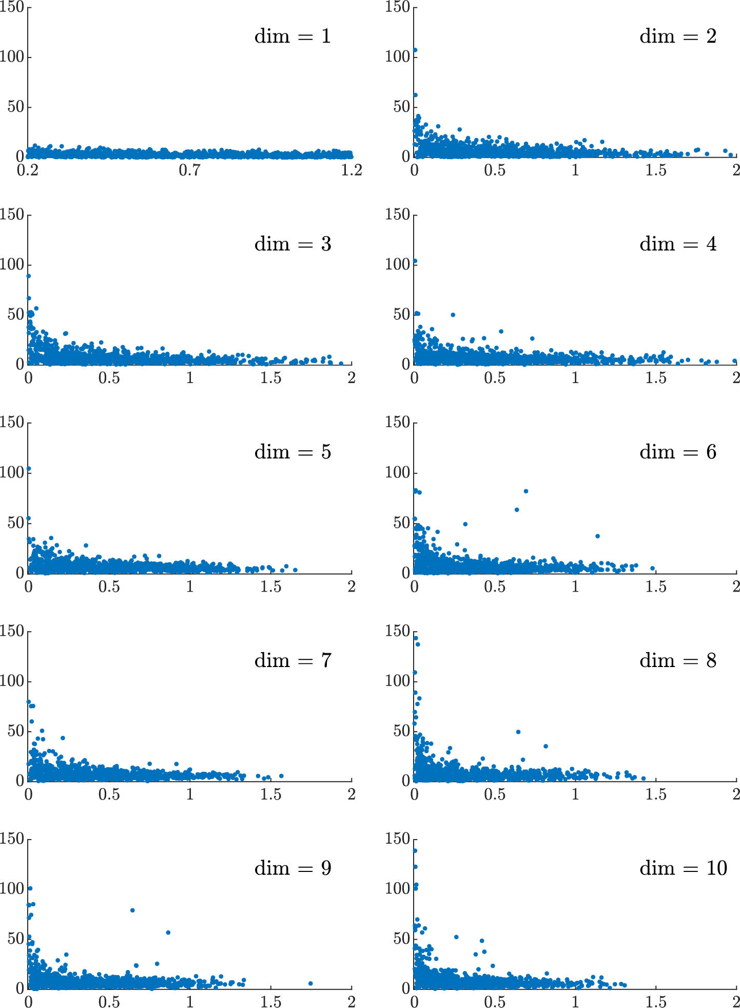
Figure 2: The scatter plot of $\min_{k}\{\left|\gamma_{r,{\bf A},k}\right|\}$ (x-axis) versus $e_{\bf K}$ (y-axis, in percentage) from dimension $1$ to $10$ for $t_{1}=1000$. The cases with $e_{\bf K}>150\%$ are not shown, but the chance of occurrence is below $1\%$.

Appendix D A Derivation of the Fokker-Planck Equation

We provide a proof of the Fokker-Planck equation Theorem 2.1 which will be generalized to derive an approximate Fokker-Planck equation Eq. 19.

By the stochastic Liouville equation, the dynamical equation of the probability density $P(x,t)$ is

$$\frac{\partial}{\partial t}P(x,t) =\frac{\partial}{\partial t}\langle\delta({\bf x}(t)-x)\rangle$$

$$=-\sum_{j}\frac{\partial}{\partial x_{j}}\langle\delta({\bf x}(t)-x)\frac{d{\bf x}_{j}}{dt}\rangle$$

$$=-\sum_{j}\frac{\partial}{\partial x_{j}}\langle\delta({\bf x}(t)-x)\sum_{k}{\bf A}_{jk}{\bf x}_{k}\rangle-\sum_{j,k}\frac{\partial}{\partial x_{j}}\langle\delta({\bf x}(t)-x)(\sqrt{2{\bf Q}})_{jk}{\bm{\xi}}_{k}\rangle$$

(22) $$=-\sum_{j,k}\frac{\partial}{\partial x_{j}}{\bf A}_{jk}x_{k}P(x,t)-\sum_{j,k}(\sqrt{2{\bf Q}})_{jk}\frac{\partial}{\partial x_{j}}\langle\delta({\bf x}(t)-x){\bm{\xi}}_{k}\rangle.$$

By the Furutsu-Donsker-Novikov correlation formula, we have

$$\langle{\bm{\xi}}_{k}\delta({\bf x}(t)-x)\rangle =\int_{0}^{t}\sum_{l}\langle{\bm{\xi}}_{k}(t){\bm{\xi}}_{l}(s)\rangle\langle\frac{\delta}{\delta{\bm{\xi}}_{l}(s)}\delta({\bf x}(t)-x)\rangle ds$$

$$=\int_{0}^{t}\delta(t-s)\langle\frac{\delta}{\delta{\bm{\xi}}_{k}(s)}\delta({\bf x}(t)-x)\rangle ds$$

(23) $$=-\int_{0}^{t}\delta(t-s)\sum_{l}\frac{\partial}{\partial x_{l}}\langle\delta({\bf x}(t)-x)\frac{\delta{\bf x}_{l}}{\delta{\bm{\xi}}_{k}(s)}\rangle ds.$$

Since ${\bf x}_{l}(t)={\bf x}_{l}(s)+\int_{s}^{t}f_{l}({\bf x}(t^{\prime}))+\sum_{k}(\sqrt{2{\bf Q}})_{lk}{\bm{\xi}}_{k}(t^{\prime})dt^{\prime}$, taking variation derivative on both sides, we have

$$\frac{\delta{\bf x}_{l}}{\delta{\bm{\xi}}_{p}(s)} =\int_{s}^{t}\sum_{m}{\bf A}_{lm}\frac{\delta{\bf x}_{m}}{\delta{\bm{\xi}}_{p}(s)}+\sum_{k}(\sqrt{2{\bf Q}})_{lk}\frac{\delta{\bm{\xi}}_{k}}{\delta{\bm{\xi}}_{p}(s)}dt^{\prime}$$

$$=\int_{s}^{t}\sum_{m}{\bf A}_{lm}\frac{\delta{\bf x}_{m}}{\delta{\bm{\xi}}_{p}(s)}+\sum_{k}(\sqrt{2{\bf Q}})_{lk}\delta_{kp}\delta(t^{\prime}-s)dt^{\prime}$$

$$=\int_{s}^{t}\sum_{m}{\bf A}_{lm}\frac{\delta{\bf x}_{m}}{\delta{\bm{\xi}}_{p}(s)}dt^{\prime}+(\sqrt{2{\bf Q}})_{lp},$$

where $\delta_{kl}$ is the Kronecker delta. Using the matrix notation, we have

$$\frac{\delta{\bf x}}{\delta{\bm{\xi}}}=e^{{\bf A}(t-s)}\sqrt{2{\bf Q}}.$$

Therefore, Appendix D becomes

$$\langle{\bm{\xi}}_{k}\delta({\bf x}(t)-x)\rangle =\int_{0}^{t}\delta(t-s)\sum_{l,m}\frac{\partial}{\partial x_{l}}\langle\delta({\bf x}(t)-x)\rangle(e^{{\bf A}(t-s)})_{lm}(\sqrt{2{\bf Q}})_{mk}ds$$

$$=\frac{1}{2}\sum_{l,m}\delta_{lm}(\sqrt{2{\bf Q}})_{mk}\frac{\partial}{\partial x_{l}}P(x,t)ds$$

(24) $$=\frac{1}{2}\sum_{l}(\sqrt{2{\bf Q}})_{lk}\frac{\partial}{\partial x_{l}}P(x,t),$$

where the last equality is due to the integration rule of the Dirac delta function and the fact that the matrix exponential becomes identity when $s=t$.

Inserting Appendix D to Appendix D, we obtain the classical Fokker-Planck equation,

$$\frac{\partial}{\partial t}P(x,t)=-\sum_{j,k}{\bf A}_{jk}\frac{\partial}{\partial x_{j}}x_{k}P(x,t)+\sum_{j,k}{\bf Q}_{jk}\frac{\partial^{2}}{\partial x_{j}\partial x_{k}}P(x,t).$$

Appendix E A Derivation of an Approximate Fokker-Planck Equation

We generalize the proof of the Fokker-Planck equation Eq. 19 to the case of a colored-noise driven process. The proof is based on [31, 32] in which approximate Fokker-Planck equations for the $1$-dimensional case were derived.

The dynamical equation of the probability density $P(x,t)$ reads

(25) $$\frac{\partial}{\partial t}P(x,t)=-\sum_{i,j}\frac{\partial}{\partial x_{i}}{\bf A}_{ij}x_{j}P(x,t)-\sum_{i,j}(\sqrt{2{\bf Q}})_{ij}\frac{\partial}{\partial x_{i}}\langle{\bm{\eta}}_{j}\delta({\bf x}(t)-x)\rangle.$$

As before, we have

$$\langle{\bm{\eta}}_{j}\delta(x(t)-x)\rangle =\int_{0}^{t}\sum_{k}\langle{\bm{\eta}}_{j}(t){\bm{\eta}}_{k}(s)\rangle\langle\frac{\delta}{\delta{\bm{\eta}}_{k}(s)}\delta({\bf x}(t)-x)\rangle ds$$

(26) $$=-\int_{0}^{t}\sum_{k}\langle{\bm{\eta}}_{j}(t){\bm{\eta}}_{k}(s)\rangle\sum_{l}\frac{\partial}{\partial x_{l}}\langle{\delta({\bf x}(t)-x)}\frac{\delta{\bf x}_{l}}{\delta{\bm{\eta}}_{k}(s)}\rangle ds.$$

First, we compute $\langle{\bm{\eta}}_{j}(t){\bm{\eta}}_{k}(s)\rangle$. For the initial condition ${\bm{\eta}}(0)$, the general solution of the noise processes can be written as

$${\bm{\eta}}_{j}(t)={\bm{\eta}}_{j}(0)e^{-\frac{t}{\tau}}+\frac{1}{\tau}\int_{0}^{t}e^{\frac{-(t-t^{\prime})}{\tau}}{\bm{\xi}}_{j}(t^{\prime})dt^{\prime}.$$

For $t>s\gg 0$, we compute

$$\langle{\bm{\eta}}_{j}(t){\bm{\eta}}_{k}(s)\rangle =\langle\big{(}{\bm{\eta}}_{j}(0)e^{\frac{-t}{\tau}}+\frac{1}{\tau}\int_{0}^{t}e^{\frac{-(t-t^{\prime})}{\tau}}{\bm{\xi}}_{j}(t^{\prime})dt^{\prime}\big{)}$$

$$\indent\indent\big{(}{\bm{\eta}}_{k}(0)e^{\frac{-s}{\tau}}+\frac{1}{\tau}\int_{0}^{s}e^{\frac{-(s-s^{\prime})}{\tau}}{\bm{\xi}}_{j}(s^{\prime})ds^{\prime}\big{)}\rangle$$

$$={\bm{\eta}}_{j}(0){\bm{\eta}}_{k}(0)e^{-(\frac{t+s}{\tau})}+\frac{1}{\tau^{2}}\int_{0}^{t}\int_{0}^{s}e^{-(\frac{t-t^{\prime}}{\tau})-(\frac{s-s^{\prime}}{\tau})}\langle{\bm{\xi}}_{j}(t^{\prime}){\bm{\xi}}_{k}(s^{\prime})\rangle dt^{\prime}ds^{\prime}$$

$$={\bm{\eta}}_{j}(0){\bm{\eta}}_{k}(0)e^{-(\frac{t+s}{\tau})}+\frac{1}{\tau^{2}}\int_{0}^{t}\int_{0}^{s}e^{-(\frac{t-t^{\prime}}{\tau})-(\frac{s-s^{\prime}}{\tau})}\delta(t^{\prime}-s^{\prime})\delta_{jk}dt^{\prime}ds^{\prime}$$

$$={\bm{\eta}}_{j}(0){\bm{\eta}}_{k}(0)e^{-(\frac{t+s}{\tau})}+\frac{\delta_{jk}}{\tau^{2}}\int_{0}^{s}e^{-(\frac{t-s^{\prime}}{\tau})-(\frac{s-s^{\prime}}{\tau})}ds^{\prime}$$

$$={\bm{\eta}}_{j}(0){\bm{\eta}}_{k}(0)e^{-(\frac{t+s}{\tau})}+\frac{\delta_{jk}}{2\tau}e^{-(\frac{t+s}{\tau})}\big{(}e^{\frac{2s}{\tau}}-1\big{)}$$

(27) $$\approx\frac{\delta_{jk}}{2\tau}e^{-(\frac{t-s}{\tau})}.$$

Next, the general solution for the stochastic process ${\bf x}(t)$ can be written as

$${\bf x}_{l}(t)={\bf x}_{l}(s)+\int_{s}^{t}f_{l}({\bf x}(t^{\prime}))+\sum_{m}(\sqrt{2{\bf Q}})_{lm}{\bm{\eta}}_{m}(t^{\prime})dt^{\prime}.$$

Hence, taking variational derivatives on both sides, we have

$$\frac{\delta{\bf x}_{l}}{\delta{\bm{\eta}}_{k}(s)} =\int_{s}^{t}\sum_{m}{\bf A}_{lm}\frac{\delta{\bf x}_{m}}{\delta{\bm{\eta}}_{k}(s)}+\sum_{m}(\sqrt{2{\bf Q}})_{lm}\frac{\delta{\bm{\eta}}_{m}}{\delta{\bm{\eta}}_{k}(s)}dt^{\prime}$$

$$=\int_{s}^{t}\sum_{m}{\bf A}_{lm}\frac{\delta{\bf x}_{m}}{\delta{\bm{\eta}}_{k}(s)}dt^{\prime}+\sum_{m}(\sqrt{2{\bf Q}})_{lm}\delta_{mk}$$

$$=\int_{s}^{t}\sum_{m}{\bf A}_{lm}\frac{\delta{\bf x}_{m}}{\delta{\bm{\eta}}_{k}(s)}dt^{\prime}+(\sqrt{2{\bf Q}})_{lk}.$$

Therefore, as before, we have

$$\frac{\delta{\bf x}}{\delta{\bm{\eta}}}=e^{{\bf A}(t-s)}\sqrt{2{\bf Q}}.$$

We use the eigen-decomposition of ${\bf A}$ to write down the exponential term entry-wise.

(28) $$(e^{{\bf A}(t-s)})_{lk}=\sum_{m}p_{m}^{lk}e^{\lambda_{m}(t-s)}.$$

Therefore, combining Appendices E, E, and 28, in the regime of $t\gg 0$, we have

$$\langle{\bm{\eta}}_{j}\delta({\bf x}(t)-x)\rangle \approx\int_{0}^{t}\sum_{k,l}\frac{\delta_{jk}}{2\tau}e^{-(\frac{t-s}{\tau})}\frac{\partial}{\partial x_{l}}\langle\delta({\bf x}(t)-x)\rangle\sum_{m,q}p_{m}^{lq}e^{\lambda_{m}(t-s)}(\sqrt{2{\bf Q}})_{qk}ds$$

$$=\int_{0}^{t}\sum_{l,m,q}(\sqrt{2{\bf Q}})_{qj}\frac{p_{m}^{lq}}{2\tau}e^{-(\frac{t-s}{\tau})+\lambda_{m}(t-s)}\frac{\partial}{\partial x_{l}}P(x,t)ds$$

$$=\sum_{q,l,m}\frac{p_{m}^{lq}(\sqrt{2{\bf Q}})_{qj}}{2\tau}\frac{\partial}{\partial x_{l}}P(x,t)\int_{0}^{t}e^{(\frac{-1}{\tau}+\lambda_{m})(t-s)}ds$$

(29) $$\approx-\sum_{q,l,m}\frac{p_{m}^{lq}(\sqrt{2{\bf Q}})_{qj}}{2(1-\tau\lambda_{m})}\frac{\partial}{\partial x_{l}}P(x,t),$$

since the dynamical matrix ${\bf A}$ has eigenvalues with negative real part.

Therefore, inserting Appendix E into Eq. Eq. 25, we obtain the approximate Fokker-Plank equation

$$\frac{\partial}{\partial t}P(x,t)=-\sum_{j,k}{\bf A}_{jk}\frac{\partial}{\partial x_{j}}x_{k}P(x,t)+\sum_{j,l}{\bf S}_{jl}\frac{\partial^{2}}{\partial x_{j}\partial x_{l}}P(x,t).$$

We remark that as the noise correlation time $\tau$ converges to $0$, the effective diffusion matrix ${\bf S}$ converges to the diffusion matrix ${\bf Q}$, and the approximate form (20) reduces to classical case. One can easily generalize to the case in which the noise correlation time depends on the coordinate $j$. To keep the argument simple, we do not pursuit the general formula.

References

- [1] G. Barrie Wetherill, P. Duncombe, M. Kenward, J. Köllerström, S. R. Paul, and B. J. Vowden. A review of multiple regression by least squares, pages 1–16. Springer Netherlands, Dordrecht, 1986.
- [2] C. Benedetti, M. G. A. Paris, and S. Maniscalco. Non-markovianity of colored noisy channels. Phys. Rev. A, 89:012114, Jan 2014.
- [3] S. Chapra. Applied Numerical Methods with MATLAB for Engineers and Scientists. McGraw-Hill Education, 2018.
- [4] R. Chartrand. Numerical differentiation of noisy, nonsmooth data. ISRN Applied Mathematics, 2011:164564, May 2011.
- [5] B. Cui and A. Zaccone. Generalized langevin equation and fluctuation-dissipation theorem for particle-bath systems in external oscillating fields. Phys. Rev. E, 97:060102, Jun 2018.
- [6] W.-L. Duan and H. Fang. The unified colored noise approximation of multidimensional stochastic dynamic system. Physica A: Statistical Mechanics and its Applications, 555:124624, 2020.
- [7] G. Falsone. Stochastic differential calculus for gaussian and non-gaussian noises: A critical review. Communications in Nonlinear Science and Numerical Simulation, 56:198–216, 2018.
- [8] J. P. Gonzalez, J. C. Neu, and S. W. Teitsworth. Experimental metrics for detection of detailed balance violation. Phys. Rev. E, 99:022143, Feb 2019.
- [9] G. Gradziuk, G. Torregrosa, and C. P. Broedersz. Irreversibility in linear systems with colored noise. Phys. Rev. E, 105(2):024118–10, 2022.
- [10] F. Hassanibesheli, N. Boers, and J. Kurths. Reconstructing complex system dynamics from time series: a method comparison. New Journal of Physics, 22(7):073053, jul 2020.
- [11] P. Jung and P. Hänggi. Dynamical systems: A unified colored-noise approximation. Phys. Rev. A, 35:4464–4466, May 1987.
- [12] P. Jung and H. Risken. Motion in a double-well potential with additive colored gaussian noise. Zeitschrift für Physik B Condensed Matter, 61(3):367–379, Sep 1985.
- [13] D. Kondrashov, M. D. Chekroun, and M. Ghil. Data-driven non-markovian closure models. Physica D: Nonlinear Phenomena, 297:33–55, 2015.
- [14] S. Kravtsov, D. Kondrashov, and M. Ghil. Multilevel regression modeling of nonlinear processes: Derivation and applications to climatic variability. Journal of Climate, 18(21):4404–4424, 2005.
- [15] F. Kwasniok. Linear inverse modeling of large-scale atmospheric flow using optimal mode decomposition. Journal of the Atmospheric Sciences, 79(9):2181–2204, 2022.
- [16] M. M. Kłosek-Dygas, B. J. Matkowsky, and Z. Schuss. Colored noise in dynamical systems. SIAM Journal on Applied Mathematics, 48(2):425–441, 1988.
- [17] C. Martinez-Villalobos, D. J. Vimont, C. Penland, M. Newman, and J. D. Neelin. Calculating state-dependent noise in a linear inverse model framework. Journal of the Atmospheric Sciences, 75:479–496, 2017.
- [18] P. McCullagh. Generalized Linear Models. CRC Press, 2019.
- [19] G. N. Mil’shtein. A method of second-order accuracy integration of stochastic differential equations. Theory of Probability & Its Applications, 23(2):396–401, 1979.
- [20] M. Niemann, T. Laubrich, E. Olbrich, and H. Kantz. Usage of the Mori-Zwanzig method in time series analysis. Phys Rev E Stat Nonlin Soft Matter Phys, 77(1 Pt 1):011117, Jan 2008.
- [21] B. Øksendal. Stochastic differential equations : an introduction with applications. Journal of the American Statistical Association, 82:948, 1987.
- [22] C. Penland. Random forcing and forecasting using principal oscillation pattern analysis. Monthly Weather Review, 117(10):2165–2185, 1989.
- [23] C. Penland and T. Magorian. Prediction of niño 3 sea surface temperatures using linear inverse modeling. Journal of Climate, 6(6):1067–1076, 1993.
- [24] C. Penland and L. Matrosova. A balance condition for stochastic numerical models with application to the el niño-southern oscillation. Journal of Climate, 7(9):1352–1372, 1994.
- [25] H. Risken. The Fokker-Planck equation, volume 18 of Springer Series in Synergetics. Springer-Verlag, Berlin, second edition, 1989. Methods of solution and applications.
- [26] D. T. Schmitt and M. Schulz. Analyzing memory effects of complex systems from time series. Phys. Rev. E, 73:056204, May 2006.
- [27] U. Seifert. Stochastic thermodynamics, fluctuation theorems and molecular machines. Reports on Progress in Physics, 75(12):126001, nov 2012.
- [28] S.-I. Shin, P. D. Sardeshmukh, M. Newman, C. Penland, and M. A. Alexander. Impact of annual cycle on enso variability and predictability. Journal of Climate, 34(1):171–193, 2021.
- [29] J. J. Stickel. Data smoothing and numerical differentiation by a regularization method. Computers & Chemical Engineering, 34(4):467–475, 2010.
- [30] S. Särkkä and A. Solin. Applied Stochastic Differential Equations. Institute of Mathematical Statistics Textbooks. Cambridge University Press, 2019.
- [31] D. Wu, X. Luo, and S. Zhu. Stochastic system with coupling between non-gaussian and gaussian noise terms. Physica A: Statistical Mechanics and its Applications, 373:203–214, 2007.
- [32] H. Zhang, W. Xu, and Y. Xu. The study on a stochastic system with non-gaussian noise and gaussian colored noise. Physica A: Statistical Mechanics and its Applications, 388(6):781–788, 2009.
- [33] H. Zhivomirov. A method for colored noise generation. Romanian journal of acoustics and vibration, 15(1):14–19, 2018.