Advancing Parameter Efficiency in Fine-tuning via Representation Editing

Abstract

Parameter Efficient Fine-Tuning (PEFT) has gained significant attention for its ability to achieve competitive results while updating only a small subset of trainable parameters. Despite the promising performance of current PEFT methods, they present challenges in hyperparameter selection, such as determining the rank of LoRA or Adapter, or specifying the length of soft prompts. In addressing these challenges, we propose a novel approach to fine-tuning neural models, termed Representation EDiting (RED), which scales and biases the representation produced at each layer. RED substantially reduces the number of trainable parameters by a factor of $25,700$ compared to full parameter fine-tuning, and by a factor of $32$ compared to LoRA. Remarkably, RED achieves comparable or superior results to full parameter fine-tuning and other PEFT methods. Extensive experiments were conducted across models of varying architectures and scales, including RoBERTa, GPT-2, T5, and Llama-2, and the results demonstrate the efficiency and efficacy of RED, positioning it as a promising PEFT approach for large neural models.

Advancing Parameter Efficiency in Fine-tuning via Representation Editing

Muling Wu, Wenhao Liu, Xiaohua Wang, Tianlong Li, Changze Lv Zixuan Ling, Jianhao Zhu, Cenyuan Zhang, Xiaoqing Zheng, Xuanjing Huang School of Computer Science, Fudan University, Shanghai, China {mlwu22,whliu22,xiaohuawang22,tlli22,czlv22}@m.fudan.edu.cn {zhengxq,xjhuang}@fudan.edu.cn

1 Introduction

Pre-training on large-scale unlabeled datasets and then fine-tuning on task-specific datasets has led to significant improvements across various natural language processing (NLP) tasks and has emerged as the predominant training paradigm Devlin et al. (2018); Raffel et al. (2020); Radford et al. (2018). However, performing full parameter fine-tuning for each task would be prohibitively expensive with the growing model scale Brown et al. (2020). For example, BERT consists of up to $220$ million parameters; T5 comprises up to $11$ billion parameters and GPT-3 contains up to $175$ billion parameters. In this context, how to efficiently and effectively adapt large models to particular downstream tasks is an intriguing research issue He et al. (2021).

To address this issue, researchers have proposed three main lines of Parameter Efficient Fine-Tuning (PEFT) methods Ding et al. (2022). Specifically, additional-based methods introduce extra trainable neural modules or parameters that do not exist in the original model Houlsby et al. (2019); Karimi Mahabadi et al. (2021); Li and Liang (2021a); Lester et al. (2021a). Specification-based methods specify certain parameters in the original model become trainable, while others are frozen Zaken et al. (2021); Guo et al. (2020). Reparameterization-based methods reparameterize trainable parameters to a parameter-efficient form by transformation Hu et al. (2021); Zhang et al. (2023a); Ding et al. (2023).

Among these PEFT methods, Low-Rank Adaptation (LoRA) is considered one of the most efficient methods at present and its efficacy has been empirically validated across diverse models of varying scales. Despite its excellent performance, it still requires a considerable amount of trainable parameters. According to Aghajanyan et al. (2020) and Kopiczko et al. (2023), the upper bound for intrinsic dimensions is much smaller than what is typically utilized in such methods. For instance, the ${d}_{90}$ for RoBERTa base is reported to be $896$. Still, when utilizing LoRA to fine-tune this model, the number of trainable parameters reaches $0.3$M, suggesting that the parameter count could be reduced further.

In addition, although previous works Mao et al. (2021); He et al. (2021); Ding et al. (2022) have attempted to design different lightweight module structures or insert these modules into different positions in the base model, these PEFT methods consider fine-tuning the model from the perspective of adjusting model weights, which leads to many inconveniences in the selection of hyperparameters, such as the rank of LoRA and Adapter, as well as the length of Soft Prompt and Prefix.

Inspired by the idea of representation engineering Zou et al. (2023) representation can be modified to steer model outputs toward specific concepts and change the model’s behavior. We hypothesize that we can also consider fine-tuning the model from the perspective of editing neural network representations, leading to our proposed Representation EDiting (RED) approach. Instead of focusing on neurons and their connections, we fine-tune the model by learning a group of “edit vectors” to directly edit the representations of each layer and freezing the base model parameters, as shown in figure 1 (b).

Moreover, RED is highly parameter efficient. Using Llama-2 7B as an example, we show that RED can still achieve very promising performance by adjusting only $0.26$M parameters, which is $25,700$ times less than full parameter fine-tuning, making it both storage- and compute-efficient.

The contribution of this study can be summarized as follows:

• We consider fine-tuning the model from a new perspective of directly modifying the model representation, which is different from the previous work that adjusted the model weight, and propose our PEFT method, Representation EDiting (RED).

• We conducted extensive experiments on models with different structures and scales, including RoBERTa, GPT-2, T5, and Llama-2, and validated the effectiveness of RED on a series of NLU and NLG tasks although it only requires a small number of trainable parameters, and is quite simple to implement.

• We perform the ablation study to better understand the individual components of RED and their effects on performance.

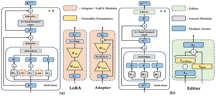
Figure 1: Comparison of previous PEFT methods and our proposed RED. Left: LoRA introduces the learnable bottleneck-shaped modules (orange area) through parallel connections for the $\mathbf{W}_{q}$ and $\mathbf{W}_{v}$ matrices of attention blocks, and models the weight changes of these two matrices in a low-rank manner. Adapter introduces learnable modules with similar structures (orange area) through serial connections after the attention sub-layers and feed-forward sub-layers to train the model. Right: RED introduces two learnable vectors $l_{scaling}$ and $l_{bias}$ directly modifies the representation (green area) after feed-forward sub-layer to fine-tune the model.

2 Related Work

Ding et al. (2022) categorize the PEFT methods into three groups according to the operations on the learnable parameters: addition-based, specification-based, and reparameterization-based methods.

Addition-based methods introduce additional components for training based on the foundation model. Specifically, Houlsby et al. (2019); Stickland and Murray (2019); Karimi Mahabadi et al. (2021) and Rücklé et al. (2020) inject learnable bottleneck neural modules to the transformer layers. Brown et al. (2020) and Shin et al. (2020) found that by concatenating some discrete tokens before the input text, the performance of the model can be improved without updating parameters. However, manually designing prompts requires a lot of effort, and the optimization problem in discrete space is relatively more difficult. Therefore, the subsequent works Lester et al. (2021b); Li and Liang (2021b); Wu et al. (2023); Wang et al. (2023) replace these discrete tokens with continuous vectors in front of the embedding layer or various hidden layers, also known as soft prompts, and optimize them through simple gradient descent.

Specification-based methods do not introduce any new parameters in the model, and they sparsely select part of the foundation model parameters for adjustment and freeze other parameters. Among them, Lee et al. (2019) adjusts the model parameters of the last few layers of BERT and RoBERTa. BitFit Ben-Zaken et al. (2021) fine-tunes the model by only optimizing the bias terms inside the model. Unlike both of these methods, which manually specify the parameters that need to be adjusted in the network, Guo et al. (2020) and Zhao et al. (2020) use the learnable mask to dynamically select the parameters that need to be adjusted.

Reparameterization-based methods transform the optimization process of trainable parameters into a low-dimensional subspace. LoRA Hu et al. (2021) proposes to employ low-rank matrices to approximate the weight changes during fine-tuning. QLoRA Dettmers et al. (2023) combines low-rank adaptation with model quantization to further reduce storage usage during the model fine-tuning process. AdaLoRA Zhang et al. (2023b) proposes using SVD decomposition to approximate the changes in weights, which allocate more trainable parameters to more important weight matrices, resulting in better performance.

In addition, IA3 Liu et al. (2022) and VeRA Kopiczko et al. (2023) also consider scaling vectors in their implementation. However, IA3 not only needs to adjust the key vectors and value vectors of the attention module, as well as the vectors of the projection matrix but also needs to introduce additional complex loss functions. VeRA still needs to introduce a randomly initialized LoRA matrix and adjust the vectors passing through the projection matrix under LoRA. Compared to them, RED is much simpler in implementation, as it only needs to directly edit the model’s representations.

In the domain of computer vision, Lian et al. (2022) presented a similar method, called SSF, yet our investigation diverges in several key aspects. Specifically, SSF needs to adjust the feature vectors across nearly all transformer layers, including multi-head attention, MLP, and layer normalization components. Consequently, the size of parameters adjusted in their method approximates those manipulated in other PEFT techniques, such as Adapter and VPT Jia et al. (2022). In contrast, our RED method draws inspiration from the emerging field of representation engineering, necessitating only the alteration of activation patterns produce by FFN sub-layers, which constitute a much less proportion of the entire network’s architecture. While SSF achieves a reduction in the number of fine-tuning parameters by a factor of $300$ compared to original models, RED accomplishes a reduction by approximately $25,700$ times. Furthermore, SSF’s evaluation was limited to a narrow range of simple image classification tasks using relatively small models (under $100$M parameters), whereas RED has proven its effectiveness across a range of natural language understanding and generation tasks, employing significantly larger models of up to $7$B parameters. Our ablation studies further reveal that manipulations of layers other than the FFN sub-layers are undesired and extraneous, leading either to diminished efficiency in parameter fine-tuning or to reduced performance outcomes.

Representation engineering Zou et al. (2023) suggests that neural representations are becoming more well-structured and place representations and transformations between them at the center of analysis rather than neurons or circuits. Specifically, Liu et al. (2023) points out that neural network weights determine neural activity, neural activity determines the networks’ output, and the networks’ output determines the networks’ behavior and utilizes this feature to operate in the representation space and achieves model alignment. Turner et al. (2023) adds a “steer vector” to the representation of each hidden layer during inference time to control the sentiment and style of the model output. Subramani et al. (2022) also extracted these “steel vectors” in the hidden space and completed unsupervised text style transfer by modifying the hidden representation through these vectors.

3 Method

In this section, we briefly review previous methods and introduce Representation EDiting (RED), a novel parameter effective fine-tuning method that adapts pre-trained models to downstream tasks by directly modifying model representations.

3.1 Recap of previous PEFT methods

The transformer model Vaswani et al. (2017) is now the cornerstone architecture behind most state-of-the-art PLMs. Transformer models are composed of $L$ stacked blocks, where each block contains two types of sub-layers: multi-head self-attention and fully connected feed-forward network (FFN). Except for the prompt-based methods which introduce learnable parameters in the embedding layer, many other PEFT methods are trained based on these two sub-layers.

Figure 1 (a) shows two commonly used PEFT methods, Adapter and LoRA. Except for a few additional parameters that need to be trained, the parameters of the pre-trained model are frozen.

Specifically, LoRAHu et al. (2021) introduces the learnable bottleneck-shaped modules through parallel connections for the $\mathbf{W}_{q}$ and $\mathbf{W}_{v}$ matrices of attention blocks and models the weight changes of these two matrices in a low-rank manner. For a pre-trained weight matrix $\mathbf{W}\in\mathbb{R}^{d\times k}$, LoRA represents its update with two low-rank decomposition matrices: $\mathbf{W}+\Delta{W}=\mathbf{W}+{s}\cdot\mathbf{W}_{down}\mathbf{W}_{up}$, where $\mathbf{W}_{down}\in\mathbb{R}^{d\times r}$, $\mathbf{W}_{up}\in\mathbb{R}^{r\times k}$ and $s$ is the scaling scalar, which is a hyperparameter set in advance. For ${h}={x}\mathbf{W}$, LoRA modified forward pass yields:

$${h}={x}\mathbf{W}+s\cdot{x}\mathbf{W}_{down}\mathbf{W}_{up}$$ (1)

The initial adapter Houlsby et al. (2019) inserts trainable adapter modules between transformer sub-layers. The adapter module contains a down-projection matrix $\mathbf{W}_{down}\in\mathbb{R}^{d\times r}$, map input ${h}_{1}\in\mathbb{R}^{d}$ to a low dimensional space of the specified dimension $r$. This vector is restored to its original dimension $d$ through a nonlinear activation function $f(\cdot)$ and an up-projection matrix $\mathbf{W}_{up}\in\mathbb{R}^{r\times d}$. The residual structure is also applied in the adapter and the output ${h}_{2}\in\mathbb{R}^{d}$ of this module is obtained, formalized as:

$${h}_{2}={h}_{1}+f({h}_{1}\mathbf{W}_{down})\mathbf{W}_{up}$$ (2)

Pfeiffer et al. (2020) have proposed a more efficient adapter variant that is inserted only after the FFN sub-layer.

3.2 Representation Editing

Previous PEFT methods fine-tune pre-trained models from the perspective of adjusting model weights, which poses challenges for the selection of hyperparameters. For example, choosing a suitable rank for the Adapter or LoRA module can be troublesome. A conservative choice of huge rank $r$ can waste training time and computation resources, while progressively setting $r$ tiny may degrade model performance and lead to from-scratch re-training Ding et al. (2023).

Turner et al. (2023) explicitly control the output behavior of the model by adding a “steer vector” to the hidden layer at inference time in a non-parametric way, and we think that model training can also be controlled through a set of similar “edit vectors”. Inspired by this idea, we propose a new PEFT method to fine-tune the model by directly modifying the representation with two learnable vectors, as shown in Figure 1 (b).

Specifically, we first introduce a learnable scaling vector $l_{scaling}\in\mathbb{R}^{d}$ and employ it to perform the Hadamard product with the representation vector ${h}_{1}$, scaling the features of each dimension in ${h}_{1}$ through element-wise multiplication. Additionally, we introduce another learnable bias vector $l_{bias}\in\mathbb{R}^{d}$. Adding this bias vector $l_{bias}$ and scaled vector to obtain the output $h_{2}$, which is formalized as:

$$h_{2}=l_{scaling}\odot h_{1}+l_{bias}$$ (3)

,where $\odot$ denotes element-wise multiplication (Hadamard product), $h_{1}\in\mathbb{R}^{d}$ is the unmodified representation and $h_{2}\in\mathbb{R}^{d}$ is the modified representation.

In addition, we initialize the scaling vector $l_{scaling}$ to one vector and the bias vector $l_{bias}$ to zero vectors, which ensures that the representation of the model does not change too much when these “edit vectors” are first added.

Model & Method	# Params.	MNLI	SST-2	MRPC	CoLA	QNLI	QQP	RTE	STS-B	Avg.
FT (base)	$125\mathbf{M}$	$87.3$	$94.4$	$87.9$	$62.4$	$92.5$	$91.7$	$78.3$	$90.6$	$85.6$
Adapter (base)	$0.4\mathbf{M}$	$87.0$	$93.3$	$88.4$	$60.9$	$92.5$	$90.5$	$76.5$	$90.5$	$85.0$
LoRA (base)	$0.3\mathbf{M}$	$86.6$	$93.9$	$88.7$	$59.7$	$92.6$	$90.4$	$75.3$	$90.3$	$84.7$
Adapter_FFN (base)	$0.3\mathbf{M}$	$87.1$	$93.0$	$88.8$	$58.5$	$92.0$	$90.2$	$77.7$	$90.4$	$84.7$
BitFit (base)	$0.1\mathbf{M}$	$84.7$	$94.0$	$88.1$	$54.0$	$91.0$	$87.3$	$69.8$	$89.5$	$82.3$
RED (base)	$0.02\mathbf{M}$	$83.9$	$93.9$	$89.2$	$61.0$	$90.7$	$87.2$	$78.0$	$90.4$	$84.3$
FT (large)	$355\mathbf{M}$	$88.8$	$96.0$	$91.7$	$68.2$	$93.8$	$91.5$	$85.8$	$92.6$	$88.5$
Adapter (large)	$0.9\mathbf{M}$	$90.1$	$95.2$	$90.5$	$65.4$	$94.6$	$91.4$	$85.3$	$91.5$	$88.0$
LoRA (large)	$0.8\mathbf{M}$	$90.2$	$96.0$	$89.8$	$65.5$	$94.7$	$90.7$	$86.3$	$91.7$	$88.1$
Adapter_FFN (large)	$0.8\mathbf{M}$	$90.3$	$96.1$	$90.5$	$64.4$	$94.3$	$91.3$	$84.8$	$90.2$	$87.7$
RED (large)	$0.05\mathbf{M}$	$89.5$	$96.0$	$90.3$	$68.1$	$93.5$	$88.8$	$86.2$	$91.3$	$87.9$

Table 1: RoBERTa base and RoBERTa large with RED and other adaptation methods on the GLUE benchmark. Higher is better for all metrics and fewer is better for the number of trainable parameters. The standard deviations of results from different methods are shown in Table 14 in Appendix C.

4 Experiments

In this section, we conduct a series of experiments to evaluate our PEFT method. We evaluate the downstream task performance of RED on RoBERTa Liu et al. (2019), T5 Raffel et al. (2020), GPT-2 Radford et al. (2019) and large scale language model Llama-2 Touvron et al. (2023). Our experiments cover a wide range of tasks, from natural language understanding (NLU) to generation (NLG). Specifically, we evaluate our methods on the GLUE Wang et al. (2018) benchmark for RoBERTa and T5 like Hu et al. (2021) and Asai et al. (2022). We follow the setup of Li and Liang (2021a) and Hu et al. (2021) on GPT-2 for a direct comparison. What’s more, we conducted instruction tuning experiments on Llama-2 using the UltraFeedback Cui et al. (2023) dataset to further test the applicability of these adaptation methods on large-scale language models. See Appendix A for more details on the datasets and evaluation metrics we use.

4.1 Baselines

To fully and fairly compare with other baselines, we reproduce prior PEFT methods according to their work settings and also reuse the numbers provided in their articles. We compare RED to the following baselines:

Fine-Tuning (FT) is a very common method for training models that updates all model parameters using gradient descent. Lee et al. (2019) proposes a variant of FT, which simply updates some layers and freezes other layers. We include one such baseline reported in prior work Li and Liang (2021a) on GPT-2, which adapts just the last two layers $(\mathbf{FT^{top2}})$.

Bias-terms Fine-tuning (BitFit) freezes most of the transformer parameters and trains only the bias-terms, referred to Ben-Zaken et al. (2021).

Adapter adds the learnable lightweight module adapter between the sub-layers of the transformer. During forward propagation, the input is sequentially processed by sub-layers of the pre-trained models and these adapters to obtain the final output. However, during backpropagation, only these adapters obtain gradient to update parameters, while the other parameters of the model remain fixed and unchanged, referred to Houlsby et al. (2019).

Adapter_FFN is one kind of variant of Adapter proposed by Pfeiffer et al. (2020). Unlike the initial Adapter that requires inserting the learnable module between all sub-layers, Adapter_FFN only needs to apply an adapter after each FFN sub-layer.

AdapterDrop is another variant of Adapter proposed by Rücklé et al. (2020), which drops some adapter layers for greater efficiency.

Low-Rank Adaption(LoRA) performs low-rank decomposition on the incremental matrix $\Delta W$ and models the weight changes by multiplying two low-rank matrices. These two learnable matrices are concatenated in parallel next to the pre-trained model matrix, and they simultaneously process the input and add up the computation results as the output of this block, referred to Hu et al. (2021).

Prompt Tuning(PT) prefixes some continuous vectors at the embedding layer, which are learnable and are generally not in the model’s vocabulary, referred to Lester et al. (2021b).

Prefix tuning is a general version of prompt tuning, which prepends the continuous vectors at each hidden state, and these continuous vectors participate in the calculation of attention as key vectors and value vectors, referred to Li and Liang (2021b).

Model & Method	# Params.	BLEU	NIST	MET	ROUGE-L	CIDEr
FT (medium)	$355\mathbf{M}$	$65.95$	$8.52$	$45.95$	$69.13$	$2.35$
$\mathbf{FT^{top2}}$ (medium)	$25.2\mathbf{M}$	$65.94$	$8.53$	$44.28$	$68.83$	$2.23$
Adapter (medium)	$0.9\mathbf{M}$	$64.31$	$8.29$	$44.91$	$67.72$	$2.28$
LoRA (medium)	$0.8\mathbf{M}$	$67.43$	$8.65$	$46.01$	$69.64$	$2.42$
Adapter_FFN (medium)	$0.8\mathbf{M}$	$64.41$	$8.30$	$44.74$	$67.53$	$2.29$
Prefix Tuning (medium)	$0.8\mathbf{M}$	$63.92$	$8.26$	$41.81$	$66.86$	$2.03$
RED (medium)	$0.05\mathbf{M}$	$64.86$	$8.36$	$44.99$	$67.62$	$2.28$
FT (large)	$774\mathbf{M}$	$65.56$	$8.50$	$45.40$	$68.38$	$2.27$
Adapter (large)	$1.8\mathbf{M}$	$65.94$	$8.46$	$45.78$	$68.65$	$2.34$
LoRA (large)	$1.5\mathbf{M}$	$68.24$	$8.76$	$46.23$	$69.92$	$2.42$
Adapter_FFN (large)	$1.5\mathbf{M}$	$65.53$	$8.41$	$45.65$	$68.46$	$2.33$
Prefix Tuning (large)	$1.5\mathbf{M}$	$65.50$	$8.45$	$43.97$	$67.32$	$2.23$
RED (large)	$0.09\mathbf{M}$	$65.77$	$8.42$	$46.12$	$69.03$	$2.36$

Table 2: GPT-2 medium and large with RED and other adaptation methods on the E2E NLG Challenge. Higher is better for all metrics and fewer is better for the number of trainable parameters. The standard deviations of results from different methods are shown in Table 15 in Appendix C.

4.2 RoBERTa base/large

We take the pre-trained RoBERTa base (125M) and RoBERTa large (355M) from the HuggingFace Transformers library Wolf et al. (2019) and evaluate the performance of different efficient adaptation approaches on tasks from the GLUE benchmark, which is a widely recognized benchmark for natural language understanding. Moreover, we also replicate prior work according to their setup and conduct experiments under fair and reasonable configuration, see Appendix B.1 for more details of the hyperparameter used in our experiments.

Unlike previous works Liu et al. (2019); Hu et al. (2021) that use the best model checkpoint on the MNLI dataset to initial model when dealing with MRPC, RTE, and STS-B to boost the performance, we consider a more general setting that trains the model from scratch.

The experimental performance of RED, as well as other adaption methods, is recorded in Table 1. Our results indicate that RED is comparable to other PEFT methods, which underlines the validity of directly editing representation as a feasible solution to adapt pre-trained models to downstream tasks.

RED has demonstrated strong competitiveness on training datasets with a data size of less than $100$k, such as being able to match or even surpass other PEFT methods on SST-2, MRPC, CoLA, STS-B, and RTE. For datasets with data sizes greater than $100$k, such as MNLI, QQP, and QNLI, the performance of BitFit and RED, which have the smallest number of trainable parameters, is slightly lower than other baselines. We think that larger-scale training datasets may require more trainable parameters to adapt.

Moreover, RED is highly parameter efficient. It can still maintain very good performance even with $7,200$ times less trainable parameters than full parameter fine-tuning and $16$ times less trainable parameters than LoRA, indicating that there is still room for improvement to further reduce the number of trainable parameters even if prior works adopt very sparse network structures to achieve this goal, which is consistent with the conclusions found by Aghajanyan et al. (2020) and Kopiczko et al. (2023).

Model & Method	# Params.	MNLI	SST-2	MRPC	CoLA	QNLI	QQP	RTE	STS-B	Avg.
FT (base)*	$220\mathbf{M}$	$86.8$	$94.6$	$90.2$	$61.8$	$93.0$	$91.6$	$71.9$	$89.7$	$84.9$
Adapter (base)*	$1.9\mathbf{M}$	$86.5$	$93.8$	$85.3$	$64.0$	$93.2$	$90.2$	$71.9$	$90.7$	$84.5$
AdapterDrop (base)*	$1.1\mathbf{M}$	$86.3$	$93.6$	$86.3$	$62.7$	$93.2$	$90.2$	$71.2$	$91.4$	$84.4$
BitFit (base)*	$0.3\mathbf{M}$	$85.3$	$94.2$	$86.8$	$58.2$	$93.0$	$90.1$	$67.6$	$90.9$	$83.3$
PT (base)*	$0.08\mathbf{M}$	$81.3$	$90.9$	$68.1$	$10.6$	$92.8$	$89.7$	$54.7$	$89.5$	$72.2$
RED (base)	$0.04\mathbf{M}$	$85.9$	$93.0$	$91.7$	$61.1$	$91.2$	$89.2$	$72.7$	$88.2$	$84.1$

Table 3: T5 base with RED and other adaptation methods on the GLUE benchmark. Higher is better for all metrics and fewer is better for the number of trainable parameters. * indicates numbers published in prior works.

4.3 GPT-2 medium/large

In addition to natural language understanding tasks, we also conduct experiments on natural language generation tasks. We take the pre-trained GPT-2 medium (355M) and GPT-2 large (774M) from the HuggingFace Transformers library and evaluate these methods on E2E NLG Challenge Novikova et al. (2017). What’s more, we replicate prior works according to the setup of Li and Liang (2021a) and Hu et al. (2021), see Appendix B.2 for more details of the hyperparameter used in our experiments.

The experimental performance of RED, as well as other adaption methods, is recorded in Table 2. Our experimental results indicate that RED achieved comparable performance with other baselines in various metrics of the E2E NLG Challenge, proving that adapting downstream tasks through editing representation not only works on classification tasks but also performs well on generation tasks.

Similarly, RED achieves excellent performance with much less trainable parameters. In section 5.3, we set the rank of LoRA and Adapter to 1. At this point, the performance of RED is better than these PEFT methods, proving that RED is not only parameter efficient but also parameter effective.

4.4 T5

To further verify the universality of RED, we also select the encoder-decoder architecture model for experiments. Specifically, we take the pre-trained T5-base (220M) from the HuggingFace Transformers library and evaluate these methods on GLUE BenchMark. We reuse the results provided by Asai et al. (2022) and conduct experiments based on similar settings, see Appendix B.3 for more details of the hyperparameter used in our experiments.

The experimental performance of RED, as well as other adaption methods, is recorded in Table 3. Compared with other baselines, RED still achieved comparable results on T5 even with fewer parameter adjustments, indicating its universality and versatility for various model architectures.

RED demonstrated a significant performance advantage when compared to the PEFT method of Prompt Tuning, which has a similar number of trainable parameters. To be specific, RED surpasses Prompt Tuning by $11.9$ points, indicating that allocating a small number of learnable parameters at each layer to edit representation is a more appropriate approach compared to allocating all learnable parameters on the embedding layer of the model.

4.5 Llama-2

Lastly, we scale up to Llama-2 with $7$ billion parameters to verify the feasibility of applying RED on large-scale language models. Specifically, we selected Llama-2 (7B) as the base model and utilized full parameter fine-tuning, LoRA, and RED to fine-tune the model on UltraFeedback Cui et al. (2023) respectively. As for evaluation, we assessed the performance of these different methods across three widely used benchmarks: Open LLM LeaderboardBeeching et al. (2023), AlpacaEval Li et al. (2023), and MT-Bench Zheng et al. (2023). See Appendix B.4 for more details of the hyperparameter used in our experiments.

Method	# Params.	AlpacaEval (win %)
FT	$6739\mathbf{M}$	$80.93$
LoRA	$8.39\mathbf{M}$	$81.48$
RED	$0.26\mathbf{M}$	$81.69$

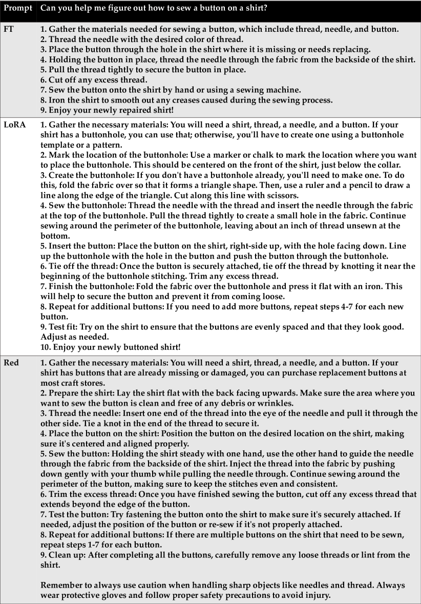
Figure 3: Response from RED provides a comprehensive, step-by-step guide that is detailed and methodical, ensuring that even beginners can follow along easily. It covers preparation, threading, placement, sewing technique, and cleanup, offering safety tips and encouraging testing for security. Conversely, the response from LoRA focuses incorrectly on creating buttonholes rather than sewing buttons, which might confuse readers seeking to attach buttons. Response from FT offers a simplified overview but lacks the depth and clarity of RED, making it less instructive for those unfamiliar with sewing. RED’s detailed approach ensures accuracy and success in sewing a button.

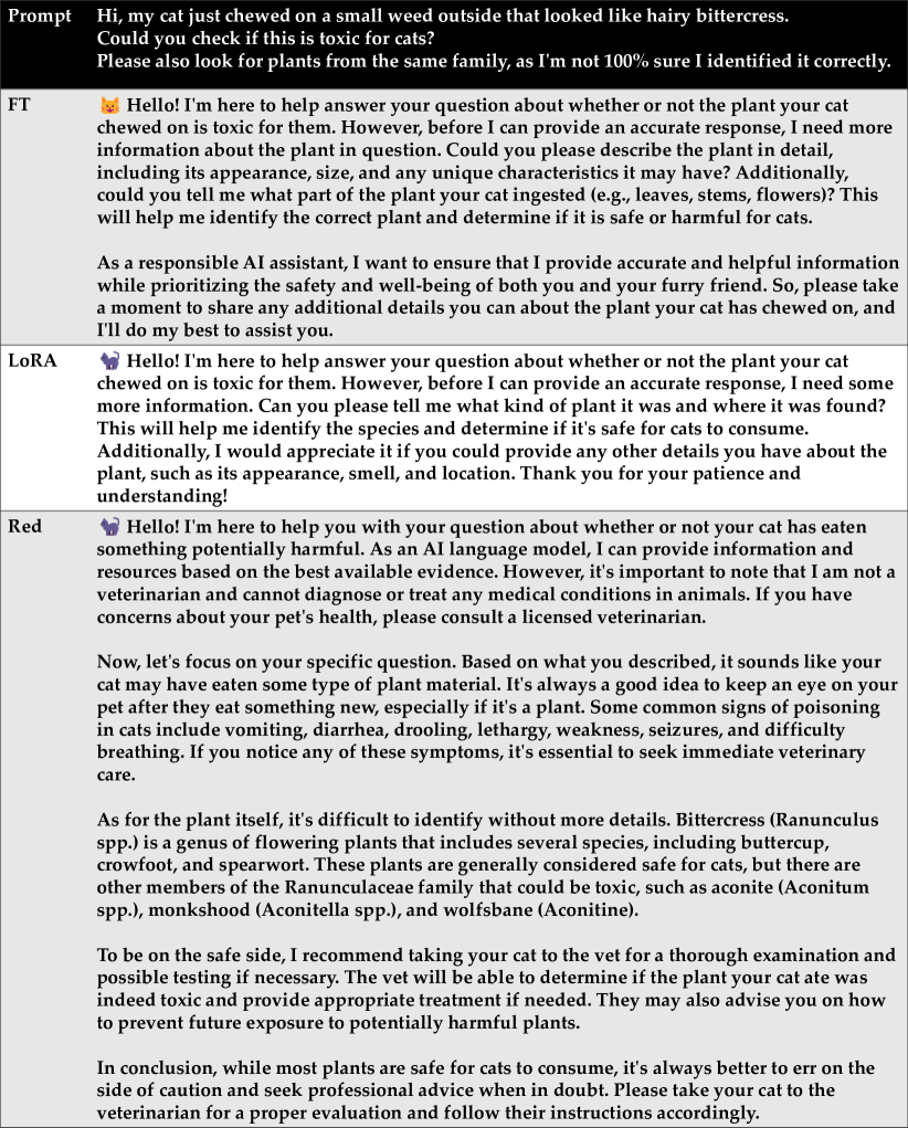
Figure 4: Response from RED offers a comprehensive and proactive approach, addressing immediate concerns, potential symptoms to watch for, and the importance of veterinary consultation. It provides a general safety assessment of the Ranunculaceae family, including possible toxic members, emphasizing the need for professional evaluation. This response balances informative content with practical advice, ensuring pet owners are prepared to act in their pet’s best interest, even without specific plant identification. In contrast, responses from FT and LoRA focus more on gathering additional information before offering advice, which could delay essential care in a potentially urgent situation.

Table 4: Win rates against reference response judged by GPT-4 on AlpacaEval. The higher the win rate, the more content generated is in line with human preferences, indicating better generation quality and fewer is better for the number of trainable parameters. See Figure 3 and Figure 4 in Appendix D for generated examples of RED compared with baselines in dialogue tasks.

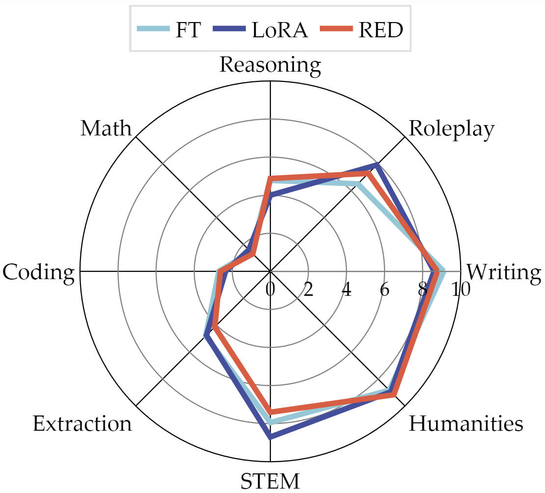
Figure 2: Scores of RED and other methods in MT-Bench. See more detailed results in Table 16 in Appendix D.

Model & Method	# Params.	BLEU	NIST	MET	ROUGE-L	CIDEr
Adapter (rank 1)	$0.25\mathbf{M}$	$63.76$	$8.37$	$42.74$	$66.70$	$2.09$
Adapter_FFN (rank 1)	$0.07\mathbf{M}$	$62.99$	$8.09$	$40.88$	$66.39$	$1.98$
LoRA (rank 1)	$0.1\mathbf{M}$	$64.51$	$8.38$	$44.78$	$67.35$	$2.28$
RED	$0.05\mathbf{M}$	$64.86$	$8.36$	$44.99$	$67.62$	$2.28$

Table 5: Comparison between RED and other rank 1 PEFT methods.

Table 4 presents the win rates on AlpacaEval of responses generated by models trained with different methods, compared to the reference responses from text-davinci-003. RED achieved a higher win rate even though the number of trainable parameters was $25,700$ times less than that of full parameter fine-tuning and $32$ times less than LoRA, indicating that the method of directly editing representations to fine-tune the model is still applicable to large-scale language models and can generate the response that humans prefer.

Moreover, Figure 2 shows the performance score achieved by these adaption methods on 1-turn questions of MT-Bench. RED’s overall performance is comparable to other baselines, and it has achieved the best results in evaluating the capabilities of Humanities and Reasoning. RED also achieved good results on six datasets of Open LLM Leaderboard, as shown in Table 18.

5 Ablation Study

In this section, we perform an ablation study to examine the impact of individual components of our method, editing representations in different positions and comparing the effectiveness of parameters between RED and other PEFT methods.

5.1 Contribution of different “edit vectors”

RED uses two different calculation types of “edit vectors”, scaling vector and bias vector, to edit representations. We remove the scaling vector and bias vector separately before editing the representation to explore the contribution of a single type of vector to this operation.

As shown in Table 6, when we remove any “edit vector” and then edit the representation, the performance on all datasets decreases to varying degrees, denoting that these two different vectors both have made contributions in the process of editing the representation. Compared to removing the scaling vector, removing the bias vector results in much more performance degradation, indicating that the bias vector plays a greater role in the process of editing representations.

Method	MRPC	CoLA	QQP
RED	$90.3$	$68.1$	$88.7$
-Scaling Vector	$89.8$	$65.9$	$87.6$
-Bias Vector	$75.8$	$46.9$	$87.2$

Table 6: Experimental results with different “edit vectors”. “-Scaling Vector” denotes that we remove the scaling vector and edit the representation by only bias vector; “-Bias Vector” denotes that we remove the bias vector and edit the representation by only scaling vector.

5.2 Position for editing representation

Houlsby et al. (2019) adds an Adapter module after both FFN and Attention sub-layers, Lin et al. (2020) only adds the Adapter module after the FFN sub-layer, and Hu et al. (2021) only adds the LoRA module in the Attention block, corresponding to different insertion positions of the PEFT component. To investigate the impact of operating different positions of the model on performance, we also designed experiments that only edited the representations after the FFN sub-layer, only edited the representations after the Attention sub-layer, and simultaneously edited the representations after the FFN and Attention sub-layer.

As shown in Table 7, editing only the representations after the FFN sub-layer yields slightly better performance compared to editing only the representations after the Attention sub-layer. Overall, there is not much change in performance compared to editing representations after both FFN and Attention sub-layer. Therefore, considering both performance and efficiency, a more favorable compromise entails restricting only editing the representations after the FFN sub-layer.

Position	MRPC	CoLA	QQP
FFN	$90.3$	$68.1$	$88.7$
Attn	$88.9$	$66.1$	$88.6$
FFN & Attn	$89.2$	$68.4$	$89.4$

Table 7: Experimental results on different positions.

5.3 Efficiency and effectiveness of parameters

When reproducing the experiments, we selected the rank of Adapter and LoRA according to the default settings of $8$ or $16$ in previous works, which may result in some parameter redundancy. Here, we set their rank to $1$ and use GPT-2 medium as the base model to conduct experiments on the E2E NLG Challenge dataset, exploring the performance comparison between RED and these PEFT methods when their parameters are most efficient.

As shown in Table 5, compared to other variants with the smallest trainable parameters for each baseline, RED still has the smallest number of trainable parameters, indicating that RED is highly parameter efficient. Moreover, RED almost surpasses these baselines, which have slightly more trainable parameters, in all metrics, proving that RED is also parameter effective.

6 Conclusion

We explore fine-tuning the model from a new perspective of directly modifying the model representation, which is different from previous works that adjusted the model weights. We propose a new PEFT method Representation EDiting (RED), which fine-tunes the model by introducing two trainable “edit vectors” to edit representations. We have conducted extensive experiments on models of different architectures and scales on various types of NLP datasets, verifying that RED can still achieve comparable or even better performance than other baselines with much fewer trainable parameters, demonstrating that RED is not only parameter efficient but also parameter effective.

Limitations

We have demonstrated the effectiveness of the new PEFT method of fine-tuning models by directly editing the representations on various NLP tasks, it would be intriguing to explore the application of this method in other modalities, such as computer vision and speech recognition. In addition, articles related to representation engineering have shown that only a very small number of examples are needed to edit the representation to control the model output. Therefore, we will also apply our method to the few-shot scenarios to explore effective PEFT methods that are both parameter-efficient and data-efficient in the future.

Appendix A Dataset And Evaluation Details

A.1 GLUE Benchmark

The GLUE benchmark, consisting of CoLA Warstadt et al. (2018), SST-2 Socher et al. (2013), MRPC Dolan and Brockett (2005), QQP Wang et al. (2018), STS-B Cer et al. (2017), MNLI Williams et al. (2017), QNLI Demszky et al. (2018) and RTE Bar-Haim et al. (2006), is used for natural language understanding.We source each dataset from Huggingface Datasets Lhoest et al. (2021) and utilize the full dataset for our experiments.

Following Ding et al. (2023) and Hu et al. (2021), we evaluate models on the validation dataset. But unlike Hu et al. (2021) which just uses the training dataset for training and the validation dataset for testing and selects the best result for each run, we have considered a more reasonable setting by dividing the validation set into validation set and test set. After each epoch training is completed, we will verify it on the validation set and record the verification results, after training all epochs, we select the model with the best performance on the validation set and test it on the test set. For datasets with a large validation set, we select 1000 samples as the validation set, and then use the remaining samples as the test set, and for datasets with a small validation set, we select half of the samples as the validation set, and then use the remaining samples as the test set, the details, and the evaluation metric are reported in Table 8.

For all experiments on RoBERTa, we run $5$ times using different random seeds and report the average results in order to ensure statistical significance. To be specific, we use $42,43,44,45,46$ these $5$ random seeds.

Dataset	#Train	#Valid	#Test	Metric
CoLA	8.5K	522	521	Mcc
SST-2	67k	436	436	Acc
MRPC	3.7K	204	204	Acc
QQP	364K	1K	39K	Acc
STS-B	5.7k	750	750	Corr
MNLI	393k	1K	8K	Acc
QNLI	105K	1K	4.5K	Acc
RTE	2.5k	139	138	Acc

Table 8: The size and evaluation metric of the split version datasets in GLUE benchmark. "Mcc", "Acc" and "Corr" represent Matthews correlation coefficient, accuracy, and Pearson correlation coefficient respectively.

A.2 E2E NLG Challenge

E2E NLG Challenge was first introduced in Novikova et al. (2017) as a dataset for training end-to-end, data-driven natural language generation systems and is commonly used for data-to-text evaluation.

We source each dataset from Huggingface Datasets and utilize the full dataset for our experiments. Specifically, this dataset contains $42.1$k training samples, $4.67$k validation samples, and $4.69$k testing samples. Following previous works, we use the official evaluation script, which reports BLEU Papineni et al. (2002), NIST Belz and Reiter (2006), METEOR Banerjee and Lavie (2005), ROUGE-L Lin (2004) and CIDEr Vedantam et al. (2014).

For all experiments on GPT-2, we run 3 times using different random seeds and report the average results in order to ensure statistical significance. To be specific, we use 42, 43, and 44 these 3 random seeds.

A.3 UltraFeedback

UltraFeedback Cui et al. (2023) consists of $64$k prompts, each of which has four LLM responses that are rated by GPT-4 according to criteria like instruction-following, honesty, and helpfulness. We construct our training dataset from UltraFeedback by selecting the highest mean score as the “chosen” response.

A.4 Open LLM Leaderboard

Open LLM Leaderboard comprises six benchmarks that cover science questions, commonsense inference, multitask accuracy, math reasoning, and truthfulness in generating answers. Specifically, it consists of ARC Mihaylov et al. (2018), HellaSwag Zellers et al. (2019), WinoGrande Sakaguchi et al. (2019), MMLU Hendrycks et al. (2020), TruthfulQA Lin et al. (2021), and GSM8K Hendrycks et al. (2021). We utilized the Eleuther AI Language Model Evaluation Harness libraryGao et al. (2023) to assess language models trained using different methods. Table 17 provides a detailed description of the leaderboard evaluation configuration and the experimental settings adopted in this study.

A.5 AlpacaEval

AlpacaEval is an automated evaluation benchmark based on LLMs. It employs GPT-4OpenAI (2023) as an annotator to compare the generated content of models over $805$ samples on simple instruction-following tasks against reference answers from text-davinci-003. Previous work has shown that using GPT-4 as an annotator correlates highly with assessments from human evaluatorsLi et al. (2023).

A.6 MT-Bench

MT-Bench Zheng et al. (2023) is a collection of challenging questions, consisting of $80$ samples, each with two turns. This benchmark also employs GPT-4 as a judge to score the responses of models. For each turn, GPT-4 will assign a score on a scale of $10$.

Appendix B Hyperparameter Used In Experiments

B.1 RoBERTA

We train using AdamW with a linear learning rate decay schedule. For a fair comparison, we restrict the model sequence length to the same for all baseline methods. Importantly, we start with the pre-trained RoBERTa large model when adapting to MRPC, RTE, and STS-B, instead of a model already adapted to MNLI. See the hyperparameters used in our experiments for Roberta-base in Table 9 and for Roberta-large in Table 10.

We evaluate after completing the training of each epoch and select the model with the best performance on the validation set for final testing. To ensure statistical significance, we run $5$ times using different random seeds and report the average results and corresponding variance for almost all these experiments.

B.2 GPT-2

We train using AdamW with a linear learning rate decay schedule. For a fair comparison, we restrict the model sequence length to the same for all baseline methods. What’s more, the Hugginface PEFT package is used when we replicate Prefix Tuning and LoRA, and the opendelta package is used when we replicate Adapter and Adapter(FFN). See the hyperparameters used in our experiments for GPT-2 medium and GPT-2 large in Table 11.

We conduct evaluation after training every $500$ train step and select the model with the best performance on the validation set for final testing. To ensure statistical significance, we run $3$ times using different random seeds and report the average results and corresponding variance for almost all these experiments.

B.3 T5

We train using AdamW with a linear learning rate decay schedule. We followed the setting of Asai et al. (2022) and conducted experiments on T5, see the hyperparameters used in our experiments for T5 base in Table 12. We conduct evaluations after completing the training of each epoch and select the model with the best performance on the validation set for final testing.

B.4 Llama-2

We train using AdamW with a cosine learning rate decay schedule. For a fair comparison, we also restrict the model sequence length to the same for all baseline methods. Table 13 displays the hyperparameters used for Llama-2.

We conduct evaluation after training every training epoch and select the model with the best performance on TruthfulQA for final testing.

For all methods, when generating different evaluation metrics, we use a greedy decoding strategy. To avoid the issue of repetition, we set the repetition penalty to $1.1$ and set the no repeat ngram size to $5$.

Appendix C Results with Standard Deviations

The standard deviation of the experiment conducted on Roberta is shown in Table 14, and the standard deviation of the experiment conducted on GPT-2 is shown in Table 15.

Appendix D Detailed Results On Llama-2

Figure 3 and Figure 4 present qualitative examples of RED compared with FT and LoRA in dialogue tasks. Table 16 presents the detailed result on MT-Bench and Table 18 presents the detailed result on open LLM.

Method & Model	Dataset	MNLI	SST-2	MRPC	CoLA	QNLI	QQP	RTE	STS-B
	Optimizer	AdamW
	LR Schedule	Linear
	Batch Size	$32$	$32$	$32$	$32$	$32$	$32$	$32$	$32$
	# Epochs	$20$	$40$	$40$	$40$	$20$	$20$	$40$	$40$
FT	Learning Rate	$1e-05$	$1e-05$	$1e-05$	$1e-05$	$1e-05$	$1e-05$	$1e-05$	$1e-05$
	Warmup Ratio	$6e-02$	$6e-02$	$6e-02$	$6e-02$	$6e-02$	$6e-02$	$6e-02$	$6e-02$
	Weight Decay	$1e-04$
	Max Seq. Len.	$256$
	Batch Size	$32$	$32$	$32$	$32$	$32$	$32$	$32$	$32$
	# Epochs	$20$	$40$	$40$	$40$	$20$	$20$	$40$	$40$
	Learning Rate	$5e-04$	$5e-04$	$4e-04$	$4e-04$	$4e-04$	$5e-04$	$5e-04$	$4e-04$
LoRA	Warmup Ratio	$6e-02$	$6e-02$	$6e-02$	$6e-02$	$6e-02$	$6e-02$	$6e-02$	$6e-02$
	LoRA Config.	$r_{q}=r_{v}=8$
	LoRA $\alpha$.	$8$
	Max Seq. Len.	$256$
	Batch Size	$32$	$32$	$32$	$32$	$32$	$32$	$32$	$32$
	# Epochs	$20$	$40$	$40$	$40$	$20$	$20$	$40$	$40$
Adapter	Learning Rate	$1e-04$	$1e-04$	$1e-04$	$1e-04$	$1e-04$	$1e-04$	$1e-04$	$1e-04$
	Warmup Ratio	$6e-02$	$6e-02$	$6e-02$	$6e-02$	$6e-02$	$6e-02$	$6e-02$	$6e-02$
	Rank.	$8$
	Max Seq. Len.	$256$
	Batch Size	$32$	$32$	$32$	$32$	$32$	$32$	$32$	$32$
	# Epochs	$20$	$40$	$40$	$40$	$20$	$20$	$40$	$40$
Adapter_FFN	Learning Rate	$1e-04$	$1e-04$	$1e-04$	$1e-04$	$1e-04$	$1e-04$	$1e-04$	$1e-04$
	Warmup Ratio	$6e-02$	$6e-02$	$6e-02$	$6e-02$	$6e-02$	$6e-02$	$6e-02$	$6e-02$
	Rank.	$16$
	Max Seq. Len.	$256$
	Batch Size	$32$	$32$	$32$	$32$	$32$	$32$	$32$	$32$
	# Epochs	$20$	$40$	$40$	$40$	$20$	$20$	$40$	$40$
BitFit	Learning Rate	$1e-04$	$1e-04$	$1e-04$	$1e-04$	$1e-04$	$1e-04$	$1e-04$	$1e-04$
	Warmup Ratio	$6e-02$	$6e-02$	$6e-02$	$6e-02$	$6e-02$	$6e-02$	$6e-02$	$6e-02$
	Max Seq. Len.	$256$
	Batch Size	$32$	$32$	$32$	$32$	$32$	$32$	$32$	$32$
	# Epochs	$20$	$40$	$40$	$40$	$20$	$20$	$40$	$40$
RED	Learning rate	$1e-03$	$1e-03$	$5e-03$	$5e-03$	$3e-03$	$1e-03$	$8e-03$	$3e-03$
	Warmup Ratio	$6e-02$	$6e-02$	$6e-02$	$6e-02$	$6e-02$	$6e-02$	$6e-02$	$6e-02$
	Max Seq. Len.	$256$

Table 9: Hyperparameters for RoBERTa based on GLUE.

Method & Model	Dataset	MNLI	SST-2	MRPC	CoLA	QNLI	QQP	RTE	STS-B
	Optimizer	AdamW
	LR Schedule	Linear
	Batch Size	$16$	$32$	$32$	$32$	$16$	$16$	$16$	$32$
	# Epochs	$10$	$10$	$20$	$20$	$10$	$10$	$20$	$10$
FT	Learning rate	$2e-05$	$2e-05$	$2e-05$	$2e-05$	$2e-05$	$1e-05$	$1e-05$	$2e-05$
	Warmup Ratio	$6e-02$	$6e-02$	$6e-02$	$6e-02$	$6e-02$	$6e-02$	$6e-02$	$6e-02$
	Weight Decay	$1e-01$
	Max Seq. Len.	$256$
	Batch Size	$32$	$32$	$32$	$32$	$32$	$32$	$32$	$32$
	# Epochs	$10$	$10$	$20$	$20$	$10$	$10$	$20$	$10$
	Learning rate	$3e-04$	$4e-04$	$3e-04$	$2e-04$	$2e-04$	$3e-04$	$4e-04$	$2e-04$
LoRA	Warmup Ratio	$6e-02$	$6e-02$	$6e-02$	$6e-02$	$6e-02$	$6e-02$	$6e-02$	$6e-02$
	LoRA Config.	$r_{q}=r_{v}=8$
	LoRA $\alpha$.	$16$
	Max Seq. Len.	$256$
	Batch Size	$32$	$32$	$32$	$32$	$32$	$32$	$32$	$32$
	# Epochs	$10$	$10$	$20$	$20$	$10$	$10$	$20$	$10$
Adapter	Learning rate	$3e-04$	$3e-04$	$3e-04$	$3e-04$	$3e-04$	$3e-04$	$3e-04$	$3e-04$
	Warmup Ratio	$6e-02$	$6e-02$	$6e-02$	$6e-02$	$6e-02$	$6e-02$	$6e-02$	$6e-02$
	Rank.	$8$
	Max Seq. Len.	$256$
	Batch Size	$32$	$32$	$32$	$32$	$32$	$32$	$32$	$32$
	# Epochs	$10$	$10$	$20$	$20$	$10$	$10$	$20$	$10$
Adapter_FFN	Learning rate	$3e-04$	$3e-04$	$3e-04$	$3e-04$	$3e-04$	$3e-04$	$3e-04$	$3e-04$
	Warmup Ratio	$6e-02$	$6e-02$	$6e-02$	$6e-02$	$6e-02$	$6e-02$	$6e-02$	$6e-02$
	Rank.	$16$
	Max Seq. Len.	$256$
	Batch Size	$32$	$32$	$32$	$32$	$32$	$32$	$32$	$32$
	# Epochs	$10$	$10$	$20$	$20$	$10$	$10$	$20$	$10$
RED	Learning rate	$1e-03$	$1e-03$	$2e-03$	$1e-03$	$1e-03$	$1e-03$	$5e-03$	$5e-03$
	Weight Decay	$0.0$	$0.0$	$0.0$	$0.0$	$0.0$	$0.0$	$1e-04$	$0.0$
	Warmup Ratio	$6e-02$	$6e-02$	$0$	$6e-02$	$6e-02$	$6e-02$	$1e-02$	$6e-02$
	Max Seq. Len.	$256$

Table 10: Hyperparameters for RoBERTa large on GLUE.

Dataset	E2E NLG Challenge
	Training
	FT	FT_top2	Adapter	Apapter_FFN	LoRA	Prefix Tuning	RED_M	RED_L
Optimizer	AdamW	AdamW	AdamW	AdamW	AdamW	AdamW	AdamW	AdamW
Weight Decay	$0.0$	$0.0$	$0.0$	$0.0$	$1e-02$	$0.0$	$1e-04$	$0.0$
# Epoch	$5$	$5$	$5$	$5$	$5$	$5$	$5$	$10$
Learning Rate Schedule	Linear	Linear	Linear	Linear	Linear	Linear	Linear	Linear
Label Smooth	$0.0$	$0.0$	$0.0$	$0.0$	$0.1$	$0.0$	$0.0$	$0.0$
Learning Rate	$5e-05$	$5e-05$	$8e-05$	$8e-05$	$2e-04$	$8e-05$	$6e-02$	$5e-05$
Rank or Prefix Length	-	-	$8$	$16$	$8$	$16$	-	-
Lora $\alpha$	-	-	-	-	$32$	-	-	-
Adaption	-	-	-	-	$r_{q}=r_{v}=r_{k}=8$	-	-	-
Warmup Steps	$500$	$500$	$500$	$500$	$500$	$500$	$500$	$500$
Batch Size	$10$	$10$	$10$	$10$	$10$	$10$	$10$	$10$
	Inference
Beam Size	$10$
Length Penalty	$0.9$
no repeat ngram size	$4$

Table 11: Hyperparameters for GPT-2 on E2E NLG Challenge. RED_M represents hyperparameters applied on GPT-2 medium and RED_L represents hyperparameters applied on GPT-2 large.

Method & Model	Dataset	MNLI	SST-2	MRPC	CoLA	QNLI	QQP	RTE	STS-B
	Optimizer	AdamW
	LR Schedule	Linear
	Batch Size	$32$	$32$	$32$	$32$	$32$	$32$	$32$	$32$
	# Epochs	$10$	$10$	$20$	$60$	$10$	$10$	$30$	$50$
RED	Learning rate	$5e-02$	$3e-02$	$1e-01$	$4e-02$	$2e-02$	$5e-03$	$7e-02$	$4e-02$
	Warmup Ratio	$1e-02$	$6e-02$	$1e-02$	$1e-02$	$0e-00$	$1e-02$	$1e-02$	$6e-02$
	Max Seq. Len.	$256$

Table 12: Hyperparameters for T5 base on GLUE.

Method	Hyperparameter	Value
	Batch Size	$128$
	Micro Batch Size	$2$
	Optimizer	Adamw
	LR Scheduler Type	Cosine
	Rarmup Ratio	$0.1$
	Max Seq. Len.	$768$
FT	Learning Rate	$2e-5$
	# Epochs	$3$
LoRA	Learning Rate	$3e-4$
	# Epochs	$3$
	Batch Size	$128$
	LoRA $\alpha$	$16$
	LoRA Dropout	$0.1$
	LoRA Rank	$16$
	Target Modules	[q_proj, v_proj]
RED	Learning Rate	$1e-3$
	# Epochs	$10$

Table 13: Hyperparameters used for Llama-2.

Model & Method	# Params.	MNLI	SST-2	MRPC	CoLA	QNLI	QQP	RTE	STS-B	Avg.
FT (base)	$125\mathbf{M}$	$87.3$	$94.4$	$87.9$	$62.4$	$92.5$	$91.7$	$78.3$	$90.6$	$85.6$
		$(0.34)$	$(0.96)$	$(0.91)$	$(3.29)$	$(0.22)$	$(0.19)$	$(3.20)$	$(0.59)$
Adapter (base)	$0.4\mathbf{M}$	$87.0$	$93.3$	$88.4$	$60.9$	$92.5$	$90.5$	$76.6$	$90.5$	$85.0$
		$(0.28)$	$(0.40)$	$(1.54)$	$(3.09)$	$(0.02)$	$(0.08)$	$(2.26)$	$(0.35)$
Adapter_FFN (base)	$0.3\mathbf{M}$	$87.1$	$93.0$	$88.8$	$58.5$	$92.1$	$90.2$	$77.7$	$90.4$	$84.7$
		$(0.10)$	$(0.50)$	$(1.38)$	$(1.69)$	$(0.28)$	$(0.07)$	$(1.93)$	$(0.31)$
LoRA (base)	$0.3\mathbf{M}$	$86.6$	$93.9$	$88.7$	$59.7$	$92.6$	$90.4$	$75.3$	$90.3$	$84.7$
		$(0.23)$	$(0.49)$	$(0.76)$	$(4.36)$	$(0.10)$	$(0.08)$	$(2.79)$	$(0.54)$
BitFit (base)	$0.1\mathbf{M}$	$84.7$	$94.0$	$88.1$	$54.0$	$91.0$	$87.3$	$69.8$	$89.5$	$82.3$
		$(0.08)$	$(0.87)$	$(1.57)$	$(3.07)$	$(0.05)$	$(0.02)$	$(1.51)$	$(0.35)$
RED (base)	$0.02\mathbf{M}$	$83.9$	$93.9$	$89.2$	$61.0$	$90.7$	$87.2$	$78.0$	$90.4$	$84.7$
		$(0.14)$	$(0.31)$	$(0.98)$	$(2.96)$	$(0.35)$	$(0.17)$	$(2.06)$	$(0.32)$
FT (large)	$355\mathbf{M}$	$88.8$	$96.0$	$91.7$	$68.2$	$93.8$	$91.5$	$85.8$	$92.6$	$88.5$
		$(0.45)$	$(0.66)$	$(1.73)$	$(2.62)$	$(0.33)$	$(1.28)$	$(1.40)$	$(0.16)$
LoRA (large)	$0.8\mathbf{M}$	$90.2$	$96.0$	$89.8$	$65.5$	$94.7$	$90.7$	$86.3$	$91.7$	$88.1$
		$(0.25)$	$(0.85)$	$(2.09)$	$(2.02)$	$(0.21)$	$(0.91)$	$(2.41)$	$(0.44)$
Adapter (large)	$0.9\mathbf{M}$	$90.1$	$95.2$	$90.5$	$65.4$	$94.6$	$91.4$	$85.3$	$91.5$	$88.0$
		$(0.12)$	$(0.48)$	$(0.59)$	$(2.24)$	$(0.17)$	$(0.13)$	$(1.34)$	$(0.33)$
Adapter_FFN (large)	$0.8\mathbf{M}$	$90.3$	$96.1$	$90.5$	$64.4$	$94.3$	$91.3$	$84.8$	$90.2$	$87.7$
		$(0.15)$	$(0.75)$	$(1.26)$	$(1.56)$	$(0.39)$	$(0.24)$	$(2.01)$	$(0.24)$
RED (large)	$0.05\mathbf{M}$	$89.5$	$96.0$	$90.3$	$68.1$	$93.5$	$88.8$	$86.2$	$91.3$	$87.9$
		$(0.38)$	$(0.48)$	$(1.40)$	$(1.69)$	$(0.33)$	$(0.11)$	$(1.40)$	$(0.21)$

Table 14: Test results of RED and other adaption methods on the GLUE benchmark. The standard deviation is provided in parentheses.

Model & Method	# Params.	BLEU	NIST	MET	ROUGE-L	CIDEr
FT (medium)	$355\mathbf{M}$	$65.95$	$8.52$	$45.95$	$69.13$	$2.35$
		$(0.26)$	$(0.03)$	$(0.07)$	$(0.30)$	$(0.01)$
$\mathbf{FT^{top2}}$ (medium)	$25.2\mathbf{M}$	$65.95$	$8.52$	$45.95$	$69.13$	$2.35$
		$(0.33)$	$(0.03)$	$(0.09)$	$(0.17)$	$(0.02)$
Adapter (medium)	$0.9\mathbf{M}$	$64.31$	$8.29$	$44.91$	$67.72$	$2.28$
		$(0.17)$	$(0.01)$	$(0.29)$	$(0.26)$	$(0.01)$
Adapter_FFN (medium)	$0.8\mathbf{M}$	$64.41$	$8.30$	$44.74$	$67.53$	$2.29$
		$(0.17)$	$(0.02)$	$(0.11)$	$(0.02)$	$(0.01)$
LoRA (medium)	$0.8\mathbf{M}$	$67.43$	$8.65$	$46.01$	$69.64$	$2.42$
		$(0.39)$	$(0.05)$	$(0.07)$	$(0.14)$	$(0.01)$
Prefix Tuning (medium)	$0.8\mathbf{M}$	$63.92$	$8.26$	$41.81$	$66.86$	$2.03$
		$(0.27)$	$(0.11)$	$(0.62)$	$(0.22)$	$(0.05)$
RED (medium)	$0.05\mathbf{M}$	$64.86$	$8.36$	$44.99$	$67.62$	$2.28$
		$(0.40)$	$(0.03)$	$(0.02)$	$(0.22)$	$(0.01)$
FT (large)	$774\mathbf{M}$	$65.56$	$8.50$	$45.40$	$68.38$	$2.27$
		$(0.47)$	$(0.05)$	$(0.29)$	$(0.23)$	$(0.02)$
Adapter (large)	$1.8\mathbf{M}$	$65.94$	$8.46$	$45.78$	$68.65$	$2.34$
		$(0.35)$	$(0.05)$	$(0.11)$	$(0.35)$	$(0.01)$
Adapter_FFN (large)	$1.5\mathbf{M}$	$65.53$	$8.41$	$45.65$	$68.46$	$2.33$
		$(0.61)$	$(0.07)$	$(0.12)$	$(0.16)$	$(0.01)$
LoRA (large)	$1.5\mathbf{M}$	$68.24$	$8.76$	$46.23$	$69.92$	$2.42$
		$(0.28)$	$(0.04)$	$(0.04)$	$(0.16)$	$(0.01)$
Prefix Tuning (large)	$1.5\mathbf{M}$	$65.50$	$8.45$	$43.97$	$67.32$	$2.23$
		$(0.63)$	$(0.05)$	$(0.21)$	$(0.38)$	$(0.02)$
RED (large)	$0.09\mathbf{M}$	$65.77$	$8.42$	$46.12$	$69.03$	$2.36$
		$(0.48)$	$(0.06)$	$(0.10)$	$(0.09)$	$(0.02)$

Table 15: Test results of RED and other adaption methods on the E2E NLG Challenge dataset. The standard deviation is provided in parentheses.

Method	Trainable Parms.	Writing	Roleplay	Reasoning	Math	Coding	Extraction	Stem	Humanities	Average
Turn-1
FT	$6739\mathbf{M}$	$9.111$	$6.500$	$4.778$	$1.444$	$2.700$	$4.800$	$7.944$	$8.833$	$5.688$
LoRA	$8.39\mathbf{M}$	$8.600$	$7.900$	$4.000$	$1.600$	$2.350$	$4.750$	$8.700$	$8.950$	$5.856$
RED	$0.26\mathbf{M}$	$8.778$	$7.278$	$4.875$	$1.300$	$2.625$	$4.125$	$7.400$	$9.167$	$5.732$
Turn-2
FT	$6739\mathbf{M}$	$1.667$	$5.938$	$2.222$	$1.700$	$2.000$	$2.111$	$3.200$	$5.300$	$3.021$
LoRA	$8.39\mathbf{M}$	$1.900$	$5.800$	$2.100$	$1.600$	$2.550$	$1.222$	$3.100$	$5.500$	$2.994$
RED	$0.26\mathbf{M}$	$1.375$	$5.500$	$2.444$	$1.444$	$2.125$	$1.750$	$3.000$	$5.875$	$2.946$
Final
FT	$6739\mathbf{M}$	$5.389$	$6.200$	$3.500$	$1.579$	$2.412$	$3.526$	$5.447$	$6.974$	$4.354$
LoRA	$8.39\mathbf{M}$	$5.250$	$6.850$	$3.050$	$1.600$	$2.450$	$3.079$	$5.900$	$7.225$	$4.434$
RED	$0.26\mathbf{M}$	$5.294$	$6.389$	$3.588$	$1.368$	$2.375$	$2.938$	$5.750$	$7.618$	$4.401$

Table 16: Results of MT-Bench.

Datasets	Arc	TruthfulQA	Winogrande	GSM8k	HellaSwag	MMLU
# few-shot	$25$	$0$	$5$	$5$	$10$	$5$
Metric	acc_norm	mc2	acc	acc	acc_norm	acc

Table 17: For each dataset used in the evaluation on the Open LLM Leaderboard, we detail the quantity of few-shot samples utilized and the specific metric employed for evaluation.

Method	# Parms.	Arc	TruthfulQA	Winogrande	GSM8k	HellaSwag	MMLU	Average
FT	$6739\mathbf{M}$	$73.34$	$47.07$	$74.03$	$16.22$	$79.95$	$46.55$	$56.19$
LoRA	$8.39\mathbf{M}$	$72.07$	$44.84$	$75.85$	$15.01$	$78.60$	$44.42$	$55.13$
RED	$0.26\mathbf{M}$	$72.04$	$47.59$	$72.85$	$11.90$	$77.86$	$42.27$	$54.09$

Table 18: Results of different methods on six benchmarks of Open LLM Leaderboard.

References

- Aghajanyan et al. (2020) Armen Aghajanyan, Luke Zettlemoyer, and Sonal Gupta. 2020. Intrinsic dimensionality explains the effectiveness of language model fine-tuning. arXiv preprint arXiv:2012.13255.
- Asai et al. (2022) Akari Asai, Mohammadreza Salehi, Matthew E. Peters, and Hannaneh Hajishirzi. 2022. Attempt: Parameter-efficient multi-task tuning via attentional mixtures of soft prompts. In Conference on Empirical Methods in Natural Language Processing.
- Banerjee and Lavie (2005) Satanjeev Banerjee and Alon Lavie. 2005. Meteor: An automatic metric for mt evaluation with improved correlation with human judgments. In IEEvaluation@ACL.
- Bar-Haim et al. (2006) Roy Bar-Haim, Ido Dagan, Bill Dolan, Lisa Ferro, Danilo Giampiccolo, Bernardo Magnini, and Idan Szpektor. 2006. The second pascal recognising textual entailment challenge.
- Beeching et al. (2023) Edward Beeching, Clémentine Fourrier, Nathan Habib, Sheon Han, Nathan Lambert, Nazneen Rajani, Omar Sanseviero, Lewis Tunstall, and Thomas Wolf. 2023. Open llm leaderboard. https://huggingface.co/spaces/HuggingFaceH4/open_llm_leaderboard.
- Belz and Reiter (2006) Anja Belz and Ehud Reiter. 2006. Comparing automatic and human evaluation of nlg systems. In Conference of the European Chapter of the Association for Computational Linguistics.
- Ben-Zaken et al. (2021) Elad Ben-Zaken, Shauli Ravfogel, and Yoav Goldberg. 2021. Bitfit: Simple parameter-efficient fine-tuning for transformer-based masked language-models. ArXiv, abs/2106.10199.
- Brown et al. (2020) Tom Brown, Benjamin Mann, Nick Ryder, Melanie Subbiah, Jared D Kaplan, Prafulla Dhariwal, Arvind Neelakantan, Pranav Shyam, Girish Sastry, Amanda Askell, et al. 2020. Language models are few-shot learners. Advances in neural information processing systems, 33:1877–1901.
- Cer et al. (2017) Daniel Matthew Cer, Mona T. Diab, Eneko Agirre, Iñigo Lopez-Gazpio, and Lucia Specia. 2017. Semeval-2017 task 1: Semantic textual similarity multilingual and crosslingual focused evaluation. In International Workshop on Semantic Evaluation.
- Cui et al. (2023) Ganqu Cui, Lifan Yuan, Ning Ding, Guanming Yao, Wei Zhu, Yuan Ni, Guotong Xie, Zhiyuan Liu, and Maosong Sun. 2023. Ultrafeedback: Boosting language models with high-quality feedback. ArXiv, abs/2310.01377.
- Demszky et al. (2018) Dorottya Demszky, Kelvin Guu, and Percy Liang. 2018. Transforming question answering datasets into natural language inference datasets. ArXiv, abs/1809.02922.
- Dettmers et al. (2023) Tim Dettmers, Artidoro Pagnoni, Ari Holtzman, and Luke Zettlemoyer. 2023. Qlora: Efficient finetuning of quantized llms. ArXiv, abs/2305.14314.
- Devlin et al. (2018) Jacob Devlin, Ming-Wei Chang, Kenton Lee, and Kristina Toutanova. 2018. Bert: Pre-training of deep bidirectional transformers for language understanding. arXiv preprint arXiv:1810.04805.
- Ding et al. (2023) Ning Ding, Xingtai Lv, Qiaosen Wang, Yulin Chen, Bowen Zhou, Zhiyuan Liu, and Maosong Sun. 2023. Sparse low-rank adaptation of pre-trained language models. arXiv preprint arXiv:2311.11696.
- Ding et al. (2022) Ning Ding, Yujia Qin, Guang Yang, Fuchao Wei, Zonghan Yang, Yusheng Su, Shengding Hu, Yulin Chen, Chi-Min Chan, Weize Chen, et al. 2022. Delta tuning: A comprehensive study of parameter efficient methods for pre-trained language models. arXiv preprint arXiv:2203.06904.
- Dolan and Brockett (2005) William B. Dolan and Chris Brockett. 2005. Automatically constructing a corpus of sentential paraphrases. In International Joint Conference on Natural Language Processing.
- Gao et al. (2023) Leo Gao, Jonathan Tow, Baber Abbasi, Stella Biderman, Sid Black, Anthony DiPofi, Charles Foster, Laurence Golding, Jeffrey Hsu, Alain Le Noac’h, Haonan Li, Kyle McDonell, Niklas Muennighoff, Chris Ociepa, Jason Phang, Laria Reynolds, Hailey Schoelkopf, Aviya Skowron, Lintang Sutawika, Eric Tang, Anish Thite, Ben Wang, Kevin Wang, and Andy Zou. 2023. A framework for few-shot language model evaluation.
- Guo et al. (2020) Demi Guo, Alexander M Rush, and Yoon Kim. 2020. Parameter-efficient transfer learning with diff pruning. arXiv preprint arXiv:2012.07463.
- He et al. (2021) Junxian He, Chunting Zhou, Xuezhe Ma, Taylor Berg-Kirkpatrick, and Graham Neubig. 2021. Towards a unified view of parameter-efficient transfer learning. ArXiv, abs/2110.04366.
- Hendrycks et al. (2020) Dan Hendrycks, Collin Burns, Steven Basart, Andy Zou, Mantas Mazeika, Dawn Xiaodong Song, and Jacob Steinhardt. 2020. Measuring massive multitask language understanding. ArXiv, abs/2009.03300.
- Hendrycks et al. (2021) Dan Hendrycks, Collin Burns, Saurav Kadavath, Akul Arora, Steven Basart, Eric Tang, Dawn Xiaodong Song, and Jacob Steinhardt. 2021. Measuring mathematical problem solving with the math dataset. ArXiv, abs/2103.03874.
- Houlsby et al. (2019) Neil Houlsby, Andrei Giurgiu, Stanislaw Jastrzebski, Bruna Morrone, Quentin De Laroussilhe, Andrea Gesmundo, Mona Attariyan, and Sylvain Gelly. 2019. Parameter-efficient transfer learning for nlp. In International Conference on Machine Learning, pages 2790–2799. PMLR.
- Hu et al. (2021) Edward J Hu, Yelong Shen, Phillip Wallis, Zeyuan Allen-Zhu, Yuanzhi Li, Shean Wang, Lu Wang, and Weizhu Chen. 2021. Lora: Low-rank adaptation of large language models. arXiv preprint arXiv:2106.09685.
- Jia et al. (2022) Menglin Jia, Luming Tang, Bor-Chun Chen, Claire Cardie, Serge Belongie, Bharath Hariharan, and Ser-Nam Lim. 2022. Visual prompt tuning. In European Conference on Computer Vision, pages 709–727. Springer.
- Karimi Mahabadi et al. (2021) Rabeeh Karimi Mahabadi, James Henderson, and Sebastian Ruder. 2021. Compacter: Efficient low-rank hypercomplex adapter layers. Advances in Neural Information Processing Systems, 34:1022–1035.
- Kopiczko et al. (2023) Dawid Jan Kopiczko, Tijmen Blankevoort, and Yuki Markus Asano. 2023. Vera: Vector-based random matrix adaptation. ArXiv, abs/2310.11454.
- Lee et al. (2019) Jaejun Lee, Raphael Tang, and Jimmy J. Lin. 2019. What would elsa do? freezing layers during transformer fine-tuning. ArXiv, abs/1911.03090.
- Lester et al. (2021a) Brian Lester, Rami Al-Rfou, and Noah Constant. 2021a. The power of scale for parameter-efficient prompt tuning. arXiv preprint arXiv:2104.08691.
- Lester et al. (2021b) Brian Lester, Rami Al-Rfou, and Noah Constant. 2021b. The power of scale for parameter-efficient prompt tuning. In Conference on Empirical Methods in Natural Language Processing.
- Lhoest et al. (2021) Quentin Lhoest, Albert Villanova del Moral, Yacine Jernite, Abhishek Thakur, Patrick von Platen, Suraj Patil, Julien Chaumond, Mariama Drame, Julien Plu, Lewis Tunstall, Joe Davison, Mario vSavsko, Gunjan Chhablani, Bhavitvya Malik, Simon Brandeis, Teven Le Scao, Victor Sanh, Canwen Xu, Nicolas Patry, Angelina McMillan-Major, Philipp Schmid, Sylvain Gugger, Clement Delangue, Th’eo Matussiere, Lysandre Debut, Stas Bekman, Pierric Cistac, Thibault Goehringer, Victor Mustar, François Lagunas, Alexander M. Rush, and Thomas Wolf. 2021. Datasets: A community library for natural language processing. ArXiv, abs/2109.02846.
- Li and Liang (2021a) Xiang Lisa Li and Percy Liang. 2021a. Prefix-tuning: Optimizing continuous prompts for generation. arXiv preprint arXiv:2101.00190.
- Li and Liang (2021b) Xiang Lisa Li and Percy Liang. 2021b. Prefix-tuning: Optimizing continuous prompts for generation. Proceedings of the 59th Annual Meeting of the Association for Computational Linguistics and the 11th International Joint Conference on Natural Language Processing (Volume 1: Long Papers), abs/2101.00190.
- Li et al. (2023) Xuechen Li, Tianyi Zhang, Yann Dubois, Rohan Taori, Ishaan Gulrajani, Carlos Guestrin, Percy Liang, and Tatsunori B Hashimoto. 2023. Alpacaeval: An automatic evaluator of instruction-following models.
- Lian et al. (2022) Dongze Lian, Daquan Zhou, Jiashi Feng, and Xinchao Wang. 2022. Scaling & shifting your features: A new baseline for efficient model tuning. ArXiv, abs/2210.08823.
- Lin (2004) Chin-Yew Lin. 2004. Rouge: A package for automatic evaluation of summaries. In Annual Meeting of the Association for Computational Linguistics.
- Lin et al. (2021) Stephanie C. Lin, Jacob Hilton, and Owain Evans. 2021. Truthfulqa: Measuring how models mimic human falsehoods. In Annual Meeting of the Association for Computational Linguistics.
- Lin et al. (2020) Zhaojiang Lin, Andrea Madotto, and Pascale Fung. 2020. Exploring versatile generative language model via parameter-efficient transfer learning. In Findings.
- Liu et al. (2022) Haokun Liu, Derek Tam, Mohammed Muqeeth, Jay Mohta, Tenghao Huang, Mohit Bansal, and Colin Raffel. 2022. Few-shot parameter-efficient fine-tuning is better and cheaper than in-context learning. ArXiv, abs/2205.05638.
- Liu et al. (2023) Wenhao Liu, Xiaohua Wang, Muling Wu, Tianlong Li, Changze Lv, Zixuan Ling, Jianhao Zhu, Cenyuan Zhang, Xiaoqing Zheng, and Xuanjing Huang. 2023. Aligning large language models with human preferences through representation engineering.
- Liu et al. (2019) Yinhan Liu, Myle Ott, Naman Goyal, Jingfei Du, Mandar Joshi, Danqi Chen, Omer Levy, Mike Lewis, Luke Zettlemoyer, and Veselin Stoyanov. 2019. Roberta: A robustly optimized bert pretraining approach. ArXiv, abs/1907.11692.
- Mao et al. (2021) Yuning Mao, Lambert Mathias, Rui Hou, Amjad Almahairi, Hao Ma, Jiawei Han, Wen tau Yih, and Madian Khabsa. 2021. Unipelt: A unified framework for parameter-efficient language model tuning. In Annual Meeting of the Association for Computational Linguistics.
- Mihaylov et al. (2018) Todor Mihaylov, Peter Clark, Tushar Khot, and Ashish Sabharwal. 2018. Can a suit of armor conduct electricity? a new dataset for open book question answering. In Conference on Empirical Methods in Natural Language Processing.
- Novikova et al. (2017) Jekaterina Novikova, Ondrej Dusek, and Verena Rieser. 2017. The e2e dataset: New challenges for end-to-end generation. ArXiv, abs/1706.09254.
- OpenAI (2023) OpenAI. 2023. GPT-4 technical report. CoRR, abs/2303.08774.
- Papineni et al. (2002) Kishore Papineni, Salim Roukos, Todd Ward, and Wei-Jing Zhu. 2002. Bleu: a method for automatic evaluation of machine translation. In Annual Meeting of the Association for Computational Linguistics.
- Pfeiffer et al. (2020) Jonas Pfeiffer, Aishwarya Kamath, Andreas Rücklé, Kyunghyun Cho, and Iryna Gurevych. 2020. Adapterfusion: Non-destructive task composition for transfer learning. ArXiv, abs/2005.00247.
- Radford et al. (2018) Alec Radford, Karthik Narasimhan, Tim Salimans, Ilya Sutskever, et al. 2018. Improving language understanding by generative pre-training.
- Radford et al. (2019) Alec Radford, Jeff Wu, Rewon Child, David Luan, Dario Amodei, and Ilya Sutskever. 2019. Language models are unsupervised multitask learners.
- Raffel et al. (2020) Colin Raffel, Noam Shazeer, Adam Roberts, Katherine Lee, Sharan Narang, Michael Matena, Yanqi Zhou, Wei Li, and Peter J Liu. 2020. Exploring the limits of transfer learning with a unified text-to-text transformer. The Journal of Machine Learning Research, 21(1):5485–5551.
- Rücklé et al. (2020) Andreas Rücklé, Gregor Geigle, Max Glockner, Tilman Beck, Jonas Pfeiffer, Nils Reimers, and Iryna Gurevych. 2020. Adapterdrop: On the efficiency of adapters in transformers. In Conference on Empirical Methods in Natural Language Processing.
- Sakaguchi et al. (2019) Keisuke Sakaguchi, Ronan Le Bras, Chandra Bhagavatula, and Yejin Choi. 2019. An adversarial winograd schema challenge at scale.
- Shin et al. (2020) Taylor Shin, Yasaman Razeghi, Robert L Logan IV, Eric Wallace, and Sameer Singh. 2020. Eliciting knowledge from language models using automatically generated prompts. ArXiv, abs/2010.15980.
- Socher et al. (2013) Richard Socher, Alex Perelygin, Jean Wu, Jason Chuang, Christopher D. Manning, A. Ng, and Christopher Potts. 2013. Recursive deep models for semantic compositionality over a sentiment treebank. In Conference on Empirical Methods in Natural Language Processing.
- Stickland and Murray (2019) Asa Cooper Stickland and Iain Murray. 2019. Bert and pals: Projected attention layers for efficient adaptation in multi-task learning. In International Conference on Machine Learning, pages 5986–5995. PMLR.
- Subramani et al. (2022) Nishant Subramani, Nivedita Suresh, and Matthew E. Peters. 2022. Extracting latent steering vectors from pretrained language models. ArXiv, abs/2205.05124.
- Touvron et al. (2023) Hugo Touvron, Louis Martin, Kevin R. Stone, Peter Albert, Amjad Almahairi, Yasmine Babaei, Nikolay Bashlykov, Soumya Batra, Prajjwal Bhargava, Shruti Bhosale, Daniel M. Bikel, Lukas Blecher, Cristian Cantón Ferrer, Moya Chen, Guillem Cucurull, David Esiobu, Jude Fernandes, Jeremy Fu, Wenyin Fu, Brian Fuller, Cynthia Gao, Vedanuj Goswami, Naman Goyal, Anthony S. Hartshorn, Saghar Hosseini, Rui Hou, Hakan Inan, Marcin Kardas, Viktor Kerkez, Madian Khabsa, Isabel M. Kloumann, A. V. Korenev, Punit Singh Koura, Marie-Anne Lachaux, Thibaut Lavril, Jenya Lee, Diana Liskovich, Yinghai Lu, Yuning Mao, Xavier Martinet, Todor Mihaylov, Pushkar Mishra, Igor Molybog, Yixin Nie, Andrew Poulton, Jeremy Reizenstein, Rashi Rungta, Kalyan Saladi, Alan Schelten, Ruan Silva, Eric Michael Smith, R. Subramanian, Xia Tan, Binh Tang, Ross Taylor, Adina Williams, Jian Xiang Kuan, Puxin Xu, Zhengxu Yan, Iliyan Zarov, Yuchen Zhang, Angela Fan, Melanie Kambadur, Sharan Narang, Aurelien Rodriguez, Robert Stojnic, Sergey Edunov, and Thomas Scialom. 2023. Llama 2: Open foundation and fine-tuned chat models. ArXiv, abs/2307.09288.
- Turner et al. (2023) Alexander Matt Turner, Lisa Thiergart, David S. Udell, Gavin Leech, Ulisse Mini, and Monte Stuart MacDiarmid. 2023. Activation addition: Steering language models without optimization. ArXiv, abs/2308.10248.
- Vaswani et al. (2017) Ashish Vaswani, Noam M. Shazeer, Niki Parmar, Jakob Uszkoreit, Llion Jones, Aidan N. Gomez, Lukasz Kaiser, and Illia Polosukhin. 2017. Attention is all you need. In Neural Information Processing Systems.
- Vedantam et al. (2014) Ramakrishna Vedantam, C. Lawrence Zitnick, and Devi Parikh. 2014. Cider: Consensus-based image description evaluation. 2015 IEEE Conference on Computer Vision and Pattern Recognition (CVPR), pages 4566–4575.
- Wang et al. (2018) Alex Wang, Amanpreet Singh, Julian Michael, Felix Hill, Omer Levy, and Samuel R. Bowman. 2018. Glue: A multi-task benchmark and analysis platform for natural language understanding. In BlackboxNLP@EMNLP.
- Wang et al. (2023) Zhen Wang, Rameswar Panda, Leonid Karlinsky, Rogério Schmidt Feris, Huan Sun, and Yoon Kim. 2023. Multitask prompt tuning enables parameter-efficient transfer learning. ArXiv, abs/2303.02861.
- Warstadt et al. (2018) Alex Warstadt, Amanpreet Singh, and Samuel R. Bowman. 2018. Neural network acceptability judgments. Transactions of the Association for Computational Linguistics, 7:625–641.
- Williams et al. (2017) Adina Williams, Nikita Nangia, and Samuel R. Bowman. 2017. A broad-coverage challenge corpus for sentence understanding through inference. In North American Chapter of the Association for Computational Linguistics.
- Wolf et al. (2019) Thomas Wolf, Lysandre Debut, Victor Sanh, Julien Chaumond, Clement Delangue, Anthony Moi, Pierric Cistac, Tim Rault, Rémi Louf, Morgan Funtowicz, and Jamie Brew. 2019. Huggingface’s transformers: State-of-the-art natural language processing. ArXiv, abs/1910.03771.
- Wu et al. (2023) Muling Wu, Wenhao Liu, Jianhan Xu, Changze Lv, Zixuan Ling, Tianlong Li, Longtao Huang, Xiaoqing Zheng, and Xuanjing Huang. 2023. Parameter efficient multi-task fine-tuning by learning to transfer token-wise prompts. In Conference on Empirical Methods in Natural Language Processing.
- Zaken et al. (2021) Elad Ben Zaken, Shauli Ravfogel, and Yoav Goldberg. 2021. Bitfit: Simple parameter-efficient fine-tuning for transformer-based masked language-models. arXiv preprint arXiv:2106.10199.
- Zellers et al. (2019) Rowan Zellers, Ari Holtzman, Yonatan Bisk, Ali Farhadi, and Yejin Choi. 2019. Hellaswag: Can a machine really finish your sentence? In Annual Meeting of the Association for Computational Linguistics.
- Zhang et al. (2023a) Qingru Zhang, Minshuo Chen, Alexander Bukharin, Pengcheng He, Yu Cheng, Weizhu Chen, and Tuo Zhao. 2023a. Adaptive budget allocation for parameter-efficient fine-tuning. arXiv preprint arXiv:2303.10512.
- Zhang et al. (2023b) Qingru Zhang, Minshuo Chen, Alexander W. Bukharin, Pengcheng He, Yu Cheng, Weizhu Chen, and Tuo Zhao. 2023b. Adaptive budget allocation for parameter-efficient fine-tuning. ArXiv, abs/2303.10512.
- Zhao et al. (2020) Mengjie Zhao, Tao Lin, Martin Jaggi, and Hinrich Schütze. 2020. Masking as an efficient alternative to finetuning for pretrained language models. In Conference on Empirical Methods in Natural Language Processing.
- Zheng et al. (2023) Lianmin Zheng, Wei-Lin Chiang, Ying Sheng, Siyuan Zhuang, Zhanghao Wu, Yonghao Zhuang, Zi Lin, Zhuohan Li, Dacheng Li, Eric P. Xing, Haotong Zhang, Joseph Gonzalez, and Ion Stoica. 2023. Judging llm-as-a-judge with mt-bench and chatbot arena. ArXiv, abs/2306.05685.
- Zou et al. (2023) Andy Zou, Long Phan, Sarah Chen, James Campbell, Phillip Guo, Richard Ren, Alexander Pan, Xuwang Yin, Mantas Mazeika, Ann-Kathrin Dombrowski, Shashwat Goel, Nathaniel Li, Michael J. Byun, Zifan Wang, Alex Mallen, Steven Basart, Sanmi Koyejo, Dawn Song, Matt Fredrikson, Zico Kolter, and Dan Hendrycks. 2023. Representation engineering: A top-down approach to ai transparency. ArXiv, abs/2310.01405.