Second-Order Fine-Tuning without Pain for LLMs:
A Hessian Informed Zeroth-Order Optimizer
Abstract
Fine-tuning large language models (LLMs) with classic first-order optimizers entails prohibitive GPU memory due to the backpropagation process. Recent works have turned to zeroth-order optimizers for fine-tuning, which save substantial memory by using two forward passes. However, these optimizers are plagued by the heterogeneity of parameter curvatures across different dimensions. In this work, we propose HiZOO, a diagonal Hessian informed zeroth-order optimizer which is the first work to leverage the diagonal Hessian to enhance zeroth-order optimizer for fine-tuning LLMs. What’s more, HiZOO avoids the expensive memory cost and only increases one forward pass per step. Extensive experiments on various models (350M66B parameters) indicate that HiZOO improves model convergence, significantly reducing training steps and effectively enhancing model accuracy. Moreover, we visualize the optimization trajectories of HiZOO on test functions, illustrating its effectiveness in handling heterogeneous curvatures. Lastly, we provide theoretical proofs of convergence for HiZOO. Code is publicly available at https://anonymous.4open.science/r/HiZOO-27F8.
1 Introduction
Fine-tuning pre-trained LLMs is necessary for specific downstream tasks and first-order optimizers are widely used, such as Adam (Kingma & Ba, 2015) and AdamW (Loshchilov & Hutter, 2019). Nevertheless, these optimizers are accompanied by substantial memory consumption, primarily due to the inherent backpropagation process. To address these limitations, MeZO (Malladi et al., 2023) proposed to utilize a memory-efficient zeroth-order optimizer to estimate the gradient with just two forward passes per step, achieving numerous memory reduction.
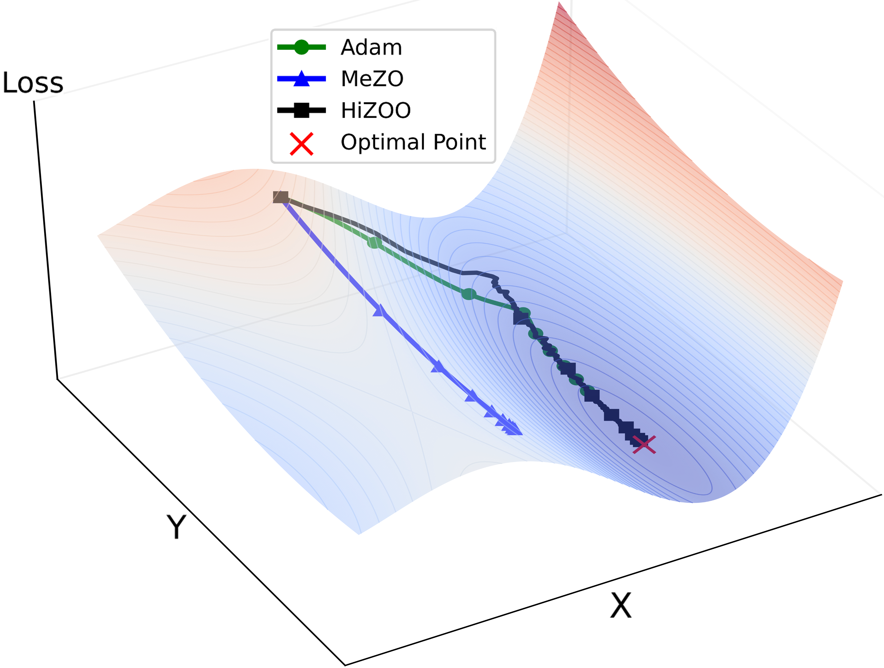
However, loss functions of LLMs often exhibit heterogeneous curvatures across different parameter dimensions, as documented in recent studies (Sagun et al., 2017; Ghorbani et al., 2019; Zhang et al., 2020). This significant difference in curvature can lead to instability or decelerated training, as shown in Figure 1. The Hessian can be leveraged in optimizer to effectively adjust the magnitude of the parameter updates (Liu & Li, 2023; Yao et al., 2021; Anil et al., 2021), solving the above dilemma. Unfortunately, in the context of zeroth-order optimization, one cannot directly compute the Hessian atop first-order derivatives.
In light of above, we propose HiZOO, leveraging the diagonal Hessian in zeroth-order optimizer to improve the convergence when training the model with heterogeneous curvatures. As shown in Figure 2, HiZOO can significantly reduce the training steps and improve the accuracy. Here we summarize our key contributions as follows:
-
1.
In HiZOO, we estimate the Hessian in zeroth-order optimization to fine-tune LLMS for the first time. Compared with classic zeroth-order optimizers, HiZOO merely increases one more forward pass per step. What’s more, HiZOO utilizes diagonal Hessian and reduces the corresponding memory cost from to .
-
2.
We provide theoretical analysis to prove that HiZOO provides an unbiased estimation of the Hessian and successfully achieve global convergence in even cases with heterogeneous curvatures across parameter dimensions.
-
3.
We conduct extensive experiments across model types (masked language models and auto-regressive language models), model scales (from 350M to 66B), and downstream tasks (classification, multiple-choice, and generation) to verify the effect of the HiZOO. Especially on SST-2 dataset, HiZOO can reduce the training time by up to 30 times (from 100k steps to 3k steps), achieving the same performance. What’s more, HiZOO finally improves the accuracy by 3% on SST-2, even better than standard full-parameter fine-tuning. When tuning OPT-66B, HiZOO reduces the model training time and performs better with up to 5% improvement and 2% improvement on average.
-
4.
We demonstrate HiZOO’s compatibility with full-parameter tuning, LoRA and prefix-tuning in Section 5. Specifically, HiZOO (prefix) outperforms MeZO (prefix) on most of the datasets and tasks across all model scales.
-
5.
Further exploration in Section 5.3 showcases that HiZOO can achieve better performance in optimizing non-differentiable objectives such as F1 score. Using the same training steps, HiZOO significantly outperforms the MeZO ’s results with 6.5% on average.
2 Related Works
Here we present a concise summary of related works on optimizers used in fine-tuning LLMs. For a more detailed review, please refer to Appendix A.
2.1 First-Order Optimizer in LLMs
First-order optimizers, such as Gradient Descent (GD), Momentum, Adagrad (Duchi et al., 2011), are fundamental in many areas like computer vision, natural languagle processing (NLP). Among them, Adam (Kingma & Ba, 2015) plays a dominant role due to its fast convergence and is often chosen for training and fine-tuning LLMs. AdamW (Loshchilov & Hutter, 2019) improves upon Adam by adding the weight decay to alleviate overfitting.
2.2 First-Order Optimizer Enhanced with Hessian
On the other hand, researchers incorporated second-order information (Hessian) to provide richer guidance for gradient descent during the training. For example BROYDEN (1970) , Nesterov & Polyak (2006) and Conn et al. (2000) utilized curvature information to pre-condition the gradient; Magoulas et al. (1999) applied diagonal Hessian as the pre-conditioner; Martens (2010) approximated the Hessian with conjugate gradient. Sophia (Liu & Li, 2023) used a light-weight estimate of the diagonal Hessian for pre-training LLMs. Despite their potential, above optimizers require the enormous GPU-memory cost.
2.3 Zeroth-Order Optimizer
Zeroth-order optimizers, with just forward passes, can greatly reduce the memory consumption. Methods like SPSA (Spall, 1992) have been shown to perform well in non-convex multi-agent optimization (Tang et al., 2021; Hajinezhad & Zavlanos, 2018) or generating black-box adversarial examples (Chen et al., 2017; Cai et al., 2021; Liu et al., 2019a; Ye et al., 2019). Recently, MeZO (Malladi et al., 2023) firstly adapted the classical ZO-SGD method to fine-tune LLMs, achieving comparable performance with significant memory reduction.
3 Methods
In the following, we briefly introduce the classical ZO gradient estimator SPSA (Spall, 1992), which is used in MeZO. Then we describe how HiZOO estimates diagonal Hessian and cooperates with zeroth-order optimizer.
3.1 Preliminaries
Definition 3.1.
(Simultaneous Perturbation Stochastic Approximation or SPSA). Given a model with parameters and loss function , SPSA estimates the gradient on a minibatch as:
where and is sampled from , is the perturbation scale. The -SPSA gradient estimate averages over randomly sampled .
3.2 Diagonal Hessian Estimator
Storing the exact full spectral Hessian () requires memory (Yao et al., 2018; Xu et al., 2019; Dembo et al., 1982), which is sufficient but never necessary. In HiZOO, we just estimate and retain only the diagonal Hessian which requires memory. It serves as a pre-conditioner to scale the direction and magnitude of the model parameter updates according to their respective curvatures.
Drawing from the lemma presented in MiNES (Ye, 2023):
| (1) |
where is the Hessian and is the approximate Hessian inverse matrix with .
Thus, we can approximate the diagonal Hessian by the zeroth order oracles. Firstly, we will access to the , and . Through the Taylor’s expansion, we yield the following results:
| (2) | ||||
Similarly, we also have:
Then we can calculate the by:
Since and are of order , we can obtain that:
Upon substituting the above results into the left side of the Eq. (1), we arrive at:
Therefore, by generalizing above equation to the multi-sampling version, we can approximate the diagonal Hessian at by:
| (3) |
where denotes the number of sampling instances for , indicating the frequency of estimation per step. A larger diminishes the variance of the diagonal Hessian estimation and simultaneously increases computational overhead. Here we adopt as the default setting and present the pseudo-code of HiZOO in Algorithm 31. Further experimental investigation into the impact of varying is available in the Section 5.7.
Above equation shows that we can approximate the diagonal entries of by , requiring just one more forward pass per step compared with MeZO.
Due to the presence of noise in the calculation of the Hessian, we utilize exponential moving average (EMA) to denoise the diagonal Hessian estimation, which commonly used in moments of gradients of Adam.
| (4) |
In the above equation, we firstly initial the and update it every step with memory cost all the time. We also use to keep all entries of to be non-negative.
3.3 Natural Gradient Estimation
Given the approximate Hessian inverse matrix , we can construct the following descent direction:
| (5) |
With the gradient descent direction, we can update as follows:
| (6) |
It’s guaranteed that can estimate the descent direction by the following equation:
| (7) | ||||
where the first and second equality are both from the Taylor’s expansion. Above equation shows that when is properly chosen, can accurately estimate the direction of gradient descent, which is the key to the success of fine-tuning large language models.
4 Convergence Analysis
| Task Type | SST-2 | SST-5 | SNLI | MNLI | RTE | TREC |
|---|---|---|---|---|---|---|
| —— sentiment —— | —— natural language inference —— | — topic — | ||||
| Zero-shot | 79.0 | 35.5 | 50.2 | 48.8 | 51.4 | 32.0 |
| LP | 76.0 (2.8) | 40.3 (1.9) | 66.0 (2.7) | 56.5 (2.5) | 59.4 (5.3) | 51.3 (5.5) |
| FT | 91.9 (1.8) | 47.5 (1.9) | 77.5 (2.6) | 70.0 (2.3) | 66.4 (7.2) | 85.0 (2.5) |
| FT (LoRA) | 91.4 (1.7) | 46.7 (1.1) | 74.9 (4.3) | 67.7 (1.4) | 66.1 (3.5) | 82.7 (4.1) |
| FT (prefix) | 91.9 (1.0) | 47.7 (1.1) | 77.2 (1.3) | 66.5 (2.5) | 66.6 (2.0) | 85.7 (1.3) |
| MeZO | 90.5 (1.2) | 45.5 (2.0) | 68.5 (3.9) | 58.7 (2.5) | 64.0 (3.3) | 76.9 (2.7) |
| MeZO (LoRA) | 91.4 (0.9) | 43.0 (1.6) | 69.7 (6.0) | 64.0 (2.5) | 64.9 (3.6) | 73.1 (6.5) |
| MeZO (prefix) | 90.8 (1.7) | 45.8 (2.0) | 71.6 (2.5) | 63.4 (1.8) | 65.4 (3.9) | 80.3 (3.6) |
| HiZOO | 93.2 (0.8) | 46.2 (1.1) | 74.6 (1.3) | 64.9 (1.7) | 66.8 ( 1.2) | 79.8 (1.3) |
| HiZOO(LoRA) | 91.2 (0.4) | 42.9 (0.8) | 71.1 (1.1) | 62.1 (1.7) | 61.4 (2.2) | 52.2 (3.2) |
| HiZOO(prefix) | 92.3 (1.2) | 47.2 (1.1) | 68.8 (1.7) | 61.6 (1.2) | 65.4 (1.2) | 82.0 (2.0) |
In Section 3, we have briefly discussed that can estimate the gradient descent direction. In this section, we will analyse that our HiZOO will converge to a stationary point. Firstly, our convergence analysis requires the following assumptions:
Assumption 4.1.
The objective function is -smooth, which means that for any , it holds that:
| (8) |
Assumption 4.2.
The stochastic gradient has variance, which means:
| (9) |
Assumption 4.3.
Each entry of lies in the range with .
Based on the above assumption of non-convex optimization, we can get the following convergence analysis.
Theorem 4.4.
Let the approximate gradient defined as:
| (10) |
Based on Assumption 4.1-4.3, we can draw the following corollary. If the update rule for is for a single step, then it’s established that:
| (11) | ||||
Furthermore, given iteration number , we choose the step size and take with uniformly sampled from . Then, we have
| (12) |
where minimizes the function . The above equation shows that as , HiZOO can converge to the optimum point.
Proof.
Detailed proof can be found in Appendix B. ∎
5 Experiments
Large language models are generally classified into two types: (1) Encoder-Decoder, also known as masked language models, such as BERT (Devlin et al., 2019) and ALBERT (Lan et al., 2020); (2) Decoder-Only, also recognized as generative language models, such as GPT family (Brown et al., 2020), OPT (Zhang et al., 2022a), LLaMA (Touvron et al., 2023).
| Task | SST-2 | RTE | CB | BoolQ | WSC | WIC | MultiRC | COPA | ReCoRD | SQuAD |
|---|---|---|---|---|---|---|---|---|---|---|
| Task type | ———————— classification ———————— | — multiple choice — | generation | |||||||
| Zero-shot | 58.8 | 59.6 | 46.4 | 59.0 | 38.5 | 55.0 | 46.9 | 80.0 | 81.2 | 46.2 |
| ICL | 87.0 | 62.1 | 57.1 | 66.9 | 39.4 | 50.5 | 53.1 | 87.0 | 82.5 | 75.9 |
| LP | 93.4 | 68.6 | 67.9 | 59.3 | 63.5 | 60.2 | 63.5 | 55.0 | 27.1 | 3.7 |
| FT (6x memory) | 92.0 | 70.8 | 83.9 | 77.1 | 63.5 | 70.1 | 71.1 | 79.0 | 74.1 | 84.9 |
| MeZO | 91.4 | 66.1 | 67.9 | 67.6 | 63.5 | 61.1 | 60.1 | 88.0 | 81.7 | 84.7 |
| MeZO(LoRA) | 89.6 | 67.9 | 66.1 | 73.8 | 64.4 | 59.7 | 61.5 | 84.0 | 81.4 | 83.8 |
| MeZO(prefix) | 90.7 | 70.8 | 69.6 | 73.1 | 57.7 | 59.9 | 63.7 | 87.0 | 81.2 | 84.2 |
| HiZOO | 91.3 | 69.3 | 69.4 | 67.3 | 63.5 | 59.4 | 55.5 | 88.0 | 81.4 | 81.9 |
| HiZOO(LoRA) | 90.59 | 67.5 | 69.6 | 70.5 | 63.5 | 60.2 | 60.2 | 87.0 | 81.9 | 83.8 |
| HiZOO(prefix) | 92.0 | 71.8 | 69.6 | 73.9 | 60.6 | 60.0 | 64.8 | 87.0 | 81.2 | 83.2 |
To rigorously assess the universality and robustness of our HiZOO, we have chosen models from each category for empirical testing. Additionally, we investigate full-parameter tuning and PEFT methods, which encompasses methods such as Low-Rank Adaptation (LoRA) (Hu et al., 2022) and prefix-tuning (Li & Liang, 2021). Detailed methodologies are presented in Appendix D.2.
5.1 Masked Language Models
Firstly, we conduct experiments on RoBERTa-large 350M (Liu et al., 2019b) on three NLP task paradigms: sentence classification, multiple choice and text generation. We follow the experimental setting (Malladi et al., 2023) in studying the few-shot and many-shot, sampling examples per class for (results in Table 1) and (results in Appendix D.2), which can reach the following observations and summaries.
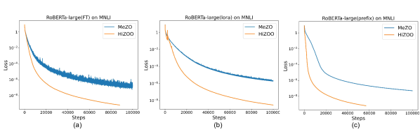
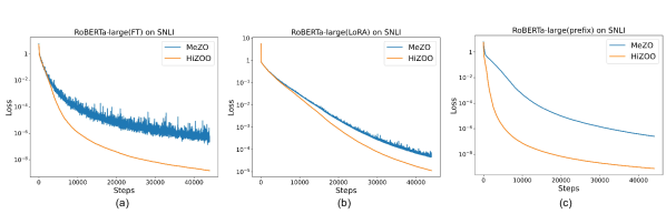
HiZOO greatly increases the convergence speed across full-parameter tuning, LoRA and prefix. As shown in Figure 3, HiZOO achieves 5× speedup over MeZO on average while getting the same training loss compared with MeZO. What’s more, the acceleration effect is stable across three tuning methods. More figures for curves of training loss are shown in Appendix D.2.
HiZOO achieves better performance compared with MeZO. Table 1 shows that HiZOO outperforms MeZO’s results with 3.56% on average on all datasets across sentiment, natural language inference and topic tasks. Specifically, HiZOO outperforms MeZO with more than 6% on SNLI and MNLI dataset.
| Task | SST-2 | RTE | BoolQ | WSC | WIC |
|---|---|---|---|---|---|
| 30B zero-shot | 56.7 | 52.0 | 39.1 | 38.5 | 50.2 |
| 30B ICL | 81.9 | 66.8 | 66.2 | 56.7 | 51.3 |
| 30B MeZO | 90.6 | 66.4 | 67.2 | 63.5 | 56.3 |
| 30B MeZO(prefix) | 87.5 | 72.6 | 73.5 | 55.8 | 59.1 |
| 30B HiZOO | 90.3 | 69.3 | 70.8 | 63.5 | 53.4 |
| 30B HiZOO(prefix) | 91.2 | 68.6 | 73.1 | 57.7 | 60.2 |
| 66B zero-shot | 57.5 | 67.2 | 66.8 | 43.3 | 50.6 |
| 66B ICL | 89.3 | 65.3 | 62.8 | 52.9 | 54.9 |
| 66B MeZO(prefix) | 93.6 | 66.4 | 73.7 | 57.7 | 58.6 |
| 66B HiZOO(prefix) | 93.6 | 71.5 | 73.2 | 60.6 | 61.1 |
5.2 Auto-Regressive Language Models
Then we extend experiments with OPT family on the same NLP task paradigms. The main results on OPT-13B are presented in Table 2. We can see that HiZOO achieves comparable (within 1%) or better performance than MeZO on all datasets. What’s more, HiZOO works well on both full-parameter tuning and PEFT methods.
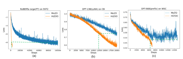
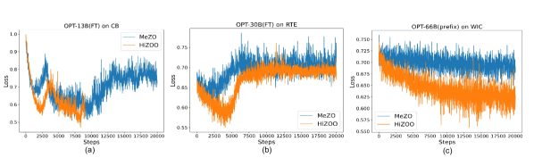
HiZOO is capable of scaling to large models with up to 66B parameters, while preserving its exceptional performance. As depicted in Table 3, on OPT-66B HiZOO (prefix) outperforms MeZO(prefix) with up to 5% increase and 2% increase on average. Figure 4 shows that at such scales HiZOO can still effectively accelerate the process for convergence and reduce the training steps.
5.3 Training with Non-Differentiable Objectives
Our proposed HiZOO employs gradient estimation to update parameters, allowing for the use of non-differentiable objectives for training. Following the setting of MeZO (Malladi et al., 2023), we conducted extensive experiments using F1 as objectives. The results presented in Table 4 indicate that our method outperforms MeZO by 6.36% on F1 on average. It’s worth noting that on TREC the improvement is even more significant (over 20%) and the original inability to converge using MeZO is solved.
| Model | RoBERTa-large (350M) | OPT-13B | |||
|---|---|---|---|---|---|
| Task | SST-2 | SST-5 | SNLI | TREC | SQuAD |
| Zero-shot | 79.0 | 35.5 | 50.2 | 32.0 | 46.2 |
| MeZO | 92.7 | 48.9 | 82.7 | 68.6 | 78.5 |
| HiZOO | 94.9 | 52.9 | 83.1 | 90 | 83.21 |
5.4 Memory Usage and Training Time Analysis
As the storage of the Hessian information, HiZOO increases a little memory usage compared to MeZO, but it still holds great advantages over FT or FT (prefix) (refer to Appendix F for detailed numbers). Specifically, using the same GPUs, HiZOO allows for tuning a model that is 5 times larger than what is feasible with FT on average, as shown in Table 5.
We also compare the training time efficiency between our HiZOO and MeZO. As we know, HiZOO requires 3 forward passes while MeZO requires 2 forward passes. Take fine-tuning RoBERTa-large as an example, although HiZOO requires the time of MeZO per step, HiZOO requires the training steps of MeZO. As a result, HiZOO can significantly reduce the overall training time by 70%. What’s more, HiZOO may converge with the smaller loss than MeZO and achieve a higher accuracy in many cases.
| Hardware | Largest OPT that can fit | |||
|---|---|---|---|---|
| FT | FT-prefix | MeZO | HiZOO | |
| 1A100 (80GB) | 2.7B | 6.7B | 30B | 13B |
| 2A100 (160GB) | 6.7B | 13B | 66B | 30B |
| 4A100 (320GB) | 13B | 30B | 66B | 66B |
| 8A100 (640GB) | 30B | 66B | 175B | 175B |
5.5 Influence of Smooth Scale
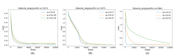
To assess the robustness of the optimizer, a grid search is conducted to evaluate the sensitivity of hyper-parameter on RoBERTa-large (350M). Figure 5 illustrates that the smoothing scale is instrumental in controlling the convergence rate during the training. As is incrementally increased from zero, the training loss decreases faster. However, excessively large values of may impede convergence or even make training fail due to overflow or gradient explosion. The experimental results indicate that yields better performance in most cases.
5.6 Trajectory Visualization on Test Functions
In this section, we evaluate the performance of the Adam, MeZO, and our HiZOO on 3 test functions with heterogeneous curvatures across different parameters:
- •
-
•
Function (b):
-
•
Function (c):
The 2D trajectories in training are illustrated in Figure 6. HiZOO and Adam are both capable of achieving convergence on Functions (a), (b), and (c), yet HiZOO consistently converges more quickly than Adam. MeZO faces challenges, only achieving effective convergence in either the or dimension, but not both, indicating a limitation in handling functions with heterogeneous curvatures. Particularly, Function (c) with its high condition number, showcases HiZOO’s remarkable ability to quickly navigate towards convergence, outperforming other methods in efficiently dealing with heterogeneous curvatures between parameter dimensions.

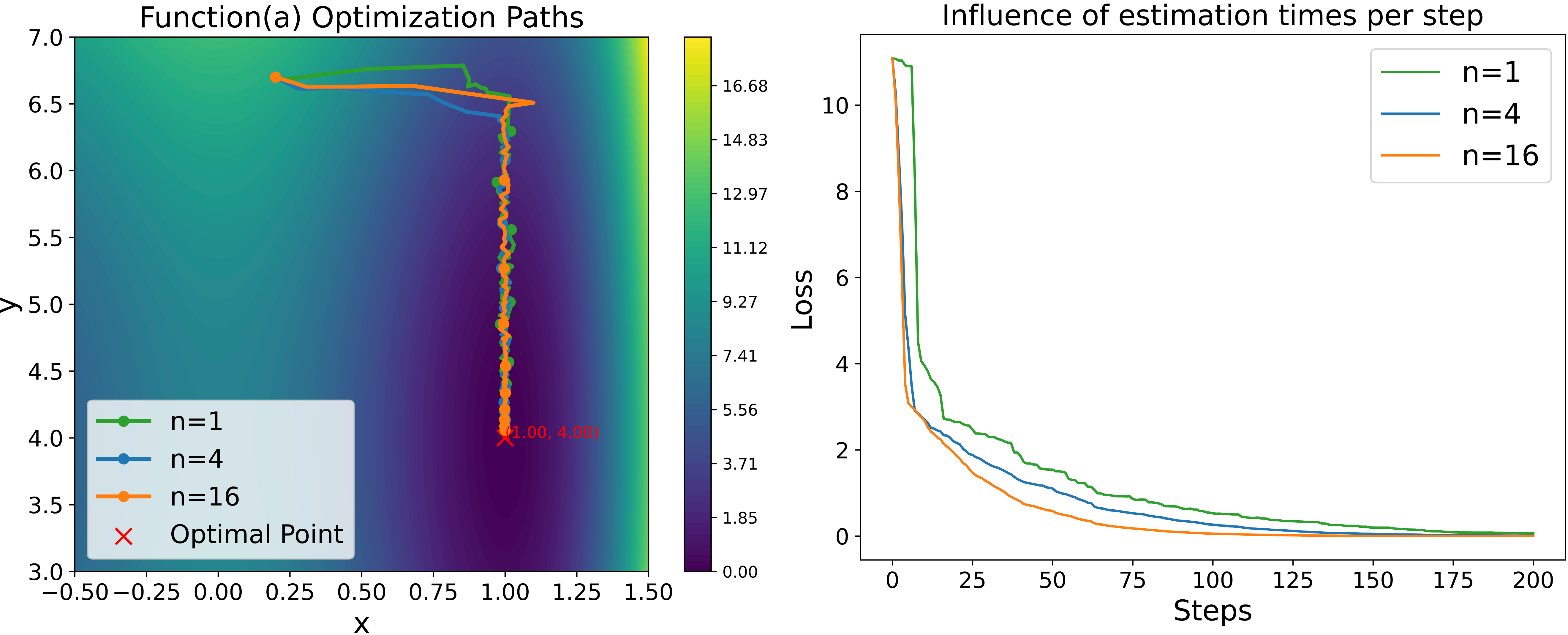
5.7 Influence of Estimation Times Per Step
Here we conduct experiments on Function (c) to explore the influence of estimation times per step. As shown in Figure 7, the bigger will decrease the variance of the diagonal Hessian estimation per step and reduces the overall training steps, but it will cause much more computation per step at the same time.
6 Conclusion
In this work, we introduced HiZOO optimizer, a diagonal Hessian enhanced zeroth-order optimizer for fine-tuning large language models across many tasks and scales. To our knowledge, HiZOO is the first ZO-SGD optimizer that incorporates diagonal Hessian for fine-tuning LLMs. Further experiment shows that HiZOO converges in much fewer steps than MeZO and achieves better performance, including LoRA, prefix and full-parameter tuning. We also conduct visualization experiments on popular test functions to show that HiZOO performs better than MeZO and comparably with Adam.
Impact Statements
This paper presents work whose goal is to advance the field of Machine Learning. There are many potential societal consequences of our work, none which we feel must be specifically highlighted here.
References
- Agarwal et al. (2009) Agarwal, A., Wainwright, M. J., Bartlett, P., and Ravikumar, P. Information-theoretic lower bounds on the oracle complexity of convex optimization. Advances in Neural Information Processing Systems, 22, 2009.
- Anil et al. (2021) Anil, R., Gupta, V., Koren, T., Regan, K., and Singer, Y. Scalable second order optimization for deep learning, 2021.
- Brown et al. (2020) Brown, T. B., Mann, B., Ryder, N., Subbiah, M., Kaplan, J., Dhariwal, P., Neelakantan, A., Shyam, P., Sastry, G., Askell, A., Agarwal, S., Herbert-Voss, A., Krueger, G., Henighan, T., Child, R., Ramesh, A., Ziegler, D. M., Wu, J., Winter, C., Hesse, C., Chen, M., Sigler, E., Litwin, M., Gray, S., Chess, B., Clark, J., Berner, C., McCandlish, S., Radford, A., Sutskever, I., and Amodei, D. Language models are few-shot learners, 2020.
- BROYDEN (1970) BROYDEN, C. G. The Convergence of a Class of Double-rank Minimization Algorithms 1. General Considerations. IMA Journal of Applied Mathematics, 6(1):76–90, 03 1970. ISSN 0272-4960. doi: 10.1093/imamat/6.1.76. URL https://doi.org/10.1093/imamat/6.1.76.
- Cai et al. (2021) Cai, H., Lou, Y., Mckenzie, D., and Yin, W. A zeroth-order block coordinate descent algorithm for huge-scale black-box optimization. In Meila, M. and Zhang, T. (eds.), Proceedings of the 38th International Conference on Machine Learning, volume 139 of Proceedings of Machine Learning Research, pp. 1193–1203. PMLR, 18–24 Jul 2021.
- Chen et al. (2017) Chen, P.-Y., Zhang, H., Sharma, Y., Yi, J., and Hsieh, C.-J. Zoo: Zeroth order optimization based black-box attacks to deep neural networks without training substitute models. New York, NY, USA, 2017. Association for Computing Machinery. ISBN 9781450352024. doi: 10.1145/3128572.3140448. URL https://doi.org/10.1145/3128572.3140448.
- Conn et al. (2000) Conn, A. R., Gould, N. I. M., and Toint, P. L. Trust-Region Methods. Society for Industrial and Applied Mathematics, USA, 2000. ISBN 0898714605.
- Dembo et al. (1982) Dembo, R. S., Eisenstat, S. C., and Steihaug, T. Inexact newton methods. SIAM Journal on Numerical Analysis, 19(2):400–408, 1982. doi: 10.1137/0719025. URL https://doi.org/10.1137/0719025.
- Devlin et al. (2019) Devlin, J., Chang, M.-W., Lee, K., and Toutanova, K. Bert: Pre-training of deep bidirectional transformers for language understanding. In North American Chapter of the Association for Computational Linguistics, 2019. URL https://api.semanticscholar.org/CorpusID:52967399.
- Duchi et al. (2011) Duchi, J., Hazan, E., and Singer, Y. Adaptive subgradient methods for online learning and stochastic optimization. J. Mach. Learn. Res., 12(null):2121–2159, jul 2011. ISSN 1532-4435.
- FairScale authors (2021) FairScale authors. Fairscale: A general purpose modular pytorch library for high performance and large scale training. https://github.com/facebookresearch/fairscale, 2021.
- George et al. (2018) George, T., Laurent, C., Bouthillier, X., Ballas, N., and Vincent, P. Fast approximate natural gradient descent in a kronecker-factored eigenbasis. In Proceedings of the 32nd International Conference on Neural Information Processing Systems, NIPS’18, pp. 9573–9583, Red Hook, NY, USA, 2018. Curran Associates Inc.
- Ghadimi & Lan (2013) Ghadimi, S. and Lan, G. Stochastic first-and zeroth-order methods for nonconvex stochastic programming. SIAM Journal on Optimization, 23(4):2341–2368, 2013.
- Ghorbani et al. (2019) Ghorbani, B., Krishnan, S., and Xiao, Y. An investigation into neural net optimization via hessian eigenvalue density. In Chaudhuri, K. and Salakhutdinov, R. (eds.), Proceedings of the 36th International Conference on Machine Learning, volume 97 of Proceedings of Machine Learning Research, pp. 2232–2241. PMLR, 09–15 Jun 2019. URL https://proceedings.mlr.press/v97/ghorbani19b.html.
- Hajinezhad & Zavlanos (2018) Hajinezhad, D. and Zavlanos, M. M. Gradient-free multi-agent nonconvex nonsmooth optimization. 2018 IEEE Conference on Decision and Control (CDC), pp. 4939–4944, 2018. URL https://api.semanticscholar.org/CorpusID:58669445.
- Hu et al. (2022) Hu, E. J., yelong shen, Wallis, P., Allen-Zhu, Z., Li, Y., Wang, S., Wang, L., and Chen, W. LoRA: Low-rank adaptation of large language models. In International Conference on Learning Representations, 2022. URL https://openreview.net/forum?id=nZeVKeeFYf9.
- Jamieson et al. (2012) Jamieson, K. G., Nowak, R., and Recht, B. Query complexity of derivative-free optimization. Advances in Neural Information Processing Systems, 25, 2012.
- Jiang et al. (2023) Jiang, S., Chen, Q., Pan, Y., Xiang, Y., Lin, Y., Wu, X., Liu, C., and Song, X. Zo-adamu optimizer: Adapting perturbation by the momentum and uncertainty in zeroth-order optimization, 2023.
- Kingma & Ba (2015) Kingma, D. and Ba, J. Adam: A method for stochastic optimization. In International Conference on Learning Representations (ICLR), San Diega, CA, USA, 2015.
- Lan et al. (2020) Lan, Z., Chen, M., Goodman, S., Gimpel, K., Sharma, P., and Soricut, R. Albert: A lite bert for self-supervised learning of language representations. In International Conference on Learning Representations, 2020. URL https://openreview.net/forum?id=H1eA7AEtvS.
- Li & Liang (2021) Li, X. L. and Liang, P. Prefix-tuning: Optimizing continuous prompts for generation. In Zong, C., Xia, F., Li, W., and Navigli, R. (eds.), Proceedings of the 59th Annual Meeting of the Association for Computational Linguistics and the 11th International Joint Conference on Natural Language Processing (Volume 1: Long Papers), pp. 4582–4597, Online, August 2021. Association for Computational Linguistics. doi: 10.18653/v1/2021.acl-long.353. URL https://aclanthology.org/2021.acl-long.353.
- Liu & Li (2023) Liu, H. and Li, Z. Sophia: A scalable stochastic second-order optimizer for language model pre-training. https://synthical.com/article/17aca766-2012-4c7c-a0f4-5b785dadabf9, 4 2023.
- Liu et al. (2019a) Liu, S., Chen, P.-Y., Chen, X., and Hong, M. signsgd via zeroth-order oracle. In International Conference on Learning Representations, 2019a. URL https://api.semanticscholar.org/CorpusID:108298677.
- Liu et al. (2019b) Liu, Y., Ott, M., Goyal, N., Du, J., Joshi, M., Chen, D., Levy, O., Lewis, M., Zettlemoyer, L., and Stoyanov, V. Roberta: A robustly optimized bert pretraining approach. arXiv preprint arXiv:1907.11692, 2019b.
- Loshchilov & Hutter (2019) Loshchilov, I. and Hutter, F. Decoupled weight decay regularization. In International Conference on Learning Representations, 2019. URL https://openreview.net/forum?id=Bkg6RiCqY7.
- Magnus et al. (1978) Magnus, J. R. et al. The moments of products of quadratic forms in normal variables. Univ., Instituut voor Actuariaat en Econometrie, 1978.
- Magoulas et al. (1999) Magoulas, G. D., Vrahatis, M. N., and Androulakis, G. S. Improving the convergence of the backpropagation algorithm using learning rate adaptation methods. Neural Comput., 11(7):1769–1796, oct 1999. ISSN 0899-7667. doi: 10.1162/089976699300016223. URL https://doi.org/10.1162/089976699300016223.
- Malladi et al. (2023) Malladi, S., Gao, T., Nichani, E., Damian, A., Lee, J. D., Chen, D., and Arora, S. Fine-tuning language models with just forward passes. In Thirty-seventh Conference on Neural Information Processing Systems, 2023. URL https://openreview.net/forum?id=Vota6rFhBQ.
- Martens (2010) Martens, J. Deep learning via hessian-free optimization. In Proceedings of the 27th International Conference on International Conference on Machine Learning, ICML’10, pp. 735–742, Madison, WI, USA, 2010. Omnipress. ISBN 9781605589077.
- Nesterov & Polyak (2006) Nesterov, Y. and Polyak, B. T. Cubic regularization of newton method and its global performance. Math. Program., 108(1):177–205, aug 2006. ISSN 0025-5610.
- Pascanu & Bengio (2014) Pascanu, R. and Bengio, Y. Revisiting natural gradient for deep networks, 2014.
- Raginsky & Rakhlin (2011) Raginsky, M. and Rakhlin, A. Information-based complexity, feedback and dynamics in convex programming. IEEE Transactions on Information Theory, 57(10):7036–7056, 2011.
- Sagun et al. (2017) Sagun, L., Bottou, L., and LeCun, Y. Eigenvalues of the hessian in deep learning: Singularity and beyond, 2017. URL https://openreview.net/forum?id=B186cP9gx.
- Schaul et al. (2013) Schaul, T., Zhang, S., and LeCun, Y. No more pesky learning rates. In Dasgupta, S. and McAllester, D. (eds.), Proceedings of the 30th International Conference on Machine Learning, volume 28 of Proceedings of Machine Learning Research, pp. 343–351, Atlanta, Georgia, USA, 17–19 Jun 2013. PMLR. URL https://proceedings.mlr.press/v28/schaul13.html.
- Spall (1992) Spall, J. Multivariate stochastic approximation using a simultaneous perturbation gradient approximation. IEEE Transactions on Automatic Control, 37(3):332–341, 1992. doi: 10.1109/9.119632.
- Spall (1997) Spall, J. C. A one-measurement form of simultaneous perturbation stochastic approximation. Automatica, 33(1):109–112, jan 1997. ISSN 0005-1098. doi: 10.1016/S0005-1098(96)00149-5. URL https://doi.org/10.1016/S0005-1098(96)00149-5.
- Tang et al. (2021) Tang, Y., Zhang, J., and Li, N. Distributed zero-order algorithms for nonconvex multiagent optimization. IEEE Transactions on Control of Network Systems, 8(1):269–281, 2021. doi: 10.1109/TCNS.2020.3024321.
- Touvron et al. (2023) Touvron, H., Lavril, T., Izacard, G., Martinet, X., Lachaux, M.-A., Lacroix, T., Rozière, B., Goyal, N., Hambro, E., Azhar, F., Rodriguez, A., Joulin, A., Grave, E., and Lample, G. Llama: Open and efficient foundation language models. ArXiv, abs/2302.13971, 2023. URL https://api.semanticscholar.org/CorpusID:257219404.
- Vakhitov et al. (2009) Vakhitov, A. T., Granichin, O. N., and Gurevich, L. S. Algorithm for stochastic approximation with trial input perturbation in the nonstationary problem of optimization. Autom. Remote Control, 70(11):1827–1835, nov 2009. ISSN 0005-1179. doi: 10.1134/S000511790911006X. URL https://doi.org/10.1134/S000511790911006X.
- Wang et al. (2020) Wang, Z., Balasubramanian, K., Ma, S., and Razaviyayn, M. Zeroth-order algorithms for nonconvex minimax problems with improved complexities. arXiv preprint arXiv:2001.07819, 2020.
- Xu et al. (2019) Xu, P., Roosta, F., and Mahoney, M. W. Newton-type methods for non-convex optimization under inexact hessian information, 2019.
- Yao et al. (2018) Yao, Z., Xu, P., Roosta-Khorasani, F., and Mahoney, M. W. Inexact non-convex newton-type methods, 2018.
- Yao et al. (2021) Yao, Z., Gholami, A., Shen, S., Mustafa, M., Keutzer, K., and Mahoney, M. Adahessian: An adaptive second order optimizer for machine learning. Proceedings of the AAAI Conference on Artificial Intelligence, 35(12):10665–10673, May 2021. doi: 10.1609/aaai.v35i12.17275. URL https://ojs.aaai.org/index.php/AAAI/article/view/17275.
- Ye (2023) Ye, H. Mirror natural evolution strategies, 2023.
- Ye et al. (2019) Ye, H., Huang, Z., Fang, C., Li, C. J., and Zhang, T. Hessian-aware zeroth-order optimization for black-box adversarial attack, 2019.
- You et al. (2020) You, Y., Li, J., Reddi, S., Hseu, J., Kumar, S., Bhojanapalli, S., Song, X., Demmel, J., Keutzer, K., and Hsieh, C.-J. Large batch optimization for deep learning: Training bert in 76 minutes. In International Conference on Learning Representations, 2020. URL https://openreview.net/forum?id=Syx4wnEtvH.
- Zeiler (2012) Zeiler, M. D. Adadelta: An adaptive learning rate method, 2012.
- Zhang et al. (2020) Zhang, J., Karimireddy, S. P., Veit, A., Kim, S., Reddi, S., Kumar, S., and Sra, S. Why are adaptive methods good for attention models? In Larochelle, H., Ranzato, M., Hadsell, R., Balcan, M., and Lin, H. (eds.), Advances in Neural Information Processing Systems, volume 33, pp. 15383–15393. Curran Associates, Inc., 2020. URL https://proceedings.neurips.cc/paper_files/paper/2020/file/b05b57f6add810d3b7490866d74c0053-Paper.pdf.
- Zhang et al. (2023) Zhang, L., Shi, S., and Li, B. Eva: Practical second-order optimization with kronecker-vectorized approximation. In The Eleventh International Conference on Learning Representations, 2023. URL https://openreview.net/forum?id=_Mic8V96Voy.
- Zhang et al. (2022a) Zhang, S., Roller, S., Goyal, N., Artetxe, M., Chen, M., Chen, S., Dewan, C., Diab, M., Li, X., Lin, X. V., Mihaylov, T., Ott, M., Shleifer, S., Shuster, K., Simig, D., Koura, P. S., Sridhar, A., Wang, T., and Zettlemoyer, L. Opt: Open pre-trained transformer language models, 2022a.
- Zhang et al. (2022b) Zhang, Y., Zhou, Y., Ji, K., and Zavlanos, M. M. A new one-point residual-feedback oracle for black-box learning and control. Automatica, 136(C), feb 2022b. ISSN 0005-1098. doi: 10.1016/j.automatica.2021.110006. URL https://doi.org/10.1016/j.automatica.2021.110006.
Appendix A Related Works
A.1 First-order Optimizer Used in LLMs
Optimization methods have consistently been a popular research domain, encompassing techniques such as Gradient Descent (GD), Momentum, Adagrad (Duchi et al., 2011), ADADELTA (Zeiler, 2012), and Newton’s method, which have been instrumental in advancing fields like computer vision. However, the emergence of large-scale models, characterized by their massive parameter counts and intricate architectures, has challenged the efficacy of conventional optimization methods for training tasks. Amidst this landscape, Adam (Kingma & Ba, 2015) has emerged as the preferred choice for its ability to rapidly converge, making it particularly suitable for the training and fine-tuning large models. Then AdamW (Loshchilov & Hutter, 2019) was proposed to add a weight decay coefficient to alleviate over-fitting. Notwithstanding these advancements, a limitation persists with these optimizers: they have an implicit batch size ceiling. Exceeding this threshold can provoke extreme gradient updates, thus impeding the convergence rate of the models. This bottleneck is particularly problematic in the context of large-model training, which typically necessitates substantial batch sizes. To circumvent this constraint, LAMB (You et al., 2020) was devised to apply principled layer-wise adaptation strategy to accelerate the training of large models employing large batches.
A.2 Hessian Based First-Order Optimizer
Compared with first-order optimizers, second-order optimizer considers second-order information in the process of gradient calculation. As a result, it has more abundant information to guide gradient descent and is considered to be more promising. Previous studies utilized curvature information to pre-condition the gradient (BROYDEN, 1970; Nesterov & Polyak, 2006; Conn et al., 2000). Subsequently, Magoulas et al. (1999) applied diagonal Hessian as the pre-conditioner, which greatly promotes the landing of second-order optimizer in the field of deep learning. Martens (2010) approximated the Hessian with conjugate gradient. Schaul et al. (2013) utilized diagonal Hessian to automatically adjust the learning rate of SGD during training. Pascanu & Bengio (2014) extended natural gradient descent to incorporate second order information alongside the manifold information and used a truncated Newton approach for inverting the metric matrix instead of using a diagonal approximation of it. EVA (Zhang et al., 2023) proposed to use the Kronecker factorization of two small vectors to approximated the Hessian, which significantly reduces memory consumption. AdaHessian (Yao et al., 2021) incorporates an approximate Hessian diagonal, with spatial averaging and momentum to precondition the gradient vector.
Although great progress has been made in the research of second-order optimizer, it has not been widely used because of the extra computation and memory cost when gradient updating, and this situation is extremely serious in the training of large language models. Based on the above dilemma, Anil et al. (2021) proposed to offload Hessian computation to CPUs, and George et al. (2018) utilized ResNets and very large batch size to approximate the Fisher information matrix. Sophia (Liu & Li, 2023) was the first to apply second-order optimizer and achieve a speed-up on large language models in total compute successfully.
A.3 Zeroth-Order Optimizer
Zeroth-order optimization, is also known as derivative-free or black-box optimization. There have been many one-point gradient estimators in past works (FairScale authors, 2021; Spall, 1997; Vakhitov et al., 2009; Spall, 1992; Jamieson et al., 2012; Agarwal et al., 2009; Raginsky & Rakhlin, 2011; Wang et al., 2020). However, cursory experiments with one such promising estimator (Zhang et al., 2022b) reveal that SPSA outperforms other methods.
In previous works, it appears in a wide range of applications where either the objective function is implicit or its gradient is impossible or too expensive to compute. For example, Tang et al. (2021) and Hajinezhad & Zavlanos (2018) consider derivative-free distributed algorithms for non-convex multi-agent optimization. ZO-BCD(Cai et al., 2021), ZOO(Chen et al., 2017), ZO-signSGD (Liu et al., 2019a) and ZO-HessAware (Ye et al., 2019) utilize zeroth-order stochastic optimization to generate black-box adversarial example in deep learning.
Beyond that, MeZO (Malladi et al., 2023) firstly adapted the classical ZO-SGD method to fine-tune LLMs, while achieving comparable performance with extremely great memory reduction and GPU-hour reduction. Subsequently, ZO-AdaMU (Jiang et al., 2023) improved ZO-SGD and adapted the simulated perturbation with momentum in its stochastic approximation method. Both of these two optimizers provide researchers with a new and promising technique for fine-tuning large models.
Appendix B Detailed Convergence Analysis
Proof.
By the update rule of and Assumption 4.1, we have
where the second inequality is because of Lemma B.1 and the last inequality is because of the value of .
Rearrange above equation and summing up it, we can obtain that
By taking with uniformly sampled from and taking expectation, we can obtain that
where the first inequality is because of the assumption that the diagonal entries of is no less than , ∎
Eq. (11) shows that once we choose the step size properly, will be less than in expectation up to some noises of order . Specifically, if set , Eq. (12) implies that we can find an solution such that in iterations. This rate matches the one of (Ghadimi & Lan, 2013).
Lemma B.1.
Proof.
By the definition of , we have
Thus, we can obtain that
| (13) |
Moreover,
where the last equality is because of Lemma B.2.
Finally, we have
where the second inequality is because of Assumption 4.3 and the last inequality is because of Assumption 4.2.
Therefore,
∎
Lemma B.2.
(Magnus et al., 1978) Let and be two symmetric matrices, and obeys the Gaussian distribution, that is, . Define . The expectation of is:
| (14) |
Appendix C MeZO Variants
There is a rich history of transferring ideas from first order optimization to enhance ZO algorithms. Below, we highlight the variant of HiZOO: HiZOO which can perform estimation times per step efficiently as shown in Algorithm 2. In particular, if sampling vectors and averaging the projected gradients, it can decrease the variance of the diagonal Hessian matrix and reduce the overall training steps, but will cause much more computation per step meanwhile.
Appendix D Details about Experiments on RoBERTa-large
D.1 Experiment Hyperparameters
We use the hyperparameters in Table 6 for HiZOO experiments on RoBERTa-large. Regarding learning rate scheduling and early stopping, we use constant learning rate for all HiZOO experiments.
| Experiment | Hyperparameters | Values |
|---|---|---|
| HiZOO | Batch size | |
| Learning rate | ||
| Weight Decay | ||
| HiZOO(prefix) | Batch size | |
| Learning rate | ||
| Weight Decay | ||
| # prefix tokens | ||
| HiZOO(LoRA) | Batch size | |
| Learning rate | ||
| Weight Decay | ||
D.2 Experiment Results
Here we show the full experiment results in Table 7 and plot more loss curves to compare with MeZO. As shown in Figure 9 and Figure 8, we can see that HiZOO can greatly accelerate the training process over MeZO, which verifies the robustness of HiZOO.
| Task Type | SST-2 | SST-5 | SNLI | MNLI | RTE | TREC |
|---|---|---|---|---|---|---|
| —— sentiment —— | —— natural language inference —— | — topic — | ||||
| Zero-shot | 79.0 | 35.5 | 50.2 | 48.8 | 51.4 | 32.0 |
| LP | 91.3 (0.5) | 51.7 (0.5) | 80.9 (1.0) | 71.5 (1.1) | 73.1 (1.5) | 89.4 (0.5) |
| FT | 91.9 (1.8) | 47.5 (1.9) | 77.5 (2.6) | 70.0 (2.3) | 66.4 (7.2) | 85.0 (2.5) |
| FT (LoRA) | 91.4 (1.7) | 46.7 (1.1) | 74.9 (4.3) | 67.7 (1.4) | 66.1 (3.5) | 82.7 (4.1) |
| FT (prefix) | 91.9 (1.0) | 47.7 (1.1) | 77.2 (1.3) | 66.5 (2.5) | 66.6 (2.0) | 85.7 (1.3) |
| MeZO | 93.3 (0.7) | 53.2 (1.4) | 83.0 (1.0) | 78.3 (0.5) | 78.6 (2.0) | 94.3 (1.3) |
| MeZO (LoRA) | 93.4 (0.4) | 52.4 (0.8) | 84.0 (0.8) | 77.9 (0.6) | 77.6 (1.3) | 95.0 (0.7) |
| MeZO (prefix) | 93.3 (0.1) | 53.6 (0.5) | 84.8 (1.1) | 79.8 (1.2) | 77.2 (0.8) | 94.4 (0.7) |
| HiZOO | 95.5 (0.4) | 52.8 (0.9) | 82.6 (0.7) | 76.0 (0.6) | 80.0 ( 1.5) | 94.6 (1.1) |
| HiZOO(LoRA) | 91.7 (0.3) | 45.3 (0.7) | 76.5 (0.3) | 63.1 (0.6) | 70.4 (1.4) | 59.6 (1.5) |
| HiZOO(prefix) | 96.1 (0.2) | 54.2 (0.4) | 85.7 (0.7) | 79.7 (1.0) | 77.3 (0.2) | 93.9 (0.6) |
Appendix E Details about Experiments on OPT
We use the hyperparameters in Table 8 for HiZOO experiments on OPT. We also provide more loss curves of fine-tuning OPT family in Figure 10.
| Experiment | Hyperparameters | Values |
| HiZOO | Batch size | |
| Learning rate | ||
| HiZOO(prefix) | Batch size | |
| Learning rate | ||
| # prefix tokens | ||
| HiZOO(LoRA) | Batch size | |
| Learning rate | ||
| FT with Adam | Batch size | |
| Learning Rates |
Appendix F Details about Memory Usage
Here we show the detailed numbers of memory profiling results Table 9, which also corresponds to Table 5. We did not turn on any advance memory-saving options, e.g., gradient checkpointing. We set the per-device batch size as 1 to test the minimum hardware requirement to run the model with specific optimization algorithms. We use Nvidia’s command to monitor the GPU memory usage.
| Method | MeZO | HiZOO | ICL | Prefix FT | Full-parameter FT |
|---|---|---|---|---|---|
| 1.3B | 1xA100 (4GB) | 1xA100 (7GB) | 1xA100 (6GB) | 1xA100 (19GB) | 1xA100 (27GB) |
| 2.7B | 1xA100 (7GB) | 1xA100 (13GB) | 1xA100 (8GB) | 1xA100 (29GB) | 1xA100 (55GB) |
| 6.7B | 1xA100 (14GB) | 1xA100 (29GB) | 1xA100 (16GB) | 1xA100 (46GB) | 2xA100 (156GB) |
| 13B | 1xA100 (26GB) | 1xA100 (53GB) | 1xA100 (29GB) | 2xA100 (158GB) | 4xA100 (316GB) |
| 30B | 1xA100 (58GB) | 1xA100 (118GB) | 1xA100 (62GB) | 4xA100 (315GB) | 8xA100 (633GB) |
| 66B | 2xA100 (128GB) | 1xA100 (258GB) | 2xA100 (134GB) | 8xA100 | 16xA100 |
Appendix G Details about Ablation Experiments
G.1 Influence of Estimation Times Per Step
We conducted experiments to explore the influence of estimation times per step as shown in Figure 11. We can conclude that when is larger, the estimation of diagonal Hessian is more accurate, finding the direction of gradient descent more precisely. But it requires more computation with times per step. So choosing an appropriate value of is very important during the training.
G.2 Influence of Smooth Scale
We conducted experiments on SST-2, SST-5, MNLI datasets when fine-tuning RoBERTa-large to research the influence of smooth scale . Figure 5 shows that the value of mainly affects the convergence speed of the model, but has little effect on the final result of the training. Additionally, the best value of will vary between different datasets.
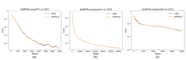
G.3 Experiments about Omitting term in Eq. (3)
We conducted experiments on SST-2 datasets using three methods to fine-tune RoBERTa-large to compare the difference between with term and without this term. Figure 13 shows that this term can make negligible influence.