Covariance-Adaptive Least-Squares Algorithm
for Stochastic Combinatorial Semi-Bandits

Abstract

We address the problem of stochastic combinatorial semi-bandits, where a player can select from $P$ subsets of a set containing $d$ base items. Most existing algorithms (e.g. CUCB, ESCB, OLS-UCB) require prior knowledge on the reward distribution, like an upper bound on a sub-Gaussian proxy-variance, which is hard to estimate tightly. In this work, we design a variance-adaptive version of OLS-UCB, relying on an online estimation of the covariance structure. Estimating the coefficients of a covariance matrix is much more manageable in practical settings and results in improved regret upper bounds compared to proxy-variance-based algorithms. When covariance coefficients are all non-negative, we show that our approach efficiently leverages the semi-bandit feedback and provably outperforms bandit feedback approaches, not only in exponential regimes where $P\gg d$ but also when $P\leq d$, which is not straightforward from most existing analyses.

Keywords— Covariance-Adaptive; Bandits; Stochastic Combinatorial Semi-Bandit; Confidence Ellipsoid

1 Introduction

In sequential decision-making, the bandit framework has been extensively studied and was instrumental to several applications, e.g. A/B testing Guo et al., (2020), online advertising and recommendation services Zeng et al., (2016), network rooting Tabei et al., (2023), demand-side management Brégère et al., (2019), etc. Its popularity stems from its relative simplicity, allowing it to model and analyze a wide range of challenging real-world settings. Reference books like Bubeck and Cesa-Bianchi, (2012) or Lattimore and Szepesvári, (2020) offer a wide perspective on the subject.

In this framework, a decision-maker or player must make choices and receives associated rewards, but it lacks prior knowledge of its environment. This naturally leads to an exploration-exploitation trade-off: the player must explore different actions to determine the best one, but an inefficient exploration strategy harms the cumulative rewards. Efficient algorithms rely on exploiting the environment’s structure, such as estimating parameters of a reward function rather than exploring every action.

In this paper, we focus on the stochastic combinatorial semi-bandit framework. In this setting, the player chooses a subset of base items and receives a feedback for each item chosen. The corresponding action set is included in the base items’ power set, and can therefore be exponentially big and difficult to explore. However, it exhibits some structure that can be leveraged. The information collected by choosing different intersecting subsets can be shared, but the way to do it efficiently over time remains a challenging problem.

Actions $\mathcal{A}\subseteq\{0,1\}^{d}$	Items $\{1,\ldots,d\}$
	Rewards $Y_{t}=(Y_{t,1},\ldots,Y_{t,d})$

Figure 1: Stochastic combinatorial semi-bandit setting where $d=3$, $\mathcal{A}=\{(0,1,0),(1,1,1),(0,1,1)\}$, and $P=|\mathcal{A}|=3$.

Problem formulation.

We consider a set of $d\in\mathbb{N}^{*}$ base items, each item $i\in[d]=\{1,\dots,d\}$ yielding stochastic rewards. A player, the decision-maker, accesses these rewards through a set $\mathcal{A}\subseteq\{0,1\}^{d}$ of $P=|\mathcal{A}|\in\mathbb{N}^{*}$ actions, each corresponding to a subset of items. We refer to actions $a\in\mathcal{A}$ using their components vectors $a=(a_{i})_{i\in[d]}\in\{0,1\}^{d}$ where for all $j\in[d]$, $a_{j}=1$ if and only if action $a$ contains base item $j$ (see Figure 1).

The player interacts with an environment over a sequence of $T\in\mathbb{N}^{*}$ rounds. At each round $t\in[T]$, the player chooses an action $A_{t}\in\mathcal{A}$, the environment samples a reward vector $Y_{t}\in\mathbb{R}^{d}$, the decision-maker observes the realization for every item contained in $A_{t}$, and receives their sum. The interactions between the player and the environment are summarized in Framework 1.

The objective of the decision-maker is to maximize the cumulative expected rewards, or equivalently, to minimize the expected cumulative regret defined as:

$$\mathbb{E}[R_{T}]=T\langle a^{*},\mu\rangle-\sum_{t=1}^{T}\mathbb{E}\big{[}\langle A_{t},Y_{t}\rangle\big{]}=\sum_{t=1}^{T}\mathbb{E}\big{[}\Delta_{A_{t}}\big{]}\,,$$ (1)

where $\langle\cdot,\cdot\rangle$ denotes the usual inner product in $\mathbb{R}^{d}$, $a^{*}\in\operatorname*{arg\,max}_{a\in\mathcal{A}}\langle a,\mu\rangle$ is an optimal action, and $\Delta_{a}=\langle a^{*}-a,\mu\rangle$ is the sub-optimality gap for $a\in\mathcal{A}$.

Framework 1 Stochastic Combinatorial Semi-Bandit

  For each $t\in\{1,\dots,T\}$:

  

• The player chooses an action $A_{t}\in\mathcal{A}$.

  

• The environment samples a vector of rewards $Y_{t}\in\mathbb{R}^{d}$ from a fixed unknown distribution.

  

• The player receives the reward

  $\langle A_{t},Y_{t}\rangle=\sum_{i}A_{t,i}Y_{t,i}$.

  

• The player observes $Y_{t,i}$ for all $i\in[d]$ s.t. $A_{t,i}=1$.

Assumptions.

We make the following assumptions on the reward $Y_{t}$. For all $t\in[T]$, $Y_{t}$ is independent of $\mathcal{F}_{t-1}=\sigma(Y_{1},\dots,Y_{t-1})$ and $A_{t}$ is $\mathcal{F}_{t-1}-$measurable. There exists a mean reward vector $\mu\in\mathbb{R}^{d}$ and a positive semi-definite covariance matrix $\mathbf{\Sigma}^{*}\in M_{d}(\mathbb{R})$ such that $\mathbb{E}[Y_{t}]=\mu\in\mathbb{R}^{d}$ and $\mathrm{Var}(Y_{t})=\mathbf{\Sigma}^{*}$. There exists a known bounds vector $B\in\mathbb{R}_{+}^{d}$ such that for all $i\in[d]$, $|Y_{t,i}-\mu_{i}|\leq B_{i}$.

Table 1: Asymptotic $\tilde{O}(\cdot)$ regret bounds for different types of feedback, up to poly-logarithmic terms in $T$ and $d$, for the following algorithms: UCB Auer et al., 2002a , UCBV Audibert et al., (2009), CUCB Kveton et al., (2015), OLS-UCB Degenne and Perchet, (2016), ESCB-C Perrault et al., (2020), and OLS-UCBV (ours). The top of the table concerns algorithms using bandit feedbacks, and the bottom algorithms exploiting semi-bandit ones. Notations: $a$ refers to actions; $i$ and $j$ refer to items; $m$ denotes the maximum number of items per action; $\Gamma$ is a proxy-covariance matrix; $\gamma$ is a maximum of ”proxy-correlations”; we abbreviate $\max\{x,0\}$ to $(x)_{+}$ for any $x\in\mathbb{R}$.

Feedback	Algorithm	Info.	Gap-Dependant Asymptotic Regret	Gap-Free Asymptotic Regret
Bandit	UCB	$\Gamma$	$\sum_{a}\frac{a^{\top}\Gamma a}{\Delta_{a}}$	$\sqrt{T\sum_{a}a^{\top}\Gamma a}$
	UCBV	$\varnothing$	$\sum_{a}\frac{a^{\top}\mathbf{\Sigma}^{*}a}{\Delta_{a}}$	$\sqrt{T\sum_{a}a^{\top}\mathbf{\Sigma}^{*}a}$
Semi-Bandit	CUCB	$\Gamma$	$m\sum_{i}\frac{\Gamma_{i,i}}{\min_{a/i\in a}\Delta_{a}}$	$\sqrt{mT\sum_{i}\Gamma_{i,i}}$
	OLS-UCB	$\Gamma$	$(1+\gamma m)\sum_{i}\frac{\Gamma_{i,i}}{\min_{a/i\in a}\Delta_{a}}+\frac{dm^{2}\max_{i}\Gamma_{i,i}}{\Delta_{\textrm{min}}^{2}}$	$(dm^{2}\max_{i}\Gamma_{i,i})^{1/3}T^{2/3}$
	ESCB-C	$\varnothing$	$\sum_{i}\max_{a/i\in a}\frac{\sum_{j\in a}(\mathbf{\Sigma}^{*}_{i,j})_{+}}{\Delta_{\textrm{min}}}+\frac{dm^{2}\max_{i}\Gamma_{i,i}}{\Delta_{\textrm{min}}^{2}}$	$(dm^{2}\max_{i}\Gamma_{i,i})^{1/3}T^{2/3}$
	OLS-UCBV	$\varnothing$	${\sum_{i}\max_{a/i\in a}\frac{\sum_{j\in a}(\mathbf{\Sigma}^{*}_{i,j})_{+}}{\Delta_{a}}}$	${\sqrt{T\sum_{i}\max_{a/i\in a}\sum_{j\in a}(\mathbf{\Sigma}^{*}_{i,j})_{+}}}$

Contributions.

One of the weaknesses of most existing algorithms for stochastic combinatorial semi-bandits is their reliance on information about the reward distribution. For example, it is common to assume the existence and knowledge of a positive semi-definite proxy-covariance matrix $\Gamma$, such that for all $t\geq 1$ and for all $u\in\mathbb{R}^{d}$, $\mathbb{E}[\exp(u^{\top}(Y_{t}-\mu))]\leq\exp(\smash{\frac{1}{2}}u^{\top}\Gamma u)$, like for OLS-UCB in Degenne and Perchet, (2016). As the performances of these algorithms explicitly involve this information, it is essential to use the tightest estimates possible. For example, when all the rewards are bounded by $B_{\text{max}}>0$, a rough proxy-covariance $\Gamma=dB_{\text{max}}^{2}\mathrm{I}_{d}$ can be provided. However, this bound is typically very loose: it poorly uses the structure of the reward distribution and results in sub-optimal guarantees. Estimating a good proxy-variance is actually a challenging problem especially when dealing with non-Gaussian distributions. We propose instead an algorithm relying on the “real” covariance matrix of the reward distribution which is easier to estimate with good theoretical guarantees.

The literature concerning stochastic combinatorial semi-bandit settings also mostly focuses on cases where the action set is exponentially large, namely $P\gg d$, and the way to get quasi-optimal regret rates in these instances. However, outside of these regimes, the commonly derived regret bounds are too rough and fail to show the benefit of the semi-bandit feedback. Conventional combinatorial semi-bandit regret upper bounds grow as $O(\sqrt{mdT})$, where $m$ is the maximum number of items per action Kveton et al., (2015), while a rate of order $O(\sqrt{mPT})$ can be achieved using bandit feedback only (for multi-armed bandit with $P$ arms and rewards having variance $m$). Intriguingly, the latter appears to outperform the semi-bandit rate as soon as $P<d$, making the extra information obtained through supplementary feedback seemingly useless. It is thus natural to look for more fine-grained analyses showing clear improvements when going from pure bandit to semi-bandit feedbacks, in all regimes.

Hereafter are listed our contributions.

• In Section 2, we show a gap-free lower bound on the regret for stochastic combinatorial semi-bandits, explicitly involving the structure of the problem (the items in each action) and the covariance matrix $\mathbf{\Sigma}^{*}$.

• In Section 3 and Section 4, we design and analyze OLS-UCBV, a least-squares-based algorithm estimating the covariance matrix online. We show that it satisfies logarithmic regret rates explicitly involving $\mathbf{\Sigma}^{*}$ and the structure of the action set $\mathcal{A}$. A good estimation of $\mathbf{\Sigma}^{*}$ is not only much simpler to get than a proxy-covariance for any reward distributions, but also provides improved regret guarantees. We show that this algorithm yields a similar gap-dependant regret bound as ESCB-C from Perrault et al., (2020), up to logarithmic factors, and an improved $\sqrt{T}$ gap-free regret bound. The corresponding regret bounds are summarized in blue in Table 1. We also show that under mild conditions, leveraging the semi-bandit feedback indeed consistently offers an advantage and outperforms bandit algorithms in all regimes of $P/d$.

• Lastly Section 5 compares the computational complexities of OLS-UCBV with existing algorithms. We particularly show that OLS-UCBV is computationally cheaper than ESCB-C as we circumvent the need to solve a convex optimization problem at each round with increasing accuracy, by relying on closed-form expressions. Algorithm performances are compared on synthetic environments in Appendix E.

Related works.

The combinatorial bandit setting has been introduced in Chen et al., (2013) which proposes CUCB (Combinatorial UCB), later analyzed in Kveton et al., (2015). This algorithm plugs upper confidence bounds for the items’ rewards into a linear maximization problem and picks the action with the highest upper bound. However this version does not exploit correlations between the different base items. Its regret bound has later been outperformed in Combes et al., (2015) and Degenne and Perchet, (2016). These papers propose algorithms than rely on the knowledge of either the parametric form of the rewards (Bernoulli in Combes et al.,, 2015) or a sub-Gaussian proxy-covariance matrix Degenne and Perchet, (2016). However, needing a proxy-covariance matrix is a major limitation as getting tight estimates is difficult in practice, and using a loose one severely impacts the performance.

While Audibert et al., (2009) designs and analyses UCBV for multi-armed bandit, Perrault et al., (2020) recently proposed ESCB-C, a covariance-adaptive algorithm for stochastic combinatorial semi-bandit. It is based on estimations of the covariance matrix and solving linear optimization problems in convex sets to compute the best action. The algorithm notably satisfies gap-dependant regret bounds depending asymptotically on the covariance matrix and solves most limitations from the previous work of Degenne and Perchet, (2016).

We propose and analyse a novel algorithm based on a least-squares estimator, closer to OLS-UCB (Degenne and Perchet,, 2016) than to ESCB-C (Perrault et al.,, 2020). We manage to show similar regret rates as Perrault et al., (2020), up to logarithmic factors, but using a different approach. In contrast to the i.i.d assumption needed in Perrault et al., (2020), our analysis only needs sequential independence and uses tools from martingales theory, which could enable easier extensions to richer settings like Markov Decision Processes. We also manage to get an improved $\tilde{O}(\sqrt{T})$ gap-free regret rate, while a $1/\Delta_{\textrm{min}}^{2}$ term in the analysis of both OLS-UCB and ESCB-C prevents it. Besides, we also gain on computational complexity over ESCB-C as we do not rely on the approximate resolution of an optimization problem to determine upper bounds on actions’ rewards.

Our analysis of OLS-UCBV is close to the one in Degenne and Perchet, (2016) but uses different concentration bounds. We draw inspiration from Zhou et al., (2021), who recently adapted martingale arguments from Dani et al., (2008). Our work however improves on Zhou et al., (2021) through the exploitation of a multi-dimensional noise covariance structure for $Y_{t}$. It requires us to tailor an analysis capable of coupling it with the peeling trick used in Degenne and Perchet, (2016). Thanks to these concentration arguments we can bound a “noise” factor in the cumulative regret, and use the same kind of “deterministic” analysis as in Kveton et al., (2015) to get logarithmic regret rates depending on the covariance matrix and the structure of the action set.

2 Lower Bound

In their recent paper, Perrault et al., (2020) prove a gap-dependant lower bound on the cumulative regret, and provide ESCB-C, an algorithm satisfying it, up to some assumptions and constant terms.

Theorem 2.1 (Theorem 1 in Perrault et al.,, 2020).

Let $d,m\in\mathbb{N}^{*}$ such that $d/m\geq 2$ is an integer, $\mathbf{\Sigma}^{*}\succeq 0$, $\delta\in(0,1)$ and a consistent policy $\pi$, such that for any combinatorial semi-bandit instance

$$\mathbb{E}[R_{T}]=o(T^{b})\quad\text{ for any }b>0\,,$$

as $T\rightarrow\infty$. Then, there exists a stochastic combinatorial semi-bandit with $d$ base items, actions of size at most $m$, and a reward distribution with covariance matrix $\mathbf{\Sigma}^{*}$ where all suboptimal gaps are $\Delta$, on which the regret satisfies

$$\liminf_{T\rightarrow\infty}\frac{\Delta}{\log(T)}R_{T}\geq 2\sum_{i\in[d],i\notin a^{*}}\max_{a\in\mathcal{A},i\in a}\sum_{j\in a}\mathbf{\Sigma}^{*}_{i,j}\,.$$

Their proof considers $d/m$ disjoint actions, with Gaussian rewards, and a reduction to a multi-armed bandit’s lower bound. For a similar type of instance, we introduce a novel gap-free lower bound.

Theorem 2.2.

Let $d,m\in\mathbb{N}^{*}$ such that $d/m\geq 2$ is an integer, $T\in\mathbb{N}^{*}$, and $\mathbf{\Sigma}^{*}\succeq 0$ a covariance matrix. Then, there exists a stochastic combinatorial semi-bandit with $d$ base items, actions of size at most $m$, and a reward distribution with covariance matrix $\mathbf{\Sigma}^{*}$ on which for any policy $\pi$, the regret satisfies

$$R_{T}\geq\frac{1}{8}\sqrt{T\sum_{i\in[d]}\max_{a\in\mathcal{A},i\in a}\sum_{j\in a}\mathbf{\Sigma}^{*}_{i,j}}\,.$$

Proof.

The proof is detailed in Section A.1. We follow the methodology of Auer et al., 2002b , modifying it to account for the different variances among actions. ∎

3 OLS-UCBV

In this section, we design a new algorithm that efficiently leverages the semi-bandit feedback by approximating the coefficients of the covariance matrix $\mathbf{\Sigma}^{*}$ online. This approximation is symmetric by construction and yields a coefficient-wise upper bound of $\mathbf{\Sigma}^{*}$. But it is not necessarily a semi-definite positive matrix, a constraint that can be extremely challenging to tightly impose in practical scenarios.

While Perrault et al., (2020) use an axis-realignment technique and a covering argument to derive their confidence region, our approach is closer to the least-squares methodology of Degenne and Perchet, (2016). It uses ellipsoidal confidence regions in which we incorporate Bernstein-like concentration inequalities. This particularly simplifies the computation of an upper confidence bound for each action. While Perrault et al., (2020) need to solve linear programs in convex sets at each iteration to derive their bound, we have access to closed-form expressions. More details on these differences in complexity are given in Section 5.

3.1 Estimators for mean and covariance

Mean estimation.

Let $a\in\mathcal{A}$, $t\in[T]$, we denote by $\mathbf{d}_{a}=\mathrm{diag}(a)\in M_{d}(\mathbb{R})$ the diagonal matrix where the non-null coefficients are the elements of $a$. The number of times two items $i,j\in[d]$ (with possibly $i=j$) have been chosen together after round $t$ is denoted by $\smash{n_{t,(i,j)}=\sum_{s=1}^{t}\mathds{1}\big{\{}(i,j)\in A_{s}\big{\}}}$. We define $\mathbf{D}_{t}=\mathrm{diag}((n_{t,(i,i)})_{i\in[d]})\in M_{d}(\mathbb{R})$ the diagonal matrix of item counts. Then the least-squares estimator dor the mean reward vector $\mu$ using all the data from the past rounds after round $t$ is the empirical average

$$\textstyle\hat{\mu}_{t}=\mathbf{D}_{t}^{-1}\sum_{s=1}^{t}\mathbf{d}_{A_{s}}Y_{s}=\mu+\mathbf{D}_{t}^{-1}\sum_{s=1}^{t}\mathbf{d}_{A_{s}}\eta_{s}\,,$$ (2)

where $\eta_{s}$ denotes the deviation of reward $Y_{s}$ from its mean $\mu$. This average yields the estimator $\langle a,\hat{\mu}_{t}\rangle$ for the mean reward $\langle a,\mu\rangle$, to which a well-designed optimistic bonus should be added. We design a strategy inspired from LinUCB (Rusmevichientong and Tsitsiklis,, 2010; Filippi et al.,, 2010). The ellipsoid-based bonus that we introduce enables the use of a peeling trick and Bernstein’s style concentration inequalities.

Covariance estimation.

Let $t\in\mathbb{N}^{*}$ and $i,j\in[d]$ such that $n_{t,(i,j)}\geq 2$. The coefficients of $\mathbf{\Sigma}^{*}$ can be estimated online by $\hat{\chi}_{t}$ with elements as follows

$$\hat{\chi}_{t,(i,j)}=\textstyle\frac{1}{n_{t,(i,j)}}\sum_{s=1}^{t}A_{s,i}A_{s,j}\mathds{1}\{n_{s,(i,j)}\geq 2\}(Y_{s,i}-\hat{\mu}_{s-1,i})(Y_{s,j}-\hat{\mu}_{s-1,j})\,.$$ (3)

A major difference with the estimators used in Perrault et al., (2020) (or those used in Audibert et al.,, 2009) is the fact that the rewards are “centered” using the sample average of the past rewards at the time of their observation ($s$ in our case), instead of the whole sample average at time $t$.

3.2 Upper confidence bounds for covariance and mean

Covariance coefficients upper confidence bound.

The following result controls the error of the online covariance estimator $\hat{\chi}_{t}$ presented in Equation 3.

Proposition 3.1.

Let $T\geq 3$, $\delta\in(0,1)$. Then with probability $1-\delta$, for all $t\leq T$ and $(i,j)\in[d]^{2}$, such that $n_{t,(i,j)}\geq 2$,

$$|\hat{\chi}_{t,(i,j)}-\mathbf{\Sigma}^{*}_{i,j}| \leq\mathcal{B}_{t,(i,j)}(\delta,T)\,,$$

where $\mathcal{B}_{t,(i,j)}(\delta,T)=3B_{i}B_{j}\left(\frac{h_{T,\delta}}{\sqrt{n_{t,(i,j)}}}+\frac{h_{T,\delta}^{2}}{n_{t,(i,j)}}\log(T)\right)$ with $h_{T,\delta}=\log(5d^{2}T^{2}/\delta)$.

Proof.

See Section B.1. ∎

This result suggests the following upper confidence bounds for $\mathbf{\Sigma}^{*}$ to be plugged into our algorithm:

$$\hat{\mathbf{\Sigma}}_{t,(i,j)} =\hat{\chi}_{t,(i,j)}+\mathcal{B}_{t,(i,j)}(\delta,T)\,.$$ (4)

Mean upper confidence bound.

We propose an upper confidence bound for the average rewards of all actions $a\in\mathcal{A}$ at any round $t$.

Denoting by $\hat{\mathbf{\Sigma}}_{t}$ the coefficient-wise UCB covariance matrix given by (4), we introduce the following “regularized empirical design matrix”:

$$\textstyle\hat{\mathbf{Z}}_{t} =\sum_{s=1}^{t}\mathbf{d}_{A_{s}}\hat{\mathbf{\Sigma}}_{t}\mathbf{d}_{A_{s}}+\mathbf{d}_{\hat{\mathbf{\Sigma}}_{t}}\mathbf{D}_{t}+d\mathbf{d}_{B}\,,$$ (5)

where $\smash{\mathbf{d}_{B}=\mathrm{diag}((B_{i}^{2})_{i\in[d]})}$ and $\smash{\mathbf{d}_{\hat{\mathbf{\Sigma}}_{t}}=\mathrm{diag}(\hat{\mathbf{\Sigma}}_{t})}$ are matrices in $M_{d}(\mathbb{R})$. The regularization of the matrix $\hat{\mathbf{Z}}_{t}$ is engineered to enable the use of a peeling trick in the proof of the regret bound stated in Theorem 3.2.

As we show in the upcoming analysis (see proof of Proposition 4.5), with probability greater than $1-\delta$, for all $a\in\mathcal{A}$

$$|\langle a,\mu\rangle-\langle a,\hat{\mu}_{t}\rangle|\leq f_{t,\delta}\ \|\mathbf{D}_{t}^{-1}a\|_{\mathbf{Z}_{t}}\,,$$

where

$$f_{t,\delta}=6d\log\big{(}\log(1+t)\big{)}+3d\log(1+e)+\log(1/\delta)\,,$$ (6)

is an exploration factor depending on the desired uncertainty level $\delta\in(0,1)$ and $\mathbf{Z}_{t}$ is the “exact” counterpart of $\hat{\mathbf{Z}}_{t}$, using $\mathbf{\Sigma}^{*}$ instead of $\hat{\mathbf{\Sigma}}_{t}$.

3.3 Algorithm

We now present OLS-UCBV written in Algorithm 2.

The algorithm first performs an initial exploration by sampling every base item $i\in[d]$ and every “reachable” couple $(i,j)\in[d]^{2}$ at least twice. Then, for all subsequent rounds $t+1$, OLS-UCBV picks an action $A_{t+1}$ such that:

$$A_{t+1}\in\!\operatorname*{arg\,max}_{a\in\mathcal{A}}\Big{\{}\langle a,\hat{\mu}_{t}\rangle+f_{t,\delta}\ \big{\|}\mathbf{D}_{t}^{-1}a\big{\|}_{\hat{\mathbf{Z}}_{t}}\Big{\}}\,.\vspace*{-8pt}$$ (7)

Algorithm 2 OLS-UCBV

  Input $\delta>0$, $T\geq 1$, $B\in\mathbb{R}_{+}^{d}$.

  for $t=1,\dots,T$ do

     if $\big{\{}a\in\mathcal{A}\text{ s.t }\min_{(i,j)\in a}n_{t,(i,j)}\leq 1\big{\}}\neq\emptyset$ then

        Choose any $A_{t}$ in the above set.

     else

        Choose $A_{t}\in\mathcal{A}$ from (7) using $\hat{\mu}_{t-1},\hat{\mathbf{Z}}_{t-1}$.

        Environment samples $Y_{t}\in\mathbb{R}^{d}$.

        Receive reward $\langle A_{t},Y_{t}\rangle=\sum_{i}A_{t,i}Y_{t,i}$.

        Compute $\hat{\mu}_{t}$ from (2).

        Compute $\hat{\mathbf{\Sigma}}_{t}$ from (3) and (4).

        Compute $\hat{\mathbf{Z}}_{t}$ from (5).

     end if

  end for

3.4 Regret upper bound

We establish the following regret upper bounds for OLS-UCBV. We denote $\tilde{O}$ for $O$ when $T\rightarrow\infty$, up to poly-logarithmic terms.

Theorem 3.2.

Let $T\geq 5$, $B\in\mathbb{R}_{+}^{d}$, and $\delta=1/T^{2}$. Let

$$\sigma_{a,i}^{2}=\sum_{j\in a}(\mathbf{\Sigma}^{*}_{i,j})_{+}\,,$$ (8)

where $i\in[d]$, $a\in\mathcal{A}$ and $(\,\cdot\,)_{+}=\max\{\cdot,0\}$. Then, OLS-UCBV (Alg. 2) satisfies the gap-dependent regret upper bound

$$\mathbb{E}[R_{T}]=\tilde{O}\Bigg{(}\log(d)^{2}\sum_{i=1}^{d}\max_{a\in\mathcal{A}/i\in a,\Delta_{a}>0}\frac{\sigma_{a,i}^{2}}{\Delta_{a}}\Bigg{)}\,,$$

and the distribution-free regret upper bound

$$\textstyle\mathbb{E}[R_{T}]=\tilde{O}\bigg{(}\log(d)\sqrt{\textstyle T\sum_{i=1}^{d}\max\limits_{a\in\mathcal{A}/i\in a}\sigma_{a,i}^{2}}\bigg{)}\,.$$

We manage to get the same gap-dependent regret upper bound as ESCB-C Perrault et al., (2020), up to logarithmic factors in time but we also manage to get a new $\sqrt{T}$ gap-free bound.

Diagonal covariance.

It is important to note that in the scenario of independent item rewards, where the covariance $\mathbf{\Sigma}^{*}$ is diagonal, then $\sigma_{a,i}^{2}=\Sigma^{*}_{i,i}$ for all $a\in\mathcal{A}$ and $i\in a$. Our gap-dependent and gap-free upper bounds are then roughly bounded as

$$\tilde{O}\bigg{(}\sum_{i=1}^{d}\frac{\Sigma^{*}_{i,i}}{\min\limits_{a\in\mathcal{A}/i\in a}\Delta_{a}}\bigg{)}\ \text{and}\ \textstyle\tilde{O}\Big{(}\sqrt{\mathrm{Tr}(\mathbf{\Sigma}^{*})T}\Big{)}\,,$$

respectively. In this particular case, our gap-free bound outperforms the standard regret upper bound for combinatorial semi-bandit problems (which does not use the independence information, see for instance Kveton et al., (2015)), typically of the order $O(\sqrt{dmT})$ where $m$ is the maximum number of items per action.

4 Analysis of OLS-UCBV

In this section, we analyze OLS-UCBV by detailing key steps of the proof of Theorem 3.2, while certain technical arguments are deferred to Appendix C.

The proof relies on considering high-probability “favorable” events where the two following conditions are met:

• $\hat{\mu}_{t}$ remains within a sufficiently small ellipsoid, the size of which expands logarithmically over time with $f_{t,\delta}$ – denoted as $\mathcal{G}_{t}$ thereafter, see (9),

• the covariance estimators are within high confidence bounds as specified in Proposition 3.1 – denoted as $\mathcal{C}$ thereafter, see (10).

4.1 Defining “favorable” events

Let $t\in[T]$ and $a\in\mathcal{A}$. We introduce the regularized design matrix $\mathbf{Z}_{t}$ using the covariance matrix $\mathbf{\Sigma}^{*}$ (recall the empirical version defined in (5))

$$\textstyle\mathbf{Z}_{t}=\sum_{s=1}^{t}\mathbf{d}_{A_{s}}{\mathbf{\Sigma}}^{*}\mathbf{d}_{A_{s}}+\mathbf{d}_{{\mathbf{\Sigma}}^{*}}\mathbf{D}_{t}+d\mathbf{d}_{B}\,,$$

and the event

$$\textstyle\mathcal{G}_{t}=\big{\{}\ \big{\|}\sum_{s=1}^{t}\mathbf{d}_{A_{s}}\eta_{s}\big{\|}_{\mathbf{Z}_{t}^{-1}}\leq f_{t,\delta}\big{\}}\,,$$ (9)

corresponding to the belonging of $\hat{\mu}_{t}$ to an ellipsoid centered in $\mu$ (since $\eta$ denote rewards deviations from the mean $\mu$), the size of which grows with $f_{t,\delta}$ given in (6). We also define the event $\mathcal{C}$ of Proposition 3.1 as

$$\mathcal{C}=\Big{\{}\forall t\in[T],\ (i,j)\in[d]^{2}\text{ s.t. }n_{t,(i,j)}\geq 2,|\hat{\chi}_{t,(i,j)}-\mathbf{\Sigma}^{*}_{i,j}|\leq\mathcal{B}_{t,(i,j)}(\delta,T)\Big{\}}\,,$$ (10)

having probability at least $1-\delta$.

4.2 Regret template bound

The algorithm begins with an exploration phase lasting at most $d(d+1)$ rounds. Thus,

$$\textstyle\mathbb{E}[R_{T}]\leq d(d+1)\Delta_{\mathrm{max}}+\sum_{t=d(d+1)}^{T-1}\mathbb{E}[\Delta_{A_{t+1}}],$$ (11)

where $\Delta_{\mathrm{max}}$ is the largest suboptimality gap in the instance.

Using the fact that the probability of $\mathcal{C}$ is at least $1-\delta$, the formula of total probability brings

$$\mathbb{E}[R_{T}] \leq\Delta_{\mathrm{max}}\Big{(}d(d+1)+\underbrace{\sum_{t=d(d+1)}^{T-1}\mathbb{P}\big{(}\mathcal{G}_{t}^{c}\big{)}}_{\mathbf{A}}+T\delta\Big{)}+\underbrace{\sum_{t=d(d+1)}^{T-1}\mathbb{E}\Big{[}\Delta_{A_{t+1}}\mathds{1}\{\mathcal{G}_{t}\bigcap\mathcal{C}\}\Big{]}}_{\mathbf{B}}\,.$$ (12)

The rest of the proof consists in upper bounding the terms $\mathbf{A}$ and $\mathbf{B}$ appearing in (12), for which we now provide respective sketches of proof.

4.3 Bounding $\mathbf{A}=\sum_{t=d(d+1)}^{T-1}\mathbb{P}\big{(}\mathcal{G}_{t}^{c}\big{)}$

The term ${\mathbf{A}=\sum_{t=d(d+1)}^{T-1}\mathbb{P}\big{(}\mathcal{G}_{t}^{c}\big{)}}$ upper-bounds the probability that at least one of the unfavorable events $\mathcal{G}_{t}^{c}$ is realized –i.e. that for at least one round $t$, $\hat{\mu}_{t}$ is outside of the ellipsoid defined by (9). The following result provides an upper bound for $\mathbf{A}$.

Proposition 4.1.

For events $\{\mathcal{G}_{t}\}_{t\leq T}$ defined as in (9), we have

$$\textstyle\sum_{t=d(d+1)}^{T-1}\mathbb{P}\big{(}\mathcal{G}_{t}^{c}\big{)}\leq\delta T^{2}.$$ (13)

Proof.

Bounding $\sum_{t=d(d+1)}^{T-1}\mathbb{P}\big{(}\mathcal{G}_{t}^{c}\big{)}$ needs a meticulous interaction of a peeling trick as used by Degenne and Perchet, (2016) and martingale arguments inspired from Abbasi-Yadkori et al., (2011). In the next two paragraphs, we present the main results of each of these two elements of the proof.

Peeling trick.

The peeling trick consists in separating the space of trajectories up to round $t$ into an exponentially large number of parts, each having an exponentially small probability.

Formally, let $\epsilon>0$. To each $p\in\mathbb{N}^{d}$ we associate the set

$$\mathcal{D}_{p}=\big{\{}x\in \mathbb{R}^{d}\text{ s.t. }\forall i\in[d],\ (1+\epsilon)^{p_{i}}\leq x_{i}<(1+\epsilon)^{p_{i}+1}\big{\}}\,.$$ (14)

As an abuse of notation, we denote by $(t\in\mathcal{D}_{p})$ the event $((n_{t,(i,i)}+1)_{i\in[d]}\in\mathcal{D}_{p})$.

Setting $P_{t,\epsilon}=\big{\lfloor}\frac{\log(1+t)}{\log(1+\epsilon)}\big{\rfloor}$, we define for each $p\in[P_{t,\epsilon}]^{d}$

$$\mathbf{D}_{p} =\mathrm{diag}\Big{(}\big{(}(1+\epsilon)^{p_{i}}\big{)}_{i\in[d]}\Big{)}\in M_{d}(\mathbb{R})\,,$$

$$\mathbf{Z}_{t,p} =\sum_{s=1}^{t}\mathbf{d}_{A_{s}}\mathbf{\Sigma}^{*}\mathbf{d}_{A_{s}}+\mathbf{d}_{\mathbf{\Sigma}^{*}}\mathbf{D}_{p}+d\mathbf{d}_{B}\,,$$

$$M_{t,p} =\bigg{\|}\sum_{s=1}^{t}\mathbf{d}_{A_{s}}\eta_{s}\bigg{\|}_{\mathbf{Z}_{t,p}^{-1}}\,.$$ (15)

Proposition 4.2.

With the notations of (14) and (15), we have

$$\mathbb{P}(\mathcal{G}_{t}^{c})\leq\sum_{p\in[P_{t,\epsilon}]^{d}}\mathbb{P}\Big{\{}(M_{t,p}^{2}>f_{t,\delta}^{2})\bigcap(t\in\mathcal{D}_{p})\Big{\}}\,.$$ (16)

Proof.

The proof is deferred to Appendix C.1. ∎

Martingale bounding.

The following result proposes a bound for the right-hand side of (16) and is proven using martingale arguments.

Proposition 4.3.

For $p\in[P_{t,\epsilon}]^{d}$ and with the notations of (14) and (15), we have

$$\mathbb{P}\Big{\{}M_{t,p}^{2}>f_{t,\delta}^{2}\bigcap(t\in\mathcal{D}_{p})\Big{\}}\leq 2t\delta\left(\frac{\log(1+\epsilon)}{\log(1+t)}\right)^{d}\,,$$ (17)

where $f_{t,\delta}=6d\log(\log(1+t))+3d\log(1+e)+\log(1/\delta)$ is defined in (6).

Proof.

The proof is deferred to Appendix C.2. ∎

Armed with Propositions 4.2 and 4.3 we can finally write:

$$\mathbb{P}(\mathcal{G}_{t}^{c})\stackrel{{\scriptstyle\eqref{eq:peeling-trick-main-bound}}}{{\leq}}\sum_{p\in[P_{t,\epsilon}]^{d}}\mathbb{P}\Big{\{}M_{t,p}^{2}>f_{t,\delta}^{2}\bigcap(t\in\mathcal{D}_{p})\Big{\}}\stackrel{{\scriptstyle\eqref{eq:martingale-bound}}}{{\leq}}(P_{t,\epsilon})^{d}2t\delta\left(\frac{\log(1+\epsilon)}{\log(1+t)}\right)^{d}\leq 2t\delta\,,$$

where the last inequality comes from $P_{t,\epsilon}=\big{\lfloor}\frac{\log(1+t)}{\log(1+\epsilon)}\big{\rfloor}$. Summing for $t=d(d+1)$ to $T-1$ then shows (13) which is the desired result. ∎

4.4 Bounding $\mathbf{B}=\sum_{t=d(d+1)}^{T-1}\mathbb{E}\big{[}\Delta_{A_{t+1}}\mathds{1}\{\mathcal{G}_{t}\bigcap\mathcal{C}\}\big{]}$

Leveraging the careful definition of the favorable $\{\mathcal{G}_{t}\}_{t\in[T]}$ and $\mathcal{C}$ from (9) and (10) enables us to provide the following result to bound term $\mathbf{B}$, corresponding the cumulative regret incurred under $\{\mathcal{G}_{t}\bigcap\mathcal{C}\}$ at each round $t$.

Our objective is to prove that $\mathrm{B}$ grows at most poly-logarithmically w.r.t. $T$, with coefficients depending on the structure of the instance and the covariance matrix $\mathbf{\Sigma}^{*}$. We state our result formally in the following proposition.

Proposition 4.4.

Let $T\geq d(d+1)$ and $\delta=1/T^{2}$. Then,

$$\mathbb{E}\bigg{[}\sum_{t=d(d+1)}^{T-1}\Delta_{A_{t+1}}\mathds{1}\big{\{}\mathcal{G}_{t}\bigcap\mathcal{C}\big{\}}\bigg{]}=O\Bigg{(}\log(T)^{3}(\log d)^{2}\Big{(}\sum_{i=1}^{d}\max_{a\in\mathcal{A}/i\in a}\frac{\sigma_{a,i}^{2}}{\Delta_{a}}\Big{)}\Bigg{)}\,,$$

as $T\rightarrow\infty$, where $\sigma_{a,i}^{2}=\sum_{j\in a}(\mathbf{\Sigma}^{*}_{i,j})_{+}$.

Proof.

We first prove the following result which gives an upper bound of the gap $\Delta_{A_{t+1}}$ under $\{\mathcal{G}_{t}\bigcap\mathcal{C}\}$.

Proposition 4.5.

Let $t\geq d(d+1)$. Then under $\{\mathcal{G}_{t}\bigcap\mathcal{C}\}$, $\Delta_{A_{t+1}}\leq f_{t,\delta}\big{(}\|\mathbf{D}_{t}^{-1}A_{t+1}\|_{\mathbf{Z}_{t}}+\|\mathbf{D}_{t}^{-1}A_{t+1}\|_{\hat{\mathbf{Z}}_{t}}\big{)}$.

Proof.

The proof is deferred to Appendix C.7. ∎

To continue with our objective to bound $\mathbf{B}$, we take inspiration from the works of Kveton et al., (2015) and Degenne and Perchet, (2016). For starters, we prove the following result (using $\bar{\sigma}_{a,i}^{2}$’s defined differently from the $\sigma_{a,i}$’s).

Lemma 4.6.

Let $t\geq d(d+1)$, we have that under $\{\mathcal{G}_{t}\bigcap\mathcal{C}\}$,

$$\frac{\Delta_{A_{t+1}}^{2}}{4f_{t,\delta}^{2}} \leq\frac{1}{2}\big{(}\|\mathbf{D}_{t}^{-1}A_{t+1}\|_{\mathbf{Z}_{t}}^{2}+\|\mathbf{D}_{t}^{-1}A_{t+1}\|_{\hat{Z}_{t}}^{2}\big{)}$$

$$\leq\sum_{i\in A_{t+1}}\frac{\bar{\sigma}_{A_{t+1},i}^{2}}{n_{t,(i,i)}}+\big{(}d+3\log(T)h_{T,\delta}^{2}\big{)}\sum_{(i,j)\in A_{t+1}}\frac{B_{i}B_{j}}{n_{t,(i,j)}^{2}}+3h_{T,\delta}\sum_{(i,j)\in A_{t+1}}\frac{B_{i}B_{j}}{n_{t,(i,j)}^{3/2}}\,,$$ (18)

where

$$\bar{\sigma}_{A_{t+1},i}^{2}=2\sum_{j\in A_{t+1}/\mathbf{\Sigma}^{*}_{j,j}\leq\mathbf{\Sigma}^{*}_{i,i}}(\mathbf{\Sigma}^{*}_{i,j})_{+}\leq 2\sigma_{A_{t+1},i}^{2}\,.$$

Proof.

The proof is a consequence of Proposition 4.5 and is deferred to Appendix C.8. ∎

Unfortunately, only the positive coefficients of $\mathbf{\Sigma}^{*}$ are considered in the analysis but the inclusion of negative correlations could be advantageous to reduce the rate at which the regret increases. However, it is quite complex and thus deferred to future research.

The rest of the proof involves a decomposition of $\{\mathcal{G}_{t}\bigcap\mathcal{C}\}$. By considering each of the $3$ sub-sum in Equation 18 and designing set of event that are implied by $\{\mathcal{G}_{t}\bigcap\mathcal{C}\}$ but that can happen only a finite number of times.

In practice, we introduce two well-chosen sequences $(\alpha_{k})_{k\in\mathbb{N}}$ and $(\beta_{k})_{k\in\mathbb{N}}$ (see Section C.9), and define sequences of events $\mathbb{A}_{t,k}^{r}$ for $k\in\mathbb{N}^{*}$ and $r=1,2\text{ and }3$ from them (see Section C.10). In particular, the following result holds

Lemma 4.7.

Let $t\geq d(d+1)$ and $k_{0}\in\mathbb{N}^{*}$ such that $0<d\beta_{k_{0}}<\big{(}\frac{1}{d}\wedge\min_{i,a}\{\mathbf{\Sigma}^{*}_{i,i}\bar{\sigma}_{a,i}^{-2}\}\big{)}$. Then,

$$\textstyle\mathds{1}\{\mathcal{G}_{t}\bigcap\mathcal{C}\}\leq\sum_{r=1}^{3}\sum_{k=1}^{k_{0}}\mathds{1}\{\mathbb{A}_{t,k}^{r}\}\,.$$

Proof.

The proof is deferred to Appendix C.11. ∎

The rest of the proof consists in upper bounding $\sum_{t=d(d+1)}^{T-1}\Delta_{A_{t+1}}\mathds{1}\{\mathbb{A}_{t,k}^{r}\}$ for each $(r,k)\in[3]\times[k_{0}]$ using the definitions of the events, and is detailed in Appendix C.12.

A notable difference from previous approaches by Kveton et al., (2015); Degenne and Perchet, (2016) is the use of $\mathbf{\Sigma}_{i,i}^{*}/\bar{\sigma}_{a,i}^{2}$ in $\mathbb{A}_{t,k}^{1}$ instead of set cardinals. This enables the explicit appearance of the $\sigma_{a,i}^{2}$ coefficients (as $\bar{\sigma}_{a,i}^{2}\leq 2\sigma_{a,i}^{2}$). The use of $\log(T)$ and $\frac{2\log(T)}{\log(T)-1}$ factors for Lemma 4.7 also enable to make the terms depending on $\sigma_{a,i}^{2}$ dominant in the final bound. ∎

4.5 Conclusion of the proof

Injecting results from Proposition 4.4 and Proposition 4.1 into (12) finally yields

$$\mathbb{E}[R_{T}]=O\Bigg{(}\log(T)^{3}\Big{(}\sum_{i\in[d]}\max_{a\in\mathcal{A}/i\in a}\frac{\sigma_{a,i}}{\Delta_{a}^{\prime}}\Big{)}(\log d)^{2}\Bigg{)}\,,$$

as $T\rightarrow\infty$. This provides the gap-dependent bound of Theorem 3.2. The gap-free bound is detailed in Appendix D. It arises from the fact that our gap-dependent bound does not incur any term in $\Delta_{\mathrm{min}}^{-2}$, unlike Perrault et al., (2020); Degenne and Perchet, (2016).

5 Comparisons and Complexity Analysis

5.1 Regret rates

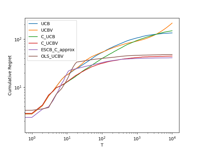
Figure 2: Average Cumulative Regret for environments generated with $d=10$ and $P=10$ and exploration parameters fine-tuned.

Some advantages of using variance-adaptive algorithms instead of ones for which the performance depends on potentially non-tight quantities like sub-Gaussian parameters have been outlined in Section 3.4 and discussed more in Audibert et al., (2009) and Perrault et al., (2020). They particularly yield regret rates that can be considerably improved, at the cost of only marginally more computations. Among stochastic combinatorial semi-bandit algorithms, OLS-UCBV thus manages to yield variance-dependant regret rates similar to those reached by Perrault et al., (2020) up to log factors, but with an additional gap-free rate evolving as $\sqrt{T}$, see Table 1. An example of experiment can be found in Figure 2 in Appendix E where we can see that OLS-UCBV yields similar regret as other combinatorial algorithms.

5.2 Computational complexity

Another point of comparison between algorithms is their computational complexity, outlined in Table 2. Combinatorial semi-bandit algorithms are known not to be efficiently manageable for big action sets in the absence of structure (matroid constraints for example). For our comparison, we place ourselves in settings where we can afford to iterate computationally over it, thus the $P$ factors. In that case, for the same theoretical guarantees, OLS-UCBV is cheaper to execute compared to ESCB-C. Indeed, the latter needs to solve a linear program in a convex set at each round for each action, and with enough precision so that it does not influence the regret substantially. Given the form of the problem, this operation is significantly more costly than computing the upper confidence bound of OLS-UCBV which has a closed form involving only a finite number of matrix operations.

5.3 Complexity / regret trade-off

We now analyze the complexity / regret trade-off between using the pure bandit feedback or using the semi-bandit one, in settings where the number of actions is reasonable. Exploiting the semi-bandit feedback may be beneficial in certain cases, as it enables to combine information collected by different actions, but this comes at the cost of an increased computational complexity which may not be worth it. Looking more precisely at the gap-free regret rates in Table 1, while the regret of UCBV is upper bounded by $\smash{\big{(}T\sum_{a}a^{\top}\mathbf{\Sigma}^{*}a\big{)}^{1/2}}$, the upper bound for OLS-UCBV is $\smash{\big{(}T\sum_{i}\max_{a/i\in a}\sum_{j\in a}({\mathbf{\Sigma}^{*}}_{i,j})_{+}\big{)}^{1/2}}$. In the case where all the correlations are positive or null, OLS-UCBV performs better. But in general, it may not be the case and negative coefficients in $\mathbf{\Sigma}^{*}$ could make $\sum_{a}a^{\top}\mathbf{\Sigma}^{*}a$ smaller than $\sum_{i}\max_{a/i\in a}\sum_{j\in a}({\mathbf{\Sigma}^{*}}_{i,j})_{+}$, particularly in cases where $P$ is not significantly bigger than $d$. Unfortunately, leveraging negative coefficients of $\mathbf{\Sigma}^{*}$ to make the semi-bandit feedback “always better” than the pure bandit feedback (as intuition dictates) does not seem to be straightforward and remains an open question.

Table 2: Complexity of the following algorithms: UCB Auer et al., 2002a , UCBV Audibert et al., (2009), CUCB Kveton et al., (2015), OLS-UCB Degenne and Perchet, (2016), ESCB-C Perrault et al., (2020), and OLS-UCBV (ours). $\text{C}_{1/T}^{\text{opt}}$ refers to the complexity of the optimisation step needed in ESCB-C.

Feed.	Algorithm	Time	Space
Bandit	UCB/UCBV	$TP$	$P$
Semi-B.	CUCB	$TPm$	$d+P$
	OLS-UCB	$T(m^{2}+Pd^{2})$	$d^{2}+P$
	ESCB-C	$T(m^{2}+P\ \text{C}_{1/T}^{\text{opt}})$	$d^{2}+P$
	OLS-UCBV	$T(m^{2}+Pd^{2})$	$d^{2}+P$

5.4 Empirical comparison

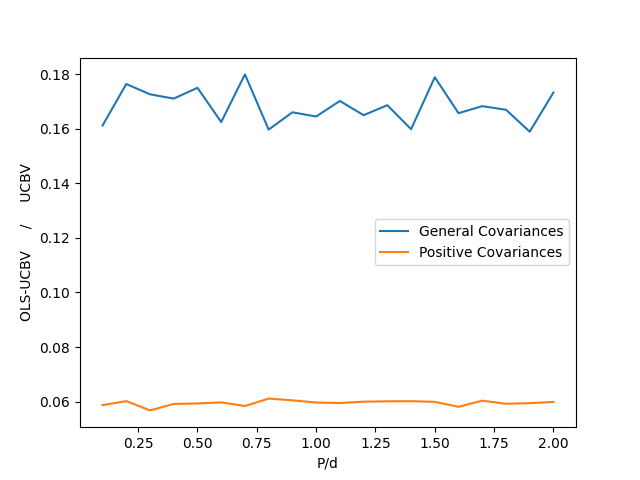
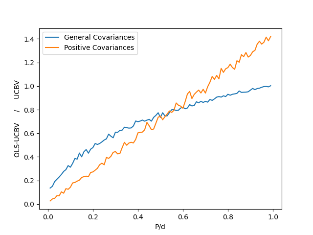
Figure 3: Comparison of the theoretical regret rate of OLS-UCBV and UCBV for a general structure on the left, and no action overlap on the right.

We compare empirically in Appendix E theoretical regret rates of UCBV and OLS-UCBV, $\big{(}\sum_{i}\max_{a/i\in a}\sigma_{a,i}\big{)}\allowbreak/\big{(}\sum_{a}a^{\top}\mathbf{\Sigma}^{*}a\big{)}$, for randomly generated instances with different ratios $P/d$. Not enforcing any particular structure, the ratio seems to remain constant for our generated instances, with a notably constant factor gain when the covariance coefficients are biased to remain positive. But when we enforce a particular structure, like actions with no overlaps, we can actually see regimes where the absence of negative coefficients in the theoretical rate of OLS-UCB is detrimental, Figure 3 in Appendix E.

6 Concluding Remarks

We propose and analyze OLS-UCBV, a covariance-adaptive algorithm for stochastic combinatorial semi-bandits. Compared to other existing approaches, ours is computationally less demanding and yields the first $\sqrt{T}$ gap-free regret rate depending explicitly on the covariance of the base items rewards. A limitation, also existing in other works, is the overlooking of negative covariance coefficients. Finding a way to take them into account might greatly improve the performances of semi-bandit algorithms and show the benefit of the additional feedback compared to a pure bandit one.

Appendix A Proofs of Section 2

A.1 Proof of Theorem 2.2

See 2.2

Proof.

Let $d,m\in\mathbb{N}^{*}$ such that $d/m\geq 2$ is an integer, $T\in\mathbb{N}^{*}$ a horizon, and $\mathbf{\Sigma}^{*}\succeq 0$ a covariance matrix. We consider the structure where $\mathcal{A}=\{a_{1},\dots,a_{d/m}\}\subset\{0,1\}^{d}$ contains $d/m$ disjoint actions each having $m$ base elements. We consider that for all $p\in[d/m]$, $\smash{(a_{p})_{i\in[d]}=\big{(}\mathds{1}\big{\{}(p-1)m<i\leq pm\big{\}}\big{)}_{i\in[d]}}$. Let $\pi$ be a policy. As all the actions are disjoints, we can reduce ourselves to a multi-armed bandit with $d/m$ actions, where for all $p\in[d/m]$ the variance of the $p$-th action is $a_{p}^{\top}\mathbf{\Sigma}^{*}a_{p}$.

Let $\mathbf{\Sigma}^{\prime}\in M_{d/m}(\mathbb{R})$ be the diagonal matrix where for all $p\in[d/m]$, $\mathbf{\Sigma}^{\prime}_{p,p}=a_{p}^{\top}\mathbf{\Sigma}^{*}a_{p}$. Let $c>0$, and

$$\Delta=2c\sqrt{\mathbf{\Sigma}^{\prime}_{\text{min}}\frac{\sum_{k=1}^{d/m}\mathbf{\Sigma}^{\prime}_{k,k}}{T}}\,,$$ (19)

where $\mathbf{\Sigma}^{\prime}_{\text{min}}=\min_{p\in[d/m]}\mathbf{\Sigma}^{\prime}_{p,p}$.

We denote $G_{0}\sim\mathcal{N}(0,\mathbf{\Sigma}^{\prime})$ a $(d/m)$-dimensional centered Gaussian distribution with covariance matrix $\mathbf{\Sigma}^{\prime}$. Let $p\in[d/m]$, we consider the mean vector $\mu^{(p)}\in\mathbb{R}^{d/m}$ having coordinate 0 everywhere and $\Delta$ at coordinate $p$, for all $i\in[d/m]$, $\mu^{(p)}_{i}=\Delta\mathds{1}\{i=p\}$. We introduce the Gaussian reward distributions $G_{p}\sim\mathcal{N}(\mu^{(p)},\mathbf{\Sigma}^{\prime})$ and denote $T_{p}=\sum_{t=1}^{T}\mathds{1}\{A_{t}=p\}$. Then, using policy $\pi$, and considering the reward distributions $G_{p}$ and $G_{0}$, the average number of times action $p$ has been chosen satisfies

$$\Big{|}\mathbb{E}_{\pi,G_{p}}[T_{p}]-\mathbb{E}_{\pi,G_{0}}[T_{p}]\Big{|}\leq T\ \mathrm{TV}\Big{(}(\pi,G_{0}),(\pi,G_{p})\Big{)}\leq T\sqrt{\frac{1}{2}\mathrm{KL}\Big{(}(\pi,G_{0}),(\pi,G_{p})\Big{)}}\,,$$ (20)

where $\mathrm{TV}$ denotes the total variation distance, $\mathrm{KL}$ denotes the Kullback–Leibler divergence and the last inequality uses Pinsker’s inequality. Then, using the divergence decomposition between multi-armed bandits (Lemma 15.1 in Lattimore and Szepesvári,, 2020),

$$\mathrm{KL}\big{(}(\pi,G_{0}),(\pi,G_{p})\big{)} =\sum_{k=1}^{d/m}\mathbb{E}_{\pi,G_{0}}\big{[}T_{k}\big{]}\ \mathrm{KL}\big{(}\mathcal{N}(0,\mathbf{\Sigma}^{\prime}),\mathcal{N}(\mu^{(p)},\mathbf{\Sigma}^{\prime})\big{)}$$

$$=\sum_{k=1}^{d/m}\mathbb{E}_{\pi,G_{0}}\big{[}T_{k}\big{]}\ \frac{\big{(}\mu^{(p)}_{k}\big{)}^{2}}{2\mathbf{\Sigma}^{\prime}_{k,k}}\,.$$

Reinjecting this expression into Equation 20, we get

$$\mathbb{E}_{\pi,G_{p}}[T_{p}] \leq\mathbb{E}_{\pi,G_{0}}[T_{p}]+\frac{T}{2}\sqrt{\sum_{k=1}^{d/m}\frac{\big{(}\mu^{(p)}_{k}\big{)}^{2}}{\mathbf{\Sigma}^{\prime}_{k,k}}\mathbb{E}_{\pi,G_{0}}[T_{k}]}$$

$$=\mathbb{E}_{\pi,G_{0}}[T_{p}]+\frac{T}{2}\sqrt{\frac{1}{\mathbf{\Sigma}_{p,p}^{\prime}}\Delta^{2}\mathbb{E}_{\pi,G_{0}}[T_{p}]}$$

$$=\mathbb{E}_{\pi,G_{0}}[T_{p}]+c\sqrt{T\mathbb{E}_{\pi,G_{0}}[T_{p}]\frac{\mathbf{\Sigma}_{\text{min}}^{\prime}}{\mathbf{\Sigma}_{p,p}^{\prime}}\sum_{k=1}^{d/m}\mathbf{\Sigma}^{\prime}_{k,k}}\qquad\leftarrow\text{reinjecting \lx@cref{creftype~refnum}{eq:Delta_LowerBound}}$$

$$\leq\mathbb{E}_{\pi,G_{0}}[T_{p}]+c\sqrt{T\mathbb{E}_{\pi,G_{0}}[T_{p}]\sum_{k=1}^{d/m}\mathbf{\Sigma}^{\prime}_{k,k}}\,.$$

Now, summing over the actions $p$,

$$\sum_{p=1}^{d/m}\mathbb{E}_{\pi,G_{p}}[T_{p}] \leq\sum_{p=1}^{d/m}\mathbb{E}_{\pi,G_{0}}[T_{p}]+c\sqrt{T\sum_{k=1}^{d/m}\mathbf{\Sigma}^{\prime}_{k,k}}\sum_{p=1}^{d/m}\sqrt{\mathbb{E}_{\pi,G_{0}}[T_{p}]}$$

$$\leq T+c\sqrt{T\sum_{k=1}^{d/m}\mathbf{\Sigma}^{\prime}_{k,k}}\sqrt{\frac{d}{m}}\sqrt{\sum_{p=1}^{d/m}\mathbb{E}_{\pi,G_{0}}[T_{p}]}\qquad\leftarrow\text{Cauchy--Schwarz}$$

$$\leq T+cT\sqrt{\frac{d}{m}\sum_{k=1}^{d/m}\mathbf{\Sigma}^{\prime}_{k,k}}\,.$$ (21)

We denote $R^{(p)}_{T}$ the average cumulative regret incurred with the reward distribution $G_{p}$, then

$$\sum_{p=1}^{d/m}R_{T}^{(p)} =\Delta\sum_{p=1}^{d/m}(T-\mathbb{E}_{\pi,G_{p}}[T_{p}])$$

$$=2c\sqrt{\mathbf{\Sigma}^{\prime}_{\text{min}}\frac{\sum_{k=1}^{d/m}\mathbf{\Sigma}^{\prime}_{k,k}}{T}}\bigg{(}\frac{d}{m}T-\sum_{p=1}^{d/m}\mathbb{E}_{\pi,G_{p}}[T_{p}]\bigg{)}\qquad\leftarrow\text{reinjecting \lx@cref{creftype~refnum}{eq:Delta_LowerBound}}$$

$$\geq 2c\sqrt{\mathbf{\Sigma}^{\prime}_{\text{min}}\frac{\sum_{k=1}^{d/m}\mathbf{\Sigma}^{\prime}_{k,k}}{T}}\bigg{(}\frac{d}{m}T-T-cT\sqrt{\frac{d}{m}\sum_{k=1}^{d/m}\mathbf{\Sigma}^{\prime}_{k,k}}\bigg{)}\qquad\leftarrow\text{from \lx@cref{creftype~refnum}{eq:SumDistrib_LowerBound}}$$

$$=2c\sqrt{\mathbf{\Sigma}^{\prime}_{\text{min}}}\ \frac{d}{m}\sqrt{T\sum_{k=1}^{d/m}\mathbf{\Sigma}^{\prime}_{k,k}}\ \bigg{(}1-\frac{m}{d}-c\sqrt{\frac{1}{d/m}\sum_{k=1}^{d/m}\mathbf{\Sigma}^{\prime}_{k,k}}\bigg{)}$$

$$\geq 2c\sqrt{\mathbf{\Sigma}^{\prime}_{\text{min}}}\frac{d}{m}\sqrt{T\sum_{k=1}^{d/m}\mathbf{\Sigma}^{\prime}_{k,k}}\ \bigg{(}1-\frac{m}{d}-c\sqrt{\mathbf{\Sigma}^{\prime}_{\text{min}}}\bigg{)}\,.$$

Taking $c=\frac{1}{2}\frac{1}{\sqrt{\mathbf{\Sigma}_{\text{min}}^{\prime}}}(1-\frac{m}{d})$,

$$\sum_{p=1}^{d/m}R_{T}^{(p)} \geq\frac{d}{m}\sqrt{T\sum_{k=1}^{d/m}\mathbf{\Sigma}^{\prime}_{k,k}}\ \frac{1}{2}\bigg{(}1-\frac{m}{d}\bigg{)}^{2}\qquad$$

$$\geq\frac{1}{8}\frac{d}{m}\sqrt{T\sum_{k=1}^{d/m}\mathbf{\Sigma}^{\prime}_{k,k}}\leftarrow\text{as }m/d\leq 1/2\,.$$

Therefore, there exists at least one instance $p^{*}\in[d/m]$ such that

$$R_{T}^{(p^{*})}\geq\frac{1}{8}\sqrt{T\sum_{k=1}^{d/m}\mathbf{\Sigma}^{\prime}_{k,k}}\,.$$

Now, decomposing

$$\sum_{k=1}^{d/m}\mathbf{\Sigma}^{\prime}_{k,k}=\sum_{k=1}^{d/m}\Big{(}\sum_{i\in a_{k}}\sum_{j\in a_{k}}\mathbf{\Sigma}^{*}_{i,j}\Big{)}=\sum_{i\in[d]}\max_{a\in\mathcal{A},i\in a}\sum_{j\in a}\mathbf{\Sigma}_{i,j}^{*}\,,$$

we get

$$R_{T}^{(p^{*})}\geq\frac{1}{8}\sqrt{T\sum_{i\in[d]}\max_{a\in\mathcal{A},i\in a}\sum_{j\in a}\mathbf{\Sigma}_{i,j}^{*}}\,.$$

∎

Appendix B Proofs of Section 3

B.1 Proof of Proposition 3.1

See 3.1

Proof.

Diagonal coefficients. Let $i\in[d]$, $\delta\in(0,1)$ and $t\in\mathbb{N}$. For simplicity of notation, we write $n_{t,i}$ and $\chi_{t,i}$ instead of $n_{t,(i,i)}$ and $\chi_{t,(i,i)}$ for the diagonal coefficients. Then

$$\hat{\chi}_{t,i} =\textstyle\frac{1}{n_{t,i}}\sum_{s=1}^{t}A_{s,i}\mathds{1}\{n_{s,i}\geq 2\}(Y_{s,i}-\hat{\mu}_{s-1,i})^{2}$$

$$=\frac{1}{n_{t,i}}\sum_{s=1}^{t}A_{s,i}\mathds{1}\{n_{s,i}\geq 2\}\Big{(}Y_{s,i}-\mu_{i}-\frac{1}{n_{s-1,i}}\sum_{k=1}^{s-1}A_{k,i}(Y_{k,i}-\mu_{i})\Big{)}^{2}$$

$$=\frac{1}{n_{t,i}}\sum_{s=1}^{t}A_{s,i}\mathds{1}\{n_{s,i}\geq 2\}(Y_{s,i}-\mu_{i})^{2}$$

$$\qquad\qquad-2\frac{1}{n_{t,i}}\sum_{s=1}^{t}A_{s,i}\mathds{1}\{n_{s,i}\geq 2\}(Y_{s,i}-\mu_{i})\frac{1}{n_{s-1,i}}\sum_{k=1}^{s-1}A_{k,i}(Y_{k,i}-\mu_{i})$$

$$\qquad\qquad+\frac{1}{n_{t,i}}\sum_{s=1}^{n}A_{s,i}\mathds{1}\{n_{s,i}\geq 2\}(\frac{1}{n_{s-1,i}}\sum_{k=1}^{s-1}A_{k,i}(Y_{k,i}-\mu_{k,i}))^{2}\,.$$

Then, the triangle inequality yields

$$|\hat{\chi}_{t,i}-\mathbf{\Sigma}^{*}_{i,i}| \leq\underbrace{\Big{|}\frac{1}{n_{t,i}}\sum_{s=1}^{t}A_{s,i}\mathds{1}\{n_{s,i}\geq 2\}(\eta_{s,i}^{2}-\mathbf{\Sigma}_{i,i}^{*})\Big{|}}_{A}+\Big{|}\frac{1}{n_{t,i}}\mathbf{\Sigma}_{i,i}^{*}\Big{|}$$ (22)

$$\qquad+\underbrace{\Big{|}2\frac{1}{n_{t,i}}\sum_{s=1}^{t}A_{s,i}\mathds{1}\{n_{s,i}\geq 2\}\eta_{s,i}\frac{1}{n_{s-1,i}}\sum_{k=1}^{s-1}A_{k,i}\eta_{k,i}\Big{|}}_{B}$$ (23)

$$\qquad+\underbrace{\Big{|}\frac{1}{n_{t,i}}\sum_{s=1}^{n}A_{s,i}\mathds{1}\{n_{s,i}\geq 2\}(\frac{1}{n_{s-1,i}}\sum_{k=1}^{s-1}A_{k,i}\eta_{k,i})^{2}\Big{|}}_{C}\,.$$ (24)

We begin with the term $A$. As for all $s\in[t]$, $|A_{s,i}\mathds{1}\{n_{s,i}\geq 2\}(\eta_{s,i}^{2}-\mathbf{\Sigma}_{i,i}^{*})|\leq B_{i}^{2}$, then for all $\lambda\in\mathbb{R}$, using submartingale arguments,

$$\mathbb{E}\Bigg{[}\exp\Big{(}\lambda\sum_{s=1}^{t}A_{s,i}\mathds{1}\{n_{s,i}\geq 2\}(\eta_{s,i}^{2}-\mathbf{\Sigma}^{*}_{i,i})-(n_{t,i}-1)\frac{1}{2}\lambda^{2}B_{i}^{4}\Big{)}\Bigg{]}\leq 1\,.$$

From here, we use a Laplace’s method by taking $\lambda\sim\mathcal{N}(0,1/B_{i}^{4})$, this yields

$$\frac{B_{i}^{2}}{\sqrt{2\pi}}\mathbb{E}\Bigg{[}\int_{\mathbb{R}}\exp\Big{(}\lambda\sum_{s=1}^{t}A_{s,i}\mathds{1}\{n_{s,i}\geq 2\}(\eta_{s,i}^{2}-\mathbf{\Sigma}^{*}_{i,i})-n_{t,i}\frac{1}{2}\lambda^{2}B_{i}^{4}\Big{)}d\lambda\Bigg{]}\leq 1$$

$$\frac{B_{i}^{2}}{\sqrt{2\pi}}\mathbb{E}\Bigg{[}\int_{\mathbb{R}}\exp\Big{(}\frac{1}{2}\frac{1}{n_{t,i}B_{i}^{4}}\big{(}\sum_{s=1}^{t}A_{s,i}\mathds{1}\{n_{s,i}\geq 2\}(\eta_{s,i}^{2}-\mathbf{\Sigma}^{*}_{i,i})\big{)}^{2}$$

$$\hskip 142.26378pt-\frac{1}{2}n_{t,i}B_{i}^{4}\big{(}\lambda-\frac{1}{n_{t,i}B_{i}^{4}}\sum_{s=1}^{t}A_{s,i}\mathds{1}\{n_{s,i}\geq 2\}(\eta_{s,i}^{2}-\mathbf{\Sigma}^{*}_{i,i})\big{)}^{2}\Big{)}d\lambda\Bigg{]}\leq 1$$

$$\frac{B_{i}^{2}}{\sqrt{2\pi}}\mathbb{E}\Bigg{[}\exp\Big{(}\frac{1}{2}\frac{1}{n_{t,i}B_{i}^{4}}\big{(}\sum_{s=1}^{t}A_{s,i}\mathds{1}\{n_{s,i}\geq 2\}(\eta_{s,i}^{2}-\mathbf{\Sigma}^{*}_{i,i})\big{)}^{2}\Big{)}$$

$$\hskip 142.26378pt\int_{\mathbb{R}}\exp\Big{(}-\frac{1}{2}n_{t,i}B_{i}^{4}\big{(}\lambda-\frac{1}{n_{t,i}B_{i}^{4}}\sum_{s=1}^{t}A_{s,i}\mathds{1}\{n_{s,i}\geq 2\}(\eta_{s,i}^{2}-\mathbf{\Sigma}^{*}_{i,i})\big{)}^{2}\Big{)}d\lambda\Bigg{]}\leq 1$$

$$\frac{B_{i}^{2}}{\sqrt{2\pi}}\mathbb{E}\Bigg{[}\exp\Big{(}\frac{1}{2}\frac{1}{n_{t,i}B_{i}^{4}}\big{(}\sum_{s=1}^{t}A_{s,i}\mathds{1}\{n_{s,i}\geq 2\}(\eta_{s,i}^{2}-\mathbf{\Sigma}^{*}_{i,i})\big{)}^{2}\Big{)}\frac{\sqrt{2\pi}}{\sqrt{n_{t,i}}B_{i}^{2}}\Bigg{]}\leq 1$$

$$\mathbb{E}\Bigg{[}\exp\Big{(}\frac{1}{2}\frac{1}{n_{t,i}B_{i}^{4}}\big{(}\sum_{s=1}^{t}A_{s,i}\mathds{1}\{n_{s,i}\geq 2\}(\eta_{s,i}^{2}-\mathbf{\Sigma}^{*}_{i,i})\big{)}^{2}-\frac{1}{2}\big{(}\log(n_{t,i})+2\log(1/\delta)\big{)}\Big{)}\Bigg{]}\leq\delta$$

$$\mathbb{E}\Bigg{[}\exp\bigg{(}\frac{1}{2}\frac{n_{t,i}}{B_{i}^{4}}\Big{(}\big{(}\frac{1}{n_{t,i}}\sum_{s=1}^{t}A_{s,i}\mathds{1}\{n_{s,i}\geq 2\}(\eta_{s,i}^{2}-\mathbf{\Sigma}^{*}_{i,i})\big{)}^{2}-\frac{B_{i}^{4}}{n_{t,i}}\big{(}\log(n_{t,i})+2\log(1/\delta)\big{)}\Big{)}\bigg{)}\Bigg{]}\leq\delta\,.$$

Thus a Chernoff’s bounding yields

$$\mathbb{P}\Bigg{(}\Big{|}\frac{1}{n_{t,i}}\sum_{s=1}^{t}A_{s,i}\mathds{1}\{n_{s,i}\geq 2\}(\eta_{s,i}^{2}-\mathbf{\Sigma}^{*}_{i,i})\Big{|}\geq\frac{B_{i}^{2}}{\sqrt{n_{t,i}}}\big{(}\log(T)+\log(1/\delta)\big{)}\Bigg{)}\leq\delta.\,$$ (25)

For the term $B$, we use the same kind of approach to get that,

$$\mathbb{P}\Bigg{(}2\Big{|}\frac{1}{n_{t,i}}\sum_{s=1}^{t}A_{s,i}\mathds{1}\{n_{s,i}\geq 2\}\eta_{s,i}\frac{1}{n_{s-1,i}}\sum_{k=1}^{s-1}A_{k,i}\eta_{k,i}\Big{|}\geq\frac{2B_{i}^{2}}{\sqrt{n_{t,i}}}\big{(}\log(T)+\log(1/\delta)\big{)}\Bigg{)}\leq\delta\,.$$ (26)

The last term, C, needs a little more steps. With probability at least $1-T\delta$, for all $s\in[T]$

$$\mathbb{P}\Bigg{(}\Big{|}\frac{1}{n_{s-1,i}}\sum_{k=1}^{s-1}A_{k,i}\eta_{k,i}\Big{|}^{2}\geq\frac{B_{i}^{2}}{n_{{s-1},i}}\big{(}\log(T)+\log(1/\delta)\big{)}^{2}\Bigg{)}\leq\delta\,,$$

and thus, a union bound gives that, for all $t\in[T]$,

$$\mathbb{P}\Bigg{(}\Big{|}\frac{1}{n_{t,i}}\sum_{s=1}^{n}A_{s,i}\mathds{1}\{n_{s,i}\geq 2\}\big{(}\frac{1}{n_{s-1,i}}\sum_{k=1}^{s-1}A_{k,i}\eta_{k,i}\big{)}^{2}\Big{|}\geq\frac{B_{i}^{2}(1+\log(T))}{n_{t,i}}\big{(}\log(T)+\log(1/\delta)\big{)}^{2}\Bigg{)}\leq T\delta\,.$$ (27)

Reinjecting Eq. (25), (26) and (27) into Eq. (22) yields that with probability at least $1-3T\delta$, for all $t\in[T]$

$$|\hat{\chi}_{t,i}-\mathbf{\Sigma}^{*}_{i,i}|\leq\frac{3B_{i}^{2}}{\sqrt{n_{t,i}}}(\log(T)+\log(1/\delta))+\frac{B_{i}^{4}(1+\log(T))}{n_{t,i}}\big{(}\log(T)+\log(1/\delta)\big{)}^{2}+\frac{B_{i}^{2}}{n_{t,i}}\,,$$

the last term coming from the bias when we use $n_{t,i}$ instead of $n_{t,i}-1$.

Rearranging terms, for $T\geq 3$, with probability at least $1-d\delta$, for all $t\in[T]$ and $i\in[d]$,

$$|\hat{\chi}_{t,i}-\mathbf{\Sigma}^{*}_{i,i}|\leq\frac{3B_{i}^{2}}{\sqrt{n_{t,i}}}(\log(3T^{2})+\log(1/\delta))+3\frac{B_{i}^{2}}{n_{t,i}}\log(T)\big{(}\log(3T^{2})+\log(1/\delta)\big{)}^{2}\,.$$

Extra diagonal coefficients. Let $(i,j)\in[d]$, $\delta\in(0,1)$ and $t\in\mathbb{N}$. Then,

$$\hat{\chi}_{t,(i,j)} =\frac{1}{n_{t,(i,j)}}\sum_{s=1}^{t}A_{s,i}A_{s,j}\mathds{1}\{n_{s,(i,j)}\geq 2\}(Y_{s,i}-\hat{\mu}_{s-1,i})(Y_{s,j}-\hat{\mu}_{s-1,j})$$

$$=\frac{1}{n_{t,(i,j)}}\sum_{s=1}^{t}A_{s,i}A_{s,j}\mathds{1}\{n_{s,(i,j)}\geq 2\}\Big{(}\eta_{s,i}-\frac{1}{n_{s-1,i}}\sum_{k=1}^{s-1}\eta_{k,i}\Big{)}\Big{(}\eta_{s,j}-\frac{1}{n_{s-1,j}}\sum_{k=1}^{s-1}\eta_{k,j}\Big{)}\,.$$

Thus

$$|\hat{\chi}_{t,(i,j)}-\mathbf{\Sigma}^{*}_{i,j}| \leq\underbrace{\Bigg{|}\frac{1}{n_{t,(i,j)}}\sum_{s=1}^{t}A_{s,i}A_{s,j}\mathds{1}\{n_{s,(i,j)}\geq 2\}\eta_{s,i}\eta_{s,j}-\mathbf{\Sigma}_{i,j}^{*}\Bigg{|}}_{D}+\frac{|\mathbf{\Sigma}^{*}_{i,j}|}{n_{t,(i,j)}}$$

$$\qquad+\underbrace{\Big{|}\frac{1}{n_{t,(i,j)}}\sum_{s=1}^{t}A_{s,i}A_{s,j}\mathds{1}\{n_{s,(i,j)}\geq 2\}\eta_{s,i}\frac{1}{n_{s-1,j}}\sum_{k=1}^{s-1}A_{k,j}\eta_{k,j}\Big{|}}_{E}$$

$$\qquad+\underbrace{\Big{|}\frac{1}{n_{t,(i,j)}}\sum_{s=1}^{t}A_{s,i}A_{s,j}\mathds{1}\{n_{s,(i,j)}\geq 2\}\eta_{s,j}\frac{1}{n_{s-1,i}}\sum_{k=1}^{s}A_{k,i}\eta_{k,i}\Big{|}}_{F}$$

$$\qquad+\underbrace{\Big{|}\frac{1}{n_{t,(i,j)}}\sum_{s=1}^{t}A_{s,i}A_{s,j}\mathds{1}\{n_{s,(i,j)}\geq 2\}\frac{1}{n_{s-1,i}}\sum_{k=1}^{s-1}A_{k,i}\eta_{k,i}\frac{1}{n_{s-1,j}}\sum_{k=1}^{s-1}A_{k,j}\eta_{k,j}\Big{|}}_{G}$$

The term are treated just like for the diagonal terms.

$$\mathbb{P}\Bigg{(}D\geq\frac{B_{i}B_{j}}{\sqrt{n_{t,{i,j}}}}\big{(}\log(T)+\log(1/\delta)\big{)}\Bigg{)} \leq\delta\,,$$

$$\mathbb{P}\Bigg{(}E\geq\frac{B_{i}B_{j}}{\sqrt{n_{t,(i,j)}}}\big{(}\log(T)+\log(1/\delta)\big{)}\Bigg{)} \leq\delta\,,$$

$$\mathbb{P}\Bigg{(}F\geq\frac{B_{i}B_{j}}{\sqrt{n_{t,(i,j)}}}\big{(}\log(T)+\log(1/\delta)\big{)}\Bigg{)} \leq\delta\,.$$

And with probability at least $1-2T\delta$, for all $s\in[T]$,

$$\Big{|}\frac{1}{n_{s-1,i}}\sum_{k=1}^{s-1}A_{k,i}\eta_{k,i}\Big{|}\leq\frac{B_{i}}{\sqrt{n_{s-1,i}}}\big{(}\log(T)+\log(1/\delta)\big{)}\,,$$

and

$$\Big{|}\frac{1}{n_{s-1,j}}\sum_{k=1}^{s-1}A_{k,j}\eta_{k,j}\Big{|}\leq\frac{B_{j}}{\sqrt{n_{s-1,j}}}\big{(}\log(T)+\log(1/\delta)\big{)}\,.$$

As $n_{s-1,(i,j)}\leq\sqrt{n_{s-1,i}n_{s-1,j}}$, then for all $t\in[T]$

$$G\leq\frac{B_{i}B_{j}}{n_{t,(i,j)}}(1+\log(T))\big{(}\log(T)+\log(1/\delta)\big{)}^{2}\,.$$

Therefore for $T\geq 3$, with probability at least $1-\frac{1}{2}d(d-1)\delta$, for all $t\in[T]$ and $(i,j)\in[d]^{2}$,

$$|\hat{\chi}_{t,(i,j)}-\mathbf{\Sigma}^{*}_{i,j}| \leq 3\frac{B_{i}B_{j}}{\sqrt{n_{t,{i,j}}}}\big{(}\log(5T^{2})+\log(1/\delta)\big{)}+3\frac{B_{i}B_{j}}{n_{t,(i,j)}}\log(T)\big{(}\log(5T^{2})+\log(1/\delta)\big{)}^{2}\,.$$

A final union bound for all the coefficients yield the desired result. ∎

Appendix C Proofs of Section 4

C.1 Proof of Proposition 4.2

See 4.2

Proof.

Using the definition of the events $\mathcal{D}_{p}$ we can write the following onion bound:

$$\textstyle\mathbb{P}(\mathcal{G}_{t}^{c})\leq\sum_{p\in[P_{t,\epsilon}]^{d}}\mathbb{P}\Big{\{}\mathcal{G}_{t}^{c}\bigcap(t\in\mathcal{D}_{p})\Big{\}}\,.$$ (28)

where $P_{t,\epsilon}=\big{\lfloor}\frac{\log(1+t)}{\log(1+\epsilon)}\big{\rfloor}$. Let $p\in\mathbb{N}^{d}$, under the event $(t\in\mathcal{D}_{p})$, we have

$$\textstyle\big{\|}\sum_{s=1}^{t}\mathbf{d}_{A_{s}}\eta_{s}\big{\|}_{\mathbf{Z}_{t}^{-1}}\leq\big{\|}\sum_{s=1}^{t}\mathbf{d}_{A_{s}}\eta_{s}\big{\|}_{\mathbf{Z}_{t,p}^{-1}}\,,$$ (29)

with $\mathbf{D}_{p}=\mathrm{diag}(((1+\epsilon)^{p_{i}})_{i\in[d]})\in M_{d}(\mathbb{R})$ and $\mathbf{Z}_{t,p}=\sum_{s=1}^{t}\mathbf{d}_{A_{s}}\mathbf{\Sigma}^{*}\mathbf{d}_{A_{s}}+\mathbf{d}_{\mathbf{\Sigma}^{*}}\mathbf{D}_{p}+d\mathbf{d}_{B}$. Then, denoting $M_{t,p}=\|\sum_{s=1}^{t}\mathbf{d}_{A_{s}}\eta_{s}\|_{\mathbf{Z}_{t,p}^{-1}}$, the unfavorable event probability may be upper bounded as

$$\mathbb{P}(\mathcal{G}_{t}^{c})\stackrel{{\scriptstyle\eqref{eq:G_t}}}{{=}}\mathbb{P}\bigg{\{}\Big{\|}\sum_{s=1}^{t}\mathbf{d}_{A_{s}}\eta_{s}\Big{\|}_{\mathbf{Z}_{t}^{-1}}>f_{t,\delta}\bigg{\}} \stackrel{{\scriptstyle\eqref{eq:union_peeling}}}{{\leq}}\sum_{p\in[P_{t,\epsilon}]^{d}}\mathbb{P}\bigg{\{}\Big{(}\Big{\|}\sum_{s=1}^{t}\mathbf{d}_{A_{s}}\eta_{s}\Big{\|}_{\mathbf{Z}_{t}^{-1}}>f_{t,\delta}\Big{)}\bigcap(t\in\mathcal{D}_{p})\bigg{\}}$$

$$\stackrel{{\scriptstyle\eqref{eq:peeling1}}}{{\leq}}\sum_{p\in[P_{t,\epsilon}]^{d}}\mathbb{P}\Big{\{}(M_{t,p}^{2}>f_{t,\delta}^{2})\bigcap(t\in\mathcal{D}_{p})\Big{\}}\,.$$ (30)

∎

C.2 Proof of Proposition 4.3

See 4.3

Proof.

In order to analyze $\mathbb{P}\Big{\{}M_{t,p}^{2}>f_{t,\delta}^{2}\bigcap(t\in\mathcal{D}_{p})\Big{\}}$ for each $p\in[P_{t,\epsilon}]^{d}$, we first upper bound $M_{t,p}^{2}$ by a sum of two martingales thanks to the following technical lemma.

Lemma C.1.

Let $t\in\mathbb{N}$ and $p\in\mathbb{N}^{d}$, then

$$\textstyle M_{t,p}^{2}\leq\underbrace{\textstyle 2\sum_{s=1}^{t}\left(\mathbf{d}_{A_{s}}\eta_{s}\right)^{\top}\mathbf{Z}_{s-1,p}^{-1}\left(\sum_{k=1}^{s-1}\mathbf{d}_{A_{k}}\eta_{k}\right)}_{I_{t,p}}+\underbrace{\textstyle\sum_{s=1}^{t}\|\mathbf{d}_{A_{s}}\eta_{s}\|_{\mathbf{Z}_{s-1,p}^{-1}}^{2}}_{J_{t,p}}\,.$$

Proof.

The complete argument is deferred to Section C.3. ∎

Conveniently, we can tie the variance of these martingales to the dimension $d$ in each layer thanks to the the following technical lemma, inspired by Abbasi-Yadkori et al., (2011). The proof is in Appendix C.4.

Lemma C.2.

Let $t\in\mathbb{N}$, $p\in\mathbb{N}^{d}$, then under $(t\in\mathcal{D}_{p})$, $\sum_{k=1}^{s}\big{\|}\mathbf{d}_{A_{k}}\mathbf{\Sigma}^{*1/2}\big{\|}_{\mathbf{Z}_{k-1,p}^{-1}}^{2}\leq 2d\log(2+\epsilon)$ for all $s\in[t]$.

Let $(x_{I},x_{J})\in]0,1[^{2}$ such that $x_{I}+x_{J}=1$. Then,

$$\mathbb{P}\Big{\{}M_{t,p}^{2}>f_{t,\delta}^{2}\bigcap(t\in\mathcal{D}_{p})\Big{\}} \leq\mathbb{P}\Big{\{}(M_{t,p}^{2}>f_{t,\delta}^{2})\bigcap(\forall s\leq t,J_{s,p}\leq x_{J}f_{t,\delta}^{2})\bigcap(t\in\mathcal{D}_{p})\Big{\}}$$

$$\quad\quad\quad+\mathbb{P}\Big{\{}(\exists s\in[t],J_{s,p}>x_{J}f_{t,\delta}^{2})\bigcap(t\in\mathcal{D}_{p})\Big{\}}\,.$$ (31)

This yields the following two propositions.

Proposition C.3.

Let $t\in\mathbb{N}$, $p\in\mathbb{N}^{d}$, then for $x_{I}f_{t}\geq 4d\log\log(1+t)+2d\log(2+\epsilon)+4\log(1/\delta)$,

$$\textstyle\mathbb{P}\big{\{}(M_{t,p}^{2}>f_{t,\delta}^{2})\bigcap(\forall s\in[t],J_{s,p}\leq x_{J}f_{t,\delta}^{2})\bigcap(t\in\mathcal{D}_{p})\big{\}}\textstyle\leq t\delta\Big{(}\frac{\log(1+\epsilon)}{\log(1+t)}\Big{)}^{d}\,.$$

Proof.

The proof relies on bounding the probability by the sum $\sum_{k=1}^{t}\mathbb{P}((I_{k,p}>x_{I}f_{t}^{2})\bigcap(t\in\mathcal{D}_{p}))$, and using a submartingale argument. See Appendix C.5. ∎

Proposition C.4.

Let $t\in\mathbb{N}$, $p\in\mathbb{N}^{d}$, then if $x_{J}f_{t}^{2}\geq{2d\log\log(1+t)+3d\log(2+\epsilon)+2\log(1/\delta)}$,

$$\textstyle\mathbb{P}\Big{\{}(\exists s\in[t],J_{s,p}>x_{J}f_{t}^{2})\bigcap(t\in\mathcal{D}_{p})\Big{\}}\leq t\delta\Big{(}\frac{\log(1+\epsilon)}{\log(1+t)}\Big{)}^{d}.$$

Proof.

The proof is in Appendix C.6. ∎

Let $t\geq 5$, $d\geq 1$, the choices $x_{J}=1/3$, $x_{I}=2/3$, $\epsilon=e-1$ and

$$f_{t}=6d\log(\log(1+t))+3d\log(1+e)+\log(1/\delta)$$ (32)

satisfy the assumptions of Propositions C.3 and C.4. Combining (31) and Propositions C.3 and C.4 yields the wanted result. ∎

C.3 Proof of Lemma C.1

See C.1

Proof.

Let $t\in\mathbb{N}^{*}$, $p\in\mathbb{N}^{d}$, $s\in[t]$, then $\mathbf{Z}_{0,p}=\mathbf{D}_{p}\mathbf{d}_{\mathbf{\Sigma}^{*}}+d\mathbf{d}_{B}$ and, as

$$\mathbf{Z}_{s,p}=\mathbf{Z}_{s-1,p}+\mathbf{d}_{A_{s}}\mathbf{\Sigma}^{*}\mathbf{d}_{A_{s}}\,,$$

then,

$$\mathbf{Z}_{s,p}^{-1}\preccurlyeq\mathbf{Z}_{s-1,p}^{-1}\,.$$ (33)

We can now bound $M_{s,p}^{2}$ with a recursive expression (with respect to $M_{s-1,p}^{2}$), as

$$M_{s,p}^{2} =\Bigg{\|}\sum_{k=1}^{s}\mathbf{d}_{A_{k}}\eta_{k}\Bigg{\|}_{\mathbf{Z}_{s,p}^{-1}}^{2}$$

$$\leq\Bigg{\|}\sum_{k=1}^{s}\mathbf{d}_{A_{k}}\eta_{k}\Bigg{\|}_{\mathbf{Z}_{s-1,p}^{-1}}^{2}\leftarrow\text{ Eq. \eqref{eq:boundZ}}$$

$$=\left(\sum_{k=1}^{s-1}\mathbf{d}_{A_{k}}\eta_{k}+\mathbf{d}_{A_{s}}\eta_{s}\right)^{\top}\mathbf{Z}_{s-1,p}^{-1}\left(\sum_{k=1}^{s-1}\mathbf{d}_{A_{k}}\eta_{k}+\mathbf{d}_{A_{s}}\eta_{s}\right)$$

$$=\left(\sum_{k=1}^{s-1}\mathbf{d}_{A_{k}}\eta_{k}\right)^{\top}\mathbf{Z}_{s-1,p}^{-1}\left(\sum_{k=1}^{s-1}\mathbf{d}_{A_{k}}\eta_{k}\right)+2\left(\mathbf{d}_{A_{s}}\eta_{s}\right)^{\top}\mathbf{Z}_{s-1,p}^{-1}\left(\sum_{k=1}^{s-1}\mathbf{d}_{A_{k}}\eta_{k}\right)+\left(\mathbf{d}_{A_{s}}\eta_{s}\right)^{\top}\mathbf{Z}_{s-1,p}^{-1}\left(\mathbf{d}_{A_{s}}\eta_{s}\right)$$

$$=\Bigg{\|}\sum_{k=1}^{s-1}\mathbf{d}_{A_{k}}\eta_{k}\Bigg{\|}_{\mathbf{Z}_{s-1,p}^{-1}}^{2}+2\left(\mathbf{d}_{A_{s}}\eta_{s}\right)^{\top}\mathbf{Z}_{s-1,p}^{-1}\left(\sum_{k=1}^{s-1}\mathbf{d}_{A_{k}}\eta_{k}\right)+\|\mathbf{d}_{A_{s}}\eta_{t}\|_{\mathbf{Z}_{s-1,p}^{-1}}^{2}$$

$$=M_{s-1,p}^{2}+2\left(\mathbf{d}_{A_{s}}\eta_{s}\right)^{\top}\mathbf{Z}_{s-1,p}^{-1}\left(\sum_{k=1}^{s-1}\mathbf{d}_{A_{k}}\eta_{k}\right)+\|\mathbf{d}_{A_{s}}\eta_{t}\|_{\mathbf{Z}_{s-1,p}^{-1}}^{2},.$$ (34)

Inequality (34) being true for every $s\in[t]$, we can sum:

$$\sum_{s=1}^{t}M_{s,p}^{2}\leq\sum_{s=1}^{t}M_{s-1,p}^{2}+2\sum_{s=1}^{t}\left(\mathbf{d}_{A_{s}}\eta_{s}\right)^{\top}\mathbf{Z}_{s-1,p}^{-1}\left(\sum_{k=1}^{s-1}\mathbf{d}_{A_{k}}\eta_{k}\right)+\sum_{s=1}^{t}\|\mathbf{d}_{A_{s}}\eta_{s}\|_{\mathbf{Z}_{s-1,p}^{-1}}^{2}\,.$$

Since $M_{0,p}=0$, this finally yields

$$M_{t,p}^{2}\leq 2\sum_{s=1}^{t}\left(\mathbf{d}_{A_{s}}\eta_{s}\right)^{\top}\mathbf{Z}_{s-1,p}^{-1}\left(\sum_{k=1}^{s-1}\mathbf{d}_{A_{k}}\eta_{k}\right)+\sum_{s=1}^{t}\|\mathbf{d}_{A_{s}}\eta_{s}\|_{\mathbf{Z}_{s-1,p}^{-1}}^{2}\,,$$

which is the desired result. ∎

C.4 Proof of Lemma C.2

See C.2

Proof.

Let $t\in\mathbb{N}$, $p\in\mathbb{N}^{d}$, $s\in[t]$, $k\in[s]$.

We first observe that, under the event $(t\in\mathcal{D}_{p})$,

$$\big{\|}\mathbf{d}_{A_{k}}\mathbf{\Sigma}^{*1/2}\big{\|}_{\mathbf{Z}_{k-1,p}^{-1}}^{2} =\mathrm{Tr}\Big{(}\mathbf{\Sigma}^{*1/2}\mathbf{d}_{A_{k}}\mathbf{Z}_{k-1,p}^{-1}\mathbf{d}_{A_{k}}\mathbf{\Sigma}^{*1/2}\Big{)}$$

$$=\mathrm{Tr}\Big{(}\mathbf{\Sigma}^{*1/2}\mathbf{d}_{A_{k}}(\mathbf{D}_{p}\mathbf{d}_{\mathbf{\Sigma}^{*}}+d\mathbf{d}_{B}+V_{k-1})^{-1}\mathbf{d}_{A_{k}}\mathbf{\Sigma}^{*1/2}\Big{)}\leftarrow\text{by Def. of }\mathbf{Z}_{k-1,p}$$

$$=\mathrm{Tr}\Big{(}\mathbf{\Sigma}^{*1/2}\mathbf{d}_{A_{k}}\big{(}d\mathbf{d}_{B}\big{)}^{-1/2}\big{(}I+(d\mathbf{d}_{B})^{1/2}\mathbf{D}_{p}\mathbf{d}_{\mathbf{\Sigma}^{*}}(d\mathbf{d}_{B})^{1/2}+(d\mathbf{d}_{\mathbf{\Sigma}}^{*})^{1/2}V_{k-1}(d\mathbf{d}_{\mathbf{\Sigma}}^{*})^{1/2}\big{)}^{-1}$$

$$\hskip 85.35826pt\big{(}d\mathbf{d}_{B}\big{)}^{-1/2}\mathbf{d}_{A_{k}}\mathbf{\Sigma}^{*1/2}\Big{)}$$

$$\leq\frac{1}{d}\mathrm{Tr}\Big{(}\mathbf{\Sigma}^{*1/2}\mathbf{d}_{A_{k}}\mathbf{d}_{B}^{-1}\mathbf{d}_{A_{k}}\mathbf{\Sigma}^{*1/2}\Big{)}\leftarrow\text{all the eigenvalues of the central matrix are $\leq 1$}$$

$$=\frac{1}{d}\mathrm{Tr}(\mathbf{\Sigma}^{*1/2}\mathbf{d}_{A_{k}}\mathbf{d}_{B}^{-1}\mathbf{d}_{A_{k}}\mathbf{d}_{A_{k}}\mathbf{\Sigma}^{*1/2})\leftarrow\text{ as }\mathbf{d}_{A_{k}}=\mathbf{d}_{A_{k}}^{2}$$

$$=\frac{1}{d}\mathrm{Tr}(\mathbf{d}_{A_{k}}\mathbf{\Sigma}^{*}\mathbf{d}_{A_{k}}\mathbf{d}_{B}^{-1}\mathbf{d}_{A_{s}})$$

$$=\frac{1}{d}\sum_{i\in A_{k}}\frac{\mathbf{\Sigma}^{*}_{i,i}}{B_{i}^{2}}$$

$$\leq 1\leftarrow\text{ as }\mathbf{\Sigma}^{*}_{i,i}\leq B_{i}^{2}\,.$$

Using that for $x\in[0,1],x\leq 2\log(1+x)$, we can derive

$$\sum_{k=1}^{s}\Big{\|}\mathbf{d}_{A_{s}}\mathbf{\Sigma}^{*1/2}\Big{\|}^{2}_{\mathbf{Z}_{k-1,p}^{-1}} \leq 2\sum_{k=1}^{s}\log\Bigg{(}1+\Big{\|}\mathbf{d}_{A_{k}}\mathbf{\Sigma}^{*1/2}\Big{\|}^{2}_{\mathbf{Z}_{k-1,p}^{-1}}\Bigg{)}$$

$$=2\sum_{k=1}^{s}\log\Bigg{(}1+\mathrm{Tr}\Big{(}\mathbf{\Sigma}^{*1/2}\mathbf{d}_{A_{k}}\mathbf{Z}_{k-1,p}^{-1}\mathbf{d}_{A_{k}}\mathbf{\Sigma}^{*1/2}\Big{)}\Bigg{)}$$

$$=2\sum_{k=1}^{s}\log\Bigg{(}1+\mathrm{Tr}\Big{(}\mathbf{Z}_{k-1,p}^{-1/2}\mathbf{d}_{A_{k}}\mathbf{\Sigma}^{*}\mathbf{d}_{A_{k}}\mathbf{Z}_{k-1,p}^{-1/2}\Big{)}\Bigg{)}\leftarrow\mathrm{Tr}(AB)=\mathrm{Tr}(BA)$$

$$\leq 2\sum_{k=1}^{s}\log\Bigg{(}\det\Big{(}I+\mathbf{Z}_{k-1,p}^{-1/2}\mathbf{d}_{A_{k}}\mathbf{\Sigma}^{*}\mathbf{d}_{A_{k}}\mathbf{Z}_{k-1,p}^{-1/2}\Big{)}\Bigg{)}\,,$$

where the last inequality uses the fact that the eigenvalues of $\mathbf{Z}_{k-1,p}^{-1/2}\mathbf{d}_{A_{k}}\mathbf{\Sigma}^{*}\mathbf{d}_{A_{k}}\mathbf{Z}_{k-1,p}^{-1/2}$ are all non-negative. Therefore,

$$\sum_{k=1}^{s}\Big{\|}\mathbf{d}_{A_{s}}\mathbf{\Sigma}^{*1/2}\Big{\|}^{2}_{\mathbf{Z}_{k-1,p}^{-1}} \leq 2\sum_{k=1}^{s}\log\Bigg{(}\det\Big{(}\mathbf{Z}_{k-1,p}^{-1/2}(\mathbf{Z}_{k-1,p}+\mathbf{d}_{A_{k}}\mathbf{\Sigma}^{*}\mathbf{d}_{A_{k}})\mathbf{Z}_{k-1,p}^{-1/2}\Big{)}\Bigg{)}\leftarrow\det(AB)=\det(A)\det(B)$$

$$=2\sum_{k=1}^{s}\log\Bigg{(}\frac{\det(\mathbf{Z}_{k-1,p}+\mathbf{d}_{A_{k}}\mathbf{\Sigma}^{*}\mathbf{d}_{A_{k}})}{\det(\mathbf{Z}_{k-1,p})}\Bigg{)}$$

$$=2\sum_{k=1}^{s}\log\bigg{(}\frac{\det(\mathbf{Z}_{k,p})}{\det(\mathbf{Z}_{k-1,p})}\bigg{)}$$

$$=2\log\bigg{(}\frac{\det(\mathbf{Z}_{s,p})}{\det(\mathbf{Z}_{0,p})}\bigg{)}\leftarrow\text{ Telescoping sum.}$$

$$=2\log\bigg{(}\frac{\det(\mathbf{D}_{p}\mathbf{d}_{\mathbf{\Sigma}}^{*}+d\mathbf{d}_{B}+V_{s})}{\det(\mathbf{D}_{p}\mathbf{d}_{\mathbf{\Sigma}}^{*}+d\mathbf{d}_{B})}\bigg{)}$$

$$=2\log\Big{(}\det\big{(}I+(\mathbf{D}_{p}\mathbf{d}_{\mathbf{\Sigma}}^{*}+d\mathbf{d}_{B})^{-1/2}V_{s}(\mathbf{D}_{p}\mathbf{d}_{\mathbf{\Sigma}}^{*}+d\mathbf{d}_{B})^{-1/2}\big{)}\Big{)}$$

$$\leq 2\log\Bigg{(}\prod_{i=1}^{d}\bigg{(}1+\frac{n_{s,i}\mathbf{\Sigma}^{*}_{i,i}}{(1+\epsilon)^{p_{i}}\mathbf{\Sigma}^{*}_{i,i}+dB_{i}^{2}}\bigg{)}\Bigg{)}\,,$$

by multiplying the diagonal elements of $\big{(}I+(\mathbf{D}_{p}\mathbf{d}_{\mathbf{\Sigma}}^{*}+d\mathbf{d}_{B})^{-1/2}V_{s}(\mathbf{D}_{p}\mathbf{d}_{\mathbf{\Sigma}}^{*}+d\mathbf{d}_{B})^{-1/2}\big{)}$, as it is a symmetric positive-definite matrix. Therefore, we get the result using the definition of $(t\in\mathcal{D}_{p})$,

$$\sum_{k=1}^{s}\Big{\|}\mathbf{d}_{A_{s}}\mathbf{\Sigma}^{*1/2}\Big{\|}^{2}_{\mathbf{Z}_{k-1,p}^{-1}}\leq 2\log\Bigg{(}\prod_{i=1}^{d}\bigg{(}1+\frac{n_{s,i}}{(1+\epsilon)^{p_{i}}}\bigg{)}\Bigg{)}\leq 2\log\bigg{(}\prod_{i=1}^{d}(2+\epsilon)\bigg{)}=2d\log(2+\epsilon)\,.$$

∎

C.5 Proof of Proposition C.3

See C.3

Proof.

Let $t\in\mathbb{N}$ and $p\in\mathbb{N}^{d}$. We begin by decomposing the probability into more “manageable pieces”. For $s\in[t]$ we define $\mathcal{E}_{p,t,s}=\big{\{}\forall k\in[s],M_{k,p}^{2}\leq f_{t,\delta}^{2}\big{\}}$, then

$$\mathbb{P}\Big{\{}(M_{t,p}^{2}>f_{t,\delta}^{2})\bigcap(\forall s\in[t], J_{s,p}\leq x_{J}f_{t,\delta}^{2})\bigcap(t\in\mathcal{D}_{p})\Big{\}}$$

$$=\mathbb{P}\Big{\{}(M_{t,p}^{2}>f_{t,\delta}^{2})\bigcap(\mathcal{E}_{p,t,1})\bigcap(\forall s\in[t],J_{s,p}\leq x_{J}f_{t,\delta}^{2})\bigcap(t\in\mathcal{D}_{p})\Big{\}}$$

$$\qquad\qquad+\mathbb{P}\Big{\{}(M_{t,p}^{2}>f_{t,\delta}^{2})\bigcap(\mathcal{E}_{p,t,1}^{c})\bigcap(\forall s\in[t],J_{s,p}\leq x_{J}f_{t,\delta}^{2})\bigcap(t\in\mathcal{D}_{p})\Big{\}}\,.$$

Iterating this operation on the term containing $\mathcal{E}_{p,t,k}$ for $k=1,\dots,t-1$

$$\mathbb{P}\Big{\{}(M_{t,p}^{2} >f_{t,\delta}^{2})\bigcap(\forall s\in[t],J_{s,p}\leq x_{J}f_{t,\delta}^{2})\bigcap(t\in\mathcal{D}_{p})\Big{\}}$$

$$=\mathbb{P}\Big{\{}(M_{t,p}^{2}>f_{t,\delta}^{2})\bigcap(\forall s\in[t],\mathcal{E}_{p,t,s})\bigcap(\forall s\in[t],J_{s,p}\leq x_{J}f_{t,\delta}^{2})\bigcap(t\in\mathcal{D}_{p})\Big{\}}$$

$$\qquad\qquad+\sum_{k=0}^{t-1}\mathbb{P}\Big{\{}(M_{t,p}^{2}>f_{t,\delta}^{2})\bigcap(\forall s\in[k],\mathcal{E}_{p,t,s})\bigcap(\mathcal{E}_{p,t,k+1}^{c})\bigcap(\forall s\in[t],J_{s,p}\leq x_{J}f_{t,\delta}^{2})\bigcap(t\in\mathcal{D}_{p})\Big{\}}$$

$$=\sum_{k=0}^{t-1}\mathbb{P}\Big{\{}(M_{t,p}^{2}>f_{t,\delta}^{2})\bigcap(\forall s\in[k],\mathcal{E}_{p,t,s})\bigcap(\mathcal{E}_{p,t,k+1}^{c})\bigcap(\forall s\in[t],J_{s,p}\leq x_{J}f_{t,\delta}^{2})\bigcap(t\in\mathcal{D}_{p})\Big{\}}\,,$$

as $(M_{t,p}^{2}>f_{t,\delta}^{2})$ and $\mathcal{E}_{p,t,t,}$ are incompatible events. Then,

$$\mathbb{P}\Big{\{}(M_{t,p}^{2} >f_{t,\delta}^{2})\bigcap(\forall s\in[t],J_{s,p}\leq x_{J}f_{t,\delta}^{2})\bigcap(t\in\mathcal{D}_{p})\Big{\}}$$

$$\leq\sum_{k=0}^{t-1}\mathbb{P}\Big{\{}(\forall s\in[k],\mathcal{E}_{p,t,s})\bigcap(\mathcal{E}_{p,t,k+1}^{c})\bigcap(\forall s\in[t],J_{s,p}\leq x_{J}f_{t,\delta}^{2})\bigcap(t\in\mathcal{D}_{p})\Big{\}}$$

$$\leq\sum_{k=0}^{t-1}\mathbb{P}\Big{\{}(M_{k+1,p}^{2}>f_{t,\delta}^{2})\bigcap(\forall s\in[k],\mathcal{E}_{p,t,s})\bigcap(\forall s\in[t],J_{s,p}\leq x_{J}f_{t,\delta}^{2})\bigcap(t\in\mathcal{D}_{p})\Big{\}}\,,$$

by definition of $\Big{\{}(\forall s\in[k],\mathcal{E}_{p,t,s})\bigcap(\mathcal{E}_{p,t,k+1}^{c})\Big{\}}$. And finally, using $M_{k+1,p}\leq I_{k+1,p}+J_{k+1,p}$,

$$\mathbb{P}\Big{\{}(M_{t,p}^{2} >f_{t,\delta}^{2})\bigcap(\forall s\in[t],J_{s,p}\leq x_{J}f_{t,\delta}^{2})\bigcap(t\in\mathcal{D}_{p})\Big{\}}$$ (35)

$$\leq\sum_{k=0}^{t-1}\mathbb{P}\Big{\{}(I_{k+1,p}+J_{k+1,p}>f_{t,\delta}^{2})\bigcap(\forall s\in[k],\mathcal{E}_{p,t,s})\bigcap(J_{k+1,p}\leq x_{J}f_{t,\delta}^{2})\bigcap(t\in\mathcal{D}_{p})\Big{\}}$$

$$\leq\sum_{k=0}^{t-1}\mathbb{P}\Big{\{}(I_{k+1,p}>x_{I}f_{t,\delta}^{2})\bigcap(\forall s\in[k],\mathcal{E}_{p,t,s})\bigcap(t\in\mathcal{D}_{p})\Big{\}}\,.$$

For $k=0$, as $x_{I}f_{t,\delta}^{2}>0$ and $I_{1,p}=0$,

$$\mathbb{P}\Big{\{}(I_{1,p}>x_{I}f_{t,\delta}^{2})\bigcap(\forall s\in[k],\mathcal{E}_{p,t,s})\bigcap(t\in\mathcal{D}_{p})\Big{\}}=0\,.$$ (36)

For $k\geq 1$, under the event $\Big{\{}(\forall s\in[k],\ \mathcal{E}_{p,t,s})\Big{\}}$,

$$I_{k+1,p}=2\sum_{s=1}^{k+1}(\mathbf{d}_{A_{s}}\eta_{s})^{\top}\mathbf{Z}_{s-1,p}^{-1}(\sum_{l=1}^{s-1}\mathbf{d}_{A_{l}}\eta_{l})=2f_{t,\delta}\sum_{s=1}^{k+1}(\mathbf{d}_{A_{s}}\eta_{s})^{\top}\mathbf{Z}_{s-1,p}^{-1}(\sum_{l=1}^{s-1}\mathbf{d}_{A_{l}}\eta_{l})\frac{\mathds{1}\{\mathcal{E}_{p,t,s-1}\}}{f_{t,\delta}}\,.$$ (37)

We then use the following Lemma.

Lemma C.5.

(Proposition 2.10 from Wainwright,, 2019) Let $X$ be a centered random variable, bounded by $b\in\mathbb{R}^{*+}$, with variance $\sigma^{2}\in\mathbb{R}^{*+}$. Then, for all $|\lambda|\leq\frac{1}{2b}$, we have $\mathbb{E}\big{[}\exp(\lambda X-\lambda^{2}\sigma^{2})\big{]}\leq 1$.

Let $|\lambda|\leq\frac{1}{2}$. As for all $s\in[k+1]$,

$$\bigg{|}(\mathbf{d}_{A_{s}}\eta_{s})^{\top}\mathbf{Z}_{s-1,p}^{-1}(\sum_{l=1}^{s-1}\mathbf{d}_{A_{l}}\eta_{l})\frac{\mathds{1}\{\mathcal{E}_{p,t,s-1}\}}{f_{t,\delta}}\bigg{|} \leq\|\mathbf{d}_{A_{s}}\eta_{s}\|_{\mathbf{Z}_{s-1,p}^{-1}}\frac{M_{s-1,p}}{f_{t,\delta}}\mathds{1}\{\mathcal{E}_{p,t,s-1}\}\leq 1,$$

$$\mathbb{E}\Bigg{[}(\mathbf{d}_{A_{s}}\eta_{s})^{\top}\mathbf{Z}_{s-1,p}^{-1}(\sum_{l=1}^{s-1}\mathbf{d}_{A_{l}}\eta_{l})\frac{\mathds{1}\{\mathcal{E}_{p,t,s-1}\}}{f_{t,\delta}}\Bigg{|}\mathcal{F}_{s-1}\Bigg{]} =0,$$

$$\mathbb{E}\Bigg{[}\bigg{(}(\mathbf{d}_{A_{s}}\eta_{s})^{\top}\mathbf{Z}_{s-1,p}^{-1}\Big{(}\sum_{l=1}^{s-1}\mathbf{d}_{A_{l}}\eta_{l}\Big{)}\frac{\mathds{1}\{\mathcal{E}_{p,t,s-1}\}}{f_{t,\delta}}\bigg{)}^{2}\Bigg{|}\mathcal{F}_{s-1}\Bigg{]} \leq\Big{\|}\mathbf{Z}_{s-1,p}^{-1/2}\mathbf{d}_{A_{s}}(\mathbf{\Sigma}^{*})^{1/2}\Big{\|}^{2}\,.$$

Then, by Lemma C.5

$$\mathbb{E}\Bigg{[}\exp\bigg{(}\lambda(\mathbf{d}_{A_{s}}\eta_{s})^{\top}\mathbf{Z}_{s-1,p}^{-1}\Big{(}\sum_{l=1}^{s-1}\mathbf{d}_{A_{l}}\eta_{l}\Big{)}\frac{\mathds{1}\{\mathcal{E}_{p,t,s-1}\}}{f_{t,\delta}}-\lambda^{2}\|\mathbf{Z}_{s-1,p}^{-1/2}\mathbf{d}_{A_{s}}(\mathbf{\Sigma}^{*})^{1/2}\|^{2}\bigg{)}\Bigg{|}\mathcal{F}_{s-1}\Bigg{]}\leq 1\,.$$

Iterating over $s=1,\dots,k+1$ results in

$$\mathbb{E}\Bigg{[}\exp\bigg{(}\lambda\sum_{s=1}^{k+1}(\mathbf{d}_{A_{s}}\eta_{s})^{\top}\mathbf{Z}_{s-1,p}^{-1}(\sum_{l=1}^{s-1}\mathbf{d}_{A_{l}}\eta_{l})\frac{\mathds{1}\{\mathcal{E}_{p,t,s-1}\}}{f_{t,\delta}}-\lambda^{2}\sum_{s=1}^{k+1}\|\mathbf{Z}_{s-1,p}^{-1/2}\mathbf{d}_{A_{s}}(\mathbf{\Sigma}^{*})^{1/2}\|^{2}\bigg{)}\Bigg{]}\leq 1\,.$$ (38)

However, this inequality cannot be exploited readily in this form as we need the event $(t\in\mathcal{D}_{p})$ and Lemma C.2 to incorporate the dimension $d$,

$$\mathbb{E}\Bigg{[}\exp\bigg{(}\lambda\sum_{s=1}^{k+1}(\mathbf{d}_{A_{s}}\eta_{s})^{\top}\mathbf{Z}_{s-1,p}^{-1}\Big{(}\sum_{l=1}^{s-1}\mathbf{d}_{A_{l}}\eta_{l}\Big{)}\frac{\mathds{1}\{\mathcal{E}_{p,t,s-1}\}}{f_{t,\delta}}-2d\lambda^{2}\log(2+\epsilon)\bigg{)}\mathds{1}\{t\in\mathcal{D}_{p}\}\Bigg{]}$$

$$\leq\mathbb{E}\Bigg{[}\exp\bigg{(}\lambda\sum_{s=1}^{k+1}(\mathbf{d}_{A_{s}}\eta_{s})^{\top}\mathbf{Z}_{s-1,p}^{-1}\Big{(}\sum_{l=1}^{s-1}\mathbf{d}_{A_{l}}\eta_{l}\Big{)}\frac{\mathds{1}\{\mathcal{E}_{p,t,s-1}\}}{f_{t,\delta}}-\lambda^{2}\sum_{s=1}^{k+1}\|\mathbf{Z}_{s-1,p}^{-1/2}\mathbf{d}_{A_{s}}(\mathbf{\Sigma}^{*})^{1/2}\|^{2}\bigg{)}\mathds{1}\{t\in\mathcal{D}_{p}\}\Bigg{]}\leftarrow\text{ Lemma \ref{lem:Dimension}}$$

$$\leq\mathbb{E}\Bigg{[}\exp\bigg{(}\lambda\sum_{s=1}^{k+1}(\mathbf{d}_{A_{s}}\eta_{s})^{\top}\mathbf{Z}_{s-1,p}^{-1}\Big{(}\sum_{l=1}^{s-1}\mathbf{d}_{A_{l}}\eta_{l}\Big{)}\frac{\mathds{1}\{\mathcal{E}_{p,t,s-1}\}}{f_{t,\delta}}-\lambda^{2}\sum_{s=1}^{k+1}\|\mathbf{Z}_{s-1,p}^{-1/2}\mathbf{d}_{A_{s}}(\mathbf{\Sigma}^{*})^{1/2}\|^{2}\bigg{)}\Bigg{]}\leftarrow\text{ as }\mathds{1}\{t\in\mathcal{D}_{p}\}\leq 1$$

$$\leq 1\,.\leftarrow\text{ by Eq. \eqref{eq:SubexpI}}$$

Now, taking $\lambda=\frac{1}{2}$, we can bound

$$\mathbb{P}\big{(}(I_{k+1,p}>x_{I}f_{t,\delta}^{2})\bigcap(\forall s\in[k],\mathcal{E}_{p,t,s})\bigcap(t\in\mathcal{D}_{p})\big{)}$$

$$\leq\mathbb{P}\Bigg{(}\bigg{(}2f_{t,\delta}\sum_{s=1}^{k+1}(\mathbf{d}_{A_{s}}\eta_{s})^{\top}\mathbf{Z}_{s-1,p}^{-1}\Big{(}\sum_{l=1}^{s-1}\mathbf{d}_{A_{l}}\eta_{l}\Big{)}\frac{\mathds{1}\{\mathcal{E}_{p,t,s-1}\}}{f_{t,\delta}}>x_{I}f_{t,\delta}^{2}\bigg{)}\bigcap(t\in\mathcal{D}_{p})\Bigg{)}\leftarrow\text{ by Eq. \eqref{eq:boundIft}}$$

$$=\mathbb{P}\Bigg{(}\bigg{(}\frac{1}{2}\sum_{s=1}^{k+1}(\mathbf{d}_{A_{s}}\eta_{s})^{\top}\mathbf{Z}_{s-1,p}^{-1}\Big{(}\sum_{l=1}^{s-1}\mathbf{d}_{A_{l}}\eta_{l}\Big{)}\frac{\mathds{1}\{\mathcal{E}_{p,t,s-1}\}}{f_{t,\delta}}>\frac{x_{I}}{4}f_{t,\delta}\bigg{)}\bigcap(t\in\mathcal{D}_{p})\Bigg{)}$$

$$=\mathbb{P}\Bigg{(}\bigg{(}\exp\Big{(}\frac{1}{2}\sum_{s=1}^{k+1}(\mathbf{d}_{A_{s}}\eta_{s})^{\top}\mathbf{Z}_{s-1,p}^{-1}\big{(}\sum_{l=1}^{s-1}\mathbf{d}_{A_{l}}\eta_{l}\big{)}\frac{\mathds{1}\{\mathcal{E}_{p,t,s-1}\}}{f_{t,\delta}}-2d\frac{1}{4}\log(2+\epsilon)\Big{)}$$

$$\qquad\qquad\qquad>\exp\Big{(}\frac{x_{I}}{4}f_{t,\delta}-2d\frac{1}{4}\log(2+\epsilon)\Big{)}\bigg{)}\bigcap(t\in\mathcal{D}_{p})\Bigg{)}$$

$$\leq\mathbb{P}\Bigg{(}\exp\bigg{(}\frac{1}{2}\sum_{s=1}^{k+1}(\mathbf{d}_{A_{s}}\eta_{s})^{\top}\mathbf{Z}_{s-1,p}^{-1}\Big{(}\sum_{l=1}^{s-1}\mathbf{d}_{A_{l}}\eta_{l}\Big{)}\frac{\mathds{1}\{\mathcal{E}_{p,t,s-1}\}}{f_{t,\delta}}-\frac{d}{2}\log(2+\epsilon)\bigg{)}\mathds{1}\{t\in\mathcal{D}_{p}\}$$

$$\qquad\qquad\qquad>\exp\bigg{(}\frac{x_{I}}{4}f_{t,\delta}-\frac{d}{2}\log(2+\epsilon)\bigg{)}\Bigg{)}$$

$$\leq\exp\bigg{(}\frac{d}{2}\log(2+\epsilon)-\frac{x_{I}}{4}f_{t,\delta}\bigg{)}\,.\leftarrow\text{ by Markov ineq.}$$

Taking $f_{t,\delta}\geq\frac{4}{x_{I}}(d\log\log(1+t)+\frac{d}{2}\log(2+\epsilon)+\log(1/\delta))$, we have

$$\mathbb{P}\Big{(}(I_{k+1,p}>x_{I}f_{t,\delta}^{2})\bigcap(\forall s\in[k],\mathcal{E}_{p,t,s})\bigcap(t\in\mathcal{D}_{p})\Big{)}\leq\delta\bigg{(}\frac{\log(1+\epsilon)}{\log(1+t)}\bigg{)}^{d}\,,$$

and the desired result,

$$\mathbb{P}\big{\{}(M_{t,p}^{2}>f_{t,\delta}^{2})\bigcap(\forall s\in[t],J_{s,p}\leq x_{J}f_{t,\delta}^{2})\bigcap(t\in\mathcal{D}_{p})\big{\}}$$

$$\leq\sum_{k=0}^{t-1}\mathbb{P}\Big{\{}(I_{k+1,p}>x_{I}f_{t,\delta}^{2})\bigcap(\forall s\in[k],\mathcal{E}_{p,t,s})\bigcap(t\in\mathcal{D}_{p})\Big{\}}\leftarrow\text{ by Eq. \eqref{eq:SumProbaI}}$$

$$\leq t\delta\Big{(}\frac{\log(1+\epsilon)}{\log(1+t)}\Big{)}^{d}\,.$$

∎

C.6 Proof of Proposition C.4

See C.4

Proof.

Let $t\in\mathbb{N}$, $p\in\mathbb{N}^{d}$. Then

$$\mathbb{P}\Big{\{}(\exists s\in[t],J_{s,p}>x_{J}f_{t}^{2})\bigcap(t\in\mathcal{D}_{p})\Big{\}}\leq\sum_{s=1}^{t}\mathbb{P}\Big{\{}(J_{s,p}>x_{J}f_{t}^{2})\bigcap(t\in\mathcal{D}_{p})\Big{\}}\,.$$ (39)

Let $s\in[t]$. By definition, $J_{s,t}=\sum_{k=1}^{s}\|\mathbf{d}_{A_{k}}\eta_{k}\|_{\mathbf{Z}_{k-1,p}^{-1}}^{2}$.

For $k\in[s]$,

$$\|\mathbf{d}_{A_{k}}\eta_{k}\|_{\mathbf{Z}_{k-1,p}^{-1}}^{2} \leq 1\,,$$

$$\mathbb{E}\Big{[}\|\mathbf{d}_{A_{k}}\eta_{k}\|_{\mathbf{Z}_{k-1,p}^{-1}}^{2}\Big{|}\mathcal{F}_{k-1}\Big{]} =\mathbb{E}\Big{[}\eta_{k}^{\top}\mathbf{d}_{A_{k}}\mathbf{Z}_{k-1,p}^{-1}\mathbf{d}_{A_{k}}\eta_{k}\Big{|}\mathcal{F}_{k-1}\Big{]}$$

$$=\mathbb{E}\Big{[}\mathrm{Tr}(\mathbf{Z}_{k-1,p}^{-1/2}\mathbf{d}_{A_{k}}\eta_{k}\eta_{k}^{\top}\mathbf{d}_{A_{k}}\mathbf{Z}_{k-1,p}^{-1/2})\Big{|}\mathcal{F}_{k-1}\Big{]}\leftarrow\mathrm{Tr}(AB)=\mathrm{Tr}(BA)$$

$$=\mathrm{Tr}\Big{(}\mathbf{Z}_{k-1,p}^{-1/2}\mathbf{d}_{A_{k}}\mathbf{\Sigma}^{*}\mathbf{d}_{A_{k}}\mathbf{Z}_{k-1,p}^{-1/2}\Big{)}$$

$$=\|\mathbf{d}_{A_{k}}(\mathbf{\Sigma}^{*})^{1/2}\|_{\mathbf{Z}_{k-1,p}^{-1}}^{2}\,,$$

$$\mathbb{E}\Big{[}\|\mathbf{d}_{A_{k}}\eta_{k}\|_{\mathbf{Z}_{k-1,p}^{-1}}^{4}\Big{|}\mathcal{F}_{k-1}\Big{]}-\mathbb{E}\Big{[}\|\mathbf{d}_{A_{k}}\eta_{k}\|_{\mathbf{Z}_{k-1,p}^{-1}}^{2}\Big{|}\mathcal{F}_{k-1}\Big{]}^{2} \leq\mathbb{E}\Big{[}\|\mathbf{d}_{A_{k}}\eta_{k}\|_{\mathbf{Z}_{k-1,p}^{-1}}^{4}\Big{|}\mathcal{F}_{k-1}\Big{]}$$

$$\leq\mathbb{E}\Big{[}\|\mathbf{d}_{A_{k}}\eta_{k}\|_{\mathbf{Z}_{k-1,p}^{-1}}^{2}|\mathcal{F}_{k-1}\Big{]}\leftarrow\text{ as }\|\mathbf{d}_{A_{k}}\eta_{k}\|_{\mathbf{Z}_{k-1,p}^{-1}}^{2}\leq 1$$

$$=\|\mathbf{d}_{A_{k}}(\mathbf{\Sigma}^{*})^{1/2}\|^{2}_{\mathbf{Z}_{k-1,p}^{-1}}\,.$$

We can then use Lemma C.5. Let $|\lambda|\leq\frac{1}{2}$, then

$$\mathbb{E}\Big{[}\exp\big{(}\lambda\|\mathbf{d}_{A_{k}}\eta_{k}\|_{\mathbf{Z}_{k-1,p}^{-1}}^{2}-\lambda(\lambda+1)\|\mathbf{Z}_{k-1,p}^{-1/2}\mathbf{d}_{A_{k}}(\mathbf{\Sigma}^{*})^{1/2}\|^{2}\big{)}\Big{|}\mathcal{F}_{k-1}\Big{]}\\ =\mathbb{E}\Big{[}\exp\Big{(}\lambda\big{(}\|\mathbf{d}_{A_{k}}\eta_{k}\|_{\mathbf{Z}_{k-1,p}^{-1}}^{2}-\mathbb{E}\big{[}\|\mathbf{d}_{A_{k}}\eta_{k}\|_{\mathbf{Z}_{k-1,p}^{-1}}^{2}\big{|}\mathcal{F}_{k-1}]\big{)}-\lambda^{2}\|\mathbf{d}_{A_{k}}(\mathbf{\Sigma}^{*})^{1/2}\|^{2}_{\mathbf{Z}_{k-1,p}^{-1}}\Big{)}\Big{|}\mathcal{F}_{k-1}\Big{]}\leq 1\,,$$

and, summing over $k$ yields,

$$\mathbb{E}\bigg{[}\exp\Big{(}\lambda\sum_{k=1}^{s}\|\mathbf{d}_{A_{k}}\eta_{k}\|_{\mathbf{Z}_{k-1,p}^{-1}}^{2}-\lambda(\lambda+1)\sum_{k=1}^{s}\|\mathbf{d}_{A_{k}}(\mathbf{\Sigma}^{*})^{1/2}\|^{2}_{\mathbf{Z}_{k-1,p}^{-1}}\Big{)}\bigg{]}\leq 1\,.$$

We can now incorporate the event $(t\in\mathcal{D}_{p})$ to get the inequality

$$\mathbb{E}\bigg{[}\exp\Big{(}\lambda J_{s,p}-\lambda(\lambda+1)2d \log(2+\epsilon)\Big{)}\mathds{1}\{t\in\mathcal{D}_{p}\}\Big{]}\leftarrow\text{ by Lemma \ref{lem:Dimension}}$$

$$\leq\mathbb{E}\bigg{[}\exp\Big{(}\lambda J_{s,p}-\lambda(\lambda+1)\sum_{k=1}^{s}\|\mathbf{d}_{A_{k}}(\mathbf{\Sigma}^{*})^{1/2}\|^{2}_{\mathbf{Z}_{k-1,p}^{-1}}\Big{)}\mathds{1}\{t\in\mathcal{D}_{p}\}\bigg{]}$$

$$\leq\mathbb{E}\bigg{[}\exp\Big{(}\lambda J_{s,p}-\lambda(\lambda+1)\sum_{k=1}^{s}\|\mathbf{d}_{A_{k}}(\mathbf{\Sigma}^{*})^{1/2}\|^{2}_{\mathbf{Z}_{k-1,p}^{-1}}\Big{)}\bigg{]}$$

$$\leq 1\,.$$

Then, using Markov inequality,

$$\mathbb{P}\Big{\{}(J_{s,p} >x_{J}f_{t}^{2})\bigcap(t\in\mathcal{D}_{p})\Big{\}}=\mathbb{P}\bigg{\{}\Big{(}\exp\big{(}\frac{1}{2}J_{s,p}-\frac{3}{4}2d\log(2+\epsilon)\big{)}>\exp\big{(}\frac{1}{2}x_{J}f_{t}^{2}-\frac{3}{4}2d\log(1+\epsilon)\big{)}\Big{)}\bigcap(t\in\mathcal{D}_{p})\bigg{\}}$$ (40)

$$\leq\mathbb{P}\bigg{\{}\exp\Big{(}\frac{1}{2}J_{s,p}-\frac{3}{4}2d\log(2+\epsilon)\Big{)}\mathds{1}\{t\in\mathcal{D}_{p}\}>\exp\Big{(}\frac{1}{2}x_{J}f_{t}^{2}-\frac{3}{4}2d\log(2+\epsilon)\Big{)}\bigg{\}}$$

$$\leq\exp\Big{(}\frac{3}{2}d\log(1+\epsilon)-\frac{1}{2}x_{J}f_{t}^{2}\Big{)}$$

$$\leq\delta\bigg{(}\frac{\log(2+\epsilon)}{\log(1+t)}\bigg{)}^{d}\,,$$

for $f_{t}\geq\frac{1}{\sqrt{x_{J}}}\sqrt{3d\log(2+\epsilon)+2d\log\log(1+t)+2\log(1/\delta)}$.

Thus, we deduce the desired inequality,

$$\mathbb{P}\Big{\{}(\exists s\in[t],J_{s,p}>x_{J}f_{t}^{2})\bigcap(t\in\mathcal{D}_{p})\Big{\}} \leq\sum_{s=1}^{t}\mathbb{P}\Big{\{}(J_{s,p}>x_{J}f_{t}^{2})\bigcap(t\in\mathcal{D}_{p})\Big{\}}\leftarrow\text{ by Eq. \eqref{eq:SumProbaJ}}$$

$$\leq t\delta\bigg{(}\frac{\log(1+\epsilon)}{\log(1+t)}\bigg{)}^{d}\,.\leftarrow\text{ by \eqref{eq:MarkovJ}}$$

∎

C.7 Proof of Proposition 4.5

See 4.5

Proof.

Let $t\geq d(d+1)$The error in estimating the mean reward for action $a$ with $\langle a,\hat{\mu}_{t}\rangle$ is bounded as

$$\big{|}a^{\top}(\hat{\mu}_{t}-\mu)\big{|} =\Big{|}a^{\top}\mathbf{D}_{t}^{-1}\textstyle\sum_{s=1}^{t}\mathbf{d}_{A_{s}}\eta_{s}\Big{|}$$

$$=\Big{|}a^{\top}\mathbf{D}_{t}^{-1}\mathbf{Z}_{t}^{1/2}\mathbf{Z}_{t}^{-1/2}\textstyle\sum_{s=1}^{t}\mathbf{d}_{A_{s}}\eta_{s}\Big{|}$$

$$\leq\|\mathbf{D}_{t}^{-1}a\|_{\mathbf{Z}_{t}}\ \big{\|}\textstyle\sum_{s=1}^{t}\mathbf{d}_{A_{s}}\eta_{s}\big{\|}_{\mathbf{Z}_{t}^{-1}}\,,$$ (41)

where the last line is by Cauchy–Schwarz’ inequality.

We reminding the event where the empirical average $\hat{\mu}$ remains in our ellipsoid

$$\textstyle\mathcal{G}_{t}=\big{\{}\ \big{\|}\sum_{s=1}^{t}\mathbf{d}_{A_{s}}\eta_{s}\big{\|}_{\mathbf{Z}_{t}^{-1}}\leq f_{t,\delta}\big{\}}\,.$$

On this event, injecting $a=A_{t+1}$ and $a=a^{*}$ into (41) yields

$$\langle A_{t+1},\hat{\mu}_{t}\rangle\leq\langle A_{t+1},\mu\rangle+f_{t,\delta}\|\mathbf{D}_{t}^{-1}A_{t+1}\|_{\mathbf{Z}_{t}}\,,$$

and

$$\langle a^{*},\mu\rangle-f_{t,\delta}\|\mathbf{D}_{t}^{-1}a^{*}\|_{\mathbf{Z}_{t}}\leq\langle a^{*},\hat{\mu}_{t}\rangle\,.$$

Moreover, since by definition of $A_{t+1}$ in (7) we have

$$\langle a^{*},\hat{\mu}_{t}\rangle+f_{t,\delta}\|\mathbf{D}_{t}^{-1}a^{*}\|_{\hat{\mathbf{Z}}_{t}}\leq\langle A_{t+1},\hat{\mu}_{t}\rangle+f_{t,\delta}\|\mathbf{D}_{t}^{-1}A_{t+1}\|_{\hat{\mathbf{Z}}_{t}}\,,$$

we can finally write

$$\langle a^{*},\mu\rangle+f_{t,\delta}(\|\mathbf{D}_{t}^{-1}a^{*}\|_{\hat{\mathbf{Z}}_{t}}-\|\mathbf{D}_{t}^{-1}a^{*}\|_{\mathbf{Z}_{t}})$$

$$\qquad\leq\langle A_{t+1},\mu\rangle+f_{t,\delta}\|\mathbf{D}_{t}^{-1}A_{t+1}\|_{\mathbf{Z}_{t}}+f_{t,\delta}\|\mathbf{D}_{t}^{-1}A_{t+1}\|_{\hat{\mathbf{Z}}_{t}}\,.$$ (42)

Besides, under $\mathcal{C}$, by the definition in 10, $\hat{Z}_{t}$ uses coefficient-wise upper bounds of $\mathbf{\Sigma}^{*}$, which yields for all $a\in\mathcal{A}$

$$\|\mathbf{D}_{t}^{-1}a^{*}\|_{\mathbf{Z}_{t}}^{2}\leq\|\mathbf{D}_{t}^{-1}a^{*}\|_{\hat{\mathbf{Z}}_{t}}^{2}\,.$$

Injecting this in (42) and denoting $\Delta_{A_{t+1}}=\langle a^{*},\mu\rangle-\langle A_{t+1},\mu\rangle$ concludes the proof. ∎

C.8 Proof of Lemma 4.6

See 4.6

Proof.

Let $t\geq d(d+1)$, then Proposition 4.5 yields that under $\{\mathcal{G}_{t}\bigcap\mathcal{C}\}$, $\Delta_{A_{t+1}}\leq f_{t,\delta}\big{(}\|\mathbf{D}_{t}^{-1}A_{t+1}\|_{\mathbf{Z}_{t}}+\|\mathbf{D}_{t}^{-1}A_{t+1}\|_{\hat{\mathbf{Z}}_{t}}\big{)}$, and

$$\Delta_{A_{t+1}}^{2} \leq f_{t,\delta}^{2}\big{(}\|\mathbf{D}_{t}^{-1}A_{t+1}\|_{\mathbf{Z}_{t}}+\|\mathbf{D}_{t}^{-1}A_{t+1}\|_{\hat{\mathbf{Z}}_{t}}\big{)}^{2}$$

$$\leq 2f_{t,\delta}^{2}\big{(}\|\mathbf{D}_{t}^{-1}A_{t+1}\|_{\mathbf{Z}_{t}}^{2}+\|\mathbf{D}_{t}^{-1}A_{t+1}\|_{\hat{\mathbf{Z}}_{t}}^{2}\big{)}$$

$$\frac{\Delta_{A_{t+1}}^{2}}{2f_{t\delta}^{2}} \leq\|\mathbf{D}_{t}^{-1}A_{t+1}\|_{\mathbf{Z}_{t}}^{2}+\|\mathbf{D}_{t}^{-1}A_{t+1}\|_{\hat{\mathbf{Z}}_{t}}^{2}\,.$$ (43)

From, here, we just need to develop the right-hand side of this inequality.

$$\|\mathbf{D}_{t}^{-1}A_{t+1}\|_{\mathbf{Z}_{t}}^{2} =A_{t+1}^{\top}\mathbf{D}_{t}^{-1}\mathbf{Z}_{t}\mathbf{D}_{t}^{-1}A_{t+1}$$

$$=\sum_{(i,j)\in A_{t+1}}\frac{(\mathbf{Z}_{t})_{i,j}}{n_{t,(i,i)}n_{t,(j,j)}}\,.$$

As $\mathbf{Z}_{t}=\sum_{s=1}^{t}\mathbf{d}_{A_{s}}{\mathbf{\Sigma}}^{*}\mathbf{d}_{A_{s}}+\mathbf{d}_{{\mathbf{\Sigma}}^{*}}\mathbf{D}_{t}+d\mathbf{d}_{B}$, we get

$$\|\mathbf{D}_{t}^{-1}A_{t+1}\|_{\mathbf{Z}_{t}}^{2} =\sum_{(i,j)\in A_{t+1}}\frac{n_{t,(i,j)}\mathbf{\Sigma}^{*}_{i,j}}{n_{t,(i,i)}n_{t,(j,j)}}+\sum_{i\in A_{t+1}}\frac{n_{t(i,i)}\mathbf{\Sigma}^{*}_{i,i}}{n_{t,(i,i)}^{2}}+d\sum_{i\in A_{t+1}}\frac{B_{i}^{2}}{n_{t,(i,i)}^{2}}$$

$$\leq\sum_{i\in A_{t+1}}\Big{(}2\sum_{j\in A_{t+1}/\mathbf{\Sigma}^{*}_{j,j}\leq\mathbf{\Sigma}^{*}_{i,i}}\frac{n_{t,(i,j)}\mathbf{\Sigma}^{*}_{i,j}}{n_{t,(i,i)}n_{t,(j,j)}}\Big{)}+d\sum_{i\in A_{t+1}}\frac{B_{i}^{2}}{n_{t,(i,i)}^{2}}\,,$$

by rearranging terms. Now as for all $(i,j)\in[d]^{2}$, $n_{t,(i,j)}\leq\max\{n_{t,(i,i)},n_{t,(j,j)}\}$, then

$$\|\mathbf{D}_{t}^{-1}A_{t+1}\|_{\mathbf{Z}_{t}}^{2} \leq\sum_{i\in A_{t+1}}\frac{1}{n_{t,(i,i)}}\Big{(}2\sum_{j\in A_{t+1}/\mathbf{\Sigma}^{*}_{j,j}\leq\mathbf{\Sigma}^{*}_{i,i}}\mathbf{\Sigma}^{*}_{i,j}\Big{)}+d\sum_{i\in A_{t+1}}\frac{B_{i}^{2}}{n_{t,(i,i)}^{2}}\,,$$

Denoting $\bar{\sigma}^{2}_{A_{t+1},i}=2\sum_{j\in A_{t+1}/\mathbf{\Sigma}^{*}_{j,j}\leq\mathbf{\Sigma}^{*}_{i,i}}(\mathbf{\Sigma}^{*}_{i,j})_{+}$ yields

$$\|\mathbf{D}_{t}^{-1}A_{t+1}\|_{\mathbf{Z}_{t}}^{2}\leq\sum_{i\in A_{t+1}}\frac{\bar{\sigma}_{A_{t+1},i}^{2}}{n_{t,(i,i)}}+d\sum_{i\in A_{t+1}}\frac{B_{i}^{2}}{n_{t,(i,i)}^{2}}\,.$$ (44)

The second term from the right-hand side of Equation 43 is developed in the same manner.

$$\|\mathbf{D}_{t}^{-1}A_{t+1}\|_{\hat{\mathbf{Z}}_{t}}^{2} =A_{t+1}^{\top}\mathbf{D}_{t}^{-1}\hat{\mathbf{Z}}_{t}\mathbf{D}_{t}^{-1}A_{t+1}$$

$$=\sum_{(i,j)\in A_{t+1}}\frac{(\hat{\mathbf{Z}}_{t})_{i,j}}{n_{t,(i,i)}n_{t,(j,j)}}\,.$$

We remind that $\hat{\mathbf{Z}}_{t}=\sum_{s=1}^{t}\mathbf{d}_{A_{s}}\hat{\mathbf{\Sigma}}_{t}\mathbf{d}_{A_{s}}+\mathbf{d}_{\hat{\mathbf{\Sigma}}_{t}}\mathbf{D}_{t}+d\mathbf{d}_{B}$ where for all $(i,j)\in[d]^{2}$, $\hat{\mathbf{\Sigma}}_{t,(i,j)}=\hat{\chi}_{t,(i,j)}+\mathcal{B}_{t,(i,j)}(\delta,T)$. Being under the event $\mathcal{C}$, Proposition 3.1 yields that $\hat{\mathbf{\Sigma}}_{t,(i,j)}\leq\mathbf{\Sigma}^{*}_{i,j}+2\mathcal{B}_{t,(i,j)}(\delta,T)$, therefore,

$$\|\mathbf{D}_{t}^{-1}A_{t+1}\|_{\hat{\mathbf{Z}}_{t}}^{2} \leq\sum_{(i,j)\in A_{t+1}}\frac{n_{t,(i,j)}\mathbf{\Sigma}^{*}_{i,j}}{n_{t,(i,i)}n_{t,(j,j)}}+\sum_{(i,j)\in A_{t+1}}\frac{n_{t,(i,j)}2\mathcal{B}_{t,(i,j)}(\delta,T)}{n_{t,(i,i)}n_{t,(j,j)}}+\sum_{i\in A_{t+1}}\frac{n_{t(i,i)}\mathbf{\Sigma}^{*}_{i,i}}{n_{t,(i,i)}^{2}}+d\sum_{i\in A_{t+1}}\frac{B_{i}^{2}}{n_{t,(i,i)}^{2}}$$

$$\leq\sum_{i\in A_{t+1}}\frac{\bar{\sigma}_{A_{t+1},i}^{2}}{n_{t,(i,i)}}+\sum_{(i,j)\in A_{t+1}}\frac{n_{t,(i,j)}2\mathcal{B}_{t,(i,j)}(\delta,T)}{n_{t,(i,i)}n_{t,(j,j)}}+d\sum_{i\in A_{t+1}}\frac{B_{i}^{2}}{n_{t,(i,i)}^{2}}\,.$$

Reminding, $\mathcal{B}_{t,(i,j)}(\delta,T)=3B_{i}B_{j}\left(\frac{h_{T,\delta}}{\sqrt{n_{t,(i,j)}}}+\frac{h_{T,\delta}^{2}}{n_{t,(i,j)}}\log(T)\right)$,

$$\|\mathbf{D}_{t}^{-1}A_{t+1}\|_{\hat{\mathbf{Z}}_{t}}^{2} \leq\sum_{i\in A_{t+1}}\frac{\bar{\sigma}_{A_{t+1},i}^{2}}{n_{t,(i,i)}}+d\sum_{i\in A_{t+1}}\frac{B_{i}^{2}}{n_{t,(i,i)}^{2}}$$

$$\qquad+\sum_{(i,j)\in A_{t+1}}\frac{n_{t,(i,j)}6B_{i}B_{j}h_{T,\delta}}{n_{t,(i,i)}n_{t,(j,j)}\sqrt{n_{t,(i,j)}}}+\sum_{(i,j)\in A_{t+1}}\frac{n_{t,(i,j)}6B_{i}B_{j}h_{T,\delta}^{2}\log(T)}{n_{t,(i,i)}n_{t,(j,j)}n_{t,(i,j)}}\,.$$

As $n_{t,(i,j)}\leq\sqrt{n_{t,(i,i)}n_{t,(j,j)}}$ (Cauchy–Shwarz),

$$\|\mathbf{D}_{t}^{-1}A_{t+1}\|_{\hat{\mathbf{Z}}_{t}}^{2} \leq\sum_{i\in A_{t+1}}\frac{\bar{\sigma}_{A_{t+1},i}^{2}}{n_{t,(i,i)}}+d\sum_{i\in A_{t+1}}\frac{B_{i}^{2}}{n_{t,(i,i)}^{2}}$$

$$\qquad\qquad+\sum_{(i,j)\in A_{t+1}}\frac{6B_{i}B_{j}h_{T,\delta}}{n_{t,(i,j)}^{3/2}}+\sum_{(i,j)\in A_{t+1}}\frac{6B_{i}B_{j}h_{T,\delta}^{2}\log(T)}{n_{t,(i,j)}^{2}}\,.$$ (45)

Reinjecting Equation 44 and Equation 45 into Equation 43 yields

$$\frac{\Delta_{A_{t+1}}^{2}}{2f_{t\delta}^{2}} \leq\|\mathbf{D}_{t}^{-1}A_{t+1}\|_{\mathbf{Z}_{t}}^{2}+\|\mathbf{D}_{t}^{-1}A_{t+1}\|_{\hat{\mathbf{Z}}_{t}}^{2}$$

$$\leq 2\sum_{i\in A_{t+1}}\frac{\bar{\sigma}_{A_{t+1},i}^{2}}{n_{t,(i,i)}}+2d\sum_{i\in A_{t+1}}\frac{B_{i}^{2}}{n_{t,(i,i)}^{2}}$$

$$\qquad\qquad+\sum_{(i,j)\in A_{t+1}}\frac{6B_{i}B_{j}h_{T,\delta}}{n_{t,(i,j)}^{3/2}}+\sum_{(i,j)\in A_{t+1}}\frac{6B_{i}B_{j}h_{T,\delta}^{2}\log(T)}{n_{t,(i,j)}^{2}}$$

$$\leq 2\sum_{i\in A_{t+1}}\frac{\bar{\sigma}_{A_{t+1},i}^{2}}{n_{t,(i,i)}}+\big{(}2d+6h_{T,\delta}^{2}\log(T)\big{)}\sum_{(i,j)\in A_{t+1}}\frac{B_{i}B_{j}}{n_{t,(i,i)}^{2}}+6h_{T,\delta}\sum_{(i,j)\in A_{t+1}}\frac{B_{i}B_{j}}{n_{t,(i,j)}^{3/2}}\,,$$

thus the desired inequality,

$$\frac{\Delta_{A_{t+1}^{2}}}{4f_{T,\delta}^{2}}\leq\sum_{i\in A_{t+1}}\frac{\bar{\sigma}_{A_{t+1},i}^{2}}{n_{t,(i,i)}}+\big{(}d+3h_{T,\delta}^{2}\log(T)\big{)}\sum_{(i,j)\in A_{t+1}}\frac{B_{i}B_{j}}{n_{t,(i,i)}^{2}}+3h_{T,\delta}\sum_{(i,j)\in A_{t+1}}\frac{B_{i}B_{j}}{n_{t,(i,j)}^{3/2}}\,.$$

∎

C.9 Definition of the sequences $(\alpha_{k})$ and $(\beta_{k})$

Let $\beta=1/5$, $x>0$. We define $\beta_{0}=\alpha_{0}=1$. For $k\geq 1$, we define

$$\beta_{k}=\beta^{k},\qquad\qquad\alpha_{k}=x\beta^{k}\,.$$ (46)

Let’s first look for an adequate $k_{0}$ for Proposition 4.7. As for $a\in\mathcal{A}$ and $i\in a$, $\mathbf{\Sigma}^{*}_{i,i}\bar{\sigma}_{a,i}^{-2}\geq\frac{1}{2d}$ (by definition of $\bar{\sigma}_{a,i}^{2}$), taking $k_{0}=\lceil\frac{2\log(\sqrt{2}d)}{\log(1/\beta)}+1\rceil$ is sufficient to have $0<d\beta_{k_{0}}<\big{(}\frac{1}{d}\wedge\min_{i,a}\{\mathbf{\Sigma}^{*}_{i,i}\bar{\sigma}_{a,i}^{-2}\}\big{)}$. This choice yields

$$\Bigg{(}\sum_{k=1}^{k_{0}-1}\frac{\beta_{k-1}-\beta_{k}}{\alpha_{k}}+\frac{\beta_{k_{0}-1}}{\alpha_{k_{0}}}\Bigg{)} =\Bigg{(}\sum_{k=1}^{k_{0}-1}\frac{1-\beta}{\beta}+\frac{1}{\beta}\Bigg{)}\frac{1}{x}$$ (47)

$$=\Bigg{(}(k_{0}-1)\frac{1-\beta}{\beta}+\frac{1}{\beta}\Bigg{)}\frac{1}{x}$$

$$=\Bigg{(}4{k_{0}}+1\Bigg{)}\frac{1}{x}$$

$$\leq 1\,,$$

for $x=4k_{0}+1$.

Besides, denoting $\lesssim$ for a rough inequality up to universal multiplicative constants,

$$\sum_{k=1}^{k_{0}}\frac{\alpha_{k}}{\beta_{k}} =(4k_{0}+1)k_{0}$$ (48)

$$\lesssim\log(d)^{2}\,,$$

$$\sum_{k=1}^{k_{0}}\frac{\sqrt{\alpha_{k}}}{\beta_{k}} =\sqrt{9k_{0}+5}\ \sum_{k=1}^{k_{0}}\beta^{-k/2}$$

$$=\sqrt{9k_{0}+5}\ \sum_{k=1}^{k_{0}}\sqrt{5}^{k}$$

$$=\sqrt{9k_{0}+5}\ \frac{\sqrt{5}^{k_{0}}+1}{\sqrt{5}-1}$$

$$\leq\sqrt{9k_{0}+5}\Bigg{(}\exp\bigg{(}\frac{1}{2}\log(5)\Big{(}\frac{2\log(\sqrt{2}d)}{\log(5)}+1\Big{)}\bigg{)}+1\Bigg{)}$$

$$\leq\sqrt{9k_{0}+5}(d\sqrt{10}+1)$$

$$\lesssim d\sqrt{\log(d)}\,,$$ (49)

and

$$\sum_{k=1}^{k_{0}}\frac{\alpha_{k}^{2/3}}{\beta_{k}} \leq(9k_{0}+5)^{2/3}(d\sqrt{10}+1)$$

$$\lesssim d\big{(}\log(d)\big{)}^{2/3}\,.$$ (50)

C.10 Definition of the sequences $\mathbb{A}_{t,k}^{r}$

The two sequences $(\alpha_{k})_{k\in\mathbb{N}}$ and $(\beta_{k})_{k\in\mathbb{N}}$, both begin at $1$ and strictly decrease to $0$ (see Section C.9). These sequences are introduced to be able to consider the $3$ terms of Equation 18 separately, and are engineered so that they only introduce a quasi-constant factor in the final regret bound.

Let $t\geq d(d+1)$, then, Lemma 4.6 states that under $\{\mathcal{G}_{t}\bigcap\mathcal{C}\}$,

$$\frac{\Delta_{A_{t+1}}^{2}}{4f_{t,\delta}^{2}} \leq\sum_{i\in A_{t+1}}\frac{\bar{\sigma}_{A_{t+1},i}^{2}}{n_{t,(i,i)}}+\big{(}d+3\log(T)h_{T,\delta}^{2}\big{)}\sum_{(i,j)\in A_{t+1}}\frac{B_{i}B_{j}}{n_{t,(i,j)}^{2}}+3h_{T,\delta}\sum_{(i,j)\in A_{t+1}}\frac{B_{i}B_{j}}{n_{t,(i,j)}^{3/2}}\,.$$

Let $k\in\mathbb{N}^{*}$, we introduce the sets

$$S_{t,k}^{1} =\Big{\{}i\in A_{t+1},\quad n_{t,(i,i)}\leq d\alpha_{k}\log(T)\ \frac{4f_{t,\delta}^{2}}{\Delta_{A_{t+1}}^{2}}\ \frac{\bar{\sigma}_{A_{t+1},i}^{4}}{\mathbf{\Sigma}_{i,i}^{*}}\Big{\}}\,,$$ (51)

$$S_{t,k}^{2} =\Big{\{}(i,j)\in A_{t+1},\quad n_{t,(i,j)}^{2}\leq d^{2}\alpha_{k}\ \frac{2\log(T)}{\log(T)-1}\ \frac{4f_{t,\delta}^{2}}{\Delta_{A_{t+1}}^{2}}\ (d+3\log(T)h_{T,\delta}^{2})B_{i}B_{j}\Big{\}}\,,$$ (52)

$$S_{t,k}^{3} =\Big{\{}(i,j)\in A_{t+1},\quad n_{t,(i,j)}^{3/2}\leq d^{2}\alpha_{k}\frac{2\log(T)}{\log(T)-1}\frac{4f_{t,\delta}^{2}}{\Delta_{A_{t+1}}^{2}}\ 3h_{T,\delta}B_{i}B_{j}\Big{\}}\,.$$ (53)

They are associated to the events

$$\mathbb{A}_{t,k}^{1} =\bigg{\{}\sum_{i\in S_{t,k}^{1}}\frac{\mathbf{\Sigma}_{i,i}^{*}}{\bar{\sigma}_{A_{t+1},i}^{2}}\geq\beta_{k}d;\quad\forall l<k,\sum_{i\in S_{t,l}^{1}}\frac{\mathbf{\Sigma}^{*}_{i,i}}{\bar{\sigma}_{A_{t+1},i}^{2}}<\beta_{l}d\bigg{\}}\,,$$

$$\mathbb{A}_{t,k}^{2} =\Big{\{}|S_{t,k}^{2}|\geq\beta_{k}d^{2};\quad\forall l<k,|S_{t,l}^{2}|<\beta_{l}d^{2}\Big{\}}\,,$$

$$\mathbb{A}_{t,k}^{3} =\Big{\{}|S_{t,k}^{3}|\geq\beta_{k}d^{2};\quad\forall l<k,|S_{t,l}^{3}|<\beta_{l}d^{2}\Big{\}}\,.$$

C.11 Proof of Lemma 4.7

See 4.7

Proof.

Let $t\geq d(d+1)$, $(\alpha_{k})_{k\in\mathbb{N}}$ and $(\beta_{k})_{k\in\mathbb{N}}$ defined in Section C.9 and the events $\mathbb{A}_{t,k}^{r}$ defined in Section C.10.

Let $k\geq k_{0}$,

$$\mathbb{A}_{t,k}^{1} =\bigg{\{}\sum_{i\in S_{t,k}^{1}}\frac{\mathbf{\Sigma}_{i,i}^{*}}{\bar{\sigma}_{A_{t+1},i}^{2}}\geq\beta_{k}d;\quad\forall l<k,\sum_{i\in S_{t,l}^{1}}\frac{\mathbf{\Sigma}^{*}_{i,i}}{\bar{\sigma}_{A_{t+1},i}^{2}}<\beta_{l}d\bigg{\}}\,.$$

As $\beta_{k}d<\min_{i,a}\mathbf{\Sigma}^{*}_{i,i}\bar{\sigma}_{a,i}^{-2}$ and $(S_{t,l}^{1})_{l}$ is a decreasing sequence of sets, $\sum_{i\in S_{t,k_{0}}^{1}}\frac{\mathbf{\Sigma}^{*}_{i,i}}{\bar{\sigma}_{A_{t+1},i}^{2}}<\beta_{k_{0}}d$ imply $S_{t,k_{0}}^{1}=\emptyset$ and $\sum_{i\in S_{t,k}^{1}}\frac{\mathbf{\Sigma}_{i,i}^{*}}{\bar{\sigma}_{A_{t+1},i}^{2}}=0<\beta_{k}d$. Therefore, $\mathbb{A}_{t,k}^{1}$ cannot happen and we denote

$$\mathbb{A}_{t}^{1}=\bigcup_{k\geq 1}\mathbb{A}_{t,k}^{1}=\bigcup_{k\in[k_{0}]}\mathbb{A}_{t,k}^{1}=\bigcup_{k\in[k_{0}]}\bigg{\{}\sum_{i\in S_{t,k}^{1}}\frac{\mathbf{\Sigma}^{*}_{i,i}}{\bar{\sigma}_{A_{t+1},i}^{2}}\geq\beta_{k}d;\quad\forall l<k,\sum_{i\in S_{t,l}^{1}}\frac{\mathbf{\Sigma}^{*}_{i,i}}{\bar{\sigma}_{A_{t+1},i}^{2}}<\beta_{l}d\bigg{\}}\,.$$

Likewise, for $k>k_{0}$ and $r=2$ or $3$,

$$\mathbb{A}_{t,k}^{r} =\bigg{\{}|S_{t,k}^{r}|\geq\beta_{k}d^{2};\quad\forall l<k,|S_{t,k}^{r}|<\beta_{l}d^{2}\bigg{\}}\,.$$

As $\beta_{k_{0}}d^{2}<1$ and $(S_{t,l}^{r})_{l}$ is a decreasing sequence of sets, then $|S_{t,k_{0}}^{r}|<\beta_{k_{0}}d^{2}$ imply $S_{t,k_{0}}^{r}=\emptyset$ and $|S_{t,k}^{r}|=0<\beta_{k}d^{2}$. Therefore, $\mathbb{A}_{t,k}^{r}$ cannot happen and we denote

$$\mathbb{A}_{t}^{2}=\bigcup_{k\geq 1}\mathbb{A}_{t,k}^{2}=\bigcup_{k\in[k_{0}]}\mathbb{A}_{t,k}^{2}=\bigcup_{k\in[k_{0}]}\bigg{\{}|S_{t,k}^{2}|\geq\beta_{k}d^{2};\quad\forall l<k,|S_{t,k}^{2}|<\beta_{l}d^{2}\bigg{\}}\,,$$

$$\mathbb{A}_{t}^{3}=\bigcup_{k\geq 1}\mathbb{A}_{t,k}^{3}=\bigcup_{k\in[k_{0}]}\mathbb{A}_{t,k}^{3}=\bigcup_{k\in[k_{0}]}\bigg{\{}|S_{t,k}^{3}|\geq\beta_{k}d^{2};\quad\forall l<k,|S_{t,k}^{3}|<\beta_{l}d^{2}\bigg{\}}\,.$$

The idea is now to prove that

$$\Bigg{(}\bigcup_{r=1}^{3}\mathbb{A}_{t}^{r}\Bigg{)}^{c}=\bigcap_{r=1}^{3}\Big{(}\mathbb{A}_{t}^{r}\Big{)}^{c}\subseteq\Big{(}\mathcal{G}_{t}\bigcap\mathcal{C}\Big{)}^{c}\,.$$

We begin by considering $(\mathbb{A}_{t}^{1})^{c}$,

$$(\mathbb{A}_{t}^{1})^{c} =\bigcap_{k=1}^{k_{0}}(\mathbb{A}_{t,k}^{1})^{c}$$ (54)

$$=\bigcap_{k=1}^{k_{0}}\Bigg{(}\bigg{\{}\sum_{i\in S_{t,k}^{1}}\frac{\mathbf{\Sigma}^{*}_{i,i}}{\bar{\sigma}_{A_{t+1},i}^{2}}<\beta_{k}d\bigg{\}}\bigcup_{l=1}^{k-1}\bigg{\{}\sum_{i\in S_{t,l}^{1}}\frac{\mathbf{\Sigma}^{*}_{i,i}}{\bar{\sigma}_{A_{t+1},i}^{2}}\geq\beta_{l}d\bigg{\}}\Bigg{)}$$

$$=\bigcap_{k=1}^{k_{0}}\bigg{\{}\sum_{i\in S_{t,k}^{1}}\frac{\mathbf{\Sigma}^{*}_{i,i}}{\bar{\sigma}_{A_{t+1},i}^{2}}<\beta_{k}d\bigg{\}}\,.$$

Then, under $(\mathbb{A}_{t}^{1})^{c}$, denoting $S_{t,0}^{1}=A_{t+1}$, as $S_{t,k_{0}}^{1}=\emptyset$ and the sets $S_{t,k}^{1}$ are decreasing with respect to $k$,

$$\sum_{i\in A_{t+1}}\frac{\bar{\sigma}_{A_{t+1},i}^{2}}{n_{t,(i,i)}} =\sum_{k=1}^{k_{0}}\sum_{i\in S_{t,k-1}^{1}\setminus S_{t,k}^{1}}\frac{\bar{\sigma}_{A_{t+1},i}^{2}}{n_{t,(i,i)}}$$

$$\leq\sum_{k=1}^{k_{0}}\sum_{i\in S_{t,k-1}^{1}\setminus S_{t,k}^{1}}\bar{\sigma}_{A_{t+1},i}^{2}\frac{1}{d\alpha_{k}}\frac{1}{\log(T)}\frac{\Delta_{A_{t+1}}^{2}}{4f_{t,\delta}^{2}}\frac{\mathbf{\Sigma}_{i,i}^{*}}{\bar{\sigma}_{A_{t+1},i}^{4}}\leftarrow\text{ by Eq.~{}\eqref{eq:Stk1}}$$

$$=\frac{\Delta_{A_{t+1}}^{2}}{\log(T)4f_{t,\delta}^{2}d}\sum_{k=1}^{k_{0}}\frac{1}{\alpha_{k}}\sum_{i\in S_{t,k-1}\setminus S_{t,k}}\frac{\mathbf{\Sigma}^{*}_{i,i}}{\bar{\sigma}_{A_{t+1},i}^{2}}$$

$$=\frac{\Delta_{A_{t+1}}^{2}}{4\log(T)f_{t,\delta}^{2}d}\sum_{k=1}^{k_{0}}\frac{1}{\alpha_{k}}\bigg{(}\sum_{i\in S_{t,k-1}^{1}}\frac{\mathbf{\Sigma}^{*}_{i,i}}{\bar{\sigma}_{A_{t+1},i}^{2}}-\sum_{i\in S_{t,k}^{1}}\frac{\mathbf{\Sigma}^{*}_{i,i}}{\bar{\sigma}_{A_{t+1},i}^{2}}\bigg{)}$$

$$=\frac{\Delta_{A_{t+1}}^{2}}{4\log(T)f_{t,\delta}^{2}d}\sum_{k=0}^{k_{0}-1}\frac{1}{\alpha_{k+1}}\bigg{(}\sum_{i\in S_{t,k}^{1}}\frac{\mathbf{\Sigma}^{*}_{i,i}}{\bar{\sigma}_{A_{t+1},i}^{2}}-\sum_{i\in S_{t,k+1}^{1}}\frac{\mathbf{\Sigma}^{*}_{i,i}}{\bar{\sigma}_{A_{t+1},i}^{2}}\bigg{)}$$

$$=\frac{\Delta_{A_{t+1}}^{2}}{4\log(T)f_{t,\delta}^{2}d}\Bigg{(}\frac{1}{\alpha_{1}}\sum_{i\in S_{t,0}^{1}}\frac{\mathbf{\Sigma}^{*}_{i,i}}{\bar{\sigma}_{A_{t+1},i}^{2}}+\sum_{k=1}^{k_{0}-1}\bigg{(}\frac{1}{\alpha_{k+1}}-\frac{1}{\alpha_{k}}\bigg{)}\sum_{i\in S_{t,k}^{1}}\frac{\mathbf{\Sigma}^{*}_{i,i}}{\bar{\sigma}_{A_{t+1},i}^{2}}\Bigg{)}$$

$$<\frac{\Delta_{A_{t+1}}^{2}}{4\log(T)f_{t,\delta}^{2}d}\Bigg{(}\frac{d}{\alpha_{1}}+\sum_{k=1}^{k_{0}-1}d\beta_{k}\bigg{(}\frac{1}{\alpha_{k+1}}-\frac{1}{\alpha_{k}}\bigg{)}\Bigg{)}\leftarrow S_{t,0}=A_{t+1}\text{ and Eq.~{}\eqref{eq:Atc}}$$

$$=\frac{\Delta_{A_{t+1}}^{2}}{4\log(T)f_{t,\delta}^{2}}\Bigg{(}\sum_{k=1}^{k_{0}-1}\frac{\beta_{k-1}-\beta_{k}}{\alpha_{k}}+\frac{\beta_{k_{0}-1}}{\alpha_{k_{0}}}\Bigg{)}$$

$$\leq\frac{1}{\log(T)}\frac{\Delta_{A_{t+1}}^{2}}{4f_{t,\delta}^{2}}\,.\leftarrow\text{ by Eq.~{}\eqref{eq:MajorAlphaBeta1}}$$ (55)

Likewise for $r=1$ and $2$,

$$(\mathbb{A}_{t}^{r})^{c} =\bigcap_{k=1}^{k_{0}}\bigg{\{}|S_{t,k}^{r}|<\beta_{k}d^{2}\bigg{\}}\,.$$ (56)

For $r=2$, under $(\mathbb{A}_{t}^{2})^{c}$, denoting $S_{t,0}^{2}=A_{t+1}\times A_{t+1}$, as $S_{t,k_{0}}^{2}=\emptyset$,

$$\big{(}d+3\log(T)h_{T,\delta}^{2}\big{)}\sum_{(i,j)\in A_{t+1}}\frac{B_{i}B_{j}}{n_{t,(i,j)}^{2}} =\big{(}d+3\log(T)h_{T,\delta}^{2}\big{)}\sum_{k=1}^{k_{0}}\sum_{(i,j)\in S_{t,k-1}\setminus S_{t,k}}\frac{B_{i}B_{j}}{n_{t,i}^{2}}$$

$$\leq\sum_{k=1}^{k_{0}}\sum_{(i,j)\in S_{t,k-1}\setminus S_{t,k}}B_{i}B_{j}\frac{1}{\alpha_{k}}\frac{1}{d^{2}}\frac{\log(T)-1}{2\log(T)}\frac{\Delta_{A_{t+1}}^{2}}{4f_{t,\delta}^{2}}\frac{1}{B_{i}B_{j}}\leftarrow\text{ by Eq.~{}\eqref{eq:Stk2}}$$

$$=\frac{\log(T)-1}{2\log(T)}\frac{\Delta_{A_{t+1}}^{2}}{4f_{t,\delta}^{2}}\frac{1}{d^{2}}\sum_{k=1}^{k_{0}}\frac{1}{\alpha_{k}}\Big{(}|S_{t,k-1}|-|S_{t,k}|\Big{)}$$

$$=\frac{\log(T)-1}{2\log(T)}\frac{\Delta_{A_{t+1}}^{2}}{4f_{t,\delta}^{2}}\frac{1}{d^{2}}\sum_{k=0}^{k_{0}-1}\frac{1}{\alpha_{k+1}}\Big{(}|S_{t,k}|-|S_{t,k+1}|\Big{)}$$

$$=\frac{\log(T)-1}{2\log(T)}\frac{\Delta_{A_{t+1}}^{2}}{4f_{t,\delta}^{2}}\frac{1}{d^{2}}\Bigg{(}\frac{|S_{t,0}|}{\alpha_{1}}+\sum_{k=1}^{k_{0}-1}|S_{t,k}|\bigg{(}\frac{1}{\alpha_{k+1}}-\frac{1}{\alpha_{k}}\bigg{)}\Bigg{)}$$

$$<\frac{\log(T)-1}{2\log(T)}\frac{\Delta_{A_{t+1}}^{2}}{4f_{t,\delta}^{2}}\frac{1}{d^{2}}$$

$$\qquad\qquad\Bigg{(}\frac{1}{\alpha_{1}}d^{2}+\sum_{k=1}^{k_{0}-1}\beta_{k}d^{2}\bigg{(}\frac{1}{\alpha_{k+1}}-\frac{1}{\alpha_{k}}\bigg{)}\Bigg{)}\leftarrow\text{ by Eq.~{}\eqref{eq:Atbc}}$$

$$=\frac{\log(T)-1}{2\log(T)}\frac{\Delta_{A_{t+1}}^{2}}{4f_{t,\delta}^{2}}\Bigg{(}\sum_{k=1}^{k_{0}-1}\frac{\beta_{k-1}-\beta_{k}}{\alpha_{k}}+\frac{\beta_{k_{0}-1}}{\alpha_{k_{0}}}\Bigg{)}$$

$$\leq\frac{\log(T)-1}{2\log(T)}\frac{\Delta_{A_{t+1}}^{2}}{4f_{t,\delta}^{2}}\,.\leftarrow\text{ by Eq.~{}\eqref{eq:MajorAlphaBeta1}}$$ (57)

And for $r=3$,

$$3h_{T,\delta}\sum_{(i,j)\in A_{t+1}}\frac{B_{i}B_{j}}{n_{t,(i,j)}^{3/2}}<\frac{\log(T)-1}{2\log(T)}\frac{\Delta_{A_{t+1}}^{2}}{4f_{t,\delta}^{2}}\,.$$ (58)

Therefore, under $\bigcap_{r=1}^{3}\Big{(}\mathbb{A}_{t}^{r}\Big{)}^{c}$, summing Section C.11, Equation 57 and Equation 58 yields

$$\sum_{i\in A_{t+1}}\frac{\bar{\sigma}_{A_{t+1},i}^{2}}{n_{t,i}}+\big{(}d+3\log(T)h_{T,\delta}^{2}\big{)}\sum_{(i,j)\in A_{t+1}}\frac{B_{i}B_{j}}{n_{t,(i,j)}^{2}}+3h_{T,\delta}\sum_{(i,j)\in A_{t+1}}\frac{B_{i}B_{j}}{n_{t,(i,j)}^{3/2}} <\frac{\Delta_{A_{t+1}}^{2}}{4f_{t,\delta}^{2}}\Big{(}\frac{1}{\log(T)}+2\frac{\log(T)-1}{2\log(T)}\Big{)}$$

$$=\frac{\Delta_{A_{t}}^{2}}{4f_{t,\delta}^{2}}\,,$$

which contradict Equation 18 and thus imply $\{\mathcal{G}_{t}\bigcap\mathcal{C}\}^{c}$. By contraposition, we have proved that $\{\mathcal{G}_{t}\bigcap\mathcal{C}\}$ imply $\bigcup_{r=1}^{3}\big{(}\mathbb{A}_{t}^{r}\big{)}$. Therefore,

$$\mathds{1}\{\mathcal{G}_{t}\bigcap\mathcal{C}\}\leq\sum_{r=1}^{3}\mathds{1}\{\mathbb{A}_{t}^{r}\}\leq\sum_{r=1}^{3}\sum_{k=1}^{k_{0}}\mathds{1}\{\mathbb{A}_{t,k}^{r}\}\,.$$

∎

C.12 Proof of Proposition 4.4

See 4.4

Proof.

Let $T\geq d(d+A)$, from Proposition 4.7 we have

$$\sum_{t=d(d+1)}^{T-1}\Delta_{A_{t+1}}\mathds{1}\{\mathcal{G}_{t}\bigcap\mathcal{C}\}\leq\sum_{t=d(d+1)}^{T-1}\sum_{r=1}^{3}\sum_{k=1}^{k_{0}}\Delta_{A_{t+1}}\mathds{1}\{\mathbb{A}_{t,k}^{r}\}$$

$$=\sum_{r=1}^{3}\sum_{t=d(d+1)}^{T-1}\Delta_{A_{t+1}}\sum_{k=1}^{k_{0}}\mathds{1}\{\mathbb{A}_{t,k}^{r}\}\,.$$ (59)

We begin with $r=1$, $t\geq d(d+1)$, and $k\in[k_{0}]$,

$$\mathbb{A}_{t,k}^{1}=\bigg{\{}\sum_{i\in S_{t,k}^{1}}\frac{\mathbf{\Sigma}^{*}_{i,i}}{\bar{\sigma}_{A_{t+1},i}^{2}}\geq\beta_{k}d;\quad\forall l<k,\sum_{i\in S_{t,l}^{1}}\frac{\mathbf{\Sigma}^{*}_{i,i}}{\bar{\sigma}_{A_{t+1},i}^{2}}<\beta_{l}d\bigg{\}}\subseteq\bigg{\{}\frac{1}{\beta_{k}d}\sum_{i\in S_{t,k}^{1}}\frac{\mathbf{\Sigma}^{*}_{i,i}}{\bar{\sigma}_{A_{t+1},i}^{2}}\geq 1\bigg{\}}\,.$$

Therefore,

$$\mathds{1}\{\mathbb{A}_{t,k}^{1}\}\leq\frac{1}{\beta_{k}d}\sum_{i\in[d]}\frac{\mathbf{\Sigma}^{*}_{i,i}}{\bar{\sigma}_{A_{t+1},i}^{2}}\mathds{1}\Big{\{}\mathbb{A}_{t,k}^{1}\bigcap\{i\in S_{t,k}^{1}\}\Big{\}}\,.$$ (60)

Summing over $t$ and integrating the gaps yields

$$\sum_{t=d(d+1)}^{T-1}\Delta_{A_{t+1}}\sum_{k=1}^{k_{0}}\mathds{1}\{\mathbb{A}_{t,k}^{1}\} \leq\sum_{t=d(d+1)}^{T}\Delta_{A_{t+1}}\sum_{k=1}^{k_{0}}\frac{1}{\beta_{k}d}\sum_{i\in[d]}\frac{\mathbf{\Sigma}^{*}_{i,i}}{\bar{\sigma}_{A_{t+1},i}^{2}}\mathds{1}\Big{\{}\mathbb{A}_{t,k}^{1}\bigcap\{i\in S_{t,k}^{1}\}\Big{\}}\leftarrow\text{ by Eq.~{}\eqref{eq:MajorEventAtk}}$$

$$\leq\sum_{i\in[d]}\mathbf{\Sigma}^{*}_{i,i}\sum_{t=d(d+1)}^{T}\sum_{k=1}^{k_{0}}\frac{1}{\beta_{k}d}\frac{\Delta_{A_{t+1}}}{\bar{\sigma}_{A_{t+1},i}^{2}}\mathds{1}\{i\in S_{t,k}^{1}\}$$

$$=\sum_{i\in[d]}\mathbf{\Sigma}^{*}_{i,i}\sum_{k=1}^{k_{0}}\frac{1}{\beta_{k}d}\sum_{t=d(d+1)}^{T}\frac{\Delta_{A_{t+1}}}{\bar{\sigma}_{A_{t+1},i}^{2}}\mathds{1}\Bigg{\{}n_{t,(i,i)}\leq d\alpha_{k}\log(T)\frac{4f_{t,\delta}^{2}}{\big{(}\frac{\Delta_{A_{t+1}}}{\bar{\sigma}_{A_{t+1},i}^{2}}\big{)}^{2}\mathbf{\Sigma}^{*}_{i,i}}\Bigg{\}}\,.\leftarrow\text{ by Eq. \eqref{eq:Stk1}}$$ (61)

Let $i\in[d]$, we consider all the actions associated to it. Let $q_{i}\in\mathbb{N}$ be the number of actions associated to item $i$. Let $l\in[q_{i}]$, we denote $e_{i}^{l}\in\mathcal{A}$ the $l$-th action associated to item $i$, sorted by decreasing $\frac{\Delta_{e_{i}^{l}}}{\bar{\sigma}_{e_{i}^{l},i}^{2}}$, with $\frac{\bar{\sigma}_{e_{i}^{0},i}^{2}}{\Delta_{e_{i}^{0}}}=0$ by convention. Then

$$\sum_{t=d(d+1)}^{T-1}\frac{\Delta_{A_{t+1}}}{\bar{\sigma}_{A_{t+1},i}^{2}}\mathds{1}\Bigg{\{}n_{t,(i,i)}\leq d\alpha_{k}\log(T)\frac{4f_{t,\delta}^{2}}{\big{(}\frac{\Delta_{A_{t+1}}}{\bar{\sigma}_{A_{t+1},i}^{2}}\big{)}^{2}\mathbf{\Sigma}^{*}_{i,i}}\Bigg{\}}$$

$$\leq\sum_{t=0}^{T-1}\frac{\Delta_{A_{t+1}}}{\bar{\sigma}_{A_{t+1},i}^{2}}\mathds{1}\Bigg{\{}n_{t,(i,i)}\leq d\alpha_{k}\log(T)\frac{4f_{T,\delta}^{2}}{\big{(}\frac{\Delta_{A_{t+1}}}{\bar{\sigma}_{A_{t+1},i}^{2}}\big{)}^{2}\mathbf{\Sigma}^{*}_{i,i}}\Bigg{\}}\leftarrow\text{ as }f_{t,\delta}\leq f_{T,\delta}\text{ and extending the sum over all the rounds}$$

$$=\sum_{t=0}^{T-1}\sum_{l=1}^{q_{i}}\frac{\Delta_{e_{i}^{l}}}{\bar{\sigma}_{e_{i}^{l},i}^{2}}\mathds{1}\Bigg{\{}n_{t,(i,i)}\leq d\alpha_{k}\log(T)\frac{4f_{T,\delta}^{2}}{\big{(}\frac{\Delta_{e_{i}^{l}}}{\bar{\sigma}_{e_{i}^{l},i}^{2}}\big{)}^{2}\mathbf{\Sigma}^{*}_{i,i}},\quad A_{t+1}=e_{i}^{l}\Bigg{\}}$$

$$=\sum_{t=0}^{T-1}\sum_{l=1}^{q_{i}}\frac{\Delta_{e_{i}^{l}}}{\bar{\sigma}_{e_{i}^{l},i}^{2}}\mathds{1}\Bigg{\{}n_{t,(i,i)}\frac{\mathbf{\Sigma}^{*}_{i,i}}{d\alpha_{k}\log(T)4f_{T,\delta}^{2}}\leq\frac{1}{\big{(}\frac{\Delta_{e_{i}^{l}}}{\bar{\sigma}_{e_{i}^{l},i}^{2}}\big{)}^{2}},\quad A_{t+1}=e_{i}^{l}\Bigg{\}}$$

$$=\sum_{t=0}^{T-1}\sum_{l=1}^{q_{i}}\frac{\Delta_{e_{i}^{l}}}{\bar{\sigma}_{e_{i}^{l},i}^{2}}\sum_{p=1}^{l}\mathds{1}\Bigg{\{}\frac{1}{\big{(}\frac{\Delta_{e_{i}^{p-1}}}{\bar{\sigma}_{e_{i}^{p-1},i}^{2}}\big{)}^{2}}<n_{t,(i,i)}\frac{\mathbf{\Sigma}^{*}_{i,i}}{d\alpha_{k}\log(T)4f_{T,\delta}^{2}}\leq\frac{1}{\big{(}\frac{\Delta_{e_{i}^{p}}}{\bar{\sigma}_{e_{i}^{p},i}^{2}}\big{)}^{2}},\quad A_{t+1}=e_{i}^{l}\Bigg{\}}\leftarrow\text{decomposing the event}$$

$$\leq\sum_{t=0}^{T-1}\sum_{l=1}^{q_{i}}\sum_{p=1}^{l}\frac{\Delta_{e_{i}^{p}}}{\bar{\sigma}_{e_{i}^{p},i}^{2}}\mathds{1}\Bigg{\{}\frac{1}{\big{(}\frac{\Delta_{e_{i}^{p-1}}}{\bar{\sigma}_{e_{i}^{p-1},i}^{2}}\big{)}^{2}}<n_{t,(i,i)}\frac{\mathbf{\Sigma}^{*}_{i,i}}{d\alpha_{k}\log(T)4f_{T,\delta}^{2}}\leq\frac{1}{\big{(}\frac{\Delta_{e_{i}^{p}}}{\bar{\sigma}_{e_{i}^{p},i}^{2}}\big{)}^{2}},\quad A_{t+1}=e_{i}^{l}\Bigg{\}}\leftarrow\text{ as }\frac{\Delta_{e_{i}^{l}}}{\bar{\sigma}_{e_{i}^{l},i}^{2}}\leq\frac{\Delta_{e_{i}^{p}}}{\bar{\sigma}_{e_{i}^{p},i}^{2}}$$

$$=\sum_{p=1}^{q_{i}}\frac{\Delta_{e_{i}^{p}}}{\bar{\sigma}_{e_{i}^{p},i}^{2}}\sum_{t=0}^{T-1}\sum_{l=p}^{q_{i}}\mathds{1}\Bigg{\{}\frac{1}{\big{(}\frac{\Delta_{e_{i}^{p-1}}}{\bar{\sigma}_{e_{i}^{p-1},i}^{2}}\big{)}^{2}}<n_{t,(i,i)}\frac{\mathbf{\Sigma}^{*}_{i,i}}{d\alpha_{k}\log(T)4f_{T,\delta}^{2}}\leq\frac{1}{\big{(}\frac{\Delta_{e_{i}^{p}}}{\bar{\sigma}_{e_{i}^{p},i}^{2}}\big{)}^{2}},\quad A_{t+1}=e_{i}^{l}\Bigg{\}}$$

$$\leq\sum_{p=1}^{q_{i}}\frac{\Delta_{e_{i}^{p}}}{\bar{\sigma}_{e_{i}^{p},i}^{2}}\sum_{t=0}^{T-1}\sum_{l=1}^{q_{i}}\mathds{1}\Bigg{\{}\frac{1}{\big{(}\frac{\Delta_{e_{i}^{p-1}}}{\bar{\sigma}_{e_{i}^{p-1},i}^{2}}\big{)}^{2}}<n_{t,(i,i)}\frac{\mathbf{\Sigma}^{*}_{i,i}}{d\alpha_{k}\log(T)4f_{T,\delta}^{2}}\leq\frac{1}{\big{(}\frac{\Delta_{e_{i}^{p}}}{\bar{\sigma}_{e_{i}^{p},i}^{2}}\big{)}^{2}},\quad A_{t+1}=e_{i}^{l}\Bigg{\}}\leftarrow\text{we extend the sum over }l$$

$$=\sum_{p=1}^{q_{i}}\frac{\Delta_{e_{i}^{p}}}{\bar{\sigma}_{e_{i}^{p},i}^{2}}\sum_{t=0}^{T-1}\mathds{1}\Bigg{\{}\frac{1}{\big{(}\frac{\Delta_{e_{i}^{p-1}}}{\bar{\sigma}_{e_{i}^{p-1},i}^{2}}\big{)}^{2}}<n_{t,(i,i)}\frac{\mathbf{\Sigma}^{*}_{i,i}}{d\alpha_{k}\log(T)4f_{T,\delta}^{2}}\leq\frac{1}{\big{(}\frac{\Delta_{e_{i}^{p}}}{\bar{\sigma}_{e_{i}^{p},i}^{2}}\big{)}^{2}},\quad i\in A_{t+1}\Bigg{\}}\leftarrow\text{we simplify the inner sum}$$

$$\leq\sum_{p=1}^{q_{i}}\frac{\Delta_{e_{i}^{p}}}{\bar{\sigma}_{e_{i}^{p},i}^{2}}\Bigg{(}\bigg{\lfloor}\bigg{(}\frac{\bar{\sigma}_{e_{i}^{p},i}^{2}}{\Delta_{e_{i}^{p}}}\bigg{)}^{2}\frac{d\alpha_{k}\log(T)4f_{T,\delta}^{2}}{\mathbf{\Sigma}^{*}_{i,i}}\bigg{\rfloor}-\bigg{\lfloor}\bigg{(}\frac{\bar{\sigma}_{e_{i}^{p-1},i}^{2}}{\Delta_{e_{i}^{p-1}}}\bigg{)}^{2}\frac{d\alpha_{k}\log(T)4f_{T,\delta}^{2}}{\mathbf{\Sigma}^{*}_{i,i}}\bigg{\rfloor}\Bigg{)}\leftarrow\text{the event can only happen a given nbr. of times}$$

$$=\Bigg{(}\bigg{\lfloor}\bigg{(}\frac{\bar{\sigma}_{e_{i}^{q_{i}},i}}{\Delta_{e_{i}^{q_{i}}}}\bigg{)}^{2}\frac{d\alpha_{k}\log(T)4f_{T,\delta}^{2}}{\mathbf{\Sigma}^{*}_{i,i}}\bigg{\rfloor}\frac{\Delta_{e_{i}^{q_{i}}}}{\bar{\sigma}_{e_{i}^{q_{i}},i}}+\sum_{p=1}^{q_{i}-1}\bigg{\lfloor}\bigg{(}\frac{\bar{\sigma}_{e_{i}^{p},i}^{2}}{\Delta_{e_{i}^{p}}}\bigg{)}^{2}\frac{d\alpha_{k}\log(T)4f_{T,\delta}^{2}}{\mathbf{\Sigma}^{*}_{i,i}}\bigg{\rfloor}\bigg{(}\frac{\Delta_{e_{i}^{p}}}{\bar{\sigma}_{e_{i}^{p},i}^{2}}-\frac{\Delta_{e_{i}^{p+1}}}{\bar{\sigma}_{e_{i}^{p+1},i}^{2}}\bigg{)}\Bigg{)}\leftarrow\text{ summation by parts}$$

$$\leq\frac{d\alpha_{k}\log(T)4f_{T,\delta}^{2}}{\mathbf{\Sigma}^{*}_{i,i}}\Bigg{(}\frac{\bar{\sigma}_{e_{i}^{q_{i}},i}^{2}}{\Delta_{e_{i}^{q_{i}}}}+\sum_{p=1}^{q_{i}-1}\bigg{(}\frac{\bar{\sigma}_{e_{i}^{p},i}^{2}}{\Delta_{e_{i}^{p}}}\bigg{)}^{2}\bigg{(}\frac{\Delta_{e_{i}^{p}}}{\bar{\sigma}_{e_{i}^{p},i}^{2}}-\frac{\Delta_{e_{i}^{p+1}}}{\bar{\sigma}_{e_{i}^{p+1},i}^{2}}\bigg{)}\Bigg{)}\leftarrow\text{everything is positive}$$

$$\leq\frac{4f_{T,\delta}^{2}d\alpha_{k}\log(T)}{\mathbf{\Sigma}^{*}_{i,i}}\Bigg{(}\frac{\bar{\sigma}_{e_{i}^{q_{i}},i}^{2}}{\Delta_{e_{i}^{q_{i}}}}+\int_{\Big{(}\frac{\Delta_{e_{i}^{q_{i}}}}{\bar{\sigma}_{e_{i}^{q_{i}},i}^{2}}\Big{)}}^{\Big{(}\frac{\Delta_{e_{i}^{1}}}{\bar{\sigma}_{e_{i}^{1},i}^{2}}\Big{)}}\frac{1}{x^{2}}dx\Bigg{)}$$

$$=\frac{4f_{T,\delta}^{2}d\alpha_{k}\log(T)}{\mathbf{\Sigma}^{*}_{i,i}}\Bigg{(}\frac{\bar{\sigma}_{e_{i}^{q_{i}},i}^{2}}{\Delta_{e_{i}^{q_{i}}}}+\frac{\bar{\sigma}_{e_{i}^{q_{i}}}^{2}}{\Delta_{e_{i}^{q_{i}}}}-\frac{\bar{\sigma}_{e_{i}^{1}}^{2}}{\Delta_{e_{i}^{1}}}\Bigg{)}$$

$$\leq\frac{8f_{T,\delta}^{2}d\alpha_{k}\log(T)}{\mathbf{\Sigma}^{*}_{i,i}}\frac{\bar{\sigma}_{e_{i}^{q_{i}},i}^{2}}{\Delta_{e_{i}^{q_{i}}}}$$

$$\leq\frac{8f_{T,\delta}^{2}d\alpha_{k}\log(T)}{\mathbf{\Sigma}^{*}_{i,i}}\Big{(}\max_{a\in\mathcal{A}/i\in a}\frac{\bar{\sigma}_{a,i}^{2}}{\Delta_{a}}\Big{)}$$

$$\leq\frac{16f_{T,\delta}^{2}d\alpha_{k}\log(T)}{\mathbf{\Sigma}^{*}_{i,i}}\Big{(}\max_{a\in\mathcal{A}/i\in a}\frac{\sigma_{a,i}^{2}}{\Delta_{a}}\Big{)}\,.\leftarrow\bar{\sigma}_{a,i}^{2}\leq 2\sigma_{a,i}^{2}$$ (62)

Reinjecting Eq. (62) into Equation 61 yields

$$\sum_{t=d(d+1)}^{T-1}\Delta_{A_{t+1}}\sum_{k=1}^{k_{0}}\mathds{1}\{\mathbb{A}_{t,k}^{1}\} \leq\sum_{i\in[d]}\mathbf{\Sigma}^{*}_{i,i}\sum_{k=1}^{k_{0}}\frac{1}{\beta_{k}d}\frac{16f_{T,\delta}^{2}d\alpha_{k}\log(T)}{\mathbf{\Sigma}^{*}_{i,i}}\Big{(}\max_{a\in\mathcal{A}/i\in a}\frac{\sigma_{a,i}^{2}}{\Delta_{a}}\Big{)}$$

$$=16\log(T)f_{T,\delta}^{2}\Big{(}\sum_{k=1}^{k_{0}}\frac{\alpha_{k}}{\beta_{k}}\Big{)}\sum_{i\in[d]}\Big{(}\max_{a\in\mathcal{A}/i\in a}\frac{\sigma_{a,i}^{2}}{\Delta_{a}^{\prime}}\Big{)}$$

$$\lesssim\big{(}\log(T)\big{)}^{3}\log(d)^{2}\sum_{i\in[d]}\Big{(}\max_{a\in\mathcal{A}/i\in a}\frac{\sigma_{a,i}^{2}}{\Delta_{a}^{\prime}}\Big{)}\,,\leftarrow\text{Eq. \eqref{eq:ft-defintion} and Eq. \eqref{eq:SumAlphaBeta}}$$ (63)

for $d\lesssim\frac{\log(T)}{\log(\log(1+T))}$ and $\delta=1/T^{2}$.

We treat the 2 other terms in a similar way. For $r=2$, let $t\geq d(d+1)$, and $k\in[k_{0}]$,

$$\mathbb{A}_{t,k}^{2}=\bigg{\{}|S_{t,k}^{2}|\geq\beta_{k}d^{2};\quad\forall l<k,|S_{t,l}^{2}|<\beta_{l}d^{2}\bigg{\}}\subseteq\bigg{\{}\frac{1}{\beta_{k}d^{2}}|S_{t,k}^{2}|\geq 1\bigg{\}}\,.$$

Therefore,

$$\mathds{1}\{\mathbb{A}_{t,k}^{2}\}\leq\frac{1}{\beta_{k}d^{2}}\sum_{(i,j)\in[d]^{2}}\mathds{1}\Big{\{}\mathbb{A}_{t,k}^{2}\bigcap\{(i,j)\in S_{t,k}^{2}\}\Big{\}}\,.$$ (64)

Summing over $t$ and integrating the gaps yields

$$\sum_{t=d(d+1)}^{T-1}\Delta_{A_{t+1}}\sum_{k=1}^{k_{0}}\mathds{1}\{\mathbb{A}_{t,k}^{2}\}\leq\sum_{t=d(d+1)}^{T-1}\Delta_{A_{t+1}}\sum_{k=1}^{k_{0}}\frac{1}{\beta_{k}d^{2}}\sum_{(i,j)\in[d]^{2}}\mathds{1}\Big{\{}\mathbb{A}_{t,k}^{2}\bigcap\{(i,j)\in S_{t,k}^{2}\}\Big{\}}\leftarrow\text{ by Eq.~{}\eqref{eq:MajorEventAtk2}}$$

$$\qquad\leq\sum_{(i,j)\in[d]^{2}}\sum_{t=d(d+1)}^{T-1}\sum_{k=1}^{k_{0}}\frac{1}{\beta_{k}d^{2}}\Delta_{A_{t+1}}\mathds{1}\{(i,j)\in S_{t,k}^{2}\}$$

$$\qquad=\sum_{(i,j)\in[d]^{2}}\sum_{k=1}^{k_{0}}\frac{1}{\beta_{k}d^{2}}$$

$$\hskip 56.9055pt\sum_{t=d(d+1)}^{T-1}\Delta_{A_{t+1}}\mathds{1}\Bigg{\{}n_{t,(i,j)}\leq d\sqrt{\alpha_{k}}\sqrt{\frac{2\log(T)}{\log(T)-1}}\frac{2f_{t,\delta}\sqrt{(d+3\log(T)h_{T,\delta}^{2})B_{i}B_{j}}}{\Delta_{A_{t+1}}}\Bigg{\}}\,.\leftarrow\text{ by Eq. \eqref{eq:Stk2}}$$ (65)

Let $(i,j)\in[d]^{2}$, we consider all the actions which are associated to it. Let $q_{(i,j)}\in\mathbb{N}$ be the number of actions associated to the tuple $(i,j)$. Let $l\in[q_{(i,j)}]$, this time, we denote $e_{(i,j)}^{l}\in\mathcal{A}$ the $l$-th action associated to tuple $(i,j)$, sorted by decreasing $\Delta_{e_{(i,j)}^{l}}$, with $\frac{1}{\Delta_{e_{(i,j)}^{0}}}=0$ by convention. Then,

$$\sum_{t=d(d+1)}^{T-1}\Delta_{A_{t+1}}\mathds{1}\Bigg{\{}n_{t,(i,j)}\leq d\sqrt{\alpha_{k}}\sqrt{\frac{2\log(T)}{\log(T)-1}}\frac{2f_{t,\delta}\sqrt{(d+3\log(T)h_{T,\delta}^{2})B_{i}B_{j}}}{\Delta_{A_{t+1}}}\Bigg{\}}$$

$$\leq\sum_{t=0}^{T-1}\Delta_{A_{t+1}}\mathds{1}\Bigg{\{}n_{t,(i,j)}\leq d\sqrt{\alpha_{k}}\sqrt{\frac{2\log(T)}{\log(T)-1}}\frac{2f_{T,\delta}\sqrt{(d+3\log(T)h_{T,\delta}^{2})B_{i}B_{j}}}{\Delta_{A_{t+1}}}\Bigg{\}}\leftarrow\text{ as }f_{t,\delta}\leq f_{T,\delta}$$

$$=\sum_{t=0}^{T-1}\sum_{l=1}^{q_{(i,j)}}\Delta_{e_{(i,j)}^{l}}\mathds{1}\Bigg{\{}n_{t,(i,j)}\leq d\sqrt{\alpha_{k}}\sqrt{\frac{2\log(T)}{\log(T)-1}}\frac{2f_{T,\delta}\sqrt{(d+3\log(T)h_{T,\delta}^{2})B_{i}B_{j}}}{\Delta_{e_{i}^{l}}},\quad A_{t+1}=e_{(i,j)}^{l}\Bigg{\}}$$

$$=\sum_{t=0}^{T-1}\sum_{l=1}^{q_{(i,j)}}\Delta_{e_{(i,j)}^{l}}\mathds{1}\Bigg{\{}n_{t,(i,j)}\frac{1}{d}\sqrt{\frac{1}{\alpha_{k}}}\sqrt{\frac{\log(T)-1}{2\log(T)}}\frac{1}{2f_{T,\delta}\sqrt{(d+3\log(T)h_{T,\delta}^{2})B_{i}B_{j}}}\leq\frac{1}{\Delta_{e_{(i,j)}^{l}}},\quad A_{t+1}=e_{(i,j)}^{l}\Bigg{\}}$$

$$\leq 2f_{T,\delta}\sqrt{(d+3\log(T)h_{T,\delta}^{2})B_{i}B_{j}}\sqrt{\frac{2\log(T)}{\log(T)-1}}\sqrt{\alpha_{k}}d\Bigg{(}1+\sum_{p=1}^{q_{(i,j)}-1}\frac{1}{\Delta_{e_{(i,j)}^{p}}}\bigg{(}\Delta_{e_{(i,j)}^{p}}-\Delta_{e_{(i,j)}^{p+1}}\bigg{)}\Bigg{)}\leftarrow\text{same steps as for \eqref{eq:BigEqSigmai}}$$

$$\leq 2\sqrt{2}df_{T,\delta}\sqrt{(d+3\log(T)h_{T,\delta}^{2})B_{i}B_{j}}\sqrt{\frac{\log(T)}{\log(T)-1}}\sqrt{\alpha_{k}}\Bigg{(}1+\int_{\Delta_{e_{(i,j)}^{q_{(i,j)}}}}^{\Delta_{e_{(i,j)}^{1}}}\frac{1}{x}dx\Bigg{)}$$

$$=2\sqrt{2}df_{T,\delta}\sqrt{(d+3\log(T)h_{T,\delta}^{2})B_{i}B_{j}}\sqrt{\frac{\log(T)}{\log(T)-1}}\sqrt{\alpha_{k}}\Bigg{(}1+\log\bigg{(}\frac{\Delta_{e_{(i,j)}^{1}}}{\Delta_{e_{(i,j)}^{q_{(i,j)}}}}\bigg{)}\Bigg{)}$$

$$\leq 2\sqrt{2}df_{T,\delta}\sqrt{(d+3\log(T)h_{T,\delta}^{2})B_{i}B_{j}}\sqrt{\frac{\log(T)}{\log(T)-1}}\sqrt{\alpha_{k}}\Bigg{(}1+\log\bigg{(}\frac{\Delta_{\max}}{\Delta_{\min}}\bigg{)}\Bigg{)}\,.$$ (66)

Reinjecting Eq. (66) into (65), we get

$$\sum_{t=d(d+1)}^{T-1}\Delta_{A_{t+1}}\sum_{k=1}^{k_{0}}\mathds{1}\{\mathbb{A}_{t,k}^{2}\} \leq\frac{2\sqrt{2}}{d}f_{T,\delta}\sqrt{(d+3\log(T)h_{T,\delta}^{2})}\sqrt{\frac{\log(T)}{\log(T)-1}}\Bigg{(}1+\log\bigg{(}\frac{\Delta_{\max}}{\Delta_{\min}}\bigg{)}\Bigg{)}\sum_{(i,j)\in[d]^{2}}\sqrt{B_{i}B_{j}}\sum_{k=1}^{k_{0}}\frac{\sqrt{\alpha_{k}}}{\beta_{k}}$$

$$\lesssim\big{(}\log(T)\big{)}^{5/2}d^{2}B_{max}\Bigg{(}1+\log\bigg{(}\frac{\Delta_{\max}}{\Delta_{\min}}\bigg{)}\Bigg{)}\,,$$ (67)

for $d\lesssim\frac{\log(T)}{\log(\log(1+T))}$, $\delta=1/T^{2}$ and $d\lesssim\log(T)^{3}$.

Likewise for $r=3$, let $t\geq d(d+1)$, and $k\in[k_{0}]$,

$$\mathbb{A}_{t,k}^{3}=\bigg{\{}|S_{t,k}^{3}|\geq\beta_{k}d^{2};\quad\forall l<k,|S_{t,l}^{3}|<\beta_{l}d^{2}\bigg{\}}\subseteq\bigg{\{}\frac{1}{\beta_{k}d^{2}}|S_{t,k}^{3}|\geq 1\bigg{\}}\,,$$

And

$$\mathds{1}\{\mathbb{A}_{t,k}^{3}\}\leq\frac{1}{\beta_{k}d^{2}}\sum_{(i,j)\in[d]^{2}}\mathds{1}\Big{\{}\mathbb{A}_{t,k}^{3}\bigcap\{(i,j)\in S_{t,k}^{3}\}\Big{\}}\,.$$ (68)

Summing over $t$ and integrating the gaps yields

$$\sum_{t=d(d+1)}^{T-1}\Delta_{A_{t+1}}\sum_{k=1}^{k_{0}}\mathds{1}\{\mathbb{A}_{t,k}^{3}\}\leq\sum_{t=d(d+1)}^{T-1}\Delta_{A_{t+1}}\sum_{k=1}^{k_{0}}\frac{1}{\beta_{k}d^{2}}\sum_{(i,j)\in[d]^{2}}\mathds{1}\Big{\{}\mathbb{A}_{t,k}^{3}\bigcap\{(i,j)\in S_{t,k}^{3}\}\Big{\}}\leftarrow\text{ by Eq.~{}\eqref{eq:MajorEventAtk3}}$$

$$\qquad\leq\sum_{(i,j)\in[d]^{2}}\sum_{t=d(d+1)}^{T-1}\sum_{k=1}^{k_{0}}\frac{1}{\beta_{k}d^{2}}\Delta_{A_{t+1}}\mathds{1}\{(i,j)\in S_{t,k}^{3}\}$$

$$\qquad=\sum_{(i,j)\in[d]^{2}}\sum_{k=1}^{k_{0}}\frac{1}{\beta_{k}d^{2}}$$

$$\hskip 56.9055pt\sum_{t=d(d+1)}^{T-1}\Delta_{A_{t+1}}\mathds{1}\Bigg{\{}n_{t,(i,j)}\leq d^{4/3}\bigg{(}\alpha_{k}\frac{2\log(T)}{\log(T)-1}3h_{T,\delta}B_{i}B_{j}\bigg{)}^{2/3}\frac{4^{2/3}f_{t,\delta}^{4/3}}{\Delta_{A_{t+1}}^{4/3}}\Bigg{\}}\,.\leftarrow\text{ by Eq. \eqref{eq:Stk3}}$$ (69)

Let $(i,j)\in[d]^{2}$, we consider all the actions which are associated to it. Let $q_{(i,j)}\in\mathbb{N}$ be the number of actions associated to the tuple $(i,j)$. Let $l\in[q_{(i,j)}]$, this time, we denote $e_{(i,j)}^{l}\in\mathcal{A}$ the $l$-th action associated to tuple $(i,j)$, sorted by decreasing $\Delta_{e_{(i,j)}^{l}}$, with $\frac{1}{\Delta_{e_{(i,j)}^{0}}}=0$ by convention. Then, like for (62),

$$\sum_{t=d(d+1)}^{T-1}\Delta_{A_{t+1}}\mathds{1}\Bigg{\{}n_{t,(i,j)}\leq d^{4/3}\bigg{(}\alpha_{k}\frac{2\log(T)}{\log(T)-1}3h_{T,\delta}B_{i}B_{j}\bigg{)}^{2/3}\frac{4^{2/3}f_{t,\delta}^{4/3}}{\Delta_{A_{t+1}}^{4/3}}\Bigg{\}}$$

$$\leq\sum_{t=0}^{T-1}\sum_{l=1}^{q_{(i,j)}}\Delta_{e_{(i,j)}^{l}}\mathds{1}\Bigg{\{}n_{t,(i,j)}d^{-4/3}\bigg{(}\alpha_{k}\frac{2\log(T)}{\log(T)-1}3h_{T,\delta}B_{i}B_{j}\bigg{)}^{-2/3}4^{-2/3}f_{T,\delta}^{-4/3}\leq\frac{1}{\Delta_{e_{(i,j)}^{l}}^{4/3}},\quad A_{t+1}=e_{(i,j)}^{l}\Bigg{\}}$$

$$\leq d^{4/3}\bigg{(}\alpha_{k}\frac{2\log(T)}{\log(T)-1}3h_{T,\delta}B_{i}B_{j}\bigg{)}^{2/3}4^{2/3}f_{t,\delta}^{4/3}\Bigg{(}\frac{1}{\Delta_{e_{(i,j)}^{q_{(i,j)}}}^{1/3}}+\sum_{p=1}^{q_{(i,j)}-1}\frac{1}{\Delta_{e_{(i,j)}^{p}}^{4/3}}\bigg{(}\Delta_{e_{(i,j)}^{p}}-\Delta_{e_{(i,j)}^{p+1}}\bigg{)}\Bigg{)}$$

$$\leq 4^{2/3}f_{t,\delta}^{4/3}d^{4/3}\bigg{(}\alpha_{k}\frac{2\log(T)}{\log(T)-1}3h_{T,\delta}B_{i}B_{j}\bigg{)}^{2/3}\Bigg{(}\frac{1}{\Delta_{e_{(i,j)}^{q_{(i,j)}}}^{1/3}}+\int_{\Delta_{e_{(i,j)}^{q_{(i,j)}}}}^{\Delta_{e_{(i,j)}^{1}}}\frac{1}{x^{4/3}}dx\Bigg{)}$$

$$\leq 4^{2/3}f_{t,\delta}^{4/3}d^{4/3}\bigg{(}\alpha_{k}\frac{2\log(T)}{\log(T)-1}3h_{T,\delta}B_{i}B_{j}\bigg{)}^{2/3}\frac{4}{3}\frac{1}{\Delta_{e_{(i,j)}^{q_{(i,j)}}}^{1/3}}$$

$$=\frac{4^{5/3}}{3^{1/3}}f_{t,\delta}^{4/3}h_{T,\delta}^{2/3}d^{4/3}\bigg{(}\frac{2\log(T)}{\log(T)-1}\bigg{)}^{2/3}(B_{i}B_{j})^{2/3}\alpha_{k}^{1/3}\frac{1}{\Delta_{{\min}}^{1/3}}\,.$$ (70)

Reinjecting Eq. (70) into (69), we get

$$\sum_{t=d(d+1)}^{T-1}\Delta_{A_{t+1}}\sum_{k=1}^{k_{0}}\mathds{1}\{\mathbb{A}_{t,k}^{3}\} \leq\frac{4^{5/3}}{3^{1/3}}f_{t,\delta}^{4/3}h_{T,\delta}^{2/3}d^{-2/3}\bigg{(}\frac{2\log(T)}{\log(T)-1}\bigg{)}^{2/3}\frac{1}{\Delta_{{\min}}^{1/3}}\sum_{(i,j)\in[d]^{2}}(B_{i}B_{j})^{2/3}\sum_{k=1}^{k_{0}}\frac{\alpha_{k}^{1/3}}{\beta_{k}}$$

$$\lesssim\big{(}\log(T)\big{)}^{2}d^{7/3}\big{(}\log(d)\big{)}^{2/3}B_{max}^{4/3}\frac{1}{\Delta_{{\min}}^{1/3}}\,,$$ (71)

for $d\lesssim\frac{\log(T)}{\log(\log(1+T))}$ and $\delta=1/T^{2}$.

Summing (63), (C.12) and (C.12), the dominant term with respect to $T$ is (63) which yields

$$\mathbb{E}\Big{[}\sum_{t=d(d+1)}^{T-1}\Delta_{A_{t+1}}\mathds{1}\{\mathcal{G}_{t}\bigcap\mathcal{C}\}\Big{]}=O\Bigg{(}\sum_{i\in[d]}\Big{(}\max_{a\in\mathcal{A}/i\in a}\frac{\sigma_{a,i}^{2}}{\Delta_{a}}\Big{)}\log(d)^{2}\log(T)^{3}\Bigg{)}\,.$$ (72)

∎

Appendix D Proof of Theorem 3.2

See 3.2

Proof.

Let $T\geq 5$ and $\delta=1/T^{2}$.

Injecting the result of Proposition 4.1 into (12) readily yields

$$\mathbb{E}[R_{T}] \leq\Big{(}d(d+1)+1+1/T\Big{)}\Delta_{\mathrm{max}}+\mathbb{E}\bigg{[}\!\sum_{t=d(d+1)}^{T-1}\Delta_{A_{t+1}}\mathds{1}\{\mathcal{G}_{t}\bigcap\mathcal{C}\}\bigg{]}\,.$$ (73)

Reinjecting the result of Proposition 4.4 into it, we get the gap-dependent bound

$$\mathbb{E}[R_{T}]=O\Bigg{(}\sum_{i\in[d]}\Big{(}\max_{a\in\mathcal{A}/i\in a}\frac{\sigma_{a,i}^{2}}{\Delta_{a}^{\prime}}\Big{)}\log(d)^{2}\log(T)^{3}\Bigg{)}$$ (74)

For the gap-free bound, return to Eq. (73)

$$\mathbb{E}[R_{T}]\leq\Big{(}d(d+1)+1+1/T\Big{)}\Delta_{\mathrm{max}}+\mathbb{E}\bigg{[}\!\sum_{t=d(d+1)}^{T-1}\Delta_{A_{t+1}}\mathds{1}\{\mathcal{G}_{t}\bigcap\mathcal{C}\}\bigg{]}\,.$$

but we bound the last part differently. Let $\Delta>0$,

$$\sum_{t=d(d+1)}^{T-1}\Delta_{A_{t+1}}\mathds{1}\{\mathcal{G}_{t}\bigcap\mathcal{C}\} =\sum_{t=d(d+1)}^{T-1}\Delta_{A_{t+1}}\mathds{1}\Big{\{}\mathcal{G}_{t}\bigcap\mathcal{C}\bigcap(\Delta_{A_{t+1}}\leq\Delta)\Big{\}}+\sum_{t=d(d+1)}^{T-1}\Delta_{A_{t+1}}\mathds{1}\Big{\{}\mathcal{G}_{t}\bigcap\mathcal{C}\bigcap(\Delta_{A_{t+1}}>\Delta)\Big{\}}$$

$$\leq T\Delta+\sum_{t=d(d+1)}^{T-1}\Delta_{A_{t+1}}\mathds{1}\Big{\{}\mathcal{G}_{t}\bigcap\mathcal{C}\bigcap(\Delta_{A_{t+1}}>\Delta)\Big{\}}\,.$$

Adapting Proposition 4.4 for to account for $\Delta_{A_{t+1}}>\Delta$ yields

$$\sum_{t=0}^{T-1}\Delta_{A_{t+1}} \mathds{1}\{\mathcal{G}_{t}\bigcap\mathcal{C}\bigcap(\Delta_{A_{t+1}}>\Delta)\}$$

$$\lesssim\frac{1}{\Delta}\log(T)^{3}\log(d)^{2}\sum_{i\in[d]}\Big{(}\max_{a\in\mathcal{A}/i\in a}\sigma_{a,i}^{2}\Big{)}+\big{(}\log(T)\big{)}^{5/2}d^{2}B_{max}\Bigg{(}1+\log\bigg{(}\frac{\Delta_{\max}}{\Delta}\bigg{)}\Bigg{)}$$

$$\qquad+\big{(}\log(T)\big{)}^{2}d^{7/3}\big{(}\log(d)\big{)}^{2/3}B_{max}^{4/3}\frac{1}{\Delta^{1/3}}\,.$$

Balancing $T\Delta$ and $\frac{1}{\Delta}\log(T)^{3}\log(d)^{2}\sum_{i\in[d]}\Big{(}\max_{a\in\mathcal{A}/i\in a}\sigma_{a,i}^{2}\Big{)}$ yields

$$\mathbb{E}[R_{T}]=\tilde{O}\Bigg{(}\log(d)\sqrt{\Big{(}\sum_{i\in[d]}\max_{a\in\mathcal{A}/i\in a}\sigma_{a,i}^{2}\Big{)}T}\Bigg{)}\,.$$ (75)

∎

Appendix E Comparison of algorithms on synthetic environments

This section provides plots for the empirical comparison described in Section 5.4.

References

- Abbasi-Yadkori et al., (2011) Abbasi-Yadkori, Y., Pál, D., and Szepesvári, C. (2011). Improved algorithms for linear stochastic bandits. Advances in Neural Information Processing Systems.
- Audibert et al., (2009) Audibert, J.-Y., Munos, R., and Szepesvári, C. (2009). Exploration–exploitation tradeoff using variance estimates in multi-armed bandits. Theoretical Computer Science, 410(19):1876–1902.
- (3) Auer, P., Cesa-Bianchi, N., and Fischer, P. (2002a). Finite-time analysis of the multiarmed bandit problem. Machine Learning, 47:235–256.
- (4) Auer, P., Cesa-Bianchi, N., Freund, Y., and Schapire, R. E. (2002b). The nonstochastic multiarmed bandit problem. SIAM Journal on Computing, 32(1):48–77.
- Brégère et al., (2019) Brégère, M., Gaillard, P., Goude, Y., and Stoltz, G. (2019). Target tracking for contextual bandits: Application to demand side management. In International Conference on Machine Learning.
- Bubeck and Cesa-Bianchi, (2012) Bubeck, S. and Cesa-Bianchi, N. (2012). Regret analysis of stochastic and nonstochastic multi-armed bandit problems. Foundations and Trends in Machine Learning, 5(1):1–122.
- Chen et al., (2013) Chen, W., Wang, Y., and Yuan, Y. (2013). Combinatorial multi-armed bandit: General framework and applications. In International Conference on Machine Learning.
- Combes et al., (2015) Combes, R., Talebi Mazraeh Shahi, M. S., Proutiere, A., et al. (2015). Combinatorial bandits revisited. Advances in Neural Information Processing Systems.
- Dani et al., (2008) Dani, V., Hayes, T. P., and Kakade, S. M. (2008). Stochastic linear optimization under bandit feedback. In Conference on Learning Theory.
- Degenne and Perchet, (2016) Degenne, R. and Perchet, V. (2016). Combinatorial semi-bandit with known covariance. Advances in Neural Information Processing Systems.
- Filippi et al., (2010) Filippi, S., Cappe, O., Garivier, A., and Szepesvári, C. (2010). Parametric bandits: The generalized linear case. Advances in Neural Information Processing Systems.
- Guo et al., (2020) Guo, D., Ktena, S. I., Myana, P. K., Huszar, F., Shi, W., Tejani, A., Kneier, M., and Das, S. (2020). Deep Bayesian bandits: Exploring in online personalized recommendations. In Conference on Recommender Systems.
- Kveton et al., (2015) Kveton, B., Wen, Z., Ashkan, A., and Szepesvári, C. (2015). Tight regret bounds for stochastic combinatorial semi-bandits. In International Conference on Artificial Intelligence and Statistics.
- Lattimore and Szepesvári, (2020) Lattimore, T. and Szepesvári, C. (2020). Bandit algorithms. Cambridge University Press.
- Perrault et al., (2020) Perrault, P., Valko, M., and Perchet, V. (2020). Covariance-adapting algorithm for semi-bandits with application to sparse outcomes. In Conference on Learning Theory.
- Rusmevichientong and Tsitsiklis, (2010) Rusmevichientong, P. and Tsitsiklis, J. N. (2010). Linearly parameterized bandits. Mathematics of Operations Research, 35(2):395–411.
- Tabei et al., (2023) Tabei, G., Ito, Y., Kimura, T., and Hirata, K. (2023). Design of multi-armed bandit-based routing for in-network caching. IEEE Access.
- Wainwright, (2019) Wainwright, M. J. (2019). High-dimensional statistics: A non-asymptotic viewpoint, volume 48. Cambridge University Press.
- Zeng et al., (2016) Zeng, C., Wang, Q., Mokhtari, S., and Li, T. (2016). Online context-aware recommendation with time varying multi-armed bandit. In International Conference on Knowledge Discovery and Data Mining.
- Zhou et al., (2021) Zhou, D., Gu, Q., and Szepesvári, C. (2021). Nearly minimax optimal reinforcement learning for linear mixture Markov decision processes. In Conference on Learning Theory.