Convergence Analysis of Split Federated Learning on Heterogeneous Data

Abstract

Split federated learning (SFL) is a recent distributed approach for collaborative model training among multiple clients. In SFL, a global model is typically split into two parts, where clients train one part in a parallel federated manner, and a main server trains the other. Despite the recent research on SFL algorithm development, the convergence analysis of SFL is missing in the literature, and this paper aims to fill this gap. The analysis of SFL can be more challenging than that of federated learning (FL), due to the potential dual-paced updates at the clients and the main server. We provide convergence analysis of SFL for strongly convex and general convex objectives on heterogeneous data. The convergence rates are $O(1/T)$ and $O(1/\sqrt[3]{T})$, respectively, where $T$ denotes the total number of rounds for SFL training. We further extend the analysis to non-convex objectives and where some clients may be unavailable during training. Numerical experiments validate our theoretical results and show that SFL outperforms FL and split learning (SL) when data is highly heterogeneous across a large number of clients.

1 Introduction

1.1 Motivation

Federated learning (FL) (McMahan et al., 2017) allows distributed clients to train a global machine learning model collaboratively without sharing raw data. FL leverages the parallel computing capabilities of clients to enhance model training efficiency. However, FL is usually computationally intensive. Clients need to train the entire global model multiple times, which can be infeasible for resource-constrained edge devices. This challenge is further exacerbated as the trend towards increasingly larger model architectures demands more substantial resources (Abdelmoniem et al., 2023). Moreover, FL suffers from the client drift problem when clients’ data distributions are heterogeneous, aka non-identically and independently distributed (non-IID). A large number of studies have proposed algorithms to address the client drift issue, e.g., (Li et al., 2020a; Karimireddy et al., 2020; Li et al., 2021; Tan et al., 2023).

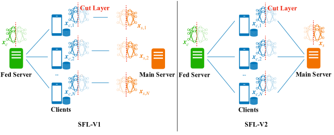
Figure 1: An illustration of SFL framework, and there are two major algorithms, i.e., SFL-V1 (left) and SFL-V2 (right) (Thapa et al., 2022). The global model $\boldsymbol{x}$ is split at the cut layers into two parts: client-side model $\boldsymbol{x}_{c}$ and server-side model $\boldsymbol{x}_{s}$. Each client $n$ trains its own version of client-side model $\boldsymbol{x}_{c,n}$, and the fed server periodically synchronizes all the client-side models. In SFL-V1, the main server maintains one server-side model $\boldsymbol{x}_{s,n}$ for each client $n$, trains and periodically aggregates all server-side models. In SFL-V2, the main server only maintains and trains one server-side model. More discussions on SFL-V1 and SFL-V2 are given in Sec. 2.

Split learning (SL) (Vepakomma et al., 2019) is another distributed approach. By splitting the model across clients and a main server, SL can substantially reduce the computational workload on edge devices. Moreover, recent studies in (Wu et al., 2023; Li & Lyu, 2023) show that SL can outperform FL when data is highly heterogeneous. However, SL’s sequential training among clients can lead to high latency and potential performance loss (caused by catastrophic forgetting), which impedes its practical applicability in real-world distributed systems.

In light of above challenges, (Thapa et al., 2022) proposed split federated learning (SFL) as a hybrid approach that synergizes the strengths of both FL and SL. SFL combines parallel training of FL with partial model training of SL. They proposed two major SFL algorithms: SFL-V1 and SFL-V2. An illustration of these SFL algorithms are shown in Fig. 1. Specifically, the global model (to be trained) is first split at a cut layer into two parts: a client-side model and a server-side model. Then, the clients are responsible for training only the client-side model under the coordination of a fed server (similar to FL). Another server, known as the main server, is responsible for training the server-side model by collaborating with the clients (similar to SL). SFL aims to leverage parallel processing to reduce latency, while also benefiting from the reduced computational workloads and enhanced data heterogeneity handling of SL.

Following (Thapa et al., 2022), there has been an emerging volume of empirical studies on SFL. e.g., (Shiranthika et al., 2023; Shen et al., 2023; Han et al., 2021; Stephanie et al., 2023; Huang et al., 2023b; Waref & Salem, 2022). However, a convergence analysis of SFL is missing in the literature, and this paper aims to provide a comprehensive convergence analysis under different conditions. Convergence theory is crucial for understanding the learning performance of SFL, particularly in the context of heterogeneous data and partial participation scenarios. In practical distributed systems, clients are prone to have different data distributions. Moreover, not all clients may be active or available at all times. These two issues can significantly affect the learning performance of SFL. We aim to provide convergence guarantees for SFL on heterogeneous data (under both full and partial participation). We further compare the results to FL and SL, which provides insights into the practical deployment of various distributed approaches.

1.2 Related Work

Convergence theories of FL and SL. There are many convergence results on FL. Most studies focus on data heterogeneity, e.g., (Wang et al., 2019; Li et al., 2020b; Khaled et al., 2020; Karimireddy et al., 2020; Koloskova et al., 2020). Some studies look at partial participation, e.g., (Yang et al., 2021; Wang & Ji, 2022; Tang & Wong, 2023). There are also convergence results on Mini-Batch SGD, e.g., (Stich, 2019; Woodworth et al., 2020b, a), where (Woodworth et al., 2020b) argued that the key difference between FL and Mini-Batch SGD is the communication frequency.

To our best knowledge, there is only one recent study (Li & Lyu, 2023) discussing the convergence of SFL. The major difference to FL analysis lies in the sequential training manner across clients, while FL clients perform parallel training.

1.3 Challenges and Contributions

Challenges of SFL convergence analysis. When data is homogeneous (IID) across clients, the convergence theory in (Koloskova et al., 2020) (mainly developed for FL) can be applied to SFL. When data is heterogeneous, however, the theory cannot be directly applied due to the client drift problem. The challenge is intensified with clients’ partial participation, which induces bias in the training process. Despite that prior FL theories have handled data heterogeneity (Li et al., 2020b) and partial participation (Wang & Ji, 2022), SFL convergence analysis imposes unique challenges due to the dual-paced model aggregation and model updates at the client-side and server-side. More specifically,

Dual-paced model aggregation in SFL-V1: In SFL-V1, the main server maintains one server-side model for each client, and it periodically aggregates the server-side models. When the main server aggregates its models at the same frequency as the clients, the analysis is the same to that of FL. However, FL analysis cannot be applied when aggregations occur at different frequencies, and it is challenging to analyze the impact of such discrepancy on SFL convergence.

Dual-paced model updates in SFL-V2: In SFL-V2, the main server only maintains one version of server-side model. The clients update the client-side models in a parallel manner while the main server updates the server-side model in a sequential fashion. Hence, each client’s local update depends on the randomness of the previous clients who have interacted with the main server. While (Li & Lyu, 2023) handled sequential client training, their theory cannot be applied to SFL-V2 as they did not consider the aggregation of client-side models. This makes our analysis more challenging than that of FL and SL.

Contributions. We summarize our contributions as follows:

• We provide a convergence analysis of SFL. The analysis is more challenging than prior FL analysis due to the dual-paced model aggregation and model updates. To this end, we derive a key decomposition result (Proposition 3.4) that enables us to analyze the convergence from the server-side and client-side separately.

• Based on the decomposition result, we prove that the convergence guarantees of both SFL-V1 and SFL-V2 are $O(1/T)$ for strongly convex objective and $O(1/\sqrt[3]{T})$ for general convex objective, where $T$ denotes the total number of rounds for SFL training. We further extend the analysis to non-convex objectives and more practical scenarios where some clients may be unavailable during training.

• We conduct simulations on various datasets. We show that the results are consistent with our theories. We further show two surprising results: (i) SFL achieves a better performance when clients maintain a larger portion of the global model; (ii) SFL-V2 outperforms FL and SL when clients have highly heterogeneous data and the number of client is large.

The rest of the paper is organized as follows. Sec. 2 formulates the SFL model. Sec. 3 presents the convergence results for SFL. We conduct numerical experiments in Sec. 4 and conclude in Sec. 5.

2 Problem Formulation

Sec. 2.1 introduces the model. Sec. 2.2 describes the SFL algorithms, and Sec. 2.3 models the client participation.

2.1 Model

We consider a set of clients $\mathcal{N}=\{1,2,\cdots,N\}$, where each client $n\in\mathcal{N}$ has a local private dataset $\mathcal{D}_{n}$ of size $D_{n}=|\mathcal{D}_{n}|$. Suppose the global model parameterized by $\boldsymbol{x}$ has $L$ layers. In SFL, the global model is split at the $L_{c}$-th layer (i.e., the cut layer) into two segments: a client-side model $\boldsymbol{x}_{c}$ (from the first layer to layer $L_{c}$) and a server-side model $\boldsymbol{x}_{s}$ (from layer $L_{c}+1$ to layer $L$), where $\boldsymbol{x}=\left\{\boldsymbol{x}_{c};\boldsymbol{x}_{s}\right\}$. Let $\boldsymbol{x}_{c,n}$ denote the local client-side model of client $n$. The clients train models with the help of two servers: (i) fed server, which periodically aggregates clients’ local models $\boldsymbol{x}_{c,n}$ (similar to FL), and (ii) main server, who trains the server-side model $\boldsymbol{x}_{s}$. In this work, we consider two major SFL algorithms: SFL-V1 and SFL-V2 (Thapa et al., 2022). In SFL-V1, the main server maintains a separate server-side model $\boldsymbol{x}_{s,n}$ corresponding to each client $n$. In comparison, in SFL-V2, the main server only maintains one model $\boldsymbol{x}_{s}$.

Let $F_{n}(\boldsymbol{x};\zeta_{n})$ denote the loss of model $\boldsymbol{x}$ over client $n$’s mini-batch instance $\zeta_{n}$, which is randomly sampled from client $n$’s dataset $\mathcal{D}_{n}$. Let $F_{n}(\boldsymbol{x})\triangleq\mathbb{E}_{\zeta_{n}\sim\mathcal{D}_{n}}[F_{n}(\boldsymbol{x};\zeta_{n})]$ denote the expected loss of model $\boldsymbol{x}$ over client $n$’s dataset. The goal of SFL is to minimize the expected loss of the model $\boldsymbol{x}$ over the datasets of all clients:

$$\min_{\boldsymbol{x}}f(\boldsymbol{x})=\sum_{n=1}^{N}a_{n}F_{n}\left(\boldsymbol{x}\right),$$ (1)

where $a_{n}\in[0,1]$ is the weight of client $n$ satisfying $\sum_{n\in\mathcal{N}}a_{n}=1$. Typically, $a_{n}=D_{n}/\sum_{n^{\prime}\in\mathcal{N}}D_{n^{\prime}}$, where a client with a larger data size is assigned a larger weight (Wu et al., 2023).

2.2 Algorithm Description

We provide a brief description of SFL. Refer to Appendix A for a more detailed discussion. SFL takes a total number of $T$ rounds to solve (1). At the beginning of each round $t$, clients download the recent global client-side model from the fed server, where the model is an aggregated version of the client-side models of the clients from the previous round $t-1$. Each round $t$ contains two stages:

Stage 1: model training. Clients and the main server train the full global model for $\tau$ iterations in each round. In each iteration $i<\tau$, there are three steps:

Step 1: client forward propagation. Each client $n$ samples a mini-batch of data $\zeta_{n}^{t,i}$ from $\mathcal{D}_{n}$, computes the intermediate features (e.g., activation values at the cut layer) over its current model $\boldsymbol{x}_{c,n}^{t,i}$, and sends the activation to the main server. The clients perform forward propagation in parallel.

Step 2: main server training. Upon receiving the activation of each client $n$,

• SFL-V1: the main server computes the loss using the current server-side model $\boldsymbol{x}_{s,n}^{t,i}$. It then computes the gradients over $\boldsymbol{x}_{s,n}^{t,i}$ to update the model. It also computes the gradient over the activation at the cut layer, and sends it to client $n$.

• SFL-V2: the main server computes the loss based on $\boldsymbol{x}_{s}^{t,i}$, based on which it then computes the gradients and updates $\boldsymbol{x}_{s}^{t,i}$. It also computes and sends the gradient over activation at the cut layer to client $n$. Note that the main server sequentially interacts with the clients in a randomized order.

Step 3: client backward propagation. Receiving gradient at the cut layer, each client $n$ computes the client-side gradient using the chain rule, and then updates its model $\boldsymbol{x}_{c,n}^{t,i}$.

Stage 2: model aggregation. Model aggregation can occur for both client-side and server-side models. For the client side, after $\tau$ iterations of model training (i.e., at the end of round $t$), each client sends its current client-side model to the fed server. The fed server aggregates the clients’ models (e.g., weighted averaging), which will be downloaded in the next round $t+1$:

$$\boldsymbol{x}^{t+1}_{c}\leftarrow\sum_{n\in\mathcal{N}}a_{n}\boldsymbol{x}^{t,\tau}_{c,n}.$$ (2)

For the server side, (i) in SFL-V1, after $\tilde{\tau}$ iterations of training, the main server aggregates all server-side models. Note that $\tilde{\tau}$ does not necessarily need to equal $\tau$, but when equality holds, SFL-V1 can be regarded as FL (despite the model splitting). (ii) In SFL-V2, no aggregation occurs since the main server only maintains one model.

2.3 Client Participation

We consider two cases: (i) full participation where all clients are available during training. This can model the scenarios where clients are organizations or companies who likely have sufficient computation and communication resources (Huang et al., 2023a); (ii) partial participation where some clients may be unavailable during training. This can model the cases where clients are edge devices (e.g., mobile phones) that are usually resource-constrained and may be disconnected from the SFL process.

To model partial participation, we use $q_{n}\in[0,1]$ to denote client $n$’s participation level (or probability), and $\boldsymbol{q}=(q_{n},n\in\mathcal{N})$. If $q_{n}=1$, client $n$ participates in every round of SFL with probability one. If $q_{n}<1$, client $n$ is unavailable in some rounds. Denote $\mathcal{P}^{t}(\boldsymbol{q})$ as the set of participating clients in round $t$. In the presence of partial participation, we need to modify (2) (and the potential server-side aggregation) to offset the incurred bias:

$$\boldsymbol{x}^{t+1}_{c}\leftarrow\sum_{n\in\mathcal{P}^{t}(\boldsymbol{q})}\frac{a_{n}}{q_{n}}\boldsymbol{x}^{t,\tau}_{c,n}.$$ (3)

3 Convergence Analysis

We first make technical assumptions in Sec. 3.1. Then, we present a key technical result in Sec. 3.2 to support the SFL convergence analysis. Finally, we provide the convergence results under full participation and partial participation in Sec. 3.3 and Sec. 3.4, respectively.

3.1 Assumptions

We start with some conventional assumptions for convergence analysis in the FL literature.

Assumption 3.1.

($S$-Smoothness) Each client $n$’s loss function $F_{n}$ is $S$-smooth. That is, for all $\boldsymbol{x},\boldsymbol{y}\in\mathbb{R}^{d}$,

$$F_{n}(\boldsymbol{y})\leq F_{n}(\boldsymbol{x})+\langle\nabla F_{n}(\boldsymbol{x}),\boldsymbol{y}-\boldsymbol{x}\rangle+\frac{S}{2}\|\boldsymbol{y}-\boldsymbol{x}\|^{2}.$$ (4)

The smoothness assumption holds for many loss functions in, for example, logistic regression, softmax classifier, and $l_{2}$-norm regularized linear regression (Li et al., 2020b).

Assumption 3.2.

(Unbiased and bounded stochastic gradients with bounded variance) The stochastic gradients $\boldsymbol{g}_{n}(\cdot)$ of $F_{n}\left(\cdot\right)$ are unbiased with the variance bounded by $\sigma_{n}^{2}$:

$$\mathbb{E}_{\zeta_{n}\sim\mathcal{D}_{n}}\left[\boldsymbol{g}_{n}\left(\boldsymbol{x},\zeta_{n}\right)\right]=\nabla F_{n}\left(\boldsymbol{x}\right),$$ (5)

$$\mathbb{E}_{\zeta_{n}\sim\mathcal{D}_{n}}\left[\left\|\boldsymbol{g}_{n}\left(\boldsymbol{x},\zeta_{n}\right)-\nabla F_{n}\left(\boldsymbol{x}\right)\right\|^{2}\right]\leq\sigma_{n}^{2}.$$ (6)

Further, the expected squared norm is bounded by $G^{2}$:

$$\mathbb{E}_{\zeta_{n}\sim\mathcal{D}_{n}}\left\|\boldsymbol{g}_{n}\left(\boldsymbol{x},\zeta_{n}\right)\right\|^{2}\leq G^{2}.$$ (7)

The value of $\sigma_{n}$ measures the level of stochasticity.

Assumption 3.3.

(Heterogeneity) There exists an $\epsilon^{2}$ such that for any client $n$,

$$\left\|\nabla F_{n}\left(\boldsymbol{x}\right)-\nabla f\left(\boldsymbol{x}\right)\right\|^{2}\leq\epsilon^{2}.$$ (8)

A larger $\epsilon^{2}$ indicates a larger degree of data heterogeneity.

3.2 Decomposition

As discussed in Sec. 1.3, analyzing the performance bound of SFL can be more challenging than that of conventional FL counterparts due to the dual-paced model aggregation and model updates. To address this challenge, we decompose the convergence analysis into the server-side and client-side updates, respectively. We give the decomposition below.

Proposition 3.4.

(Convergence decomposition) Let $\boldsymbol{x}^{*}\triangleq[\boldsymbol{x}_{c}^{*};\boldsymbol{x}_{s}^{*}]$ denote the optimal global model that minimizes $f(\cdot)$, and $\boldsymbol{x}^{T}\triangleq[\boldsymbol{x}_{c}^{T};\boldsymbol{x}_{s}^{T}]$ is the global model obtained after $T$ rounds of SFL training. Under Assumption 3.1, we have

$$\mathbb{E}\left[f(\boldsymbol{x}^{T})\right]-f(\boldsymbol{x}^{*})$$ (9)

$$\leq\frac{S}{2}\left(\mathbb{E}||\boldsymbol{x}_{s}^{T}-\boldsymbol{x}_{s}^{*}||^{2}+\mathbb{E}||\boldsymbol{x}_{c}^{T}-\boldsymbol{x}_{c}^{*}||^{2}\right).$$

Proof.

Since $F_{n}$’s are $S$-smooth, it is easy to show that the global loss function $f(\cdot)$ is also $S$-smooth. Thus, we have

$$\mathbb{E}\left[f(\boldsymbol{x}^{T})\right]-f(\boldsymbol{x}^{*})\leq\mathbb{E}\left[\langle\boldsymbol{x}^{T}-\boldsymbol{x}^{*},\nabla f(\boldsymbol{x}^{*})\rangle\right]$$ (10)

$$+\frac{S}{2}\mathbb{E}\left[||\boldsymbol{x}^{T}-\boldsymbol{x}^{*}||^{2}\right]=\frac{S}{2}\mathbb{E}\left[||\boldsymbol{x}^{T}-\boldsymbol{x}^{*}||^{2}\right].$$

Since $\boldsymbol{x}^{T}\triangleq[\boldsymbol{x}_{c}^{T};\boldsymbol{x}_{s}^{T}]$, and $\boldsymbol{x}^{*}\triangleq[\boldsymbol{x}_{c}^{*};\boldsymbol{x}_{s}^{*}]$, we have

$$\mathbb{E}\left[||\boldsymbol{x}^{T}-\boldsymbol{x}^{*}||^{2}\right]$$ (11)

$$= \mathbb{E}\left[||[\boldsymbol{x}_{c}^{T};\boldsymbol{x}_{s}^{T}]-[\boldsymbol{x}_{c}^{*};\boldsymbol{x}_{s}^{*}]||^{2}\right]$$

$$= \mathbb{E}\left[||[\boldsymbol{x}_{c}^{T}-\boldsymbol{x}_{c}^{*};\boldsymbol{x}_{s}^{T}-\boldsymbol{x}_{s}^{*}]||^{2}\right]$$

$$= \mathbb{E}\left[||\boldsymbol{x}_{c}^{T}-\boldsymbol{x}_{c}^{*}||^{2}\right]+\mathbb{E}\left[||\boldsymbol{x}_{s}^{T}-\boldsymbol{x}_{s}^{*}||^{2}\right].$$

Substituting (11) into (10), we complete the proof. ∎

Proposition 3.4 is particularly useful. It shows that despite the challenging dual-paced updates, to bound the SFL performance gap, it suffices to separately bound the gap at the server-side and client-side models. Note that our decomposition can be easily applied to other distributed approaches such as SL. In addition, such a decomposition is not necessarily loose, as our derived bounds for SFL achieve the same order as in FL (see Appendix G.1 for details).

3.3 Results under Full Participation

Built upon Proposition 3.4, we first present the convergence results under full participation. For convenience, define

$$I^{\rm err}\triangleq\left\|\boldsymbol{x}^{0}-\boldsymbol{x}^{\ast}\right\|^{2},\quad\gamma\triangleq 8S/\mu-1,$$ (12)

$$\tau_{\rm min}\triangleq\min\{\tau,\tilde{\tau}\},\quad\tau_{\rm max}\triangleq\max\{\tau,\tilde{\tau}\},$$

and let $\eta^{t}$ represent the learning rate at round $t$. Let $f^{*}$ denotes the optimal global loss, i.e., $f^{*}\triangleq f(\boldsymbol{x}^{*})$. All results are obtained based on Assumptions 3.1-3.3.

 

The convergence results for SFL-V1 and SFL-V2 are summarized in Theorems 3.5 and 3.6, respectively.

Theorem 3.5.

( SFL-V1: full participation)

$\mu$-strongly convex: Let $\eta^{t}\leq\frac{1}{2S\tau_{\rm max}}$,

$$\mathbb{E}\left[f(\boldsymbol{x}^{T})\right]-f^{*}\leq\frac{8SN\sum_{n=1}^{N}a_{n}^{2}\left(2\sigma_{n}^{2}+G^{2}\right)}{\mu^{2}\left(\gamma+T\right)}$$ (13)

$$+\frac{768S^{2}\ \sum_{n=1}^{N}a_{n}\left(2\sigma_{n}^{2}+G^{2}\right)}{\mu^{3}\left(\gamma+T\right)\left(\gamma+1\right)}+\frac{S(\gamma+1)I^{\rm err}}{2(\gamma+T)}.$$

General convex: Let $\eta^{t}\leq\frac{1}{2S\tau_{\rm max}}$,

$$\mathbb{E}\left[f\left(\boldsymbol{x}^{T}\right)\right]-f^{*}\leq\frac{SI^{\rm err}}{2(T+1)}$$ (14)

$$+\frac{1}{2}\left(\frac{(\tilde{\tau}^{2}+\tau^{2})I^{\rm err}N}{\tau_{\min}^{2}(T+1)}\sum_{n=1}^{N}a_{n}^{2}\left(2\sigma_{n}^{2}+G^{2}\right)\right)^{\frac{1}{2}}$$

$$+\frac{1}{2}\left(\frac{24(\tilde{\tau}^{2}+\tau^{2})SI^{\rm err}}{\tau_{\min}^{2}(T+1)}\sum_{n=1}^{N}a_{n}\left(2\sigma_{n}^{2}+G^{2}\right)\right)^{\frac{1}{3}}.$$

Non-convex: Let $\eta^{t}\leq\min\left\{\frac{1}{16S\tau_{\max}},\frac{\tau_{\min}}{8SN\tau_{\max}^{2}\sum_{n=1}^{N}a_{n}^{2}}\right\}$,

$$\frac{1}{T}\sum_{t=0}^{T-1}\eta^{t}\mathbb{E}\left[\left\|\nabla_{\boldsymbol{x}}f\left(\boldsymbol{x}^{t}\right)\right\|^{2}\right]\leq\frac{4}{T\tau_{\min}}\left(f\left(\boldsymbol{x}^{0}\right)-f^{\ast}\right)$$ (15)

$$+\frac{8NS(\tau^{2}+\tilde{\tau}^{2})}{T\tau_{\rm min}}\sum_{n=1}^{N}a_{n}^{2}\left(\sigma_{n}^{2}+\epsilon^{2}\right)\sum_{t=0}^{T-1}\left(\eta^{t}\right)^{2}.$$

Theorem 3.6.

( SFL-V2: full participation)

$\mu$-strongly convex: Let $\eta^{t}\leq\frac{1}{2S\tau}$,

$$\mathbb{E}\left[f(\boldsymbol{x}^{T})\right]-f^{*}\leq\frac{8SN\sum_{n=1}^{N}(a_{n}^{2}+1)\left(2\sigma_{n}^{2}+G^{2}\right)}{\mu^{2}\left(\gamma+T\right)}$$ (16)

$$+\frac{768S^{2}\ \sum_{n=1}^{N}(a_{n}+1)\left(2\sigma_{n}^{2}+G^{2}\right)}{\mu^{3}\left(\gamma+T\right)\left(\gamma+1\right)}+\frac{S(\gamma+1)I^{\rm err}}{2(\gamma+T)}.$$

General convex: Let $\eta^{t}\leq\frac{1}{2S\tau}$,

$$\mathbb{E}\left[f\left(\boldsymbol{x}^{T}\right)\right]-f^{*}\leq\frac{SI^{\rm err}}{2(T+1)}$$ (17)

$$+\frac{1}{2}\left(\frac{NI^{\rm err}}{T+1}\sum_{n=1}^{N}(a_{n}^{2}+1)\left(2\sigma_{n}^{2}+G^{2}\right)\right)^{\frac{1}{2}}$$

$$+\frac{1}{2}\left(\frac{24SI^{\rm err}}{T+1}\sum_{n=1}^{N}(a_{n}+1)\left(2\sigma_{n}^{2}+G^{2}\right)\right)^{\frac{1}{3}}.$$

Non-convex: Let $\eta^{t}\leq\min\left\{\frac{1}{16S\tau},\frac{1}{8SN^{2}\tau}\right\}$,

$$\frac{1}{T}\sum_{t=0}^{T-1}\eta^{t}\mathbb{E}\left[\left\|\nabla_{\boldsymbol{x}}f\left(\boldsymbol{x}^{t}\right)\right\|^{2}\right]\leq\frac{4}{T\tau}\left(f\left(\boldsymbol{x}^{0}\right)-f^{\ast}\right)$$ (18)

$$+\frac{8NS\tau}{T}\sum_{n=1}^{N}(a_{n}^{2}+1)\left(\sigma_{n}^{2}+\epsilon^{2}\right)\sum_{t=0}^{T-1}\left(\eta^{t}\right)^{2}.$$

Proofs of Theorems 3.5-3.6 are given in Appendices C-D, respectively. We summarize the key findings below.

Convergence rate. The convergence bounds of both SFL-V1 and SFL-V2 achieve an order of $O(1/T)$ on strongly convex (and non-convex) objectives. For general convex objectives, the convergence rate becomes $O(1/\sqrt[3]{T})$. Note that our bounds match the existing bounds for FL and SL (in terms of the order of $T$) on heterogeneous data for strongly convex objectives. For a more detailed comparison, please refer to Appendix G.1.

Impact of data heterogeneity. The convergence bounds increase as the level of data heterogeneity increases. For example, in (15), the bound increases in $\epsilon^{2}$ (see Assumption 3.3). This means that SFL tends to perform worse when clients’ data are more heterogeneous, which is a commonly observed phenomenon in distributed learning, e.g., FL.

Choice of learning rate. One should use a smaller learning rate when the number of local iteration $\tau$ increases. This bears a similar spirit to (Li et al., 2020b). In addition, our results indicate that a proper choice of constant learning rate suffices for SFL convergence. It would be an interesting direction to investigate whether diminishing learning rates are able to achieve faster convergence.

Comparison between SFL-V1 and SFL-V2. The convergence results between the two SFL versions are very similar, except that $a_{n}^{2}$ (and $a_{n}$) in SFL-V1 are replaced by $a_{n}^{2}+1$ (and $a_{n}+1$) in SFL-V2. See (13) and (16) for an inspection. We will show in Sec. 4 that SFL-V1 and SFL-V2 achieve similar accuracy (except under highly heterogeneous data).

3.4 Results under Partial Participation

Now, we present the results under partial participation.

Theorem 3.7.

( SFL-V1: partial participation)

$\mu$-strongly convex: Let $\eta^{t}\leq\frac{1}{2S\tau_{\rm max}}$,

$$\mathbb{E}\left[f(\boldsymbol{x}^{T})\right]-f^{*}\leq\frac{8SN\sum_{n=1}^{N}a_{n}^{2}\left(2\sigma_{n}^{2}+G^{2}+\frac{G^{2}}{q_{n}}\right)}{\mu^{2}\left(\gamma+T\right)}$$ (19)

$$+\frac{768S^{2}\ \sum_{n=1}^{N}a_{n}\left(2\sigma_{n}^{2}+G^{2}\right)}{\mu^{3}\left(\gamma+T\right)\left(\gamma+1\right)}+\frac{S(\gamma+1)I^{\rm err}}{2(\gamma+T)}.$$

General convex: Let $\eta^{t}\leq\frac{1}{2S\tau_{\rm max}}$,

$$\mathbb{E}\left[f\left(\boldsymbol{x}^{T}\right)\right]-f^{*}\leq\frac{SI^{\rm err}}{2(T+1)}$$ (20)

$$+\frac{1}{2}\left(\frac{(\tilde{\tau}^{2}+\tau^{2})I^{\rm err}N}{\tau_{\min}^{2}(T+1)}\sum_{n=1}^{N}a_{n}^{2}\left(2\sigma_{n}^{2}+G^{2}+\frac{G^{2}}{q_{n}}\right)\right)^{\frac{1}{2}}$$

$$+\frac{1}{2}\left(\frac{24(\tilde{\tau}^{2}+\tau^{2})SI^{\rm err}}{\tau_{\min}^{2}(T+1)}\sum_{n=1}^{N}a_{n}\left(2\sigma_{n}^{2}+G^{2}\right)\right)^{\frac{1}{3}}.$$

Non-convex: Let $\eta^{t}\leq\min\{\frac{1}{16S\tau_{\max}},\frac{\tau_{\min}}{8SN\tau_{\max}^{2}\sum_{n=1}^{N}\frac{a_{n}^{2}}{q_{n}}}\}$,

$$\frac{1}{T}\sum_{t=0}^{T-1}\eta^{t}\mathbb{E}\left[\left\|\nabla_{\boldsymbol{x}}f\left(\boldsymbol{x}^{t}\right)\right\|^{2}\right]\leq\frac{4}{T\tau_{\min}}\left(f\left(\boldsymbol{x}^{0}\right)-f^{\ast}\right)$$ (21)

$$+\frac{8NS(\tau^{2}+\tilde{\tau}^{2})}{T\tau_{\min}}\sum_{n=1}^{N}\frac{a_{n}^{2}}{q_{n}}\left(\sigma_{n}^{2}+\epsilon^{2}\right)\sum_{t=0}^{T-1}\left(\eta^{t}\right)^{2}.$$

Theorem 3.8.

( SFL-V2: partial participation)

$\mu$-strongly convex: Let $\eta^{t}\leq\frac{1}{2S\tau}$,

$$\mathbb{E}\left[f\left(\boldsymbol{x}^{T}\right)\right]-f^{*}\leq$$ (22)

$$\frac{8SN\sum_{n=1}^{N}(a_{n}^{2}+1)\left(2\sigma_{n}^{2}+G^{2}+\frac{G^{2}}{q_{n}}\right)}{\mu^{2}\left(\gamma+T\right)}$$

$$+\frac{768S^{2}\ \sum_{n=1}^{N}(a_{n}+1)\left(2\sigma_{n}^{2}+G^{2}\right)}{\mu^{3}\left(\gamma+T\right)\left(\gamma+1\right)}+\frac{S(\gamma+1)I^{\rm err}}{2(\gamma+T)}.$$

General convex: Let $\eta^{t}\leq\frac{1}{2S\tau}$,

$$\mathbb{E}\left[f\left(\boldsymbol{x}^{T}\right)\right]-f^{*}\leq\frac{SI^{\rm err}}{2(T+1)}$$ (23)

$$+\frac{1}{2}\left(\frac{NI^{\rm err}}{T+1}\sum_{n=1}^{N}(a_{n}^{2}+1)\left(2\sigma_{n}^{2}+G^{2}+\frac{G_{n}^{2}}{q_{n}}\right)\right)^{\frac{1}{2}}$$

$$+\frac{1}{2}\left(\frac{24SI^{\rm err}}{T+1}\sum_{n=1}^{N}(a_{n}+1)\left(2\sigma_{n}^{2}+G^{2}\right)\right)^{\frac{1}{3}}.$$

Non-convex: Let $\eta^{t}\leq\min\left\{\frac{1}{16S\tau},\frac{1}{8SN^{2}\tau\sum_{n=1}^{N}\frac{a_{n}^{2}}{q_{n}}}\right\}$,

$$\frac{1}{T}\sum_{t=0}^{T-1}\eta^{t}\mathbb{E}\left[\left\|\nabla_{\boldsymbol{x}}f\left(\boldsymbol{x}^{t}\right)\right\|^{2}\right]\leq\frac{4}{T\tau}\left(f\left(\boldsymbol{x}_{0}\right)-f^{\ast}\right)$$ (24)

$$+\frac{8NS\tau}{T}\sum_{n=1}^{N}\frac{a_{n}^{2}+1}{q_{n}}\left(\sigma_{n}^{2}+\epsilon^{2}\right)\sum_{t=0}^{T-1}\left(\eta^{t}\right)^{2}.$$

The proofs are given in Appendices E-F.

Impact of partial participation. In practical cross-device settings, some clients may not participate in all rounds of training, i.e., $q_{n}<1$ for some $n$. This brings an additional term $G^{2}/q_{n}$ to the convergence bound (e.g., see (14) and (20)), meaning that partial participation worsens SFL performance. This is also observed in FL literature (e.g., (Wang & Ji, 2022)) and is consistent with our numerical results.

4 Numerical Results

4.1 Experiment setup

We conduct experiments on CIFAR-10 and CIFAR-100 (Krizhevsky, 2009). Both datasets consist of 60k images (50k for training and 10k for testing), except that CIFAR-10 has 10 classes while CIFAR-100 has 100 classes. We use cross-entropy as the loss function. To simulate data heterogeneity, we adopt the widely used Dirichlet distribution (Hsu et al., 2019) with a controlling parameter $\beta$. Here, a smaller $\beta$ corresponds to a higher level of data heterogeneity across clients. We use ResNet-18 as the model structure and consider four types of model splitting represented by $L_{c}=\{1,2,3,4\}$, where $L_{c}=n$ means the model is split after the $n$-th residual block. We consider two major distributed approaches as the benchmark, i.e., FL (in particular FedAvg (McMahan et al., 2017)) and SL (Vepakomma et al., 2019). The learning rates for SFL-V1, SFL-V2, FL and SL are set as $0.01$. The batch-size $b_{s}$ is 128, and we run experiments for $T=200$ rounds. Unless stated otherwise, we use $N=10,\beta=0.1,E=5$, where $E$ is the local epoch number, and hence $\tau=\lceil\frac{D_{n}}{b_{s}}\rceil\times E$. Our codes are provided in the supplementary material.

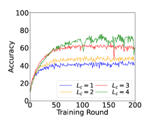
((a))

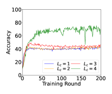
((b))

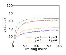
((c))

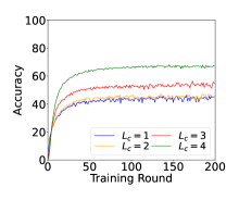
((d))

Figure 2: Impact of the choice of cut layer on SFL performance.

4.2 Impact of system parameters on SFL performance

Impact of cut layer. We first investigate how the choice of the cut layer $L_{c}$ affects the SFL performance. The results are reported in Fig. 2. We observe that for both SFL-V1 and SFL-V2, the performance increases in $L_{c}$ (i.e., clients have a larger proportion of the global model). We think this is associated with our empirical observation that the average client gradient variance gets smaller with $L_{c}$. Intuitively, a smaller gradient variance implies a lower degree of the client drift issue, which leads to a better algorithm performance. Based on this observation, we use $L_{c}=4$ for SFL (and SL) for the following experiments.

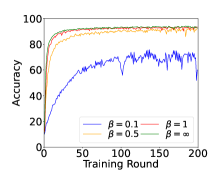
((a))

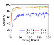
((b))

((c))

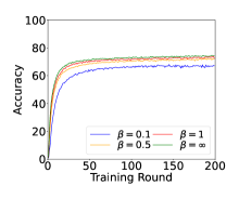
((d))

Figure 3: Impact of data heterogeneity on SFL performance.

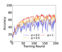
((a))

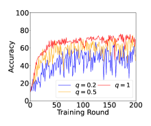
((b))

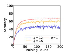
((c))

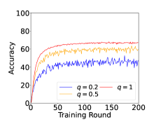
((d))

Figure 4: Impact of client participation on SFL performance.

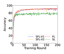
((a))

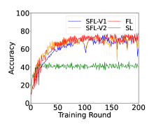
((b))

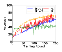
((c))

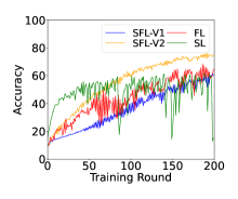
((d))

Figure 5: Performance comparison on CIFAR-10.

Impact of data heterogeneity. We study the impact of data heterogeneity on SFL performance, where we use $\beta\in\{0.1,0.5,1,\infty\}$, and $\beta=\infty$ means clients have IID data. The results are reported in Fig. 3. We observe that a higher level of data heterogeneity (i.e., a smaller $\beta$) leads to slower algorithm convergence and a lower accuracy for both SFL-V1 and SFL-V2. The observation is consistent with our convergence bound, e.g., in (18), the performance bound increases in $\epsilon^{2}$. Note that the negative impact of heterogeneity is commonly observed in distributed learning literature including FL (Huang et al., 2023a) and SL (Shen et al., 2023).

Impact of partial participation. We study the impact of client participation and let $q_{n}=q\in\{0.2,0.5,1\},\forall n.$ The results are reported in Fig. 4. We observe that a lower level of participation leads to less stable convergence and also a smaller accuracy. This is consistent with our convergence results, e.g., in (22), the bound decreases in clients’ participation level $q_{n}$. Partial participation is expected in practical cross-device scenarios where clients are resourced-constrained edge devices. It is important to develop efficient algorithms as well as effective incentive mechanisms to encourage clients’ participation in SFL.

4.3 Comparison among SFL, FL, and SL.

We now compare SFL to FL and SL. We consider different combinations of data heterogeneity $\beta\in\{0.1,0.5\}$ and cohort sizes $N\in\{10,50,100\}$. The results are reported in Fig. 5. When data is mildly heterogeneous (i.e., $\beta=0.5$), SFL and FL have similar convergence rates and accuracy performance. Note that SL seems to under-perform SFL and FL. We think this is mainly due to the catastrophic forgetting issue, which has been observed in (Shen et al., 2023; Gao et al., 2020).

SFL outperforms FL and SL under highly heterogeneous data and a large client number. When data becomes more non-IID (i.e., $\beta=0.1$), SFL-V2 tends to outperform FL and SL. The improvement becomes more significant as the cohort size gets larger. The client drift issue faced by FL becomes severer when the cohort size and data heterogeneity increase. However, SFL can help mitigate the client drift issue by splitting the model and offloading the training to the main server, leading to a better performance than FL. This observation also indicates that SFL-V2 can be a more appealing solution than FL for practical cross-device systems, as it achieves a better performance while requiring smaller computation overheads from edge devices.

Additional experiments. In Appendix H, we further investigate how the epoch number affects the SFL performance. In addition, since the results in the main paper are based on the accuracy metric, we additionally show the results using the loss metric and observed similar (but opposite) trends. That is, a higher accuracy is associated with a smaller loss.

5 Conclusion

In this work, we provided the first comprehensive convergence analysis of SFL for strongly convex, general-convex, and non-convex objectives on heterogeneous data. One key challenge is the dual-paced model updates. We get around this issue by decomposing the performance gap of the global model into the client-side and server-side gaps. We further extend our analysis to the more practical scenario with partial client participation. Numerical experiments validate our theories and further show that SFL can outperform FL and SL under highly heterogeneous data and a large client number.

For future work, we can apply our derived bounds to optimize SFL system performance, considering model accuracy, communication overhead, and computational workload of clients. It is also interesting to theoretically analyze how the choice of the cut layer affects the SFL performance.

Impact Statements

The goal of this work is to provide a comprehensive analysis on the convergence of SFL. Our theoretical results have two potential impacts. First, we provide a thorough understanding on the performance of SFL, which potentially guides the implementation of SFL (e.g., the choice between FL and SFL, the choice of hyper-parameters and cut layers). Second, the convergence results can be used for modeling the training performance of SFL. Together with an effective modeling of communication and computation overheads of clients, researchers will be able to perform SFL system optimization. Due to the reduced clients’ training loads in SFL, such a system optimization can potentially minimize the burden at clients (e.g., human mobile devices) while maintaining client privacy and satisfactory training performance.

We organize the entire appendix file as follows:

In Sec. A, we provide detailed algorithmic descriptions.

In Sec. B, we provide notations and some technical lemmas.

• In Sec. B.1, we provide some notations

• In Sec. B.2, we recall SFL-V1 and SFL-V2

• In Sec. B.3, we recall the assumptions

• In Sec. B.4, we provide some useful technical lemmas together with their proofs

In Sec. C, we prove Theorem 3.5, i.e., convergence of SFL-V1 under full participation.

• In Sec. C.1, we prove the strongly convex case

• In Sec. C.2, we prove the general convex case

• In Sec. C.3, we prove the non-convex case

In Sec. D, we prove Theorem 3.6, i.e., convergence of SFL-V2 under full participation.

• In Sec. D.1, we prove the strongly convex case

• In Sec. D.2, we prove the general convex case

• In Sec. D.3, we prove the non-convex case

In Sec. E, we prove Theorem 3.7, i.e., convergence of SFL-V1 under partial participation.

• In Sec. E.1, we prove the strongly convex case

• In Sec. E.2, we prove the general convex case

• In Sec. E.3, we prove the non-convex case

In Sec. F, we prove Theorem 3.8, i.e., convergence of SFL-V2 under partial participation.

• In Sec. F.1, we prove the strongly convex case

• In Sec. F.2, we prove the general convex case

• In Sec. F.3, we prove the non-convex case

In Sec. G, we SFL to other distributed approaches, i.e., FL, SL, and Mini-Batch SGD.

• In Sec. G.1, we compare their convergence bounds

• In Sec. G.2, we compare their overheads in terms of communication and computation

In Sec. H, we provide more experimental results.

Appendix A Algorithm description

For version 1, the client-side model parameter and M-server-side model parameter are aggregated every $\tau$ and $\tilde{\tau}$ iterations, respectively. In iteration $i$ of round $t$, each client $n$ samples a mini-batch of data $\zeta_{n}^{t,i}$ from $\mathcal{D}_{n}$, computes the intermediate features $h(\boldsymbol{x}_{c,n}^{t,i};\zeta_{n}^{t,i})$ (e.g., activation values at the cut layer) over its current model $\boldsymbol{x}_{c,n}^{t,i}$, and sends $h(\boldsymbol{x}_{c,n}^{t,i};\zeta_{n}^{t,i})$ to the M-server. For each client $n$, the M-server computes the loss $F_{n}(h(\boldsymbol{x}_{c,n}^{t,i};\zeta_{n}^{t,i}),\boldsymbol{x}_{s,n}^{t,i})$ based on $\boldsymbol{x}_{s,n}^{t,i}$. Let $\nabla$ denote a gradient operator and $\nabla_{\boldsymbol{w}}F$ represents the gradient of $F$ w.r.t. $\boldsymbol{w}$. The M-server computes the M-server-side gradient $\boldsymbol{g}_{s,n}^{t,i}(\boldsymbol{x}_{s,n}^{t,i};\zeta_{n}^{t,i})=\nabla_{\boldsymbol{x}_{s}}F_{n}(h(\boldsymbol{x}_{c,n}^{t,i};\zeta_{n}^{t,i}),\boldsymbol{x}_{s,n}^{t,i})$, the gradient over the intermediate features (activations) at the cut layer $\boldsymbol{r}_{c,n}^{t,i}(\boldsymbol{x}^{t,i}_{s,n};\zeta_{n}^{t,i})=\nabla_{h}F_{n}(h(\boldsymbol{x}_{c,n}^{t,i};\zeta_{n}^{t,i}),\boldsymbol{x}_{s,n}^{t,i})$, and sends $\boldsymbol{r}_{c,n}^{t,i}(\boldsymbol{x}^{t,i}_{s,n};\zeta_{n}^{t,i})$ to client $n$. Each client $n$ computes the client-side gradient $\boldsymbol{g}_{c,n}^{t,i}(\boldsymbol{x}^{t,i}_{c,n};\zeta_{n}^{t,i})$ based on $\boldsymbol{r}_{c,n}^{t,i}(\boldsymbol{x}^{t,i}_{s,n};\zeta_{n}^{t,i})$ using the chain rule.

For version 2, the client-side model is aggregated every $\tau$ iterations, while the M-server trains only one version of the M-server-side model.

Algorithm 1 SFL-V1

Input: $\tau,\tilde{\tau},T$, and learning rate $\eta_{t}$

Output: Global model $\boldsymbol{x}^{T}=\{\boldsymbol{x}_{c}^{T},\boldsymbol{x}_{s}^{T}\}$

Initialize $\boldsymbol{x}^{0}=\{\boldsymbol{x}_{c}^{0},\boldsymbol{x}_{s}^{0}\}$;

for $i=0,\ldots,(T-1)\tau_{\max}$ do

       Determine participating client set $\mathcal{P}^{t}\subseteq\mathcal{N}$; Phase 1: model training. each client $n\in\mathcal{P}^{t}$:  

2             Sample a mini-batch $\zeta_{n}^{t,i}$; Send $h(\boldsymbol{x}_{c,n}^{t,i};\zeta_{n}^{t,i})$ to the M-server; the M-server:  

3                   Compute $F_{n}(h(\boldsymbol{x}_{c,n}^{t,i};\zeta_{n}^{t,i}),\boldsymbol{x}_{s}^{t,i})$, $\boldsymbol{g}_{s,n}^{t,i}(\boldsymbol{x}_{s,n}^{t,i};\zeta_{n}^{t,i})$, and $\boldsymbol{r}_{c,n}^{t,i}(\boldsymbol{x}^{t,i}_{s,n};\zeta_{n}^{t,i})$; Send $\boldsymbol{r}_{c,n}^{t,i}(\boldsymbol{x}^{t,i}_{s,n};\zeta_{n}^{t,i})$ to client $n\in\mathcal{P}^{t}$; $\boldsymbol{x}_{s,n}^{t,i+1}\leftarrow\boldsymbol{x}_{s,n}^{t,i}-\eta_{t}\boldsymbol{g}_{s,n}^{t,i}(\boldsymbol{x}_{s,n}^{t,i};\zeta_{n}^{t,i})$;

4            Compute $\boldsymbol{g}_{c,n}^{t,i}(\boldsymbol{x}_{c,n}^{t,i};\zeta_{n}^{t,i})$; $\boldsymbol{x}_{c,n}^{t,i+1}\leftarrow\boldsymbol{x}_{c,n}^{t,i}-\eta_{t}\boldsymbol{g}_{c,n}^{t,i}(\boldsymbol{x}_{c,n}^{t,i};\zeta_{n}^{t,i})$;

       Phase 2: model aggregation. if $i\%\tau=0$ then

5             each client $n\in\mathcal{P}^{t}$:  

6                   Send $\boldsymbol{x}_{c,n}^{t,\tau}$ to the F-server;

7            the F-server:  

8                   $\boldsymbol{x}_{c}^{t+1}\leftarrow\sum_{n\in\mathcal{P}^{t}}a_{n}\boldsymbol{x}_{c,n}^{t,\tau}$;

9            each client $n\in\mathcal{N}$:  

10                   $\boldsymbol{x}_{c,n}^{t,0}\leftarrow\boldsymbol{x}_{c}^{t}$;

11            

12      if $i\%\tilde{\tau}=0$ then

13             the M-server:  

14                   $\boldsymbol{x}_{s}^{t+1}\leftarrow\sum_{n\in\mathcal{P}^{t}}a_{n}\boldsymbol{x}_{s,n}^{t,\tilde{\tau}}$. $\boldsymbol{x}_{s,n}^{t,0}\leftarrow\boldsymbol{x}_{s}^{t},\forall n\in\mathcal{N}$;

15            

16      

Algorithm 2 SFL-V2

Input: $\tau,T$, and learning rate $\eta_{t}$

Output: Global model $\boldsymbol{x}^{T}=\{\boldsymbol{x}_{c}^{T},\boldsymbol{x}_{s}^{T}\}$

Initialize $\boldsymbol{x}^{0}=\{\boldsymbol{x}_{c}^{0},\boldsymbol{x}_{s}^{0}\}$;

for $t=0,\ldots,T-1$ do

       Determine participating client set $\mathcal{P}^{t}\subseteq\mathcal{N}$; Phase 1: model training. each client $n\in\mathcal{P}^{t}$:  

18             $\boldsymbol{x}_{c,n}^{t,0}\leftarrow\boldsymbol{x}_{c}^{t}$; for $i=0,\ldots,\tau-1$ do

19                   Sample a mini-batch $\zeta_{n}^{t,i}$; Send $h(\boldsymbol{x}_{c,n}^{t,i};\zeta_{n}^{t,i})$ to the M-server; the M-server:  

20                         Compute $F_{n}(h(\boldsymbol{x}_{c,n}^{t,i};\zeta_{n}^{t,i}),\boldsymbol{x}_{s}^{t,i})$, $\boldsymbol{g}_{s,n}^{t,i}(\boldsymbol{x}_{s}^{t,i};\zeta_{n}^{t,i})$, and $\boldsymbol{r}_{c,n}^{t,i}(\boldsymbol{x}^{t,i}_{s};\zeta_{n}^{t,i})$; Send $\boldsymbol{r}_{c,n}^{t,i}(\boldsymbol{x}^{t,i}_{s};\zeta_{n}^{t,i})$ to client $n\in\mathcal{P}^{t}$; $\boldsymbol{x}_{s}^{t,i+1}\leftarrow\boldsymbol{x}_{s}^{t,i}-\eta_{t}\boldsymbol{g}_{s,n}^{t,i}(\boldsymbol{x}_{s}^{t,i};\zeta_{n}^{t,i})$;

21                  Compute $\boldsymbol{g}_{c,n}^{t,i}(\boldsymbol{x}_{c,n}^{t,i};\zeta_{n}^{t,i})$; $\boldsymbol{x}_{c,n}^{t,i+1}\leftarrow\boldsymbol{x}_{c,n}^{t,i}-\eta_{t}\boldsymbol{g}_{c,n}^{t,i}(\boldsymbol{x}_{c,n}^{t,i};\zeta_{n}^{t,i})$;

22            

23      the M-server:  

24             $\boldsymbol{x}_{s}^{t+1,0}\leftarrow\boldsymbol{x}_{s}^{t,\tau}$;

       Phase 2: model aggregation. each client $n\in\mathcal{P}^{t}$:  

25             Send $\boldsymbol{x}_{c,n}^{t,\tau}$ to the F-server;

26      the F-server:  

27             $\boldsymbol{x}_{c}^{t+1}\leftarrow\sum_{n\in\mathcal{P}^{t}}a_{n}\boldsymbol{x}_{c,n}^{t,\tau}$.

28      

Appendix B Notations and technical lemmas

B.1 Notations

Recall that the objective of SFL is given by

$$\min_{\boldsymbol{x}}f(\boldsymbol{x}):=\sum_{n=1}^{N}a_{n}F_{n}(\boldsymbol{x})$$ (25)

We define

• $\boldsymbol{x}_{c}$ and $\boldsymbol{x}_{s}$: global model parameter on the clients and server sides, respectively.

• $\boldsymbol{x}_{c,n}$ and $\boldsymbol{x}_{s,n}$: local forms of parameter on client $n$ and on the main server corresponding to client $n$ (in SFL-V1).

• $\nabla F_{c,n}\left(\cdot\right)$ and $\nabla F_{s,n}\left(\cdot\right)$: the gradients of $F_{n}\left(\cdot\right)$ over $\boldsymbol{x}_{c}$ and $\boldsymbol{x}_{s}$, respectively.

• $\boldsymbol{g}_{c,n}\left(\cdot\right)$ and $\boldsymbol{g}_{s,n}\left(\cdot\right)$: the stochastic gradients of $F_{n}\left(\cdot\right)$ over $\boldsymbol{x}_{c}$ and $\boldsymbol{x}_{s}$, respectively.

For convenience, we omit the notation for mini-batch training data when referring to stochastic gradients.

Further, we recall how SFL-V1 and SFL-V2 update models below.

B.2 SFL-V1 and SFL-V2 model updates

Let $q_{n}$ denote the participating probability of client $n$ and define $\boldsymbol{q}:=\left\{q_{1},\ldots,q_{N}\right\}$. We denote $\mathbf{I}_{n}^{t}$ as a binary variable, taking 1 if client $n$ participates in model training in round $t$, and 0 otherwise. $\mathbf{I}_{n}^{t}$ follows a Bernoulli distribution with an expectation of $q_{n}$. Denote $\mathcal{P}^{t}\left(\boldsymbol{q}\right)$ as the set of participating clients in round $t$.

Parameter update for SFL-V1:

• Local training of client $n$: $\boldsymbol{x}^{t,0}_{c,n}\leftarrow\boldsymbol{x}^{t}_{c}$, $\boldsymbol{x}^{t,i+1}_{c,n}\leftarrow\boldsymbol{x}^{t,i}_{c,n}-\eta^{t}\boldsymbol{g}_{c,n}^{t,i}\left(\boldsymbol{x}^{t,i}_{c,n}\right)$, $\boldsymbol{x}^{t+1}_{c,n}\leftarrow\boldsymbol{x}^{t,\tau}_{c,n}$;

• Client-side global aggregation:

  • Full participation: ${\boldsymbol{x}}^{t+1}_{c}\leftarrow\boldsymbol{x}^{t}_{c}-\eta^{t}\sum_{n\in\mathcal{N}}a_{n}\sum_{i=0}^{\tau}{\boldsymbol{g}}_{c,n}^{t,i}\left(\boldsymbol{x}^{t,i}_{c,n}\right)$;

  • Partial participation: ${\boldsymbol{x}}^{t+1}_{c}\leftarrow\boldsymbol{x}^{t}_{c}-\eta^{t}\sum_{n\in\mathcal{P}^{t}\left(\boldsymbol{q}\right)}\frac{a_{n}}{q_{n}}\sum_{i=0}^{\tau}{\boldsymbol{g}}_{c,n}^{t,i}\left(\boldsymbol{x}^{t,i}_{c,n}\right)$;

• M-server-side model update:

  • Full participation: $\boldsymbol{x}^{t+1}_{s}\leftarrow\boldsymbol{x}^{t}_{s}-\eta^{t}\sum_{n\in\mathcal{N}}a_{n}\sum_{i=0}^{\tilde{\tau}-1}\boldsymbol{g}_{s,n}^{t,i}\left(\boldsymbol{x}^{t,i}_{s,n}\right)$;

  • Partial participation: $\boldsymbol{x}^{t+1}_{s}\leftarrow\boldsymbol{x}^{t}_{s}-\eta^{t}\sum_{n\in\mathcal{P}^{t}\left(\boldsymbol{q}\right)}\frac{a_{n}}{q_{n}}\sum_{i=0}^{\tilde{\tau}-1}\boldsymbol{g}_{s,n}^{t,i}\left(\boldsymbol{x}^{t,i}_{s,n}\right)$.

Parameter update for SFL-V2:

• Local training of client $n$: $\boldsymbol{x}^{t,0}_{c,n}\leftarrow\boldsymbol{x}^{t}_{c}$, $\boldsymbol{x}^{t,i+1}_{c,n}\leftarrow\boldsymbol{x}^{t,i}_{c,n}-\eta^{t}\boldsymbol{g}_{c,n}^{t,i}\left(\boldsymbol{x}^{t,i}_{c,n}\right)$, $\boldsymbol{x}^{t+1}_{c,n}\leftarrow\boldsymbol{x}^{t,\tau}_{c,n}$;

• Client-side global aggregation:

  • Full participation: ${\boldsymbol{x}}^{t+1}_{c}\leftarrow\boldsymbol{x}^{t}_{c}-\eta^{t}\sum_{n\in\mathcal{N}}a_{n}\sum_{i=0}^{\tau}{\boldsymbol{g}}_{c,n}^{t,i}\left(\boldsymbol{x}^{t,i}_{c,n}\right)$;

  • Partial participation: ${\boldsymbol{x}}^{t+1}_{c}\leftarrow\boldsymbol{x}^{t}_{c}-\eta^{t}\sum_{n\in\mathcal{P}^{t}\left(\boldsymbol{q}\right)}\frac{a_{n}}{q_{n}}\sum_{i=0}^{\tau}{\boldsymbol{g}}_{c,n}^{t,i}\left(\boldsymbol{x}^{t,i}_{c,n}\right)$;

• M-server-side model update:

  • Full participation: $\boldsymbol{x}^{t+1}_{s}\leftarrow\boldsymbol{x}^{t}_{s}-\eta^{t}\sum_{n\in\mathcal{N}}\sum_{i=0}^{\tau-1}\boldsymbol{g}_{s,n}^{t,i}\left(\boldsymbol{x}^{t,i}_{s,n}\right)$;

  • Partial participation: $\boldsymbol{x}^{t+1}_{s}\leftarrow\boldsymbol{x}^{t}_{s}-\eta^{t}\sum_{n\in\mathcal{P}^{t}\left(\boldsymbol{q}\right)}\frac{1}{q_{n}}\sum_{i=0}^{\tau-1}\boldsymbol{g}_{s,n}^{t,i}\left(\boldsymbol{x}^{t,i}_{s,n}\right)$.

B.3 Assumptions

We further recall the following assumptions for clients’ loss functions in the proof.

Assumption B.1.

For each client $n\in\mathcal{N}$:

• The loss $F_{n}\left(\cdot\right)$ is $S$-smooth:

  $$\left\|\nabla F_{n}\left(\boldsymbol{x}\right)-\nabla F_{n}\left(\boldsymbol{y}\right)\right\|\leq S\left\|\boldsymbol{x}-\boldsymbol{y}\right\|,\forall\boldsymbol{x},\boldsymbol{y},$$ (26)

  $$F_{n}(\boldsymbol{y})\leq F_{n}(\boldsymbol{x})+\langle\nabla F_{n}(\boldsymbol{x}),\boldsymbol{y}-\boldsymbol{x}\rangle+\frac{S}{2}\|\boldsymbol{y}-\boldsymbol{x}\|^{2},\forall\boldsymbol{x},\boldsymbol{y}\in\mathbb{R}^{d}.$$ (27)

• The stochastic gradients of $F_{n}\left(\cdot\right)$ are unbiased with the variance bounded by $\sigma_{n}^{2}$:

  $$\mathbb{E}\left[\boldsymbol{g}_{n}\left(\boldsymbol{x}\right)\right]=\nabla F_{n}\left(\boldsymbol{x}\right),$$ (28)

  $$\mathbb{E}\left[\left\|\boldsymbol{g}_{n}\left(\boldsymbol{x}\right)-\nabla F_{n}\left(\boldsymbol{x}\right)\right\|^{2}\right]\leq\sigma_{n}^{2}.$$ (29)

• The expected squared norm of stochastic gradients is bounded by $G^{2}$:

  $$\mathbb{E}\left\|\boldsymbol{g}_{n}\left(\boldsymbol{x}\right)\right\|^{2}\leq G^{2}.$$ (30)

• (Bounded gradient divergence) There exists a constant $\epsilon>0$, such that the divergence between local and global gradients is bounded by $\epsilon^{2}$:

  $$\left\|\nabla F_{n}\left(\mathbf{x}\right)-\nabla f\left(\mathbf{x}\right)\right\|^{2}\leq\epsilon^{2}.$$ (31)

Assumption B.2.

For each client $n\in\mathcal{N}$:

• The loss $F_{n}\left(\cdot\right)$ is $\mu$-strongly convex for some $\mu\geq 0$:

  $$F_{n}(\boldsymbol{y})\geq F_{n}(\boldsymbol{x})+\langle\nabla F_{n}(\boldsymbol{x}),\boldsymbol{y}-\boldsymbol{x}\rangle+\frac{\mu}{2}\|\boldsymbol{y}-\boldsymbol{x}\|^{2},\forall\boldsymbol{x},\boldsymbol{y}\in\mathbb{R}^{d}.$$ (32)

  Here, we allow that $\mu=0$, referring to this case of the general convex.

B.4 Technical Lemmas

Lemma B.3.

[Lemma 5 in (Karimireddy et al., 2020)] The following holds for any $S$-smooth and $\mu$-strongly convex function $h$, and any $x,y,z$ in the domain of $h$:

$$\langle\nabla h(\boldsymbol{x}),\boldsymbol{z}-\boldsymbol{y}\rangle\geq h(\boldsymbol{z})-h(\boldsymbol{y})+\frac{\mu}{4}\|\boldsymbol{y}-\boldsymbol{z}\|^{2}-S\|\boldsymbol{z}-\boldsymbol{x}\|^{2}.$$ (33)

Proposition B.4 (Decomposition in each round).

Under Assumption B.1, we have

$$\mathbb{E}\left[f\left(\boldsymbol{x}^{t+1}\right)\right]-f\left(\boldsymbol{x}^{t}\right)$$

$$\leq\mathbb{E}\left[\left\langle\nabla_{\boldsymbol{x}_{c}}f\left(\boldsymbol{x}^{t}\right),\boldsymbol{x}^{t+1}_{c}-\boldsymbol{x}^{t}_{c}\right\rangle\right]+\frac{S}{2}\mathbb{E}\left[\left\|\boldsymbol{x}^{t+1}_{c}-\boldsymbol{x}^{t}_{c}\right\|^{2}\right]+\mathbb{E}\left[\left\langle\nabla_{\boldsymbol{x}_{s}}f\left(\boldsymbol{x}^{t}\right),\boldsymbol{x}^{t+1}_{s}-\boldsymbol{x}^{t}_{s}\right\rangle\right]+\frac{S}{2}\mathbb{E}\left[\left\|\boldsymbol{x}^{t+1}_{s}-\boldsymbol{x}^{t}_{s}\right\|^{2}\right].$$ (34)

Proof.

The proposition can be easily proved by the $S$-smoothness of $f\left(\cdot\right)$. ∎

Lemma B.5.

[Multiple iterations of local training in each round] Under Assumption B.1, if we let $\eta^{t}\leq\frac{1}{\sqrt{6}S\tau}$ and run client $n$’s local model for $\tau$ iteration continuously in any round $t$, we have

$$\sum_{i=0}^{\tau-1}\mathbb{E}\left[\left\|\boldsymbol{x}^{t,i}_{n}-\boldsymbol{x}^{t}\right\|^{2}\right]\leq 12\tau^{3}\left(\eta^{t}\right)^{2}\left(2\sigma_{n}^{2}+G^{2}\right).$$ (35)

Proof.

Similar to Lemma 3 in (Reddi et al., 2021), we have

$$\mathbb{E}\left[\left\|\boldsymbol{x}^{t,i}_{n}-\boldsymbol{x}^{t}\right\|^{2}\right]$$

$$\leq\mathbb{E}\left[\left\|\boldsymbol{x}^{t,i-1}_{n}-\eta^{t}\boldsymbol{g}^{t,i-1}_{n}-\boldsymbol{x}^{t}\right\|^{2}\right]$$

$$\leq\mathbb{E}\left[\left\|\boldsymbol{x}^{t,i-1}_{n}-\boldsymbol{x}^{t}-\eta^{t}\left(\boldsymbol{g}^{t,i-1}_{n}-\nabla_{\boldsymbol{x}}F_{n}\left(\boldsymbol{x}^{t,i-1}_{n}\right)+\nabla_{\boldsymbol{x}}F_{n}\left(\boldsymbol{x}^{t,i-1}_{n}\right)-\nabla_{\boldsymbol{x}}F_{n}\left(\boldsymbol{x}^{t}\right)+\nabla_{\boldsymbol{x}}F_{n}\left(\boldsymbol{x}^{t}\right)\right)\right\|^{2}\right]$$

$$\leq\left(1+\frac{1}{\tau}\right)\mathbb{E}\left[\left\|\boldsymbol{x}^{t,i-1}_{n}-\boldsymbol{x}^{t}\right\|^{2}\right]+3\left(1+\tau\right)\mathbb{E}\left[\left\|\eta^{t}\left(\boldsymbol{g}^{t,i-1}_{n}-\nabla_{\boldsymbol{x}}F_{n}\left(\boldsymbol{x}^{t,i-1}_{n}\right)\right)\right\|^{2}\right]$$

$$+3\left(1+\tau\right)\mathbb{E}\left[\left\|\eta^{t}\left(\nabla_{\boldsymbol{x}}F_{n}\left(\boldsymbol{x}^{t,i-1}_{n}\right)-\nabla_{\boldsymbol{x}}F_{n}\left(\boldsymbol{x}^{t}\right)\right)\right\|^{2}\right]+3\left(1+\tau\right)\mathbb{E}\left[\left\|\eta^{t}\left(\nabla_{\boldsymbol{x}}F_{n}\left(\boldsymbol{x}^{t}\right)\right)\right\|^{2}\right]$$

$$\leq\left(1+\frac{1}{\tau}\right)\mathbb{E}\left[\left\|\boldsymbol{x}^{t,i-1}_{n}-\boldsymbol{x}^{t}\right\|^{2}\right]+3\left(1+\tau\right)\left(\eta^{t}\right)^{2}\sigma_{n}^{2}$$

$$+3\left(1+\tau\right)\left(\eta^{t}\right)^{2}S^{2}\mathbb{E}\left[\left\|\boldsymbol{x}^{t,i-1}_{n}-\boldsymbol{x}^{t}\right\|^{2}\right]+3\left(1+\tau\right)\left(\eta^{t}\right)^{2}\mathbb{E}\left[\left\|\nabla_{\boldsymbol{x}}F_{n}\left(\boldsymbol{x}^{t}\right)\right\|^{2}\right]$$

$$\leq\left(1+\frac{1}{\tau}+6\tau\left(\eta^{t}\right)^{2}S^{2}\right)\mathbb{E}\left[\left\|\boldsymbol{x}^{t,i-1}_{n}-\boldsymbol{x}^{t}\right\|^{2}\right]+6\tau\left(\eta^{t}\right)^{2}\sigma_{n}^{2}+6\tau\left(\eta^{t}\right)^{2}\mathbb{E}\left[\left\|\nabla_{\boldsymbol{x}}F_{n}\left(\boldsymbol{x}^{t}\right)\right\|^{2}\right]$$

$$\leq\left(1+\frac{2}{\tau}\right)\mathbb{E}\left[\left\|\boldsymbol{x}^{t,i-1}_{n}-\boldsymbol{x}^{t}\right\|^{2}\right]+6\tau\left(\eta^{t}\right)^{2}\sigma_{n}^{2}+6\tau\left(\eta^{t}\right)^{2}\mathbb{E}\left[\left\|\nabla_{\boldsymbol{x}}F_{n}\left(\boldsymbol{x}^{t}\right)\right\|^{2}\right],$$

$$\leq\left(1+\frac{2}{\tau}\right)\mathbb{E}\left[\left\|\boldsymbol{x}^{t,i-1}_{n}-\boldsymbol{x}^{t}\right\|^{2}\right]+6\tau\left(\eta^{t}\right)^{2}\sigma_{n}^{2}+6\tau\left(\eta^{t}\right)^{2}\left(\mathbb{E}\left[\left\|\nabla_{\boldsymbol{x}}F_{n}\left(\boldsymbol{x}^{t}\right)-\boldsymbol{g}_{n}^{t}\right\|^{2}\right]+\mathbb{E}\left[\left\|\nabla_{\boldsymbol{x}}\boldsymbol{g}_{n}^{t}\right\|^{2}\right]\right),$$

$$\leq\left(1+\frac{2}{\tau}\right)\mathbb{E}\left[\left\|\boldsymbol{x}^{t,i-1}_{n}-\boldsymbol{x}^{t}\right\|^{2}\right]+6\tau\left(\eta^{t}\right)^{2}\left(2\sigma_{n}^{2}+G^{2}\right),$$ (36)

where we use Assumption B.1, $\left(X+Y\right)^{2}\leq\left(1+a\right)X^{2}+\left(1+\frac{1}{a}\right)Y^{2}$ for some positive $a$, and $\eta^{t}\leq\frac{1}{\sqrt{6}S\tau}$.

Let

$$A^{t,i}:=\mathbb{E}\left[\left\|\boldsymbol{x}^{t,i}_{n}-\boldsymbol{x}^{t}\right\|^{2}\right]$$

$$B:=6\tau\left(\eta^{t}\right)^{2}\left(2\sigma_{n}^{2}+G^{2}\right)$$

$$C:=1+\frac{2}{\tau}$$

We have

$$A^{t,i}\leq CA^{t,i-1}+B$$ (37)

We can show that

$$A^{t,1}\leq CA^{t}+B$$

$$A^{t,2}\leq CA^{t,1}+B\leq C^{2}A^{t}+CB+B$$

$$A^{t,3}\leq CA^{t,2}+B\leq C^{3}A^{t}+C^{2}B+CB+B$$

$$\ldots$$

$$A^{t,i}\leq C^{i}A^{t}+B\sum_{j=0}^{i-1}C^{j}$$

Note that $A^{t}=\mathbb{E}\left[\left\|\boldsymbol{x}^{t}-\boldsymbol{x}^{t}\right\|^{2}\right]=0$. Accumulate the above for $\tau$ iterations, we have

$$\sum_{i=0}^{\tau-1}\mathbb{E}\left[\left\|\boldsymbol{x}^{t,i}_{n}-\boldsymbol{x}^{t}\right\|^{2}\right]=\sum_{i=0}^{\tau-1}B\sum_{j=0}^{i-1}C^{j}$$

$$=B\sum_{i=0}^{\tau-1}\frac{C^{i}-1}{C-1}=\frac{B}{C-1}\sum_{i=0}^{\tau-1}\left(C^{i}-1\right)=\frac{B}{C-1}\left(\frac{C^{\tau}-1}{C-1}-\tau\right)$$

$$=\frac{B}{\frac{2}{\tau}}\left(\frac{\left(1+\frac{2}{\tau}\right)^{\tau}-1}{\frac{2}{\tau}}-\tau\right)$$ (38)

$$\leq\frac{\tau^{2}B}{2}\left(\frac{e^{2}-1}{2}-1\right)$$

$$\leq 2\tau^{2}B$$

$$\leq 2\tau^{2}6\tau\left(\eta^{t}\right)^{2}\left(2\sigma_{n}^{2}+G^{2}\right)$$

$$\leq 12\tau^{3}\left(\eta^{t}\right)^{2}\left(2\sigma_{n}^{2}+G^{2}\right).$$ (39)

The first inequality is due to $\sum_{i=0}^{N-1}x^{i}=\frac{x^{N}-1}{X-1}$ and the third line results from $(1+\frac{n}{x})^{x}\leq e^{n}$. Thus, we finish the proof. ∎

Lemma B.6.

[Multiple iterations of local training in each round] Under Assumption B.1, if we let $\eta^{t}\leq\frac{1}{\sqrt{8}S\tau}$ and run client $n$’s local model for $\tau$ iteration continuously in any round $t$, we have

$$\sum_{i=0}^{\tau-1}\mathbb{E}\left[\left\|\boldsymbol{x}^{t,i}_{n}-\boldsymbol{x}^{t}\right\|^{2}\right]\leq 2\tau^{2}\left(8\tau\left(\eta^{t}\right)^{2}\sigma_{n}^{2}+8\tau\left(\eta^{t}\right)^{2}\epsilon^{2}+8\tau\left(\eta^{t}\right)^{2}\left\|\nabla_{\boldsymbol{x}}f\left(\boldsymbol{x}^{t}\right)\right\|^{2}\right).$$ (40)

Proof.

$$\mathbb{E}\left[\left\|\boldsymbol{x}^{t,i}_{n}-\boldsymbol{x}^{t}\right\|^{2}\right]$$

$$\leq\mathbb{E}\left[\left\|\boldsymbol{x}^{t,i-1}_{n}-\eta^{t}\boldsymbol{g}_{n}^{t,i-1}-\boldsymbol{x}^{t}\right\|^{2}\right]$$

$$\leq\mathbb{E}\left[\left\|\boldsymbol{x}^{t,i-1}_{n}-\boldsymbol{x}^{t}-\eta^{t}\left(\boldsymbol{g}_{n}^{t,i-1}-\nabla_{\boldsymbol{x}}F_{n}\left(\boldsymbol{x}^{t,i-1}_{n}\right)\right.\right.\right.$$

$$\left.\left.\left.+\nabla_{\boldsymbol{x}}F_{n}\left(\boldsymbol{x}^{t,i-1}_{n}\right)-\nabla_{\boldsymbol{x}}F_{n}\left(\boldsymbol{x}^{t}\right)+\nabla_{\boldsymbol{x}}F_{n}\left(\boldsymbol{x}^{t}\right)-\nabla_{\boldsymbol{x}}f\left(\boldsymbol{x}^{t}\right)+\nabla_{\boldsymbol{x}}f\left(\boldsymbol{x}^{t}\right)\right)\right\|^{2}\right]$$

$$\leq\left(1+\frac{1}{\tau}\right)\mathbb{E}\left[\left\|\boldsymbol{x}^{t,i-1}_{n}-\boldsymbol{x}^{t}\right\|^{2}\right]+8\tau\mathbb{E}\left[\left\|\eta^{t}\left(\boldsymbol{g}_{n}^{t,i-1}-\nabla_{\boldsymbol{x}}F_{n}\left(\boldsymbol{x}^{t,i-1}_{n}\right)\right)\right\|^{2}\right]$$

$$+8\tau\mathbb{E}\left[\left\|\eta^{t}\left(\nabla_{\boldsymbol{x}}F_{n}\left(\boldsymbol{x}^{t,i-1}_{n}\right)-\nabla_{\boldsymbol{x}}F_{n}\left(\boldsymbol{x}^{t}\right)\right)\right\|^{2}\right]+8\tau\mathbb{E}\left[\left\|\eta^{t}\left(\nabla_{\boldsymbol{x}}F_{n}\left(\boldsymbol{x}^{t}\right)-\nabla_{\boldsymbol{x}}f\left(\boldsymbol{x}^{t}\right)\right)\right\|^{2}\right]+8\tau\left\|\eta^{t}\nabla_{\boldsymbol{x}}f\left(\boldsymbol{x}^{t}\right)\right\|^{2}$$

$$\leq\left(1+\frac{1}{\tau}\right)\mathbb{E}\left[\left\|\boldsymbol{x}^{t,i-1}_{n}-\boldsymbol{x}^{t}\right\|^{2}\right]+8\tau\left(\eta^{t}\right)^{2}\sigma_{n}^{2}+8\tau\left(\eta^{t}\right)^{2}S^{2}\mathbb{E}\left[\left\|\boldsymbol{x}^{t,i-1}_{n}-\boldsymbol{x}^{t}\right\|^{2}\right]+8\tau\left(\eta^{t}\right)^{2}\epsilon^{2}+8\tau\left(\eta^{t}\right)^{2}\left\|\nabla_{\boldsymbol{x}}f\left(\boldsymbol{x}^{t}\right)\right\|^{2}$$

$$\leq\left(1+\frac{1}{\tau}+8\tau\left(\eta^{t}\right)^{2}S^{2}\right)\mathbb{E}\left[\left\|\boldsymbol{x}^{t,i-1}_{n}-\boldsymbol{x}^{t}\right\|^{2}\right]+8\tau\left(\eta^{t}\right)^{2}\sigma_{n}^{2}+8\tau\left(\eta^{t}\right)^{2}\epsilon^{2}+8\tau\left(\eta^{t}\right)^{2}\left\|\nabla_{\boldsymbol{x}}f\left(\boldsymbol{x}^{t}\right)\right\|^{2}$$

$$\leq\left(1+\frac{2}{\tau}\right)\mathbb{E}\left[\left\|\boldsymbol{x}^{t,i-1}_{n}-\boldsymbol{x}^{t}\right\|^{2}\right]+8\tau\left(\eta^{t}\right)^{2}\sigma_{n}^{2}+8\tau\left(\eta^{t}\right)^{2}\epsilon^{2}+8\tau\left(\eta^{t}\right)^{2}\left\|\nabla_{\boldsymbol{x}}f\left(\boldsymbol{x}^{t}\right)\right\|^{2}$$ (41)

where we have applied Assumption B.1, $\left(X+Y\right)^{2}\leq\left(1+a\right)X^{2}+\left(1+\frac{1}{a}\right)Y^{2}$ for some positive $a$, and $\eta^{t}\leq\frac{1}{\sqrt{8}S\tau}$.

Let

$$A_{t,i}:=\mathbb{E}\left[\left\|\boldsymbol{x}^{t,i}_{n}-\boldsymbol{x}^{t}\right\|^{2}\right]$$

$$B:=8\tau\left(\eta^{t}\right)^{2}\sigma_{n}^{2}+8\tau\left(\eta^{t}\right)^{2}\epsilon^{2}+8\tau\left(\eta^{t}\right)^{2}\left\|\nabla_{\boldsymbol{x}}f\left(\boldsymbol{x}^{t}\right)\right\|^{2}$$

$$C:=1+\frac{2}{\tau}$$

We have

$$A_{t,i}\leq CA_{t,i-1}+B$$ (42)

We can show that

$$A_{t,i}\leq C^{i}A_{t}+B\sum_{j=0}^{i-1}C^{j}$$

Note that $A_{t}=\mathbb{E}\left[\left\|\boldsymbol{x}^{t}-\boldsymbol{x}^{t}\right\|^{2}\right]=0$. Accumulate the above for $\tau$ iterations, we have

$$\sum_{i=0}^{\tau-1}\mathbb{E}\left[\left\|\boldsymbol{x}^{t,i}_{n}-\boldsymbol{x}^{t}\right\|^{2}\right]=\sum_{i=0}^{\tau-1}B\sum_{j=0}^{i-1}C^{j}$$

$$\leq 2\tau^{2}B$$

$$\leq 2\tau^{2}\left(8\tau\left(\eta^{t}\right)^{2}\sigma_{n}^{2}+8\tau\left(\eta^{t}\right)^{2}\epsilon^{2}+8\tau\left(\eta^{t}\right)^{2}\left\|\nabla_{\boldsymbol{x}}f\left(\boldsymbol{x}^{t}\right)\right\|^{2}\right)$$ (43)

where we use $\sum_{i=0}^{N-1}x^{i}=\frac{x^{N}-1}{X-1}$ and $(1+\frac{n}{x})^{x}\leq e^{n}$. Therefore, we complete the proof. ∎

Lemma B.7.

[Multiple iterations of local gradient accumulation in each round] Under Assumption B.1, if we let $\eta^{t}\leq\frac{1}{2S\tau}$ and run client $n$’s local model for $\tau$ iteration continuously in any round $t$, we have

$$\sum_{i=0}^{\tau-1}\mathbb{E}\left[\left\|\boldsymbol{g}^{t,i}_{n}-\boldsymbol{g}_{n}^{t}\right\|^{2}\right]\leq 8\tau^{3}\left(\eta^{t}\right)^{2}S^{2}\left(\left\|\nabla_{\boldsymbol{x}}F_{n}\left(\boldsymbol{x}^{t}\right)\right\|^{2}+\sigma_{n}^{2}\right).$$ (44)

Proof.

$$\mathbb{E}\left[\left\|\boldsymbol{g}^{t,i}_{n}-\boldsymbol{g}_{n}^{t}\right\|^{2}\right]$$

$$\leq\mathbb{E}\left[\left\|\boldsymbol{g}^{t,i}_{n}-\boldsymbol{g}_{n}^{t,i-1}+\boldsymbol{g}_{n}^{t,i-1}-\boldsymbol{g}_{n}^{t}\right\|^{2}\right]$$

$$\leq\left(1+\tau\right)\mathbb{E}\left[\left\|\boldsymbol{g}^{t,i}_{n}-\boldsymbol{g}_{n}^{t,i-1}\right\|^{2}\right]+\left(1+\frac{1}{\tau}\right)\mathbb{E}\left[\left\|\boldsymbol{g}_{n}^{t,i-1}-\boldsymbol{g}_{n}^{t}\right\|^{2}\right]$$

$$\leq\left(1+\tau\right)S^{2}\mathbb{E}\left[\left\|\boldsymbol{x}^{t,i}_{n}-\boldsymbol{x}^{t,i-1}_{n}\right\|^{2}\right]+\left(1+\frac{1}{\tau}\right)\mathbb{E}\left[\left\|\boldsymbol{g}_{n}^{t,i-1}-\boldsymbol{g}_{n}^{t}\right\|^{2}\right]$$

$$\leq\left(1+\tau\right)\left(\eta^{t}\right)^{2}S^{2}\mathbb{E}\left[\left\|\boldsymbol{g}_{n}^{t,i-1}\right\|^{2}\right]+\left(1+\frac{1}{\tau}\right)\mathbb{E}\left[\left\|\boldsymbol{g}_{n}^{t,i-1}-\boldsymbol{g}_{n}^{t}\right\|^{2}\right]$$

$$\leq\left(1+\tau\right)\left(\eta^{t}\right)^{2}S^{2}\mathbb{E}\left[\left\|\boldsymbol{g}_{n}^{t,i-1}-\boldsymbol{g}_{n}^{t}+\boldsymbol{g}_{n}^{t}\right\|^{2}\right]+\left(1+\frac{1}{\tau}\right)\mathbb{E}\left[\left\|\boldsymbol{g}_{n}^{t,i-1}-\boldsymbol{g}_{n}^{t}\right\|^{2}\right]$$

$$\leq 2\left(1+\tau\right)\left(\eta^{t}\right)^{2}S^{2}\mathbb{E}\left[\left\|\boldsymbol{g}_{n}^{t,i-1}-\boldsymbol{g}_{n}^{t}\right\|^{2}\right]+2\left(1+\tau\right)\left(\eta^{t}\right)^{2}S^{2}\mathbb{E}\left[\left\|\boldsymbol{g}_{n}^{t}\right\|^{2}\right]+\left(1+\frac{1}{\tau}\right)\mathbb{E}\left[\left\|\boldsymbol{g}_{n}^{t,i-1}-\boldsymbol{g}_{n}^{t}\right\|^{2}\right]$$

$$\leq\left(1+\frac{2}{\tau}\right)\mathbb{E}\left[\left\|\boldsymbol{g}_{n}^{t,i-1}-\boldsymbol{g}_{n}^{t}\right\|^{2}\right]+2\left(1+\tau\right)\left(\eta^{t}\right)^{2}S^{2}\mathbb{E}\left[\left\|\boldsymbol{g}_{n}^{t}\right\|^{2}\right].$$ (45)

We define the following notation for simplicity:

$$A_{t,i}:=\mathbb{E}\left[\left\|\boldsymbol{g}^{t,i}_{n}-\boldsymbol{g}_{n}^{t}\right\|^{2}\right]$$ (46)

$$B:=2\left(1+\tau\right)\left(\eta^{t}\right)^{2}S^{2}\mathbb{E}\left[\left\|\boldsymbol{g}_{n}^{t}\right\|^{2}\right]$$ (47)

$$C:=\left(1+\frac{2}{\tau}\right)$$ (48)

We have

$$A_{t,i}\leq CA_{t,i-1}+B$$ (49)

We can show that

$$A_{t,i}\leq C^{i}A_{t}+B\sum_{j=0}^{i-1}C^{j}$$

Note that $A_{t}=\mathbb{E}\left[\left\|\boldsymbol{g}_{n}^{t}-\boldsymbol{g}_{n}^{t}\right\|^{2}\right]=0$. For the second part, we have

$$\sum_{i=0}^{\tau-1}\mathbb{E}\left[\left\|\boldsymbol{g}^{t,i}_{n}-\boldsymbol{g}_{n}^{t}\right\|^{2}\right]=\sum_{i=0}^{\tau-1}B\sum_{j=0}^{i-1}C^{j}\leq 2\tau^{2}B$$

$$\leq 4\tau^{2}\left(1+\tau\right)\left(\eta^{t}\right)^{2}S^{2}\mathbb{E}\left[\left\|\boldsymbol{g}_{n}^{t}\right\|^{2}\right]$$

$$\leq 8\tau^{3}\left(\eta^{t}\right)^{2}S^{2}\mathbb{E}\left[\left\|\boldsymbol{g}_{n}^{t}\right\|^{2}\right]$$

$$\leq 8\tau^{3}\left(\eta^{t}\right)^{2}S^{2}\left(\left\|\nabla_{\boldsymbol{x}}F_{n}\left(\boldsymbol{x}^{t}\right)\right\|^{2}+\sigma_{n}^{2}\right).$$ (50)

∎

Appendix C Proof for Theorem 3.5

We organize the proof of Theorem 3.5 as follows:

• In Sec. C.1, we prove the strongly convex case.

• In Sec. C.2, we prove the general convex case.

• In Sec. C.3, we prove the non-convex case.

C.1 Strongly convex case for SFL-V1

C.1.1 One-round Sequential Update for M-Server-Side Model

Lemma C.1.

Under Assumptions B.1 and B.2, if $\eta^{t}\leq\frac{1}{2S\tilde{\tau}}$, in round $t$, the M-server-side model evolves as

$$\mathbb{E}\left[\left\|{\boldsymbol{x}}^{t+1}_{s}-\boldsymbol{x}_{s}^{\ast}\right\|^{2}\right]$$

$$\leq\left(1-\frac{\eta^{t}\tilde{\tau}\mu}{2}\right)\mathbb{E}\left[\left\|\boldsymbol{x}^{t}_{s}-\boldsymbol{x}_{s}^{\ast}\right\|^{2}\right]-2\eta^{t}\tilde{\tau}\mathbb{E}\left[f\left(\boldsymbol{x}^{t}\right)-f\left(\boldsymbol{x}^{\ast}\right)\right]$$

$$+\left(\eta^{t}\right)^{2}\left(\tilde{\tau}\right)^{2}N\sum_{n=1}^{N}a_{n}^{2}\left(2\sigma_{n}^{2}+G^{2}\right)+24S\left(\tilde{\tau}\right)^{3}\left(\eta^{t}\right)^{3}\sum_{n=1}^{N}a_{n}\left(2\sigma_{n}^{2}+G^{2}\right).$$ (51)

We prove Lemma C.1 as follows.

Proof.

We use $\boldsymbol{x}_{s,n}^{t,i}$ as the M-server-side model when the M-server interacts with client $n$ for the $i$-th iteration of model training at round $t$. Using the (sequential) gradient update rule of ${\boldsymbol{x}}^{t+1}_{s}=\boldsymbol{x}^{t}_{s}-\eta^{t}\sum_{n=1}^{N}\sum_{i=0}^{\tilde{\tau}-1}a_{n}\boldsymbol{g}_{s,n}^{t,i}\left(\left\{\boldsymbol{x}^{t,i}_{c,n},\boldsymbol{x}^{t,i}_{s,n}\right\}\right)$, we have

$$\mathbb{E}\left[\left\|{\boldsymbol{x}}^{t+1}_{s}-\boldsymbol{x}_{s}^{\ast}\right\|^{2}\right]$$

$$=\mathbb{E}\left[\left\|\boldsymbol{x}^{t}_{s}-\eta^{t}\sum_{i=0}^{\tilde{\tau}-1}\boldsymbol{g}_{s}^{t,i}-\boldsymbol{x}_{s}^{\ast}-\eta^{t}\sum_{i=0}^{\tilde{\tau}-1}\nabla_{\boldsymbol{x}_{s}}f\left(\left\{\boldsymbol{x}^{t,i}_{c},\boldsymbol{x}^{t,i}_{s}\right\}\right)+\eta^{t}\sum_{i=0}^{\tilde{\tau}-1}\nabla_{\boldsymbol{x}_{s}}f\left(\left\{\boldsymbol{x}^{t,i}_{c},\boldsymbol{x}^{t,i}_{s}\right\}\right)\right\|^{2}\right]$$

$$=\mathbb{E}\left[\left\|\boldsymbol{x}^{t}_{s}-\boldsymbol{x}_{s}^{\ast}-\eta^{t}\sum_{i=0}^{\tilde{\tau}-1}\nabla_{\boldsymbol{x}_{s}}f\left(\left\{\boldsymbol{x}^{t,i}_{c},\boldsymbol{x}^{t,i}_{s}\right\}\right)\right\|^{2}\right]$$

$$+2\eta^{t}\mathbb{E}\left[\left\langle\boldsymbol{x}^{t}_{s}-\boldsymbol{x}_{s}^{\ast}-\eta^{t}\sum_{i=0}^{\tilde{\tau}-1}\nabla_{\boldsymbol{x}_{s}}f\left(\left\{\boldsymbol{x}^{t,i}_{c},\boldsymbol{x}^{t,i}_{s}\right\}\right),\sum_{i=0}^{\tilde{\tau}-1}\nabla_{\boldsymbol{x}_{s}}f\left(\left\{\boldsymbol{x}^{t,i}_{c},\boldsymbol{x}^{t,i}_{s}\right\}\right)-\sum_{i=0}^{\tilde{\tau}-1}\boldsymbol{g}_{s}^{t,i}\right\rangle\right]$$

$$+\mathbb{E}\left[\left(\eta^{t}\right)^{2}\left\|\sum_{i=0}^{\tilde{\tau}-1}\boldsymbol{g}_{s}^{t,i}-\sum_{i=0}^{\tilde{\tau}-1}\nabla_{\boldsymbol{x}_{s}}f\left(\left\{\boldsymbol{x}^{t,i}_{c},\boldsymbol{x}^{t,i}_{s}\right\}\right)\right\|^{2}\right]$$

$$\leq\mathbb{E}\left[\left\|\boldsymbol{x}^{t}_{s}\!-\!\boldsymbol{x}_{s}^{\ast}\!-\!\eta^{t}\!\sum_{i=0}^{\tilde{\tau}-1}\nabla_{\boldsymbol{x}_{s}}f\left(\left\{\boldsymbol{x}^{t,i}_{c},\boldsymbol{x}^{t,i}_{s}\right\}\right)\right\|^{2}\right]$$

$$\quad\quad+\!\left(\eta^{t}\right)^{2}\mathbb{E}\left[\left\|\sum_{n=1}^{N}\sum_{i=0}^{\tilde{\tau}-1}a_{n}\boldsymbol{g}^{t,i}_{s,n}\!-\!\sum_{i=0}^{\tilde{\tau}-1}\!\nabla_{\boldsymbol{x}_{s}}f\left(\left\{\boldsymbol{x}^{t,i}_{c},\boldsymbol{x}^{t,i}_{s}\right\}\right)\right\|^{2}\right].$$ (52)

where the first equality is from $\left(a+b\right)^{2}=a^{2}+2ab+b^{2}$ and the last inequality is due to $\mathbb{E}\left[\nabla_{\boldsymbol{x}_{s}}f\left(\left\{\boldsymbol{x}^{t,i}_{c},\boldsymbol{x}^{t,i}_{s}\right\}\right)-\boldsymbol{g}^{t,i}_{s}\right]=0$.

The first part in (52) is

$$\mathbb{E}\left[\left\|\boldsymbol{x}^{t}_{s}\!-\!\boldsymbol{x}_{s}^{\ast}\!-\!\eta^{t}\!\sum_{i=0}^{\tilde{\tau}-1}\nabla_{\boldsymbol{x}_{s}}f\left(\left\{\boldsymbol{x}^{t,i}_{c},\boldsymbol{x}^{t,i}_{s}\right\}\right)\right\|^{2}\right]$$

$$\leq\mathbb{E}\left[\left\|\boldsymbol{x}^{t}_{s}-\boldsymbol{x}^{\ast}_{s}\right\|^{2}\right]+\left(\eta^{t}\right)^{2}\tilde{\tau}N\sum_{n=1}^{N}\sum_{i=0}^{\tilde{\tau}-1}a_{n}^{2}\mathbb{E}\left[\left\|\nabla_{\boldsymbol{x}_{s}}F_{n}\left(\left\{\boldsymbol{x}^{t,i}_{c,n},\boldsymbol{x}^{t,i}_{s,n}\right\}\right)\right\|^{2}\right]$$

$$-2\eta^{t}\mathbb{E}\left[\sum_{n=1}^{N}\sum_{i=0}^{\tilde{\tau}-1}a_{n}\left\langle\boldsymbol{x}^{t}_{s}-\boldsymbol{x}^{\ast}_{s},\nabla_{\boldsymbol{x}_{s}}F_{n}\left(\left\{\boldsymbol{x}^{t,i}_{c},\boldsymbol{x}^{t,i}_{s}\right\}\right)\right\rangle\right],$$ (53)

where we use $\nabla_{\boldsymbol{x}_{s}}f\left(\left\{\boldsymbol{x}_{c},\boldsymbol{x}_{s}\right\}\right)=\sum_{n=1}^{N}a_{n}\nabla_{\boldsymbol{x}_{s}}F_{n}\left(\left\{\boldsymbol{x}_{c},\boldsymbol{x}_{s}\right\}\right)$.

For (53), we have

$$\left(\eta^{t}\right)^{2}\tilde{\tau}N\sum_{n=1}^{N}\sum_{i=0}^{\tilde{\tau}-1}a_{n}^{2}\mathbb{E}\left[\left\|\nabla_{\boldsymbol{x}_{s}}F_{n}\left(\left\{\boldsymbol{x}^{t,i}_{c,n},\boldsymbol{x}^{t,i}_{s,n}\right\}\right)\right\|^{2}\right]$$

$$=\left(\eta^{t}\right)^{2}\tilde{\tau}N\sum_{n=1}^{N}\sum_{i=0}^{\tilde{\tau}-1}a_{n}^{2}\mathbb{E}\left[\left\|\nabla_{\boldsymbol{x}_{s}}F_{n}\left(\left\{\boldsymbol{x}^{t,i}_{c,n},\boldsymbol{x}^{t,i}_{s,n}\right\}\right)\right.\right.$$

$$\left.\left.-\boldsymbol{g}_{s,n}^{t,i}\left(\left\{\boldsymbol{x}^{t,i}_{c,n},\boldsymbol{x}^{t,i}_{s,n}\right\}\right)\right\|^{2}\right]+\mathbb{E}\left[\left\|\boldsymbol{g}_{s,n}^{t,i}\left(\left\{\boldsymbol{x}^{t,i}_{c,n},\boldsymbol{x}^{t,i}_{s,n}\right\}\right)\right\|^{2}\right]$$

$$\leq\left(\eta^{t}\right)^{2}\left(\tilde{\tau}\right)^{2}N\sum_{n=1}^{N}a_{n}^{2}\left(\sigma_{n}^{2}+G^{2}\right),$$ (54)

where the first inequality applies triangle inequality. In the last inequality, we apply the bound of variance and expected squared norm for stochastic gradients in Assumption B.1.

Since $F_{n}(\boldsymbol{x})$ is $S$-smooth and $\mu$-strongly convex, using Lemma B.3 we have

$$-2\eta^{t}\mathbb{E}\left[\sum_{n=1}^{N}\sum_{i=0}^{\tilde{\tau}-1}a_{n}\left\langle\boldsymbol{x}^{t}_{s}-\boldsymbol{x}^{\ast}_{s},\nabla_{\boldsymbol{x}_{s}}F_{n}\left(\left\{\boldsymbol{x}^{t,i}_{c,n},\boldsymbol{x}^{t,i}_{s,n}\right\}\right)\right\rangle\right]$$

$$\leq-2\eta^{t}\sum_{n=1}^{N}\sum_{i=0}^{\tilde{\tau}-1}a_{n}\mathbb{E}\left[\left(F_{n}\left(\boldsymbol{x}^{t}\right)-F_{n}\left(\boldsymbol{x}^{\ast}\right)\right.\right.$$

$$\left.\left.+\frac{\mu}{4}\left\|\boldsymbol{x}^{t}_{s}-\boldsymbol{x}^{\ast}_{s}\right\|^{2}-S\left\|\boldsymbol{x}^{t,i}_{s,n}-\boldsymbol{x}^{t}_{s}\right\|^{2}\right)\right].$$ (55)

By Lemma B.5, we have

$$\sum_{n=1}^{N}\sum_{i=0}^{\tilde{\tau}-1}a_{n}\mathbb{E}\left[\left\|\boldsymbol{x}^{t,i}_{s,n}-\boldsymbol{x}^{t}_{s}\right\|^{2}\right]\leq 12\sum_{n=1}^{N}a_{n}\left(\tilde{\tau}\right)^{3}\left(\eta^{t}\right)^{2}\left(2\sigma_{n}^{2}+G^{2}\right).$$ (56)

From Assumption B.1, the second part in (52) is bounded by

$$\mathbb{E}\left\|\sum_{n=1}^{N}\sum_{i=0}^{\tilde{\tau}-1}a_{n}\boldsymbol{g}^{t,i}_{s,n}\!-\!\sum_{i=0}^{\tilde{\tau}-1}\!\nabla_{\boldsymbol{x}_{s}}f\left(\left\{\boldsymbol{x}^{t,i}_{c},\boldsymbol{x}^{t,i}_{s}\right\}\right)\right\|^{2}$$

$$\leq\tilde{\tau}\sum_{i=0}^{\tilde{\tau}-1}\mathbb{E}\left\|\sum_{n=1}^{N}a_{n}\left(\boldsymbol{g}^{t,i}_{s,n}-\nabla_{\boldsymbol{x}_{s}}F_{n}\left(\left\{\boldsymbol{x}^{t,i}_{c},\boldsymbol{x}^{t,i}_{s}\right\}\right)\right)\right\|^{2}$$

$$\leq N\sum_{n=1}^{N}a_{n}^{2}\sigma_{n}^{2}\left(\tilde{\tau}\right)^{2}.$$ (57)

Thus, by $\sum_{n=1}^{N}a_{n}=1$, (52) becomes

$$\mathbb{E}\left[\left\|{\boldsymbol{x}}^{t+1}_{s}-\boldsymbol{x}_{s}^{\ast}\right\|^{2}\right]$$

$$\leq\mathbb{E}\left[\left\|\boldsymbol{x}^{t}_{s}-\boldsymbol{x}^{\ast}_{s}\right\|^{2}\right]+\left(\eta^{t}\right)^{2}\left(\tilde{\tau}\right)^{2}N\sum_{n=1}^{N}a_{n}^{2}\left(\sigma_{n}^{2}+G^{2}\right)$$

$$-2\eta^{t}\tilde{\tau}\sum_{n=1}^{N}a_{n}\mathbb{E}\left[f\left(\boldsymbol{x}^{t}\right)-f\left(\boldsymbol{x}^{\ast}\right)\right]$$

$$-\frac{\mu\tilde{\tau}\eta^{t}\sum_{n=1}^{N}a_{n}}{2}\left\|\boldsymbol{x}^{t}_{s}-\boldsymbol{x}^{\ast}_{s}\right\|^{2}+2\eta^{t}\left(12\sum_{n=1}^{N}a_{n}S\left(\tilde{\tau}\right)^{3}\left(\eta^{t}\right)^{2}\left(2\sigma_{n}^{2}+G^{2}\right)\right)$$

$$+N\sum_{n=1}^{N}a_{n}^{2}\left(\eta^{t}\right)^{2}\sigma_{n}^{2}\left(\tilde{\tau}\right)^{2}$$

$$\leq\left(1-\frac{\eta^{t}\tilde{\tau}\mu}{2}\right)\mathbb{E}\left[\left\|\boldsymbol{x}^{t}_{s}-\boldsymbol{x}_{s}^{\ast}\right\|^{2}\right]-2\eta^{t}\tilde{\tau}\mathbb{E}\left[f\left(\boldsymbol{x}^{t}\right)-f\left(\boldsymbol{x}^{\ast}\right)\right]$$

$$+\left(\eta^{t}\right)^{2}\left(\tilde{\tau}\right)^{2}N\sum_{n=1}^{N}a_{n}^{2}\left(2\sigma_{n}^{2}+G^{2}\right)+24S\left(\tilde{\tau}\right)^{3}\left(\eta^{t}\right)^{3}\sum_{n=1}^{N}a_{n}\left(2\sigma_{n}^{2}+G^{2}\right).$$ (58)

∎

We now prove the convergence error. Let $\Delta^{t+1}\triangleq\mathbb{E}\left[\left\|\boldsymbol{x}_{s}^{t+1}-\boldsymbol{x}_{s}^{*}\right\|^{2}\right]$. We can rewrite (58) as:

$$\Delta^{t+1} \leq\left(1-\frac{\eta^{t}\tilde{\tau}\mu}{2}\right)\Delta^{t}-2\eta^{t}\tilde{\tau}\mathbb{E}\left[f\left(\boldsymbol{x}^{t}\right)-f\left(\boldsymbol{x}^{\ast}\right)\right],$$

$$+\left(\eta^{t}\right)^{2}\left(\tilde{\tau}\right)^{2}N\sum_{n=1}^{N}\left(2\sigma_{n}^{2}+G^{2}\right)+24S\left(\tilde{\tau}\right)^{3}\left(\eta^{t}\right)^{3}\sum_{n=1}^{N}\left(2\sigma_{n}^{2}+G^{2}\right),$$

$$\leq\left(1-\frac{\eta^{t}\tilde{\tau}\mu}{2}\right)\Delta^{t}+\frac{\left(\eta^{t}\right)^{2}\left(\tilde{\tau}\right)^{2}}{4}B_{1}+\frac{\left(\eta^{t}\right)^{3}\left(\tilde{\tau}\right)^{3}}{8}B_{2}.$$ (59)

where $B_{1}:=4N\sum_{n=1}^{N}a_{n}^{2}\left(2\sigma_{n}^{2}+G^{2}\right)$ and $B:=192S\ \sum_{n=1}^{N}a_{n}\left(2\sigma_{n}^{2}+G^{2}\right)$.

Consider a diminishing stepsize $\eta^{t}=\frac{2\beta}{\tilde{\tau}(\gamma+t)}$, i.e, $\frac{\eta^{t}\tilde{\tau}}{2}=\frac{\beta}{\gamma+t}$, where $\beta=\frac{2}{\mu},\gamma=\frac{8S}{\mu}-1$. It is easy to show that $\eta^{t}\leq\frac{1}{2S\tilde{\tau}}$ for all $t$. Next, we will prove that $\Delta^{t+1}\leq\frac{v}{\gamma+t+1}$, where $v=\max\left\{\frac{4B_{1}}{\mu^{2}}+\frac{8B_{2}}{\mu^{3}(\gamma+1)},(\gamma+1)\Delta^{0}\right\}$. We prove this by induction. First, the definition of $v$ ensures that it holds for $t=-1$. Assume the conclusion holds for some $t$, it follows that

$$\Delta^{t+1} \leq\left(1-\frac{\eta^{t}\tilde{\tau}\mu}{2}\right)\Delta^{t}+\frac{\left(\eta^{t}\right)^{2}\left(\tilde{\tau}\right)^{2}}{4}B_{1}+\frac{\left(\eta^{t}\right)^{3}\left(\tilde{\tau}\right)^{3}}{8}B_{2}$$ (60)

$$\leq\left(1-\frac{\mu\beta}{\gamma+t}\right)\frac{v}{\gamma+t}+\frac{\left(\eta^{t}\right)^{2}\left(\tilde{\tau}\right)^{2}}{4}B_{1}+\frac{\left(\eta^{t}\right)^{3}\left(\tilde{\tau}\right)^{3}}{8}B_{2}$$ (61)

$$=\frac{\gamma+t-1}{(\gamma+t)^{2}}v+\left[\frac{\beta^{2}B_{1}}{(\gamma+t)^{2}}+\frac{\beta^{3}B_{2}}{(\gamma+t)^{3}}-\frac{\beta\mu-1}{(\gamma+t)^{2}}v\right]$$ (62)

$$=\frac{\gamma+t-1}{(\gamma+t)^{2}}v+\left[\frac{\beta^{2}B_{1}}{(\gamma+t)^{2}}+\frac{\beta^{3}B_{2}}{(\gamma+t)^{3}}-\frac{\beta\mu-1}{(\gamma+t)^{2}}\max\left\{\frac{4B_{1}}{\mu^{2}}+\frac{8B_{2}}{\mu^{3}(\gamma+1)},(\gamma+1)\Delta^{0}\right\}\right]$$ (63)

$$=\frac{\gamma+t-1}{(\gamma+t)^{2}}v+\left[\frac{\beta^{2}B_{1}}{(\gamma+t)^{2}}+\frac{\beta^{3}B_{2}}{(\gamma+t)^{3}}-\frac{\beta\mu-1}{(\gamma+t)^{2}}\max\left\{\frac{\beta^{2}B_{1}}{\beta\mu-1}+\frac{\beta^{3}B_{2}}{(\beta\mu-1)(\gamma+1)},(\gamma+1)\Delta^{0}\right\}\right]$$ (64)

$$\leq\frac{\gamma+t-1}{(\gamma+t)^{2}}v$$ (65)

$$\leq\frac{v}{\gamma+t+1}.$$ (66)

Hence, we have proven that $\Delta^{t}\leq\frac{v}{\gamma+t},\forall t$. Therefore, we have

$$\mathbb{E}\left[\left\|\boldsymbol{x}_{s}^{t}-\boldsymbol{x}_{s}^{\ast}\right\|^{2}\right] =\Delta^{t}\leq\frac{v}{\gamma+t}=\frac{\max\left\{\frac{4B_{1}}{\mu^{2}}+\frac{8B_{2}}{\mu^{3}(\gamma+1)},(\gamma+1)\mathbb{E}\left[\left\|\boldsymbol{x}_{s}^{0}-\boldsymbol{x}_{s}^{\ast}\right\|^{2}\right]\right\}}{\gamma+t}$$

$$\leq\frac{16N\sum_{n=1}^{N}a_{n}^{2}\left(2\sigma_{n}^{2}+G^{2}\right)}{\mu^{2}\left(\gamma+t\right)}+\frac{1536S\ \sum_{n=1}^{N}a_{n}\left(2\sigma_{n}^{2}+G^{2}\right)}{\mu^{3}\left(\gamma+t\right)\left(\gamma+1\right)}+\frac{(\gamma+1)\mathbb{E}\left[\left\|\boldsymbol{x}_{s}^{0}-\boldsymbol{x}_{s}^{\ast}\right\|^{2}\right]}{\gamma+t}.$$ (67)

C.1.2 One-round Parallel Update for Client-Side Models

Under Assumptions B.1 and B.2, if $\eta^{t}\leq\frac{1}{2S\tau}$, in round $t$, Lemma C.1 gives

$$\mathbb{E}\left[\left\|{\boldsymbol{x}}^{t+1}_{c}-\boldsymbol{x}_{c}^{\ast}\right\|^{2}\right]$$

$$\leq\left(1-\frac{\eta^{t}\tau\mu}{2}\right)\mathbb{E}\left[\left\|\boldsymbol{x}^{t}_{c}-\boldsymbol{x}_{c}^{\ast}\right\|^{2}\right]-2\eta^{t}\tau\mathbb{E}\left[f\left(\boldsymbol{x}^{t}\right)-f\left(\boldsymbol{x}^{\ast}\right)\right]$$

$$+\left(\eta^{t}\right)^{2}\left(\tau\right)^{2}N\sum_{n=1}^{N}a_{n}^{2}\left(2\sigma_{n}^{2}+G^{2}\right)+24S\left(\tau\right)^{3}\left(\eta^{t}\right)^{3}\sum_{n=1}^{N}a_{n}\left(2\sigma_{n}^{2}+G^{2}\right).$$ (68)

Let $\Delta^{t+1}\triangleq\mathbb{E}\left[\left\|\boldsymbol{x}_{c}^{t+1}-\boldsymbol{x}_{c}^{\ast}\right\|^{2}\right]$. We can rewrite (68) as:

$$\Delta^{t+1}\leq\left(1-\frac{\eta^{t}\tau\mu}{2}\right)\Delta^{t}+\frac{\left(\eta^{t}\right)^{2}\left(\tau\right)^{2}}{4}B_{1}+\frac{\left(\eta^{t}\right)^{3}\left(\tau\right)^{3}}{8}B_{2}.$$ (69)

where $B_{1}:=4N\sum_{n=1}^{N}a_{n}^{2}\left(2\sigma_{n}^{2}+G^{2}\right)$ and $B_{2}:=192S\ \sum_{n=1}^{N}a_{n}\left(2\sigma_{n}^{2}+G^{2}\right)$.

Consider a diminishing stepsize $\eta^{t}=\frac{2\beta}{\tau(\gamma+t)}$, i.e, $\frac{\eta^{t}\tau}{2}=\frac{\beta}{\gamma+t}$, where $\beta=\frac{2}{\mu},\gamma=\frac{8S}{\mu}-1$. It is easy to show that $\eta^{t}\leq\frac{1}{2S\tau}$ for all $t$. For $v=\max\left\{\frac{4B_{1}}{\mu^{2}}+\frac{8B_{2}}{\mu^{3}(\gamma+1)},(\gamma+1)\Delta^{0}\right\}$, we can prove that $\Delta^{t}\leq\frac{v}{\gamma+t},\forall t$. Therefore, we have

$$\mathbb{E}\left[\left\|\boldsymbol{x}_{c}^{t}-\boldsymbol{x}_{c}^{\ast}\right\|^{2}\right] =\Delta^{t}\leq\frac{v}{\gamma+t}=\frac{\max\left\{\frac{4B_{1}}{\mu^{2}}+\frac{8B_{2}}{\mu^{3}(\gamma+1)},(\gamma+1)\mathbb{E}\left[\left\|\boldsymbol{x}_{c}^{0}-\boldsymbol{x}_{c}^{\ast}\right\|^{2}\right]\right\}}{\gamma+t}$$

$$\leq\frac{16N\sum_{n=1}^{N}a_{n}^{2}\left(2\sigma_{n}^{2}+G^{2}\right)}{\mu^{2}\left(\gamma+t\right)}+\frac{1536S\ \sum_{n=1}^{N}a_{n}\left(2\sigma_{n}^{2}+G^{2}\right)}{\mu^{3}\left(\gamma+t\right)\left(\gamma+1\right)}+\frac{(\gamma+1)\mathbb{E}\left[\left\|\boldsymbol{x}_{c}^{0}-\boldsymbol{x}_{c}^{\ast}\right\|^{2}\right]}{\gamma+t}.$$ (70)

C.1.3 Superposition of M-Server and Clients

We merge the M-server-side and client-side models in (67) and (70) using Proposition 3.4 by setting $\eta^{t}\leq\frac{1}{2S\max\left\{\tau,\tilde{\tau}\right\}}$. We have

$$\mathbb{E}\left[f(\boldsymbol{x}^{T})\right]-f(\boldsymbol{x}^{*})$$

$$\leq\frac{S}{2}\left(\mathbb{E}||\boldsymbol{x}_{s}^{T}-\boldsymbol{x}_{s}^{*}||^{2}+\mathbb{E}||\boldsymbol{x}_{c}^{T}-\boldsymbol{x}_{c}^{*}||^{2}\right)$$

$$\leq\frac{8SN\sum_{n=1}^{N}a_{n}^{2}\left(2\sigma_{n}^{2}+G^{2}\right)}{\mu^{2}\left(\gamma+T\right)}+\frac{768S^{2}\ \sum_{n=1}^{N}a_{n}\left(2\sigma_{n}^{2}+G^{2}\right)}{\mu^{3}\left(\gamma+T\right)\left(\gamma+1\right)}+\frac{S(\gamma+1)\mathbb{E}\left[\left\|\boldsymbol{x}^{0}-\boldsymbol{x}^{\ast}\right\|^{2}\right]}{2(\gamma+T)}.$$ (71)

C.2 General convex case for SFL-V1

C.2.1 One-round Sequential Update for M-Server-Side Model

By Lemma C.1 with $\mu=0$ and $\eta^{t}\leq\frac{1}{2S\tilde{\tau}}$, we have

$$\mathbb{E}\left[\left\|{\boldsymbol{x}}^{t+1}_{s}-\boldsymbol{x}_{s}^{\ast}\right\|^{2}\right]$$

$$\leq\mathbb{E}\left[\left\|\boldsymbol{x}^{t}_{s}-\boldsymbol{x}_{s}^{\ast}\right\|^{2}\right]-2\eta^{t}\tilde{\tau}\mathbb{E}\left[f\left(\boldsymbol{x}^{t}\right)-f\left(\boldsymbol{x}^{\ast}\right)\right]$$

$$+\left(\eta^{t}\right)^{2}\tilde{\tau}^{2}N\sum_{n=1}^{N}a_{n}^{2}\left(2\sigma_{n}^{2}+G^{2}\right)+24S\tilde{\tau}^{3}\left(\eta^{t}\right)^{3}\sum_{n=1}^{N}a_{n}\left(2\sigma_{n}^{2}+G^{2}\right).$$ (72)

C.2.2 One-round Parallel Update for Client-Side Models

By Lemma C.1 with $\mu=0$ and $\eta^{t}\leq\frac{1}{2S\tau}$, we have

$$\mathbb{E}\left[\left\|{\boldsymbol{x}}^{t+1}_{c}-\boldsymbol{x}_{c}^{\ast}\right\|^{2}\right]$$

$$\leq\mathbb{E}\left[\left\|\boldsymbol{x}^{t}_{c}-\boldsymbol{x}_{c}^{\ast}\right\|^{2}\right]-2\eta^{t}\tau\mathbb{E}\left[f\left(\boldsymbol{x}^{t}\right)-f\left(\boldsymbol{x}^{\ast}\right)\right]$$

$$+\left(\eta^{t}\right)^{2}\tau^{2}N\sum_{n=1}^{N}a_{n}^{2}\left(2\sigma_{n}^{2}+G^{2}\right)+24S\tau^{3}\left(\eta^{t}\right)^{3}\sum_{n=1}^{N}a_{n}\left(2\sigma_{n}^{2}+G^{2}\right).$$ (73)

C.2.3 Superposition of M-Server and Clients

We merge the M-server-side and client-side models in (72) and (73) as follows

$$\mathbb{E}\!\left[\!\left\|\boldsymbol{x}^{t+1}\!-\!\boldsymbol{x}^{\ast}\right\|^{2}\!\right]\!\leq\!\mathbb{E}\!\left[\!\left\|\boldsymbol{x}^{t+1}_{s}\!-\!\boldsymbol{x}_{s}^{\ast}\right\|^{2}\!\right]+\!\mathbb{E}\!\left[\!\left\|\boldsymbol{x}^{t+1}_{c}\!-\!\boldsymbol{x}_{c}^{\ast}\right\|^{2}\!\right]\!,$$

$$\leq\mathbb{E}\left[\left\|\boldsymbol{x}^{t}_{s}-\boldsymbol{x}_{s}^{\ast}\right\|^{2}\right]-2\eta^{t}\tilde{\tau}\mathbb{E}\left[f\left(\boldsymbol{x}^{t}\right)-f\left(\boldsymbol{x}^{\ast}\right)\right]$$

$$+\left(\eta^{t}\right)^{2}\tilde{\tau}^{2}N\sum_{n=1}^{N}a_{n}^{2}\left(2\sigma_{n}^{2}+G^{2}\right)+24S\tilde{\tau}^{3}\left(\eta^{t}\right)^{3}\sum_{n=1}^{N}a_{n}\left(2\sigma_{n}^{2}+G^{2}\right)$$

$$+\mathbb{E}\left[\left\|\boldsymbol{x}^{t}_{c}-\boldsymbol{x}_{c}^{\ast}\right\|^{2}\right]-2\eta^{t}\tau\mathbb{E}\left[f\left(\boldsymbol{x}^{t}\right)-f\left(\boldsymbol{x}^{\ast}\right)\right]$$

$$+\left(\eta^{t}\right)^{2}\tau^{2}N\sum_{n=1}^{N}a_{n}^{2}\left(2\sigma_{n}^{2}+G^{2}\right)+24S\tau^{3}\left(\eta^{t}\right)^{3}\sum_{n=1}^{N}a_{n}\left(2\sigma_{n}^{2}+G^{2}\right)$$

$$=\mathbb{E}\left[\left\|\boldsymbol{x}^{t}-\boldsymbol{x}^{\ast}\right\|^{2}\right]-4\eta^{t}\min\left\{\tau,\tilde{\tau}\right\}\mathbb{E}\left[f\left(\boldsymbol{x}^{t}\right)-f\left(\boldsymbol{x}^{\ast}\right)\right]$$

$$+\left(\eta^{t}\right)^{2}N\sum_{n=1}^{N}a_{n}^{2}(\tilde{\tau}^{2}+\tau^{2})\left(2\sigma_{n}^{2}+G^{2}\right)+24S\left(\eta^{t}\right)^{3}\sum_{n=1}^{N}a_{n}(\tilde{\tau}^{3}+\tau^{3})\left(2\sigma_{n}^{2}+G^{2}\right).$$ (74)

Then, we can obtain the relation between $\mathbb{E}\!\left[\!\left\|\boldsymbol{x}^{t+1}\!-\!\boldsymbol{x}^{\ast}\right\|^{2}\!\right]$ and $\mathbb{E}\!\left[\!\left\|\boldsymbol{x}^{t}\!-\!\boldsymbol{x}^{\ast}\right\|^{2}\!\right]$, which is related to $\mathbb{E}\left[f\left(\boldsymbol{x}^{t}\right)-f\left(\boldsymbol{x}^{\ast}\right)\right]$. Applying Lemma 8 in (Li & Lyu, 2023) and let $\tau_{\min}:=\min\left\{\tilde{\tau},\tau\right\}$ and $\eta^{t}\leq\frac{1}{2S\max\left\{\tau,\tilde{\tau}\right\}}$, we obtain the performance bound as

$$\mathbb{E}\left[f\left(\boldsymbol{x}^{T}\right)\right]-f\left(\boldsymbol{x}^{\ast}\right)$$

$$\leq\frac{1}{2}\left(\frac{\tilde{\tau}^{2}+\tau^{2}}{\tau_{\min}^{2}}N\sum_{n=1}^{N}a_{n}^{2}\left(2\sigma_{n}^{2}+G^{2}\right)\right)^{\frac{1}{2}}\left(\frac{\left\|\boldsymbol{x}^{0}-\boldsymbol{x}^{\ast}\right\|^{2}}{T+1}\right)^{\frac{1}{2}}$$

$$+\frac{1}{2}\left(\frac{\tilde{\tau}^{2}+\tau^{2}}{\tau_{\min}^{2}}24S\sum_{n=1}^{N}a_{n}\left(2\sigma_{n}^{2}+G^{2}\right)\right)^{\frac{1}{3}}\left(\frac{\left\|\boldsymbol{x}^{0}-\boldsymbol{x}^{\ast}\right\|^{2}}{T+1}\right)^{\frac{1}{3}}+\frac{S\left\|\boldsymbol{x}^{0}-\boldsymbol{x}^{\ast}\right\|^{2}}{2(T+1)}.$$ (75)

C.3 Non-convex case for SFL-V1

C.3.1 One-round Sequential Update for M-Server-Side Model

For the server, we have

$$\mathbb{E}\left[\left\langle\nabla_{\boldsymbol{x}_{s}}f\left(\boldsymbol{x}^{t}\right),\boldsymbol{x}^{t+1}_{s}-\boldsymbol{x}^{t}_{s}\right\rangle\right]$$

$$\leq\mathbb{E}\left[\left\langle\nabla_{\boldsymbol{x}_{s}}f\left(\boldsymbol{x}^{t}\right),\boldsymbol{x}^{t+1}_{s}-\boldsymbol{x}^{t}_{s}+\eta^{t}\tilde{\tau}\nabla_{\boldsymbol{x}_{s}}f\left(\boldsymbol{x}^{t}\right)-\eta^{t}\tilde{\tau}\nabla_{\boldsymbol{x}_{s}}f\left(\boldsymbol{x}^{t}\right)\right\rangle\right]$$

$$\leq\mathbb{E}\left[\left\langle\nabla_{\boldsymbol{x}_{s}}f\left(\boldsymbol{x}^{t}\right),\boldsymbol{x}^{t+1}_{s}-\boldsymbol{x}^{t}_{s}+\eta^{t}\tilde{\tau}\nabla_{\boldsymbol{x}_{s}}f\left(\boldsymbol{x}^{t}\right)\right\rangle-\left\langle f\left(\boldsymbol{x}^{t}_{s}\right),\eta^{t}\tilde{\tau}\nabla_{\boldsymbol{x}_{s}}f\left(\boldsymbol{x}^{t}\right)\right\rangle\right]$$

$$\leq\left\langle\nabla_{\boldsymbol{x}_{s}}f\left(\boldsymbol{x}^{t}\right),\mathbb{E}\left[-\eta^{t}\sum_{n=1}^{N}\sum_{i=0}^{\tilde{\tau}-1}a_{n}\boldsymbol{g}_{s,n}^{t,i}\right]+\eta^{t}\tilde{\tau}\nabla_{\boldsymbol{x}_{s}}f\left(\boldsymbol{x}^{t}\right)\right\rangle-\eta^{t}\tilde{\tau}\left\|\nabla_{\boldsymbol{x}_{s}}f\left(\boldsymbol{x}^{t}\right)\right\|^{2}$$

$$\leq\left\langle\nabla_{\boldsymbol{x}_{s}}f\left(\boldsymbol{x}^{t}\right),\mathbb{E}\left[-\eta^{t}\sum_{n=1}^{N}\sum_{i=0}^{\tilde{\tau}-1}a_{n}\nabla_{\boldsymbol{x}_{s}}F_{n}\left(\left\{\boldsymbol{x}^{t,i}_{c,n},\boldsymbol{x}^{t,i}_{s,n}\right\}\right)\right]+\eta^{t}\tilde{\tau}\nabla_{\boldsymbol{x}_{s}}f\left(\boldsymbol{x}^{t}\right)\right\rangle-\eta^{t}\tilde{\tau}\left\|\nabla_{\boldsymbol{x}_{s}}f\left(\boldsymbol{x}^{t}\right)\right\|^{2}$$

$$\leq\left\langle\nabla_{\boldsymbol{x}_{s}}f\left(\boldsymbol{x}^{t}\right),\mathbb{E}\left[-\eta^{t}\sum_{n=1}^{N}\sum_{i=0}^{\tilde{\tau}-1}a_{n}\nabla_{\boldsymbol{x}_{s}}F_{n}\left(\left\{\boldsymbol{x}^{t,i}_{c,n},\boldsymbol{x}^{t,i}_{s,n}\right\}\right)+\eta^{t}\sum_{n=1}^{N}\sum_{i=0}^{\tilde{\tau}-1}a_{n}\nabla_{\boldsymbol{x}_{s}}F_{n}\left(\boldsymbol{x}^{t}\right)\right]\right\rangle-\eta^{t}\tilde{\tau}\left\|\nabla_{\boldsymbol{x}_{s}}f\left(\boldsymbol{x}^{t}\right)\right\|^{2}$$

$$\leq\eta^{t}\tilde{\tau}\left\langle\nabla_{\boldsymbol{x}_{s}}f\left(\boldsymbol{x}^{t}\right),\mathbb{E}\left[-\frac{1}{\tilde{\tau}}\sum_{n=1}^{N}\sum_{i=0}^{\tilde{\tau}-1}a_{n}\nabla_{\boldsymbol{x}_{s}}F_{n}\left(\left\{\boldsymbol{x}^{t,i}_{c,n},\boldsymbol{x}^{t,i}_{s,n}\right\}\right)+\frac{1}{\tilde{\tau}}\sum_{n=1}^{N}\sum_{i=0}^{\tilde{\tau}-1}a_{n}\nabla_{\boldsymbol{x}_{s}}F_{n}\left(\boldsymbol{x}^{t}\right)\right]\right\rangle-\eta^{t}\tilde{\tau}\left\|\nabla_{\boldsymbol{x}_{s}}f\left(\boldsymbol{x}^{t}\right)\right\|^{2}$$

$$\leq\frac{\eta^{t}\tilde{\tau}}{2}\left\|\nabla_{\boldsymbol{x}_{s}}f\left(\boldsymbol{x}^{t}\right)\right\|^{2}+\frac{\eta^{t}}{2\tilde{\tau}}\mathbb{E}\left[\left\|\sum_{n=1}^{N}\sum_{i=0}^{\tilde{\tau}-1}a_{n}\nabla_{\boldsymbol{x}_{s}}F_{n}\left(\left\{\boldsymbol{x}^{t,i}_{c,n},\boldsymbol{x}^{t,i}_{s,n}\right\}\right)-\sum_{n=1}^{N}\sum_{i=0}^{\tilde{\tau}-1}a_{n}\nabla_{\boldsymbol{x}_{s}}F_{n}\left(\boldsymbol{x}^{t}\right)\right\|^{2}\right]-\eta^{t}\tilde{\tau}\left\|\nabla_{\boldsymbol{x}_{s}}f\left(\boldsymbol{x}^{t}\right)\right\|^{2}$$

$$\leq-\frac{\eta^{t}\tilde{\tau}}{2}\left\|\nabla_{\boldsymbol{x}_{s}}f\left(\boldsymbol{x}^{t}\right)\right\|^{2}+\frac{\eta^{t}}{2\tilde{\tau}}\mathbb{E}\left[\left\|\sum_{n=1}^{N}a_{n}\sum_{i=0}^{\tilde{\tau}-1}\left(\nabla_{\boldsymbol{x}_{s}}F_{n}\left(\left\{\boldsymbol{x}^{t,i}_{c,n},\boldsymbol{x}^{t,i}_{s,n}\right\}\right)-\nabla_{\boldsymbol{x}_{s}}F_{n}\left(\boldsymbol{x}^{t}\right)\right)\right\|^{2}\right]$$

$$\leq-\frac{\eta^{t}\tilde{\tau}}{2}\left\|\nabla_{\boldsymbol{x}_{s}}f\left(\boldsymbol{x}^{t}\right)\right\|^{2}+\frac{N\eta^{t}}{2\tilde{\tau}}\sum_{n=1}^{N}a_{n}^{2}\mathbb{E}\left[\left\|\sum_{i=0}^{\tilde{\tau}-1}\left(\nabla_{\boldsymbol{x}_{s}}F_{n}\left(\left\{\boldsymbol{x}^{t,i}_{c,n},\boldsymbol{x}^{t,i}_{s,n}\right\}\right)-\nabla_{\boldsymbol{x}_{s}}F_{n}\left(\boldsymbol{x}^{t}\right)\right)\right\|^{2}\right]$$

$$\leq-\frac{\eta^{t}\tilde{\tau}}{2}\left\|\nabla_{\boldsymbol{x}_{s}}f\left(\boldsymbol{x}^{t}\right)\right\|^{2}+\frac{N\eta^{t}S^{2}}{2}\sum_{n=1}^{N}a_{n}^{2}\sum_{i=0}^{\tilde{\tau}-1}\mathbb{E}\left[\left\|\boldsymbol{x}^{t,i}_{s,n}-\boldsymbol{x}^{t}_{s}\right\|^{2}\right],$$ (76)

where we apply Assumption B.1, $\nabla_{\boldsymbol{x}_{s}}f\left(\boldsymbol{x}^{t}\right)=\sum_{n=1}^{N}a_{n}\nabla_{\boldsymbol{x}_{s}}F_{n}\left(\boldsymbol{x}^{t}\right)$, and $\left\langle a,b\right\rangle\leq\frac{a^{2}+b^{2}}{2}$.

By Lemma B.6 with $\eta^{t}\leq\frac{1}{\sqrt{8}S\tilde{\tau}}$, we have

$$\sum_{i=0}^{\tilde{\tau}-1}\mathbb{E}\left[\left\|\boldsymbol{x}^{t,i}_{s,n}-\boldsymbol{x}^{t}_{s}\right\|^{2}\right]\leq 2\tilde{\tau}^{2}\left(8\tilde{\tau}\left(\eta^{t}\right)^{2}\sigma_{n}^{2}+8\tilde{\tau}\left(\eta^{t}\right)^{2}\epsilon^{2}+8\tilde{\tau}\left(\eta^{t}\right)^{2}\left\|\nabla_{\boldsymbol{x}_{s}}f\left(\boldsymbol{x}^{t}_{s}\right)\right\|^{2}\right).$$ (77)

Thus, (76) becomes

$$\mathbb{E}\left[\left\langle\nabla_{\boldsymbol{x}_{s}}f\left(\boldsymbol{x}^{t}\right),\boldsymbol{x}^{t+1}_{s}-\boldsymbol{x}^{t}_{s}\right\rangle\right]$$

$$\leq-\frac{\eta^{t}\tilde{\tau}}{2}\left\|\nabla_{\boldsymbol{x}_{s}}f\left(\boldsymbol{x}^{t}\right)\right\|^{2}+\frac{N\eta^{t}S^{2}}{2}\sum_{n=1}^{N}a_{n}^{2}2\tilde{\tau}^{2}\left(8\tilde{\tau}\left(\eta^{t}\right)^{2}\sigma_{n}^{2}+8\tilde{\tau}\left(\eta^{t}\right)^{2}\epsilon^{2}+8\tilde{\tau}\left(\eta^{t}\right)^{2}\left\|\nabla_{\boldsymbol{x}_{s}}f\left(\boldsymbol{x}^{t}_{s}\right)\right\|^{2}\right)$$

$$\leq\left(-\frac{\eta^{t}\tilde{\tau}}{2}+8N\left(\eta^{t}\right)^{3}\tilde{\tau}^{3}S^{2}\sum_{n=1}^{N}a_{n}^{2}\right)\left\|\nabla_{\boldsymbol{x}_{s}}f\left(\boldsymbol{x}^{t}\right)\right\|^{2}+8N\eta^{t}S^{2}\tilde{\tau}^{3}\sum_{n=1}^{N}a_{n}^{2}\left(\eta^{t}\right)^{2}\left(\sigma_{n}^{2}+\epsilon^{2}\right).$$ (78)

Furthermore, we have

$$\frac{S}{2}\mathbb{E}\left[\left\|\boldsymbol{x}^{t+1}_{s}-\boldsymbol{x}^{t}_{s}\right\|^{2}\right]$$

$$=\frac{SN\left(\eta^{t}\right)^{2}}{2}\sum_{n=1}^{N}\mathbb{E}\left[\left\|\sum_{i=0}^{\tilde{\tau}-1}a_{n}\boldsymbol{g}^{t,i}_{s,n}\right\|^{2}\right]$$

$$\leq\frac{SN\left(\eta^{t}\right)^{2}}{2}\sum_{n=1}^{N}a_{n}^{2}\mathbb{E}\left[\left\|\sum_{i=0}^{\tilde{\tau}-1}\boldsymbol{g}^{t,i}_{s,n}\right\|^{2}\right]$$

$$\leq\frac{SN\left(\eta^{t}\right)^{2}\tilde{\tau}}{2}\sum_{n=1}^{N}a_{n}^{2}\sum_{i=0}^{\tilde{\tau}-1}\mathbb{E}\left[\left\|\boldsymbol{g}^{t,i}_{s,n}\right\|^{2}\right]$$

$$\leq\frac{SN\left(\eta^{t}\right)^{2}\tilde{\tau}}{2}\sum_{n=1}^{N}a_{n}^{2}\sum_{i=0}^{\tilde{\tau}-1}\mathbb{E}\left[\left\|\boldsymbol{g}^{t,i}_{s,n}-\boldsymbol{g}_{s,n}^{t}+\boldsymbol{g}_{s,n}^{t}\right\|^{2}\right]$$

$$\leq\frac{SN\left(\eta^{t}\right)^{2}\tilde{\tau}}{2}\sum_{n=1}^{N}a_{n}^{2}\sum_{i=0}^{\tilde{\tau}-1}\left(\mathbb{E}\left[\left\|\boldsymbol{g}^{t,i}_{s,n}-\boldsymbol{g}_{s,n}^{t}\right\|^{2}\right]+\mathbb{E}\left[\left\|\boldsymbol{g}_{s,n}^{t}\right\|^{2}\right]\right)$$

$$\leq\frac{SN\left(\eta^{t}\right)^{2}\tilde{\tau}}{2}\sum_{n=1}^{N}a_{n}^{2}\sum_{i=0}^{\tilde{\tau}-1}\left(\mathbb{E}\left[\left\|\boldsymbol{g}^{t,i}_{s,n}-\boldsymbol{g}_{s,n}^{t}\right\|^{2}\right]+\mathbb{E}\left[\left\|\nabla_{\boldsymbol{x}_{s}}F_{n}\left(\boldsymbol{x}^{t}\right)\right\|^{2}+\sigma_{n}^{2}\right]\right),$$ (79)

where the last line uses Assumption B.1 and $\mathbb{E}\left[\|\mathbf{z}\|^{2}\right]=\|\mathbb{E}[\mathbf{z}]\|^{2}+\mathbb{E}[\|\mathbf{z}-\left.\mathbb{E}[\mathbf{z}]\|^{2}\right]$ for any random variable $\mathbf{z}$.

By Lemma B.7 with $\eta^{t}\leq\frac{1}{2S\tilde{\tau}}$, we have

$$\sum_{i=0}^{\tilde{\tau}-1}\mathbb{E}\left[\left\|\boldsymbol{g}^{t,i}_{s,n}-\boldsymbol{g}_{s,n}^{t}\right\|^{2}\right]\leq 8\tilde{\tau}^{3}\left(\eta^{t}\right)^{2}S^{2}\left(\left\|\nabla_{\boldsymbol{x}_{s}}F_{n}\left(\boldsymbol{x}^{t}\right)\right\|^{2}+\sigma_{n}^{2}\right).$$ (80)

Thus, (79) becomes

$$\frac{S}{2}\mathbb{E}\left[\left\|\boldsymbol{x}^{t+1}_{s}-\boldsymbol{x}^{t}_{s}\right\|^{2}\right]$$

$$\leq\frac{SN\left(\eta^{t}\right)^{2}\tilde{\tau}}{2}\sum_{n=1}^{N}a_{n}^{2}\left(8\tilde{\tau}^{3}\left(\eta^{t}\right)^{2}S^{2}\left(\left\|\nabla_{\boldsymbol{x}_{s}}F_{n}\left(\boldsymbol{x}^{t}\right)\right\|^{2}+\sigma_{n}^{2}\right)+\tilde{\tau}\mathbb{E}\left[\left\|\nabla_{\boldsymbol{x}_{s}}F_{n}\left(\boldsymbol{x}^{t}\right)\right\|^{2}+\sigma_{n}^{2}\right]\right)$$

$$\leq\frac{SN\left(\eta^{t}\right)^{2}\tilde{\tau}}{2}\sum_{n=1}^{N}a_{n}^{2}\left(\tilde{\tau}+8\tilde{\tau}^{3}\left(\eta^{t}\right)^{2}S^{2}\right)\left(\left\|\nabla_{\boldsymbol{x}_{s}}F_{n}\left(\boldsymbol{x}^{t}\right)\right\|^{2}+\sigma_{n}^{2}\right)$$

$$\leq\frac{SN\left(\eta^{t}\right)^{2}\tilde{\tau}}{2}\sum_{n=1}^{N}a_{n}^{2}\left(\tilde{\tau}+8\tilde{\tau}^{3}\left(\eta^{t}\right)^{2}S^{2}\right)\left(\left\|\nabla_{\boldsymbol{x}_{s}}F_{n}\left(\boldsymbol{x}^{t}\right)-\nabla_{\boldsymbol{x}_{s}}f\left(\boldsymbol{x}^{t}\right)+\nabla_{\boldsymbol{x}_{s}}f\left(\boldsymbol{x}^{t}\right)\right\|^{2}+\sigma_{n}^{2}\right)$$

$$\leq\frac{SN\left(\eta^{t}\right)^{2}\tilde{\tau}}{2}\sum_{n=1}^{N}a_{n}^{2}\left(\tilde{\tau}+8\tilde{\tau}^{3}\left(\eta^{t}\right)^{2}S^{2}\right)\left(2\left\|\nabla_{\boldsymbol{x}_{s}}f\left(\boldsymbol{x}^{t}\right)\right\|^{2}+2\epsilon^{2}+\sigma_{n}^{2}\right).$$ (81)

C.3.2 One-round Parallel Update for Client-Side Models

The analysis of the client-side model update is similar to the server. Thus, we have

$$\mathbb{E}\left[\left\langle\nabla_{\boldsymbol{x}_{c}}f\left(\boldsymbol{x}^{t}\right),\boldsymbol{x}^{t+1}_{c}-\boldsymbol{x}^{t}_{c}\right\rangle\right]$$

$$\leq\left(-\frac{\eta^{t}\tau}{2}+8N\left(\eta^{t}\right)^{3}\tau^{3}S^{2}\sum_{n=1}^{N}a_{n}^{2}\right)\left\|\nabla_{\boldsymbol{x}_{c}}f\left(\boldsymbol{x}^{t}\right)\right\|^{2}+8N\eta^{t}S^{2}\tau^{3}\sum_{n=1}^{N}a_{n}^{2}\left(\eta^{t}\right)^{2}\left(\sigma_{n}^{2}+\epsilon^{2}\right).$$ (82)

For $\eta^{t}\leq\frac{1}{2S\tau}$,

$$\frac{S}{2}\mathbb{E}\left[\left\|\boldsymbol{x}^{t+1}_{c}-\boldsymbol{x}^{t}_{c}\right\|^{2}\right]$$

$$\leq\frac{SN\left(\eta^{t}\right)^{2}\tau}{2}\sum_{n=1}^{N}a_{n}^{2}\left(\tau+8\tau^{3}\left(\eta^{t}\right)^{2}S^{2}\right)\left(2\left\|\nabla_{\boldsymbol{x}_{c}}f\left(\boldsymbol{x}^{t}\right)\right\|^{2}+2\epsilon^{2}+\sigma_{n}^{2}\right).$$ (83)

C.3.3 Superposition of M-Server and Clients

Applying (78), (81), (83) and (82) into (34) in Proposition B.4 and define $\tau_{\min}\triangleq\min\left\{\tau,\tilde{\tau}\right\}$, $\tau_{\max}\triangleq\max\left\{\tau,\tilde{\tau}\right\}$, we have

$$\mathbb{E}\left[f\left(\boldsymbol{x}^{t+1}\right)\right]-f\left(\boldsymbol{x}^{t}\right)$$

$$\leq\mathbb{E}\left[\left\langle\nabla_{\boldsymbol{x}_{c}}f\left(\boldsymbol{x}^{t}\right),\boldsymbol{x}^{t+1}_{c}-\boldsymbol{x}^{t}_{c}\right\rangle\right]+\frac{S}{2}\mathbb{E}\left[\left\|\boldsymbol{x}^{t+1}_{c}-\boldsymbol{x}^{t}_{c}\right\|^{2}\right]+\mathbb{E}\left[\left\langle\nabla_{\boldsymbol{x}_{s}}f\left(\boldsymbol{x}^{t}\right),\boldsymbol{x}^{t+1}_{s}-\boldsymbol{x}^{t}_{s}\right\rangle\right]+\frac{S}{2}\mathbb{E}\left[\left\|\boldsymbol{x}^{t+1}_{s}-\boldsymbol{x}^{t}_{s}\right\|^{2}\right]$$

$$\leq\left(-\frac{\eta^{t}\min\left\{\tau,\tilde{\tau}\right\}}{2}+8N\left(\eta^{t}\right)^{3}\left(\max\left\{\tau,\tilde{\tau}\right\}\right)^{3}S^{2}\sum_{n=1}^{N}a_{n}^{2}\right)\left\|\nabla_{\boldsymbol{x}}f\left(\boldsymbol{x}^{t}\right)\right\|^{2}$$

$$+8N\eta^{t}S^{2}\left(\tau^{3}+\tilde{\tau}^{3}\right)\sum_{n=1}^{N}\left(\eta^{t}\right)^{2}a_{n}^{2}\left(\sigma_{n}^{2}+\epsilon^{2}\right)$$

$$+\frac{SN\left(\eta^{t}\right)^{2}\max\left\{\tau,\tilde{\tau}\right\}}{2}\sum_{n=1}^{N}a_{n}^{2}\left(\max\left\{\tau,\tilde{\tau}\right\}+8\left(\max\left\{\tau,\tilde{\tau}\right\}\right)^{3}\left(\eta^{t}\right)^{2}S^{2}\right)2\left\|\nabla_{\boldsymbol{x}}f\left(\boldsymbol{x}^{t}\right)\right\|^{2}$$

$$+\frac{SN\left(\eta^{t}\right)^{2}\tau}{2}\sum_{n=1}^{N}a_{n}^{2}\left(\tau+8\tau^{3}\left(\eta^{t}\right)^{2}S^{2}\right)\left(2\epsilon^{2}+\sigma_{n}^{2}\right)+\frac{SN\left(\eta^{t}\right)^{2}\tilde{\tau}}{2}\sum_{n=1}^{N}a_{n}^{2}\left(\tilde{\tau}+8\tilde{\tau}^{3}\left(\eta^{t}\right)^{2}S^{2}\right)\left(2\epsilon^{2}+\sigma_{n}^{2}\right)$$ (84)

$$\leq\left(-\frac{\eta^{t}\tau_{\min}}{2}+8N\left(\eta^{t}\right)^{3}S^{2}\tau_{\max}^{3}\sum_{n=1}^{N}a_{n}^{2}+SN\left(\eta^{t}\right)^{2}\tau_{\max}\sum_{n=1}^{N}a_{n}^{2}\left(\tau_{\max}+8\tau_{\max}^{3}\left(\eta^{t}\right)^{2}S^{2}\right)\right)\left\|\nabla_{\boldsymbol{x}}f\left(\boldsymbol{x}^{t}\right)\right\|^{2}$$

$$+8N\eta^{t}S^{2}\left(\tau^{3}+\tilde{\tau}^{3}\right)\sum_{n=1}^{N}a_{n}^{2}\left(\eta^{t}\right)^{2}\left(\sigma_{n}^{2}+\epsilon^{2}\right)$$

$$+\frac{1}{2}SN\left(\eta^{t}\right)^{2}\tau\left(\tau+8\tau^{3}\left(\eta^{t}\right)^{2}S^{2}\right)\sum_{n=1}^{N}a_{n}^{2}\left(2\epsilon^{2}+\sigma_{n}^{2}\right)+\frac{1}{2}SN\left(\eta^{t}\right)^{2}\tilde{\tau}\left(\tilde{\tau}+8\tilde{\tau}^{3}\left(\eta^{t}\right)^{2}S^{2}\right)\sum_{n=1}^{N}a_{n}^{2}\left(2\epsilon^{2}+\sigma_{n}^{2}\right)$$

$$\leq\left(-\frac{\eta^{t}\tau_{\min}}{2}+SN\left(\eta^{t}\right)^{2}\tau_{\max}^{2}\sum_{n=1}^{N}a_{n}^{2}+8N\left(\eta^{t}\right)^{3}S^{2}\tau_{\max}^{3}\sum_{n=1}^{N}a_{n}^{2}+8S^{3}N\left(\eta^{t}\right)^{4}\tau_{\max}^{4}\sum_{n=1}^{N}a_{n}^{2}\right)\left\|\nabla_{\boldsymbol{x}}f\left(\boldsymbol{x}^{t}\right)\right\|^{2}$$

$$+8N\left(\eta^{t}\right)^{3}S^{2}\tau^{3}\sum_{n=1}^{N}a_{n}^{2}\sigma_{n}^{2}+8N\left(\eta^{t}\right)^{3}S^{2}\tau^{3}\epsilon^{2}\sum_{n=1}^{N}a_{n}^{2}$$

$$+SN\left(\eta^{t}\right)^{2}\tau^{2}\epsilon^{2}\sum_{n=1}^{N}a_{n}^{2}+\frac{1}{2}SN\left(\eta^{t}\right)^{2}\tilde{\tau}^{2}\sum_{n=1}^{N}a_{n}^{2}\sigma_{n}^{2}+8NS^{3}\left(\eta^{t}\right)^{4}\tau^{4}\epsilon^{2}\sum_{n=1}^{N}a_{n}^{2}+4NS^{3}\left(\eta^{t}\right)^{4}\tau^{4}\sum_{n=1}^{N}a_{n}^{2}\sigma_{n}^{2}$$

$$+8N\left(\eta^{t}\right)^{3}S^{2}\tilde{\tau}^{3}\sum_{n=1}^{N}a_{n}^{2}\sigma_{n}^{2}+8N\left(\eta^{t}\right)^{3}S^{2}\tilde{\tau}^{3}\epsilon^{2}\sum_{n=1}^{N}a_{n}^{2}$$

$$+SN\left(\eta^{t}\right)^{2}\tilde{\tau}^{2}\epsilon^{2}\sum_{n=1}^{N}a_{n}^{2}+\frac{1}{2}SN\left(\eta^{t}\right)^{2}\tilde{\tau}^{2}\sum_{n=1}^{N}a_{n}^{2}\sigma_{n}^{2}+8NS^{3}\left(\eta^{t}\right)^{4}\tilde{\tau}^{4}\epsilon^{2}\sum_{n=1}^{N}a_{n}^{2}+4NS^{3}\left(\eta^{t}\right)^{4}\tilde{\tau}^{4}\sum_{n=1}^{N}a_{n}^{2}\sigma_{n}^{2}$$

$$\leq-\frac{\eta^{t}\tau_{\min}}{2}\left(1-2SN\eta^{t}\frac{\tau_{\max}^{2}}{\tau_{\min}}\sum_{n=1}^{N}a_{n}^{2}\left(1+8S\eta^{t}\tau+8S^{2}\left(\eta^{t}\right)^{2}\tau_{\max}^{2}\right)\right)\left\|\nabla_{\boldsymbol{x}}f\left(\boldsymbol{x}^{t}\right)\right\|^{2}$$

$$+\left(\frac{1}{2}NS\left(\eta^{t}\right)^{2}\tau^{2}+8N\left(\eta^{t}\right)^{3}S^{2}\tau^{3}+4NS^{3}\left(\eta^{t}\right)^{4}\tau^{4}\right)\sum_{n=1}^{N}a_{n}^{2}\sigma_{n}^{2}$$

$$+\left(NS\left(\eta^{t}\right)^{2}\tau^{2}+8N\left(\eta^{t}\right)^{3}S^{2}\tau^{3}+8NSL^{3}\left(\eta^{t}\right)^{4}\tau^{4}\right)\sum_{n=1}^{N}a_{n}^{2}\epsilon^{2}$$

$$+\left(\frac{1}{2}NS\left(\eta^{t}\right)^{2}\tilde{\tau}^{2}+8N\left(\eta^{t}\right)^{3}S^{2}\tilde{\tau}^{3}+4NS^{3}\left(\eta^{t}\right)^{4}\tilde{\tau}^{4}\right)\sum_{n=1}^{N}a_{n}^{2}\sigma_{n}^{2}$$

$$+\left(NS\left(\eta^{t}\right)^{2}\tau^{2}+8N\left(\eta^{t}\right)^{3}S^{2}\tilde{\tau}^{3}+8NSL^{3}\left(\eta^{t}\right)^{4}\tilde{\tau}^{4}\right)\sum_{n=1}^{N}a_{n}^{2}\epsilon^{2}$$

$$\leq-\frac{\eta^{t}\tau_{\min}}{2}\left(1-2NS\eta^{t}\frac{\tau_{\max}^{2}}{\tau_{\min}}\sum_{n=1}^{N}a_{n}^{2}\left(1+\frac{1}{2}+\frac{1}{32}\right)\right)\left\|\nabla_{\boldsymbol{x}}f\left(\boldsymbol{x}^{t}\right)\right\|^{2}$$

$$+NS\left(\eta^{t}\right)^{2}\tau^{2}\left(\frac{1}{2}+\frac{1}{2}+\frac{1}{64}\right)\sum_{n=1}^{N}a_{n}^{2}\sigma_{n}^{2}+2SN\left(\eta^{t}\right)^{2}\tau^{2}\left(\frac{1}{2}+\frac{1}{4}+\frac{1}{64}\right)\sum_{n=1}^{N}a_{n}^{2}\epsilon^{2}$$

$$+NS\left(\eta^{t}\right)^{2}\tilde{\tau}^{2}\left(\frac{1}{2}+\frac{1}{2}+\frac{1}{64}\right)\sum_{n=1}^{N}a_{n}^{2}\sigma_{n}^{2}+2SN\left(\eta^{t}\right)^{2}\tilde{\tau}^{2}\left(\frac{1}{2}+\frac{1}{4}+\frac{1}{64}\right)\sum_{n=1}^{N}a_{n}^{2}\epsilon^{2}$$

$$\leq-\frac{\eta^{t}\tau_{\min}}{2}\left(1-4NS\eta^{t}\frac{\tau_{\max}^{2}}{\tau_{\min}}\sum_{n=1}^{N}a_{n}^{2}\right)\left\|\nabla_{\boldsymbol{x}}f\left(\boldsymbol{x}^{t}\right)\right\|^{2}+2NS\left(\eta^{t}\right)^{2}\left(\tau^{2}+\tilde{\tau}^{2}\right)\sum_{n=1}^{N}a_{n}^{2}\left(\sigma_{n}^{2}+\epsilon^{2}\right)$$

$$\leq-\frac{\eta^{t}\tau_{\min}}{4}\left\|\nabla_{\boldsymbol{x}}f\left(\boldsymbol{x}^{t}\right)\right\|^{2}+2NS\left(\eta^{t}\right)^{2}\left(\tau^{2}+\tilde{\tau}^{2}\right)\sum_{n=1}^{N}a_{n}^{2}\left(\sigma_{n}^{2}+\epsilon^{2}\right),$$ (85)

where we first let $\eta^{t}\leq\frac{1}{16S\tau_{\max}}$ and then let $\eta^{t}\leq\frac{1}{8SN\frac{\tau_{\max}^{2}}{\tau_{\min}}\sum_{n=1}^{N}a_{n}^{2}}$. We also use $\left\|\nabla_{\boldsymbol{x}}f\left(\boldsymbol{x}^{t}\right)\right\|^{2}=\left\|\nabla_{\boldsymbol{x}_{c}}f\left(\boldsymbol{x}^{t}\right)\right\|^{2}+\left\|\nabla_{\boldsymbol{x}_{s}}f\left(\boldsymbol{x}^{t}\right)\right\|^{2}$.

Rearranging the above we have

$$\eta^{t}\left\|\nabla_{\boldsymbol{x}}f\left(\boldsymbol{x}^{t}\right)\right\|^{2}\leq\frac{4}{\tau_{\min}}\left(f\left(\boldsymbol{x}^{t}\right)-\mathbb{E}\left[f\left(\boldsymbol{x}^{t+1}_{s}\right)\right]\right)+8NS\left(\eta^{t}\right)^{2}\frac{\tau^{2}+\tilde{\tau}^{2}}{\tau_{\min}}\sum_{n=1}^{N}a_{n}^{2}\left(\sigma_{n}^{2}+\epsilon^{2}\right).$$ (86)

Taking expectation and averaging over all $t$, we have

$$\frac{1}{T}\sum_{t=0}^{T-1}\eta^{t}\mathbb{E}\left[\left\|\nabla_{\boldsymbol{x}}f\left(\boldsymbol{x}^{t}\right)\right\|^{2}\right]\leq\frac{4}{T\tau_{\min}}\left(f\left(\boldsymbol{x}_{0}\right)-f^{\ast}\right)+\frac{8NS\frac{\tau^{2}+\tilde{\tau}^{2}}{\tau_{\min}}}{T}\sum_{n=1}^{N}a_{n}^{2}\left(\sigma_{n}^{2}+\epsilon^{2}\right)\sum_{t=0}^{T-1}\left(\eta^{t}\right)^{2}.$$ (87)

Appendix D Proof of Theorem 3.6

• In Sec. D.1, we prove the strongly convex case.

• In Sec. D.2, we prove the general convex case.

• In Sec. D.3, we prove the non-convex case.

D.1 Strongly convex case for SFL-V2

D.1.1 One-round Sequential Update for M-Server-Side Model

Lemma D.1.

Under Assumptions B.1 and B.2, if $\eta^{t}\leq\frac{1}{2S\tau}$, in round $t$, the M-server-side model evolves as

$$\mathbb{E}\left[\left\|{\boldsymbol{x}}^{t+1}_{s}-\boldsymbol{x}_{s}^{\ast}\right\|^{2}\right]$$

$$\leq\left(1-\frac{N\eta^{t}\tau\mu}{2}\right)\mathbb{E}\left[\left\|\boldsymbol{x}^{t}_{s}-\boldsymbol{x}_{s}^{\ast}\right\|^{2}\right]-2\eta^{t}\tau\mathbb{E}\left[f\left(\boldsymbol{x}^{t}\right)-f\left(\boldsymbol{x}^{\ast}\right)\right]$$

$$+\left(\eta^{t}\right)^{2}\tau^{2}N\sum_{n=1}^{N}\left(2\sigma_{n}^{2}+G^{2}\right)+24S\tau^{3}\left(\eta^{t}\right)^{3}\sum_{n=1}^{N}\left(2\sigma_{n}^{2}+G^{2}\right).$$ (88)

We prove Lemma D.1 as follows.

Proof.

We use $\boldsymbol{x}_{s,n}^{t,i}$ as the M-server-side model when the M-server interacts with client $n$ for the $i$-th iteration of model training at round $t$. Using the (sequential) gradient update rule of ${\boldsymbol{x}}^{t+1}_{s}=\boldsymbol{x}^{t}_{s}-\eta^{t}\sum_{n=1}^{N}\sum_{i=0}^{\tau-1}\boldsymbol{g}_{s}^{t,i}\left(\left\{\boldsymbol{x}^{t,i}_{c,n},\boldsymbol{x}^{t,i}_{s,n}\right\}\right)$, we have

$$\mathbb{E}\left[\left\|{\boldsymbol{x}}^{t+1}_{s}-\boldsymbol{x}_{s}^{\ast}\right\|^{2}\right]$$

$$=\mathbb{E}\left[\left\|\boldsymbol{x}^{t}_{s}-\eta^{t}\sum_{i=0}^{\tau-1}\boldsymbol{g}_{s}^{t,i}-\boldsymbol{x}_{s}^{\ast}-\eta^{t}\sum_{i=0}^{\tau-1}\nabla_{\boldsymbol{x}_{s}}f\left(\left\{\boldsymbol{x}^{t,i}_{c},\boldsymbol{x}^{t,i}_{s}\right\}\right)+\eta^{t}\sum_{i=0}^{\tau-1}\nabla_{\boldsymbol{x}_{s}}f\left(\left\{\boldsymbol{x}^{t,i}_{c},\boldsymbol{x}^{t,i}_{s}\right\}\right)\right\|^{2}\right]$$

$$=\mathbb{E}\left[\left\|\boldsymbol{x}^{t}_{s}-\boldsymbol{x}_{s}^{\ast}-\eta^{t}\sum_{i=0}^{\tau-1}\nabla_{\boldsymbol{x}_{s}}f\left(\left\{\boldsymbol{x}^{t,i}_{c},\boldsymbol{x}^{t,i}_{s}\right\}\right)\right\|^{2}\right]$$

$$+2\eta^{t}\mathbb{E}\left[\left\langle\boldsymbol{x}^{t}_{s}-\boldsymbol{x}_{s}^{\ast}-\eta^{t}\sum_{i=0}^{\tau-1}\nabla_{\boldsymbol{x}_{s}}f\left(\left\{\boldsymbol{x}^{t,i}_{c},\boldsymbol{x}^{t,i}_{s}\right\}\right),\sum_{i=0}^{\tau-1}\nabla_{\boldsymbol{x}_{s}}f\left(\left\{\boldsymbol{x}^{t,i}_{c},\boldsymbol{x}^{t,i}_{s}\right\}\right)-\sum_{i=0}^{\tau-1}\boldsymbol{g}_{s}^{t,i}\right\rangle\right]$$

$$+\mathbb{E}\left[\left(\eta^{t}\right)^{2}\left\|\sum_{i=0}^{\tau-1}\boldsymbol{g}_{s}^{t,i}-\sum_{i=0}^{\tau-1}\nabla_{\boldsymbol{x}_{s}}f\left(\left\{\boldsymbol{x}^{t,i}_{c},\boldsymbol{x}^{t,i}_{s}\right\}\right)\right\|^{2}\right]$$

$$\leq\mathbb{E}\left[\left\|\boldsymbol{x}^{t}_{s}\!-\!\boldsymbol{x}_{s}^{\ast}\!-\!\eta^{t}\!\sum_{i=0}^{\tau-1}\nabla_{\boldsymbol{x}_{s}}f\left(\left\{\boldsymbol{x}^{t,i}_{c},\boldsymbol{x}^{t,i}_{s}\right\}\right)\right\|^{2}\right]$$

$$\quad\quad+\!\left(\eta^{t}\right)^{2}\mathbb{E}\left[\left\|\sum_{n=1}^{N}\sum_{i=0}^{\tau-1}\boldsymbol{g}^{t,i}_{s,n}\!-\!\sum_{i=0}^{\tau-1}\!\nabla_{\boldsymbol{x}_{s}}f\left(\left\{\boldsymbol{x}^{t,i}_{c},\boldsymbol{x}^{t,i}_{s}\right\}\right)\right\|^{2}\right].$$ (89)

where the first equality is from $\left(a+b\right)^{2}=a^{2}+2ab+b^{2}$ and the last inequality is due to $\mathbb{E}\left[\nabla_{\boldsymbol{x}_{s}}f\left(\left\{\boldsymbol{x}^{t,i}_{c},\boldsymbol{x}^{t,i}_{s}\right\}\right)-\boldsymbol{g}^{t,i}_{s}\right]=0$.

The first part in (89) is

$$\mathbb{E}\left[\left\|\boldsymbol{x}^{t}_{s}\!-\!\boldsymbol{x}_{s}^{\ast}\!-\!\eta^{t}\!\sum_{i=0}^{\tau-1}\nabla_{\boldsymbol{x}_{s}}f\left(\left\{\boldsymbol{x}^{t,i}_{c},\boldsymbol{x}^{t,i}_{s}\right\}\right)\right\|^{2}\right]$$

$$\leq\mathbb{E}\left[\left\|\boldsymbol{x}^{t}_{s}-\boldsymbol{x}^{\ast}_{s}\right\|^{2}\right]+\left(\eta^{t}\right)^{2}\tau N\sum_{n=1}^{N}\sum_{i=0}^{\tau-1}\mathbb{E}\left[\left\|\nabla_{\boldsymbol{x}_{s}}F_{n}\left(\left\{\boldsymbol{x}^{t,i}_{c,n},\boldsymbol{x}^{t,i}_{s,n}\right\}\right)\right\|^{2}\right]$$

$$-2\eta^{t}\mathbb{E}\left[\sum_{n=1}^{N}\sum_{i=0}^{\tau-1}\left\langle\boldsymbol{x}^{t}_{s}-\boldsymbol{x}^{\ast}_{s},\nabla_{\boldsymbol{x}_{s}}F_{n}\left(\left\{\boldsymbol{x}^{t,i}_{c},\boldsymbol{x}^{t,i}_{s}\right\}\right)\right\rangle\right],$$ (90)

where we use $\nabla_{\boldsymbol{x}_{s}}f\left(\left\{\boldsymbol{x}_{c},\boldsymbol{x}_{s}\right\}\right)=\sum_{n=1}^{N}\nabla_{\boldsymbol{x}_{s}}F_{n}\left(\left\{\boldsymbol{x}_{c},\boldsymbol{x}_{s}\right\}\right)$.

For (90), we have

$$\left(\eta^{t}\right)^{2}\tau N\sum_{n=1}^{N}\sum_{i=0}^{\tau-1}\mathbb{E}\left[\left\|\nabla_{\boldsymbol{x}_{s}}F_{n}\left(\left\{\boldsymbol{x}^{t,i}_{c,n},\boldsymbol{x}^{t,i}_{s,n}\right\}\right)\right\|^{2}\right]$$

$$=\left(\eta^{t}\right)^{2}\tau N\sum_{n=1}^{N}\sum_{i=0}^{\tau-1}\mathbb{E}\left[\left\|\nabla_{\boldsymbol{x}_{s}}F_{n}\left(\left\{\boldsymbol{x}^{t,i}_{c,n},\boldsymbol{x}^{t,i}_{s,n}\right\}\right)\right.\right.$$

$$\left.\left.-\boldsymbol{g}_{s,n}^{t,i}\left(\left\{\boldsymbol{x}^{t,i}_{c,n},\boldsymbol{x}^{t,i}_{s,n}\right\}\right)\right\|^{2}\right]+\mathbb{E}\left[\left\|\boldsymbol{g}_{s,n}^{t,i}\left(\left\{\boldsymbol{x}^{t,i}_{c,n},\boldsymbol{x}^{t,i}_{s,n}\right\}\right)\right\|^{2}\right]$$

$$\leq\left(\eta^{t}\right)^{2}\tau^{2}N\sum_{n=1}^{N}\left(\sigma_{n}^{2}+G^{2}\right),$$ (91)

where the first inequality applies triangle inequality. In the last inequality, we apply the bound of variance and expected squared norm for stochastic gradients in Assumption B.1.

Since $F_{n}(\boldsymbol{x})$ is $S$-smooth and $\mu$-strongly convex, using Lemma B.3 we have

$$-2\eta^{t}\mathbb{E}\left[\sum_{n=1}^{N}\sum_{i=0}^{\tau-1}\left\langle\boldsymbol{x}^{t}_{s}-\boldsymbol{x}^{\ast}_{s},\nabla_{\boldsymbol{x}_{s}}F_{n}\left(\left\{\boldsymbol{x}^{t,i}_{c,n},\boldsymbol{x}^{t,i}_{s,n}\right\}\right)\right\rangle\right]$$

$$\leq-2\eta^{t}\sum_{n=1}^{N}\sum_{i=0}^{\tau-1}\mathbb{E}\left[\left(F_{n}\left(\boldsymbol{x}^{t}\right)-F_{n}\left(\boldsymbol{x}^{\ast}\right)\right.\right.$$

$$\left.\left.+\frac{\mu}{4}\left\|\boldsymbol{x}^{t}_{s}-\boldsymbol{x}^{\ast}_{s}\right\|^{2}-S\left\|\boldsymbol{x}^{t,i}_{s,n}-\boldsymbol{x}^{t}_{s}\right\|^{2}\right)\right].$$ (92)

By Lemma B.5, we have

$$\sum_{n=1}^{N}\sum_{i=0}^{\tau-1}\mathbb{E}\left[\left\|\boldsymbol{x}^{t,i}_{s,n}-\boldsymbol{x}^{t}_{s}\right\|^{2}\right]\leq 12\sum_{n=1}^{N}\tau^{3}\left(\eta^{t}\right)^{2}\left(2\sigma_{n}^{2}+G^{2}\right).$$ (93)

From Assumption B.1, the second part in (89) is bounded by

$$\mathbb{E}\left\|\sum_{n=1}^{N}\sum_{i=0}^{\tau-1}\boldsymbol{g}^{t,i}_{s,n}\!-\!\sum_{i=0}^{\tau-1}\!\nabla_{\boldsymbol{x}_{s}}f\left(\left\{\boldsymbol{x}^{t,i}_{c},\boldsymbol{x}^{t,i}_{s}\right\}\right)\right\|^{2}$$

$$\leq\tau\sum_{i=0}^{\tau-1}\mathbb{E}\left\|\sum_{n=1}^{N}\boldsymbol{g}^{t,i}_{s,n}-\nabla_{\boldsymbol{x}_{s}}F_{n}\left(\left\{\boldsymbol{x}^{t,i}_{c},\boldsymbol{x}^{t,i}_{s}\right\}\right)\right\|^{2}$$

$$\leq N\sum_{n=1}^{N}\sigma_{n}^{2}\tau^{2}.$$ (94)

Thus, (89) becomes

$$\mathbb{E}\left[\left\|{\boldsymbol{x}}^{t+1}_{s}-\boldsymbol{x}_{s}^{\ast}\right\|^{2}\right]$$

$$\leq\mathbb{E}\left[\left\|\boldsymbol{x}^{t}_{s}-\boldsymbol{x}^{\ast}_{s}\right\|^{2}\right]+\left(\eta^{t}\right)^{2}\tau^{2}N\sum_{n=1}^{N}\left(\sigma_{n}^{2}+G^{2}\right)$$

$$-2\eta^{t}\tau\mathbb{E}\left[f\left(\boldsymbol{x}^{t}\right)-f\left(\boldsymbol{x}^{\ast}\right)\right]$$

$$-\frac{\mu N\tau\eta^{t}}{2}\left\|\boldsymbol{x}^{t}_{s}-\boldsymbol{x}^{\ast}_{s}\right\|^{2}+2\eta^{t}\left(12\sum_{n=1}^{N}S\tau^{3}\left(\eta^{t}\right)^{2}\left(2\sigma_{n}^{2}+G^{2}\right)\right)$$

$$+N\sum_{n=1}^{N}\left(\eta^{t}\right)^{2}\sigma_{n}^{2}\tau^{2}$$

$$\leq\left(1-\frac{\eta^{t}N\tau\mu}{2}\right)\mathbb{E}\left[\left\|\boldsymbol{x}^{t}_{s}-\boldsymbol{x}_{s}^{\ast}\right\|^{2}\right]-2\eta^{t}\tau\mathbb{E}\left[f\left(\boldsymbol{x}^{t}\right)-f\left(\boldsymbol{x}^{\ast}\right)\right]$$

$$+\left(\eta^{t}\right)^{2}\tau^{2}N\sum_{n=1}^{N}\left(2\sigma_{n}^{2}+G^{2}\right)+24S\tau^{3}\left(\eta^{t}\right)^{3}\sum_{n=1}^{N}\left(2\sigma_{n}^{2}+G^{2}\right).$$ (95)

∎

Using the above lemma, we can prove the convergence error. Let $\Delta^{t+1}\triangleq\mathbb{E}\left[\left\|\boldsymbol{x}_{s}^{t+1}-\boldsymbol{x}_{s}^{*}\right\|^{2}\right]$. We can rewrite (95) as:

$$\Delta^{t+1} \leq\left(1-\frac{\eta^{t}N\tau\mu}{2}\right)\Delta^{t}-2\eta^{t}\tau\mathbb{E}\left[f\left(\boldsymbol{x}^{t}\right)-f\left(\boldsymbol{x}^{\ast}\right)\right],$$

$$+\left(\eta^{t}\right)^{2}\tau^{2}N\sum_{n=1}^{N}\left(2\sigma_{n}^{2}+G^{2}\right)+24S\tau^{3}\left(\eta^{t}\right)^{3}\sum_{n=1}^{N}\left(2\sigma_{n}^{2}+G^{2}\right),$$

$$\leq\left(1-\frac{\eta^{t}N\tau\mu}{2}\right)\Delta^{t}+\frac{\left(\eta^{t}\right)^{2}\tau^{2}}{4}B_{1}+\frac{\left(\eta^{t}\right)^{3}\tau^{3}}{8}B_{2}.$$ (96)

where $B_{1}:=4N\sum_{n=1}^{N}\left(2\sigma_{n}^{2}+G^{2}\right)$ and $B:=192S\ \sum_{n=1}^{N}\left(2\sigma_{n}^{2}+G^{2}\right)$.

Consider a diminishing stepsize $\eta^{t}=\frac{2\beta}{N\tau(\gamma_{s}+t)}$, i.e, $\frac{N\eta^{t}\tau}{2}=\frac{\beta}{\gamma_{s}+t}$, where $\beta=\frac{2}{\mu},\gamma_{s}=\frac{8S}{N\mu}-1$. It is easy to show that $\eta^{t}\leq\frac{1}{2S\tau}$ for all $t$. Next, we will prove that $\Delta^{t+1}\leq\frac{v}{\gamma_{s}+t+1}$, where $v=\max\left\{\frac{4B_{1}}{\mu^{2}}+\frac{8B_{2}}{\mu^{3}(\gamma_{s}+1)},(\gamma_{s}+1)\Delta^{0}\right\}$. We prove this by induction. First, the definition of $v$ ensures that it holds for $t=-1$. Assume the conclusion holds for some $t$, it follows that

$$\Delta^{t+1} \leq\left(1-\frac{N\eta^{t}\tau\mu}{2}\right)\Delta^{t}+\frac{\left(\eta^{t}\right)^{2}\tau^{2}}{4}B_{1}+\frac{\left(\eta^{t}\right)^{3}\tau^{3}}{8}B_{2}$$ (97)

$$\leq\left(1-\frac{\mu\beta}{\gamma_{s}+t}\right)\frac{v}{\gamma_{s}+t}+\frac{\left(\eta^{t}\right)^{2}\tau^{2}}{4}B_{1}+\frac{\left(\eta^{t}\right)^{3}\tau^{3}}{8}B_{2}$$ (98)

$$=\frac{\gamma_{s}+t-1}{(\gamma_{s}+t)^{2}}v+\left[\frac{\beta^{2}B_{1}}{(\gamma_{s}+t)^{2}}+\frac{\beta^{3}B_{2}}{(\gamma_{s}+t)^{3}}-\frac{\beta\mu-1}{(\gamma_{s}+t)^{2}}v\right]$$ (99)

$$=\frac{\gamma_{s}+t-1}{(\gamma_{s}+t)^{2}}v+\left[\frac{\beta^{2}B_{1}}{(\gamma_{s}+t)^{2}}+\frac{\beta^{3}B_{2}}{(\gamma_{s}+t)^{3}}-\frac{\beta\mu-1}{(\gamma_{s}+t)^{2}}\max\left\{\frac{4B_{1}}{\mu^{2}}+\frac{8B_{2}}{\mu^{3}(\gamma_{s}+1)},(\gamma_{s}+1)\Delta^{0}\right\}\right]$$ (100)

$$=\frac{\gamma_{s}+t-1}{(\gamma_{s}+t)^{2}}v+\left[\frac{\beta^{2}B_{1}}{(\gamma_{s}+t)^{2}}+\frac{\beta^{3}B_{2}}{(\gamma_{s}+t)^{3}}-\frac{\beta\mu-1}{(\gamma_{s}+t)^{2}}\max\left\{\frac{\beta^{2}B_{1}}{\beta\mu-1}+\frac{\beta^{3}B_{2}}{(\beta\mu-1)(\gamma_{s}+1)},(\gamma_{s}+1)\Delta^{0}\right\}\right]$$ (101)

$$\leq\frac{\gamma_{s}+t-1}{(\gamma_{s}+t)^{2}}v$$ (102)

$$\leq\frac{v}{\gamma_{s}+t+1}.$$ (103)

Hence, we have proven that $\Delta^{t}\leq\frac{v}{\gamma_{s}+t},\forall t$. Therefore, we have

$$\mathbb{E}\left[\left\|\boldsymbol{x}_{s}^{t}-\boldsymbol{x}_{s}^{\ast}\right\|^{2}\right] =\Delta^{t}\leq\frac{v}{\gamma_{s}+t}=\frac{\max\left\{\frac{4B_{1}}{\mu^{2}}+\frac{8B_{2}}{\mu^{3}(\gamma_{s}+1)},(\gamma_{s}+1)\mathbb{E}\left[\left\|\boldsymbol{x}_{s}^{0}-\boldsymbol{x}_{s}^{\ast}\right\|^{2}\right]\right\}}{\gamma_{s}+t}$$

$$\leq\frac{16N\sum_{n=1}^{N}\left(2\sigma_{n}^{2}+G^{2}\right)}{\mu^{2}\left(\gamma_{s}+t\right)}+\frac{1536S\ \sum_{n=1}^{N}\left(2\sigma_{n}^{2}+G^{2}\right)}{\mu^{3}\left(\gamma_{s}+t\right)\left(\gamma_{s}+1\right)}+\frac{(\gamma_{s}+1)\mathbb{E}\left[\left\|\boldsymbol{x}_{s}^{0}-\boldsymbol{x}_{s}^{\ast}\right\|^{2}\right]}{\gamma_{s}+t}.$$ (104)

D.1.2 One-round Parallel Update for Client-Side Models

Under Assumptions B.1 and B.2, if $\eta^{t}\leq\frac{1}{2S\tau}$, in round $t$, Lemma C.1 gives

$$\mathbb{E}\left[\left\|{\boldsymbol{x}}^{t+1}_{c}-\boldsymbol{x}_{c}^{\ast}\right\|^{2}\right]$$

$$\leq\left(1-\frac{\eta^{t}\tau\mu}{2}\right)\mathbb{E}\left[\left\|\boldsymbol{x}^{t}_{c}-\boldsymbol{x}_{c}^{\ast}\right\|^{2}\right]-2\eta^{t}\tau\mathbb{E}\left[f\left(\boldsymbol{x}^{t}\right)-f\left(\boldsymbol{x}^{\ast}\right)\right]$$

$$+\left(\eta^{t}\right)^{2}\tau^{2}N\sum_{n=1}^{N}a_{n}^{2}\left(2\sigma_{n}^{2}+G^{2}\right)+24S\tau^{3}\left(\eta^{t}\right)^{3}\sum_{n=1}^{N}a_{n}\left(2\sigma_{n}^{2}+G^{2}\right).$$ (105)

Let $\Delta^{t+1}\triangleq\mathbb{E}\left[\left\|\boldsymbol{x}_{c}^{t+1}-\boldsymbol{x}_{c}^{\ast}\right\|^{2}\right]$. We can rewrite (105) as:

$$\Delta^{t+1}\leq\left(1-\frac{\eta^{t}\tau\mu}{2}\right)\Delta^{t}+\frac{\left(\eta^{t}\right)^{2}\tau^{2}}{4}B_{1}+\frac{\left(\eta^{t}\right)^{3}\tau^{3}}{8}B_{2}.$$ (106)

where $B_{1}:=4N\sum_{n=1}^{N}a_{n}^{2}\left(2\sigma_{n}^{2}+G^{2}\right)$ and $B_{2}:=192S\ \sum_{n=1}^{N}a_{n}\left(2\sigma_{n}^{2}+G^{2}\right)$.

Consider a diminishing stepsize $\eta^{t}=\frac{2\beta}{\tau(\gamma_{c}+t)}$, i.e, $\frac{\eta^{t}\tau}{2}=\frac{\beta}{\gamma_{c}+t}$, where $\beta=\frac{2}{\mu},\gamma_{c}=\frac{8S}{\mu}-1$. It is easy to show that $\eta^{t}\leq\frac{1}{2S\tau}$ for all $t$. For $v=\max\left\{\frac{4B_{1}}{\mu^{2}}+\frac{8B_{2}}{\mu^{3}(\gamma_{c}+1)},(\gamma_{c}+1)\Delta^{0}\right\}$, we can prove that $\Delta^{t}\leq\frac{v}{\gamma_{c}+t},\forall t$. Therefore, we have

$$\mathbb{E}\left[\left\|\boldsymbol{x}_{c}^{t}-\boldsymbol{x}_{c}^{\ast}\right\|^{2}\right] =\Delta^{t}\leq\frac{v}{\gamma_{c}+t}=\frac{\max\left\{\frac{4B_{1}}{\mu^{2}}+\frac{8B_{2}}{\mu^{3}(\gamma_{c}+1)},(\gamma_{c}+1)\mathbb{E}\left[\left\|\boldsymbol{x}_{c}^{0}-\boldsymbol{x}_{c}^{\ast}\right\|^{2}\right]\right\}}{\gamma_{c}+t}$$

$$\leq\frac{16N\sum_{n=1}^{N}a_{n}^{2}\left(2\sigma_{n}^{2}+G^{2}\right)}{\mu^{2}\left(\gamma_{c}+t\right)}+\frac{1536S\ \sum_{n=1}^{N}a_{n}\left(2\sigma_{n}^{2}+G^{2}\right)}{\mu^{3}\left(\gamma_{c}+t\right)\left(\gamma_{c}+1\right)}+\frac{(\gamma_{c}+1)\mathbb{E}\left[\left\|\boldsymbol{x}_{c}^{0}-\boldsymbol{x}_{c}^{\ast}\right\|^{2}\right]}{\gamma_{c}+t}.$$ (107)

D.1.3 Superposition of M-Server and Clients

We merge the M-server-side and client-side models in (104) and (107) using Proposition 3.4. For $\eta^{t}\leq\frac{1}{2S\tau}$ and $\gamma=\frac{8S}{\mu}-1$, we have

$$\mathbb{E}\left[f(\boldsymbol{x}^{T})\right]-f(\boldsymbol{x}^{*})$$

$$\leq\frac{S}{2}\left(\mathbb{E}||\boldsymbol{x}_{s}^{T}-\boldsymbol{x}_{s}^{*}||^{2}+\mathbb{E}||\boldsymbol{x}_{c}^{T}-\boldsymbol{x}_{c}^{*}||^{2}\right)$$

$$\leq\frac{8SN\sum_{n=1}^{N}(a_{n}^{2}+1)\left(2\sigma_{n}^{2}+G^{2}\right)}{\mu^{2}\left(\gamma+T\right)}+\frac{768S^{2}\ \sum_{n=1}^{N}(a_{n}+1)\left(2\sigma_{n}^{2}+G^{2}\right)}{\mu^{3}\left(\gamma+T\right)\left(\gamma+1\right)}+\frac{S(\gamma+1)\mathbb{E}\left[\left\|\boldsymbol{x}^{0}-\boldsymbol{x}^{\ast}\right\|^{2}\right]}{2(\gamma+T)}$$ (108)

D.2 General convex case for SFL-V2

D.2.1 One-round Sequential Update for M-Server-Side Model

By Lemma D.1 with $\mu=0$ and $\eta^{t}\leq\frac{1}{2S\tau}$, we have

$$\mathbb{E}\left[\left\|{\boldsymbol{x}}^{t+1}_{s}-\boldsymbol{x}_{s}^{\ast}\right\|^{2}\right]$$

$$\leq\mathbb{E}\left[\left\|\boldsymbol{x}^{t}_{s}-\boldsymbol{x}_{s}^{\ast}\right\|^{2}\right]-2\eta^{t}\tau\mathbb{E}\left[f\left(\boldsymbol{x}^{t}\right)-f\left(\boldsymbol{x}^{\ast}\right)\right]$$

$$+\left(\eta^{t}\right)^{2}\tau^{2}N\sum_{n=1}^{N}\left(2\sigma_{n}^{2}+G^{2}\right)+24S\tau^{3}\left(\eta^{t}\right)^{3}\sum_{n=1}^{N}\left(2\sigma_{n}^{2}+G^{2}\right).$$ (109)

D.2.2 One-round Parallel Update for Client-Side Models

By Lemma C.1 with $\mu=0$ and $\eta^{t}\leq\frac{1}{2S\tau}$, we have

$$\mathbb{E}\left[\left\|{\boldsymbol{x}}^{t+1}_{c}-\boldsymbol{x}_{c}^{\ast}\right\|^{2}\right]$$

$$\leq\mathbb{E}\left[\left\|\boldsymbol{x}^{t}_{c}-\boldsymbol{x}_{c}^{\ast}\right\|^{2}\right]-2\eta^{t}\tau\mathbb{E}\left[f\left(\boldsymbol{x}^{t}\right)-f\left(\boldsymbol{x}^{\ast}\right)\right]$$

$$+\left(\eta^{t}\right)^{2}\tau^{2}N\sum_{n=1}^{N}a_{n}^{2}\left(2\sigma_{n}^{2}+G^{2}\right)+24S\tau^{3}\left(\eta^{t}\right)^{3}\sum_{n=1}^{N}a_{n}\left(2\sigma_{n}^{2}+G^{2}\right).$$ (110)

D.2.3 Superposition of M-Server and Clients

We merge the M-server-side and client-side models in (109) and (110) as follows

$$\mathbb{E}\!\left[\!\left\|\boldsymbol{x}^{t+1}\!-\!\boldsymbol{x}^{\ast}\right\|^{2}\!\right]\!\leq\!\mathbb{E}\!\left[\!\left\|\boldsymbol{x}^{t+1}_{s}\!-\!\boldsymbol{x}_{s}^{\ast}\right\|^{2}\!\right]+\!\mathbb{E}\!\left[\!\left\|\boldsymbol{x}^{t+1}_{c}\!-\!\boldsymbol{x}_{c}^{\ast}\right\|^{2}\!\right]\!,$$

$$\leq\mathbb{E}\left[\left\|\boldsymbol{x}^{t}_{s}-\boldsymbol{x}_{s}^{\ast}\right\|^{2}\right]-2\eta^{t}\tau\mathbb{E}\left[f\left(\boldsymbol{x}^{t}\right)-f\left(\boldsymbol{x}^{\ast}\right)\right]$$

$$+\mathbb{E}\left[\left\|\boldsymbol{x}^{t}_{c}-\boldsymbol{x}_{c}^{\ast}\right\|^{2}\right]-2\eta^{t}\tau\mathbb{E}\left[f\left(\boldsymbol{x}^{t}\right)-f\left(\boldsymbol{x}^{\ast}\right)\right]$$

$$+\left(\eta^{t}\right)^{2}\tau^{2}N\sum_{n=1}^{N}(a_{n}^{2}+1)\left(2\sigma_{n}^{2}+G^{2}\right)+24S\tau^{3}\left(\eta^{t}\right)^{3}\sum_{n=1}^{N}(a_{n}+1)\left(2\sigma_{n}^{2}+G^{2}\right)$$

$$=\mathbb{E}\left[\left\|\boldsymbol{x}^{t}-\boldsymbol{x}^{\ast}\right\|^{2}\right]-4\eta^{t}\tau\mathbb{E}\left[f\left(\boldsymbol{x}^{t}\right)-f\left(\boldsymbol{x}^{\ast}\right)\right]$$

$$+\left(\eta^{t}\right)^{2}\tau^{2}N\sum_{n=1}^{N}(a_{n}^{2}+1)\left(2\sigma_{n}^{2}+G^{2}\right)+24S\tau^{3}\left(\eta^{t}\right)^{3}\sum_{n=1}^{N}(a_{n}+1)\left(2\sigma_{n}^{2}+G^{2}\right).$$ (111)

Then, we can obtain the relation between $\mathbb{E}\!\left[\!\left\|\boldsymbol{x}^{t+1}\!-\!\boldsymbol{x}^{\ast}\right\|^{2}\!\right]$ and $\mathbb{E}\!\left[\!\left\|\boldsymbol{x}^{t}\!-\!\boldsymbol{x}^{\ast}\right\|^{2}\!\right]$, which is related to $\mathbb{E}\left[f\left(\boldsymbol{x}^{t}\right)-f\left(\boldsymbol{x}^{\ast}\right)\right]$. Applying Lemma 8 in (Li & Lyu, 2023), we obtain the performance bound as

$$\mathbb{E}\left[f\left(\boldsymbol{x}^{T}\right)\right]-f\left(\boldsymbol{x}^{\ast}\right)$$

$$\leq\frac{1}{2}\left(N\sum_{n=1}^{N}(a_{n}^{2}+1)\left(2\sigma_{n}^{2}+G^{2}\right)\right)^{\frac{1}{2}}\left(\frac{\left\|\boldsymbol{x}^{0}-\boldsymbol{x}^{\ast}\right\|^{2}}{T+1}\right)^{\frac{1}{2}}$$

$$+\frac{1}{2}\left(24S\sum_{n=1}^{N}(a_{n}+1)\left(2\sigma_{n}^{2}+G^{2}\right)\right)^{\frac{1}{3}}\left(\frac{\left\|\boldsymbol{x}^{0}-\boldsymbol{x}^{\ast}\right\|^{2}}{T+1}\right)^{\frac{1}{3}}+\frac{S\left\|\boldsymbol{x}^{0}-\boldsymbol{x}^{\ast}\right\|^{2}}{2(T+1)}.$$ (112)

D.3 Non-convex case for SFL-V2

D.3.1 One-round Sequential Update for M-Server-Side Model

For the server, we have

$$\mathbb{E}\left[\left\langle\nabla_{\boldsymbol{x}_{s}}f\left(\boldsymbol{x}^{t}\right),\boldsymbol{x}^{t+1}_{s}-\boldsymbol{x}^{t}_{s}\right\rangle\right]$$

$$\leq\mathbb{E}\left[\left\langle\nabla_{\boldsymbol{x}_{s}}f\left(\boldsymbol{x}^{t}\right),\boldsymbol{x}^{t+1}_{s}-\boldsymbol{x}^{t}_{s}+\eta^{t}\tau\nabla_{\boldsymbol{x}_{s}}f\left(\boldsymbol{x}^{t}\right)-\eta^{t}\tau\nabla_{\boldsymbol{x}_{s}}f\left(\boldsymbol{x}^{t}\right)\right\rangle\right]$$

$$\leq\mathbb{E}\left[\left\langle\nabla_{\boldsymbol{x}_{s}}f\left(\boldsymbol{x}^{t}\right),\boldsymbol{x}^{t+1}_{s}-\boldsymbol{x}^{t}_{s}+\eta^{t}\tau\nabla_{\boldsymbol{x}_{s}}f\left(\boldsymbol{x}^{t}\right)\right\rangle-\left\langle f\left(\boldsymbol{x}^{t}_{s}\right),\eta^{t}\tau\nabla_{\boldsymbol{x}_{s}}f\left(\boldsymbol{x}^{t}\right)\right\rangle\right]$$

$$\leq\left\langle\nabla_{\boldsymbol{x}_{s}}f\left(\boldsymbol{x}^{t}\right),\mathbb{E}\left[-\eta^{t}\sum_{n=1}^{N}\sum_{i=0}^{\tau-1}\boldsymbol{g}_{s,n}^{t,i}\right]+\eta^{t}\tau\nabla_{\boldsymbol{x}_{s}}f\left(\boldsymbol{x}^{t}\right)\right\rangle-\eta^{t}\tau\left\|\nabla_{\boldsymbol{x}_{s}}f\left(\boldsymbol{x}^{t}\right)\right\|^{2}$$

$$\leq\left\langle\nabla_{\boldsymbol{x}_{s}}f\left(\boldsymbol{x}^{t}\right),\mathbb{E}\left[-\eta^{t}\sum_{n=1}^{N}\sum_{i=0}^{\tau-1}\nabla_{\boldsymbol{x}_{s}}F_{n}\left(\left\{\boldsymbol{x}^{t,i}_{c,n},\boldsymbol{x}^{t,i}_{s,n}\right\}\right)\right]+\eta^{t}\tau\nabla_{\boldsymbol{x}_{s}}f\left(\boldsymbol{x}^{t}\right)\right\rangle-\eta^{t}\tau\left\|\nabla_{\boldsymbol{x}_{s}}f\left(\boldsymbol{x}^{t}\right)\right\|^{2}$$

$$\leq\left\langle\nabla_{\boldsymbol{x}_{s}}f\left(\boldsymbol{x}^{t}\right),\mathbb{E}\left[-\eta^{t}\sum_{n=1}^{N}\sum_{i=0}^{\tau-1}\nabla_{\boldsymbol{x}_{s}}F_{n}\left(\left\{\boldsymbol{x}^{t,i}_{c,n},\boldsymbol{x}^{t,i}_{s,n}\right\}\right)+\eta^{t}\sum_{n=1}^{N}\sum_{i=0}^{\tau-1}\nabla_{\boldsymbol{x}_{s}}F_{n}\left(\boldsymbol{x}^{t}\right)\right]\right\rangle-\eta^{t}\tau\left\|\nabla_{\boldsymbol{x}_{s}}f\left(\boldsymbol{x}^{t}\right)\right\|^{2}$$

$$\leq\eta^{t}\tau\left\langle\nabla_{\boldsymbol{x}_{s}}f\left(\boldsymbol{x}^{t}\right),\mathbb{E}\left[-\frac{1}{\tau}\sum_{n=1}^{N}\sum_{i=0}^{\tau-1}\nabla_{\boldsymbol{x}_{s}}F_{n}\left(\left\{\boldsymbol{x}^{t,i}_{c,n},\boldsymbol{x}^{t,i}_{s,n}\right\}\right)+\frac{1}{\tau}\sum_{n=1}^{N}\sum_{i=0}^{\tau-1}\nabla_{\boldsymbol{x}_{s}}F_{n}\left(\boldsymbol{x}^{t}\right)\right]\right\rangle-\eta^{t}\tau\left\|\nabla_{\boldsymbol{x}_{s}}f\left(\boldsymbol{x}^{t}\right)\right\|^{2}$$

$$\leq\frac{\eta^{t}\tau}{2}\left\|\nabla_{\boldsymbol{x}_{s}}f\left(\boldsymbol{x}^{t}\right)\right\|^{2}+\frac{\eta^{t}}{2\tau}\mathbb{E}\left[\left\|\sum_{n=1}^{N}\sum_{i=0}^{\tau-1}\nabla_{\boldsymbol{x}_{s}}F_{n}\left(\left\{\boldsymbol{x}^{t,i}_{c,n},\boldsymbol{x}^{t,i}_{s,n}\right\}\right)-\sum_{n=1}^{N}\sum_{i=0}^{\tau-1}\nabla_{\boldsymbol{x}_{s}}F_{n}\left(\boldsymbol{x}^{t}\right)\right\|^{2}\right]-\eta^{t}\tau\left\|\nabla_{\boldsymbol{x}_{s}}f\left(\boldsymbol{x}^{t}\right)\right\|^{2}$$

$$\leq-\frac{\eta^{t}\tau}{2}\left\|\nabla_{\boldsymbol{x}_{s}}f\left(\boldsymbol{x}^{t}\right)\right\|^{2}+\frac{\eta^{t}}{2\tau}\mathbb{E}\left[\left\|\sum_{n=1}^{N}\sum_{i=0}^{\tau-1}\left(\nabla_{\boldsymbol{x}_{s}}F_{n}\left(\left\{\boldsymbol{x}^{t,i}_{c,n},\boldsymbol{x}^{t,i}_{s,n}\right\}\right)-\nabla_{\boldsymbol{x}_{s}}F_{n}\left(\boldsymbol{x}^{t}\right)\right)\right\|^{2}\right]$$

$$\leq-\frac{\eta^{t}\tau}{2}\left\|\nabla_{\boldsymbol{x}_{s}}f\left(\boldsymbol{x}^{t}\right)\right\|^{2}+\frac{N\eta^{t}}{2\tau}\sum_{n=1}^{N}\mathbb{E}\left[\left\|\sum_{i=0}^{\tau-1}\left(\nabla_{\boldsymbol{x}_{s}}F_{n}\left(\left\{\boldsymbol{x}^{t,i}_{c,n},\boldsymbol{x}^{t,i}_{s,n}\right\}\right)-\nabla_{\boldsymbol{x}_{s}}F_{n}\left(\boldsymbol{x}^{t}\right)\right)\right\|^{2}\right]$$

$$\leq-\frac{\eta^{t}\tau}{2}\left\|\nabla_{\boldsymbol{x}_{s}}f\left(\boldsymbol{x}^{t}\right)\right\|^{2}+\frac{N\eta^{t}S^{2}}{2}\sum_{n=1}^{N}\sum_{i=0}^{\tau-1}\mathbb{E}\left[\left\|\boldsymbol{x}^{t,i}_{s,n}-\boldsymbol{x}^{t}_{s}\right\|^{2}\right],$$ (113)

where we apply Assumption B.1, $\nabla_{\boldsymbol{x}_{s}}f\left(\boldsymbol{x}^{t}\right)=\sum_{n=1}^{N}\nabla_{\boldsymbol{x}_{s}}F_{n}\left(\boldsymbol{x}^{t}\right)$, and $\left\langle a,b\right\rangle\leq\frac{a^{2}+b^{2}}{2}$.

By Lemma B.6 with $\eta^{t}\leq\frac{1}{\sqrt{8}S\tau}$, we have

$$\sum_{i=0}^{\tau-1}\mathbb{E}\left[\left\|\boldsymbol{x}^{t,i}_{s,n}-\boldsymbol{x}^{t}_{s}\right\|^{2}\right]\leq 2\tau^{2}\left(8\tau\left(\eta^{t}\right)^{2}\sigma_{n}^{2}+8\tau\left(\eta^{t}\right)^{2}\epsilon^{2}+8\tau\left(\eta^{t}\right)^{2}\left\|\nabla_{\boldsymbol{x}_{s}}f\left(\boldsymbol{x}^{t}_{s}\right)\right\|^{2}\right).$$ (114)

Thus, (113) becomes

$$\mathbb{E}\left[\left\langle\nabla_{\boldsymbol{x}_{s}}f\left(\boldsymbol{x}^{t}\right),\boldsymbol{x}^{t+1}_{s}-\boldsymbol{x}^{t}_{s}\right\rangle\right]$$

$$\leq-\frac{\eta^{t}\tau}{2}\left\|\nabla_{\boldsymbol{x}_{s}}f\left(\boldsymbol{x}^{t}\right)\right\|^{2}+\frac{N\eta^{t}S^{2}}{2}\sum_{n=1}^{N}2\tau^{2}\left(8\tau\left(\eta^{t}\right)^{2}\sigma_{n}^{2}+8\tau\left(\eta^{t}\right)^{2}\epsilon^{2}+8\tau\left(\eta^{t}\right)^{2}\left\|\nabla_{\boldsymbol{x}_{s}}f\left(\boldsymbol{x}^{t}_{s}\right)\right\|^{2}\right)$$

$$\leq\left(-\frac{\eta^{t}\tau}{2}+8N^{2}\left(\eta^{t}\right)^{3}\tau^{3}S^{2}\right)\left\|\nabla_{\boldsymbol{x}_{s}}f\left(\boldsymbol{x}^{t}\right)\right\|^{2}+8N\eta^{t}S^{2}\tau^{3}\sum_{n=1}^{N}\left(\eta^{t}\right)^{2}\left(\sigma_{n}^{2}+\epsilon^{2}\right).$$ (115)

Furthermore, we have

$$\frac{S}{2}\mathbb{E}\left[\left\|\boldsymbol{x}^{t+1}_{s}-\boldsymbol{x}^{t}_{s}\right\|^{2}\right]$$

$$=\frac{SN\left(\eta^{t}\right)^{2}}{2}\sum_{n=1}^{N}\mathbb{E}\left[\left\|\sum_{i=0}^{\tau-1}\boldsymbol{g}^{t,i}_{s,n}\right\|^{2}\right]$$

$$\leq\frac{SN\left(\eta^{t}\right)^{2}}{2}\sum_{n=1}^{N}\mathbb{E}\left[\left\|\sum_{i=0}^{\tau-1}\boldsymbol{g}^{t,i}_{s,n}\right\|^{2}\right]$$

$$\leq\frac{SN\left(\eta^{t}\right)^{2}\tau}{2}\sum_{n=1}^{N}\sum_{i=0}^{\tau-1}\mathbb{E}\left[\left\|\boldsymbol{g}^{t,i}_{s,n}\right\|^{2}\right]$$

$$\leq\frac{SN\left(\eta^{t}\right)^{2}\tau}{2}\sum_{n=1}^{N}\sum_{i=0}^{\tau-1}\mathbb{E}\left[\left\|\boldsymbol{g}^{t,i}_{s,n}-\boldsymbol{g}_{s,n}^{t}+\boldsymbol{g}_{s,n}^{t}\right\|^{2}\right]$$

$$\leq\frac{SN\left(\eta^{t}\right)^{2}\tau}{2}\sum_{n=1}^{N}\sum_{i=0}^{\tau-1}\left(\mathbb{E}\left[\left\|\boldsymbol{g}^{t,i}_{s,n}-\boldsymbol{g}_{s,n}^{t}\right\|^{2}\right]+\mathbb{E}\left[\left\|\boldsymbol{g}_{s,n}^{t}\right\|^{2}\right]\right)$$

$$\leq\frac{SN\left(\eta^{t}\right)^{2}\tau}{2}\sum_{n=1}^{N}\sum_{i=0}^{\tau-1}\left(\mathbb{E}\left[\left\|\boldsymbol{g}^{t,i}_{s,n}-\boldsymbol{g}_{s,n}^{t}\right\|^{2}\right]+\mathbb{E}\left[\left\|\nabla_{\boldsymbol{x}_{s}}F_{n}\left(\boldsymbol{x}^{t}\right)\right\|^{2}+\sigma_{n}^{2}\right]\right),$$ (116)

where the last line uses Assumption B.1 and $\mathbb{E}\left[\|\mathbf{z}\|^{2}\right]=\|\mathbb{E}[\mathbf{z}]\|^{2}+\mathbb{E}[\|\mathbf{z}-\left.\mathbb{E}[\mathbf{z}]\|^{2}\right]$ for any random variable $\mathbf{z}$.

By Lemma B.7 with $\eta^{t}\leq\frac{1}{2S\tau}$, we have

$$\sum_{i=0}^{\tau-1}\mathbb{E}\left[\left\|\boldsymbol{g}^{t,i}_{s,n}-\boldsymbol{g}_{s,n}^{t}\right\|^{2}\right]\leq 8\tau^{3}\left(\eta^{t}\right)^{2}S^{2}\left(\left\|\nabla_{\boldsymbol{x}_{s}}F_{n}\left(\boldsymbol{x}^{t}\right)\right\|^{2}+\sigma_{n}^{2}\right).$$ (117)

Thus, (116) becomes

$$\frac{S}{2}\mathbb{E}\left[\left\|\boldsymbol{x}^{t+1}_{s}-\boldsymbol{x}^{t}_{s}\right\|^{2}\right]$$

$$\leq\frac{SN\left(\eta^{t}\right)^{2}\tau}{2}\sum_{n=1}^{N}\left(8\tau^{3}\left(\eta^{t}\right)^{2}S^{2}\left(\left\|\nabla_{\boldsymbol{x}_{s}}F_{n}\left(\boldsymbol{x}^{t}\right)\right\|^{2}+\sigma_{n}^{2}\right)+\tau\mathbb{E}\left[\left\|\nabla_{\boldsymbol{x}_{s}}F_{n}\left(\boldsymbol{x}^{t}\right)\right\|^{2}+\sigma_{n}^{2}\right]\right)$$

$$\leq\frac{SN\left(\eta^{t}\right)^{2}\tau}{2}\sum_{n=1}^{N}\left(\tau+8\tau^{3}\left(\eta^{t}\right)^{2}S^{2}\right)\left(\left\|\nabla_{\boldsymbol{x}_{s}}F_{n}\left(\boldsymbol{x}^{t}\right)\right\|^{2}+\sigma_{n}^{2}\right)$$

$$\leq\frac{SN\left(\eta^{t}\right)^{2}\tau}{2}\sum_{n=1}^{N}\left(\tau+8\tau^{3}\left(\eta^{t}\right)^{2}S^{2}\right)\left(\left\|\nabla_{\boldsymbol{x}_{s}}F_{n}\left(\boldsymbol{x}^{t}\right)-\nabla_{\boldsymbol{x}_{s}}f\left(\boldsymbol{x}^{t}\right)+\nabla_{\boldsymbol{x}_{s}}f\left(\boldsymbol{x}^{t}\right)\right\|^{2}+\sigma_{n}^{2}\right)$$

$$\leq\frac{SN\left(\eta^{t}\right)^{2}\tau}{2}\sum_{n=1}^{N}\left(\tau+8\tau^{3}\left(\eta^{t}\right)^{2}S^{2}\right)\left(2\left\|\nabla_{\boldsymbol{x}_{s}}f\left(\boldsymbol{x}^{t}\right)\right\|^{2}+2\epsilon^{2}+\sigma_{n}^{2}\right).$$ (118)

D.3.2 One-round Parallel Update for Client-Side Models

The analysis of the client-side model update is the same as the client’s model update in version 1. Thus, we have

$$\mathbb{E}\left[\left\langle\nabla_{\boldsymbol{x}_{c}}f\left(\boldsymbol{x}^{t}\right),\boldsymbol{x}^{t+1}_{c}-\boldsymbol{x}^{t}_{c}\right\rangle\right]$$

$$\leq\left(-\frac{\eta^{t}\tau}{2}+8N\left(\eta^{t}\right)^{3}\tau^{3}S^{2}\sum_{n=1}^{N}a_{n}^{2}\right)\left\|\nabla_{\boldsymbol{x}_{c}}f\left(\boldsymbol{x}^{t}\right)\right\|^{2}+8N\eta^{t}S^{2}\tau^{3}\sum_{n=1}^{N}a_{n}^{2}\left(\eta^{t}\right)^{2}\left(\sigma_{n}^{2}+\epsilon^{2}\right).$$ (119)

For $\eta^{t}\leq\frac{1}{2S\tau}$,

$$\frac{S}{2}\mathbb{E}\left[\left\|\boldsymbol{x}^{t+1}_{c}-\boldsymbol{x}^{t}_{c}\right\|^{2}\right]$$

$$\leq\frac{SN\left(\eta^{t}\right)^{2}\tau}{2}\sum_{n=1}^{N}a_{n}^{2}\left(\tau+8\tau^{3}\left(\eta^{t}\right)^{2}S^{2}\right)\left(2\left\|\nabla_{\boldsymbol{x}_{c}}f\left(\boldsymbol{x}^{t}\right)\right\|^{2}+2\epsilon^{2}+\sigma_{n}^{2}\right).$$ (120)

D.3.3 Superposition of M-Server and Clients

Applying (115), (118), (120) and (119) into (34) in Proposition B.4, we have

$$\mathbb{E}\left[f\left(\boldsymbol{x}^{t+1}\right)\right]-f\left(\boldsymbol{x}^{t}\right)$$

$$\leq\mathbb{E}\left[\left\langle\nabla_{\boldsymbol{x}_{c}}f\left(\boldsymbol{x}^{t}\right),\boldsymbol{x}^{t+1}_{c}-\boldsymbol{x}^{t}_{c}\right\rangle\right]+\frac{S}{2}\mathbb{E}\left[\left\|\boldsymbol{x}^{t+1}_{c}-\boldsymbol{x}^{t}_{c}\right\|^{2}\right]+\mathbb{E}\left[\left\langle\nabla_{\boldsymbol{x}_{s}}f\left(\boldsymbol{x}^{t}\right),\boldsymbol{x}^{t+1}_{s}-\boldsymbol{x}^{t}_{s}\right\rangle\right]+\frac{S}{2}\mathbb{E}\left[\left\|\boldsymbol{x}^{t+1}_{s}-\boldsymbol{x}^{t}_{s}\right\|^{2}\right]$$

$$\leq\left(-\frac{\eta^{t}\tau}{2}+8N^{2}\left(\eta^{t}\right)^{3}\tau^{3}S^{2}\right)\left\|\nabla_{\boldsymbol{x}}f\left(\boldsymbol{x}^{t}\right)\right\|^{2}$$

$$+8N\eta^{t}S^{2}\tau^{3}\sum_{n=1}^{N}\left(\eta^{t}\right)^{2}(a_{n}^{2}+1)\left(\sigma_{n}^{2}+\epsilon^{2}\right)$$

$$+\frac{SN\left(\eta^{t}\right)^{2}\tau}{2}\sum_{n=1}^{N}\left(\tau+8\tau^{3}\left(\eta^{t}\right)^{2}S^{2}\right)2\left\|\nabla_{\boldsymbol{x}}f\left(\boldsymbol{x}^{t}\right)\right\|^{2}$$

$$+\frac{SN\left(\eta^{t}\right)^{2}\tau}{2}\sum_{n=1}^{N}(a_{n}^{2}+1)\left(\tau+8\tau^{3}\left(\eta^{t}\right)^{2}S^{2}\right)\left(2\epsilon^{2}+\sigma_{n}^{2}\right)$$

$$\leq\left(-\frac{\eta^{t}\tau}{2}+8N^{2}\left(\eta^{t}\right)^{3}S^{2}\tau^{3}+SN\left(\eta^{t}\right)^{2}\tau\sum_{n=1}^{N}\left(\tau+8\tau^{3}\left(\eta^{t}\right)^{2}S^{2}\right)\right)\left\|\nabla_{\boldsymbol{x}}f\left(\boldsymbol{x}^{t}\right)\right\|^{2}$$

$$+8N\eta^{t}S^{2}\tau^{3}\sum_{n=1}^{N}\left(\eta^{t}\right)^{2}(a_{n}^{2}+1)\left(\sigma_{n}^{2}+\epsilon^{2}\right)$$

$$+\frac{1}{2}SN\left(\eta^{t}\right)^{2}\tau\left(\tau+8\tau^{3}\left(\eta^{t}\right)^{2}S^{2}\right)\sum_{n=1}^{N}(a_{n}^{2}+1)\left(2\epsilon^{2}+\sigma_{n}^{2}\right)$$

$$\leq\left(-\frac{\eta^{t}\tau}{2}+SN^{2}\left(\eta^{t}\right)^{2}\tau^{2}+8N^{2}\left(\eta^{t}\right)^{3}S^{2}\tau^{3}+8S^{3}N^{2}\left(\eta^{t}\right)^{4}\tau^{4}\right)\left\|\nabla_{\boldsymbol{x}}f\left(\boldsymbol{x}^{t}\right)\right\|^{2}$$

$$+8N\left(\eta^{t}\right)^{3}S^{2}\tau^{3}\sum_{n=1}^{N}(a_{n}^{2}+1)\sigma_{n}^{2}+8N\left(\eta^{t}\right)^{3}S^{2}\tau^{3}\epsilon^{2}\sum_{n=1}^{N}(a_{n}^{2}+1)$$

$$+SN\left(\eta^{t}\right)^{2}\tau^{2}\epsilon^{2}\sum_{n=1}^{N}(a_{n}^{2}+1)+\frac{1}{2}SN\left(\eta^{t}\right)^{2}\tau^{2}\sum_{n=1}^{N}(a_{n}^{2}+1)\sigma_{n}^{2}+8NS^{3}\left(\eta^{t}\right)^{4}\tau^{4}\epsilon^{2}\sum_{n=1}^{N}(a_{n}^{2}+1)+4NS^{3}\left(\eta^{t}\right)^{4}\tau^{4}\sum_{n=1}^{N}(a_{n}^{2}+1)\sigma_{n}^{2}$$

$$\leq-\frac{\eta^{t}\tau}{2}\left(1-2SN^{2}\eta^{t}\frac{\tau^{2}}{\tau}\left(1+8S\eta^{t}\tau+8S^{2}\left(\eta^{t}\right)^{2}\tau^{2}\right)\right)\left\|\nabla_{\boldsymbol{x}}f\left(\boldsymbol{x}^{t}\right)\right\|^{2}$$

$$+\left(\frac{1}{2}NS\left(\eta^{t}\right)^{2}\tau^{2}+8N\left(\eta^{t}\right)^{3}S^{2}\tau^{3}+4NS^{3}\left(\eta^{t}\right)^{4}\tau^{4}\right)\sum_{n=1}^{N}(a_{n}^{2}+1)\sigma_{n}^{2}$$

$$+\left(NS\left(\eta^{t}\right)^{2}\tau^{2}+8N\left(\eta^{t}\right)^{3}S^{2}\tau^{3}+8NSL^{3}\left(\eta^{t}\right)^{4}\tau^{4}\right)\sum_{n=1}^{N}(a_{n}^{2}+1)\epsilon^{2}$$

$$\leq-\frac{\eta^{t}\tau}{2}\left(1-2N^{2}S\eta^{t}\frac{\tau^{2}}{\tau}\left(1+\frac{1}{2}+\frac{1}{32}\right)\right)\left\|\nabla_{\boldsymbol{x}}f\left(\boldsymbol{x}^{t}\right)\right\|^{2}$$

$$+NS\left(\eta^{t}\right)^{2}\tau^{2}\left(\frac{1}{2}+\frac{1}{2}+\frac{1}{64}\right)\sum_{n=1}^{N}(a_{n}^{2}+1)\sigma_{n}^{2}+2SN\left(\eta^{t}\right)^{2}\tau^{2}\left(\frac{1}{2}+\frac{1}{4}+\frac{1}{64}\right)\sum_{n=1}^{N}(a_{n}^{2}+1)\epsilon^{2}$$

$$\leq-\frac{\eta^{t}\tau}{2}\left(1-4N^{2}S\eta^{t}\frac{\tau^{2}}{\tau}\right)\left\|\nabla_{\boldsymbol{x}}f\left(\boldsymbol{x}^{t}\right)\right\|^{2}+2NS\left(\eta^{t}\right)^{2}\sum_{n=1}^{N}\left(\tau^{2}a_{n}^{2}+\tau^{2}\right)\left(\sigma_{n}^{2}+\epsilon^{2}\right)$$

$$\leq-\frac{\eta^{t}\tau}{4}\left\|\nabla_{\boldsymbol{x}}f\left(\boldsymbol{x}^{t}\right)\right\|^{2}+2NS\left(\eta^{t}\right)^{2}\tau^{2}\sum_{n=1}^{N}\left(a_{n}^{2}+1\right)\left(\sigma_{n}^{2}+\epsilon^{2}\right),$$ (121)

where we first let $\eta^{t}\leq\frac{1}{16S\tau}$ and then let $\eta^{t}\leq\frac{1}{8SN^{2}\tau}$. We have applied $\sum_{n=1}^{N}a_{n}^{2}\leq N$.

Rearranging the above we have

$$\eta^{t}\left\|\nabla_{\boldsymbol{x}}f\left(\boldsymbol{x}^{t}\right)\right\|^{2}\leq\frac{4}{\tau}\left(f\left(\boldsymbol{x}^{t}\right)-\mathbb{E}\left[f\left(\boldsymbol{x}^{t+1}_{s}\right)\right]\right)+8NS\left(\eta^{t}\right)^{2}\tau\sum_{n=1}^{N}\frac{a_{n}^{2}+1}{\tau}\left(\sigma_{n}^{2}+\epsilon^{2}\right).$$ (122)

Taking expectation and averaging over all $t$, we have

$$\frac{1}{T}\sum_{t=0}^{T-1}\eta^{t}\mathbb{E}\left[\left\|\nabla_{\boldsymbol{x}}f\left(\boldsymbol{x}^{t}\right)\right\|^{2}\right]\leq\frac{4}{T\tau}\left(f\left(\boldsymbol{x}_{0}\right)-f^{\ast}\right)+\frac{8NS\tau}{T}\sum_{n=1}^{N}(a_{n}^{2}+1)\left(\sigma_{n}^{2}+\epsilon^{2}\right)\sum_{t=0}^{T-1}\left(\eta^{t}\right)^{2}.$$ (123)

Appendix E Proof of Theorem 3.7

• In Sec. E.1, we prove the strongly convex case.

• In Sec. E.2, we prove the general convex case.

• In Sec. E.3, we prove the non-convex case.

E.1 Strongly convex case for SFL-V1

E.1.1 One-round Sequential Update for M-Server-Side Model

We first bound the M-server-side model update in one round for full participation ($q_{n}=1$ for all $n$), and then compute the difference between full participation and partial participation ($q_{n}<1$ for some $n$). We denote $\mathbf{I}_{n}^{t}$ as a binary variable, taking 1 if client $n$ participates in model training in round $t$, and 0 otherwise. Practically, $\mathbf{I}_{n}^{t}$ follows a Bernoulli distribution with an expectation of $q_{n}$.

For full participation, Lemma C.1 gives

$$\mathbb{E}\left[\left\|\overline{\boldsymbol{x}}^{t+1}_{s}-\boldsymbol{x}_{s}^{\ast}\right\|^{2}\right]$$

$$\leq\left(1-\frac{\eta^{t}\tilde{\tau}\mu}{2}\right)\mathbb{E}\left[\left\|\boldsymbol{x}^{t}_{s}-\boldsymbol{x}_{s}^{\ast}\right\|^{2}\right]-2\eta^{t}\tilde{\tau}\mathbb{E}\left[f\left(\boldsymbol{x}^{t}\right)-f\left(\boldsymbol{x}^{\ast}\right)\right]$$

$$+\left(\eta^{t}\right)^{2}\left(\tilde{\tau}\right)^{2}N\sum_{n=1}^{N}a_{n}^{2}\left(2\sigma_{n}^{2}+G^{2}\right)+24S\left(\tilde{\tau}\right)^{3}\left(\eta^{t}\right)^{3}\sum_{n=1}^{N}a_{n}\left(2\sigma_{n}^{2}+G^{2}\right).$$ (124)

Considering that each client $n$ participates in model training with a probability $q_{n}$, we have

$$\mathbb{E}\left[\left\|\boldsymbol{x}^{t+1}_{s}-\overline{\boldsymbol{x}}^{t+1}_{s}\right\|^{2}\right]$$

$$=\mathbb{E}\left[\left\|\boldsymbol{x}^{t+1}_{s}-\boldsymbol{x}^{t}_{s}+\boldsymbol{x}^{t}_{s}-\overline{\boldsymbol{x}}^{t+1}_{s}\right\|^{2}\right]$$

$$\leq\mathbb{E}\left[\left\|\boldsymbol{x}^{t+1}_{s}-\boldsymbol{x}^{t}_{s}\right\|^{2}\right]$$

$$\leq\mathbb{E}\left[\left\|\sum_{n=1}^{N}\eta^{t}\frac{a_{n}\mathbf{I}_{t}^{n}}{q_{n}}\sum_{i=0}^{\tilde{\tau}-1}\boldsymbol{g}_{s,n}^{t,i}\left(\left\{\boldsymbol{x}^{t,i}_{c,n},\boldsymbol{x}^{t,i}_{s,n}\right\}\right)\right\|^{2}\right]$$

$$\leq N\tilde{\tau}\sum_{n=1}^{N}\left(\eta^{t}\right)^{2}\frac{a_{n}^{2}}{q_{n}}\sum_{i=0}^{\tilde{\tau}-1}\mathbb{E}\left[\left\|\boldsymbol{g}_{s,n}^{t,i}\left(\left\{\boldsymbol{x}^{t,i}_{c,n},\boldsymbol{x}^{t,i}_{s,n}\right\}\right)\right\|^{2}\right]$$

$$\leq N\left(\tilde{\tau}\right)^{2}\left(\eta^{t}\right)^{2}G^{2}\sum_{n=1}^{N}\frac{a_{n}^{2}}{q_{n}},$$ (125)

where we use $\mathbb{E}\left\|X-\mathbb{E}X\right\|^{2}\leq\mathbb{E}\left\|X\right\|^{2}$, $\mathbb{E}\left[\mathbf{I}^{t}_{n}\right]=q_{n}$, and $\boldsymbol{x}^{t+1}_{s}=\boldsymbol{x}^{t}_{s}-\eta^{t}\sum_{n\in\mathcal{P}^{t}\left(\boldsymbol{q}\right)}\sum_{i=0}^{\tilde{\tau}-1}\frac{a_{n}^{2}}{q_{n}}\boldsymbol{g}_{s,n}^{t,i}\left(\left\{\boldsymbol{x}^{t,i}_{c,n},\boldsymbol{x}^{t,i}_{s,n}\right\}\right)$.

Combining the above gives

$$\mathbb{E}\left[\left\|\boldsymbol{x}^{t+1}_{s}-\boldsymbol{x}_{s}^{\ast}\right\|^{2}\right]=\mathbb{E}\left[\left\|\boldsymbol{x}^{t+1}_{s}-\overline{\boldsymbol{x}}^{t+1}_{s}+\overline{\boldsymbol{x}}^{t+1}_{s}-\boldsymbol{x}_{s}^{\ast}\right\|^{2}\right]$$

$$\leq\left(1-\frac{\eta^{t}\tilde{\tau}\mu}{2}\right)\mathbb{E}\left[\left\|\boldsymbol{x}^{t}_{s}-\boldsymbol{x}_{s}^{\ast}\right\|^{2}\right]$$

$$+\left(\eta^{t}\right)^{2}\left(\tilde{\tau}\right)^{2}N\sum_{n=1}^{N}a_{n}^{2}\left(2\sigma_{n}^{2}+G^{2}\right)+24S\left(\tilde{\tau}\right)^{3}\left(\eta^{t}\right)^{3}\sum_{n=1}^{N}a_{n}\left(2\sigma_{n}^{2}+G^{2}\right)$$

$$+N\left(\tilde{\tau}\right)^{2}\left(\eta^{t}\right)^{2}G^{2}\sum_{n=1}^{N}\frac{a_{n}^{2}}{q_{n}}.$$ (126)

Let $\Delta^{t+1}\triangleq\mathbb{E}\left[\left\|\boldsymbol{x}_{s}^{t+1}-\boldsymbol{x}_{s}^{*}\right\|^{2}\right]$. We can rewrite (126) as:

$$\Delta^{t+1}\leq\left(1-\frac{\eta^{t}\tilde{\tau}\mu}{2}\right)\Delta^{t}+\frac{\left(\eta^{t}\right)^{2}\left(\tilde{\tau}\right)^{2}}{4}B_{1}+\frac{\left(\eta^{t}\right)^{3}\left(\tilde{\tau}\right)^{3}}{8}B_{2}.$$ (127)

where $B_{1}:=4N\sum_{n=1}^{N}a_{n}^{2}\left(2\sigma_{n}^{2}+G^{2}\right)+4NG^{2}\sum_{n=1}^{N}\frac{a_{n}^{2}}{q_{n}}$ and $B:=192S\ \sum_{n=1}^{N}a_{n}\left(2\sigma_{n}^{2}+G^{2}\right)$.

Consider a diminishing stepsize $\eta^{t}=\frac{2\beta}{\tilde{\tau}(\gamma_{s}+t)}$, i.e, $\frac{\eta^{t}\tilde{\tau}}{2}=\frac{\beta}{\gamma_{s}+t}$, where $\beta=\frac{2}{\mu},\gamma_{s}=\frac{8S}{\mu}-1$. It is easy to show that $\eta^{t}\leq\frac{1}{2S\tilde{\tau}}$ for all $t$. We can prove that $\Delta^{t}\leq\frac{v}{\gamma_{s}+t},\forall t$. Therefore, we have

$$\mathbb{E}\left[\left\|\boldsymbol{x}_{s}^{t}-\boldsymbol{x}_{s}^{\ast}\right\|^{2}\right]=\Delta^{t}\leq\frac{v}{\gamma_{s}+t}=\frac{\max\left\{\frac{4B_{1}}{\mu^{2}}+\frac{8B_{2}}{\mu^{3}(\gamma_{s}+1)},(\gamma_{s}+1)\mathbb{E}\left[\left\|\boldsymbol{x}_{s}^{0}-\boldsymbol{x}_{s}^{\ast}\right\|^{2}\right]\right\}}{\gamma_{s}+t}$$

$$\leq\frac{16N\sum_{n=1}^{N}a_{n}^{2}\left(2\sigma_{n}^{2}+G^{2}\right)+16NG^{2}\sum_{n=1}^{N}\frac{a_{n}^{2}}{q_{n}}}{\mu^{2}\left(\gamma_{s}+t\right)}+\frac{1536S\ \sum_{n=1}^{N}a_{n}\left(2\sigma_{n}^{2}+G^{2}\right)}{\mu^{3}\left(\gamma_{s}+t\right)\left(\gamma_{s}+1\right)}+\frac{(\gamma_{s}+1)\mathbb{E}\left[\left\|\boldsymbol{x}_{s}^{0}-\boldsymbol{x}_{s}^{\ast}\right\|^{2}\right]}{\gamma_{s}+t}.$$ (128)

E.1.2 One-round Parallel Update for Client-Side Models

Define $\overline{\boldsymbol{x}}_{t}^{c}=\sum_{n=1}^{N}a_{n}{\boldsymbol{x}}^{t}_{c,n}$, which represents the aggregating weights in round $t$ for full participation. Using a similar derivation as the M-server side, we first bound the client-side model update in one round for full participation $\mathbb{E}\left[\left\|\overline{\boldsymbol{x}}^{t+1}_{c}-\boldsymbol{x}_{c}^{\ast}\right\|^{2}\right]$ and then bound the difference of client-side model parameters between full participation and partial participation $\mathbb{E}\left[\left\|\boldsymbol{x}^{t+1}_{c}-\boldsymbol{x}_{c}^{\ast}\right\|^{2}\right]$. The overall gradient update rule of clients in each training round is $\boldsymbol{x}^{t+1}_{c}=\boldsymbol{x}^{t}_{c}-\eta^{t}\sum_{n\in\mathcal{P}^{t}\left(\boldsymbol{q}\right)}\sum_{i=0}^{\tau-1}\frac{a_{n}}{q_{n}}\boldsymbol{g}_{c,n}^{t,i}\left(\left\{\boldsymbol{x}^{t,i}_{c,n},\boldsymbol{x}^{t,i}_{s,n}\right\}\right)$.

Under Assumptions B.1 and B.2, if $\eta^{t}\leq\frac{1}{2S\tau}$, in round $t$, Lemma C.1 gives

$$\mathbb{E}\left[\left\|\overline{\boldsymbol{x}}^{t+1}_{c}-\boldsymbol{x}_{c}^{\ast}\right\|^{2}\right]$$

$$\leq\left(1-\frac{\eta^{t}\tau\mu}{2}\right)\mathbb{E}\left[\left\|\boldsymbol{x}^{t}_{c}-\boldsymbol{x}_{c}^{\ast}\right\|^{2}\right]-2\eta^{t}\tau\mathbb{E}\left[f\left(\boldsymbol{x}^{t}\right)-f\left(\boldsymbol{x}^{\ast}\right)\right]$$

$$+\left(\eta^{t}\right)^{2}\left(\tau\right)^{2}N\sum_{n=1}^{N}a_{n}^{2}\left(2\sigma_{n}^{2}+G^{2}\right)+24S\left(\tau\right)^{3}\left(\eta^{t}\right)^{3}\sum_{n=1}^{N}a_{n}\left(2\sigma_{n}^{2}+G^{2}\right).$$ (129)

Considering that each client $n$ participates in model training with a probability $q_{n}$, we have

$$\mathbb{E}\left[\left\|\boldsymbol{x}^{t+1}_{c}-\overline{\boldsymbol{x}}^{t+1}_{c}\right\|^{2}\right]$$

$$=\mathbb{E}\left[\left\|\boldsymbol{x}^{t+1}_{c}-\boldsymbol{x}^{t}_{c}+\boldsymbol{x}^{t}_{c}-\overline{\boldsymbol{x}}^{t+1}_{c}\right\|^{2}\right]$$

$$\leq\mathbb{E}\left[\left\|\boldsymbol{x}^{t+1}_{c}-\boldsymbol{x}^{t}_{c}\right\|^{2}\right]$$

$$\leq\mathbb{E}\left[\left\|\sum_{n=1}^{N}\eta^{t}\frac{a_{n}\mathbf{I}_{t}^{n}}{q_{n}}\sum_{i=0}^{\tau-1}\boldsymbol{g}_{c,n}^{t,i}\left(\left\{\boldsymbol{x}^{t,i}_{c,n},\boldsymbol{x}^{t,i}_{s,n}\right\}\right)\right\|^{2}\right]$$

$$\leq N\tau\sum_{n=1}^{N}\left(\eta^{t}\right)^{2}\frac{a_{n}^{2}}{q_{n}}\sum_{i=0}^{\tau-1}\mathbb{E}\left[\left\|\boldsymbol{g}_{c,n}^{t,i}\left(\left\{\boldsymbol{x}^{t,i}_{c,n},\boldsymbol{x}^{t,i}_{s,n}\right\}\right)\right\|^{2}\right]$$

$$\leq N\left(\tau\right)^{2}\left(\eta^{t}\right)^{2}G^{2}\sum_{n=1}^{N}\frac{a_{n}^{2}}{q_{n}},$$ (130)

where we use $\mathbb{E}\left\|X-\mathbb{E}X\right\|^{2}\leq\mathbb{E}\left\|X\right\|^{2}$, $\mathbb{E}\left[\mathbf{I}^{t}_{n}\right]=q_{n}$, and $\boldsymbol{x}^{t+1}_{c}=\boldsymbol{x}^{t}_{c}-\eta^{t}\sum_{n\in\mathcal{P}^{t}\left(\boldsymbol{q}\right)}\sum_{i=0}^{\tau-1}\frac{a_{n}}{q_{n}}\boldsymbol{g}_{c,n}^{t,i}\left(\left\{\boldsymbol{x}^{t,i}_{c,n},\boldsymbol{x}^{t,i}_{s,n}\right\}\right)$.

We obtain the client-side model parameter update in one round for partial participation by combining the two terms and we have

$$\mathbb{E}\left[\left\|\boldsymbol{x}^{t+1}_{c}-\boldsymbol{x}_{c}^{\ast}\right\|^{2}\right]=\mathbb{E}\left[\left\|\boldsymbol{x}^{t+1}_{c}-\overline{\boldsymbol{x}}^{t+1}_{c}+\overline{\boldsymbol{x}}^{t+1}_{c}-\boldsymbol{x}_{c}^{\ast}\right\|^{2}\right]$$

$$\leq\left(1-\frac{\eta^{t}\tau\mu}{2}\right)\mathbb{E}\left[\left\|\boldsymbol{x}^{t}_{c}-\boldsymbol{x}_{c}^{\ast}\right\|^{2}\right]$$

$$+\left(\eta^{t}\right)^{2}\left(\tau\right)^{2}N\sum_{n=1}^{N}a_{n}^{2}\left(2\sigma_{n}^{2}+G^{2}\right)+24S\left(\tau\right)^{3}\left(\eta^{t}\right)^{3}\sum_{n=1}^{N}a_{n}\left(2\sigma_{n}^{2}+G^{2}\right)$$

$$+N\left(\tau\right)^{2}\left(\eta^{t}\right)^{2}G^{2}\sum_{n=1}^{N}\frac{a_{n}^{2}}{q_{n}},$$ (131)

where we consider $\mathbb{E}\left[f\left(\boldsymbol{x}^{t}\right)-f\left(\boldsymbol{x}^{\ast}\right)\right]\geq 0$.

Let $\Delta^{t+1}\triangleq\mathbb{E}\left[\left\|\boldsymbol{x}_{c}^{t+1}-\boldsymbol{x}_{c}^{\ast}\right\|^{2}\right]$. We can rewrite (161) as:

$$\Delta^{t+1}\leq\left(1-\frac{\eta^{t}\tau\mu}{2}\right)\Delta^{t}+\frac{\left(\eta^{t}\right)^{2}\left(\tau\right)^{2}}{4}B_{1}+\frac{\left(\eta^{t}\right)^{3}\left(\tau\right)^{3}}{8}B_{2}.$$ (132)

where $B_{1}:=4N\sum_{n=1}^{N}a_{n}^{2}\left(2\sigma_{n}^{2}+G^{2}\right)+4NG^{2}\sum_{n=1}^{N}\frac{a_{n}^{2}}{q_{n}}$ and $B_{2}:=192S\ \sum_{n=1}^{N}a_{n}\left(2\sigma_{n}^{2}+G^{2}\right)$.

Consider a diminishing stepsize $\eta^{t}=\frac{2\beta}{\tau(\gamma_{c}+t)}$, i.e, $\frac{\eta^{t}\tau}{2}=\frac{\beta}{\gamma_{c}+t}$, where $\beta=\frac{2}{\mu},\gamma_{c}=\frac{8S}{\mu}-1$. It is easy to show that $\eta^{t}\leq\frac{1}{2S\tau}$ for all $t$. For $v=\max\left\{\frac{4B_{1}}{\mu^{2}}+\frac{8B_{2}}{\mu^{3}(\gamma_{c}+1)},(\gamma_{c}+1)\Delta^{0}\right\}$, we can prove that $\Delta^{t}\leq\frac{v}{\gamma_{c}+t},\forall t$. Therefore, we have

$$\mathbb{E}\left[\left\|\boldsymbol{x}_{c}^{t}-\boldsymbol{x}_{c}^{\ast}\right\|^{2}\right]=\Delta^{t}\leq\frac{v}{\gamma_{c}+t}=\frac{\max\left\{\frac{4B_{1}}{\mu^{2}}+\frac{8B_{2}}{\mu^{3}(\gamma_{c}+1)},(\gamma_{c}+1)\mathbb{E}\left[\left\|\boldsymbol{x}_{c}^{0}-\boldsymbol{x}_{c}^{\ast}\right\|^{2}\right]\right\}}{\gamma_{c}+t}$$

$$\leq\frac{16N\sum_{n=1}^{N}a_{n}^{2}\left(2\sigma_{n}^{2}+G^{2}\right)+16NG^{2}\sum_{n=1}^{N}\frac{a_{n}^{2}}{q_{n}}}{\mu^{2}\left(\gamma_{c}+t\right)}+\frac{1536S\ \sum_{n=1}^{N}a_{n}\left(2\sigma_{n}^{2}+G^{2}\right)}{\mu^{3}\left(\gamma_{c}+t\right)\left(\gamma_{c}+1\right)}+\frac{(\gamma_{c}+1)\mathbb{E}\left[\left\|\boldsymbol{x}_{c}^{0}-\boldsymbol{x}_{c}^{\ast}\right\|^{2}\right]}{\gamma_{c}+t}.$$ (133)

E.1.3 Superposition of M-Server and Clients

We merge the M-server-side and client-side models in (128) and (133) using Proposition 3.4. For $\eta^{t}\leq\frac{1}{2S\max\left\{\tau,\tilde{\tau}\right\}}$ and $\gamma=\frac{8S}{\mu}-1$, we have

$$\mathbb{E}\left[f(\boldsymbol{x}^{T})\right]-f(\boldsymbol{x}^{*})$$

$$\leq\frac{S}{2}\left(\mathbb{E}||\boldsymbol{x}_{s}^{T}-\boldsymbol{x}_{s}^{*}||^{2}+\mathbb{E}||\boldsymbol{x}_{c}^{T}-\boldsymbol{x}_{c}^{*}||^{2}\right)$$

$$\leq\frac{8SN\sum_{n=1}^{N}a_{n}^{2}\left(2\sigma_{n}^{2}+G^{2}+\frac{G^{2}}{q_{n}}\right)}{\mu^{2}\left(\gamma+T\right)}+\frac{768S^{2}\ \sum_{n=1}^{N}a_{n}\left(2\sigma_{n}^{2}+G^{2}\right)}{\mu^{3}\left(\gamma+T\right)\left(\gamma+1\right)}+\frac{S(\gamma+1)\mathbb{E}\left[\left\|\boldsymbol{x}^{0}-\boldsymbol{x}^{\ast}\right\|^{2}\right]}{2(\gamma+T)}.$$ (134)

E.2 General convex case for SFL-V1

E.2.1 One-round Sequential Update for M-Server-Side Model

By Lemma C.1 with $\mu=0$ and $\eta^{t}\leq\frac{1}{2S\tilde{\tau}}$, we have

$$\mathbb{E}\left[\left\|\overline{\boldsymbol{x}}^{t+1}_{s}-\boldsymbol{x}_{s}^{\ast}\right\|^{2}\right]$$

$$\leq\mathbb{E}\left[\left\|\boldsymbol{x}^{t}_{s}-\boldsymbol{x}_{s}^{\ast}\right\|^{2}\right]-2\eta^{t}\tilde{\tau}\mathbb{E}\left[f\left(\boldsymbol{x}^{t}\right)-f\left(\boldsymbol{x}^{\ast}\right)\right]$$

$$+\left(\eta^{t}\right)^{2}\tilde{\tau}^{2}N\sum_{n=1}^{N}a_{n}^{2}\left(2\sigma_{n}^{2}+G^{2}\right)+24S\tilde{\tau}^{3}\left(\eta^{t}\right)^{3}\sum_{n=1}^{N}a_{n}\left(2\sigma_{n}^{2}+G^{2}\right).$$ (135)

Considering that each client $n$ participates in model training with a probability $q_{n}$, we have

$$\mathbb{E}\left[\left\|\boldsymbol{x}^{t+1}_{s}-\overline{\boldsymbol{x}}^{t+1}_{s}\right\|^{2}\right]\leq N\tilde{\tau}^{2}\left(\eta^{t}\right)^{2}G^{2}\sum_{n=1}^{N}\frac{a_{n}^{2}}{q_{n}}.$$ (136)

Thus, we have

$$\mathbb{E}\left[\left\|{\boldsymbol{x}}^{t+1}_{s}-\boldsymbol{x}_{s}^{\ast}\right\|^{2}\right]$$

$$\leq\mathbb{E}\left[\left\|\boldsymbol{x}^{t}_{s}-\boldsymbol{x}_{s}^{\ast}\right\|^{2}\right]-2\eta^{t}\tilde{\tau}\mathbb{E}\left[f\left(\boldsymbol{x}^{t}\right)-f\left(\boldsymbol{x}^{\ast}\right)\right]$$

$$+\left(\eta^{t}\right)^{2}\tilde{\tau}^{2}N\sum_{n=1}^{N}a_{n}^{2}\left(2\sigma_{n}^{2}+G^{2}\right)+24S\tilde{\tau}^{3}\left(\eta^{t}\right)^{3}\sum_{n=1}^{N}a_{n}\left(2\sigma_{n}^{2}+G^{2}\right)+N\tilde{\tau}^{2}\left(\eta^{t}\right)^{2}G^{2}\sum_{n=1}^{N}\frac{a_{n}^{2}}{q_{n}}.$$ (137)

E.2.2 One-round Parallel Update for Client-Side Models

By Lemma C.1 with $\mu=0$ and $\eta^{t}\leq\frac{1}{2S\tau}$, we have

$$\mathbb{E}\left[\left\|\overline{\boldsymbol{x}}^{t+1}_{c}-\boldsymbol{x}_{c}^{\ast}\right\|^{2}\right]$$

$$\leq\mathbb{E}\left[\left\|\boldsymbol{x}^{t}_{c}-\boldsymbol{x}_{c}^{\ast}\right\|^{2}\right]-2\eta^{t}\tau\mathbb{E}\left[f\left(\boldsymbol{x}^{t}\right)-f\left(\boldsymbol{x}^{\ast}\right)\right]$$

$$+\left(\eta^{t}\right)^{2}\tau^{2}N\sum_{n=1}^{N}a_{n}^{2}\left(2\sigma_{n}^{2}+G^{2}\right)+24S\tau^{3}\left(\eta^{t}\right)^{3}\sum_{n=1}^{N}a_{n}\left(2\sigma_{n}^{2}+G^{2}\right).$$ (138)

Considering that each client $n$ participates in model training with a probability $q_{n}$, we have

$$\mathbb{E}\left[\left\|\boldsymbol{x}^{t+1}_{c}-\overline{\boldsymbol{x}}^{t+1}_{c}\right\|^{2}\right]\leq N\tau^{2}\left(\eta^{t}\right)^{2}G^{2}\sum_{n=1}^{N}\frac{a_{n}^{2}}{q_{n}}.$$ (139)

Thus, we have

$$\mathbb{E}\left[\left\|{\boldsymbol{x}}^{t+1}_{c}-\boldsymbol{x}_{c}^{\ast}\right\|^{2}\right]$$

$$\leq\mathbb{E}\left[\left\|\boldsymbol{x}^{t}_{c}-\boldsymbol{x}_{c}^{\ast}\right\|^{2}\right]-2\eta^{t}\tau\mathbb{E}\left[f\left(\boldsymbol{x}^{t}\right)-f\left(\boldsymbol{x}^{\ast}\right)\right]$$

$$+\left(\eta^{t}\right)^{2}\tau^{2}N\sum_{n=1}^{N}a_{n}^{2}\left(2\sigma_{n}^{2}+G^{2}\right)+24S\tau^{3}\left(\eta^{t}\right)^{3}\sum_{n=1}^{N}a_{n}\left(2\sigma_{n}^{2}+G^{2}\right)+N\tau^{2}\left(\eta^{t}\right)^{2}G^{2}\sum_{n=1}^{N}\frac{a_{n}^{2}}{q_{n}}.$$ (140)

E.2.3 Superposition of M-Server and Clients

We merge the M-server-side and client-side models in (137) and (140) as follows

$$\mathbb{E}\!\left[\!\left\|\boldsymbol{x}^{t+1}\!-\!\boldsymbol{x}^{\ast}\right\|^{2}\!\right]\!\leq\!\mathbb{E}\!\left[\!\left\|\boldsymbol{x}^{t+1}_{s}\!-\!\boldsymbol{x}_{s}^{\ast}\right\|^{2}\!\right]+\!\mathbb{E}\!\left[\!\left\|\boldsymbol{x}^{t+1}_{c}\!-\!\boldsymbol{x}_{c}^{\ast}\right\|^{2}\!\right]\!,$$

$$\leq\mathbb{E}\left[\left\|\boldsymbol{x}^{t}_{s}-\boldsymbol{x}_{s}^{\ast}\right\|^{2}\right]-2\eta^{t}\tilde{\tau}\mathbb{E}\left[f\left(\boldsymbol{x}^{t}\right)-f\left(\boldsymbol{x}^{\ast}\right)\right]$$

$$+\left(\eta^{t}\right)^{2}\tilde{\tau}^{2}N\sum_{n=1}^{N}a_{n}^{2}\left(2\sigma_{n}^{2}+G^{2}\right)+24S\tilde{\tau}^{3}\left(\eta^{t}\right)^{3}\sum_{n=1}^{N}a_{n}\left(2\sigma_{n}^{2}+G^{2}\right)+N\tilde{\tau}^{2}\left(\eta^{t}\right)^{2}G^{2}\sum_{n=1}^{N}\frac{a_{n}^{2}}{q_{n}}$$

$$+\mathbb{E}\left[\left\|\boldsymbol{x}^{t}_{c}-\boldsymbol{x}_{c}^{\ast}\right\|^{2}\right]-2\eta^{t}\tau\mathbb{E}\left[f\left(\boldsymbol{x}^{t}\right)-f\left(\boldsymbol{x}^{\ast}\right)\right]$$

$$+\left(\eta^{t}\right)^{2}\tau^{2}N\sum_{n=1}^{N}a_{n}^{2}\left(2\sigma_{n}^{2}+G^{2}\right)+24S\tau^{3}\left(\eta^{t}\right)^{3}\sum_{n=1}^{N}a_{n}\left(2\sigma_{n}^{2}+G^{2}\right)+N\tau^{2}\left(\eta^{t}\right)^{2}G^{2}\sum_{n=1}^{N}\frac{a_{n}^{2}}{q_{n}}$$

$$=\mathbb{E}\left[\left\|\boldsymbol{x}^{t}-\boldsymbol{x}^{\ast}\right\|^{2}\right]-4\eta^{t}\min\left\{\tau,\tilde{\tau}\right\}\mathbb{E}\left[f\left(\boldsymbol{x}^{t}\right)-f\left(\boldsymbol{x}^{\ast}\right)\right]$$

$$+\left(\eta^{t}\right)^{2}N\sum_{n=1}^{N}a_{n}^{2}(\tilde{\tau}^{2}+\tau^{2})\left(2\sigma_{n}^{2}+G^{2}\right)+24S\left(\eta^{t}\right)^{3}\sum_{n=1}^{N}a_{n}(\tilde{\tau}^{3}+\tau^{3})\left(2\sigma_{n}^{2}+G^{2}\right)+N\left(\tau^{2}+\tilde{\tau}^{2}\right)\left(\eta^{t}\right)^{2}G^{2}\sum_{n=1}^{N}\frac{a_{n}^{2}}{q_{n}}.$$ (141)

Then, we can obtain the relation between $\mathbb{E}\!\left[\!\left\|\boldsymbol{x}^{t+1}\!-\!\boldsymbol{x}^{\ast}\right\|^{2}\!\right]$ and $\mathbb{E}\!\left[\!\left\|\boldsymbol{x}^{t}\!-\!\boldsymbol{x}^{\ast}\right\|^{2}\!\right]$, which is related to $\mathbb{E}\left[f\left(\boldsymbol{x}^{t}\right)-f\left(\boldsymbol{x}^{\ast}\right)\right]$. Applying Lemma 8 in (Li & Lyu, 2023) and let $\tau_{\min}:=\min\left\{\tilde{\tau},\tau\right\}$, we obtain the performance bound as

$$\mathbb{E}\left[f\left(\boldsymbol{x}^{T}\right)\right]-f\left(\boldsymbol{x}^{\ast}\right)$$

$$\leq\frac{1}{2}\left(\frac{\tilde{\tau}^{2}+\tau^{2}}{\tau_{\min}^{2}}N\sum_{n=1}^{N}a_{n}^{2}\left(2\sigma_{n}^{2}+G^{2}+\frac{G_{n}^{2}}{q_{n}}\right)\right)^{\frac{1}{2}}\left(\frac{\left\|\boldsymbol{x}^{0}-\boldsymbol{x}^{\ast}\right\|^{2}}{T+1}\right)^{\frac{1}{2}}$$

$$+\frac{1}{2}\left(\frac{\tilde{\tau}^{2}+\tau^{2}}{\tau_{\min}^{2}}24S\sum_{n=1}^{N}a_{n}\left(2\sigma_{n}^{2}+G^{2}\right)\right)^{\frac{1}{3}}\left(\frac{\left\|\boldsymbol{x}^{0}-\boldsymbol{x}^{\ast}\right\|^{2}}{T+1}\right)^{\frac{1}{3}}+\frac{S\left\|\boldsymbol{x}^{0}-\boldsymbol{x}^{\ast}\right\|^{2}}{2(T+1)}.$$ (142)

E.3 Non-convex case for SFL-V1

E.3.1 One-round Sequential Update for M-Server-Side Model

For the server, we have

$$\mathbb{E}\left[\left\langle\nabla_{\boldsymbol{x}_{s}}f\left(\boldsymbol{x}^{t}\right),\boldsymbol{x}^{t+1}_{s}-\boldsymbol{x}^{t}_{s}\right\rangle\right]$$

$$\leq\mathbb{E}\left[\left\langle\nabla_{\boldsymbol{x}_{s}}f\left(\boldsymbol{x}^{t}\right),\boldsymbol{x}^{t+1}_{s}-\boldsymbol{x}^{t}_{s}+\eta^{t}\tilde{\tau}\nabla_{\boldsymbol{x}_{s}}f\left(\boldsymbol{x}^{t}\right)-\eta^{t}\tilde{\tau}\nabla_{\boldsymbol{x}_{s}}f\left(\boldsymbol{x}^{t}\right)\right\rangle\right]$$

$$\leq\mathbb{E}\left[\left\langle\nabla_{\boldsymbol{x}_{s}}f\left(\boldsymbol{x}^{t}\right),\boldsymbol{x}^{t+1}_{s}-\boldsymbol{x}^{t}_{s}+\eta^{t}\tilde{\tau}\nabla_{\boldsymbol{x}_{s}}f\left(\boldsymbol{x}^{t}\right)\right\rangle-\left\langle f\left(\boldsymbol{x}^{t}_{s}\right),\eta^{t}\tilde{\tau}\nabla_{\boldsymbol{x}_{s}}f\left(\boldsymbol{x}^{t}\right)\right\rangle\right]$$

$$\leq\left\langle\nabla_{\boldsymbol{x}_{s}}f\left(\boldsymbol{x}^{t}\right),\mathbb{E}\left[-\eta^{t}\sum_{n=1}^{N}\sum_{i=0}^{\tilde{\tau}-1}\frac{a_{n}\mathbf{I}_{n}^{t}}{q_{n}}\boldsymbol{g}_{s,n}^{t,i}\right]+\eta^{t}\tilde{\tau}\nabla_{\boldsymbol{x}_{s}}f\left(\boldsymbol{x}^{t}\right)\right\rangle-\eta^{t}\tilde{\tau}\left\|\nabla_{\boldsymbol{x}_{s}}f\left(\boldsymbol{x}^{t}\right)\right\|^{2}$$

$$\leq\left\langle\nabla_{\boldsymbol{x}_{s}}f\left(\boldsymbol{x}^{t}\right),\mathbb{E}\left[-\eta^{t}\sum_{n=1}^{N}\sum_{i=0}^{\tilde{\tau}-1}\frac{a_{n}\mathbf{I}_{n}^{t}}{q_{n}}\nabla_{\boldsymbol{x}_{s}}F_{n}\left(\left\{\boldsymbol{x}^{t,i}_{c,n},\boldsymbol{x}^{t,i}_{s,n}\right\}\right)\right]+\eta^{t}\tilde{\tau}\nabla_{\boldsymbol{x}_{s}}f\left(\boldsymbol{x}^{t}\right)\right\rangle-\eta^{t}\tilde{\tau}\left\|\nabla_{\boldsymbol{x}_{s}}f\left(\boldsymbol{x}^{t}\right)\right\|^{2}$$

$$\leq\left\langle\nabla_{\boldsymbol{x}_{s}}f\left(\boldsymbol{x}^{t}\right),\mathbb{E}\left[-\eta^{t}\sum_{n=1}^{N}\sum_{i=0}^{\tilde{\tau}-1}\frac{a_{n}\mathbf{I}_{n}^{t}}{q_{n}}\nabla_{\boldsymbol{x}_{s}}F_{n}\left(\left\{\boldsymbol{x}^{t,i}_{c,n},\boldsymbol{x}^{t,i}_{s,n}\right\}\right)+\eta^{t}\sum_{n=1}^{N}\sum_{i=0}^{\tilde{\tau}-1}\frac{a_{n}\mathbf{I}_{n}^{t}}{q_{n}}\nabla_{\boldsymbol{x}_{s}}F_{n}\left(\boldsymbol{x}^{t}\right)\right]\right\rangle-\eta^{t}\tilde{\tau}\left\|\nabla_{\boldsymbol{x}_{s}}f\left(\boldsymbol{x}^{t}\right)\right\|^{2}$$

$$\leq\eta^{t}\tilde{\tau}\left\langle\nabla_{\boldsymbol{x}_{s}}f\left(\boldsymbol{x}^{t}\right),\mathbb{E}\left[-\frac{1}{\tilde{\tau}}\sum_{n=1}^{N}\sum_{i=0}^{\tilde{\tau}-1}\frac{a_{n}\mathbf{I}_{n}^{t}}{q_{n}}\nabla_{\boldsymbol{x}_{s}}F_{n}\left(\left\{\boldsymbol{x}^{t,i}_{c,n},\boldsymbol{x}^{t,i}_{s,n}\right\}\right)+\frac{1}{\tilde{\tau}}\sum_{n=1}^{N}\sum_{i=0}^{\tilde{\tau}-1}\frac{a_{n}\mathbf{I}_{n}^{t}}{q_{n}}\nabla_{\boldsymbol{x}_{s}}F_{n}\left(\boldsymbol{x}^{t}\right)\right]\right\rangle-\eta^{t}\tilde{\tau}\left\|\nabla_{\boldsymbol{x}_{s}}f\left(\boldsymbol{x}^{t}\right)\right\|^{2}$$

$$\leq\frac{\eta^{t}\tilde{\tau}}{2}\left\|\nabla_{\boldsymbol{x}_{s}}f\left(\boldsymbol{x}^{t}\right)\right\|^{2}+\frac{\eta^{t}}{2\tilde{\tau}}\mathbb{E}\left[\left\|\sum_{n=1}^{N}\sum_{i=0}^{\tilde{\tau}-1}\frac{a_{n}\mathbf{I}_{n}^{t}}{q_{n}}\nabla_{\boldsymbol{x}_{s}}F_{n}\left(\left\{\boldsymbol{x}^{t,i}_{c,n},\boldsymbol{x}^{t,i}_{s,n}\right\}\right)-\sum_{n=1}^{N}\sum_{i=0}^{\tilde{\tau}-1}\frac{a_{n}\mathbf{I}_{n}^{t}}{q_{n}}\nabla_{\boldsymbol{x}_{s}}F_{n}\left(\boldsymbol{x}^{t}\right)\right\|^{2}\right]-\eta^{t}\tilde{\tau}\left\|\nabla_{\boldsymbol{x}_{s}}f\left(\boldsymbol{x}^{t}\right)\right\|^{2}$$

$$\leq-\frac{\eta^{t}\tilde{\tau}}{2}\left\|\nabla_{\boldsymbol{x}_{s}}f\left(\boldsymbol{x}^{t}\right)\right\|^{2}+\frac{\eta^{t}}{2\tilde{\tau}}\mathbb{E}\left[\left\|\sum_{n=1}^{N}\frac{a_{n}\mathbf{I}_{n}^{t}}{q_{n}}\sum_{i=0}^{\tilde{\tau}-1}\left(\nabla_{\boldsymbol{x}_{s}}F_{n}\left(\left\{\boldsymbol{x}^{t,i}_{c,n},\boldsymbol{x}^{t,i}_{s,n}\right\}\right)-\nabla_{\boldsymbol{x}_{s}}F_{n}\left(\boldsymbol{x}^{t}\right)\right)\right\|^{2}\right]$$

$$\leq-\frac{\eta^{t}\tilde{\tau}}{2}\left\|\nabla_{\boldsymbol{x}_{s}}f\left(\boldsymbol{x}^{t}\right)\right\|^{2}+\frac{N\eta^{t}}{2\tilde{\tau}}\sum_{n=1}^{N}\frac{a_{n}^{2}}{q_{n}}\mathbb{E}\left[\left\|\sum_{i=0}^{\tilde{\tau}-1}\left(\nabla_{\boldsymbol{x}_{s}}F_{n}\left(\left\{\boldsymbol{x}^{t,i}_{c,n},\boldsymbol{x}^{t,i}_{s,n}\right\}\right)-\nabla_{\boldsymbol{x}_{s}}F_{n}\left(\boldsymbol{x}^{t}\right)\right)\right\|^{2}\right]$$

$$\leq-\frac{\eta^{t}\tilde{\tau}}{2}\left\|\nabla_{\boldsymbol{x}_{s}}f\left(\boldsymbol{x}^{t}\right)\right\|^{2}+\frac{N\eta^{t}S^{2}}{2}\sum_{n=1}^{N}\frac{a_{n}^{2}}{q_{n}}\sum_{i=0}^{\tilde{\tau}-1}\mathbb{E}\left[\left\|\boldsymbol{x}^{t,i}_{s,n}-\boldsymbol{x}^{t}_{s}\right\|^{2}\right],$$ (143)

where we apply Assumption B.1, $\nabla_{\boldsymbol{x}_{s}}f\left(\boldsymbol{x}^{t}\right)=\sum_{n=1}^{N}a_{n}\nabla_{\boldsymbol{x}_{s}}F_{n}\left(\boldsymbol{x}^{t}\right)$, $\left\langle a,b\right\rangle\leq\frac{a^{2}+b^{2}}{2}$, and $\mathbb{E}\left[\mathbf{I}_{n}^{t}\right]=q_{n}$.

By Lemma B.6 with $\eta^{t}\leq\frac{1}{\sqrt{8}S\tilde{\tau}}$, we have

$$\sum_{i=0}^{\tilde{\tau}-1}\mathbb{E}\left[\left\|\boldsymbol{x}^{t,i}_{s,n}-\boldsymbol{x}^{t}_{s}\right\|^{2}\right]\leq 2\tilde{\tau}^{2}\left(8\tilde{\tau}\left(\eta^{t}\right)^{2}\sigma_{n}^{2}+8\tilde{\tau}\left(\eta^{t}\right)^{2}\epsilon^{2}+8\tilde{\tau}\left(\eta^{t}\right)^{2}\left\|\nabla_{\boldsymbol{x}_{s}}f\left(\boldsymbol{x}^{t}_{s}\right)\right\|^{2}\right).$$ (144)

Thus, (143) becomes

$$\mathbb{E}\left[\left\langle\nabla_{\boldsymbol{x}_{s}}f\left(\boldsymbol{x}^{t}\right),\boldsymbol{x}^{t+1}_{s}-\boldsymbol{x}^{t}_{s}\right\rangle\right]$$

$$\leq-\frac{\eta^{t}\tilde{\tau}}{2}\left\|\nabla_{\boldsymbol{x}_{s}}f\left(\boldsymbol{x}^{t}\right)\right\|^{2}+\frac{N\eta^{t}S^{2}}{2}\sum_{n=1}^{N}\frac{a_{n}^{2}}{q_{n}}2\tilde{\tau}^{2}\left(8\tilde{\tau}\left(\eta^{t}\right)^{2}\sigma_{n}^{2}+8\tilde{\tau}\left(\eta^{t}\right)^{2}\epsilon^{2}+8\tilde{\tau}\left(\eta^{t}\right)^{2}\left\|\nabla_{\boldsymbol{x}_{s}}f\left(\boldsymbol{x}^{t}_{s}\right)\right\|^{2}\right)$$

$$\leq\left(-\frac{\eta^{t}\tilde{\tau}}{2}+8N\left(\eta^{t}\right)^{3}\tilde{\tau}^{3}S^{2}\sum_{n=1}^{N}\frac{a_{n}^{2}}{q_{n}}\right)\left\|\nabla_{\boldsymbol{x}_{s}}f\left(\boldsymbol{x}^{t}\right)\right\|^{2}+8N\eta^{t}S^{2}\tilde{\tau}^{3}\sum_{n=1}^{N}\frac{a_{n}^{2}}{q_{n}}\left(\eta^{t}\right)^{2}\left(\sigma_{n}^{2}+\epsilon^{2}\right).$$ (145)

Furthermore, we have

$$\frac{S}{2}\mathbb{E}\left[\left\|\boldsymbol{x}^{t+1}_{s}-\boldsymbol{x}^{t}_{s}\right\|^{2}\right]$$

$$=\frac{SN\left(\eta^{t}\right)^{2}}{2}\sum_{n=1}^{N}\mathbb{E}\left[\left\|\sum_{i=0}^{\tilde{\tau}-1}\frac{a_{n}\mathbf{I}_{n}^{t}}{q_{n}}\boldsymbol{g}^{t,i}_{s,n}\right\|^{2}\right]$$

$$\leq\frac{SN\left(\eta^{t}\right)^{2}}{2}\sum_{n=1}^{N}\frac{a_{n}^{2}}{q_{n}}\mathbb{E}\left[\left\|\sum_{i=0}^{\tilde{\tau}-1}\boldsymbol{g}^{t,i}_{s,n}\right\|^{2}\right]$$

$$\leq\frac{SN\left(\eta^{t}\right)^{2}\tilde{\tau}}{2}\sum_{n=1}^{N}\frac{a_{n}^{2}}{q_{n}}\sum_{i=0}^{\tilde{\tau}-1}\mathbb{E}\left[\left\|\boldsymbol{g}^{t,i}_{s,n}\right\|^{2}\right]$$

$$\leq\frac{SN\left(\eta^{t}\right)^{2}\tilde{\tau}}{2}\sum_{n=1}^{N}\frac{a_{n}^{2}}{q_{n}}\sum_{i=0}^{\tilde{\tau}-1}\mathbb{E}\left[\left\|\boldsymbol{g}^{t,i}_{s,n}-\boldsymbol{g}_{s,n}^{t}+\boldsymbol{g}_{s,n}^{t}\right\|^{2}\right]$$

$$\leq\frac{SN\left(\eta^{t}\right)^{2}\tilde{\tau}}{2}\sum_{n=1}^{N}\frac{a_{n}^{2}}{q_{n}}\sum_{i=0}^{\tilde{\tau}-1}\left(\mathbb{E}\left[\left\|\boldsymbol{g}^{t,i}_{s,n}-\boldsymbol{g}_{s,n}^{t}\right\|^{2}\right]+\mathbb{E}\left[\left\|\boldsymbol{g}_{s,n}^{t}\right\|^{2}\right]\right)$$

$$\leq\frac{SN\left(\eta^{t}\right)^{2}\tilde{\tau}}{2}\sum_{n=1}^{N}\frac{a_{n}^{2}}{q_{n}}\sum_{i=0}^{\tilde{\tau}-1}\left(\mathbb{E}\left[\left\|\boldsymbol{g}^{t,i}_{s,n}-\boldsymbol{g}_{s,n}^{t}\right\|^{2}\right]+\mathbb{E}\left[\left\|\nabla_{\boldsymbol{x}_{s}}F_{n}\left(\boldsymbol{x}^{t}\right)\right\|^{2}+\sigma_{n}^{2}\right]\right),$$ (146)

where the last line uses Assumption B.1 and $\mathbb{E}\left[\|\mathbf{z}\|^{2}\right]=\|\mathbb{E}[\mathbf{z}]\|^{2}+\mathbb{E}[\|\mathbf{z}-\left.\mathbb{E}[\mathbf{z}]\|^{2}\right]$ for any random variable $\mathbf{z}$.

By Lemma B.7 with $\eta^{t}\leq\frac{1}{2S\tilde{\tau}}$, we have

$$\sum_{i=0}^{\tilde{\tau}-1}\mathbb{E}\left[\left\|\boldsymbol{g}^{t,i}_{s,n}-\boldsymbol{g}_{s,n}^{t}\right\|^{2}\right]\leq 8\tilde{\tau}^{3}\left(\eta^{t}\right)^{2}S^{2}\left(\left\|\nabla_{\boldsymbol{x}_{s}}F_{n}\left(\boldsymbol{x}^{t}\right)\right\|^{2}+\sigma_{n}^{2}\right).$$ (147)

Thus, (146) becomes

$$\frac{S}{2}\mathbb{E}\left[\left\|\boldsymbol{x}^{t+1}_{s}-\boldsymbol{x}^{t}_{s}\right\|^{2}\right]$$

$$\leq\frac{SN\left(\eta^{t}\right)^{2}\tilde{\tau}}{2}\sum_{n=1}^{N}\frac{a_{n}^{2}}{q_{n}}\left(8\tilde{\tau}^{3}\left(\eta^{t}\right)^{2}S^{2}\left(\left\|\nabla_{\boldsymbol{x}_{s}}F_{n}\left(\boldsymbol{x}^{t}\right)\right\|^{2}+\sigma_{n}^{2}\right)+\tilde{\tau}\mathbb{E}\left[\left\|\nabla_{\boldsymbol{x}_{s}}F_{n}\left(\boldsymbol{x}^{t}\right)\right\|^{2}+\sigma_{n}^{2}\right]\right)$$

$$\leq\frac{SN\left(\eta^{t}\right)^{2}\tilde{\tau}}{2}\sum_{n=1}^{N}\frac{a_{n}^{2}}{q_{n}}\left(\tilde{\tau}+8\tilde{\tau}^{3}\left(\eta^{t}\right)^{2}S^{2}\right)\left(\left\|\nabla_{\boldsymbol{x}_{s}}F_{n}\left(\boldsymbol{x}^{t}\right)\right\|^{2}+\sigma_{n}^{2}\right)$$

$$\leq\frac{SN\left(\eta^{t}\right)^{2}\tilde{\tau}}{2}\sum_{n=1}^{N}\frac{a_{n}^{2}}{q_{n}}\left(\tilde{\tau}+8\tilde{\tau}^{3}\left(\eta^{t}\right)^{2}S^{2}\right)\left(\left\|\nabla_{\boldsymbol{x}_{s}}F_{n}\left(\boldsymbol{x}^{t}\right)-\nabla_{\boldsymbol{x}_{s}}f\left(\boldsymbol{x}^{t}\right)+\nabla_{\boldsymbol{x}_{s}}f\left(\boldsymbol{x}^{t}\right)\right\|^{2}+\sigma_{n}^{2}\right)$$

$$\leq\frac{SN\left(\eta^{t}\right)^{2}\tilde{\tau}}{2}\sum_{n=1}^{N}\frac{a_{n}^{2}}{q_{n}}\left(\tilde{\tau}+8\tilde{\tau}^{3}\left(\eta^{t}\right)^{2}S^{2}\right)\left(2\left\|\nabla_{\boldsymbol{x}_{s}}f\left(\boldsymbol{x}^{t}\right)\right\|^{2}+2\epsilon^{2}+\sigma_{n}^{2}\right),$$ (148)

E.3.2 One-round Parallel Update for Client-Side Models

The analysis of the client-side model update is similar to the server. Thus, we have

$$\mathbb{E}\left[\left\langle\nabla_{\boldsymbol{x}_{c}}f\left(\boldsymbol{x}^{t}\right),\boldsymbol{x}^{t+1}_{c}-\boldsymbol{x}^{t}_{c}\right\rangle\right]$$

$$\leq\left(-\frac{\eta^{t}\tau}{2}+8N\left(\eta^{t}\right)^{3}\tau^{3}S^{2}\sum_{n=1}^{N}\frac{a_{n}^{2}}{q_{n}}\right)\left\|\nabla_{\boldsymbol{x}_{c}}f\left(\boldsymbol{x}^{t}\right)\right\|^{2}+8N\eta^{t}S^{2}\tau^{3}\sum_{n=1}^{N}\frac{a_{n}^{2}}{q_{n}}\left(\eta^{t}\right)^{2}\left(\sigma_{n}^{2}+\epsilon^{2}\right).$$ (149)

For $\eta^{t}\leq\frac{1}{2S\tau}$,

$$\frac{S}{2}\mathbb{E}\left[\left\|\boldsymbol{x}^{t+1}_{c}-\boldsymbol{x}^{t}_{c}\right\|^{2}\right]$$

$$\leq\frac{SN\left(\eta^{t}\right)^{2}\tau}{2}\sum_{n=1}^{N}\frac{a_{n}^{2}}{q_{n}}\left(\tau+8\tau^{3}\left(\eta^{t}\right)^{2}S^{2}\right)\left(2\left\|\nabla_{\boldsymbol{x}_{c}}f\left(\boldsymbol{x}^{t}\right)\right\|^{2}+2\epsilon^{2}+\sigma_{n}^{2}\right).$$ (150)

E.3.3 Superposition of M-Server and Clients

Applying (145), (148), (150) and (149) into (34) in Proposition B.4 and define $\tau_{\min}\triangleq\min\left\{\tau,\tilde{\tau}\right\}$, $\tau_{\max}\triangleq\max\left\{\tau,\tilde{\tau}\right\}$ we have

$$\mathbb{E}\left[f\left(\boldsymbol{x}^{t+1}\right)\right]-f\left(\boldsymbol{x}^{t}\right)$$

$$\leq\mathbb{E}\left[\left\langle\nabla_{\boldsymbol{x}_{c}}f\left(\boldsymbol{x}^{t}\right),\boldsymbol{x}^{t+1}_{c}-\boldsymbol{x}^{t}_{c}\right\rangle\right]+\frac{S}{2}\mathbb{E}\left[\left\|\boldsymbol{x}^{t+1}_{c}-\boldsymbol{x}^{t}_{c}\right\|^{2}\right]+\mathbb{E}\left[\left\langle\nabla_{\boldsymbol{x}_{s}}f\left(\boldsymbol{x}^{t}\right),\boldsymbol{x}^{t+1}_{s}-\boldsymbol{x}^{t}_{s}\right\rangle\right]+\frac{S}{2}\mathbb{E}\left[\left\|\boldsymbol{x}^{t+1}_{s}-\boldsymbol{x}^{t}_{s}\right\|^{2}\right]$$

$$\leq\left(-\frac{\eta^{t}\min\left\{\tau,\tilde{\tau}\right\}}{2}+8N\left(\eta^{t}\right)^{3}\left(\max\left\{\tau,\tilde{\tau}\right\}\right)^{3}S^{2}\sum_{n=1}^{N}\frac{a_{n}^{2}}{q_{n}}\right)\left\|\nabla_{\boldsymbol{x}}f\left(\boldsymbol{x}^{t}\right)\right\|^{2}$$

$$+8N\eta^{t}S^{2}\left(\tau^{3}+\tilde{\tau}^{3}\right)\sum_{n=1}^{N}\left(\eta^{t}\right)^{2}\frac{a_{n}^{2}}{q_{n}}\left(\sigma_{n}^{2}+\epsilon^{2}\right)$$

$$+\frac{SN\left(\eta^{t}\right)^{2}\max\left\{\tau,\tilde{\tau}\right\}}{2}\sum_{n=1}^{N}\frac{a_{n}^{2}}{q_{n}}\left(\max\left\{\tau,\tilde{\tau}\right\}+8\left(\max\left\{\tau,\tilde{\tau}\right\}\right)^{3}\left(\eta^{t}\right)^{2}S^{2}\right)2\left\|\nabla_{\boldsymbol{x}}f\left(\boldsymbol{x}^{t}\right)\right\|^{2}$$

$$+\frac{SN\left(\eta^{t}\right)^{2}\tau}{2}\sum_{n=1}^{N}\frac{a_{n}^{2}}{q_{n}}\left(\tau+8\tau^{3}\left(\eta^{t}\right)^{2}S^{2}\right)\left(2\epsilon^{2}+\sigma_{n}^{2}\right)+\frac{SN\left(\eta^{t}\right)^{2}\tilde{\tau}}{2}\sum_{n=1}^{N}\frac{a_{n}^{2}}{q_{n}}\left(\tilde{\tau}+8\tilde{\tau}^{3}\left(\eta^{t}\right)^{2}S^{2}\right)\left(2\epsilon^{2}+\sigma_{n}^{2}\right)$$

$$\leq\left(-\frac{\eta^{t}\tau_{\min}}{2}+8N\left(\eta^{t}\right)^{3}S^{2}\tau_{\max}^{3}\sum_{n=1}^{N}\frac{a_{n}^{2}}{q_{n}}+SN\left(\eta^{t}\right)^{2}\tau_{\max}\sum_{n=1}^{N}\frac{a_{n}^{2}}{q_{n}}\left(\tau_{\max}+8\tau_{\max}^{3}\left(\eta^{t}\right)^{2}S^{2}\right)\right)\left\|\nabla_{\boldsymbol{x}}f\left(\boldsymbol{x}^{t}\right)\right\|^{2}$$

$$+8N\eta^{t}S^{2}\left(\tau^{3}+\tilde{\tau}^{3}\right)\sum_{n=1}^{N}\frac{a_{n}^{2}}{q_{n}}\left(\eta^{t}\right)^{2}\left(\sigma_{n}^{2}+\epsilon^{2}\right)$$

$$+\frac{1}{2}SN\left(\eta^{t}\right)^{2}\tau\left(\tau+8\tau^{3}\left(\eta^{t}\right)^{2}S^{2}\right)\sum_{n=1}^{N}\frac{a_{n}^{2}}{q_{n}}\left(2\epsilon^{2}+\sigma_{n}^{2}\right)+\frac{1}{2}SN\left(\eta^{t}\right)^{2}\tilde{\tau}\left(\tilde{\tau}+8\tilde{\tau}^{3}\left(\eta^{t}\right)^{2}S^{2}\right)\sum_{n=1}^{N}\frac{a_{n}^{2}}{q_{n}}\left(2\epsilon^{2}+\sigma_{n}^{2}\right)$$

$$\leq\left(-\frac{\eta^{t}\tau_{\min}}{2}+SN\left(\eta^{t}\right)^{2}\tau_{\max}^{2}\sum_{n=1}^{N}\frac{a_{n}^{2}}{q_{n}}+8N\left(\eta^{t}\right)^{3}S^{2}\tau_{\max}^{3}\sum_{n=1}^{N}\frac{a_{n}^{2}}{q_{n}}+8S^{3}N\left(\eta^{t}\right)^{4}\tau_{\max}^{4}\sum_{n=1}^{N}\frac{a_{n}^{2}}{q_{n}}\right)\left\|\nabla_{\boldsymbol{x}}f\left(\boldsymbol{x}^{t}\right)\right\|^{2}$$

$$+8N\left(\eta^{t}\right)^{3}S^{2}\tau^{3}\sum_{n=1}^{N}\frac{a_{n}^{2}}{q_{n}}\sigma_{n}^{2}+8N\left(\eta^{t}\right)^{3}S^{2}\tau^{3}\epsilon^{2}\sum_{n=1}^{N}\frac{a_{n}^{2}}{q_{n}}$$

$$+SN\left(\eta^{t}\right)^{2}\tau^{2}\epsilon^{2}\sum_{n=1}^{N}\frac{a_{n}^{2}}{q_{n}}+\frac{1}{2}SN\left(\eta^{t}\right)^{2}\tilde{\tau}^{2}\sum_{n=1}^{N}\frac{a_{n}^{2}}{q_{n}}\sigma_{n}^{2}+8NS^{3}\left(\eta^{t}\right)^{4}\tau^{4}\epsilon^{2}\sum_{n=1}^{N}\frac{a_{n}^{2}}{q_{n}}+4NS^{3}\left(\eta^{t}\right)^{4}\tau^{4}\sum_{n=1}^{N}\frac{a_{n}^{2}}{q_{n}}\sigma_{n}^{2}$$

$$+8N\left(\eta^{t}\right)^{3}S^{2}\tilde{\tau}^{3}\sum_{n=1}^{N}\frac{a_{n}^{2}}{q_{n}}\sigma_{n}^{2}+8N\left(\eta^{t}\right)^{3}S^{2}\tilde{\tau}^{3}\epsilon^{2}\sum_{n=1}^{N}\frac{a_{n}^{2}}{q_{n}}$$

$$+SN\left(\eta^{t}\right)^{2}\tilde{\tau}^{2}\epsilon^{2}\sum_{n=1}^{N}\frac{a_{n}^{2}}{q_{n}}+\frac{1}{2}SN\left(\eta^{t}\right)^{2}\tilde{\tau}^{2}\sum_{n=1}^{N}\frac{a_{n}^{2}}{q_{n}}\sigma_{n}^{2}+8NS^{3}\left(\eta^{t}\right)^{4}\tilde{\tau}^{4}\epsilon^{2}\sum_{n=1}^{N}\frac{a_{n}^{2}}{q_{n}}+4NS^{3}\left(\eta^{t}\right)^{4}\tilde{\tau}^{4}\sum_{n=1}^{N}\frac{a_{n}^{2}}{q_{n}}\sigma_{n}^{2}$$

$$\leq-\frac{\eta^{t}\tau_{\min}}{2}\left(1-2SN\eta^{t}\frac{\tau_{\max}^{2}}{\tau_{\min}}\sum_{n=1}^{N}\frac{a_{n}^{2}}{q_{n}}\left(1+8S\eta^{t}\tau+8S^{2}\left(\eta^{t}\right)^{2}\tau_{\max}^{2}\right)\right)\left\|\nabla_{\boldsymbol{x}}f\left(\boldsymbol{x}^{t}\right)\right\|^{2}$$

$$+\left(\frac{1}{2}NS\left(\eta^{t}\right)^{2}\tau^{2}+8N\left(\eta^{t}\right)^{3}S^{2}\tau^{3}+4NS^{3}\left(\eta^{t}\right)^{4}\tau^{4}\right)\sum_{n=1}^{N}\frac{a_{n}^{2}}{q_{n}}\sigma_{n}^{2}$$

$$+\left(NS\left(\eta^{t}\right)^{2}\tau^{2}+8N\left(\eta^{t}\right)^{3}S^{2}\tau^{3}+8NSL^{3}\left(\eta^{t}\right)^{4}\tau^{4}\right)\sum_{n=1}^{N}\frac{a_{n}^{2}}{q_{n}}\epsilon^{2}$$

$$+\left(\frac{1}{2}NS\left(\eta^{t}\right)^{2}\tilde{\tau}^{2}+8N\left(\eta^{t}\right)^{3}S^{2}\tilde{\tau}^{3}+4NS^{3}\left(\eta^{t}\right)^{4}\tilde{\tau}^{4}\right)\sum_{n=1}^{N}\frac{a_{n}^{2}}{q_{n}}\sigma_{n}^{2}$$

$$+\left(NS\left(\eta^{t}\right)^{2}\tau^{2}+8N\left(\eta^{t}\right)^{3}S^{2}\tilde{\tau}^{3}+8NSL^{3}\left(\eta^{t}\right)^{4}\tilde{\tau}^{4}\right)\sum_{n=1}^{N}\frac{a_{n}^{2}}{q_{n}}\epsilon^{2}$$

$$\leq-\frac{\eta^{t}\tau_{\min}}{2}\left(1-2NS\eta^{t}\frac{\tau_{\max}^{2}}{\tau_{\min}}\sum_{n=1}^{N}\frac{a_{n}^{2}}{q_{n}}\left(1+\frac{1}{2}+\frac{1}{32}\right)\right)\left\|\nabla_{\boldsymbol{x}}f\left(\boldsymbol{x}^{t}\right)\right\|^{2}$$

$$+NS\left(\eta^{t}\right)^{2}\tau^{2}\left(\frac{1}{2}+\frac{1}{2}+\frac{1}{64}\right)\sum_{n=1}^{N}\frac{a_{n}^{2}}{q_{n}}\sigma_{n}^{2}+2SN\left(\eta^{t}\right)^{2}\tau^{2}\left(\frac{1}{2}+\frac{1}{4}+\frac{1}{64}\right)\sum_{n=1}^{N}\frac{a_{n}^{2}}{q_{n}}\epsilon^{2}$$

$$+NS\left(\eta^{t}\right)^{2}\tilde{\tau}^{2}\left(\frac{1}{2}+\frac{1}{2}+\frac{1}{64}\right)\sum_{n=1}^{N}\frac{a_{n}^{2}}{q_{n}}\sigma_{n}^{2}+2SN\left(\eta^{t}\right)^{2}\tilde{\tau}^{2}\left(\frac{1}{2}+\frac{1}{4}+\frac{1}{64}\right)\sum_{n=1}^{N}\frac{a_{n}^{2}}{q_{n}}\epsilon^{2}$$

$$\leq-\frac{\eta^{t}\tau_{\min}}{2}\left(1-4NS\eta^{t}\frac{\tau_{\max}^{2}}{\tau_{\min}}\sum_{n=1}^{N}\frac{a_{n}^{2}}{q_{n}}\right)\left\|\nabla_{\boldsymbol{x}}f\left(\boldsymbol{x}^{t}\right)\right\|^{2}+2NS\left(\eta^{t}\right)^{2}\left(\tau^{2}+\tilde{\tau}^{2}\right)\sum_{n=1}^{N}\frac{a_{n}^{2}}{q_{n}}\left(\sigma_{n}^{2}+\epsilon^{2}\right)$$

$$\leq-\frac{\eta^{t}\tau_{\min}}{4}\left\|\nabla_{\boldsymbol{x}}f\left(\boldsymbol{x}^{t}\right)\right\|^{2}+2NS\left(\eta^{t}\right)^{2}\left(\tau^{2}+\tilde{\tau}^{2}\right)\sum_{n=1}^{N}\frac{a_{n}^{2}}{q_{n}}\left(\sigma_{n}^{2}+\epsilon^{2}\right),$$ (151)

where we first let $\eta^{t}\leq\frac{1}{16S\tau_{\max}}$ and then let $\eta^{t}\leq\frac{1}{8SN\frac{\tau_{\max}^{2}}{\tau_{\min}}\sum_{n=1}^{N}\frac{a_{n}^{2}}{q_{n}}}$. We also use $\left\|\nabla_{\boldsymbol{x}}f\left(\boldsymbol{x}^{t}\right)\right\|^{2}=\left\|\nabla_{\boldsymbol{x}_{c}}f\left(\boldsymbol{x}^{t}\right)\right\|^{2}+\left\|\nabla_{\boldsymbol{x}_{s}}f\left(\boldsymbol{x}^{t}\right)\right\|^{2}$.

Rearranging the above we have

$$\eta^{t}\left\|\nabla_{\boldsymbol{x}}f\left(\boldsymbol{x}^{t}\right)\right\|^{2}\leq\frac{4}{\tau_{\min}}\left(f\left(\boldsymbol{x}^{t}\right)-\mathbb{E}\left[f\left(\boldsymbol{x}^{t+1}_{s}\right)\right]\right)+8NS\left(\eta^{t}\right)^{2}\frac{\tau^{2}+\tilde{\tau}^{2}}{\tau_{\min}}\sum_{n=1}^{N}\frac{a_{n}^{2}}{q_{n}}\left(\sigma_{n}^{2}+\epsilon^{2}\right)$$ (152)

Taking expectation and averaging over all $t$, we have

$$\frac{1}{T}\sum_{t=0}^{T-1}\eta^{t}\mathbb{E}\left[\left\|\nabla_{\boldsymbol{x}}f\left(\boldsymbol{x}^{t}\right)\right\|^{2}\right]\leq\frac{4}{T\tau_{\min}}\left(f\left(\boldsymbol{x}_{0}\right)-f^{\ast}\right)+\frac{8NS\frac{\tau^{2}+\tilde{\tau}^{2}}{\tau_{\min}}}{T}\sum_{n=1}^{N}\frac{a_{n}^{2}}{q_{n}}\left(\sigma_{n}^{2}+\epsilon^{2}\right)\sum_{t=0}^{T-1}\left(\eta^{t}\right)^{2}.$$ (153)

Appendix F Proof of Theorem 3.8

• In Sec. F.1, we prove the strongly convex case.

• In Sec. F.2, we prove the general convex case.

• In Sec. F.3, we prove the non-convex case.

F.1 Strongly convex case for SFL-V2

F.1.1 One-round Sequential Update for M-Server-Side Model

We first bound the M-server-side model update in one round for full participation ($q_{n}=1$ for all $n$), and then compute the difference between full participation and partial participation ($q_{n}<1$ for some $n$). We denote $\mathbf{I}_{n}^{t}$ as a binary variable, taking 1 if client $n$ participates in model training in round $t$, and 0 otherwise.

For full participation, Lemma D.1 gives

$$\mathbb{E}\left[\left\|\overline{\boldsymbol{x}}^{t+1}_{s}-\boldsymbol{x}_{s}^{\ast}\right\|^{2}\right]$$

$$\leq\left(1-\frac{N\eta^{t}\tau\mu}{2}\right)\mathbb{E}\left[\left\|\boldsymbol{x}^{t}_{s}-\boldsymbol{x}_{s}^{\ast}\right\|^{2}\right]-2\eta^{t}\tau\mathbb{E}\left[f\left(\boldsymbol{x}^{t}\right)-f\left(\boldsymbol{x}^{\ast}\right)\right]$$

$$+\left(\eta^{t}\right)^{2}\tau^{2}N\sum_{n=1}^{N}\left(2\sigma_{n}^{2}+G^{2}\right)+24S\tau^{3}\left(\eta^{t}\right)^{3}\sum_{n=1}^{N}\left(2\sigma_{n}^{2}+G^{2}\right).$$ (154)

Considering that each client $n$ participates in model training with a probability $q_{n}$, we have

$$\mathbb{E}\left[\left\|\boldsymbol{x}^{t+1}_{s}-\overline{\boldsymbol{x}}^{t+1}_{s}\right\|^{2}\right]$$

$$=\mathbb{E}\left[\left\|\boldsymbol{x}^{t+1}_{s}-\boldsymbol{x}^{t}_{s}+\boldsymbol{x}^{t}_{s}-\overline{\boldsymbol{x}}^{t+1}_{s}\right\|^{2}\right]$$

$$\leq\mathbb{E}\left[\left\|\boldsymbol{x}^{t+1}_{s}-\boldsymbol{x}^{t}_{s}\right\|^{2}\right]$$

$$\leq\mathbb{E}\left[\left\|\sum_{n=1}^{N}\eta^{t}\frac{\mathbf{I}_{t}^{n}}{q_{n}}\sum_{i=0}^{\tau-1}\boldsymbol{g}_{s,n}^{t,i}\left(\left\{\boldsymbol{x}^{t,i}_{c,n},\boldsymbol{x}^{t,i}_{s,n}\right\}\right)\right\|^{2}\right]$$

$$\leq N\tau\sum_{n=1}^{N}\left(\eta^{t}\right)^{2}\frac{1}{q_{n}}\sum_{i=0}^{\tau-1}\mathbb{E}\left[\left\|\boldsymbol{g}_{s,n}^{t,i}\left(\left\{\boldsymbol{x}^{t,i}_{c,n},\boldsymbol{x}^{t,i}_{s,n}\right\}\right)\right\|^{2}\right]$$

$$\leq N\tau^{2}\left(\eta^{t}\right)^{2}G^{2}\sum_{n=1}^{N}\frac{1}{q_{n}},$$ (155)

where we use $\mathbb{E}\left\|X-\mathbb{E}X\right\|^{2}\leq\mathbb{E}\left\|X\right\|^{2}$, $\mathbb{E}\left[\mathbf{I}^{t}_{n}\right]=q_{n}$, and $\boldsymbol{x}^{t+1}_{s}=\boldsymbol{x}^{t}_{s}-\eta^{t}\sum_{n\in\mathcal{P}^{t}\left(\boldsymbol{q}\right)}\sum_{i=0}^{\tau-1}\frac{1}{q_{n}}\boldsymbol{g}_{s,n}^{t,i}\left(\left\{\boldsymbol{x}^{t,i}_{c,n},\boldsymbol{x}^{t,i}_{s,n}\right\}\right)$.

Combining the above gives

$$\mathbb{E}\left[\left\|\boldsymbol{x}^{t+1}_{s}-\boldsymbol{x}_{s}^{\ast}\right\|^{2}\right]=\mathbb{E}\left[\left\|\boldsymbol{x}^{t+1}_{s}-\overline{\boldsymbol{x}}^{t+1}_{s}+\overline{\boldsymbol{x}}^{t+1}_{s}-\boldsymbol{x}_{s}^{\ast}\right\|^{2}\right]$$

$$\leq\left(1-\frac{N\eta^{t}\tau\mu}{2}\right)\mathbb{E}\left[\left\|\boldsymbol{x}^{t}_{s}-\boldsymbol{x}_{s}^{\ast}\right\|^{2}\right]$$

$$+\left(\eta^{t}\right)^{2}\tau^{2}N\sum_{n=1}^{N}\left(2\sigma_{n}^{2}+G^{2}\right)+24S\tau^{3}\left(\eta^{t}\right)^{3}\sum_{n=1}^{N}\left(2\sigma_{n}^{2}+G^{2}\right)$$

$$+N\tau^{2}\left(\eta^{t}\right)^{2}G^{2}\sum_{n=1}^{N}\frac{1}{q_{n}}.$$ (156)

Let $\Delta^{t+1}\triangleq\mathbb{E}\left[\left\|\boldsymbol{x}_{s}^{t+1}-\boldsymbol{x}_{s}^{*}\right\|^{2}\right]$. We can rewrite (156) as:

$$\Delta^{t+1}\leq\left(1-\frac{\eta^{t}N\tau\mu}{2}\right)\Delta^{t}+\frac{\left(\eta^{t}\right)^{2}\tau^{2}}{4}B_{1}+\frac{\left(\eta^{t}\right)^{3}\tau^{3}}{8}B_{2}.$$ (157)

where $B_{1}:=4N\sum_{n=1}^{N}\left(2\sigma_{n}^{2}+G^{2}\right)+4NG^{2}\sum_{n=1}^{N}\frac{1}{q_{n}}$ and $B:=192S\ \sum_{n=1}^{N}\left(2\sigma_{n}^{2}+G^{2}\right)$.

Consider a diminishing stepsize $\eta^{t}=\frac{2\beta}{N\tau(\gamma_{s}+t)}$, i.e, $\frac{N\eta^{t}\tau}{2}=\frac{\beta}{\gamma_{s}+t}$, where $\beta=\frac{2}{\mu},\gamma_{s}=\frac{8S}{N\mu}-1$. It is easy to show that $\eta^{t}\leq\frac{1}{2S\tau}$ for all $t$. We can prove that $\Delta^{t}\leq\frac{v}{\gamma_{s}+t},\forall t$. Therefore, we have

$$\mathbb{E}\left[\left\|\boldsymbol{x}_{s}^{t}-\boldsymbol{x}_{s}^{\ast}\right\|^{2}\right]=\Delta^{t}\leq\frac{v}{\gamma_{s}+t}=\frac{\max\left\{\frac{4B_{1}}{\mu^{2}}+\frac{8B_{2}}{\mu^{3}(\gamma_{s}+1)},(\gamma_{s}+1)\mathbb{E}\left[\left\|\boldsymbol{x}_{s}^{0}-\boldsymbol{x}_{s}^{\ast}\right\|^{2}\right]\right\}}{\gamma_{s}+t}$$

$$\leq\frac{16N\sum_{n=1}^{N}\left(2\sigma_{n}^{2}+G^{2}\right)+16NG^{2}\sum_{n=1}^{N}\frac{1}{q_{n}}}{\mu^{2}\left(\gamma_{s}+t\right)}+\frac{1536S\ \sum_{n=1}^{N}\left(2\sigma_{n}^{2}+G^{2}\right)}{\mu^{3}\left(\gamma_{s}+t\right)\left(\gamma_{s}+1\right)}+\frac{(\gamma_{s}+1)\mathbb{E}\left[\left\|\boldsymbol{x}_{s}^{0}-\boldsymbol{x}_{s}^{\ast}\right\|^{2}\right]}{\gamma_{s}+t}.$$ (158)

F.1.2 One-round Parallel Update for Client-Side Models

Define $\overline{\boldsymbol{x}}_{t}^{c}=\sum_{n=1}^{N}a_{n}{\boldsymbol{x}}^{t}_{c,n}$, which represents the aggregating weights in round $t$ for full participation. Using a similar derivation as the M-server side, we first bound the client-side model update in one round for full participation $\mathbb{E}\left[\left\|\overline{\boldsymbol{x}}^{t+1}_{c}-\boldsymbol{x}_{c}^{\ast}\right\|^{2}\right]$ and then bound the difference of client-side model parameters between full participation and partial participation $\mathbb{E}\left[\left\|\boldsymbol{x}^{t+1}_{c}-\boldsymbol{x}_{c}^{\ast}\right\|^{2}\right]$. The overall gradient update rule of clients in each training round is $\boldsymbol{x}^{t+1}_{c}=\boldsymbol{x}^{t}_{c}-\eta^{t}\sum_{n\in\mathcal{P}^{t}\left(\boldsymbol{q}\right)}\sum_{i=0}^{\tau-1}\frac{a_{n}}{q_{n}}\boldsymbol{g}_{c,n}^{t,i}\left(\left\{\boldsymbol{x}^{t,i}_{c,n},\boldsymbol{x}^{t,i}_{s,n}\right\}\right)$.

Under Assumptions B.1 and B.2, if $\eta^{t}\leq\frac{1}{2S\tau}$, in round $t$, Lemma C.1 gives

$$\mathbb{E}\left[\left\|\overline{\boldsymbol{x}}^{t+1}_{c}-\boldsymbol{x}_{c}^{\ast}\right\|^{2}\right]$$

$$\leq\left(1-\frac{\eta^{t}\tau\mu}{2}\right)\mathbb{E}\left[\left\|\boldsymbol{x}^{t}_{c}-\boldsymbol{x}_{c}^{\ast}\right\|^{2}\right]-2\eta^{t}\tau\mathbb{E}\left[f\left(\boldsymbol{x}^{t}\right)-f\left(\boldsymbol{x}^{\ast}\right)\right]$$

$$+\left(\eta^{t}\right)^{2}\tau^{2}N\sum_{n=1}^{N}a_{n}^{2}\left(2\sigma_{n}^{2}+G^{2}\right)+24S\tau^{3}\left(\eta^{t}\right)^{3}\sum_{n=1}^{N}a_{n}\left(2\sigma_{n}^{2}+G^{2}\right).$$ (159)

Considering that each client $n$ participates in model training with a probability $q_{n}$, we have

$$\mathbb{E}\left[\left\|\boldsymbol{x}^{t+1}_{c}-\overline{\boldsymbol{x}}^{t+1}_{c}\right\|^{2}\right]$$

$$=\mathbb{E}\left[\left\|\boldsymbol{x}^{t+1}_{c}-\boldsymbol{x}^{t}_{c}+\boldsymbol{x}^{t}_{c}-\overline{\boldsymbol{x}}^{t+1}_{c}\right\|^{2}\right]$$

$$\leq\mathbb{E}\left[\left\|\boldsymbol{x}^{t+1}_{c}-\boldsymbol{x}^{t}_{c}\right\|^{2}\right]$$

$$\leq\mathbb{E}\left[\left\|\sum_{n=1}^{N}\eta^{t}\frac{a_{n}\mathbf{I}_{t}^{n}}{q_{n}}\sum_{i=0}^{\tau-1}\boldsymbol{g}_{c,n}^{t,i}\left(\left\{\boldsymbol{x}^{t,i}_{c,n},\boldsymbol{x}^{t,i}_{s,n}\right\}\right)\right\|^{2}\right]$$

$$\leq N\tau\sum_{n=1}^{N}\left(\eta^{t}\right)^{2}\frac{a_{n}^{2}}{q_{n}}\sum_{i=0}^{\tau-1}\mathbb{E}\left[\left\|\boldsymbol{g}_{c,n}^{t,i}\left(\left\{\boldsymbol{x}^{t,i}_{c,n},\boldsymbol{x}^{t,i}_{s,n}\right\}\right)\right\|^{2}\right]$$

$$\leq N\tau^{2}\left(\eta^{t}\right)^{2}G^{2}\sum_{n=1}^{N}\frac{a_{n}^{2}}{q_{n}},$$ (160)

where we use $\mathbb{E}\left\|X-\mathbb{E}X\right\|^{2}\leq\mathbb{E}\left\|X\right\|^{2}$, $\mathbb{E}\left[\mathbf{I}^{t}_{n}\right]=q_{n}$, and $\boldsymbol{x}^{t+1}_{c}=\boldsymbol{x}^{t}_{c}-\eta^{t}\sum_{n\in\mathcal{P}^{t}\left(\boldsymbol{q}\right)}\sum_{i=0}^{\tau-1}\frac{a_{n}}{q_{n}}\boldsymbol{g}_{c,n}^{t,i}\left(\left\{\boldsymbol{x}^{t,i}_{c,n},\boldsymbol{x}^{t,i}_{s,n}\right\}\right)$.

We obtain the client-side model parameter update in one round for partial participation by combining the two terms and we have

$$\mathbb{E}\left[\left\|\boldsymbol{x}^{t+1}_{c}-\boldsymbol{x}_{c}^{\ast}\right\|^{2}\right]=\mathbb{E}\left[\left\|\boldsymbol{x}^{t+1}_{c}-\overline{\boldsymbol{x}}^{t+1}_{c}+\overline{\boldsymbol{x}}^{t+1}_{c}-\boldsymbol{x}_{c}^{\ast}\right\|^{2}\right]$$

$$\leq\left(1-\frac{\eta^{t}\tau\mu}{2}\right)\mathbb{E}\left[\left\|\boldsymbol{x}^{t}_{c}-\boldsymbol{x}_{c}^{\ast}\right\|^{2}\right]$$

$$+\left(\eta^{t}\right)^{2}\tau^{2}N\sum_{n=1}^{N}a_{n}^{2}\left(2\sigma_{n}^{2}+G^{2}\right)+24S\tau^{3}\left(\eta^{t}\right)^{3}\sum_{n=1}^{N}a_{n}\left(2\sigma_{n}^{2}+G^{2}\right)$$

$$+N\tau^{2}\left(\eta^{t}\right)^{2}G^{2}\sum_{n=1}^{N}\frac{a_{n}^{2}}{q_{n}}.$$ (161)

Let $\Delta^{t+1}\triangleq\mathbb{E}\left[\left\|\boldsymbol{x}_{c}^{t+1}-\boldsymbol{x}_{c}^{\ast}\right\|^{2}\right]$. We can rewrite (161) as:

$$\Delta^{t+1}\leq\left(1-\frac{\eta^{t}\tau\mu}{2}\right)\Delta^{t}+\frac{\left(\eta^{t}\right)^{2}\tau^{2}}{4}B_{1}+\frac{\left(\eta^{t}\right)^{3}\tau^{3}}{8}B_{2}.$$ (162)

where $B_{1}:=4N\sum_{n=1}^{N}a_{n}^{2}\left(2\sigma_{n}^{2}+G^{2}\right)+4NG^{2}\sum_{n=1}^{N}\frac{a_{n}^{2}}{q_{n}}$ and $B_{2}:=192S\ \sum_{n=1}^{N}a_{n}\left(2\sigma_{n}^{2}+G^{2}\right)$.

Consider a diminishing stepsize $\eta^{t}=\frac{2\beta}{\tau(\gamma_{c}+t)}$, i.e, $\frac{\eta^{t}\tau}{2}=\frac{\beta}{\gamma_{c}+t}$, where $\beta=\frac{2}{\mu},\gamma_{c}=\frac{8S}{\mu}-1$. It is easy to show that $\eta^{t}\leq\frac{1}{2S\tau}$ for all $t$. For $v=\max\left\{\frac{4B_{1}}{\mu^{2}}+\frac{8B_{2}}{\mu^{3}(\gamma_{c}+1)},(\gamma_{c}+1)\Delta^{0}\right\}$, we can prove that $\Delta^{t}\leq\frac{v}{\gamma_{c}+t},\forall t$. Therefore, we have

$$\mathbb{E}\left[\left\|\boldsymbol{x}_{c}^{t}-\boldsymbol{x}_{c}^{\ast}\right\|^{2}\right]=\Delta^{t}\leq\frac{v}{\gamma_{c}+t}=\frac{\max\left\{\frac{4B_{1}}{\mu^{2}}+\frac{8B_{2}}{\mu^{3}(\gamma_{c}+1)},(\gamma_{c}+1)\mathbb{E}\left[\left\|\boldsymbol{x}_{c}^{0}-\boldsymbol{x}_{c}^{\ast}\right\|^{2}\right]\right\}}{\gamma_{c}+t}$$

$$\leq\frac{16N\sum_{n=1}^{N}a_{n}^{2}\left(2\sigma_{n}^{2}+G^{2}\right)+16NG^{2}\sum_{n=1}^{N}\frac{a_{n}^{2}}{q_{n}}}{\mu^{2}\left(\gamma_{c}+t\right)}+\frac{1536S\ \sum_{n=1}^{N}a_{n}\left(2\sigma_{n}^{2}+G^{2}\right)}{\mu^{3}\left(\gamma_{c}+t\right)\left(\gamma_{c}+1\right)}+\frac{(\gamma_{c}+1)\mathbb{E}\left[\left\|\boldsymbol{x}_{c}^{0}-\boldsymbol{x}_{c}^{\ast}\right\|^{2}\right]}{\gamma_{c}+t}.$$ (163)

F.1.3 Superposition of M-Server and Clients

We merge the M-server-side and client-side models in (158) and (163) using Proposition 3.4. For $\eta^{t}\leq\frac{1}{2S\tau}$ and $\gamma=\frac{8S}{\mu}-1$, we have

$$\mathbb{E}\left[f(\boldsymbol{x}^{T})\right]-f(\boldsymbol{x}^{*})$$

$$\leq\frac{S}{2}\left(\mathbb{E}||\boldsymbol{x}_{s}^{T}-\boldsymbol{x}_{s}^{*}||^{2}+\mathbb{E}||\boldsymbol{x}_{c}^{T}-\boldsymbol{x}_{c}^{*}||^{2}\right)$$

$$\leq\frac{8SN\sum_{n=1}^{N}(a_{n}^{2}+1)\left(2\sigma_{n}^{2}+G^{2}+\frac{G^{2}}{q_{n}}\right)}{\mu^{2}\left(\gamma+T\right)}+\frac{768S^{2}\ \sum_{n=1}^{N}(a_{n}+1)\left(2\sigma_{n}^{2}+G^{2}\right)}{\mu^{3}\left(\gamma+T\right)\left(\gamma+1\right)}+\frac{S(\gamma+1)\mathbb{E}\left[\left\|\boldsymbol{x}_{c}^{0}-\boldsymbol{x}_{c}^{\ast}\right\|^{2}\right]}{2(\gamma+T)}$$ (164)

F.2 General convex case for version 2

F.2.1 One-round Sequential Update for M-Server-Side Model

By Lemma D.1 with $\mu=0$ and $\eta^{t}\leq\frac{1}{2S\tau}$, we have

$$\mathbb{E}\left[\left\|{\boldsymbol{x}}^{t+1}_{s}-\boldsymbol{x}_{s}^{\ast}\right\|^{2}\right]$$

$$\leq\mathbb{E}\left[\left\|\boldsymbol{x}^{t}_{s}-\boldsymbol{x}_{s}^{\ast}\right\|^{2}\right]-2\eta^{t}\tau\mathbb{E}\left[f\left(\boldsymbol{x}^{t}\right)-f\left(\boldsymbol{x}^{\ast}\right)\right]$$

$$+\left(\eta^{t}\right)^{2}\tau^{2}N\sum_{n=1}^{N}\left(2\sigma_{n}^{2}+G^{2}\right)+24S\tau^{3}\left(\eta^{t}\right)^{3}\sum_{n=1}^{N}\left(2\sigma_{n}^{2}+G^{2}\right).$$ (165)

Considering that each client $n$ participates in model training with a probability $q_{n}$, we have

$$\mathbb{E}\left[\left\|\boldsymbol{x}^{t+1}_{s}-\overline{\boldsymbol{x}}^{t+1}_{s}\right\|^{2}\right]\leq N\tau^{2}\left(\eta^{t}\right)^{2}G^{2}\sum_{n=1}^{N}\frac{1}{q_{n}}.$$ (166)

Thus, we have

$$\mathbb{E}\left[\left\|{\boldsymbol{x}}^{t+1}_{s}-\boldsymbol{x}_{s}^{\ast}\right\|^{2}\right]$$

$$\leq\mathbb{E}\left[\left\|\boldsymbol{x}^{t}_{s}-\boldsymbol{x}_{s}^{\ast}\right\|^{2}\right]-2\eta^{t}\tau\mathbb{E}\left[f\left(\boldsymbol{x}^{t}\right)-f\left(\boldsymbol{x}^{\ast}\right)\right]$$

$$+\left(\eta^{t}\right)^{2}\tau^{2}N\sum_{n=1}^{N}\left(2\sigma_{n}^{2}+G^{2}\right)+24S\tau^{3}\left(\eta^{t}\right)^{3}\sum_{n=1}^{N}\left(2\sigma_{n}^{2}+G^{2}\right)+N\tau^{2}\left(\eta^{t}\right)^{2}G^{2}\sum_{n=1}^{N}\frac{1}{q_{n}}.$$ (167)

F.2.2 One-round Parallel Update for Client-Side Models

By Lemma C.1 with $\mu=0$ and $\eta^{t}\leq\frac{1}{2S\tau}$, we have

$$\mathbb{E}\left[\left\|{\boldsymbol{x}}^{t+1}_{c}-\boldsymbol{x}_{c}^{\ast}\right\|^{2}\right]$$

$$\leq\mathbb{E}\left[\left\|\boldsymbol{x}^{t}_{c}-\boldsymbol{x}_{c}^{\ast}\right\|^{2}\right]-2\eta^{t}\tau\mathbb{E}\left[f\left(\boldsymbol{x}^{t}\right)-f\left(\boldsymbol{x}^{\ast}\right)\right]$$

$$+\left(\eta^{t}\right)^{2}\tau^{2}N\sum_{n=1}^{N}a_{n}^{2}\left(2\sigma_{n}^{2}+G^{2}\right)+24S\tau^{3}\left(\eta^{t}\right)^{3}\sum_{n=1}^{N}a_{n}\left(2\sigma_{n}^{2}+G^{2}\right).$$ (168)

Considering that each client $n$ participates in model training with a probability $q_{n}$, we have

$$\mathbb{E}\left[\left\|\boldsymbol{x}^{t+1}_{c}-\overline{\boldsymbol{x}}^{t+1}_{c}\right\|^{2}\right]\leq N\tau^{2}\left(\eta^{t}\right)^{2}G^{2}\sum_{n=1}^{N}\frac{a_{n}^{2}}{q_{n}}.$$ (169)

Thus, we have

$$\mathbb{E}\left[\left\|{\boldsymbol{x}}^{t+1}_{c}-\boldsymbol{x}_{c}^{\ast}\right\|^{2}\right]$$

$$\leq\mathbb{E}\left[\left\|\boldsymbol{x}^{t}_{c}-\boldsymbol{x}_{c}^{\ast}\right\|^{2}\right]-2\eta^{t}\tau\mathbb{E}\left[f\left(\boldsymbol{x}^{t}\right)-f\left(\boldsymbol{x}^{\ast}\right)\right]$$

$$+\left(\eta^{t}\right)^{2}\tau^{2}N\sum_{n=1}^{N}a_{n}^{2}\left(2\sigma_{n}^{2}+G^{2}\right)+24S\tau^{3}\left(\eta^{t}\right)^{3}\sum_{n=1}^{N}a_{n}\left(2\sigma_{n}^{2}+G^{2}\right)+N\tau^{2}\left(\eta^{t}\right)^{2}G^{2}\sum_{n=1}^{N}\frac{a_{n}^{2}}{q_{n}}.$$ (170)

F.2.3 Superposition of M-Server and Clients

We merge the M-server-side and client-side models in (167) and (170) as follows

$$\mathbb{E}\!\left[\!\left\|\boldsymbol{x}^{t+1}\!-\!\boldsymbol{x}^{\ast}\right\|^{2}\!\right]\!\leq\!\mathbb{E}\!\left[\!\left\|\boldsymbol{x}^{t+1}_{s}\!-\!\boldsymbol{x}_{s}^{\ast}\right\|^{2}\!\right]+\!\mathbb{E}\!\left[\!\left\|\boldsymbol{x}^{t+1}_{c}\!-\!\boldsymbol{x}_{c}^{\ast}\right\|^{2}\!\right]\!,$$

$$\leq\mathbb{E}\left[\left\|\boldsymbol{x}^{t}_{s}-\boldsymbol{x}_{s}^{\ast}\right\|^{2}\right]-2\eta^{t}\tau\mathbb{E}\left[f\left(\boldsymbol{x}^{t}\right)-f\left(\boldsymbol{x}^{\ast}\right)\right]$$

$$+\mathbb{E}\left[\left\|\boldsymbol{x}^{t}_{c}-\boldsymbol{x}_{c}^{\ast}\right\|^{2}\right]-2\eta^{t}\tau\mathbb{E}\left[f\left(\boldsymbol{x}^{t}\right)-f\left(\boldsymbol{x}^{\ast}\right)\right]$$

$$+\left(\eta^{t}\right)^{2}\tau^{2}N\sum_{n=1}^{N}(a_{n}^{2}+1)\left(2\sigma_{n}^{2}+G^{2}\right)+24S\tau^{3}\left(\eta^{t}\right)^{3}\sum_{n=1}^{N}(a_{n}+1)\left(2\sigma_{n}^{2}+G^{2}\right)+N\tau^{2}\left(\eta^{t}\right)^{2}G^{2}\sum_{n=1}^{N}\frac{a_{n}^{2}+1}{q_{n}}$$

$$=\mathbb{E}\left[\left\|\boldsymbol{x}^{t}-\boldsymbol{x}^{\ast}\right\|^{2}\right]-4\eta^{t}\tau\mathbb{E}\left[f\left(\boldsymbol{x}^{t}\right)-f\left(\boldsymbol{x}^{\ast}\right)\right]$$

$$+\left(\eta^{t}\right)^{2}\tau^{2}N\sum_{n=1}^{N}(a_{n}^{2}+1)\left(2\sigma_{n}^{2}+G^{2}\right)+24S\tau^{3}\left(\eta^{t}\right)^{3}\sum_{n=1}^{N}(a_{n}+1)\left(2\sigma_{n}^{2}+G^{2}\right)+N\tau^{2}\left(\eta^{t}\right)^{2}G^{2}\sum_{n=1}^{N}\frac{a_{n}^{2}+1}{q_{n}}.$$ (171)

Then, we can obtain the relation between $\mathbb{E}\!\left[\!\left\|\boldsymbol{x}^{t+1}\!-\!\boldsymbol{x}^{\ast}\right\|^{2}\!\right]$ and $\mathbb{E}\!\left[\!\left\|\boldsymbol{x}^{t}\!-\!\boldsymbol{x}^{\ast}\right\|^{2}\!\right]$, which is related to $\mathbb{E}\left[f\left(\boldsymbol{x}^{t}\right)-f\left(\boldsymbol{x}^{\ast}\right)\right]$. Applying Lemma 8 in (Li & Lyu, 2023), we obtain the performance bound as

$$\mathbb{E}\left[f\left(\boldsymbol{x}^{T}\right)\right]-f\left(\boldsymbol{x}^{\ast}\right)$$

$$\leq\frac{1}{2}\left(N\sum_{n=1}^{N}(a_{n}^{2}+1)\left(2\sigma_{n}^{2}+G^{2}+\frac{G_{n}^{2}}{q_{n}}\right)\right)^{\frac{1}{2}}\left(\frac{\left\|\boldsymbol{x}^{0}-\boldsymbol{x}^{\ast}\right\|^{2}}{T+1}\right)^{\frac{1}{2}}$$

$$+\frac{1}{2}\left(24S\sum_{n=1}^{N}(a_{n}+1)\left(2\sigma_{n}^{2}+G^{2}\right)\right)^{\frac{1}{3}}\left(\frac{\left\|\boldsymbol{x}^{0}-\boldsymbol{x}^{\ast}\right\|^{2}}{T+1}\right)^{\frac{1}{3}}+\frac{S\left\|\boldsymbol{x}^{0}-\boldsymbol{x}^{\ast}\right\|^{2}}{2(T+1)}.$$ (172)

F.3 Non-convex case for version 2

F.3.1 One-round Sequential Update for M-Server-Side Model

For the server, we have

$$\mathbb{E}\left[\left\langle\nabla_{\boldsymbol{x}_{s}}f\left(\boldsymbol{x}^{t}\right),\boldsymbol{x}^{t+1}_{s}-\boldsymbol{x}^{t}_{s}\right\rangle\right]$$

$$\leq\mathbb{E}\left[\left\langle\nabla_{\boldsymbol{x}_{s}}f\left(\boldsymbol{x}^{t}\right),\boldsymbol{x}^{t+1}_{s}-\boldsymbol{x}^{t}_{s}+\eta^{t}\tau\nabla_{\boldsymbol{x}_{s}}f\left(\boldsymbol{x}^{t}\right)-\eta^{t}\tau\nabla_{\boldsymbol{x}_{s}}f\left(\boldsymbol{x}^{t}\right)\right\rangle\right]$$

$$\leq\mathbb{E}\left[\left\langle\nabla_{\boldsymbol{x}_{s}}f\left(\boldsymbol{x}^{t}\right),\boldsymbol{x}^{t+1}_{s}-\boldsymbol{x}^{t}_{s}+\eta^{t}\tau\nabla_{\boldsymbol{x}_{s}}f\left(\boldsymbol{x}^{t}\right)\right\rangle-\left\langle f\left(\boldsymbol{x}^{t}_{s}\right),\eta^{t}\tau\nabla_{\boldsymbol{x}_{s}}f\left(\boldsymbol{x}^{t}\right)\right\rangle\right]$$

$$\leq\left\langle\nabla_{\boldsymbol{x}_{s}}f\left(\boldsymbol{x}^{t}\right),\mathbb{E}\left[-\eta^{t}\sum_{n=1}^{N}\sum_{i=0}^{\tau-1}\frac{\mathbf{I}_{n}^{t}}{q_{n}}\boldsymbol{g}_{s,n}^{t,i}\right]+\eta^{t}\tau\nabla_{\boldsymbol{x}_{s}}f\left(\boldsymbol{x}^{t}\right)\right\rangle-\eta^{t}\tau\left\|\nabla_{\boldsymbol{x}_{s}}f\left(\boldsymbol{x}^{t}\right)\right\|^{2}$$

$$\leq\left\langle\nabla_{\boldsymbol{x}_{s}}f\left(\boldsymbol{x}^{t}\right),\mathbb{E}\left[-\eta^{t}\sum_{n=1}^{N}\sum_{i=0}^{\tau-1}\frac{\mathbf{I}_{n}^{t}}{q_{n}}\nabla_{\boldsymbol{x}_{s}}F_{n}\left(\left\{\boldsymbol{x}^{t,i}_{c,n},\boldsymbol{x}^{t,i}_{s,n}\right\}\right)\right]+\eta^{t}\tau\nabla_{\boldsymbol{x}_{s}}f\left(\boldsymbol{x}^{t}\right)\right\rangle-\eta^{t}\tau\left\|\nabla_{\boldsymbol{x}_{s}}f\left(\boldsymbol{x}^{t}\right)\right\|^{2}$$

$$\leq\left\langle\nabla_{\boldsymbol{x}_{s}}f\left(\boldsymbol{x}^{t}\right),\mathbb{E}\left[-\eta^{t}\sum_{n=1}^{N}\sum_{i=0}^{\tau-1}\frac{\mathbf{I}_{n}^{t}}{q_{n}}\nabla_{\boldsymbol{x}_{s}}F_{n}\left(\left\{\boldsymbol{x}^{t,i}_{c,n},\boldsymbol{x}^{t,i}_{s,n}\right\}\right)+\eta^{t}\sum_{n=1}^{N}\sum_{i=0}^{\tau-1}\frac{\mathbf{I}_{n}^{t}}{q_{n}}\nabla_{\boldsymbol{x}_{s}}F_{n}\left(\boldsymbol{x}^{t}\right)\right]\right\rangle-\eta^{t}\tau\left\|\nabla_{\boldsymbol{x}_{s}}f\left(\boldsymbol{x}^{t}\right)\right\|^{2}$$

$$\leq\eta^{t}\tau\left\langle\nabla_{\boldsymbol{x}_{s}}f\left(\boldsymbol{x}^{t}\right),\mathbb{E}\left[-\frac{1}{\tau}\sum_{n=1}^{N}\sum_{i=0}^{\tau-1}\frac{\mathbf{I}_{n}^{t}}{q_{n}}\nabla_{\boldsymbol{x}_{s}}F_{n}\left(\left\{\boldsymbol{x}^{t,i}_{c,n},\boldsymbol{x}^{t,i}_{s,n}\right\}\right)+\frac{1}{\tau}\sum_{n=1}^{N}\sum_{i=0}^{\tau-1}\frac{\mathbf{I}_{n}^{t}}{q_{n}}\nabla_{\boldsymbol{x}_{s}}F_{n}\left(\boldsymbol{x}^{t}\right)\right]\right\rangle-\eta^{t}\tau\left\|\nabla_{\boldsymbol{x}_{s}}f\left(\boldsymbol{x}^{t}\right)\right\|^{2}$$

$$\leq\frac{\eta^{t}\tau}{2}\left\|\nabla_{\boldsymbol{x}_{s}}f\left(\boldsymbol{x}^{t}\right)\right\|^{2}+\frac{\eta^{t}}{2\tau}\mathbb{E}\left[\left\|\sum_{n=1}^{N}\sum_{i=0}^{\tau-1}\frac{\mathbf{I}_{n}^{t}}{q_{n}}\nabla_{\boldsymbol{x}_{s}}F_{n}\left(\left\{\boldsymbol{x}^{t,i}_{c,n},\boldsymbol{x}^{t,i}_{s,n}\right\}\right)-\sum_{n=1}^{N}\sum_{i=0}^{\tau-1}\frac{\mathbf{I}_{n}^{t}}{q_{n}}\nabla_{\boldsymbol{x}_{s}}F_{n}\left(\boldsymbol{x}^{t}\right)\right\|^{2}\right]-\eta^{t}\tau\left\|\nabla_{\boldsymbol{x}_{s}}f\left(\boldsymbol{x}^{t}\right)\right\|^{2}$$

$$\leq-\frac{\eta^{t}\tau}{2}\left\|\nabla_{\boldsymbol{x}_{s}}f\left(\boldsymbol{x}^{t}\right)\right\|^{2}+\frac{\eta^{t}}{2\tau}\mathbb{E}\left[\left\|\sum_{n=1}^{N}\sum_{i=0}^{\tau-1}\frac{\mathbf{I}_{n}^{t}}{q_{n}}\left(\nabla_{\boldsymbol{x}_{s}}F_{n}\left(\left\{\boldsymbol{x}^{t,i}_{c,n},\boldsymbol{x}^{t,i}_{s,n}\right\}\right)-\nabla_{\boldsymbol{x}_{s}}F_{n}\left(\boldsymbol{x}^{t}\right)\right)\right\|^{2}\right]$$

$$\leq-\frac{\eta^{t}\tau}{2}\left\|\nabla_{\boldsymbol{x}_{s}}f\left(\boldsymbol{x}^{t}\right)\right\|^{2}+\frac{N\eta^{t}}{2\tau}\sum_{n=1}^{N}\frac{1}{q_{n}}\mathbb{E}\left[\left\|\sum_{i=0}^{\tau-1}\left(\nabla_{\boldsymbol{x}_{s}}F_{n}\left(\left\{\boldsymbol{x}^{t,i}_{c,n},\boldsymbol{x}^{t,i}_{s,n}\right\}\right)-\nabla_{\boldsymbol{x}_{s}}F_{n}\left(\boldsymbol{x}^{t}\right)\right)\right\|^{2}\right]$$

$$\leq-\frac{\eta^{t}\tau}{2}\left\|\nabla_{\boldsymbol{x}_{s}}f\left(\boldsymbol{x}^{t}\right)\right\|^{2}+\frac{N\eta^{t}S^{2}}{2}\sum_{n=1}^{N}\frac{1}{q_{n}}\sum_{i=0}^{\tau-1}\mathbb{E}\left[\left\|\boldsymbol{x}^{t,i}_{s,n}-\boldsymbol{x}^{t}_{s}\right\|^{2}\right],$$ (173)

where we apply Assumption B.1, $\nabla_{\boldsymbol{x}_{s}}f\left(\boldsymbol{x}^{t}\right)=\sum_{n=1}^{N}\nabla_{\boldsymbol{x}_{s}}F_{n}\left(\boldsymbol{x}^{t}\right)$, $\left\langle a,b\right\rangle\leq\frac{a^{2}+b^{2}}{2}$, and $\mathbb{E}\left[\mathbf{I}_{n}^{t}\right]=q_{n}$.

By Lemma B.6 with $\eta^{t}\leq\frac{1}{\sqrt{8}S\tau}$, we have

$$\sum_{i=0}^{\tau-1}\mathbb{E}\left[\left\|\boldsymbol{x}^{t,i}_{s,n}-\boldsymbol{x}^{t}_{s}\right\|^{2}\right]\leq 2\tau^{2}\left(8\tau\left(\eta^{t}\right)^{2}\sigma_{n}^{2}+8\tau\left(\eta^{t}\right)^{2}\epsilon^{2}+8\tau\left(\eta^{t}\right)^{2}\left\|\nabla_{\boldsymbol{x}_{s}}f\left(\boldsymbol{x}^{t}_{s}\right)\right\|^{2}\right)$$ (174)

Thus, (173) becomes

$$\mathbb{E}\left[\left\langle\nabla_{\boldsymbol{x}_{s}}f\left(\boldsymbol{x}^{t}\right),\boldsymbol{x}^{t+1}_{s}-\boldsymbol{x}^{t}_{s}\right\rangle\right]$$

$$\leq-\frac{\eta^{t}\tau}{2}\left\|\nabla_{\boldsymbol{x}_{s}}f\left(\boldsymbol{x}^{t}\right)\right\|^{2}+\frac{N\eta^{t}S^{2}}{2}\sum_{n=1}^{N}\frac{1}{q_{n}}2\tau^{2}\left(8\tau\left(\eta^{t}\right)^{2}\sigma_{n}^{2}+8\tau\left(\eta^{t}\right)^{2}\epsilon^{2}+8\tau\left(\eta^{t}\right)^{2}\left\|\nabla_{\boldsymbol{x}_{s}}f\left(\boldsymbol{x}^{t}_{s}\right)\right\|^{2}\right)$$

$$\leq\left(-\frac{\eta^{t}\tau}{2}+8N\left(\eta^{t}\right)^{3}\tau^{3}S^{2}\sum_{n=1}^{N}\frac{1}{q_{n}}\right)\left\|\nabla_{\boldsymbol{x}_{s}}f\left(\boldsymbol{x}^{t}\right)\right\|^{2}+8N\eta^{t}S^{2}\tau^{3}\sum_{n=1}^{N}\frac{1}{q_{n}}\left(\eta^{t}\right)^{2}\left(\sigma_{n}^{2}+\epsilon^{2}\right).$$ (175)

Furthermore, we have

$$\frac{S}{2}\mathbb{E}\left[\left\|\boldsymbol{x}^{t+1}_{s}-\boldsymbol{x}^{t}_{s}\right\|^{2}\right]$$

$$=\frac{SN\left(\eta^{t}\right)^{2}}{2}\sum_{n=1}^{N}\mathbb{E}\left[\left\|\sum_{i=0}^{\tau-1}\frac{\mathbf{I}_{n}^{t}}{q_{n}}\boldsymbol{g}^{t,i}_{s,n}\right\|^{2}\right]$$

$$\leq\frac{SN\left(\eta^{t}\right)^{2}}{2}\sum_{n=1}^{N}\frac{1}{q_{n}}\mathbb{E}\left[\left\|\sum_{i=0}^{\tau-1}\boldsymbol{g}^{t,i}_{s,n}\right\|^{2}\right]$$

$$\leq\frac{SN\left(\eta^{t}\right)^{2}\tau}{2}\sum_{n=1}^{N}\frac{1}{q_{n}}\sum_{i=0}^{\tau-1}\mathbb{E}\left[\left\|\boldsymbol{g}^{t,i}_{s,n}\right\|^{2}\right]$$

$$\leq\frac{SN\left(\eta^{t}\right)^{2}\tau}{2}\sum_{n=1}^{N}\frac{1}{q_{n}}\sum_{i=0}^{\tau-1}\mathbb{E}\left[\left\|\boldsymbol{g}^{t,i}_{s,n}-\boldsymbol{g}_{s,n}^{t}+\boldsymbol{g}_{s,n}^{t}\right\|^{2}\right]$$

$$\leq\frac{SN\left(\eta^{t}\right)^{2}\tau}{2}\sum_{n=1}^{N}\frac{1}{q_{n}}\sum_{i=0}^{\tau-1}\left(\mathbb{E}\left[\left\|\boldsymbol{g}^{t,i}_{s,n}-\boldsymbol{g}_{s,n}^{t}\right\|^{2}\right]+\mathbb{E}\left[\left\|\boldsymbol{g}_{s,n}^{t}\right\|^{2}\right]\right)$$

$$\leq\frac{SN\left(\eta^{t}\right)^{2}\tau}{2}\sum_{n=1}^{N}\frac{1}{q_{n}}\sum_{i=0}^{\tau-1}\left(\mathbb{E}\left[\left\|\boldsymbol{g}^{t,i}_{s,n}-\boldsymbol{g}_{s,n}^{t}\right\|^{2}\right]+\mathbb{E}\left[\left\|\nabla_{\boldsymbol{x}_{s}}F_{n}\left(\boldsymbol{x}^{t}\right)\right\|^{2}+\sigma_{n}^{2}\right]\right),$$ (176)

where the last line uses Assumption B.1 and $\mathbb{E}\left[\|\mathbf{z}\|^{2}\right]=\|\mathbb{E}[\mathbf{z}]\|^{2}+\mathbb{E}[\|\mathbf{z}-\left.\mathbb{E}[\mathbf{z}]\|^{2}\right]$ for any random variable $\mathbf{z}$.

By Lemma B.7 with $\eta^{t}\leq\frac{1}{2S\tau}$, we have

$$\sum_{i=0}^{\tau-1}\mathbb{E}\left[\left\|\boldsymbol{g}^{t,i}_{s,n}-\boldsymbol{g}_{s,n}^{t}\right\|^{2}\right]\leq 8\tau^{3}\left(\eta^{t}\right)^{2}S^{2}\left(\left\|\nabla_{\boldsymbol{x}_{s}}F_{n}\left(\boldsymbol{x}^{t}\right)\right\|^{2}+\sigma_{n}^{2}\right).$$ (177)

Thus, (176) becomes

$$\frac{S}{2}\mathbb{E}\left[\left\|\boldsymbol{x}^{t+1}_{s}-\boldsymbol{x}^{t}_{s}\right\|^{2}\right]$$

$$\leq\frac{SN\left(\eta^{t}\right)^{2}\tau}{2}\sum_{n=1}^{N}\frac{1}{q_{n}}\left(8\tau^{3}\left(\eta^{t}\right)^{2}S^{2}\left(\left\|\nabla_{\boldsymbol{x}_{s}}F_{n}\left(\boldsymbol{x}^{t}\right)\right\|^{2}+\sigma_{n}^{2}\right)+\tau\mathbb{E}\left[\left\|\nabla_{\boldsymbol{x}_{s}}F_{n}\left(\boldsymbol{x}^{t}\right)\right\|^{2}+\sigma_{n}^{2}\right]\right)$$

$$\leq\frac{SN\left(\eta^{t}\right)^{2}\tau}{2}\sum_{n=1}^{N}\frac{1}{q_{n}}\left(\tau+8\tau^{3}\left(\eta^{t}\right)^{2}S^{2}\right)\left(\left\|\nabla_{\boldsymbol{x}_{s}}F_{n}\left(\boldsymbol{x}^{t}\right)\right\|^{2}+\sigma_{n}^{2}\right)$$

$$\leq\frac{SN\left(\eta^{t}\right)^{2}\tau}{2}\sum_{n=1}^{N}\frac{1}{q_{n}}\left(\tau+8\tau^{3}\left(\eta^{t}\right)^{2}S^{2}\right)\left(\left\|\nabla_{\boldsymbol{x}_{s}}F_{n}\left(\boldsymbol{x}^{t}\right)-\nabla_{\boldsymbol{x}_{s}}f\left(\boldsymbol{x}^{t}\right)+\nabla_{\boldsymbol{x}_{s}}f\left(\boldsymbol{x}^{t}\right)\right\|^{2}+\sigma_{n}^{2}\right)$$

$$\leq\frac{SN\left(\eta^{t}\right)^{2}\tau}{2}\sum_{n=1}^{N}\frac{1}{q_{n}}\left(\tau+8\tau^{3}\left(\eta^{t}\right)^{2}S^{2}\right)\left(2\left\|\nabla_{\boldsymbol{x}_{s}}f\left(\boldsymbol{x}^{t}\right)\right\|^{2}+2\epsilon^{2}+\sigma_{n}^{2}\right).$$ (178)

F.3.2 One-round Parallel Update for Client-Side Models

The analysis of the client-side model update is the same as the client’s model update in version 1. Thus, we have

$$\mathbb{E}\left[\left\langle\nabla_{\boldsymbol{x}_{c}}f\left(\boldsymbol{x}^{t}\right),\boldsymbol{x}^{t+1}_{c}-\boldsymbol{x}^{t}_{c}\right\rangle\right]$$

$$\leq\left(-\frac{\eta^{t}\tau}{2}+8N\left(\eta^{t}\right)^{3}\tau^{3}S^{2}\sum_{n=1}^{N}\frac{a_{n}^{2}}{q_{n}}\right)\left\|\nabla_{\boldsymbol{x}_{c}}f\left(\boldsymbol{x}^{t}\right)\right\|^{2}+8N\eta^{t}S^{2}\tau^{3}\sum_{n=1}^{N}\frac{a_{n}^{2}}{q_{n}}\left(\eta^{t}\right)^{2}\left(\sigma_{n}^{2}+\epsilon^{2}\right).$$ (179)

For $\eta^{t}\leq\frac{1}{2S\tau}$,

$$\frac{S}{2}\mathbb{E}\left[\left\|\boldsymbol{x}^{t+1}_{c}-\boldsymbol{x}^{t}_{c}\right\|^{2}\right]$$

$$\leq\frac{SN\left(\eta^{t}\right)^{2}\tau}{2}\sum_{n=1}^{N}\frac{a_{n}^{2}}{q_{n}}\left(\tau+8\tau^{3}\left(\eta^{t}\right)^{2}S^{2}\right)\left(2\left\|\nabla_{\boldsymbol{x}_{c}}f\left(\boldsymbol{x}^{t}\right)\right\|^{2}+2\epsilon^{2}+\sigma_{n}^{2}\right).$$ (180)

F.3.3 Superposition of M-Server and Clients

Applying (175), (178), (180) and (179) into (34) in Proposition B.4, we have

$$\mathbb{E}\left[f\left(\boldsymbol{x}^{t+1}\right)\right]-f\left(\boldsymbol{x}^{t}\right)$$

$$\leq\mathbb{E}\left[\left\langle\nabla_{\boldsymbol{x}_{c}}f\left(\boldsymbol{x}^{t}\right),\boldsymbol{x}^{t+1}_{c}-\boldsymbol{x}^{t}_{c}\right\rangle\right]+\frac{S}{2}\mathbb{E}\left[\left\|\boldsymbol{x}^{t+1}_{c}-\boldsymbol{x}^{t}_{c}\right\|^{2}\right]+\mathbb{E}\left[\left\langle\nabla_{\boldsymbol{x}_{s}}f\left(\boldsymbol{x}^{t}\right),\boldsymbol{x}^{t+1}_{s}-\boldsymbol{x}^{t}_{s}\right\rangle\right]+\frac{S}{2}\mathbb{E}\left[\left\|\boldsymbol{x}^{t+1}_{s}-\boldsymbol{x}^{t}_{s}\right\|^{2}\right]$$

$$\leq\left(-\frac{\eta^{t}\tau}{2}+8N\left(\eta^{t}\right)^{3}\tau^{3}S^{2}\sum_{n=1}^{N}\frac{1}{q_{n}}\right)\left\|\nabla_{\boldsymbol{x}}f\left(\boldsymbol{x}^{t}\right)\right\|^{2}$$

$$+8N\eta^{t}S^{2}\tau^{3}\sum_{n=1}^{N}\frac{a_{n}^{2}+1}{q_{n}}\left(\eta^{t}\right)^{2}\left(\sigma_{n}^{2}+\epsilon^{2}\right)$$

$$+\frac{SN\left(\eta^{t}\right)^{2}\tau}{2}\sum_{n=1}^{N}\frac{1}{q_{n}}\left(\tau+8\tau^{3}\left(\eta^{t}\right)^{2}S^{2}\right)2\left\|\nabla_{\boldsymbol{x}}f\left(\boldsymbol{x}^{t}\right)\right\|^{2}$$

$$+\frac{SN\left(\eta^{t}\right)^{2}\tau}{2}\sum_{n=1}^{N}\frac{a_{n}^{2}+1}{q_{n}}\left(\tau+8\tau^{3}\left(\eta^{t}\right)^{2}S^{2}\right)\left(2\epsilon^{2}+\sigma_{n}^{2}\right)$$

$$\leq\left(-\frac{\eta^{t}\tau}{2}+8N\left(\eta^{t}\right)^{3}S^{2}\tau^{3}\sum_{n=1}^{N}\frac{1}{q_{n}}+SN\left(\eta^{t}\right)^{2}\tau\sum_{n=1}^{N}\frac{1}{q_{n}}\left(\tau+8\tau^{3}\left(\eta^{t}\right)^{2}S^{2}\right)\right)\left\|\nabla_{\boldsymbol{x}}f\left(\boldsymbol{x}^{t}\right)\right\|^{2}$$

$$+8N\eta^{t}S^{2}\tau^{3}\sum_{n=1}^{N}\frac{a_{n}^{2}+1}{q_{n}}\left(\eta^{t}\right)^{2}\left(\sigma_{n}^{2}+\epsilon^{2}\right)$$

$$+\frac{1}{2}SN\left(\eta^{t}\right)^{2}\tau\left(\tau+8\tau^{3}\left(\eta^{t}\right)^{2}S^{2}\right)\sum_{n=1}^{N}\frac{a_{n}^{2}+1}{q_{n}}\left(2\epsilon^{2}+\sigma_{n}^{2}\right)$$

$$\leq\left(-\frac{\eta^{t}\tau}{2}+SN\left(\eta^{t}\right)^{2}\tau^{2}\sum_{n=1}^{N}\frac{1}{q_{n}}+8N\left(\eta^{t}\right)^{3}S^{2}\tau^{3}\sum_{n=1}^{N}\frac{1}{q_{n}}+8S^{3}N\left(\eta^{t}\right)^{4}\tau^{4}\sum_{n=1}^{N}\frac{1}{q_{n}}\right)\left\|\nabla_{\boldsymbol{x}}f\left(\boldsymbol{x}^{t}\right)\right\|^{2}$$

$$+8N\left(\eta^{t}\right)^{3}S^{2}\tau^{3}\sum_{n=1}^{N}\frac{a_{n}^{2}+1}{q_{n}}\sigma_{n}^{2}+8N\left(\eta^{t}\right)^{3}S^{2}\tau^{3}\epsilon^{2}\sum_{n=1}^{N}\frac{a_{n}^{2}+1}{q_{n}}$$

$$+SN\left(\eta^{t}\right)^{2}\tau^{2}\epsilon^{2}\sum_{n=1}^{N}\frac{a_{n}^{2}+1}{q_{n}}+\frac{1}{2}SN\left(\eta^{t}\right)^{2}\tau^{2}\sum_{n=1}^{N}\frac{a_{n}^{2}+1}{q_{n}}\sigma_{n}^{2}+8NS^{3}\left(\eta^{t}\right)^{4}\tau^{4}\epsilon^{2}\sum_{n=1}^{N}\frac{a_{n}^{2}+1}{q_{n}}+4NS^{3}\left(\eta^{t}\right)^{4}\tau^{4}\sum_{n=1}^{N}\frac{a_{n}^{2}+1}{q_{n}}\sigma_{n}^{2}$$

$$\leq-\frac{\eta^{t}\tau}{2}\left(1-2SN\eta^{t}\frac{\tau^{2}}{\tau}\sum_{n=1}^{N}\frac{1}{q_{n}}\left(1+8S\eta^{t}\tau+8S^{2}\left(\eta^{t}\right)^{2}\tau^{2}\right)\right)\left\|\nabla_{\boldsymbol{x}}f\left(\boldsymbol{x}^{t}\right)\right\|^{2}$$

$$+\left(\frac{1}{2}NS\left(\eta^{t}\right)^{2}\tau^{2}+8N\left(\eta^{t}\right)^{3}S^{2}\tau^{3}+4NS^{3}\left(\eta^{t}\right)^{4}\tau^{4}\right)\sum_{n=1}^{N}\frac{a_{n}^{2}+1}{q_{n}}\sigma_{n}^{2}$$

$$+\left(NS\left(\eta^{t}\right)^{2}\tau^{2}+8N\left(\eta^{t}\right)^{3}S^{2}\tau^{3}+8NSL^{3}\left(\eta^{t}\right)^{4}\tau^{4}\right)\sum_{n=1}^{N}\frac{a_{n}^{2}+1}{q_{n}}\epsilon^{2}$$

$$\leq-\frac{\eta^{t}\tau}{2}\left(1-2NS\eta^{t}\frac{\tau^{2}}{\tau}\sum_{n=1}^{N}\frac{1}{q_{n}}\left(1+\frac{1}{2}+\frac{1}{32}\right)\right)\left\|\nabla_{\boldsymbol{x}}f\left(\boldsymbol{x}^{t}\right)\right\|^{2}$$

$$+NS\left(\eta^{t}\right)^{2}\tau^{2}\left(\frac{1}{2}+\frac{1}{2}+\frac{1}{64}\right)\sum_{n=1}^{N}\frac{a_{n}^{2}+1}{q_{n}}\sigma_{n}^{2}+2SN\left(\eta^{t}\right)^{2}\tau^{2}\left(\frac{1}{2}+\frac{1}{4}+\frac{1}{64}\right)\sum_{n=1}^{N}\frac{a_{n}^{2}+1}{q_{n}}\epsilon^{2}$$

$$\leq-\frac{\eta^{t}\tau}{2}\left(1-4N^{2}S\eta^{t}\frac{\tau^{2}}{\tau}\sum_{n=1}^{N}\frac{1}{q_{n}}\right)\left\|\nabla_{\boldsymbol{x}}f\left(\boldsymbol{x}^{t}\right)\right\|^{2}+2NS\left(\eta^{t}\right)^{2}\tau^{2}\sum_{n=1}^{N}\frac{a_{n}^{2}+1}{q_{n}}\left(\sigma_{n}^{2}+\epsilon^{2}\right)$$

$$\leq-\frac{\eta^{t}\tau}{4}\left\|\nabla_{\boldsymbol{x}}f\left(\boldsymbol{x}^{t}\right)\right\|^{2}+2NS\left(\eta^{t}\right)^{2}\tau^{2}\sum_{n=1}^{N}\frac{a_{n}^{2}+1}{q_{n}}\left(\sigma_{n}^{2}+\epsilon^{2}\right),$$ (181)

where we first let $\eta^{t}\leq\frac{1}{16S\tau}$ and then let $\eta^{t}\leq\frac{1}{8SN^{2}\tau\sum_{n=1}^{N}\frac{1}{q_{n}}}$. We have applied $\sum_{n=1}^{N}a_{n}^{2}\leq N$.

Rearranging the above we have

$$\eta^{t}\left\|\nabla_{\boldsymbol{x}}f\left(\boldsymbol{x}^{t}\right)\right\|^{2}\leq\frac{4}{\tau}\left(f\left(\boldsymbol{x}^{t}\right)-\mathbb{E}\left[f\left(\boldsymbol{x}^{t+1}_{s}\right)\right]\right)+8NS\left(\eta^{t}\right)^{2}\tau\sum_{n=1}^{N}\frac{a_{n}^{2}+1}{q_{n}}\left(\sigma_{n}^{2}+\epsilon^{2}\right).$$ (182)

Taking expectation and averaging over all $t$, we have

$$\frac{1}{T}\sum_{t=0}^{T-1}\eta^{t}\mathbb{E}\left[\left\|\nabla_{\boldsymbol{x}}f\left(\boldsymbol{x}^{t}\right)\right\|^{2}\right]\leq\frac{4}{T\tau}\left(f\left(\boldsymbol{x}_{0}\right)-f^{\ast}\right)+\frac{8NS\tau}{T}\sum_{n=1}^{N}\frac{a_{n}^{2}+1}{q_{n}}\left(\sigma_{n}^{2}+\epsilon^{2}\right)\sum_{t=0}^{T-1}\left(\eta^{t}\right)^{2}.$$ (183)

Appendix G Comparative Analysis

G.1 Comparison of Bounds

We compare our derived bounds for SFL to other distributed approaches. For simplicity, we let $a_{n}=1/N$ in (1) and $\sigma_{n}=\sigma$ for all $n$ in (6). The result are summarized in Table 1. Since different convergence theories make slightly different assumptions, we clarify them below.

In (Woodworth et al., 2020b), $\sigma_{*}^{2}$ is the variance of the stochastic gradient at the optimum: $\mathbb{E}_{\zeta_{n}\sim\mathcal{D}_{n}}\left[\left\|\boldsymbol{g}_{n}\left(\boldsymbol{x}^{*},\zeta_{n}\right)-\nabla F_{n}\left(\boldsymbol{x}^{*}\right)\right\|^{2}\right]\leq\sigma_{*}^{2}.$ In (Li et al., 2020b), $\Gamma=f^{*}-\sum_{n=1}^{N}F_{n}^{*}/N$ characterizes the client heterogeneity. In (Li & Lyu, 2023), $\epsilon_{*}^{2}$ characterizes the client heterogeneity at the optimum, similar to (Koloskova et al., 2020), i.e., $\frac{1}{N}\sum_{n=1}^{N}||\nabla F_{n}(\boldsymbol{x}^{*})||^{2}=\epsilon_{*}^{2}.$

Table 1: Performance upper bounds for strongly convex objectives with full client participation. Here, absolute constants and polylogarithmic factors are omitted. We further relax the upper bounds of SFL-V2 for an easier comparison.

Method	Performance upper bound
Mini-Batch SGD (Woodworth et al., 2020b)	$\frac{\sigma_{*}^{2}}{\mu N\tau T}+\frac{S(f(\boldsymbol{x}^{0})-f^{*})}{\mu}\exp\left(\frac{-2\mu T}{2S}\right)$
FL
(Li et al., 2020b)	$\frac{S}{\mu\tau+T}\left(\frac{\sigma^{2}+S\Gamma N+N\tau^{2}G^{2}}{\mu N}+SI^{\rm err}\right)$
(Karimireddy et al., 2020)	$\frac{\sigma^{2}}{\mu N\tau T}+\frac{S\sigma^{2}}{\mu^{2}\tau T^{2}}+\frac{S\epsilon^{2}}{\mu^{2}T^{2}}+\mu I^{\rm err}\exp\left(\frac{-\mu T}{S}\right)$
SL (Li & Lyu, 2023)	$\frac{\sigma^{2}}{\mu N\tau T}+\frac{S\sigma^{2}}{\mu^{2}N\tau T^{2}}+\frac{S\epsilon_{*}^{2}}{\mu^{2}NT^{2}}+\mu I^{\rm err}\exp\left(\frac{-\mu T}{S}\right)$
SFL
SFL-V1 (Theorem 3.5)	$\frac{S}{\mu(S+\mu T)}\left(\sigma^{2}+G^{2}+\mu SI^{\rm err}\right)$
SFL-V2 (Theorem 3.6)	$\frac{S}{\mu(S+\mu T)}\left(N^{2}(\sigma^{2}+G^{2})+\mu SI^{\rm err}\right)$

The key observation is that our derived bounds match the other distributed approaches in the order of $T$ and they all achieve $O(1/T)$.

G.2 Comparison of Communication and Computation Overheads

There have been are some papers discussing the overhead of SFL, e.g., (Thapa et al., 2022; Han et al., 2023). We mainly use the analysis from (Thapa et al., 2022).

We start with the definitions. Let $K$ represent the total number of clients involved, $p$ denote the aggregate size of the data, and $q$ indicate the size of the smashed layer. The rate of communication is given by $R$, while $T$ signifies the duration required for a complete forward and backward propagation cycle on the entire model for a dataset of size $p$, applicable across various architectures. The time needed to aggregate the full model is expressed as $T_{\text{fedavg}}$. The full model’s size is denoted by $|W|$, and $\beta$ reflects the proportion of the full model’s size that is accessible to a client in SFL, specifically, $|W_{C}|=\beta|W|$. The factor $2\beta|W|$ in the communication per client arises from the necessity for clients to download and upload their model updates before and after the training process. These findings are encapsulated in Table 2. It is observed that as $K$ escalates, the cumulative cost of training time tends to rise following the sequence: SFL-V2 being less than SFL-V1.

Table 2: Communication and computation comparison between FL, SL, and SFL.

Method	Communication per client	Total communication	Total model training time
FL	$2|W|$	$2K|W|$	$T+\frac{2|W|}{R}+T_{\text{fedavg}}$
SL	$(\frac{2p}{K})q+2\beta|W|$	$2pq+2\beta K|W|$	$T+\frac{2pq}{R}+\frac{2\beta|W|K}{R}$
SFL-V1	$(\frac{2p}{K})q+2\beta|W|$	$2pq+2\beta K|W|$	$T+\frac{2pq}{RK}+\frac{2\beta|W|}{R}+T_{\text{fedavg}}$
SFL-V2	$(\frac{2p}{K})q+2\beta|W|$	$2pq+2\beta K|W|$	$T+\frac{2pq}{RK}+\frac{2\beta|W|}{R}+\frac{T_{\text{fedavg}}}{2}$

Appendix H Additional Experiments

H.1 Impact of local iteration

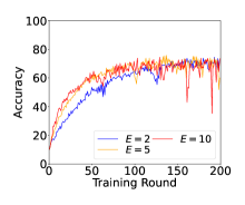
((a))

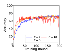
((b))

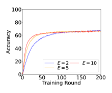
((c))

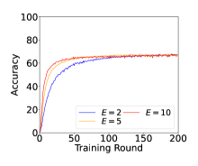
((d))

Figure 6: Impact of local iteration on SFL performance.

We further study the impact of local epoch number $E$ on the SFL performance. The results are reported in Fig. 6. We observe that SFL generally converges faster with a larger $E$, demonstrating the benefit of SFL in practical distributed systems.

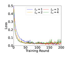
((a))

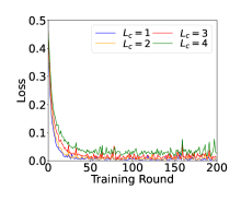
((b))

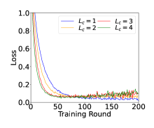
((c))

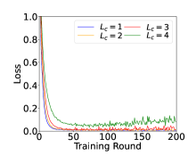
((d))

Figure 7: Impact of the choice of cut layer on SFL loss.

H.2 Results using loss metric

We further report the results using the loss metric. More specifically:

• Impact of cut layer: The results are reported in Fig. 7.

• Impact of data heterogeneity: The results are reported in Fig. 8.

• Impact of partial participation: The results are reported in Fig. 9.

In general, we see similar (but opposite) trends with the observations in the main paper. That is, a higher accuracy is associated with a smaller loss. These results are again consistent with our theories.

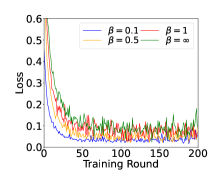
((a))

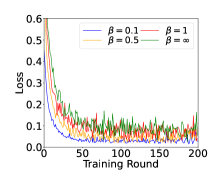
((b))

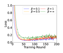
((c))

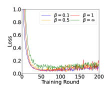
((d))

Figure 8: Impact of data heterogeneity on SFL loss.

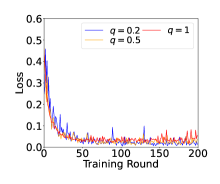
((a))

((b))

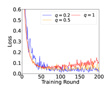
((c))

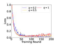
((d))

Figure 9: Impact of client participation on SFL loss.

References

- Abdelmoniem et al. (2023) Abdelmoniem, A. M., Sahu, A. N., Canini, M., and Fahmy, S. A. Refl: Resource-efficient federated learning. In Proceedings of the Eighteenth European Conference on Computer Systems, pp. 215–232, 2023.
- Gao et al. (2020) Gao, Y., Kim, M., Abuadbba, S., Kim, Y., Thapa, C., Kim, K., Camtepe, S. A., Kim, H., and Nepal, S. End-to-end evaluation of federated learning and split learning for internet of things. arXiv preprint arXiv:2003.13376, 2020.
- Han et al. (2021) Han, D.-J., Bhatti, H. I., Lee, J., and Moon, J. Accelerating federated learning with split learning on locally generated losses. In ICML workshop on federated learning for user privacy and data confidentiality, 2021.
- Han et al. (2023) Han, D.-J., Kim, D.-Y., Choi, M., Brinton, C. G., and Moon, J. Splitgp: Achieving both generalization and personalization in federated learning. Proc. of IEEE INFOCOM, 2023.
- Hsu et al. (2019) Hsu, T.-M. H., Qi, H., and Brown, M. Measuring the effects of non-identical data distribution for federated visual classification. arXiv preprint arXiv:1909.06335, 2019.
- Huang et al. (2023a) Huang, C., Ke, S., and Liu, X. Duopoly business competition in cross-silo federated learning. IEEE Transactions on Network Science and Engineering, 2023a.
- Huang et al. (2023b) Huang, C., Tian, G., and Tang, M. When minibatch sgd meets splitfed learning: Convergence analysis and performance evaluation. arXiv preprint arXiv:2308.11953, 2023b.
- Karimireddy et al. (2020) Karimireddy, S. P., Kale, S., Mohri, M., Reddi, S., Stich, S., and Suresh, A. T. Scaffold: Stochastic controlled averaging for federated learning. In International conference on machine learning, pp. 5132–5143. PMLR, 2020.
- Khaled et al. (2020) Khaled, A., Mishchenko, K., and Richtárik, P. Tighter theory for local sgd on identical and heterogeneous data. In International Conference on Artificial Intelligence and Statistics, pp. 4519–4529. PMLR, 2020.
- Koloskova et al. (2020) Koloskova, A., Loizou, N., Boreiri, S., Jaggi, M., and Stich, S. A unified theory of decentralized sgd with changing topology and local updates. In International Conference on Machine Learning, pp. 5381–5393. PMLR, 2020.
- Krizhevsky (2009) Krizhevsky, A. Learning multiple layers of features from tiny images. 2009.
- Langley (2000) Langley, P. Crafting papers on machine learning. In Langley, P. (ed.), Proceedings of the 17th International Conference on Machine Learning (ICML 2000), pp. 1207–1216, Stanford, CA, 2000. Morgan Kaufmann.
- Li et al. (2021) Li, Q., He, B., and Song, D. Model-contrastive federated learning. In Proceedings of the IEEE/CVF conference on computer vision and pattern recognition, pp. 10713–10722, 2021.
- Li et al. (2020a) Li, T., Sahu, A. K., Zaheer, M., Sanjabi, M., Talwalkar, A., and Smith, V. Federated optimization in heterogeneous networks. Proceedings of Machine learning and systems, 2:429–450, 2020a.
- Li et al. (2020b) Li, X., Huang, K., Yang, W., Wang, S., and Zhang, Z. On the convergence of fedavg on non-iid data. In Proc. of ICLR, 2020b.
- Li & Lyu (2023) Li, Y. and Lyu, X. Convergence analysis of sequential federated learning on heterogeneous data. In Thirty-seventh Conference on Neural Information Processing Systems, 2023. URL https://openreview.net/forum?id=Dxhv8Oja2V.
- McMahan et al. (2017) McMahan, B., Moore, E., Ramage, D., Hampson, S., and y Arcas, B. A. Communication-efficient learning of deep networks from decentralized data. In Artificial intelligence and statistics, pp. 1273–1282. PMLR, 2017.
- Reddi et al. (2021) Reddi, S., Charles, Z. B., Zaheer, M., Garrett, Z., Rush, K., Konečný, J., Kumar, S., and McMahan, B. (eds.). Adaptive Federated Optimization, 2021. URL https://openreview.net/forum?id=LkFG3lB13U5.
- Shen et al. (2023) Shen, J., Cheng, N., Wang, X., Lyu, F., Xu, W., Liu, Z., Aldubaikhy, K., and Shen, X. Ringsfl: An adaptive split federated learning towards taming client heterogeneity. IEEE Transactions on Mobile Computing, 2023.
- Shiranthika et al. (2023) Shiranthika, C., Kafshgari, Z. H., Saeedi, P., and Bajić, I. V. Splitfed resilience to packet loss: Where to split, that is the question. In International Conference on Medical Image Computing and Computer-Assisted Intervention, pp. 367–377. Springer, 2023.
- Stephanie et al. (2023) Stephanie, V., Khalil, I., and Atiquzzaman, M. Digital twin enabled asynchronous splitfed learning in e-healthcare systems. IEEE Journal on Selected Areas in Communications, 41(11):3650–3661, 2023. doi: 10.1109/JSAC.2023.3310103.
- Stich (2019) Stich, S. U. Unified optimal analysis of the (stochastic) gradient method. arXiv preprint arXiv:1907.04232, 2019.
- Tan et al. (2023) Tan, Y., Liu, Y., Long, G., Jiang, J., Lu, Q., and Zhang, C. Federated learning on non-iid graphs via structural knowledge sharing. In Proceedings of the AAAI conference on artificial intelligence, volume 37, pp. 9953–9961, 2023.
- Tang & Wong (2023) Tang, M. and Wong, V. W. Tackling system induced bias in federated learning: Stratification and convergence analysis. In Proc. of IEEE INFOCOM, pp. 1–10, 2023.
- Thapa et al. (2022) Thapa, C., Arachchige, P. C. M., Camtepe, S., and Sun, L. Splitfed: When federated learning meets split learning. In Proc. of AAAI, volume 36, pp. 8485–8493, 2022.
- Vepakomma et al. (2019) Vepakomma, P., Gupta, O., Swedish, T., and Raskar, R. Split learning for health: Distributed deep learning without sharing raw patient data. ICLR Workshop on AI for Social Good, 2019.
- Wang & Ji (2022) Wang, S. and Ji, M. A unified analysis of federated learning with arbitrary client participation. Advances in Neural Information Processing Systems, 35:19124–19137, 2022.
- Wang et al. (2019) Wang, S., Tuor, T., Salonidis, T., Leung, K. K., Makaya, C., He, T., and Chan, K. Adaptive federated learning in resource constrained edge computing systems. IEEE journal on selected areas in communications, 37(6):1205–1221, 2019.
- Waref & Salem (2022) Waref, D. and Salem, M. Split federated learning for emotion detection. In 2022 4th Novel Intelligent and Leading Emerging Sciences Conference (NILES), pp. 112–115. IEEE, 2022.
- Woodworth et al. (2020a) Woodworth, B., Patel, K. K., Stich, S., Dai, Z., Bullins, B., Mcmahan, B., Shamir, O., and Srebro, N. Is local sgd better than minibatch sgd? In International Conference on Machine Learning, pp. 10334–10343. PMLR, 2020a.
- Woodworth et al. (2020b) Woodworth, B. E., Patel, K. K., and Srebro, N. Minibatch vs local sgd for heterogeneous distributed learning. Advances in Neural Information Processing Systems, 33:6281–6292, 2020b.
- Wu et al. (2023) Wu, W., Li, M., Qu, K., Zhou, C., Shen, X., Zhuang, W., Li, X., and Shi, W. Split learning over wireless networks: Parallel design and resource management. IEEE Journal on Selected Areas in Communications, 41(4):1051–1066, 2023.
- Yang et al. (2021) Yang, H., Fang, M., and Liu, J. Achieving linear speedup with partial worker participation in non-iid federated learning. Proc. of ICLR, 2021.