Studying the Impact of Stochasticity on the Evaluation of Deep Neural Networks for Forest-Fire Prediction

Abstract.

This paper presents the first systematic study of the evaluation of Deep Neural Networks (DNNs) under stochastic assumptions, with a focus on wildfire prediction. We develop a framework to study the impact of stochasticity on two classes of evaluation metrics: classification-based metrics, which assess fidelity to observed ground truth (GT), and proper scoring rules, which test fidelity-to-statistic. Our findings reveal that evaluating for fidelity-to-statistic is a reliable alternative in highly stochastic scenarios. We extend our analysis to real-world wildfire data, highlighting limitations in traditional wildfire prediction evaluation methods, and suggest interpretable stochasticity-compatible alternatives.

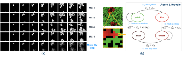
Figure 1. (a) The first four rows display four distinct realizations (MC simulations) of fire evolution from the same initial condition (fire seed location). The last row illustrates the statistic of the process, with each pixel representing the parameter of the Bernoulli distribution from which the realizations are sampled from; (b) [Left] Snapshot of forest-fire evolution in NetLogo using a 64x64 grid of agents, [Right] Flowchart depicting a single agent’s evolution rules inpired from Rothermel’s model (Rothermel, 1972).

1. Introduction

The increasing frequency and severity of wildfires underscore the need for enhanced wildfire prediction, which is critical for effective resource deployment (Westerling et al., 2006; Thompson et al., 2016). Conventional modeling tools, such as FARSITE (Finney, 1998), encounter substantial challenges due to reliance on ground-based data collection, leading to high operational costs. In response, remote sensing technology has emerged as a more efficient alternative for wildfire prediction. Utilizing satellite (Huot et al., 2022) or aircraft-based sensors (Doshi et al., 2019), remote sensing data offers expansive spatial and temporal coverage, significantly enhancing observational capabilities. This data is used to train Deep Neural Networks (DNNs) to learn the “rules” of fire evolution. Such DNNs outperform the conventional modeling tools (Radke et al., 2019) and have the potential to significantly advance wildfire management strategies.

The DNNs take observations of fire evolution over various time steps—ranging from 24 hours to a year—as input and predict fire-map evolution for future time steps, from one day to 30 days ahead, for predicting whether specific locations will burn (Huot et al., 2022; Radke et al., 2019; Yang et al., 2021). DNNs are trained using Binary Cross Entropy (BCE) loss and evaluated using conventional classification-based evaluation metrics (Ferri et al., 2009). These metrics quantify the DNN’s performance in terms of real-world decisions, and therefore, help us understand the DNN’s performance in a practical context.

Wildfires, characterized by their unpredictable evolution due to complex interactions with atmospheric conditions (Liu et al., 2021), can be modeled as a stochastic process. Here, GT is conceptualized as a distribution, represented by a random variable (RV) $X_{t}$, indexed by time $t$. In this context, DNNs in existing studies (Radke et al., 2019; Yang et al., 2021; Huot et al., 2022; Jain et al., 2020) learn from one set of random realizations (training data) and are evaluated on another (test data), each sampled from distinct stochastic processes. The prevailing training and evaluation strategy implicitly assumes that the observed GT is the sole outcome, a notion stemming from the practical constraint of observing only a single realization of the stochastic process, identified here as a deterministic bias. Implications of such stochastic interpretations on wildfire modeling is unexplored in existing research.

In this paper, we study the characteristics of evaluation metrics used for the evaluation of remote-sensing-based wildfire forecasts under stochastic assumptions. We introduce a comprehensive synthetic benchmark to systematically measure the influence of stochasticity on the applicability of the evaluation metrics employed for wildfire prediction. Our results show the reliability of evaluation metrics in terms of the variance of the stochastic process. Our findings reveal significant shortcomings such as the general inability of the studied evaluation metrics to evaluate predictions in highly stochastic scenarios. We explore alternate interpretable evaluation metrics to test the fidelity to the statistic and offer higher reliability. Key contributions of this paper include:

• We introduce a stochastic framework for high-dimensional forest fire modeling, incorporating two scales: Micro RV $M_{t,(x,y)}$ for agent-level interpretation and Macro RV $Z_{t}$ to capture the overall system’s potential states. In the context of forest fire, Micro RV represents state of the trees and Macro RV represents the state of the forest.

• Our analysis reveals a critical mismatch between DNN learning outcomes and DNN evaluation objectives. This results in increased sensitivity of the evaluation metrics to the system’s macro-variance $Var[Z_{t}]$, primarily due to the inapplicability of thresholding and false positives in scenarios where ground truth (GT) is a distribution.

• We study stochasticity-compatible metrics like Mean Squared Error (MSE) and Expected Calibration Error (ECE). MSE assesses statistical fidelity but lacks interpretability. ECE focuses exclusively on the DNN’s accuracy in predicting probabilities and adds interpretability via calibration curves.

• We extend our study to a real-world wildfire dataset (Huot et al., 2022), identifying the limitations of evaluation metrics and show interpretable alternatives.

The paper is organized as follows: §2 presents background and related work. §3 details our proposed stochastic process-based framework. In §4 we perform our experiment and examine the evaluation strategy through the lens of stochastic process. We apply our insights to a real-world wildfire dataset in §5. We discuss and conclude in §6 and §7.

Table 1. Selected works in Wildfire Prediction

Work	Window Size	DNN	Evaluation Metric
(Radke et al., 2019)	Observation: T Prediction: T+24h	CNN	F1-score, Recall, Accuracy
(Yang et al., 2021)	Observation: [T-52w, T] Prediction: T+5w	CNN+LSTM	AUC-ROC, MSE
(Huot et al., 2022)	Observation: T Prediction: T+24h	CNN	AUC-PR, Precision, Recall

Table 2. Evaluation Metrics and Descriptions

Metric	Description
Precision	Proportion of true positive predictions among all positive predictions
Recall	Proportion of true positive predictions among all actual positive instances
Accuracy	Proportion of correct predictions among all predictions
F1-score	Harmonic mean of precision and recall
AUC-PR	Area under the precision-recall curve, evaluating trade-off between precision and recall
AUC-ROC	Area under the receiver operating characteristic curve, evaluating trade-off between true positive rate and false positive rate
MSE	Mean squared error, measuring average squared difference between predicted and actual values

2. Background and Related Work

2.1. Formulation of Wildfire Modeling

Formally, wildfire evolution can be modeled on a grid of size $H\times W$, where each grid-cell $(i,j)$ at time $t$ is denoted by a binary random variable $M_{t,(i,j)}$, indicating fire presence ($1$) or absence ($0$). Let $X_{t}\in\{0,1\}^{H\times W}$ encapsulate the fire occurrence status across all cells at time $t$. Additionally, let $O_{t,(i,j)}\in\mathbb{R}^{n}$ represent an $n$-dimensional vector of observational variables (e.g., vegetation, terrain, weather conditions) for each cell at time $t$, used by DNNs like those in (Huot et al., 2022). The goal is to predict the joint conditional distribution of fire occurrences across the grid from time $t+1$ to $T$, utilizing both past fire maps and observational variables, formally given by:

(1) $$P(X_{t+1},\ldots,X_{T}|X_{1},\ldots,X_{t},O_{1},\ldots,O_{t}),$$

where $X_{1},\ldots,X_{t}$ denote the observed fire maps from the initial time to time $t$, $O_{1},\ldots,O_{t}$ are the corresponding observational variables, and $X_{t+1},\ldots,X_{T}$ are the forecasted fire maps up to time $T$.

DNN-based Modeling of wildfires The growing application of DNNs in wildfire prediction, especially with remote sensing data, is evident in key studies (Radke et al., 2019; Huot et al., 2022; Yang et al., 2021) summarized in Table 1 and reviewed comprehensively in (Jain et al., 2020). For example, FireCast (Radke et al., 2019) outperforms traditional models by 20% in predicting 24-hour wildfire perimeters using satellite imagery (Finney, 1998) (see Appendix A.1 for a taxonomy on wildfire models). These DNNs integrate various covariates like vegetation, terrain, and weather conditions; (Huot et al., 2022) use a 64 x 64-pixel grid, each containing 11 observational variables. DNNs operate in two phases for wildfire prediction: learning fire evolution rules during observation, and applying this knowledge for future predictions. Post-training, the DNNs are evaluated using evaluation metrics summarized in Table 2.

2.2. Stochasticity in wildfire evolution

Stochastic Dynamics in Wildfire Modeling and Challenges. Stochasticity plays a central role in wildfire evolution (Liu et al., 2021). It emerges from the interaction of various components—vegetation, terrain, weather conditions, and human activities (e.g., fire suppression efforts). The subtle variations in interactions can lead to significantly divergent outcomes from a given state, a phenomenon akin to the “butterfly effect” (Lorenz, 2000). These factors add noise to the rules of fire evolution that DNNs aim to learn. Despite its prevalence and significance, the influence of stochasticity has been largely overlooked in traditional deterministic approaches to wildfire modeling. Real-world data limitations, typically presenting only a single outcome from a range of possibilities, obscure the true nature of stochastic interactions. This gap limits the understanding of stochastic systems and hinders research into how stochasticity affects DNN-based modeling of real-world wildfire scenarios.

To address the limitations of real-world datasets, we create a synthetic forest-fire dataset using cellular automata-based models that simulate a wide spectrum of outcomes (see Appendix A.2 for applications of cellular automata in wildfire modeling). In our work, we utilize an agent-based model called NetLogo (Tisue and Wilensky, 2004), to implement a CA-based forest fire model. In the Agent-based formulation of Forest Fire evolution, each pixel on a spatial grid (similar to remote sensing data), is treated as an agent. Agents interact with neighbors (in the Moore neighborhood) using stochastic rules (simulated using NetLogo). The local interactions collectively drive the global fire evolution, often manifesting in complex, fractal-like patterns (see Figure 1.b). This approach allows us to study the stochastic dynamics at play in wildfire evolution, offering insights that are unconfined by the limitations of real-world data.

3. Forest Fire as a Stochastic Process

3.1. Simulating a Wildfire as a Stochastic Process

A stochastic process, represented by a sequence of random variables $Z_{1},Z_{2},\ldots,Z_{t},\ldots$, models the dynamic and unpredictable evolution of systems over time (Parzen, 1999). We model wildfire evolution as a stochastic process using $Z_{t}$. To empirically generate the stochastic process, we develop a NetLogo-based Forest-Fire model. We first establish deterministic interaction rules for neighboring agents (shown in Figure 1.b), and then add stochastic noise in the interactions (Details in Appendix B). To make the rules stochastic, we introduce $p_{\text{ignite}}$, the probability of fire after ignition conditions are met (i.e., $q>q_{\text{threshold}}$). In deterministic scenarios, $p_{\text{ignite}}$ is set to 100, ensuring ignition once the threshold is reached. A $p_{\text{ignite}}$ value of 95 indicates a 95% chance of ignition under the same conditions. The S-Level parameter is defined as $(1-p_{\text{ignite}})\times 100$, with higher S-Level values indicating more randomness in agent interactions, and an S-Level of 0 corresponding to deterministic interactions.

Empirical Stochastic Process (ESP). We represent an ESP using 1000 Monte Carlo (MC) simulations, each initiated under identical conditions (fire seed and forest configuration) and run until fuel depletion. This approach ensures variations in fire evolution stem exclusively from stochastic interactions. Figure 1.a depicts four distinct realizations of forest fire evolution (MC-1 to 4) from the same starting point. Finally, we execute a sweep of the S-Level parameter, creating an ESP for each S-Level parameter.

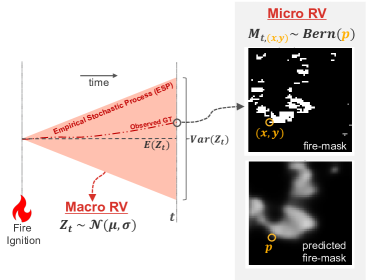
Figure 2. Illustrates the stochastic framework with Macro and Micro Random Variables (RVs) for forest fire evolution. The ESP (shaded in red) consists of 1000 Monte-Carlo (MC) Simulations, generated using a cellular-automata model.

3.2. Micro and Macro Random Variable

Addressing the challenge of modeling high-dimensional wildfire evolution, we leverage insights from statistical mechanics (Eastman, 2015) to adopt a dual-scale modeling approach. At the microscopic level, individual agent behavior is encapsulated through the Micro Random Variable (RV), $M_{t,(x,y)}$, while at the macroscopic level, the collective system behavior is represented by the Macro RV, $Z_{t}$.

Micro-Level Modeling of the Stochastic Process. At the micro level, each grid point $(x,y)$ at time $t$ is modeled by a Micro Random Variable (RV), $M_{t,(x,y)}$, following a Bernoulli distribution with expectation $E[M_{t,(x,y)}]$ equal to its probability $p$. The ensemble of Micro RVs across the grid, denoted as $\{M_{t,(x,y)}|1\leq x\leq H,1\leq y\leq W\}$, represents the grid-level micro representation of fire evolution. Parameters for each Micro RV are derived from the ESP by normalizing the burn frequency of each pixel at each timestep, across the MC simulations.

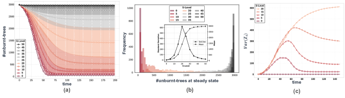
Figure 3. Characterizes the Macro RV $Z_{t}$: (a) ESP representing $Z_{t}$ across different S-Levels; (b) Histogram of $Z_{t}$ at steady state across S-Levels, with an inset showing trends in $E[Z_{t}]$ and $Var[Z_{t}]$; (c) $Var[Z_{t}]$ as a function of time fore selected test-cases.

Macro-Level Modeling of the Stochastic Process. The Macro RV, $Z_{t}$, represents the collective state of the system at time $t$. Formally, we define $Z_{t}$ as the sum of the Micro RVs across the grid:

(2) $$Z_{t}=\sum_{x=1}^{H}\sum_{y=1}^{W}M_{t,(x,y)}$$

Applying the Central Limit Theorem (due to the large number of Micro RVs $\approx 10^{3}$), $Z_{t}$ can be effectively modeled using a Normal distribution, characterized by its mean $E[Z_{t}]$ and variance $Var[Z_{t}]$. Sampling from $Z_{t}$ provides a macro-state value, representing the aggregate state of all agents. It should be noted that multiple microstates can correspond to the same macrostate value. The parameters of the Macro RV is extracted from the ESP by recording the number of unburnt trees (macrostate) at each time step and creating a distribution at each time step using the 1000 MC simulations, from which we directly compute the mean and variance to define the parameters for the macro RV.

Figure 2 summarizes the framework and shows the ESP representing the range of states fire evolution can explore as time progresses, starting from the same initial condition. The Macro RV characterizes the entire ESP using its $E[Z_{t}]$ and variance $Var[Z_{t}]$. The Micro RV focuses on the individual fire pixels and is visualized on a fire map.

3.3. Characterizing the ESP Test cases

The fifth row in Figure 1. (a) displays the Micro RV map for the ESP at S-Level 0.20, where each pixel’s value, $E[M_{t,(x,y)}]$, indicates the burn probability at that location and time, conditioned on the initial fire seed and forest configuration. This Micro RV Map, termed Statistic-GT, GT of the statistic. In practical scenarios, only a single realization (represented by an MC simulation) of the underlying stochastic process (represented by the statistic-GT) is observable.

Figure 3. (a) shows the Macro RV $Z_{t}$ over time with colors changing from red (S-Level=0) to black (S-Level=50) in increments of 5, where the central line and shaded areas denote $E[Z_{t}]$ and $Var[Z_{t}]$. Figure 3.(b) presents histograms representing $Z_{t}$ at steady state for different S-Levels, with insets showing mean and standard deviation (SD) at each level. Key observations include: At S-Level 0 (deterministic), the absence of SD implies a singular evolutionary path, an assumption implicit in current remote-sensing-based wildfire modeling (Yang et al., 2021; Huot et al., 2022; Jain et al., 2020). As S-Level increases, $Var[Z_{t}]$ peaks at 0.2, indicative of a chaotic system with multiple fire evolution pathways, aligning with real-world fire behavior (Liu et al., 2021). The SD suggests the system’s tendency towards exploring diverse macrostates, with increasing variance indicating greater unpredictability. Further increase in S-Level reduces SD and increases the mean, reflecting a rise in unburnt agents due to fire dying out in the early stages.

Figure 3.(c) displays $Var[Z_{t}]$ over time for select S-Levels used in our study. For S-Levels 5 and 10, $Var[Z_{t}]$ initially peaks, then declines, mirroring the grid’s shift towards predominantly burnt states and a consequent reduction in state space size.

3.4. Evaluation Metrics in this Study

At a high level, we classify the evaluation metrics used in our study into the following two categories:

Fidelity to Realization (F2R). Evaluation metrics like Precision, Recall, F1-score, AUC-PR are chosen for their ability to delineate type-1 and type-2 errors. These metrics are used due to (1) the binary nature of fire spread outcomes, (2) the high-risk implications of forest fire prediction, and (3) the direct link between each forecast and a decision-making action. F2R metrics are standard in DNN-based forest fire prediction.

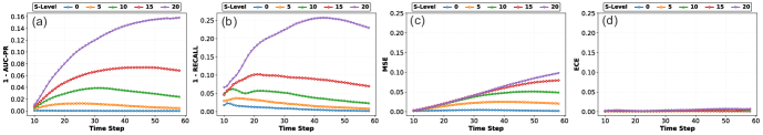
Figure 4. Performance of the DNN on the Test Split shown using (a) AUC-PR, (b) Recall, (c) MSE, and (d) ECE

Fidelity to Statistic (F2S). F2S metrics (e.g. MSE) evaluate probabilistic forecasts by comparing forecast distributions with the observed GT and are formally known as scoring rules (Gneiting and Raftery, 2007). A proper scoring rule $S$ ensures that its expected score, under the GT distribution $D_{\text{gt}}$, is minimized by an accurate forecast distribution $D_{f}$. Formally, for any forecast $D_{f}$, we have:

(3) $$\mathbb{E}_{y\sim D_{\text{gt}}}[S(y,D_{\text{gt}})]\leq\mathbb{E}_{y\sim D_{\text{gt}}}[S(y,D_{f})].$$

A scoring rule is strictly proper if this minimum is unique, offering asymptotic guarantees that the best score corresponds to the forecast matching the GT distribution. However, limitations arise with finite samples, where scoring rules may not capture basic forecasting errors (Marcotte et al., 2023). Brier Score (MSE) is a proper scoring rule (Rufibach, 2010). Scoring rules do not provide decision-based quantification of DNN’s performance (like F2R metrics), rendering them less favored in the context of wildfire prediction (Radke et al., 2019; Yang et al., 2021; Huot et al., 2022).

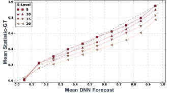
Figure 5. Shows the correlation between Statistic-GT and the DNN forecast, indicating that the DNN is learning to predict the statistic representing the stochastic process

4. Benchmark Experiment

To effectively assess DNNs in modeling forest fire evolution, understanding agent interactions is essential for accurate joint conditional distribution prediction (in Equation 1). Given the impracticality of accessing GT joint conditional distributions, evaluations typically rely on marginal distributions, treating agents independently. This approach, used by both F2R and F2S metrics, overlooks the global behavior inherent in complex systems. Thus, there’s a need to understand the impact of variability in global behavior on the DNN performance assessment in stochastic contexts.

We study the impact of macro-variance ($Var[Z_{t}]$) on the two classes of evaluation metrics: F2R and F2S. We use five different test cases with varying levels of S-Level (0,5,10,15,20) and feed it to a trained and calibrated DNN, which doesn’t have any other source of uncertainty. We examine metric responses to macro-variance using 1,000 MC simulations from the ESP. For each MC simulation, and for a given timestep, a grid of predictions at time $t$ has a corresponding $Var[Z_{t}]$, which indicates system stochasticity at that instant. As the DNN learns the statistic of the stochastic process, an ideal metric should exhibit minimal sensitivity to the system’s macro-variance.

4.1. Experiment Methodology

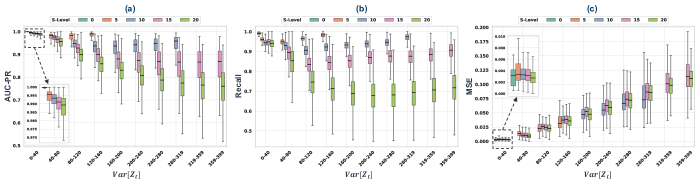
Figure 6. Impact of macro-variance $Var[Z_{t}]$ on the performance of the DNN using (a) AUC-PR (b) Recall, and (c) MSE

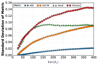
Figure 7. Shows the SD of the evaluation metrics vs. $Var[Z_{t}]$; higher values indicates higher sensitivity to $Var[Z_{t}]$.

Generating Calibrated DNNs. We created convLSTM-CA, a modified convLSTM architecture that retains spatial information (see §C.1). Our dataset contains 1,000 forest fire simulations with S-Levels from 0 (deterministic) to 20 (highly stochastic), in increments of 5. Each simulation, unique in fire seed and forest layout, represents a single realization of the stochastic process, mirroring real-world diversity. The DNNs train on one set of these realizations and are tested on another, providing a controlled environment that replicates practical training and evaluation scenarios. The training dataset, comprising 700 simulations, was segmented into 60-frame intervals. The DNN initially observes the first 10 frames in RGB, then predicts the next 50 frames using binary segmentation (1 for burnt, 0 for unburnt areas). We utilize BCE loss for training.

Calibration with the statistic-GT. In Figure 5, we plot the mean statistic-GT against the corresponding mean DNN Forecast. The correlation between them indicates that the DNN is learning to predict the statistic-GT. This ability to learn and predict stochastic fire evolution is linked to the use of BCE loss (a proper scoring rule), which ensures calibrated forecasts by learning the true probability distribution of the process (Gneiting and Raftery, 2007) (details in §C.3).

4.2. DNN Prediction in short versus long horizon

Figure 4.a-c shows the performance of the DNN for five test cases using AUC-PR, Recall, and MSE, using the test split of 300 simulations. For a given time step, the evaluation score is calculated by combining the predictions and GT across the 300 simulations. We observe a trend of evaluation metrics falling as S-Level increases and a decrease in value for long-horizon predictions. This evaluation strategy assumes the test split’s GT as the only outcome (a deterministic bias), and contradicts our conclusion from Figure 5. The observed trend in Figure 4.a-c does not indicate the DNN’s inability to learn the stochastic process, and we revisit this in §4.3.

4.3. Impact of Macro-Variance on metrics

F2R metrics vs. macro-variance. Figure 6.a and b shows the relationship between DNN performance (AUC-PR, Recall) and system macro-variance ($Var[Z_{t}]$), revealing an inverse monotonic relationship. Notably, the confidence width of these metrics widens with increased $Var[Z_{t}]$. Figure 7 further underscores this trend, showing the Standard Deviation (SD) of metrics against $Var[Z_{t}]$. The steep rise in SD for F2R metrics (Precision, Recall, AUC-PR) highlights their heightened sensitivity to macro-variance.

Discussion on F2R Metrics in Stochastic Contexts. Precision and Recall exhibit high variance in stochastic settings due to their reliance on thresholding. Applying a threshold to a DNN’s forecast map produces a specific predictive outcome that may not match the actual GT, a discrepancy arising from the incompatibility of “thresholding” with stochastic processes. This critique is different from the usual critique of arbitrary threshold selection, such as a 0.5 cutoff (Fourure et al., 2021). Metrics like AUC-PR, though less sensitive than threshold-based metrics, still face challenges due to their incorporation of False Positives (FP) via Precision. In stochastic contexts, the traditional concept of FP loses relevance since any non-zero forecast by the DNN renders both outcomes (1 and 0) plausible.

F2S metrics vs. macro-variance. Compared to F2R, MSE shows less sensitivity to the macro-variance of the system, as seen in Figure 6.c and Figure 7. This is attributed to MSE’s mathematical robustness as a strictly proper scoring rule, ensuring it attains minimum value only when the DNN accurately learns the underlying stochastic process’s true distribution (Gneiting and Raftery, 2007). We can also observe a monotonic trend between MSE and macro-variance in Figure 6.c. This can be explained by the Brier Score decomposition of the MSE: (Rufibach, 2010).

(4) $$\text{MSE}=\text{E}[(\text{E}[O|F]-F)^{2}]+\text{E}[\text{Var}(O|F)]$$

It decomposes into two components: Reliability (or Calibration Error) and inherent outcome variability. The Reliability component, $\text{E}[(\text{E}[O|F]-F)^{2}]$, measures probabilistic accuracy. The second component, $\text{E}[\text{Var}(O|F)]$, quantifies the portion of total outcome variance unexplained by the forecasts, representing inherent uncertainty, which shows up in Figure 6.c.

4.4. Calibration Error

Subtracting inherent outcome variability from MSE (refer to Equation 4) isolates calibration error, which specifically assesses forecast accuracy. Calibration error benefits from asymptotic guarantees and can be visualized via calibration curves, adding interpretability.

Expected Calibration Error (ECE) (Naeini et al., 2015), a prevalent metric for measuring calibration error, is defined for grid-based predictions as:

(5) $$\text{ECE}=\sum_{k=1}^{m}\frac{|I_{k}|}{N}\left|\text{acc}(I_{k})-\text{conf}(I_{k})\right|$$

where $m$ is the number of intervals, $I_{k}$ is the $k$-th interval of predicted probabilities, $|I_{k}|$ denotes the number of grid location predictions in $I_{k}$, and $N$ represents the total number of grid location predictions across all samples. The term $\text{acc}(I_{k})$ signifies the accuracy within interval $I_{k}$, calculated as the proportion of correct predictions at the grid locations, while $\text{conf}(I_{k})$ denotes the average predicted probability within $I_{k}$.

Added interpretability to ECE using calibration curves. The calibration curve is an interpretable tool to intuitively understand the deviation between the model and the estimated probability in ECE. Given a set of frames (in a test dataset) $\{G_{n}\}_{n=1}^{N}$, where each $G_{n}$ represents a grid of dimension $H\times W$, let $p_{n,i,j}=F(G_{n})_{i,j}\in[0,1]$ represent the forecasted probability by the classifier for each location $(i,j)$ within the grid $G_{n}$. These probabilities $p_{n,i,j}$ are grouped into intervals $I_{k}$ for $k=1,2,\ldots,m$, partitioning the range [0, 1] (e.g., [0, 0.1], (0.1, 0.2], etc.). A calibration curve is then constructed by plotting the predicted average probability $\overline{p_{k}}=\frac{1}{N_{k}}\sum_{n,i,j:p_{n,i,j}\in I_{k}}p_{n,i,j}$ for each interval $I_{k}$ against the observed empirical average $\overline{y_{k}}=\frac{1}{N_{k}}\sum_{n,i,j:p_{n,i,j}\in I_{k}}y_{n,i,j}$, where $y_{n,i,j}$ is the GT for the location $(i,j)$ in grid $G_{n}$, and $N_{k}=|\{(n,i,j):p_{n,i,j}\in I_{k}\}|$ represents the total number of predictions in interval $I_{k}$. Perfect calibration is indicated by the calibration curve forming a straight line, with an interpretable intuition backing the curve, out of all the predictions the DNN made with p x, x% actually burnt, tying down the metric to real-world actions.

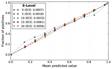
Figure 8. Calibration curve using Test split (ECE in legend)

ECE Results on the Test split. In Figure 8.a, calibration curves for the entire test split (outlined in Section 4.1) are shown with their Expected Calibration Error (ECE) in the legend. The time-stratified ECE values are shown in Figure 4.d indicating that long-duration predictions measured by ECE are doing good, indicating that the DNN is statistically sound. The calibration curve indicates that the DNN is predicting accurate probabilities (see §D for use-case of ECE).

Next, we extend our observations to a real-world forest fire dataset. In the real-world dataset, $Var[Z_{t}]$ is not available, as we observe one realization of $Z_{t}$. However, we can still see the effect of stochasticity in the qualitatives, where fire pixels randomly jump around (highlighted with low Dice Coefficient scores calculated between successive fire masks) shown in Figure 9.

5. Application to Real World Wildfire

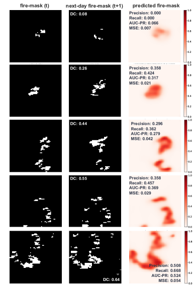
Figure 9. The DNN takes as input fire mask (left column) alongside 11 observational variables to forecast the next-day fire mask (right column), compared against the observed ground truth (GT) in the middle column. Evaluation through F2R metrics indicates suboptimal performance, whereas the MSE score, despite being low, does not adequately reflect the DNN’s practical efficacy.

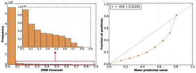
Figure 10. [Left] displays the distribution histogram of forecasts generated by the DNN; [Right] shows a Calibration Curve that illustrates forecast accuracy in an interpretable manner. This curve suggests (1) the DNN’s tendency towards overconfidence in mid-range forecasts, and (2) the accuracy of its probabilistic predictions is better for forecasts at the lower and upper ends of the probability spectrum.

5.1. Methodology

Dataset. The Next Day Wildfire Spread dataset consolidates historical wildfire incidents with 11 observational variables onto two-dimensional regions with a 1 km resolution (Huot et al., 2022). These variables, which include elevation, wind direction and speed, minimum and maximum temperature, humidity, precipitation, drought index, vegetation, population density, and the Energy Release Component (ERC). The dataset documents 18,545 wildfire events and provides sequential snapshots of fire spread, captured at time $t$ and $t+1$ day.

DNN Model. Following Huot et al.’s methodology, we replicated their convolutional autoencoder model (Huot et al., 2022). The DNN takes as input a spatial map of 11 observational variables and fire spread at time $t$, and predicts the binary segmentation map representing fire spread at time $t+1$. Figure 9 shows the fire mask at time $t$ (left column), the next-day fire mask at time $t+1$ (the observed GT), and the raw forecast from the DNN.

Experiment. Since real-world wildfire is stochastic, our goal is to understand its impact on the DNN’s evaluation. The low overall scores reported by the authors indicate that the DNN is performing badly, but the qualitatives discussed by the authors indicate that the DNN is performing good. We hypothesize that such a disconnect is arising due to the highly stochastic nature of the wildfire, which messes up the F2R metrics used by the authors (as observed in Section 4). Our goal is to re-evaluate the DNN’s predictions under our new learnings.

5.2. Results

Huot et al. reported the overall scores of Precision, Recall, and AUC-PR in their works. We use the Dice Coefficient (DC) calculated between the fire mask and the next-day fire mask to measure how much the fire mask has evolved. We then stratify the scores using the DC values and report our results in Table 3. Higher DC values indicate evolutionary fire progression, while lower DC values point to abrupt changes in fire fronts. For example, in Figure 9, for the first sample a DC of 0.08 indicates that the fire front has completely moved from its original location, while the last sample has a DC of 0.64 suggesting a slower progression from time $t$ to $t+1$.

In Table 3, as we move from top to bottom, DC decreases indicating that the level of overlap decreases. We can observe that, in general, the evaluation metrics decrease in value as DC decreases. The lowest scores for Precision, Recall, and AUC-PR are reported for DC 0-0.1, however, for MSE, the score for DC 0-0.1 is lower than the other bins, indicating that probabilistically the DNN is making fewer errors. However, the raw values of the MSE do not provide information about the practical utility of the DNN.

Calibration Curve for the Next-Day-Wildfire dataset. Figure 10 shows the histogram of the DNN’s predictions over the entire test split on the left and the calibration curve on the right. We can observe from the calibration, that the DNN is making overconfident predictions for the middle probability region, but the overall performance of the DNN is not as bad as F2R-based evaluation metrics portray.

Table 3. Evaluation metrics for the Next-Day-Wildfire-Spread dataset (Huot et al., 2022), stratified by the DC value ($\uparrow:$ Slower fire progression).

DC	Support	Precision$\uparrow$ (95% CI)	Recall$\uparrow$ (95% CI)	AUC-PR$\uparrow$ (95% CI)	MSE$\downarrow$ (95% CI)
0.9-1.0	1	0.000 (NA, NA)	0.000 (NA, NA)	1.000 (NA, NA)	0.000 (NA, NA)
0.8-0.9	4	0.000 (0.000, 0.000)	0.000 (0.000, 0.000)	0.459 (0.142, 0.776)	0.001 (0.001, 0.001)
0.7-0.8	3	0.518 (0.000, 0.913)	0.463 (0.000, 0.889)	0.712 (0.591, 0.812)	0.003 (0.001, 0.005)
0.6-0.7	75	0.392 (0.332, 0.457)	0.509 (0.431, 0.584)	0.599 (0.544, 0.649)	0.013 (0.010, 0.016)
0.5-0.6	116	0.420 (0.381, 0.458)	0.524 (0.475, 0.571)	0.547 (0.518, 0.574)	0.019 (0.016, 0.022)
0.4-0.5	145	0.391 (0.357, 0.429)	0.466 (0.428, 0.505)	0.423 (0.394, 0.452)	0.016 (0.014, 0.019)
0.3-0.4	142	0.290 (0.257, 0.322)	0.347 (0.308, 0.391)	0.378 (0.350, 0.412)	0.019 (0.016, 0.021)
0.2-0.3	217	0.202 (0.178, 0.226)	0.251 (0.216, 0.286)	0.306 (0.280, 0.333)	0.017 (0.015, 0.020)
0.1-0.2	150	0.217 (0.176, 0.263)	0.159 (0.127, 0.193)	0.251 (0.220, 0.283)	0.017 (0.015, 0.020)
0.0-0.1	836	0.021 (0.015, 0.028)	0.020 (0.014, 0.027)	0.038 (0.032, 0.045)	0.007 (0.006, 0.008)
Overall	1689	0.298	0.404	0.248	0.014

6. Discussion

Related Works in Stochastic Video Prediction. Stochasticity has been studied in video prediction to address predictions where deterministic models fall short, as surveyed in (Oprea et al., 2022). While deterministic prediction is effective in predictable contexts (e.g., car movement on a straight trajectory), it struggles with sporadic unpredictable events (e.g., car turning). In such cases, deterministic DNNs predict an average of all possible outcomes, leading to blurry predictions (Mathieu et al., 2016). Therefore, the focus is on developing stochastic DNNs that offer a range of potential outcomes with high contrast rather than a single blurry prediction. This involves learning a latent variable, and besampling from it to generate diverse realizations. For evaluation, the authors report the best score across different generated samples, testing for fidelity to individual realization (Henaff et al., 2017). Unlike the sporadic nature of stochasticity in video prediction, wildfires exhibit stochasticity consistently (Gallager, 2013). This challenges the application of stochastic DNNs, which face issues of uncontrollable and variable quality predictions due to their focus on making high-contrast predictions (Jin et al., 2020), thereby making it a less suitable strategy for high-risk wildfire prediction. Our study diverges from traditional stochastic video prediction, emphasizing fidelity to statistical outcomes as a more suitable strategy for high-risk wildfire prediction, contingent on proper interpretation and evaluation. By providing stochastic interpretation and stochasticity-compatible evaluation methods, we aim to enhance the reliability of DNNs in stochastic wildfire prediction.

Macro-variance as an Aleatoric (Irreducible) Uncertainty. The use of calibration curves is popular in deep learning for measuring the quality of the uncertainty estimates. Predictive uncertainty in traditional deterministic pipelines like image classification tasks, manifests in two forms: data uncertainty and model uncertainty (Abdar et al., 2021). While data uncertainty is due to measurement errors causing class overlaps, model uncertainty emerges from the model’s unfamiliarity with specific data points which can be attributed to out-of-distribution data or limited model capacity (Malinin and Gales, 2018). But both these uncertainties arise from limitations of the DNN pipeline and do not represent the fundamental property of the system. What we observe in this work is the aleatoric uncertainty which shows up due to the macro variance of the system under study.

Generalization to binary-classification problems. The implications of our study extend beyond wildfire prediction, offering insights into the evaluation of Deep Neural Networks (DNNs) across a spectrum of binary classification tasks within natural and social systems. Systems such as the spread of epidemics (Ghosh and Bhattacharya, 2020; White et al., 2007) and the propagation of rumors in social networks (Wang et al., 2014; Kawachi et al., 2008), characterized by dynamic elements and discrete state transitions, similarly exhibit complex global behaviors arising from simple local interactions. Our findings suggest that traditional evaluation metrics, which focus on fidelity to observed GT, may not adequately capture the DNN’s ability to learn the stochastic interactions present in the system. A low value of these metrics, while not desirable, does not necessarily indicate the DNN’s inability to learn the stochastic system. Instead, stochasticity-compatible metrics like Mean Squared Error (MSE) and Calibration Curves, which assess fidelity to statistical patterns, could offer more reliable and interpretable assessments. This approach, validated in the context of wildfire prediction, has the potential to enhance model evaluation in other domains where outcomes are inherently stochastic, ensuring that DNNs are comprehensively assessed for their predictive performance.

7. Conclusion

In this paper, we have introduced a stochastic framework for modeling wildfire evolution, integrating both micro and macro-scale perspectives to model the inherent unpredictability of fire spread. Through systematic analysis, we’ve characterized the behavior of two classes of evaluation metrics (F2R,F2S), when applied to wildfire prediction under stochastic conditions. Our findings suggest that commonly used metrics like Precision, Recall, and AUC-PR exhibit increased sensitivity to the macro-variance of the system, and do not evaluate a DNN’s capability to predict the statistic We studied alternate stochasticity-compatible metrics, such as MSE and ECE, which offer more reliable assessments by focusing on statistical fidelity and enhancing interpretability through calibration curves. Extending our framework to a real-world wildfire dataset further validates the necessity of reevaluating current evaluation practices to ensure they account for the stochastic nature of wildfires. Our work not only sheds light on the complexities of evaluating DNNs in stochastic systems but also paves the way for developing more robust and interpretable evaluation strategies for such systems.

8. Acknowledgement

The authors thank Hemant Kumawat and Minah Lee for the insightful discussions. This work was supported in part by the Office of Naval Research under Grant N00014-20-1-2432. The views and conclusions contained in this document are those of the authors and should not be interpreted as representing the official policies, either expressed or implied, of the Office of Naval Research or the U.S. Government.

Appendix A Literature Survey

A.1. Models for forest fire modeling

Currently, forest fire spread models are categorized into three classes: empirical, semi-empirical, and physical. Empirical models, e.g., DNN modeling using remote sensing data (Jain et al., 2020), analyze fire data statistically without exploring combustion mechanisms. Semi-empirical models, often the preferred choice, like (Finney, 1998; Rothermel, 1972) integrate physical laws, such as heat transfer, but necessitate resource-intensive ground surveys for calculating model parameters (Finney, 1998). Physical models, involving complex equations for heat dynamics (Séro-Guillaume and Margerit, 2002), are too complex for broad application. All these classes of models are deterministic and do not capture the stochastic nature of real-world fire dynamics.

A.2. Cellular Automata in wildfire applications

Cellular Automata (CA) models, with each pixel acting as an individual agent, offer a natural way to simulate stochastic interactions. These models, defined by discrete space and time, and marked by local spatial interactions, align well with the geographical nature of forest fires (Gouveia Freire and Castro DaCamara, 2019). In CA-based forest fire models, each cell on fire is an agent capable of spreading the fire based on neighborhood interaction rules, leading to emergent behaviors that mirror real-life fire propagation patterns (Zinck and Grimm, 2008; Bak et al., 1987). CA models have been employed for various purposes in wildfire modeling, such as learning fire spread rules (Zan et al., 2022), learning parameters influencing agent interactions (Li et al., 2022), and investigating chaos in fire evolution using Mean Field techniques (Malarz et al., 2002).

Appendix B NetLogo Model

The simulation starts on a $64\times 64$ grid, with each pixel initialized as a ‘tree’ or ‘no-tree’. Agents have heat values $q_{(i,j)}$ crucial for the heat transfer in forest fire evolution. Fire seeds, placed at randomized (or fixed) locations, provide initial heat to agents. The initial condition is set as $q_{(i,j)}=I_{\text{seed}}\times q_{\text{threshold}}$ for seed locations $(i,j)$, and $q_{(i,j)}=0$ otherwise, where $q_{\text{threshold}}$ is the ignition threshold and $I_{\text{seed}}$ amplifies seed heat values. A ‘tree’ agent accumulates heat from activated neighbors in its Moore neighborhood, in line with heat transfer mechanisms described by (Rothermel, 1972), following the equation:

(6) $$q_{(i,j)}(t+\Delta t)=q_{(i,j)}(t)+\sum_{(k,l)\in N_{R}}\mathbf{1}_{(k,l)}(t)q_{(k,l)}(t)$$

The indicator function $\mathbf{1}_{(k,l)}(t)$ ensures only ‘fire’ state agents contribute to heat transfer. An agent’s heat value $q_{(i,j)}$ exceeding $q_{\text{threshold}}$ triggers a state change from ‘patch’ to ‘fire’, and then to ‘ember’ in the next time step. ‘Ember’ agents radiate heat at a rate of $q_{\text{die}}$ to adjacent non-fire patches, gradually losing heat until radiation ceases. This process ends when ‘ember’ agents darken, indicating $q_{(i,j)}$ falling below a certain threshold, thus terminating heat radiation and transitioning to the ‘dead’ state.

Appendix C Characterizing the DNN

C.1. Design Rationale behind convLSTM-CA

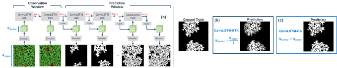
Figure 11. (a) Auto-regressive training of the DNN, (b) Softmax probability map from a convLSTM with a bottleneck, and (c) Softmax probability map from convLSTM-CA with no bottleneck.

The ConvLSTM architecture is chosen for its ability to efficiently model spatiotemporal systems, aligning well with the characteristics of the Forest-Fire system. Our modified version (see Figure 11.(a)), convLSTM-CA, places a ConvLSTM cell with a $3\times 3$ kernel between an Encoder (with a $3\times 3$ kernel) and a Decoder (with a $1\times 1$ kernel). The Encoder takes an RGB image and transforms it into a latent tensor during a 10-timestep observation window. This tensor is then processed by the ConvLSTM cell, maintaining its spatial dimensions, before the Decoder produces a burnt map grid of softmax probabilities.

This design choice of preserving spatial dimensions is crucial. Reducing the spatial dimensions of the latent tensor is a popular design choice in video prediction models such as recurrent neural network-based (Wang et al., 2017, 2018) and simple CNN-based models (Gao et al., 2022). This reduction is often employed to decrease computational complexity and to capture essential spatial features while discarding less informative details. However, we observe that adding a bottleneck causes individual pixels (agents) to lose their identity. Maintaining these dimensions helps preserve each agent’s identity, a critical factor for developing a DNN that minimizes mis-calibrated forecasts arising from limited model capacity. For instance, as seen in Figure 11. (b), using a compressed latent dimension results in a forecast cloud around predictions for deterministic fire evolution scenarios, which does not accurately reflect the system’s true evolution. In contrast, as shown in Figure 11.(c) an uncompressed latent space yields predictions without a forecast cloud, aligning closely with the deterministic system’s true evolutionary rules.

C.2. Qualitative Visualizations of DNN Forecasts

Figure 11 shows different instances of DNN Predictions.

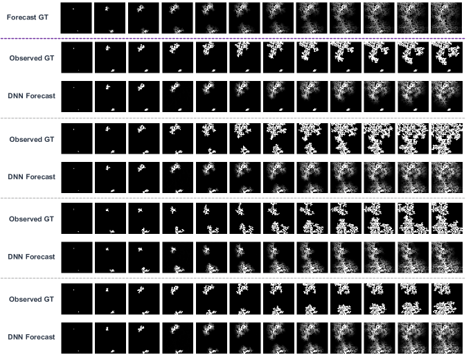
Figure 12. Qualitative Visualizations of the DNN’s forecasts for four different MC simulations. Frames are shown every five time steps. The DNN observes the first 10 time steps (first 2 frames) and predicts the next 50 time steps (last 10 frames). We can observe the difference between the DNN’s forecasts and the statistic GT, which arises because of the determinism that is injected into the DNN’s predictions due to its observation of the first 10 frames of the fire evolution.

C.3. Visualizing DNN’s predictions using ESP

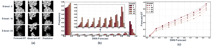
Figure 13. (a) Qualitative visualizations of forest-fire snapshots for different S-Level (one per row) showing statistic-GT, observed GT, and the corresponding DNN Prediction (raw forecast values); (b) Histogram shows the frequency of DNN’s forecast values for different S-Level values. We can observe that the DNN’s prediction becomes less confident with an increase in S-Level; (c) Line plot shows that the predicted forecast values follow the calibration trajectory, indicating that the DNN is predicting forecasts which are proportional to the ground truth forecast values.

Figure 13.a shows the DNN’s raw outputs, Statistic-GT, and Observed-GT (MC sample) for various S-levels, where higher S-Levels correlate with greater ‘cloudiness’ in DNN output. Figure 13.b illustrates histograms of DNN predictions across 1000 simulations for each S-Level. In deterministic settings, predictions are mainly binary (1 or 0), but at S-Level 20, predictions span the 0-1 range, indicating increased predictive uncertainty in highly stochastic scenarios. This ability to learn and predict stochastic fire evolution is linked to the use of BCE loss, which ensures calibrated forecasts by learning the true probability distribution of the process (Gneiting and Raftery, 2007).

Figure 13.c compares the DNN’s raw predictions with the Statistic-GT values. The y-axis plots the mean Statistic-GT, and the x-axis, the mean DNN predictions. A monotonic trend suggests the DNN learns to predict the statistic $E[M_{t,(x,y)}]$ from observing initial fire evolution in a single realization. Higher S-Levels introduce some mis-calibration, a result of determinism from observing the initial 10 frames (see Appendix C.2).

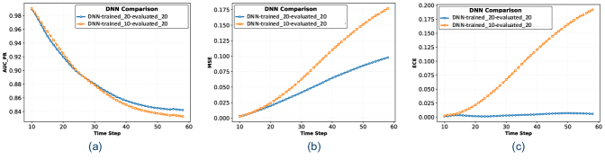
Figure 14. Use case of ECE: Evaluate whether the DNN has learnt a stochastic process using (a) AUC-PR, (b) MSE, and (c), ECE

Appendix D Evaluating the statistic

In this experiment we evaluate what happens when the DNN learns from one s-level and is evaluated on the other. In this specific example, one DNN is trained on S-Level 20 and the other is trained on S-Level 10. They are both evaluated on S-Level 20. Figure 14 shows the performance of the two DNNs reported by AUC-PR, MSE, and ECE. AUC-PR doesn’t show any difference between the two DNNs, as it’s not evaluating the statistic. MSE and BCE show visible difference. ECE shows the steepest difference because the DNN learnt a different noisy interaction rule, affecting the probabilistic accuracy. The system variance common in both test cases, reduces the gap in MSE.

References

- (1)
- Abdar et al. (2021) Moloud Abdar, Farhad Pourpanah, Sadiq Hussain, Dana Rezazadegan, Li Liu, Mohammad Ghavamzadeh, Paul Fieguth, Xiaochun Cao, Abbas Khosravi, U. Rajendra Acharya, Vladimir Makarenkov, and Saeid Nahavandi. 2021. A review of uncertainty quantification in deep learning: Techniques, applications and challenges. Information Fusion 76 (Dec. 2021), 243–297. https://doi.org/10.1016/j.inffus.2021.05.008
- Bak et al. (1987) Per Bak, Chao Tang, and Kurt Wiesenfeld. 1987. Self-organized criticality: An explanation of the 1/f noise. Phys. Rev. Lett. 59 (Jul 1987), 381–384. Issue 4. https://doi.org/10.1103/PhysRevLett.59.381
- Doshi et al. (2019) Jigar Doshi, Dominic Garcia, Cliff Massey, Pablo Llueca, Nicolas Borensztein, Michael Baird, Matthew Cook, and Devaki Raj. 2019. FireNet: Real-time Segmentation of Fire Perimeter from Aerial Video. arXiv:1910.06407 [cs.CV]
- Eastman (2015) Peter Eastman. 2015. Introduction to Statistical Mechanics. https://web.stanford.edu/~peastman/statmech/. https://web.stanford.edu/~peastman/statmech/ Accessed: [insert date of access].
- Ferri et al. (2009) C. Ferri, J. Hernández-Orallo, and R. Modroiu. 2009. An experimental comparison of performance measures for classification. Pattern Recognition Letters 30, 1 (Jan. 2009), 27–38. https://doi.org/10.1016/j.patrec.2008.08.010
- Finney (1998) Mark A. Finney. 1998. FARSITE: Fire Area Simulator-model development and evaluation. Technical Report. https://doi.org/10.2737/rmrs-rp-4
- Fourure et al. (2021) Damien Fourure, Muhammad Usama Javaid, Nicolas Posocco, and Simon Tihon. 2021. Anomaly Detection: How to Artificially Increase Your F1-Score with a Biased Evaluation Protocol. In Machine Learning and Knowledge Discovery in Databases. Applied Data Science Track (Lecture Notes in Computer Science), Yuxiao Dong, Nicolas Kourtellis, Barbara Hammer, and Jose A. Lozano (Eds.). Springer International Publishing, Cham, 3–18. https://doi.org/10.1007/978-3-030-86514-6_1
- Gallager (2013) Robert G. Gallager. 2013. Stochastic Processes: Theory for Applications. Cambridge University Press. https://doi.org/10.1017/CBO9781139626514
- Gao et al. (2022) Zhangyang Gao, Cheng Tan, Lirong Wu, and Stan Z Li. 2022. Simvp: Simpler yet better video prediction. In Proceedings of the IEEE/CVF Conference on Computer Vision and Pattern Recognition. 3170–3180.
- Ghosh and Bhattacharya (2020) Sayantari Ghosh and Saumik Bhattacharya. 2020. A data-driven understanding of COVID-19 dynamics using sequential genetic algorithm based probabilistic cellular automata. Applied Soft Computing 96 (2020), 106692.
- Gneiting and Raftery (2007) Tilmann Gneiting and Adrian E Raftery. 2007. Strictly proper scoring rules, prediction, and estimation. Journal of the American statistical Association 102, 477 (2007), 359–378.
- Gouveia Freire and Castro DaCamara (2019) Joana Gouveia Freire and Carlos Castro DaCamara. 2019. Using cellular automata to simulate wildfire propagation and to assist in fire management. Natural Hazards and Earth System Sciences 19, 1 (Jan. 2019), 169–179. https://doi.org/10.5194/nhess-19-169-2019
- Henaff et al. (2017) Mikael Henaff, Junbo Zhao, and Yann LeCun. 2017. Prediction Under Uncertainty with Error-Encoding Networks. arXiv:1711.04994 [cs.AI]
- Huot et al. (2022) Fantine Huot, R. Lily Hu, Nita Goyal, Tharun Sankar, Matthias Ihme, and Yi-Fan Chen. 2022. Next Day Wildfire Spread: A Machine Learning Dataset to Predict Wildfire Spreading From Remote-Sensing Data. IEEE Transactions on Geoscience and Remote Sensing 60 (2022), 1–13. https://doi.org/10.1109/TGRS.2022.3192974
- Jain et al. (2020) Piyush Jain, Sean C.P. Coogan, Sriram Ganapathi Subramanian, Mark Crowley, Steve Taylor, and Mike D. Flannigan. 2020. A review of machine learning applications in wildfire science and management. Environmental Reviews 28, 4 (2020), 478–505. https://doi.org/10.1139/er-2020-0019 arXiv:https://doi.org/10.1139/er-2020-0019
- Jin et al. (2020) Beibei Jin, Yu Hu, Qiankun Tang, Jingyu Niu, Zhiping Shi, Yinhe Han, and Xiaowei Li. 2020. Exploring Spatial-Temporal Multi-Frequency Analysis for High-Fidelity and Temporal-Consistency Video Prediction. In Proceedings of the IEEE/CVF Conference on Computer Vision and Pattern Recognition (CVPR).
- Kawachi et al. (2008) Kazuki Kawachi, Motohide Seki, Hiraku Yoshida, Yohei Otake, Katsuhide Warashina, and Hiroshi Ueda. 2008. A rumor transmission model with various contact interactions. Journal of theoretical biology 253, 1 (2008), 55–60.
- Li et al. (2022) Xingdong Li, Mingxian Zhang, Shiyu Zhang, Jiuqing Liu, Shufa Sun, Tongxin Hu, and Long Sun. 2022. Simulating Forest Fire Spread with Cellular Automation Driven by a LSTM Based Speed Model. Fire 5, 1 (Jan. 2022), 13. https://doi.org/10.3390/fire5010013
- Liu et al. (2021) Naian Liu, Jiao Lei, Gao Wei, Haixiang Chen, and Xiaodong Xie. 2021. Combustion dynamics of large-scale wildfires. Proceedings of the Combustion Institute 38 (01 2021). https://doi.org/10.1016/j.proci.2020.11.006
- Lorenz (2000) Edward Lorenz. 2000. The butterfly effect. World Scientific Series on Nonlinear Science Series A 39 (2000), 91–94.
- Malarz et al. (2002) K. Malarz, S. Kaczanowska, and K. Kulakwoski. 2002. Are Forest Fires Predictable? International Journal of Modern Physics C 13, 08 (2002), 1017–1031. https://doi.org/10.1142/S0129183102003760 arXiv:https://doi.org/10.1142/S0129183102003760
- Malinin and Gales (2018) Andrey Malinin and Mark Gales. 2018. Predictive Uncertainty Estimation via Prior Networks. arXiv:1802.10501 [stat.ML]
- Marcotte et al. (2023) Étienne Marcotte, Valentina Zantedeschi, Alexandre Drouin, and Nicolas Chapados. 2023. Regions of reliability in the evaluation of multivariate probabilistic forecasts. In Proceedings of the 40th International Conference on Machine Learning (Honolulu, Hawaii, USA) (ICML’23). JMLR.org, Article 999, 47 pages.
- Mathieu et al. (2016) Michael Mathieu, Camille Couprie, and Yann LeCun. 2016. Deep multi-scale video prediction beyond mean square error. arXiv:1511.05440 [cs.LG]
- Naeini et al. (2015) Mahdi Pakdaman Naeini, Gregory Cooper, and Milos Hauskrecht. 2015. Obtaining well calibrated probabilities using bayesian binning. In Proceedings of the AAAI conference on artificial intelligence, Vol. 29.
- Oprea et al. (2022) Sergiu Oprea, Pablo Martinez-Gonzalez, Alberto Garcia-Garcia, John Alejandro Castro-Vargas, Sergio Orts-Escolano, Jose Garcia-Rodriguez, and Antonis Argyros. 2022. A Review on Deep Learning Techniques for Video Prediction. IEEE Transactions on Pattern Analysis and Machine Intelligence 44, 6 (2022), 2806–2826. https://doi.org/10.1109/TPAMI.2020.3045007
- Parzen (1999) Emanuel Parzen. 1999. Stochastic Processes.
- Radke et al. (2019) David Radke, Anna Hessler, and Dan Ellsworth. 2019. Firecast: Leveraging Deep Learning to Predict Wildfire Spread. In Proceedings of the 28th International Joint Conference on Artificial Intelligence (Macao, China) (IJCAI’19). AAAI Press, 4575–4581.
- Rothermel (1972) Richard C Rothermel. 1972. A mathematical model for predicting fire spread in wildland fuels. Vol. 115. Intermountain Forest & Range Experiment Station, Forest Service, US ….
- Rufibach (2010) Kaspar Rufibach. 2010. Use of Brier score to assess binary predictions. Journal of clinical epidemiology 63, 8 (2010), 938–939.
- Sofaer et al. (2019) Helen R. Sofaer, Jennifer A. Hoeting, and Catherine S. Jarnevich. 2019. The area under the precision-recall curve as a performance metric for rare binary events. Methods in Ecology and Evolution 10, 4 (2019), 565–577. https://doi.org/10.1111/2041-210X.13140 arXiv:https://besjournals.onlinelibrary.wiley.com/doi/pdf/10.1111/2041-210X.13140
- Séro-Guillaume and Margerit (2002) O. Séro-Guillaume and J. Margerit. 2002. Modelling forest fires. Part I: A complete set of equations derived by extended irreversible thermodynamics. International Journal of Heat and Mass Transfer 45 (04 2002), 1705–1722. https://doi.org/10.1016/S0017-9310(01)00248-4
- Thompson et al. (2016) Matthew Thompson, Phil Bowden, April Brough, Joe Scott, Julie Gilbertson-Day, Alan Taylor, Jennifer Anderson, and Jessica Haas. 2016. Application of Wildfire Risk Assessment Results to Wildfire Response Planning in the Southern Sierra Nevada, California, USA. Forests 7, 12 (Mar 2016), 64. https://doi.org/10.3390/f7030064
- Tisue and Wilensky (2004) Seth Tisue and Uri Wilensky. 2004. Netlogo: A simple environment for modeling complexity. In International conference on complex systems, Vol. 21. Citeseer, 16–21.
- Wang et al. (2014) Ailian Wang, Weili Wu, and Junjie Chen. 2014. Social network rumors spread model based on cellular automata. In 2014 10th International Conference on Mobile Ad-hoc and Sensor Networks. IEEE, 236–242.
- Wang et al. (2018) Yunbo Wang, Zhifeng Gao, Mingsheng Long, Jianmin Wang, and S Yu Philip. 2018. Predrnn++: Towards a resolution of the deep-in-time dilemma in spatiotemporal predictive learning. In International Conference on Machine Learning. PMLR, 5123–5132.
- Wang et al. (2017) Yunbo Wang, Mingsheng Long, Jianmin Wang, Zhifeng Gao, and Philip S Yu. 2017. Predrnn: Recurrent neural networks for predictive learning using spatiotemporal lstms. Advances in neural information processing systems 30 (2017).
- Westerling et al. (2006) A. L. Westerling, H. G. Hidalgo, D. R. Cayan, and T. W. Swetnam. 2006. Warming and Earlier Spring Increase Western U.S. Forest Wildfire Activity. Science 313, 5789 (2006), 940–943. https://doi.org/10.1126/science.1128834 arXiv:https://www.science.org/doi/pdf/10.1126/science.1128834
- White et al. (2007) S Hoya White, A Martín Del Rey, and G Rodríguez Sánchez. 2007. Modeling epidemics using cellular automata. Applied mathematics and computation 186, 1 (2007), 193–202.
- Yang et al. (2021) Suwei Yang, Massimo Lupascu, and Kuldeep Meel. 2021. Predicting Forest Fire Using Remote Sensing Data And Machine Learning. Proceedings of the AAAI Conference on Artificial Intelligence (03 2021). https://doi.org/10.1609/aaai.v35i17.17758
- Zan et al. (2022) Yanzhu Zan, Da Li, and Xingzhen Fu. 2022. Emulation of Forest Fire Spread Using ResNet and Cellular Automata. In 2022 7th International Conference on Computer and Communication Systems (ICCCS). 109–114. https://doi.org/10.1109/ICCCS55155.2022.9845891
- Zinck and Grimm (2008) Richard Zinck and Volker Grimm. 2008. More Realistic than Anticipated: A Classical Forest-Fire Model from Statistical Physics Captures Real Fire Shapes. The Open Ecology Journal 1 (09 2008), 8–13. https://doi.org/10.2174/1874213000801010008