On a precessing jet-nozzle scenario with a common helical trajectory-pattern for blazar 3C345

Abstract

Context. Based on the possible existence of the jet precession, the kinematics and flux evolution of superluminal components in blazar 3C345 were interpreted in the framework of the precessing jet-nozzle scenario with a precessing common helical trajectory-pattern.

Aims. This study is to show that the jet in 3C345 precesses with a period of 7.3 yr and the superluminal knots move consistently along a precessing common helical trajectory-pattern in their inner jet regions, while in the outer jet regions they follow their own individual tracks. The trajectory-transits can extend to core distances of $\sim$1.2 mas, or traveled distances of $\sim$300 pc (for example for knots C4 and C9).

Methods. Through model-fitting of the observed kinematic behavior of the superluminal components, their bulk Lorentz factor and Doppler factor are derived as continuous functions of time which were used to investigate their flux evolution.

Results. It is found that the light-curves of the superluminal components observed at 15, 22 and 43 GHz can be well explained by their Doppler boosting effect or model-fitted in terms of their Doppler boosting profiles ($\propto[\delta(t)]^{3+\alpha}$, $\alpha$–spectral index) associated with their superluminal motion. Additionally, flux fluctuations on shorter time-scales also exist due to variations in knots’ intrinsic flux density and spectral index.

Conclusions. The close association of the flux evolution with the Doppler-boosting effect is important, not only firmly validating the precessing jet-nozzle scenario being fully appropriate to explain the kinematics and emission properties of superluminal components in QSO 3C345, but also strongly supporting the traditional common pointview: superluminal components are physical entities (shocks or plasmons) participating relativistic motion towards us with acceleration/deceleration along helical trajectories. Finally, we have proposed both the precessing nozzle scenarios with a single jet and double jets (this paper and Qian [2022b]) to understand the VLBI-phenomena measured in 3C345. VLBI-observations with higher resolutions deep into the core regions (core distances $<$0.1 mas) are required to test them.

1 Introduction

3C345 (z=0.595) is a prototypical quasar emanating emission over the entire electromagnetic spectrum from radio, infrared/optical/UV and X-rays to high-energy $\gamma$ rays. It is also one of the best-studied blazars. 3C345 is a remarkable compact flat-spectrum radio source which was one of the firstly discovered quasars to have a relativistic jet, emanating superluminal components steadily. Its flaring activities in multifrequency bands (from radio to $\gamma$-rays) are closely connected with the jet activity and ejection of superluminal components (Biretta et al. Bi86 (1986), Hardee Ha87 (1987), Babadzhantants et al. Ba95 (1995), Zensus Ze97 (1997), Klare Kl03 (2003), Klare et al. Kl05 (2005), Jorstad et al. Jo05 (2005), Jo13 (2013), Jo17 (2017), Lobanov & Roland Lo05 (2005), Qian Qi09 (2009), Schinzel et al. Sc10 (2010), Schinzel Sc11 (2011)).
Since 1991 (Qian et al. 1991a , 1991b ), we have started to interpret the VLBI-phenomenon in QSO 3C345, explaining the kinematics of its superluminal components in terms of a precessing jet-nozzle scenario.

• (1) In the recent work (Qian, 2022a ) the kinematics of twenty-seven superluminal components observed during a 38-year period was explained in detail. We proposed the hypothesis that these knots might be possibly divided into two groups (group-A [13knots] and group-B [14 knots]), which were ejected from their precessing nozzles of a double-jet structure (jet-A and jet-B), respectively. Interestingly, it was found that both nozzles precess with the same period 7.3 yr in the same direction (anticlockwise seen in the line of sight). The whole kinematic behaviors of these knots observed by VLBI-observations (including trajectories, coordinates, apparent speed) can be consistently well model-fitted and explained. Their Lorentz and Doppler factor were derived as continuous functions of time. Thus their flux evolution can be investigated.

• (2) In the works of Qian (2022b ,Qi23 (2023)), the flux evolution of the five knots of group-A (C4, C5, C9, C10 and C22) and the five knots of group-B (C19, C20, C21, B5 and B7) were investigated. It was found that their radio light-curves can be well fitted by their Doppler-boosting profiles. That is, the variability timescales of the knots are consistent with those of their Doppler factor and they light curves are well fitted by Doppler-boosting effect ($\propto[{\delta(t)}]^{3+\alpha}$; $\alpha$–spectral index, ${S_{\nu}}\propto{\nu^{-\alpha}}$).

• (3) We also found that the knots of group-A have a precessing common helical trajectory along which they moved according to their precession phases (or ejection times, see Figure 2 below) in the inner-jet regions. Thus their curved trajectories and the swing of their ejection position angle can be well explained. Although their inner trajectories followed the common helical pattern, in the outer-jet regions they move along their own individual trajectories. The transitions between the common trajectory and individual trajectory have been determined for these superluminal knots (see Table 2 below). Mostly, the precessing common trajectory can extend to traveled distance of $\sim$50–300 pc.

• (4) An important phenomenon was trajectory pattern periodically recurred. For example: the observed trajectories of knots C5, C9 and C22 showed similar curved shapes with similar ejection precession phases C5[5.83 rad, 1980.80], C9[5.54 rad+4$\pi$, 1995.06] and C22[5.28 rad+8$\pi$,2009.36]). This strongly demonstrates that both the precessing common trajectory and the nozzle precession are really existing.

• (5) Based on the model-fitting of the kinematics of the knots in terms of the precessing double-jet nozzle scenario, the Doppler-factor of the knots as function of time was determined and used to explain the flux evolution of the knots by Doppler boosting effect. Thus by using our precessing jet-nozzle scenario, the entire properties of the knots in 3C345 observed (kinematics and flux evolution) can all-sidedly and consistently be interpreted;

• (7) However, the double precessing jet scenario would involve a supermassive binary black hole and with its double relativistic jets which have not been investigated theoretically in detail (Artymovicz Ar98 (1998), Lobanov & Roland Lo05 (2005), Begelman et al. Be80 (1980), Blandford & Znajek Bl77 (1977), Blandford & Payne Bl82 (1982), Meier & Nakakura Me06 (2006), Shi & Krolik Sh15 (2015), Vlahakis & Königl Vl03 (2003), Vl04 (2004)). This scenario needs to be tested in the future by higher-resolution VLBI-observations deep into the core. Thus the double jet scenario was introduced only as an working hypothesis to interprete the VLBI-phenomena in 3C345. In this paper, we would propose an alternative possibility [i.e. a single-jet precessing jet-nozzle scenario] to interprete the VLBI phenomena in 3C345.

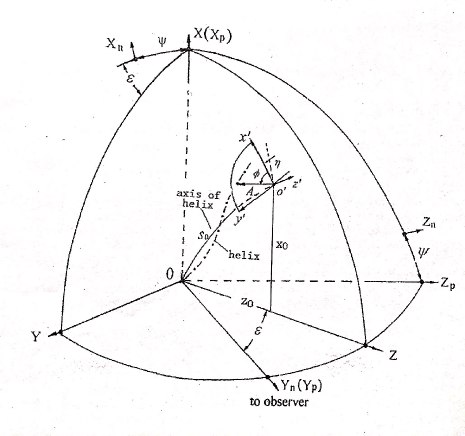
Figure 1: Geometry of the precessing jet-nozzle scenario for 3C345. The jet-axis is defined in the $(X,Z)$-plane by parameters ($\epsilon$, $\psi$) and function $\it{x_{0}(z_{0})}$. The common helical trajectory pattern is defined by functions A(Z) and $\phi$(Z) given in Section 2.3 (Figure 2). Because $\epsilon$ is very small, the change in $\psi$ indicates a rotation around the line of sight.

2 The precessing jet nozzle scenario with a precessing common helical trajectory pattern

The precessing jet-nozzle scenario has been previously described (cf. Qian 2022a , 2022b , Qi23 (2023); Qian et al. Qi09 (2009), 1991a ) in detail for investigating the VLBI-kinematics of superluminal components on parsec scales in the QSO 3C345. The formulism of its geometry is recaptulated as follows.
A special geometry consisting of four coordinate systems is shown in Figure 1. We assume that the superluminal components move along helical trajectories around the curved jet axis (i.e., the axis of the helix).
We use coordinate system ($X_{n},Y_{n},Z_{n}$) to define the plane of the sky ($X_{n},Z_{n}$) and the direction of observer ($Y_{n}$), with $X_{n}$-axis pointing toward the negative right ascension and $Z_{n}$-axis toward the north pole.
The coordinate system ($X,Y,Z$) is used to locate the curved jet-axis in the plane ($X,Z$), where $\epsilon$ represents the angle between $Z$-axis and $Y_{n}$-axis and $\psi$ the angle between $X$-axis and $X_{n}$-axis. Thus parameters $\epsilon$ and $\psi$ are used to define the plane where the jet-axis locates relative to the coordinate system ($X_{n},Y_{n},Z_{n}$).
We use coordinate system (${\it{x}}^{\prime}$,${\it{y}}^{\prime}$,${\it{z}}^{\prime}$) along the jet-axis to define the helical trajectory pattern for a knot, introducing parameters $A(s_{0})$ (amplitude) and $\phi(s_{0})$ (phase), where $s_{0}$ represents the arc-length along the axis of helix (or curved jet-axis). ${\it{z}}^{\prime}$-axis is along the tangent of the axis of helix. ${\it{y}}^{\prime}$-axis is parallel to the $Y$-axis and $\eta$ is the angle between ${\it{x}}^{\prime}$-axis and $X$-axis (see Figure 1).

2.1 Expressions for defining the jet axis

In general we assume that the jet-axis can be defined by a function $x_{0}(z_{0})$ in the $(X,Z)$-plane as follows.

$${x_{0}}=p({z_{0}}){{z_{0}}^{\zeta}}$$ (1)

where

$$p({z_{0}})={p_{1}}+{p_{2}}[1+\exp(\frac{{z_{t}}-{z_{0}}}{{z_{m}}})]^{-1}$$ (2)

$\zeta$, $p_{1}$, $p_{2}$, $z_{t}$ and $z_{m}$ are constants. The exponential term is devised for describing the jet-axis gradually curving toward the north, as the trajectory of knot C4 shows on large-scales.

$${s_{0}}=\int_{0}^{z_{0}}{\sqrt{1+(\frac{d{x_{0}}}{d{z_{0}}})^{2}}}{d{z_{0}}}$$ (3)

Therefore, the helical trajectory of a knot can be described in the (X,Y,Z) system as follows.

2.2 Formulas for calculation of kinematic parameters

$$X({s_{0}})=A({s_{0}}){\cos{\phi({s_{0}})}}{\cos{\eta({s_{0}})}}+{x_{0}}$$ (4)

$$Y({s_{0}})=A({s_{0}}){\sin{\phi({s_{0}})}}$$ (5)

$$Z({s_{0}})=-A({s_{0}}){\cos{\phi({s_{0}})}}{\sin{\eta({s_{0}})}}+{z_{0}}$$ (6)

where $\tan{\eta({s_{0}})}$=$\frac{d{x_{0}}}{d{z_{0}}}$. The projection of the helical trajectory on the sky-plane (or the apparent trajectory) is represented by

$${X_{n}}={X_{p}}{\cos{\psi}}-{Z_{p}}{\sin{\psi}}$$ (7)

$${Z_{n}}={X_{p}}{\sin{\psi}}+{Z_{p}}{\cos{\psi}}$$ (8)

where

$${X_{p}}=X({s_{0}})$$ (9)

$${Z_{p}}={Z({s_{0}})}{\sin{\epsilon}}-{Y({s_{0}})}{\cos{\epsilon}}$$ (10)

(All coordinates and amplitude (A) are measured in units of mas). Introducing the functions

$${\Delta}=\arctan[(\frac{dX}{dZ})^{2}+(\frac{dY}{dZ})^{2}]^{-\frac{1}{2}}$$ (11)

$${{\Delta}_{p}}=\arctan(\frac{dY}{dZ})$$ (12)

$${{\Delta}_{s}}=\arccos[(\frac{dX}{d{s_{0}}})^{2}+(\frac{dY}{d{s_{0}}})^{2}+(\frac{dZ}{d{s_{0}}})^{2}]^{-\frac{1}{2}}$$ (13)

we can then calculate the viewing angle $\theta$, apparent transverse velocity ${\beta}_{a}$, Doppler factor $\delta$ and the elapsed time T, at which the knot reaches distance $z_{0}$ as follows:

$${\theta}=\arccos[{\cos{\epsilon}}(\cos{\Delta}+\sin{\epsilon}\tan{{\Delta}_{p}})]$$ (14)

$${\Gamma}=(1-{\beta}^{2})^{-\frac{1}{2}}$$ (15)

$${\delta}=[{\Gamma}(1-{\beta}{\cos{\theta}})]^{-1}$$ (16)

$${{\beta}_{app}}={{\beta}{\sin{\theta}}/(1-{\beta}{\cos{\theta}})}$$ (17)

$$T=\int^{{s_{0}}}_{0}{\frac{(1+z)}{{\Gamma\delta}{v}{\cos{{\Delta}_{s}}}}}{d{s_{0}}}$$ (18)

2.3 Precessing common helical trajectory pattern

The amplitude and phase of the precessing comm trajectory pattern (helical trajectory pattern) for superluminal knots are defined as follows.

$${A({Z})}={{A_{0}}[\sin({\pi}{Z}/{Z_{1}})]^{1/2}}$$ (19)

$${\phi}({Z})={{\phi}_{0}}-{({Z}/{Z_{2}})^{1/2}}$$ (20)

$A_{0}$ represents the amplitude coefficient of the common helical trajectory pattern and ${\phi}_{0}$ is the precession phase of an individual knot, which is related to its ejection time $t_{0}$:

$${\phi_{0}}=4.28+\frac{2\pi}{T_{0}}({t_{0}}-1979.0)$$ (21)

where $T_{0}$=7.30 yr–precession period of the jet-nozzle.

2.4 Adopted values for the precessing jet nozzle scenario

As shown above, the precessing common helical trajectory which the superluminal components follow is defined by parameters ($\epsilon$, $\psi$) , and formulas (1)-(2) and (19)-(21) and the corresponding parameters in them. The following values are adopted:

$\epsilon$=0.0349 rad=$2^{\circ}$; $\psi$=0.125 rad=$7.16^{\circ}$; $\zeta$=2.0, $p_{1}$=0; $p_{2}$=1.34$\times{10^{-4}}$; $z_{t}$=66 mas; $z_{m}$=6 mas; $A_{0}$=0.605 mas, $Z_{1}$=396 mas and $Z_{2}$=3.58 mas.

We apply the concordant cosmological model (Spergel et al. Sp03 (2003), Hogg Hog99 (1999)) with $\Omega_{\lambda}$=0.73, $\Omega_{m}$=0.27 and $H_{0}$=71 km$s^{-1}$$Mpc^{-1}$. Thus the luminosity distance of 3C345 is $D_{L}$=3.49 Gpc, angular-diameter distance $D_{a}$=1.37 Gpc, 1mas=6.65 pc and 1mas/yr=34.6 c. 1 c is equivalent to an angular speed 0.046 mas/yr.

2.5 Basic equations for Doppler boosting effct and flux evolution

In order to investigate the relation between the flux evolution of superluminal components and their Doppler boosting effect during their accelerated/decelerated motion along helical trajectories, the observed flux density of superluminal components can be described as follows.

$${S_{obs}}(\nu,t)={S_{int}}(\nu,t){\times}{\delta(t)}^{3+\alpha(\nu,t)}$$ (22)

$S_{obs}(\nu,t)$$\propto{\nu^{-\alpha(\nu,t)}}$–the observed flux density and $\alpha(\nu,t)$–spectral index at the observing frequency $\nu$, $S_{int}(\nu,t)$– intrinsic flux density, $\delta(t)$–Doppler factor. Note that both variations in intrinsic flux and spectral index with time and frequency can give rise to variations in the observed flux densities.
We also use normalized flux density ${S_{obs,N}}(\nu,t)$ which is defined as

$${S_{obs,N}}(\nu,t)={S_{obs}}(\nu,t)/{S_{obs,max}}$$ (23)

$S_{obs,max}$–the observed maximum flux density.
In the precessing nozzle scenario the Doppler factor $\delta(t)$ of superluminal knots depends on their motion along helical trajectories which are produced by the precessing common trajectory at corresponding precession phases (or ejection epochs). As shown in the previous works, the kinematics of the superluminal components can well be model-fitted, and their bulk Lorentz factor $\Gamma(t)$ and Doppler factor $\delta(t)$ as continuous functions of time can be derived, which can be used to investigate the relation between the Doppler boosting effect and their flux evolution.

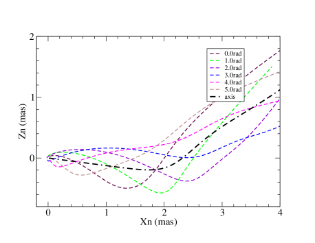
Figure 2: Apparent distribution of the precessing common helical trajectory for different precession phases of the superluminal components in 3C345: $\phi_{0}$=0.0, 1.0, 2.0, 3.0, 4.0 and 5.0 rad, showing the apparent curvature of trajectories around the apparent jet-axis (black dashed line).

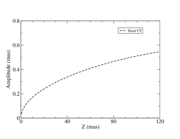
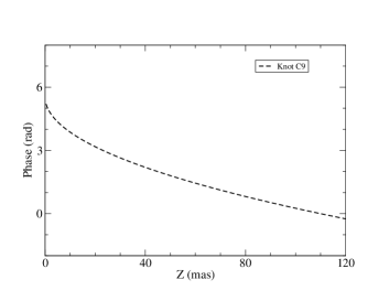
Figure 3: Knot C9: The amplitude A(Z) and phase $\phi$(Z) defining the precessing common helical trajectory pattern (equations (19) and (20) in the text.

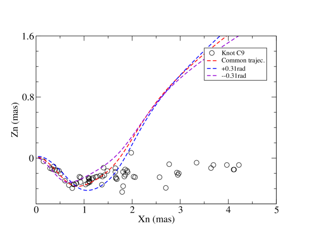
Figure 4: Knot C9: model-fitting of the observed trajectory in terms of the precessing common helical trajectory pattern (red line with $\phi_{0}$=4.28 rad; within $X_{n}{\leq}$1.2 mas). The blue and violent curves with $\phi_{0}$=4.28$\pm$0.31 rad show the uncertainty range of $\pm$5% of the precession period $T_{0}$ (=7.3 yr). Beyond $X_{n}$=1.2 mas its trajectory started to deviate northward from the precessing common pattern, following its own individual track.

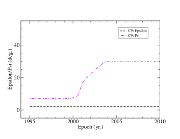
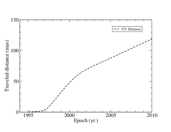
Figure 5: Knot C9. The modeled parameters $\epsilon(t)$ and $\psi(t)$ (left panel) and the travelled distance Z(t) along the Z-axis (right panel), showing $\epsilon$=const.=$2^{\circ}$ and $\psi$=$7.16^{\circ}$ before 1999.80 (corresponding $r_{n}{\leq}$1.25 mas, $X_{n}{\leq}$1.21 mas and traveled distance Z$\leq$44.8 pc), when it moved along the precessing common pattern (in its inner trajectory-region). After 1999.80 $\psi$ increased and it started to move along its own individual track (in its outer trajectory-region) extending to the travelled distance $\sim$104 mas$\sim$692 pc; corresponding core distance $r_{n}{\sim}$4.1 mas (see Fig.6).

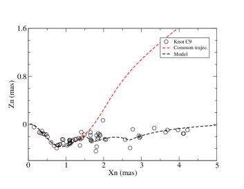
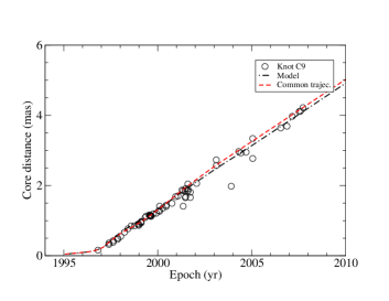
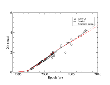
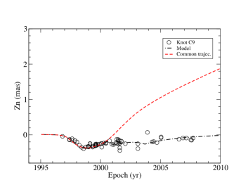
Figure 6: Knot C9: Model-fitting of its whole kinematics extending to core distance $r_{n}{\sim}$4.2 mas: whole trajectory $Z_{n}(X_{n})$, core distance $r_{n}$(t), coordinates $X_{n}$(t) and $Z_{n}$(t). The transition between the precessing common helical trajectory pattern and its own individual track occurred at core distance $r_{n}{\simeq}$1.25 mas (or $X_{n}{\simeq}$1.21 mas; 1999.80). It can be seen that the observed trajectory deviates prominently from the precessing common trajectory mainly in the direction of $Z_{n}$ (declination).

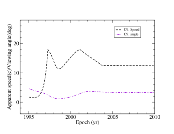
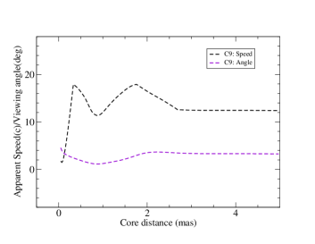
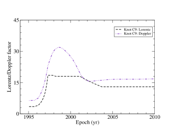
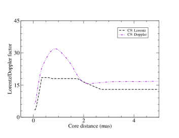
Figure 7: Knot C9: The model-derived appparent speed $\beta_{app}$/viewing angle $\theta$ as functions of time and core distance (upper panels), and the model-derived bulk Lorentz factor $\Gamma$/Doppler factor $\delta$ (bottom panels) which are used to model-fitting of its observed flux evolution. During 1997–2001 ($r_{n}{\sim}$0.33–1.75 mas) knot C9 underwent an apparent acceleration-deceleration-reacceleration process induced by the change in its viewing angle, creating a smooth broad profile of its Doppler factor which is well coincident with the light curves measured at 15-22-43 GHz. (see Table 1 and Figure 8).

Table 1: Kont C9. The model-derived kinematic parameters for five epochs during the period of its acceleration/deceleration and Doppler boosting (Figures 7 and 8): t (epoch), $r_{n}$ (core distance in mas), $X_{n}$ (coordinate in mas), $\beta_{app}$ (apparent speed in c), $\Gamma$ (bulk Lorentz factor), $\delta$ (Doppler factor), $\theta$ (viewing angle in deg.), $Z_{m}$ (traveled distance in mas), $Z_{p}$ (traveled distance in pc). The maximum Doppler factor ($\delta_{max}$=31.9 at 1998.63) is coincident with the minimum viewing angle $\theta_{min}$=$1.14^{\circ}$ and minimum apparent speed $\beta_{app,min}$=11.4c.

t	$r_{n}$	$X_{n}$	$\beta_{app}$	$\Gamma$	$\delta$	$\theta$	$Z_{m}$	$Z_{p}$
1996.96	0.21	0.20	8.1	10.1	16.0	2.91	3.20	21.3
1997.30	0.33	0.32	17.9	18.5	23.0	2.42	6.00	39.9
1998.63	0.87	0.80	11.4	18.0	31.9	1.14	26.4	175.6
2001.13	1.76	1.74	17.9	18.0	19.4	2.94	61.6	409.6
2003.83	2.73	2.72	12.6	13.0	16.2	3.44	80.8	537.3

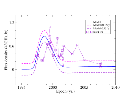
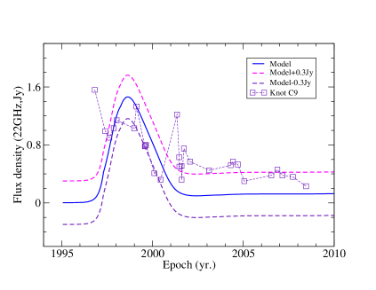
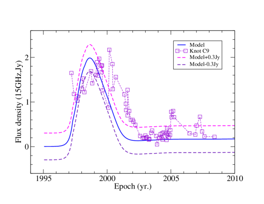
Figure 8: Knot C9: model fitting of the flux evolution measured at 43, 22 and 15 GHz. The model-derived Doppler boosting profiles (black lines), which are associated with the change in its viewing angle, can well fit the light curves, especially at 15 GHz (lower panel). Its intrinsic variations in flux densitty and spectral index give rise to the fluctuations with shorter timescales at different times. The blue and violent lines show the range of these fluctuatons. The intrinsic base-level flux densities at 15, 22 and 43 GHz are 3.83, 2.82 and 1.65$\mu$Jy and spectral index $\alpha$=0.80. Maximum Doppler factor $\delta_{max}$=31.9 at 1998.63.

3 Interpretation of kinematics and flux evolution for knot C9

As show in the previous paper (Qian 2022b ), the flux evolution associated with its Doppler boosting effect is very important and encourages the application of our precessing nozzle scenario to study the phenomena in 3C345 and other blazars. Knot C9 was a typical and exceptionally instructive example of applying the scenario for a satisfying interpretation of its VLBI-kinematics and flux evolution. Here we recaptulate the main results obtained in Qian (2022a , 2022b ) and supplement some new results on its flux evolution and spectral features. All the results for model-fitting of its kinematics and flux evolution are shown in Figures 4–8.

3.1 Model-fits to the kinematics of knot C9

The results of model-fitting of its kinematics can be described as follows.
(1) In the precessing jet-nozzle scenario its precession phase and ejection epoch are adopted as $\phi_{0}$=5.54+4$\pi$ and $t_{0}$=1995.06. The amplitude and phase of its helical trajectory are shown in Figure 3 (see equations (19) and (20)).
(2) For knot C9 the parameters $\epsilon$ and $\psi$ as function of time are modeled as shown in Figure 5 (left), indicating that knot C9 moved along the precessing common trajectory before 1999.94. After 1999.94 parameter $\psi$ started to increase (here $\epsilon$=const.=$2^{\circ}$), and the modeled jet-axis started to deviate from the direction defined in the scenario and knot C9 moved along its own individual track. Thus its precessing common trajectory extends to core distance $r_{n}$=1.25 mas and the corresponding traveled distance $\sim$298 pc (or $\sim$45 mas; see Figure 5 (right) and Table 2).
(3) The curved trajectory observed within $X_{n}$$\sim$1.5 mas for C9 is the projection of its precessing helical common trajectory, which fits the observational data very well as shown in Figure 4. Beyond $X_{n}$$\sim$1.5 mas the observed trajectory clearly deviated from the precessing helical common trajectory and knot C9 moved along its own individual trajectory. In the Figure two trajectories defined by $\phi_{0}$=5.54$\pm$0.31 rad are also shown, demonstrating that within $X_{n}\sim$1.5 mas the observed trajectory section was very accurately fitted by the processing common helical trajectory (in the range of $\pm$5% of the precession period, or $\pm$0.36 yr.).
(4) In Figure 6 the model-fitting results of its entire kinematics (during 1996–2008; or in the core-distance range $r_{n}$=[0–4.2 mas]) are presented: the entire trajectory $Z_{n}(X_{n})$, core separation $r_{n}(t)$, coordinates $X_{n}(t)$ and $Z_{n}(t)$. It can be seen that all these properties are very well fitted by the model, but the precessing common trajectory only applies to the inner trajectory section within $r_{n}$$\stackrel{{\scriptstyle<}}{{{}_{\sim}}}$1.25 mas. The deviation of its outer track occurred mainly in the direction of $Z_{n}$ (declination).
(5) The model-derived apparent velocity $\beta_{app}(t)$, viewing angle $\theta(t)$, bulk Lorentz factor $\Gamma(t)$ and Doppler factor $\delta(t)$ are shown as functions of both time and core distance in Figure 7. It accelerates to $\beta_{app}{\sim}$18c near the core ($r_{n}{\sim}$0.33 mas; 1997.3) and decelerates to $\sim$11.4c at $r_{n}{\sim}$0.87 mas (1998.6). Then it re-accelerates to 18.0 c at $r_{n}{\sim}$1.76 mas (2001.13) and re-decelerates to 12.6 c at $r_{n}{\sim}$2.73 mas (2003.83). [Note: within $r_{n}{\sim}$1.25 mas (or before 1999.80, the observed trajectory of C9 is well fitted by the precessing common helical trajectory of our scenario]. It worths emphasizing that our model fitting results on the change in apparent speed associated with the twisted trajectory are very well consistent with the measurments by Jorstad et al. (Jo05 (2005)).
(6) As shown in Figure 7 the model-derived Doppler factor profile is closely related to the change in apparent speed $\beta_{app}$. The maximum Doppler factor (31.9 at 1998.63) is coincident with the minimum apparent speed (11.4 c) and minimum viewing angle ($\theta$=$1.14^{\circ}$). That is, the Doppler factor profile is closely related to its motion along the common helical trajectory (mainly during 1997–2000; see Table 1).

3.2 Doppler boosting effect and flux evolution of knot C9

The model-derived Doppler factor $\delta(t)$ as a continuous function of time is shown in Figure 7 has a broad smooth bump structure during 1997–2002, providing a distinctly smooth Doppler boosting profile to study the Doppler boosting effect in the flux density variations observed in knot C9. This is rare and extremely valuable opportunity to test our precessing nozzle scenario: whether our scenario is able to fully interprete the entire phenomena measured by VLBI observations, including both kinematics and radiation properties.
The light curves measured at 15GHz, 22GHz and 43GHz are well fitted by the derived Doppler boosting effect as shown in Figure 8. The model-derived broad (1997–2001) Doppler boosting profiles ${S_{int}}[\delta(t)]^{3+\alpha}$ are well coincident with the observed light curves. But due to its intrinsic flux density variations with shorter timescales the data points fluctuate up and down, deviating from the Doppler boosting profiles. Moreover, there are more individual flux peaks with short time-scales at different times, for example, in the 15GHz light curve at 1997.20, 2000.17, 2001.60, 2005.17 and 2007.27. These short timescale variations reveal the variations in their spectral index in the spectral range (15 GHz–22 GHz–43 GHz). For example, at 1998.23 and 1998.41, the observed 43 GHz flux densities are especially low ($\alpha$(15-43GHz)$\simeq$1.6–1.8), implying the intrinsic variations show spectral steepening at this frequency. In contrast, the observed spectral index $\alpha$(15-22GHz)${\simeq}$–1.99, implying an inverted spectrum in the (15-22GHz) waveband. Thus in order to explain the flux evolution of knot C9 both Doppler boosting effect and intirnsic variations should be taken into account.
Here we would like to emphasize the two points: (1) The model which we used for fitting the kinematic behavior of knot C9 is able to derive its bulk Lorentz factor, viewing angle and Doppler factor as continuous functions of time and predict its Doppler boosting profile $[\delta(t)/\delta_{max}]^{3+\alpha}$. Thus the full coincidence of its measured light curves with the Doppler boosting profiles (both in timescale and pattern) may be regarded as a sound argument for the validity of the precessing nozzle scenario with a precessing common helical trajectory pattern; (2) The coincidence of the timescales of the light curves and that of the Doppler boosting profiles also has distinctive implications, showing that the measured variability timescales are compressed by the light-travel-time effects. These effects are effective for both the Doppler boosting profiles (with varying Doppler factors) and the superposed shorter timescale intrinsic variations (with constant Doppler factors) in the case of superluminal components. Similarly, in the traveling relativistic shocks propagating in turbulent jets, the light-travel-time effects are also significant for understanding the rapid (e.g. intraday) variability observed at centimeter wavelengths in blazars, solving the problem of extremely high brightness tempratures and the requirement of extremely high bulk Lorentz factors ($\Gamma$$\stackrel{{\scriptstyle>}}{{{}_{\sim}}}$100). Discussions on the application of the light-travel-time effect are referred to: Quirrenbach et al. Qu89 (1989), Qu91 (1991), Qu92 (1992), Qian et al. 1991c , 1996a , Kraus et al. Kr99 (1999), Kr03 (2003), Krichbaum et al. Kri91 (1991), Kri02 (2002), Begelman et al. Be94 (1994), Standke et al. St96 (1996), Marscher Ma93 (1993), Marscher et al. Ma92 (1992), Gabuzda et al. Ga99 (1999), Ga98 (1998), Kochanev & Gabuzda Ko98 (1998), Wagner et al. Wa93 (1993), Witzel et al. Wi88 (1988).

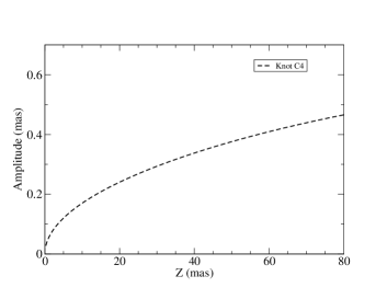
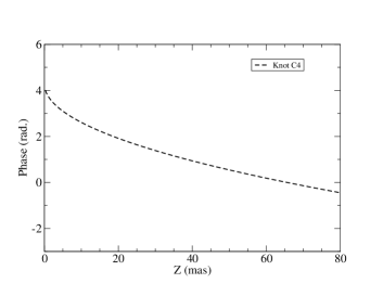
Figure 9: Knot C4: The amplitude A(Z) and phase $\phi$ defining the precessing common helical trajectory pattern with $\phi_{0}$=4.28 rad and ejection time $t_{0}$=1979.0.

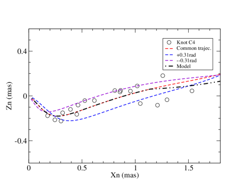
Figure 10: Knot C4: model-fitting of its inner track by the precessing common helical trajectory (the red line) within $X_{n}{\leq}$1.14 mas (corresponding traveled distance Z=40.0 mas or 266.0ṗc). The blue and violent lines indicate the uncertainty range $\pm$5% ($\pm$0.31 rad) of the precession period. The black dashed line indicates the model-fitting of the whole trajectory.

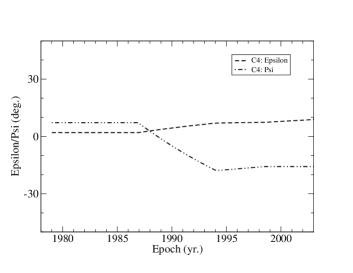
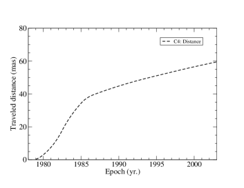
Figure 11: Knot C4. Left panel: functions $\epsilon$(t) and $\psi$(t) defining the jet-axis. Before 1986.91 (corresponding core distance $r_{n}{\leq}$1.14 mas) $\epsilon$=$2^{\circ}$ and $\psi$=$7.16^{\circ}$ knot C4 moved along the precessing common helical traejctory pattern. After 1986.91 (or $r_{n}{>}$1.14 mas) both $\epsilon$ and $\psi$ changed and knot C4 moved along its own individual track. Its traveled distance Z(t) is shown in the right panel.

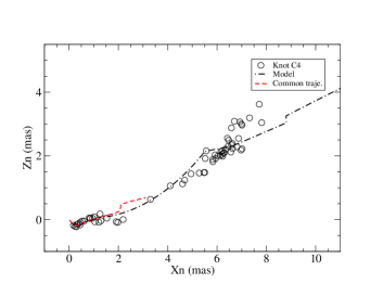
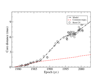
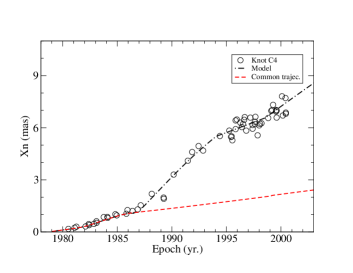
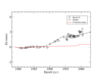
Figure 12: Knot C4: model-fitting of the whole trajectory $Z_{n}(X_{n})$, core distance $r_{n}(t)$, coordinates $X_{n}(t)$ and $Z_{n}(t)$. The transition between the precessing common track and its own individual track occurred at $X_{n}$=1.14 mas (corresponding traveled distance Z=40.0 mas=266.0 pc.). Its whole trajectory extends to core distance $r_{n}{\sim}$7.53 mas ($X_{n}{\sim}$7.11 mas; corresponding traveled distance Z=56.3 mas=374.2 pc). The red lines indicate the precessing common track, while the black lines indicate the model-fitting of the whole track.

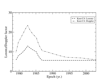
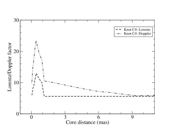
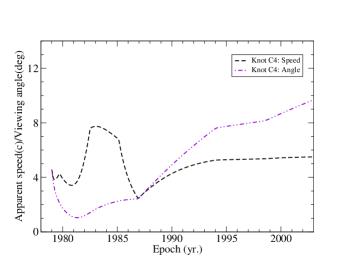
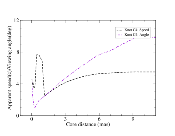
Figure 13: Knot C4: the model-derived bulk Lorentz factor $\Gamma(t)$/Doppler factor $\delta(t)$ and apparent speed $\beta_{app}(t)$/viewing angle $\theta(t)$ as continuous functions of time (t) (left panels) and core distance $r_{n}$ (right panels).

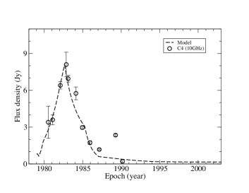
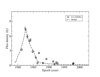
Figure 14: Knot C4: The light curves measured at 10 GHz and 22 GHz are well fitted by the Doppler boosting profiles.

Table 2: Parameters of the precessing common trajectory fitted to the thirteen knots (C9 and C4; C5–C7, C10–C14, C22 and C23): $\phi_{0}$ (precession phase,rad), $t_{0}$ (ejection epoch), $r_{n,com}$ (core separation or the extension of the common trajectory from the core), $Z_{com,mas}$ (the corresponding travelled distance in mas) and $Z_{com,pc}$ (the corresponding traveled distance in pc). References: this paper (C4 and C9); Qian 2022b (C5, C10 and C22); Qian 2022a (C6, C7, C11–C14, C23).

Knot	$\phi_{0}$	$t_{0}$	$r_{n,com}$	$Z_{com,mas}$	$Z_{com,pc}$
C9	5.54+4$\pi$	1995.06	1.25	44.8	298
C4	4.28	1979.00	1.14	40.0	266
C5	5.83	1980.80	1.25	44.8	298
C6	5.74+2$\pi$	1987.99	0.40	7.5	49.7
C7	6.14+2$\pi$	1988.46	0.70	14.9	99.3
C10	6.14+4$\pi$	1995.76	0.35	6.13	40.8
C11	5.88+4$\pi$	1995.46	0.75	15.7	104
C12	6.30+4$\pi$	1995.95	0.50	9.7	64.3
C13	6.50+4$\pi$	1996.18	0.70	14.3	95.3
C14	3.16+6$\pi$	1999.61	0.50	18.8	125
C22	5.28+8$\pi$	2009.36	0.20	3.12	20.7
C23	5.20+8$\pi$	2009.27	0.20	3.4	22.6

4 Interpretation of kinematics and flux evolution for knot C4

The precessing common trajectory of knot C4 was observed to extend to core distance $r_{n}$=1.14 mas (corresponding to traveled distance Z=40 mas=266 pc). Thus it is a distinct component in 3C345 having the second longest extension of precessing common trajectory (only second to knot C9). Its whole traejctory observed extends to $r_{n}$=7.53 mas ($X_{n}$=7.11 mas) and the corresponding traveled distance Z=56.3 mas=374.2 pc. Thus the investigation of its kinematics and flux evolution provides another valuable opportunity to examine our precessing nozzle scenario.

4.1 Knot C4: model fitting of the kinematics

The amplitude A(Z) and phase $\phi$(Z) defining its precessing common helical trajectory pattern with $\phi_{0}$=4.28 rad are shown in Figure 9. In Figure 10 the model-fitting of its inner trajectory ($X_{n}{\leq}$1.14 mas, corresponding to epoch 1986.91) by the precessing common trajectory pattern is shown. The blue and violent lines indicate the uncertainty range of $\pm$5% of the precession period ($\pm$0.31 rad or $\pm$0.36 yr). It can be seen that the curvature of its trajectory is well model fitted.
The functions $\epsilon(t)$ and $\psi(t)$ defining the jet-axis for knot C4 and its model-derived traveled distance Z(t) are shown in Figure 11. Before 1986.91 (or core distance $r_{n}{\leq}$1.14 mas, corresponding traveled distance Z=40.0 mas=266.0 pc) $\epsilon$=$2^{\circ}$ and $\psi$=$7.16^{\circ}$, knot C4 moved along the precessing common trajectory pattern. After 1986.91 both $\epsilon$ and $\psi$ changed, knot C4 started to move along its own individual track.
The whole kinematics with its entire trajectory length of 374.2 pc (including trajectory $Z_{n}(X_{n})$, core distance $r_{n}(t)$ and coordinates $X_{n}(t)$ and $Z_{n}(t)$) are all well fitted by the proposed model. (Figure 12).

4.2 Knot C4: Doppler boosting effect and flux evolution

The model-derived bulk Lorentz factor $\Gamma(t)$, Doppler factor $\delta(t)$, apparent speed $\beta_{app}(t)$ and viewing angle $\theta(t)$ as continuous functions of time (t) are shown in Figure 13. During 1980–1987 (or core distance $r_{n}{<}$1.14 mas) model-derived Doppler factor and apparent speed have a bump structure induced by the increase/decrease in Lorentz factor $\Gamma$ and the change in the viewing angle decreasing and then increasing along a concave curve. After 1987 (or $r_{n}{>}$1.14 mas) $\Gamma$=constant and $\delta$ decreases, its apparent acceleration is mainly caused by the increase in its viewing angle.
The flux evolution measured at 10 GHz and 22 GHz can be well explained in terms of its Doppler boosting effect. As shown in Figure 14, the model-derived Doppler boosting profiles well fit the observational data at both frequencies. There are few intrinsic variations which interfere the smooth Doppler profiles.

4.3 A brief summary on the model-fitting results for C4 and C9

The model-fitting results of the kinematics and flux evolution for knots C4 and C9 have significant implications for our precessing jet-nozzle scenario.
(1) Firstly, these results confirm the applicability of the scenario to interpret the VLBI-phenomena observed for the superluminal components in 3C345: their kinematics and flux evolution as a whole. Knots C4 and C9 were well model-fitted to move along the precessing common helical trajectory patterns (with precession phases $\phi_{0}$=4.28 rad and $\phi_{0}$=5.54+4$\pi$, respectively) which extend to core distances of $\sim$1.2 mas or traveled distances of $\sim$300 pc (Table 2). Thus they are the components in 3C345 having the longest extensions of the precessing common helical trajectory pattern, which provides strong arguments for the existence of jet-nozzle precession and precessing common trajectory pattern . In fact, the curvature in their observed trajectories can be well explained in terms of their helical motion within an uncertainty of $\sim{\pm}$5% ($\pm$0.36 yr) of the precession period of 7.3 yr (Figures 4 and 10).
(2) Except knots C4 and C9, the kinematics and flux evolution of knots C5, C10 and C22 have been well model-fitted as a whole in Qian (2022b ) ,indicating their motion in the inner-jet regions following their precessing common helical traejctory patterns. There are more components (C6–C7, C11–C14 and C23) for which their kinematics also have been well expalined (Qian 2022a ), showing their motion in the inner jet regions along the precessing common helical trajectories with their respective precession phases and different extensions $Z_{com,pc}$ in the range of $\sim$20–250 pc (Table 2). Obviously, the flux evolution of these knots can be interpreted in terms of their Doppler boosting effect as well.
(3) For all these superluminal knots mentioned above, both the model-fitting of their kinematics (curved trajectories, coordinates and apparent sppeds) observed in the inner jet regions and the interpretation of their flux evolution in terms of the model-derived Doppler boosting profiles firmly demonstrate the validity of the precessing helical pattern defined by equations (19) and (20) [Figures 2, 4 and 10]. Moreover, the recurrence of the inner-trajectory patterns observed during $\sim$30 years (1980–2009) for knots C5, C6, C9, C11 and C22 [Qian 2022a ] further confirms the existence of precessing common helical trajectory pattern in 3C345.
(4) In this paper we will apply the same scenario as described in Section 2 to interpret both the kinematics and flux evolution of knots C8, C20, C21, B5 and B7, demonstrating that the precessing nozzle scenario is still effective, but their motion follows the precessing common helical trajectory patterns within core distances of $\sim$0.05–0.15 mas. Therefore, a precessing nozzle scenario with a single jet would be applicable to understanding the whole phenomena in 3C345 (both kinematics and emission properties of the superluminal knots).

5 Interpretation of the kinematics and flux evolution for superluminal knots C8, C20, C21, B5 and B7

The kinematics and flux evolution of these five superluminal knots have been investigated in Qian (for knot C8, 2022b ; for knots C20, C21, B5 and B7, Qi23 (2023)). Here we will apply the same precessing nozzle scenario as proposed above (with the same precessing common helical trajectory pattern defined by equations (19) and (20)) to study their kinematic behavior and flux evolution, thus unifying the interpretation of all these superluminal knots’ observed properties in 3C345 in a single-jet scenario.
Since the transitions between their precessing common trajectory pattern and their individual track occurred within core separation $r_{n}$$\stackrel{{\scriptstyle<}}{{{}_{\sim}}}$0.05–0.15 mas, thus their precessing common trajectories were not observed (for knots C20, C21, B5 and B7). Only for knot C8 its transition was observed at 43GHz (Klare et al. 2003), as already investigated before in Qian (2022a ).

6 Knot C8: model-fitting of the kinematics and flux evolution

Its kinematics was already well model-fitted in Qian (2022a ). Here we recaptulate the results and supplement the explanation of its flux evolution in terms of the Doppler boosting effect.

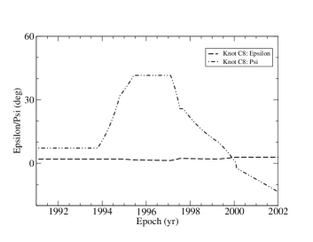
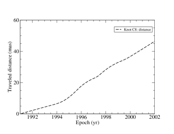
Figure 15: Knot C8 ($\phi_{0}$=2.13+4$\pi$, $t_{0}$=1991.10): Functions $\epsilon(t)$ and $\psi(t)$ (left panel) defining the jet-axis and its traveled distance Z(t). Before 1993.78 (corresponding core distance $r_{n}$=0.14 mas, coordinate $X_{n}$=0.12 mas and traveled distance Z=6.0 mas=39.9 pc), $\epsilon$=$2^{\circ}$ and $\psi$=$7.16^{\circ}$, knot C8 moved along the precessing common helical trajectory pattern. After that $\psi$ increased and knot C8 started to move along its own individual track.

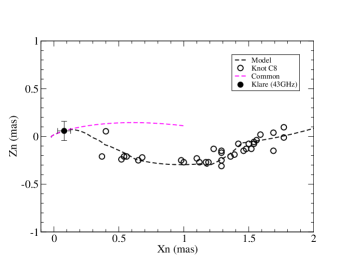
Figure 16: Knot C8: Model-fitting of its kinematics. The datapoint measured at 43GHz in 1992.39 (Klare Kl03 (2003), Klare et al. Kl05 (2005).) indicates it moving along the precessing common helical trajectory (red line; left panel) within $X_{n}{\leq}$0.12 mas. Beyond $X_{n}$=0.12 mas (or after 1993.78) it moved along its own individual track. It can be seen that its whole trajectory $Z_{n}(X_{n})$ (right panel) was well model-fitted. Its core distance $r_{n}(t)$, coordinates $X_{n}(t)$ and $Z_{n}(t)$ are also well fitted by the proposed model.

Figure 17: Knot C8: The model-derived apparent speed $\beta_{app}$(t) and viewing angle $\theta(t)$ are presented in the left panel, and the model-derived bulk Lorentz factor and Doppler factor in the right panel. During 1994–1997 the apparent speed, bulk Lorentz factor and Doppler factor all have a double-peak structure associated with similar changes in its viewing angle. Thus knot C8 underwent a process of acceleration/deceleration/reacceleration/deceleration.

Figure 18: Knot C8: Doppler boosting effect and flux evolution. The model-derived Doppler factor with a double-peak structure leads to the 22 GHz light curve well fitted by the Doppler boosting profile ${S_{int}}{[\delta(t)]^{3+\alpha}}$; $S_{int}$=12.7$\mu$Jy and $\alpha$=1.0.

6.1 Model fits to the kinematics of knot C8

The model-fitting results of kinematics for knot C8 are shown in Figures 15–17. The model-fitted parameters $\epsilon(t)$ and $\psi(t)$ indicate that before 1993.78 knot C8 moved along the precessing common helical trajectory pattern, and after that epoch it moved along its own individual track. The transition occurred at core distance $r_{n}$=0.142 mas (or $X_{n}$=0.122 mas; corresponding traveled distance Z=6.0 mas=39.9 pc). Its whole trajectory $Z_{n}(X_{n})$, core distance $r_{n}(t)$, coordinates $X_{n}(t)$ and $Z_{n}(t)$ are well model-fitted by the precessing nozzle scenario as shown in Figure 16.
During 1994–1997 the model-derived bulk Lorentz factor $\Gamma(t)$, Doppler factor $\delta(t)$ and apparent speed $\beta_{app}(t)$ have a double peak structure associated with a similar change in the viewing angle, demonstrating knot C8’s double acceleration/deleceration process (Figure 17).
We emphasize that the VLBI-observation at 43 GHz for C8 (Klare Kl03 (2003)) is very instructive. In fact, if there were no measurement at 1992.39, we would not be able to recognize that knot C8 moved along its precessing common trajectory pattern within core distance $\sim$0.15 mas. We expected that there may be more superluminal components in 3C345 have similar kinematic behavior, as described below for knots C20, C21, B5 and B7.

6.2 Knot C8: Doppler boosting effect and flux evolution

The model-derived double-peak structure for Doppler factor leads to a Doppler boosting profile ${S_{int}}{[\delta(t)]^{3+\alpha}}$ with a double-peak structure, which nicely explain the observed 22 GHz light cuvre as shown in Figure 18 ($S_{int}$=12.7$\mu$Jy and $\alpha$=1.0).

7 Interpretation of kinematics and flux evolution for knot C20

The kinematics and flux evolution of knot C20 were explained in the framework of double jet scenario in Qian (2022b ), here we apply the single jet scenario as proposed above to study its observed properties. According equation (21) we obtain its precession phase $\phi_{0}$=3.83+8$\pi$, corresponding to its ejection epoch $t_{0}$=2007.68. The model-fitting results are presented in Figures 19–22.

7.1 Knot C20: Model-fitting of the kinematics

The model-derived parameters $\epsilon(t)$ and $\psi(t)$ defining the jet-axis, and its traveled distance Z(t) are shown in Figure 19, revealing that before 2008.23 (corresponding core distance $r_{n}$=0.076 mas, coordinate $X_{n}$=0.041 mas, traveled distance Z=1.20 mas=7.98 pc) $\epsilon$=$2^{\circ}$ and $\psi$=$7.16^{\circ}$, knot C20 moved along the precessing common helical trajectory pattern. After 2008.23 $\psi$ started to decrease and it then moved along its own individual track. This inner precessing common track section is very short and was not observed.
In Figure 20 its whole trajectory $Z_{n}(X_{n})$ (black line, left panel; the red-line indicating the precessing common track), and core distance $r_{n}(t)$, coordinates $X_{n}(t)$ and $Z_{n}(t)$ (right panel) are well model-fitted .
The model-derived bulk Lorentz factor and Doppler factor are presented in Figure 21 (left panel), both showing a single-peak structure. Its apparent speed and viewing angle are shown in the right panel. During 2008–2010.4 its viewing angle varies following a concave curve.

7.2 Knot C20: Doppler boosting effect and flux evolution

The model-derived Doppler factor as a continuous function of time (t) provides a valuable chance to study its flux evolution. As shown in Figure 22, its 43GHz light curve measured is well model-fitted by its Doppler boosting profile (${S_{int}}[\delta(t)]^{3+\alpha}$) (with $S_{int}$=35.7$\mu$Jy, $\alpha$=0.50). Intrinsic variations superposes on it quite prominently.

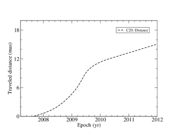
Figure 19: Knot C20: the model-derived parameters $\epsilon(t)$ and $\psi(t)$ defining the jet-axis (left panel) and the traveled distance Z(t). Before 2008.23 $\epsilon$=$2^{\circ}$ and $\psi$=$7.16^{\circ}$ (corresponding core distance $r_{n}$=0.076 mas, $X_{n}$=0.041 mas and traveled distance Z=1.20 mas=7.98 pc), knot C20 moved along the precesssing common helical trajectory pattern, while after that epoch $\psi$ started to decrease and it then moved along its own individual track. Its trajectory-transit occurred near the core and was not observed.

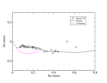
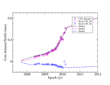
Figure 20: Knot C20. The whole trajectory $Z_{n}(X_{n})$ is well model-fitted by the proposed model (left panel, black line; the red line indicating the precessing common track). The model-fits to the core distance $r_{n}(t)$, coordinates $X_{n}(t)$ and $Z_{n}(t)$ are shown in the right panel.

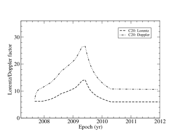
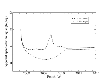
Figure 21: Knot C20. The model-derived bulk Lorentz factor $\Gamma(t)$ and Doppler factor $\delta(t)$ show a broad peak structure during $\sim$2008.4–2010.0 (left panel) associated with the increase in its core distance $r_{n}$ (Fig.20; right panel). Correspondingly, the model-derived viewing angle $\theta(t)$ changes along a concave curve (right panel). The model-derived apparent speed $\beta_{app}(t)$ only shows a short-period peak during $\sim$2009.0–2009.6.

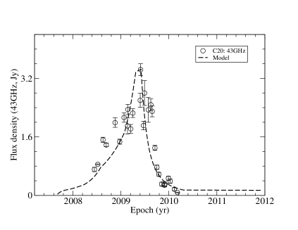
Figure 22: Knot C20. Its 43GHz light curve is well fitted by the model-derived Doppler boosting profile ${S_{int}}[\delta(t)]^{3+\alpha}$ with $S_{int}$=35.7$\mu$Jy and $\alpha$=0.50. Intrinsic variations are prominently superposed.

8 Interpretation of kinematics and flux evolution for knot C21

The model-fitting results of kinematics and flux evolution for knot C21 are shown in Figures 23–26. Its precession phase $\phi_{0}$=3.52+8$\pi$ corresponding to its ejection epoch $t_{0}$=2007.32 (Qian 2022b ).

8.1 Knot C21: model-fitting of the kinematics

The model-derived parameters $\epsilon(t)$ and $\psi(t)$ defining the jet-axis are shown in Figure 23 (left panel) and indicate that before 2008.88 [corresponding core distance $r_{n}$=0.11 mas, coordinate $X_{n}$=0.060 mas, traveled distance Z=3.97 mas=26.4 pc (right panel)], $\epsilon$=$2^{\circ}$ and $\psi$=$7.16^{\circ}$, knot C21 moved along the precessing common helical trajectory pattern, while after 2008.88 $\psi$ started to change and it started to move along its own individual track. Its trajectory-transit occurred near the core and was not observed.
Its whole trajectory $Z_{n}(X_{n})$ was well fitted by the proposed model (Figure 24, left panel; the red line indicating the precessing common trajectory section). The core distance $r_{n}$ and coordinates $X_{n}$ and $Z_{n}$ are well model-fitted (right panel).
The model-derived bulk Lorentz factor $\Gamma(t)$ and Doppler fcator $\delta(t)$ are presented in Figure 25 (left panel), both having a double-peak structure during 2009.0–2010.4. The model-derived apparent speed $\beta_{app}(t)$ also has a double-peak structure, but the second peak is much more prominent.

8.2 Knot C21. Doppler boosting effect and flux evolution

As shown in Figure 26 the doule-peak structure of its 43GHz light curve is very well fitted by the Doppler boosting profile ${S_{int}}[\delta(t)]^{3+\alpha}$ with $S_{int}$=25.6$\mu$Jy and $\alpha$=0.50.

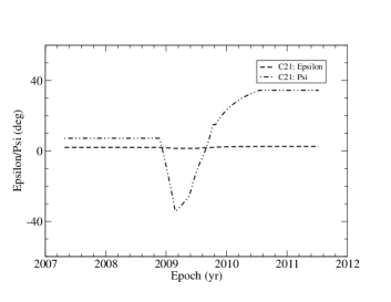
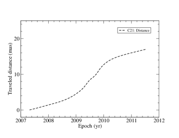
Figure 23: Knot C21. The model-derived curves of parameters $\epsilon$ and $\psi$ (left panel) indicate that $\epsilon$=$2^{\circ}$ and $\psi$=$7.16^{\circ}$ before 2008.88 [corresponding core distance $r_{n}$=0.11 mas, coordinate $X_{n}$=0.060 mas, traveled distance Z=3.97 mas=26.4 pc], knot C21 moved along the precessing common helical trajectory pattern, while after 2008.88 $\psi$ decreases and it started to move along its own individual track.

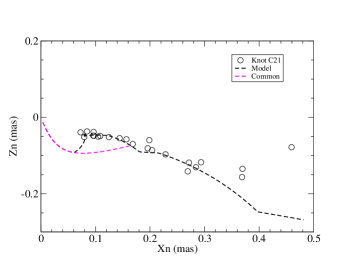
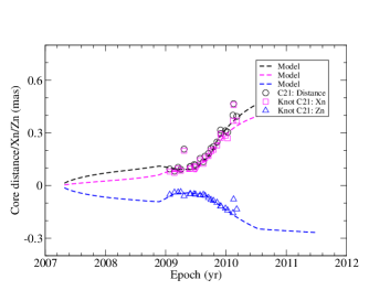
Figure 24: Knot C21. Its whole trajectory $Z_{n}(X_{n})$ (left panel), core distance $r_{n}$ and coordinates $X_{n}$ and $Z_{n}$ (right panel) are well fitted by the proposed model. The red line indicates the precessing common trajectory, showing the modeled trajectory-transit at $X_{n}$=0.06 mas.

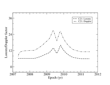
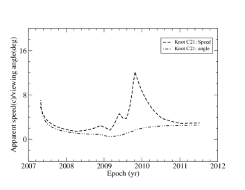
Figure 25: Knot C21. The model-derived bulk Lorentz factor $\Gamma(t)$ and Doppler factor $\delta(t)$ having a double-peak structure during 2009.0–2010.4 (left panel). The model-derived apparent speed $\beta_{app}(t)$ also shows a double-peak structure, but the second one is much more prominent. The viewing angle $\theta(t)$ varies along a concave curve.

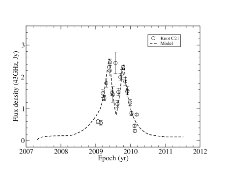
Figure 26: Knot C21. The 43 GHz light curve is very well fitted by the model-derived Doppler boosting profile ${S_{int}}[\delta(t)]^{3+\alpha}$ with $S_{int}$=25.6$\mu$Jy and $\alpha$=0.5.

9 Interpretation of kinematics and flux evolkution for knot B5

The model-fitting results of the knematics and flux evolution for knot B5 are presented in Figures 27–30. Its precession phase $\phi_{0}$=6.24+8$\pi$ corresponding to its ejection epoch $t_{0}$=2010.48 (Table 3; Qian 2022b ).

9.1 Model fits to the kinematics of knot B5

The model-derived parameters $\epsilon(t)$ and $\psi(t)$ defining the jet-axis are shown in Figure 27 (left panel), which indicates that its trajectory-transit occurred at 2010.66. Before 2010.66 [corresponding core distance $r_{n}$=0.039 mas, coordinate $X_{n}$=0.028 mas, traveled distance Z=0.36 mas=2.39 pc (right panel)], $\epsilon$=$2^{\circ}$ and $\psi$=$7.16^{\circ}$, knot B5 moved along the precessing common helical trajectory, while after 2010.66 $\psi$ started to increase and it started to move along its own individual track.
Its whole trajectory is well fitted by the proposed model as shown in Figure 28 (left panel; the red-line indicating the precessing common trajectory with its trajectory-transit at $X_{n}$=0.039 mas). The core distance $r_{n}$, coordinates $X_{n}$ and $Z_{n}$ are also very well model-fitted (right panel).
The model-derived bulk Lorentz factor $\Gamma(t)$ and Doppler factor $\delta(t)$ are shown in Figure 29 (left panel), revealing a double-peak structure. Correspondingly, the model-derived apparent speed $\beta_{app}(t)$ (right panel) also has a similar double-peak structure. Its viewing angle varied along a concave curve (during the first peak) and then along a convex curve (during the second peak).

9.2 Knot B5: Doppler boosting effect and flux evolution

Its 43 GHz light curve is well fitted by the model-derived Doppler boosting profile ${S_{int}}[\delta(t)]^{3+\alpha}$ with $S_{int}$=37.0$\mu$Jy and $\alpha$=0.5, as shown in Figure 30. Due to the increase in the viewing angle (along a convex curve) during 2012–2014.5 its second ”flare” only shows low flux variations.

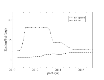
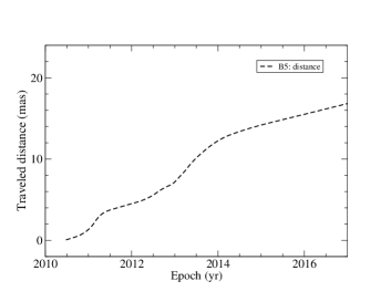
Figure 27: Knot B5. The model-derived parameters $\epsilon(t)$ and $\psi(t)$, indicating the trajectory-transit occurred at 2010.66, when the corresponding core distance $r_{n}$=0.039 mas, coordinate $X_{n}$=0.028 mas, and the traveled distance Z=0.36 mas=2.39 pc (right panel). So, knot B5 moved along the precessing common helical trajectory pattern before 2010.66, while after 2010.66 it started to move along its own individual track.

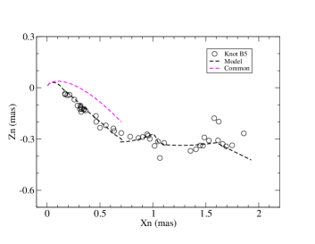
Figure 28: Knot B5. Its whole trajectory $Z_{n}(X_{n})$ is well fitted by the proposed model (black line, left panel; the red-line indicating the precessing common trajectory and the trajectory transit at $X_{n}$=0.028 mas). Its core distance $r_{n}$, coordinates $X_{n}$ and $Z_{n}$ are all well model-fitted (right pane).

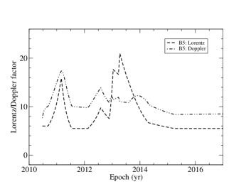
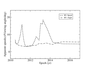
Figure 29: Knot B5. The model-derived bulk Lorentz factor $\Gamma(t)$ and Doppler factor $\delta(t)$ are presented in left panel, both revealing a double-peak structure, but the second peak in Doppler factor is much lower due to the increase in the viewing angle. Correspondingly, the model-derived apparent speed has a similar double structure (right panel). The viewing angle varies along a convex curve, leading to the second peak of the apparent speed much broader than the first one.

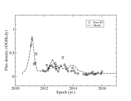
Figure 30: Knot B5. Doppler boosting effect and Flux evolution. Corresponding to the double-peak structure, the model-derived Doppler boosting profile ${S_{int}}[\delta(t)]^{3+\alpha}$ also has a similar double-peak structure and well fits the observed 43 GHz light curve. The second ”Doppler-boosted flare” is much weaker than the first one due to the increase in the viewing angle and the decrease in Doppler factor during 2012.0–2014.5 (Fig.29). $S_{int}$=37.0$\mu$Jy and $\alpha$=0.50.

Table 3: Parameters of the precessing common trajectory for five superluminal knots (C8, C20, C21, B5 and B7): precession phase $\phi_{0}$(rad), ejection epoch $t_{0}$, extension of the precessing common trajectory from the core $r_{n,com}$ (in mas), the corresponding traveled distance $Z_{com,mas}$ (in mas) and $Z_{com,pc}$ (in pc).

Knot	$\phi_{0}$	$t_{0}$	$r_{n,com}$	$Z_{com,mas}$	$Z_{com,pc}$
C8	2.13+4$\pi$	1991.10	0.14	6.0	39.9
C20	3.83+8$\pi$	2007.68	0.076	1.20	7.98
C21	3.52+8$\pi$	2007.32	0.11	3.97	26.4
B5	6.24+8$\pi$	2010.48	0.039	0.36	2.39
B7	0.92+10$\pi$	2011.60	0.14	3.00	20.0

10 Interpretation of kinematics and flux evolution for knot B7

The model-fitting results of the kinematics and flux evolution for knot B7 are shown in Figures 31–34. Its precession phase $\phi_{0}$=0.92 rad+10$\pi$, corresponding to its ejection epoch $t_{0}$=2011.60.

10.1 Model fits to the kinematics for knot B7.

The model-derived parameters $\epsilon(t)$ and $\psi(t)$ defining the jet axis are shown in Figure 31 (left panel), indicating that before 2012.99 $\epsilon$=$2^{\circ}$ and $\psi$=$7.16^{\circ}$, and knot B7 moved along the precessing common helical trajectory pattern [corresponding to core distance $r_{n}{\leq}$0.14 mas, coordinate ${X_{n}}\leq$0.11 mas, traveled distance Z${\leq}$3.0 mas=20.0 pc (right panel)].
Its whole trajectory is well fitted by the proposed model as shown in Figure 32 (left panel), where the red-line indicates the precessing common trajectory and the trajectory-transit at $X_{n}$=0.11 mas. Its core distance $r_{n}$, coordinates $X_{n}$ and $Z_{n}$ are very well model-fitted as shown in the right panel.
The model-derived bulk Lorentz factor $\Gamma(t)$ and Doppler factor $\delta(t)$ as continuous functions of time are shown in Figure 33 (left panel), revealing a single peak structure duirng 2012.5–2014.0. Correspondingly, the model-derived apparent speed $\beta_{app}(t)$ has a similar single peak structure is presented in the right panel. The model-derived viewing angle $\theta(t)$ is almost constant ($\sim$$2.9^{\circ}$–$3.0^{\circ}$) and the peak structures in the Doppler factor and apparent speed are caused by the change in the Lorentz factor only, not due to the change in the viewing angle.

10.2 Knot B7. Doppler boosting effect and flux evolution

As shown in Figure 34 its 43GHz light curve is very well fitted by the Doppler boosting profile ${S_{int}}[\delta(t)]^{3+\alpha}$ without any interference from its intrinsic flux variations. $S_{int}$=101.2$\mu$Jy and $\alpha$=0.50.

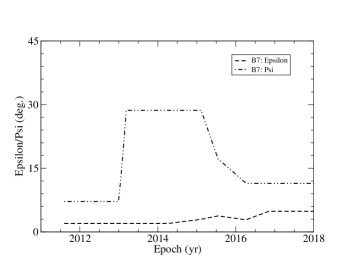
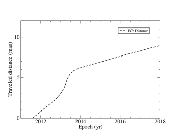
Figure 31: Knot B7. The model-derived curves for parameters $\epsilon(t)$ and $\psi(t)$ defining the jet-axis (left panel), indicating the trajectory transit occurred at 2012.99 [corresponding core distance $r_{n}$=0.14 mas, coordinate $X_{n}$=0.11 mas, traveled distance Z=3.0 mas=20.0 pc (right panel)]. Thus before 2012.99 knot B7 moved along the precessing common helical trajectory pattern, while after 2012.99 it moved along its own individual track.

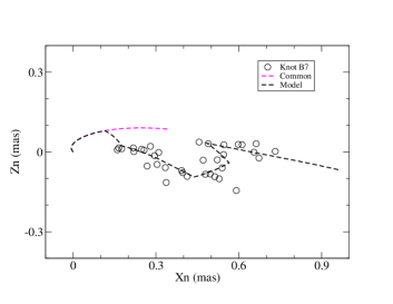
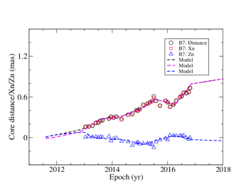
Figure 32: Knot B7. Its whole trajectory $Z_{n}(X_{n})$ is well model-fitted as shown in the left panel. The red-line indicates the precessing common trajectory, demonstrating the trajectory-transit at $X_{n}$=0.11 mas. Its core distance $r_{n}$, coordinates $X_{n}$ and $Z_{n}$ are very well model-fitted (right panel).

Figure 33: Knot B7. The model-derived bulk Lorentz factor $\Gamma(t)$ and Doppler factor $\delta(t)$ are presented in the left panel, showing a single-peak structure during 2012.5–2014.0. The model-derived apparent speed $\beta_{app}(t)$ also has a single-peak structure, while the model-derived viewing angle $\theta(t)$ changes only a little ($\sim$$2.9^{\circ}$–$3.0^{\circ}$) during 2012.5–2014.0. Thus the single peak structure in the apparent speed and Doppler factor are completely due to the acceleration and deceleration of knot B7 (increase and decrease in its bulk Lorentz factor).

Figure 34: Knot B7. The 43 GHz light curve is very well model-fitted by the Doppler boosting profile ${S_{int}}[\delta(t)]^{3+\alpha}$ with $S_{int}$=101.2$\mu$Jy and $\alpha$=0.50.

11 Discussion and Conclusions

In the previous work (Qian 2022a ) we suggested that the superluminal components measured in 3C345 might be divided into two groups: group-A (consisting of 13 knots: C4–C14 and C22-C23) and gorup-B (consisting of 14 knots: C15, C15a, C16–C21, B5–B8 and B11–B12). We interpreted the kinemtics of these knots by assuming that the knots of group-A and group-B are ejected from thier respective jets (jet-A and jet-B), which have the same precession period of 7.3 yr with the same sense. We also assumed that jet-A and jet-B have their individual precessing common helical trajectory patterns along which the knots of group-A and group-B moved respectively in their inner trajectory regions, while in their outer trajectory regions they move along their own individual tracks.
It was shown that the kinematic behavior of all the knots could be well explained in this framework of precessing nozzle scenario with a double-jet structure. And in the work (Qian 2022b ) the flux evolutions of superluminal knots (C4, C5, C9, C10 and C22 of group-A) were well explained in terms of their Doppler boosting effects, which were model-derived from the model-fitting of their kinematics. Similarly, in the work (Qian Qi23 (2023)) the flux density variations of the superluminal knots (C19, C20, C21, B5 and B7 of group-B) were also well explained in terms of their Doppler boosting effects.
Thus, based on the assumption of jet-nozzle precession for blazar 3C345, the precessing nozzle scenario with a double-jet structure as a hypothesized workingframe is useful to understand the kinematics and emission poroperties of the superluminal knots in 3C345.
In this paper we have considered a precessing nozzle scenario with a single jet. We assumed that the superluminal knots of group-B also moved along the same precessing common helical trajectory pattern as the knots of group-A. In this case the trajectory-transits of these knots (C20, C21, B5 and B7) occurred within core distances $r_{n}{<}$0.05–0.15 mas, so only their outer trajectories were observed, and their flux evolution associated with their superluminal motion could be also well explained. We expect that the kinematics and flux evolution of the remained knots (C15, C15a, C16–C19, B6, B8, B11 and B12) could be interpreted as well.
We would like to emphasize that both the scenarios are based on the the possible evidence of the jet (or jets) in 3C345 precssing with a certain period (Klare et al. Kl05 (2005), Qian et al.Qi09 (2009)). Both the precessing nozzle scenarios with a single jet or double-jets have been applied to interpret the kinematics and flux evolution of the superluminal components in 3C345. Higher resolution VLBI-observations deep into the core (within core distance $r_{n}{<}$0.05–0.1 mas) with mm-VLBI and Space-VLBI are required to test them.
Finally, we would emphasize that the explanation of the light curves of superluminal components associated with their superluminal motion in terms of Doppler beaming effects indicates: the light-travel-time effect is important not only for interpreting the apparently superluminal motion of knots observed in blazars, but also for understanding their intrinsic variability, because in these cases the radiation of knots is emitted from the ”emitting elements” distributed in a region with a size of c$\Gamma{\delta}{\Delta{t_{var}}}$ along the line of sight ($\Delta{t_{var}}$–variability time-scale; also cf. Sec.3.2). And continuous injection mechanisms should be taken into account (e.g., Qian 1996b ).

- (1) Artymovicz P., 1998, in: Theory of Black Hole Accretion Disks, ed. M.A. Abramowicz, G. Björnsson, J.E. Pringle, p202
- (2) Babadzhantants M.K., Belokon E.T. & Gamm N.G., 1995, Astronomy Report 39, 393
- (3) Begelman M.C., Rees M.J., Sikora M., 1994, ApJ 429, L57
- (4) Begelman M.C., Blandford R.D. & Rees M.J., 1980, Nature 287, 307
- (5) Biretta J.A., Moore R.L. & Cohen M.H., 1986, ApJ 308, 93
- (6) Blandford R.D., Znajek R.I., 1977, MNRAS 179, 433
- (7) Blandford R.D., Payne D.G., 1982, MNRAS 199, 883
- (8) Gabuzda D.C., Kochenov P. Yu., Cawthorne T.V., 1999, in: ”BL Lac Phenomenon”, ASP Conference Series, Vol. 159, 447, eds. L.O. Takalo & A. Sillanpäpä
- (9) Gabuzda D.C., Kochanov P.Yu., Kollgard R.I., 1998, in: ”IAU Colloquium 164: Radio Emission from Galactic and Extragalactic Compact Sources”, ASP Conference Series, Vol.144, 265, eds. J.A. Zensus, G.B. Taylor & J.M. Wrobel
- (10) Hardee P.E., 1987, ApJ 318, 78
- (11) Hogg D.W., 1999, astro-ph/9905116
- (12) Jorstad S.G., Marscher A.P., Lister M.L., et al., 2005, AJ 130, 1418
- (13) Jorstad S.G., Marscher A.P., Smith P.S., et al. 2013, ApJ 773, 147
- (14) Jorstad S.G., Marscher A.P., Morozova D.A., et al., 2017, ApJ 846, article id. 98
- (15) Klare J., 2003, Quasi-Periodicity in the Parsec-Scale Jet of the Quasar 3C345, PhD Thesis, Rheinische-Friedrich-Wilhelms-Universität Bonn, Bonn, Germany
- (16) Klare J., Zensus J.A., Lobanov A.P., et al., 2005, in ”Future Directions in High Resolution astronomy: The 10th Anniversary of the VLBA”, ASP Conference Series, Vol.340 (eds. J.D. Romney and M.J. Reid), p.40
- (17) Kochanov P.Yu., Gabuzda D.C., 1998, in: ”IAU Colloquium 164: Radio Emission from Galactic and Extragalactic Compact Sources”, ASP Conference Series, Vol.144, p273, eds. J.A. Zensus, G.B. Tayor & J.M. Wrobel
- (18) Krichbaum T.P., Kraus A., Fuhrmann L., et al., 2002, Publ. Astron. Soc. Aust., 19, 14
- (19) Krichbaum T.P., Quirrenbach A., Witzel A., 1991, in: ”Variability of Blazars”, ed. E. Valtaoja & M. Valtonen (Cambridge University Press), 331
- (20) Kraus A., Krichbaum T.P., Wegner R., et al., 2003, A&A 401, 161
- (21) Kraus A., Witzel A., Krichbaum T.P., 1999, New Astron. Rev., 43, 685
- (22) Lobanov A.P. & Roland J., 2005, A&A 431, 831
- (23) Marscher A.P., 1993, in: ”Astrophysical jets”, STScI Symposium Series 6, ed. D. Burgarella, M. Livio, and C. O’Dea (Cambridge U. Press), pp.73–94
- (24) Marscher A.P., Gear W.K., Travis J.P., 1992, in: ”Variability of Blazars”, ed. E. Valtaoja & M. Valtonen (Cambridge Univ. Press), 85
- (25) Meier D.L. & Nakamura M., 2006, in: ”Blazar Variability Workshop II: Entering the GLAST Era”, ed. H.R. Miller, K. Marshall, J.R. Webb & M.F. Aller, ASP Conf. Ser. 350, 195
- (26) Qian S.J., Witzel A., Krichbaum T., et al., 1991a, Acta Astron. Sin. 32, 369 (Chinese Astron. Astrophys. 16, 137 (1992))
- (27) Qian S.J., Krichbaum T.P., Witzel A., et al., 1991b, in: ”High Energy/Astrophysics: Compact Stars and Active Galaxies” (Proceedings of the 3rd Chinese Academy of Sciences and Max-Planck Society workshop held 19-23, October 1990 in Huangshan, China. Edited by Qibin Li, Singapore: World Scientific), p.80
- (28) Qian S.J., Quirrenbach A., Witzel A., et al., 1991c, A&A 241, 15
- (29) Qian S.J., Witzel A., Zensus J.A., et al., 2009, Research in Astron. Astrophys. 9, 137
- (30) Qian S.J., Li X.C., Wegner R., et al., 1996, Chin. Astron. Astrophys. 20, 15
- (31) Qian S.J., 1996b, Chin. Astron. Astrophy. 20, 281
- (32) Qian S.J., 2022a, arXiv:2202.01915
- (33) Qian S.J., 2022b, arXiv:2206.14995
- (34) Qian S.J., 2023, arXiv:2309.00198
- (35) Quirrenbach A., Witzel A., Qian S.J., et al., 1989, A&A 226, L1
- (36) Quirrenbach A., Witzel A., Wagner S., et al., 1991, ApJ 372, L71
- (37) Quirrenbach A., Witzel A., Krichbaum T.P., et al., 1992, A&A 258, 279
- (38) Schinzel F.K., Lobanov A.P., Zensus J.A., 2010, in: ”Accretion and Ejection in AGNs: A Global View”, ASP Conference series, Vol. 427, eds. L. Maraschi, G. Ghisellini, R. Della Ceca and F. Tavecchio, p153
- (39) Schinzel F.K., 2011a, Phyiscs and Kinematics of the Parsec Scale Jet of the Quasar 3C345, PhD Thesis, Universität zu Köln, Germany.
- (40) Shi J.M. & Krolik J.H., 2015, ApJ 807, article id.131
- (41) Spergel D.N., Verde L., Peilis H.V., et al., 2003, ApJS 148, 145
- (42) Standke K.J., Quirrenbach A., Krichbaum T.P., et al., 1996, A&A 306, 27
- (43) Vlahakis N. & Königl A., 2003, ApJ 596, 1080
- (44) Vlahakis N. & Königl A., 2004, ApJ 605, 656
- (45) Wagner S.J., Witzel A., Krichbaum T.P., et al., 1993, A&A 271, 344
- (46) Witzel A., Schalinski C.J., Johnston K.J., et al., 1988, A&A 206, 245
- (47) Zensus, J.A., 1997, ARA&A 35, 607