Deep Coupling Network For Multivariate Time Series Forecasting

Abstract.

Multivariate time series (MTS) forecasting is crucial in many real-world applications. To achieve accurate MTS forecasting, it is essential to simultaneously consider both intra- and inter-series relationships among time series data. However, previous work has typically modeled intra- and inter-series relationships separately and has disregarded multi-order interactions present within and between time series data, which can seriously degrade forecasting accuracy. In this paper, we reexamine intra- and inter-series relationships from the perspective of mutual information and accordingly construct a comprehensive relationship learning mechanism tailored to simultaneously capture the intricate multi-order intra- and inter-series couplings. Based on the mechanism, we propose a novel deep coupling network for MTS forecasting, named DeepCN, which consists of a coupling mechanism dedicated to explicitly exploring the multi-order intra- and inter-series relationships among time series data concurrently, a coupled variable representation module aimed at encoding diverse variable patterns, and an inference module facilitating predictions through one forward step. Extensive experiments conducted on seven real-world datasets demonstrate that our proposed DeepCN achieves superior performance compared with the state-of-the-art baselines.

1. Introduction

Multivariate time series (MTS) forecasting is widely applied in various real-world scenarios, ranging from weather forecasting (Zheng et al., 2015), traffic forecasting (Yu et al., 2018), COVID-19 prediction (Cao et al., 2020), macroeconomics (Li and Chen, 2014), financial analysis (Binkowski et al., 2018), stock prediction (Feng et al., 2019; Li et al., 2019b), to decision making (Borovykh et al., 2017), etc. This broad application has attracted increasing enthusiasm and led to very intensive and diversified MTS research in recent years. In particular, numerous deep learning architectures have been developed to address the challenge of the complex intra- and inter-series relationships among time series (Lim and Zohren, 2021a; Torres et al., 2020).

Previous deep learning work on MTS forecasting can be broadly categorized into two main approaches: sequential models (Zhou et al., 2021; Wu et al., 2021) and GNN-based models (Cao et al., 2020; Bai et al., 2020). Sequential models, including recurrent neural networks (RNNs) (Flunkert et al., 2017; Rangapuram et al., 2018), convolutional neural networks (CNNs) (Borovykh et al., 2017), temporal convolutional networks (TCNs) (Bai et al., 2018), and attention mechanisms (Fan et al., 2019), have been introduced to tackle MTS problems and have achieved good performance, which is attributed to their capability to extract nonlinear intra-series relationships in MTS. However, these models often fall short in effectively capturing inter-series relationships. In contrast, GNN-based models (Cao et al., 2020; Wu et al., 2020) have recently emerged as promising approaches for MTS forecasting with their essential capability to capture the complex inter-series relationships between variables. They predominantly adopt a graph neural network to extract inter-series relationships while incorporating a temporal network to capture intra-series relationships. Unfortunately, the aforementioned methods still exhibit certain limitations in modeling both intra- and inter-series relationships among time series data.

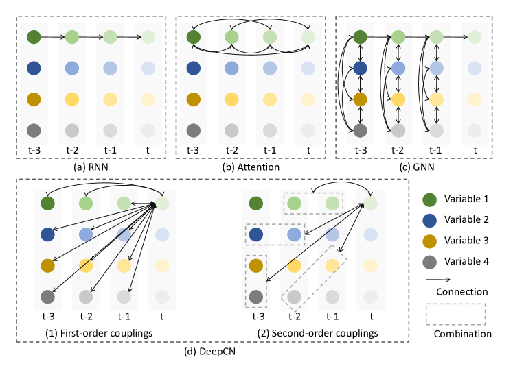
As shown in Fig. 1, the maximum length of the signal traversing path of RNN-based models is $\mathcal{O}(L)$, making it challenging for them to effectively learn intra-series relationships between distant positions (Liu et al., 2022a). Attention-based models (Kitaev et al., 2020; Zhou et al., 2021; Wu et al., 2021) shorten the maximum path to be $\mathcal{O}(1)$ but they ignore inter-series relationships. Recently, GNN-based MTS forecasting models (Yu et al., 2018; Wu et al., 2020, 2019; Bai et al., 2020) have emerged. They combine graph networks to represent inter-series relationships while relying on LSTM or GRU to capture intra-series relationships. However, akin to RNN-based models, GNN-based models also encounter limitations in effectively modeling intra-series relationships. Additionally, they are unable to directly connect different variables at different timestamps, thereby limiting their ability to capture abundant inter-series relationships. Moreover, both sequential models and GNN-based models generally model intra- and inter-series relationships separately, which naturally violates the real-world unified intra-/inter-series relationships, and they also overlook the multi-order interactions embodied within time series data. Consequently, how to model the complex intra- and inter-series relationships calls for a comprehensive analysis. Couplings (Cao, 2015), referring to any relationships or interactions that connect two or more variables, include diverse correlations, dependencies, interactions, and hierarchies. Learning such couplings (Cao, 2015) can explore more comprehensive representations by revealing and embedding various couplings on complex data (Zhu et al., 2022), which has demonstrated success in numerous domains, including recommendation (Jian et al., 2019; Zhang et al., 2022), image source identification (Huang et al., 2018), and financial market analysis (Cao et al., 2015). Motivated by this, we model the complex intra- and inter-series relationships by exploring multi-order couplings as shown in Fig. 1(d).

Figure 1. Illustration of modeling the intra- and inter-series relationships. (a) RNN-based models connect two values at consecutive time steps while ignoring the inter-series relationships. (b) Attention-based models directly link variable values across different time steps but do not consider inter-series relationships. (c) GNN-based models construct a graph to model inter-series relationships at each timestamp and then connect values of adjacent time steps for each variable. (d) Our model DeepCN proposes a coupling mechanism to comprehensively capture intra- and inter-series relationships by leveraging the multi-order couplings of various time lags.

In light of the above discussion, in this paper, we theoretically analyze the relationship modeling within time series data and propose a novel deep coupling network (named DeepCN) for multivariate time series forecasting. Concretely, we revisit the relationships from the perspective of mutual information, and then based on the analysis, we first propose a coupling mechanism to comprehensively model intra- and inter-series relationships explicitly and simultaneously via exploring the diverse and hierarchical couplings in MTS data. Subsequently, we leverage a coupled variable representation module to encode the variable relationship representations since different variables exhibit different patterns. Finally, we utilize an inference module to make predictions by one forward step which can avoid error accumulation. We compare the proposed DeepCN with state-of-the-art baselines on seven real-world datasets. Extensive experimental results show the superiority of DeepCN and demonstrate the effectiveness of the proposed neural architecture and coupling mechanism in DeepCN.

Our main contributions are summarized as follows:

• Compared with previous models, we theoretically revisit intra- and inter-series relationships through the lens of mutual information and construct our model based on the multi-order couplings which can capture more comprehensive information to enhance relationship representations within time series data.

• We design a coupling mechanism to explicitly investigate the complicated intra- and inter-series relationships within time series data simultaneously. The coupling mechanism explores the diverse and hierarchical couplings across various time lags in time series data while maintaining linear computational complexity.

• We propose a DeepCN model for MTS forecasting based on the coupling mechanism which captures complex multivariate relationships to address the relationships modeling issues within MTS data.

• Extensive experimental results on seven real-world datasets show our DeepCN improves an average improvement of 6.2$\%$ on MAE and 7.0$\%$ on RMSE over state-of-the-art baselines. In addition, more empirical analysis on the coupling mechanism further gains insights into the various performance of different models on different datasets. This analysis provides valuable guidance for effectively handling diverse types of MTS data.

The remainder of this paper is structured as follows: In Section 2, we begin with an overview of related work. Subsequently, a description of the problem definition and an introduction of mutual information are given in Section 3. Moving on, Section 4 delves into the analysis of the relationships within multivariate time series data, examining them through the lens of mutual information. Following this analysis, in Section 5, we propose a coupling mechanism for modeling the relationships, aligning with the insights from Section 4, and suggest a deep coupling network tailored for MTS forecasting based on this mechanism. Section 6 conducts extensive evaluations on seven real-world datasets to demonstrate the superior performance of our model when compared to state-of-the-art baselines. Finally, we conclude the paper and outline directions for future work in Section 7.

2. Related Work

Several work has been devoted to multivariate time series forecasting. In this section, we mainly introduce some representative work in MTS forecasting and discuss related methods, including classic models, modern models, representation learning models, and strategies for handling feature interactions.

2.1. Classic models

Classic time series forecasting is based on statistical theory and mainly focuses on individual time series (Faloutsos et al., 2019), including autoregressive models (AR) (Maatallah et al., 2015), autoregressive integrated moving average (ARIMA) (Asteriou and Hall, 2016), state space model (SSM) (Hyndman et al., 2008), exponential smoothing (ES) (Abrami et al., 2017), hidden Markov models (HMM) (Baum and Petrie, 1966), etc. These methods are interpretable, but they require manual feature engineering and usually rely on strong assumptions. Furthermore, the classic methods are linear and mainly focus on intra-series relationships, i.e., ignoring inter-series correlations.

2.2. Modern models

Modern time series forecasting is based on deep learning (Lim and Zohren, 2021b), including RNN (Hochreiter and Schmidhuber, 1997), CNN (Krizhevsky et al., 2012), GNN (Yu et al., 2018; Cao et al., 2020), and attention mechanisms (Vaswani et al., 2017). Compared with the classic methods which can only model linear relationships in data, modern models have shown promising performance on MTS forecasting due to their capability of fitting any complex nonlinear correlations (Lim and Zohren, 2021b). Moreover, they can adapt directly to the data without any prior assumptions which provides significant advantages when dealing with little information about the time series (Lara-Benítez et al., 2021).

Sequential Models. Sequential models, including recurrent neural networks (RNNs) (Flunkert et al., 2017), convolutional neural networks (CNNs) (Lai et al., 2018), temporal convolutional networks (TCNs) (Bai et al., 2018), and Transformers (Vaswani et al., 2017), have been adopted to capture intra-series dependencies in deep MTS forecasting models. SFM (Zhang et al., 2017) decomposes the hidden state of LSTM into multiple frequencies to capture the multi-frequency trading patterns for long and short predictions. LSTNet (Lai et al., 2018) leverages CNN to extract short-term local dependency patterns and RNN to discover long-term temporal patterns. IVM (Guo et al., 2019) explores the structure of LSTM to infer variable-wise temporal importance. SCINet (Liu et al., 2022b) proposes a downsample-convolve-interact architecture to enable multi-resolution analysis by expanding the receptive field of TCN. In recent years, to address the overfitting problem due to the small amount of data, hybrid models combining classic time series forecasting and deep learning have been proposed (Lim and Zohren, 2021b), such as Exponential Smoothing RNN (ES-RNN) (Smyl, 2020), deepAR (Flunkert et al., 2017) and deepSSM (Rangapuram et al., 2018). Recently, Transformer-based models become prevalent due to their powerful capability of self-attention mechanisms to capture long-term dependencies. TFT (Lim et al., 2019) adopts a neural attentive model for interpretable high-performance multi-horizon forecasting. Reformer (Kitaev et al., 2020) replaces dot-product attention by using locality-sensitive hashing to address the high complexity. Informer (Zhou et al., 2021) proposes a ProbSparse self-attention mechanism and distills operation to handle the challenges of quadratic time complexity and quadratic memory usage in vanilla Transformer. Autoformer (Wu et al., 2021) designs a novel decomposition architecture with an Auto-Correlation mechanism. However, these models fall short in capturing inter-series correlations among time series.

Matrix factorization Models. Some previous work apply matrix factorization methods to factorize the relationships between time series into a low-rank matrix, and then perform the forecasting in the low-dimensional latent space. TRMF (Yu et al., 2016) incorporates temporal regularization into matrix factorization formulation. DeepGLO (Sen et al., 2019) introduces TCN as a regularization to add non-linear based on TRMF. TLAE (Nguyen and Quanz, 2021) advances the global factorization approaches and offers an efficient combination of flexible nonlinear autoencoder mapping and inherent latent temporal dynamics. However, these matrix factorization methods fall short in exploiting the structural dependencies among time series (Li et al., 2019a).

GNN-based Models. Recently, MTS has embraced GNN (Wu et al., 2019; Bai et al., 2020; Wu et al., 2020; Yu et al., 2018) because of their best capability of modeling inter-series dependencies among time series. DCRNN (Li et al., 2018) leverages bidirectional graph random walk to capture the inter-series dependencies among variables. STGCN (Yu et al., 2018) integrates graph convolution and gated temporal convolution for extracting spatial and temporal dependencies. GraphWaveNet (Wu et al., 2019) captures spatial and temporal dependencies by combining graph convolution with dilated casual convolution. AGCRN (Bai et al., 2020) proposes a data-adaptive graph generation module and a node adaptive parameter learning module to enhance the graph convolutional network. MTGNN (Wu et al., 2020) presents an effective learning method to exploit the inherent inter-series dependencies among time series.

Among these models, matrix factorization models and GNN-based models can attend to both the intra- and inter-series relationships while sequential models mainly handle the intra-series relationships. Compared with GNN-based models, matrix factorization methods can not model the complex inter-series relationships among time series (Li et al., 2019a). However, GNN-based models exploit the relationships through point-wise and pair-wise interactions (as shown in Fig. 1(c)) which can not fully express the complex relationships within time series. In this paper, we revisit the relationships (including the intra- and inter-series relationships) within time series data from the perspective of mutual information and propose a deep coupling mechanism to model them.

2.3. Representation learning for time series forecasting

Nowadays, there has been a surge of approaches that seek to learn representations to encode the information and dependencies of the time series (Bengio et al., 2013). The core idea behind time series representation learning is to embed raw time series into a hidden and low-dimensional vector space. In the learning and optimization process for such representations, the complicated dependencies in time series can be encoded and then the learned embeddings can be regarded as feature inputs to downstream machine learning time series tasks. TS2Vec (Yue et al., 2022) utilizes a hierarchical contrastive learning approach on augmented context views to generate robust contextual representations for each timestamp. InfoTS (Luo et al., 2023) introduces a new contrastive learning method with information-aware augmentations, allowing for the adaptive selection of optimal augmentations to enhance time series representation learning. CoST (Woo et al., 2022) separates the representation learning and downstream forecasting task and proposes a contrastive learning framework that learns disentangled season-trend representations for time series forecasting tasks.

The key difference that separates time series representation learning methods from common time series-related methods (e.g., sequential models and GNN-based models) is that they treat the learning representations as the target, while other methods are directly designed for finishing time series tasks (e.g., forecasting).

2.4. Feature interaction

Feature interactions have been the key to the success of many prediction models (Wang et al., 2017) and are common in many domains, such as Click-Through-Rate (CTR), genetics studies, and environmental effects (Lin et al., 2016). In addition to the linear effects, high-order feature interactions are also important for many complex applications (Lin et al., 2016). Although deep neural networks (DNNs) can learn both low- and high-order feature interactions, they learn implicitly and at bit-wise level (Zhou et al., 2020; Lian et al., 2018). There are three main categories for feature interactions, including aggregation-based method, graph-based method, and combination-based method (Zhou et al., 2020). Compared with the other two methods, the combination method generates feature interactions explicitly. Wide&Deep (Cheng et al., 2016) uses a wide component to generate cross features and takes them as input of deep neural networks. DCN (Wang et al., 2017) leverages a cross network to encode feature interactions explicitly and a neural network to encode implicitly. xDeepFM (Lian et al., 2018) uses a Compressed Interaction Network (CIN) to generate feature interactions explicitly. In this paper, motivated by the combination method, we model the relationships within time series data explicitly via a Cartesian Product model (Zhou et al., 2020).

3. Preliminaries

3.1. Problem Definition

We assume a multivariate time series input ${X}_{1:N}^{t-T+1:t}=\{X_{1}^{t-T+1:t},X_{2}^{t-T+1:t},...,X_{N}^{t-T+1:t}\}\in\mathbb{R}^{N\times T}$ at timestamp $t$ with the number of time series $N$ and the look-back window size $T$, where $X_{N}^{t-T+1:t}\in\mathbb{R}^{1\times T}$ denotes the $N$-th time series. If $Z$ belongs to $X$ and serves as the target variable, the forecasting task is to predict the next $\tau$ timestamps $\hat{Z}^{t+1:t+\tau}\in\mathbb{R}^{1\times\tau}$ based on the historical $T$ observations ${X}_{1:N}^{t-T+1:t}$. We can formulate the task as follows:

(1) $$\hat{Z}^{t+1:t+\tau}=F_{\Theta}\left({Z}^{t-T+1:t},{X}_{1:N}^{t-T+1:t}\right)$$

where $F_{\Theta}$ represents the prediction function with learnable parameters $\Theta$. To achieve precise multivariate time series forecasting, it is crucial to leverage both the intra-series relationships within $Z^{t-T+1:t}$ and the inter-series relationship between $Z^{t-T+1:t}$ and ${X}_{1:N}^{t-T+1:t}$ (Cao et al., 2020; Bai et al., 2020). In this paper, we aim to simultaneously capture the multi-order intra- and inter-series relationships and explore their application in multivariate time series forecasting.

3.2. Mutual Information

Mutual information is commonly used to describe variable correlations (Qiang et al., 2005), and the definition is as follows:

(2) $$I(X;Y)=\int_{X}\int_{Y}P(X,Y)log\frac{P(X,Y)}{P(X)P(Y)}$$

where $X,Y$ are two variables and $P(X),P(Y),P(X,Y)$ are probability distribution and joint probability distribution respectively. For multiple variables $X_{1:N}=\{X_{1},X_{2},...,X_{N}\}$ and one variable $Z$, according to the chain rule of information, the multivariate mutual information between $X_{1:N}$ and $Z$ can be defined as follows:

(3) $$\begin{split}I({X}_{1:N};Z)=\sum_{s\subseteq S}I(\{s\cup Z\}),\left|s\right|\geq 1\end{split}$$

where $S=\{{X}_{1},{X}_{2},...,{X}_{N}\}$, $s$ is the subset of $S$, and $Z$ is the target variable. This equation sums up the mutual information between the subsets $s$ combined with the target variable $Z$ over all possible subsets of $S$, where each subset $s$ contains at least one variable. In this paper, by leveraging the mutual information, we revisit the modeling of intra- and inter-series relationships for multivariate time series forecasting. To facilitate understanding of the symbols used in this paper, we provide a summary of the key notations in Table 1.

Table 1. Primary Notations

Symbol	Description
${X}^{t}$	the multivariate time series input ${X}$ at timestamp t, ${X}^{t}\in\mathbb{R}^{N\times T}$
${X}_{N}$	the $N$-th time series of ${X}$, ${X}_{N}\in\mathbb{R}^{1\times T}$
$\bm{x}$	the vector $\bm{x}$ reshaped from $X^{t}$, $\bm{x}\in\mathbb{R}^{NT\times 1}$
N	the number of variables of ${X}$
T	the look-back window size
$\tau$	the prediction length
Z	the target variable, $Z\in\mathbb{R}^{1\times T}$
$F_{\Theta}$	the prediction function with the learnable parameters $\Theta$
I	mutual information among time series
S	a set of variables, $S=\{X_{1},X_{2},...,X_{N}\}$
s	the subset of S
$\ell$	the number of orders of the couplings
$\mathcal{C}^{\ell}$	the $\ell$-order coupling, $\mathcal{C}^{\ell}\in\mathbb{R}^{NT\times 1}$
d	the dimension size
$W_{coup}^{\ell}$	the weight parameters for the $\ell$-order coupling learning, $W_{coup}^{\ell}\in\mathbb{R}^{NT\times 1}$
$b_{coup}^{\ell}$	the bias parameters for the $\ell$-order coupling learning, $b_{coup}^{\ell}\in\mathbb{R}^{NT\times 1}$
$W_{var}$	the variable embedding weight matrix, $W_{var}\in\mathbb{R}^{d\times N}$
$W_{h}$	the weight matrix, $W_{h}\in\mathbb{R}^{NT\times d}$

4. Analysis of relationship between time series

As mentioned in the introduction, the intra- and inter-series relationships among time series are intricate. In this section, we delve deeper into these relationships by revisiting them from the perspective of mutual information.

Specifically, we apply Equation (3) to multivariate time series analysis scenarios, where we enumerate the subset of $S$ and expand the right side of the equation as follows:

(4) $$\begin{split}\sum_{s\subseteq S}I(\{s\cup Z\})&=\sum_{i=1}^{N}I({X}_{i};Z)+\sum_{i=1}^{N}\sum_{j=i+1}^{N}I(\{{X}_{i},{X}_{j};Z\})\\ &+\sum_{i=1}^{N}\sum_{j=i+1}^{N}\sum_{k=j+1}^{N}I(\{{X}_{i},{X}_{j},{X}_{k};Z\})+...\end{split}$$

where $I({X}_{i};Z)$ represents the relationships between ${X}_{i}$ and $Z$, $I(\{{X}_{i},{X}_{j};Z\})$ represents the relationships between $Z$ and $\{{X}_{i},{X}_{j}\}$, and $I(\{{X}_{i},{X}_{j},{X}_{k};Z\})$ represents the relationships between $Z$ and $\{{X}_{i},{X}_{j},{X}_{k}\}$. This expanded equation, denoted as multi-order couplings, illustrates that the relationships between $Z$ and ${X}_{1:N}$ are the summation of mutual information between different combinations of ${X}_{1:N}$ and $Z$.

Moreover, in real-world MTS scenarios, there is often a time lag effect between time-series variables, which is a common phenomenon (Wei, 1989). For instance, in a financial portfolio, there might be a time lag influence between two assets, such as the dollar and gold prices, where the value of ${X}^{t}$ at time $t$ may be influenced by its past values, such as ${X}^{t-1},{X}^{t-2},...,{X}^{t-T+1}$. The presence of time lag effect makes the relationships between variables more intricate. Consequently, to accurately model the relationship between ${X}_{1}$ and ${X}_{2}$ at time $t$, we must not only consider the data relation at time $t$ but also take into account the information from previous time steps $t-1,...,t-T+1$. Incorporating this historical context is essential for capturing the complex dynamics and dependencies in the time series data effectively.

Taking into account the above introduction of multi-order couplings and time lag effect, we argue to reconsider the relationship between variable $Z$ and ${X}_{1:N}$ not only at time step $t$ but also at previous time steps $t-1$, …, $t-T+1$. Thus, we reformulate the relationship as follows:

(5) $$\begin{split}I(Z;{X}_{1},{X}_{2},...,{X}_{N})&=I(Z;{X}_{1}^{t},{X}_{1}^{t-1},...,{X}_{1}^{t-T+1},{X}_{2}^{t},{X}_{2}^{t-1},...,{X}_{2}^{t-T+1},...,{X}_{N}^{t},{X}_{N}^{t-1},...,{X}_{N}^{t-T+1})\\ &=\underbrace{\sum_{i=1}^{N}I({X}_{i}^{t};Z)+\sum_{i=1}^{N}I({X}_{i}^{t-1};Z)+...+\sum_{i=1}^{N}I({X}_{i}^{t-T+1};Z)}_{first-order\quad coupling}\\ &+\underbrace{\sum_{i=1}^{N}\sum_{j=i+1}^{N}\sum_{l=1}^{T}\sum_{m=1}^{T}I(\{{X}_{i}^{t-l+1},{X}_{j}^{t-m+1};Z\})}_{second-order\quad coupling}\\ &+\underbrace{\sum_{i=1}^{N}\sum_{j=i+1}^{N}\sum_{k=j+1}^{N}\sum_{l=1}^{T}\sum_{m=1}^{T}\sum_{n=1}^{T}I(\{{X}_{i}^{t-l+1},{X}_{j}^{t-m+1},{X}_{k}^{t-n+1};Z\})}_{third-order\quad coupling}+...\end{split}$$

where $T$ is the delay time step. Similar to Equation (4), the right part of Equation (5) is expanded as the summation of mutual information between different combinations of ${X}$ and $Z$. From Equation (5), we can conclude that the relationship between $Z$ and ${X}$ can be modeled through multi-order couplings between different time lags of ${X}$ and $Z$. When the target variable $Z$ is one of ${X}_{1:N}$, Equation (5) contains both intra-series (e.g., I(${X}_{i}^{t}$;${X}_{i}^{t}$) when Z=${X}_{i}$) and inter-series (e.g., I($X_{i}^{t}$;$X_{j}^{t}$) when $i\not=j$) relationships. Therefore, from the mutual information perspective, the intra- and inter-series relationships among time series can be modeled by multi-order couplings of different time lags of ${X}$.

As shown in Fig. 1, RNN-based models and attention-based models primarily focus on capturing intra-series relationships. According to Equation (5), they are limited in their ability to capture the inter-series dependencies between $X_{i}$ and $X_{j}$ ($i\not=j$). Besides, RNN-based models fail to explicitly account for the time lag effect, whereas attention-based models connecting different time lags can capture the effect within time series. That enables attention-based models to capture the couplings between $X_{i}^{t-l+1}$ and $X_{i}^{t-m+1}$ ($l\not=m\pm 1$), which RNN-based models can not achieve. Consequently, attention-based models tend to outperform RNN-based models in many cases. On the other hand, GNN-based models can model both intra-series and inter-series relationships. However, they still lack the capability to explicitly attend to the time lag effect for both intra- and inter-series. Specifically, GNN-based models cannot directly account for the correlations between $X_{i}^{t-l+1}$ and $X_{j}^{t-m+1}$ ($l\not=m\pm 1,i\not=j$). This limitation sometimes leads to lower forecasting accuracy compared to attention-based models.

In this paper, to address these shortcomings, we design a comprehensive coupling learning mechanism that explicitly explores diverse and hierarchical couplings among time series, as represented in Equation (5). This mechanism aims to capture both intra- and inter-series relationships effectively, while also accounting for the time lag effect, ultimately enhancing the forecasting accuracy in multivariate time series analysis. The proposed model is detailed in Section 5.2. In the experiments, we conduct a parameter sensitivity test on the input length to verify the time lag effect in the relationships between variables. Additionally, we delve into studying multi-order couplings by analyzing the coupling mechanism. For a more comprehensive understanding, more specific analyses are elaborated in Section 9.

5. Deep Coupling Network For Multivariate Time Series Forecasting

In this section, we present a novel deep coupling network for MTS forecasting, called DeepCN. Building upon the insightful analysis in Section 4, DeepCN is designed to comprehensively and simultaneously model both the intra- and inter-series relationships among time series, aiming to enhance forecasting performance.

Figure 2. The overview framework of DeepCN, comprising a coupling mechanism, a coupled variable representation module, and an inference module. Coupling mechanism: it comprehensively explores the complicated multi-order intra- and inter-series relationships simultaneously among time series data $X$ by a recursive multiplication (see Equation (7)), and output couplings $\mathcal{C}$. Coupled variable representation: it first generates a dense representation $h$ by a fully connected network, and then captures the corresponding variable representations by conducting multiplications between ${h}$ and the weights $W_{var}$ (see Equation (10)), and outputs $\mathcal{X}$. Inference: it makes predictions by a FFN network according to $\mathcal{X}$ and outputs $\hat{X}$.

5.1. Overview

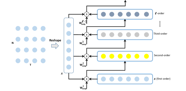
The overall framework of DeepCN is illustrated in Fig. 2. Given a multivariate time series input ${X}\in\mathbb{R}^{N\times T}$ where $N$ is the number of variables and $T$ is the look-back window size, first we conduct a reshape operation to transform the input ${X}\in\mathbb{R}^{N\times T}$ to a vector ${\bm{x}}\in\mathbb{R}^{NT\times 1}$. Next, $\bm{x}$ serves as input to the coupling mechanism which is designed to comprehensively explore the complicated intra- and inter-series relationships according to the analysis in Section 4. It applies explicit variable crossing of different time lags and outputs the corresponding couplings $\mathcal{C}^{2:\ell}=\{\mathcal{C}^{2},...,\mathcal{C}^{\ell}\}$ where $\mathcal{C}^{\ell}\in\mathbb{R}^{NT\times 1}$ is the $\ell$-order coupling and $\ell$ is the number of order (details see in Subsection 5.2). Then we stack $\mathcal{C}^{2:\ell}$ with ${x}$ and get the multi-order couplings among time series $\mathcal{C}=\{\mathcal{C}^{1},...,\mathcal{C}^{\ell}\}$.

After that, $\mathcal{C}$ is fed to a fully connected layer and outputs the dense representation $h\in\mathbb{R}^{\ell\times d}$ where $d$ is the dimension size. Since different variables exhibit different patterns, we initialize a variable embedding matrix $W_{var}\in\mathbb{R}^{N\times d}$ to embed the variable and perform a multiplication between $h$ and $W_{var}$ to represent variable relationships $\mathcal{X}\in\mathbb{R}^{N\times\ell\times d}$. Finally, we utilize a feed-forward network consisting of two fully connected layers and an activation function to predict the next $\tau$ timestamps $\hat{{X}}\in\mathbb{R}^{N\times\tau}$ by one forward step. The above content is explained in detail below.

5.2. Coupling Mechanism

A crucial element of our proposed model is the coupling mechanism, which plays a pivotal role in explicitly exploring diverse and hierarchical couplings to capture the complex multi-order intra- and inter-series relationships within time series. In Section 4, we have thoroughly analyzed the characteristics of relationships within time series data. In this subsection, we leverage these insights to design a coupling mechanism that effectively represents relationships based on those identified characteristics, such as multi-order couplings and the time lag effect. This mechanism is integral to our model’s ability to model and capture the intricate dependencies within the multivariate time series data.

According to Equation (5), the relationships within time series can be expressed through the couplings between different combinations of time lags of time series. Intuitively, the multi-order couplings can be modeled by cross feature (Wang et al., 2017). In light of the content introduced in Subsection 2.4, we understand that combinatorial features are essential in commercial models (Lian et al., 2018). The Cartesian Product model, as a state-of-the-art instance of a combinatorial-based model (Zhou et al., 2020), is an explicit model. Motivated by this, to explore the $\ell$-order couplings between $Z$ and ${X}_{1:N}^{t-T+1:t}$, we leverage the Cartesian product to illustrate how to calculate it. First, the Cartesian product $Cart_{\ell}$ can be defined as follows:

(6) $$\begin{split}Cart_{\ell}=\{(\underbrace{X_{i},X_{j},...,X_{l}}_{\ell})|X_{i,j,...,l}\in X_{1:N}^{t-T+1:t},\forall i,j,...,l=1,2,...,N\}\end{split}$$

where $N$ is the number of variables and $T$ is the length of timestamps. To illustrate this definition more intuitively, we use second-order couplings, five-time delay steps, and four variables as an example in Fig. 3. In the example, there are various combinations of cross variables and cross time, and several of them are marked with dotted lines in the figure.

Figure 3. Multi-order couplings diagram. In the figure, we take four variables, five time lags, and second-order as an example. From the figure, there are various combinations of cross-variable and cross-time, and several of them are marked with dotted lines. Moreover, the combinations include both intra-series (e.g., $\{X_{1}^{t-2}X_{1}^{t-3}\},\{X_{1}^{t-1}X_{1}^{t-3}\}$) and inter-series (e.g., $\{X_{1}^{t}X_{3}^{t}\},\{X_{2}^{t-2}X_{4}^{t-1}$}) information.

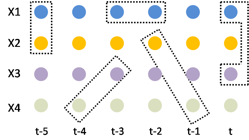
As evident from Equation (6), $Cart_{\ell}$ encompasses all possible combinations of $N$ variables from timestamps $t-T+1$ to timestamps $t$. These combinations include both intra-series correlations (e.g., the intra-series correlations for $X_{1}$ from timestamps $t-T+1$ to timestamps $t$, $X_{1}^{t-T+1}X_{1}^{t-T+2}...X_{1}^{t}$) and inter-series correlations (e.g., the inter-series correlations among $X_{1},X_{2},...,X_{N}$ at timestamps $t$, $X_{1}^{t}X_{2}^{t}...X_{N}^{t}$).

Inspired by the cross network (Wang et al., 2017) that has linear complexity, we achieve these combinations explicitly via efficiently learning all types of cross features. First, we reshape the input matrix $X\in\mathbb{R}^{N\times T}$ to a vector ${x}\in\mathbb{R}^{NT\times 1}$. Then we adopt the approach of feature interactions to model the relationships, and we can get the $\ell$-order couplings as follows:

(7) $$\begin{split}\mathcal{C}^{\ell}={x}{(\mathcal{C}^{\ell-1})}^{T}W_{coup}^{\ell-1}+b_{coup}^{\ell-1},\ell>1\\ \mathcal{C}^{1}={x},\ell=1\end{split}$$

where $W_{coup}^{\ell-1}\in\mathbb{R}^{NT\times 1},b_{coup}^{\ell-1}\in\mathbb{R}^{NT\times 1}$ are weight and bias parameters, respectively. Note that the first-order coupling, namely $\mathcal{C}^{1}$, is the input ${x}$ itself. The detailed calculation process is shown in Fig. 4 and the algorithm is described in Algorithm 1. According to Equation (7), we can find that it can fully explore all types of combinations of $X$. Different values of $\ell$ correspond to different order couplings. For example, when $\ell=2$, $\mathcal{C}^{\ell}$ corresponds to second-order couplings. Accordingly, we can express the hierarchical couplings $\mathcal{C}$ which are composed of various order couplings as follows:

(8) $$\mathcal{C}=(\mathcal{C}^{1},\mathcal{C}^{2},...,\mathcal{C}^{\ell})$$

where $\ell$ is the total number of orders.

Complexity Analysis. Let $\ell$ denote the total number of orders, $N$ denote the number of variables, and $T$ denote the look-back window size. Then the total number of parameters, namely $W_{coup}$ and $b_{coup}$ in Equation (7), is

(9) $$\ell\times N\times T\times 2.$$

From Equation (9), we can conclude that the complexity of the coupling mechanism is linearly proportional to the orders $\ell$, the number of variables $N$, and the input length $T$. In general, $T$ is much smaller than $N$.

Figure 4. Coupling-based model for relationships between variables. First, we transform the input matrix $X\in\mathbb{R}^{N\times T}$ to an input vector ${x}=\mathbb{R}^{NT\times 1}$ by a reshape operation where N is the number of variables and $T$ is the input length. Then we calculate the different order couplings respectively. $x$ is the first order.

Algorithm 1 Coupling Mechanism

0:  multivariate time series ${X}^{t}\in\mathbb{R}^{N\times T}$

0:  the multi-order couplings $\mathcal{C}\in\mathbb{R}^{\ell\times NT}$

1:  Given the multivariate time series input at timestamp t, $X^{t}\in\mathbb{R}^{N\times T}$

2:  Reshape $X$ into a vector ${x}\in\mathbb{R}^{NT\times 1}$

3:  Initialize the couplings $\mathcal{C}$

4:  $\mathcal{C}^{1}={x}$

5:  for $i=2,...,\ell$ do

6:     Initialize weight vector $W_{coup}^{i-1}\in\mathbb{R}^{NT\times 1}$

7:     Initialize bias vector $b_{coup}^{i-1}\in\mathbb{R}^{NT\times 1}$

8:     $\mathcal{C}^{i}={x}(\mathcal{C}^{i-1})^{T}W_{coup}^{i-1}$ + $b_{coup}^{i-1}$

9:  end for

10:  $\mathcal{C}=\{\mathcal{C}^{1},...,\mathcal{C}^{\ell}\}$

11:  return $\mathcal{C}$

5.3. Coupled Variable Representation Module

The resultant output $\mathcal{C}$ from the coupling mechanism captures a comprehensive representation of both intra- and inter-series dependencies among time series, including first-order coupling, second-order coupling, and beyond. However, given different variables may exhibit distinct patterns, we employ a coupled variable representation module to learn specific representations of the relationships between variables. The module helps to accommodate the diverse nature of MTS data and enables the model to better understand and represent the unique dependencies embodied in MTS.

To start, the output $\mathcal{C}\in\mathbb{R}^{\ell\times NT}$ from the coupling mechanism is inputted into a fully connected network, generating a dense representation $h\in\mathbb{R}^{\ell\times d}$, where $d$ represents the dimension size. Next, we initialize a variable embedding weight matrix $W_{var}\in\mathbb{R}^{d\times N}$ and perform multiplication with the dense representation $h$, resulting in an output $\mathcal{X}\in\mathbb{R}^{N\times\ell\times d}$. The calculation can be described as follows:

(10) $$\begin{split}h=\mathcal{C}W_{h}+b_{h},\\ \mathcal{X}=h\times W_{var}\end{split}$$

where $W_{h}\in\mathbb{R}^{NT\times d}$ and $b_{h}\in\mathbb{R}^{\ell\times d}$ is the weight matrix and bias matrix, respectively, $W_{var}\in\mathbb{R}^{d\times N}$ is the variable embedding weight matrix.

5.4. Inference Module

The inference module, which consists of a $ReLU$ activation function and two linear networks, is utilized to make predictions based on the output of the coupled variable representation $\mathcal{X}$. To prevent error accumulation, we generate all prediction values with a single forward step, which has proven to be more efficient and stable compared to step-by-step prediction (as demonstrated in Section 6). The formulation of the inference module is as follows:

(11) $$\hat{{X}}=\sigma(\mathcal{X}{W}_{1}+{b}_{1}){W}_{2}+{b}_{2}$$

where $\mathcal{X}\in\mathbb{R}^{N\times\ell\times d}$ is the output of coupled variable representation module, $\sigma$ is the activation function, ${W}_{1}\in\mathbb{R}^{(\ell*d)\times d_{h}},{W}_{2}\in\mathbb{R}^{d_{h}\times\tau}$ are the weights, and ${b}_{1}\in\mathbb{R}^{d_{h}}$, ${b}_{2}\in\mathbb{R}^{\tau}$ are the biases, and $d_{h}$ is the inner-layer dimension size. The final loss can be formulated as follows:

(12) $$\mathcal{L}(\hat{X},X;\Theta)=\sum_{t}\left\|\hat{X}^{t+1:t+\tau}-X^{t+1:t+\tau}\right\|_{2}^{2}$$

where $\tau$ is the prediction length, $\Theta$ is the learnable parameters, $\hat{X}$ is the prediction values and $X$ is the ground truth.

6. Experiments

In this section, we conduct a comprehensive evaluation of our proposed DeepCN model, assessing its prediction accuracy and computational efficiency. Additionally, we provide in-depth analyses of DeepCN, including a study of the coupling mechanism, an ablation study, a model analysis, and a visualization analysis. These evaluations aim to offer a thorough understanding of the capabilities and performance of our DeepCN model.

6.1. Datasets

We perform extensive experiments on seven real-world datasets, and a summary of these datasets is presented in Table 2. To ensure uniformity, all datasets are normalized using min-max normalization. Regarding data splitting, we divide all datasets, except for the COVID-19 dataset, into training, validation, and test sets, maintaining a chronological order with a ratio of 7:2:1. Given the relatively small sample size of the COVID-19 dataset, we have adjusted the data splitting ratio to 6:2:2.

Solar: This data set is about solar power collected by NREL (National Renewable Energy Laboratory). We use the usage of a state as the data set which contains 593 points. The data has been collected from 2006/01/01 to 2016/12/31 with the sampling interval of every 1 hour.

Wiki: The data set contains a number of daily views of different Wikipedia articles which have been collected from 2015/7/1 to 2016/12/31. It consists of approximately 145k time series and we choose 2k of them as our experimental data set due to limited computing resources.

Traffic: The data set contains a number of hourly traffic data of 963 San Francisco freeway car lanes which are collected from 2015/01/01 with the sampling interval of every 1 hour.

ECG: The data set is about Electrocardiogram(ECG) from the UCR time-series classification archive (Dau et al., 2018). It contains 140 nodes and each node has a length of 5000.

COVID-19: The dataset is about COVID-19 hospitalization in the U.S. state of California (CA) from 01/02/2020 to 31/12/2020 provided by the Johns Hopkins University with the sampling interval of every day.

Electricity: This dataset contains the electricity consumption of 370 clients and is collected since 2011/01/01. The data sampling interval is every 15 minutes.

METR-LA: This dataset contains traffic information collected from loop detectors in the highway of Los Angeles County from 01/03/2012 to 30/06/2012. It contains 207 sensors and the data sampling interval is every 5 minutes.

Table 2. Summary of Experimental Datasets

Datasets	Solar	Wiki	Traffic	ECG	COVID-19	Electricity	METR-LA
Samples	3650	803	10560	5000	335	140211	34272
Variables	592	5000	963	140	55	370	207
Granularity	1hour	1day	1hour	-	1day	15min	5min
Start time	01/01/2006	01/07/2015	01/01/2015	-	01/02/2020	01/01/2011	01/03/2012

6.2. Baselines

We compare our DeepCN with twenty-three representative and state-of-the-art (SOTA) models, including a classic model, DNN-based models, matrix factorization models, GNN-based models, Transformer-based models, and representation learning models.

Classic Model.

• VAR: VAR (Watson, 1993) is a classic linear autoregressive model. We use the Statsmodels library which is a Python package that provides statistical computations to realize the VAR.

DNN-based models.

• DA-RNN: DA-RNN (Qin et al., 2017) proposes a novel dual-stage attention-based recurrent neural network, consisting of an encoder with an input attention mechanism and a decoder with a temporal attention mechanism. We follow the recommended settings.

• LSTNet: LSTNet (Lai et al., 2018) uses a CNN to capture inter-variable relationships and an RNN to discover long-term patterns. In our experiment, we use the settings where the number of CNN hidden units is 100, the kernel size of the CNN layers is 4, the dropout is 0.2, the RNN hidden units is 100, the number of RNN hidden layers is 1, the learning rate is 0.001 and the optimizer is Adam.

• TCN: TCN (Bai et al., 2018) is a causal convolution model for regression prediction. We utilize the same configuration as the polyphonic music task exampled in the open source code where the dropout is 0.25, the kernel size is 5, the number of hidden units is 150, the number of levels is 4 and the optimizer is Adam.

• SFM: On the basis of the LSTM model, SFM (Zhang et al., 2017) introduces a series of different frequency components in the cell states. We use the default settings as the authors recommended where the learning rate is 0.01, the frequency dimension is 10, the hidden dimension is 10 and the optimizer is RMSProp.

• DLinear: DLinear (Zeng et al., 2023) proposes a set of embarrassingly simple one-layer linear models to learn temporal relationships between input and output sequences. We use it as our baseline and follow the recommended settings as experimental configurations.

• N-BEATS: N-BEATS (Oreshkin et al., 2019) utilizes stacked MLP layers together with doubly residual learning to process the input data to iteratively forecast the future. We follow the recommended settings as experimental configurations with 10 stacks, 4 layers, and 256 layer sizes.

• N-HiTS: N-HiTS (Challu et al., 2022) incorporates novel hierarchical interpolation and multi-rate data sampling techniques to improve forecast accuracy and reduce computational complexity. We use the recommended settings with 3 blocks, 9 layers, hidden size being 512, and learning rate being $0.001$.

Matrix factorization models.

• DeepGLO: DeepGLO (Sen et al., 2019) models the relationships among variables by matrix factorization and employs a temporal convolution neural network to introduce non-linear relationships. We use the default setting as our experimental settings for the Wiki, Electricity, and Traffic datasets. For the COVID-19 dataset, the vertical and horizontal batch size is set to 64, the rank of the global model is set to 64, the number of channels is set to [32, 32, 32, 1], and the period is set to 7.

GNN-based models.

• StemGNN: StemGNN (Cao et al., 2020) leverages GFT and DFT to capture dependencies among variables in the frequency domain. We use the default setting of StemGNN as our experiment setting where the optimizer is RMSProp, the learning rate is 0.0001, the stacked layers is 5, and the dropout rate is 0.5.

• MTGNN: MTGNN (Wu et al., 2020) proposes an effective method to exploit the inherent dependency relationships among multiple time series. Because the experimental datasets have no static features, we set the parameter load_static_feature to false. We construct the graph by the adaptive adjacency matrix and add the graph convolution layer. Regarding other parameters, we adopt the default settings.

• GraphWaveNet: GraphWaveNet (Wu et al., 2019) introduces an adaptive dependency matrix learning to capture the hidden spatial dependency. Since our datasets have no prior defined graph structures, we use only adaptive adjacent matrix. We add a graph convolutional layer and randomly initialize the adjacent matrix. We adopt the default setting as our experimental settings where the learning rate is 0.001, the dropout is 0.3, the number of epochs is 50, and the optimizer is Adam.

• AGCRN: AGCRN (Bai et al., 2020) proposes a data-adaptive graph generation module for discovering spatial correlations from data. We use the default settings as our experimental settings where the embedding dimension is 10, the learning rate is 0.003, and the optimizer is Adam.

• TAMP-S2GCNets: TAMP-S2GCNets (Chen et al., 2022) explores the utility of MP to enhance knowledge representation mechanisms within the time-aware DL paradigm. TAMP-S2GCNets require a pre-defined graph topology and we use the California State topology provided by the source code as input. We adopt the recommended settings as the experimental configuration for COVID-19.

• DCRNN: DCRNN (Li et al., 2018) uses bidirectional graph random walk to model spatial dependency and recurrent neural network to capture the temporal dynamics. We use the recommended configuration as our experimental settings with a batch size of 64, the learning rate being $0.01$, the input dimension being 2, and the optimizer of Adam. DCRNN requires a pre-defined graph structure and we use the adjacency matrix as the pre-defined structure provided by the METR-LA dataset.

• STGCN: STGCN (Yu et al., 2018) integrates graph convolution and gated temporal convolution through spatial-temporal convolutional blocks. We follow the recommended settings as our experimental configuration where the batch size is 50, the learning rate is $0.001$ and the optimizer is Adam. STGCN requires a pre-defined graph structure and we leverage the adjacency matrix as the pre-defined structure provided by the METR-LA dataset.

Transformer-based models.

• Informer: Informer (Zhou et al., 2021) leverages an efficient self-attention mechanism to encode the dependencies among variables. We use the default settings as our experimental settings where the dropout is 0.05, the number of encoder layers is 2, the number of decoder layers is 1, the learning rate is 0.0001, and the optimizer is Adam.

• Reformer: Reformer (Kitaev et al., 2020) combines the modeling capacity of a Transformer with an architecture that can be executed efficiently on long sequences and with small memory use. We follow the recommended settings.

• Autoformer: Autoformer (Wu et al., 2021) proposes a decomposition architecture by embedding the series decomposition block as an inner operator, which can progressively aggregate the long-term trend part from intermediate prediction. We follow the recommended settings with 2 encoder layers and 1 decoder layer.

• PatchTST: PatchTST (Nie et al., 2023) proposes an effective design of Transformer-based models for time series forecasting tasks by introducing two key components: patching and channel-independent structure. We use it as our forecasting baseline and adhere to the recommended settings as the experimental configuration.

Representation learning-based models.

• TS2Vec: TS2Vec (Yue et al., 2022) is a universal framework for learning representations of time series in an arbitrary semantic level. Following the recommended settings, we set the representation dimension to 320, the hidden dimension of the encoder to 64, the number of hidden residual blocks to 10, and the learning rate to 0.001.

• InfoTS: InfoTS (Luo et al., 2023) proposes a new contrastive learning approach with information-aware augmentations that adaptively selects optimal augmentations for time series representation learning. We set the representation dimension to 320, the hidden dimension to 60, and the meta learning rate to 0.01.

• CoST: CoST (Woo et al., 2022) separates the representation learning and downstream forecasting task and proposes a contrastive learning framework that learns disentangled season-trend representations for time series forecasting tasks. We set the representation dimension to 320, the learning rate to 0.001, and the batch size to 32.

6.3. Experimental Setup

We perform our experiments on a single NVIDIA RTX 3080 10G GPU. Our code is implemented by Python 3.6 with PyTorch 1.9. Our model is optimized with RMSprop optimizer and the learning rate is $1e^{-5}$. Across all datasets, batch size is set to 32. The number of epochs is 50. For the Traffic, Electricity, METR-LA, and COVID-19 datasets, the dimension size $d$ is set to 512. For the Wiki, Solar, and ECG datasets, the dimension size $d$ is set to 1024. For the COVID-19, ECG, and Electricity datasets, the number of orders $\ell$ is set to 2. For the Wiki and Traffic datasets, $\ell$ is set to 4. For the Solar and METR-LA datasets, $\ell$ is set to 3. In the inference module, the hidden size is 1024 and the activation function is $ReLU$.

We use MAE and RMSE as metrics. Specifically, given the groudtruth $X^{t+1:t+\tau}_{1:N}\in\mathbb{R}^{N\times\tau}$ and the predictions $\hat{X}^{t+1:t+\tau}_{1:N}\in\mathbb{R}^{N\times\tau}$ for future $\tau$ steps at timestamp $t$, the metrics are defined as follows:

(13) $$MAE=\frac{1}{\tau N}\sum_{i=1}^{N}\sum_{j=1}^{\tau}\left|X_{i}^{j}-\hat{X}_{i}^{j}\right|$$

(14) $$RMSE=\sqrt{\frac{1}{\tau N}\sum_{i=1}^{N}\sum_{j=1}^{\tau}\left(X_{i}^{j}-\hat{X}_{i}^{j}\right)^{2}}.$$

Table 3. Single step forecasting error results (MAE and RMSE) of DeepCN and other baseline models on five datasets with the prediction length being 12 and the input length being 12.

Dataset	Solar		Wiki		Traffic		ECG		COVID-19		Electricity
Metrics	MAE	RMSE	MAE	RMSE	MAE	RMSE	MAE	RMSE	MAE	RMSE	MAE	RMSE
VAR	0.184	0.234	0.057	0.094	0.535	1.133	0.120	0.170	0.226	0.326	0.101	0.163
SFM	0.161	0.283	0.081	0.156	0.029	0.044	0.095	0.135	0.205	0.308	0.086	0.129
LSTNet	0.148	0.200	0.054	0.090	0.026	0.057	0.079	0.115	0.248	0.305	0.075	0.138
TCN	0.176	0.222	0.094	0.142	0.052	0.067	0.078	0.107	0.317	0.354	0.057	0.083
DA-RNN	0.156	0.214	0.060	0.104	0.036	0.055	0.074	0.108	0.212	0.278	0.068	0.114
DeepGLO	0.178	0.400	0.110	0.113	0.025	0.037	0.110	0.163	0.191	0.253	0.090	0.131
Reformer	0.234	0.292	0.047	0.083	0.029	0.042	0.062	0.090	0.182	0.249	0.078	0.129
Informer	0.151	0.199	0.051	0.086	0.020	0.033	0.056	0.085	0.200	0.259	0.070	0.119
Autoformer	0.150	0.193	0.069	0.103	0.029	0.043	0.055	0.081	0.189	0.241	0.056	0.083
FEDformer	0.139	0.182	0.068	0.098	0.025	0.038	0.055	0.080	0.190	0.259	0.055	0.081
GraphWaveNet	0.183	0.238	0.061	0.105	0.013	0.034	0.093	0.142	0.201	0.255	0.094	0.140
StemGNN	0.176	0.222	0.190	0.255	0.080	0.135	0.100	0.130	0.421	0.508	0.070	0.101
MTGNN	0.151	0.207	0.101	0.140	0.013	0.030	0.096	0.145	0.394	0.488	0.077	0.113
AGCRN	0.143	0.214	0.044	0.079	0.084	0.166	0.055	0.080	0.254	0.309	0.074	0.116
N-BEATS	0.139	0.182	0.047	0.087	0.016	0.031	0.056	0.088	0.192	0.292	0.057	0.085
N-HITS	0.129	0.174	0.046	0.083	0.018	0.035	0.055	0.086	0.185	0.283	0.060	0.089
DLinear	0.257	0.313	0.182	0.219	0.046	0.064	0.133	0.176	0.306	0.382	0.058	0.092
PatchTST	0.140	0.234	0.050	0.094	0.016	0.037	0.054	0.080	0.230	0.289	0.058	0.094
TS2Vec	0.141	0.184	0.045	0.080	0.021	0.034	0.053	0.078	0.376	0.439	0.105	0.156
InfoTS	0.142	0.186	0.052	0.094	0.027	0.049	0.052	0.077	0.330	0.412	0.068	0.104
DeepCN(ours)	0.132	0.172	0.042	0.078	0.011	0.022	0.051	0.076	0.170	0.232	0.053	0.078
Improvement	5.0%	5.5%	4.5%	1.3%	15.4%	26.7%	1.9%	1.3%	6.6%	3.7%	3.6%	3.7%

6.4. Results

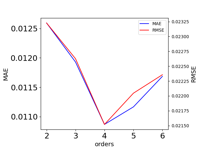
Single-step forecasting. We compare our model DeepCN against the other baseline models on seven real-world datasets with the input length being 12 and the prediction length being 12. The primary results are summarized in Table 3. As indicated in the table, DeepCN consistently demonstrates strong performance across all datasets. On the Solar dataset, DeepCN improves 5.0$\%$ on MAE and 5.5$\%$ on RMSE. On the Wiki dataset, it improves 4.5$\%$ on MAE and 1.3$\%$ on RMSE. On the ECG dataset, it improves 1.9$\%$ on MAE and 1.3$\%$ on RMSE. On the COVID-19 dataset, it improves 6.6$\%$ on MAE and 3.7$\%$ on RMSE. On the Electricity dataset, it improves 3.6$\%$ on MAE and 3.7$\%$ on RMSE. Especially, on the Traffic dataset, DeepCN improves 15.4$\%$ on MAE and 26.7$\%$ on RMSE compared with the best baseline. The reason why DeepCN performs exceptionally well on the Traffic dataset is because of the strong coupling in the traffic data. For example, adjacent nodes affect each other, and adjacent areas also affect each other. If a road is jammed, it inevitably affects other roads. We conduct more experiments on the couplings of the Traffic dataset, and the result is shown in Fig. 9(a). From the figure, we conclude there are multi-order couplings in the Traffic dataset. This also sheds light on the superior accuracy of DeepCN, as it incorporates the consideration of multi-order couplings.

Among these baseline models, transformer-based models and GNN-based models have achieved more competitive performance than other DNN-based models. As shown in Fig. 1, DNN-based models can not attend to the time lag effect directly and ignore the inter-series relationships. The two inherent defects affect their ability to capture the dependencies among time series. Moreover, GNN-based models perform well on Solar, Wiki, Traffic, and ECG datasets while transformer-based models achieve good results only on COVID-19 and ECG datasets. This is because compared with transformer-based models, GNN-based models consider inter-series relationships. The results also indicate the significance of inter-series relationships in MTS forecasting, especially in tight coupling scenarios like traffic forecasting.

Table 4. Multi-step forecasting error results (MAE and RMSE) on ECG dataset. We compare DeepCN with the other six baseline models on the ECG dataset when the prediction length is 3, 6, 9, and 12, respectively.

Horizon	3		6		9		12
Metrics	MAE	RMSE	MAE	RMSE	MAE	RMSE	MAE	RMSE
LSTNet	0.085	0.178	0.128	0.202	0.128	0.202	0.128	0.203
DeepGLO	0.083	0.142	0.093	0.161	0.107	0.157	0.110	0.163
Informer	0.055	0.083	0.055	0.084	0.057	0.086	0.056	0.085
GraphWaveNet	0.090	0.139	0.092	0.141	0.095	0.145	0.097	0.149
StemGNN	0.090	0.130	0.100	0.130	0.090	0.129	0.100	0.130
MTGNN	0.092	0.140	0.094	0.140	0.095	0.144	0.096	0.145
DeepCN(ours)	0.050	0.076	0.050	0.076	0.051	0.076	0.051	0.076
Improvement	9.1%	8.4%	9.1%	9.5%	10.5%	11.6%	8.9%	10.6%

Table 5. Multi-step forecasting error results (MAE and RMSE) on Traffic dataset. We compare DeepCN with the other seven baseline models on the Traffic dataset when the prediction length is 3, 6, 9, and 12, respectively.

Horizon	3		6		9		12
Metrics	MAE	RMSE	MAE	RMSE	MAE	RMSE	MAE	RMSE
VAR	0.047	0.076	0.095	0.150	0.182	0.319	0.535	1.133
LSTNet	0.016	0.038	0.019	0.045	0.023	0.051	0.026	0.057
DeepGLO	0.020	0.036	0.022	0.036	0.024	0.038	0.025	0.037
Informer	0.019	0.031	0.020	0.032	0.020	0.032	0.020	0.033
GraphWaveNet	0.011	0.027	0.013	0.031	0.013	0.030	0.013	0.034
StemGNN	0.050	0.093	0.070	0.121	0.090	0.144	0.080	0.135
MTGNN	0.011	0.026	0.012	0.027	0.012	0.028	0.013	0.030
DeepCN(ours)	0.009	0.020	0.010	0.021	0.011	0.021	0.011	0.022
Improvement	18.2%	23.1%	16.7%	22.2%	8.3%	25.0%	15.4%	26.7%

Table 6. Multi-step forecasting error results (MAE and RMSE) on Wiki dataset. We compare DeepCN with other five baseline models on Traffic dataset when prediction length is 3, 6, 9, and 12, respectively.

Length	3		6		9		12
Metrics	MAE	RMSE	MAE	RMSE	MAE	RMSE	MAE	RMSE
GraphWaveNet	0.061	0.105	0.061	0.105	0.061	0.105	0.061	0.104
StemGNN	0.157	0.236	0.159	0.233	0.232	0.311	0.220	0.306
AGCRN	0.043	0.077	0.044	0.078	0.045	0.079	0.044	0.079
MTGNN	0.102	0.141	0.091	0.133	0.074	0.120	0.101	0.140
Informer	0.053	0.089	0.054	0.090	0.059	0.095	0.059	0.095
DeepCN(ours)	0.041	0.076	0.042	0.076	0.042	0.077	0.042	0.078
Improvement	4.7%	1.3%	4.5%	2.6%	6.7%	2.5%	4.5%	1.3%

Table 7. Multi-step forecasting error results (MAE and RMSE) on METR-LA dataset. We compare DeepCN with other eight baseline models on METR-LA dataset when prediction length is 3, 6, 9, and 12, respectively.

Horizon	3		6		9		12
Metrics	MAE	RMSE	MAE	RMSE	MAE	RMSE	MAE	RMSE
DCRNN	0.160	0.204	0.191	0.243	0.216	0.269	0.241	0.291
STGCN	0.058	0.133	0.080	0.177	0.102	0.209	0.128	0.238
GraphWaveNet	0.180	0.366	0.184	0.375	0.196	0.382	0.202	0.386
MTGNN	0.135	0.294	0.144	0.307	0.149	0.328	0.153	0.316
StemGNN	0.052	0.115	0.069	0.141	0.080	0.162	0.093	0.175
AGCRN	0.062	0.131	0.086	0.165	0.099	0.188	0.109	0.204
Informer	0.076	0.141	0.088	0.163	0.096	0.178	0.100	0.190
CoST	0.064	0.118	0.077	0.141	0.088	0.159	0.097	0.171
DeepCN(ours)	0.051	0.114	0.068	0.140	0.078	0.159	0.090	0.168
Improvement	1.9%	0.9%	1.4%	0.7%	2.5%	-	3.2%	1.8%

Multi-step forecasting. In order to further evaluate the accuracy of DeepCN under different prediction lengths, we conduct more experiments on multi-step forecasting, including 3, 6, 9, and 12 steps. We perform experiments on the ECG, Traffic, Wiki, and METR-LA datasets, respectively. For the ECG dataset, the input length of all models is set to 12. The coupling number $\ell$ of DeepCN is set to 2. As you can see from the results in Table 4, DeepCN achieves good performance in multi-step forecasting tasks as it improves an average of 9.4$\%$ on MAE and 10.0$\%$ on RMSE. Among the baselines, Informer performs better than others since it can model the intra-series dependencies directly. For the Traffic dataset, the input length of all models is also set to 12. The coupling number $\ell$ of DeepCN is set to 5. The results are shown in Table 5 and we can find that DeepCN improves an average of 14.7$\%$ on MAE and 24.3$\%$ on RMSE. Among the baselines, MTGNN shows good performance because it has good capability to capture the inter-series dependencies. For the Wiki dataset, we choose GNN-based models and Transformer-based model Informer as the baseline models, the input length is set to 12 and the number of orders $\ell$ is set to 4. The results in Table 6 demonstrate that our proposed model improves an average of 5.1$\%$ on MAE and 1.9$\%$ on RMSE. Among the baselines, AGCRN achieves competitive results since it constructs the graph structure (i.e., the inter-series dependencies) adaptively from time series data. For the METR-LA dataset, we compare DeepCN with the GNN-based, Transformer-based, and representation learning based models as our baselines, and the results are shown in Table 7. The table showcases that on average we improve $2.3\%$ on MAE and $1.1\%$ on RMSE. Among these models, StemGNN achieves competitive performance because it explicitly model both intra- and inter-series dependencies. However, it is limited to simultaneously capturing intra-/inter-series dependencies. CoST learns disentangled seasonal-trend representations for time series forecasting via contrastive learning and obtains competitive results. But, our model still outperforms CoST. Because, compared with CoST, our model not only can learn the dynamic intra-series representations, but also capture the discriminative inter-series representations.

Moreover, Fig. 5 and Fig. 6 exhibit the changing curve of the accuracy under different steps on the ECG dataset and Traffic dataset, respectively. From Fig. 5, we can find that as the steps increase, the accuracy rate of a classic model (VAR) decreases. It also shows that the accuracy of Informer is closer to ours, but LSTNet’s performance is not quite ideal on the ECG dataset. Fig. 6 shows that the accuracy of GNN-based models is closer to ours, whereas StemGNN presents poor accuracy on the Traffic dataset. In addition, from Fig. 5 and Fig. 6, we can observe that the accuracy of our proposed model DeepCN is stable when prediction length increases because DeepCN utilizes one forward step to make a prediction which can avoid error accumulations. Informer also makes predictions by one forward step and its accuracy shows stable while StemGNN adopting a rolling strategy has fluctuations in performance.

(a) Analysis on MAE

(b) Analysis on RMSE

Figure 5. Multi-step forecasting error result analysis (MAE and RMSE) on the ECG dataset. We compare the changing curve of DeepCN with the other five baseline models on the ECG dataset under different prediction lengths (3, 6, 9, 12), respectively.

(a) Analysis on MAE

(b) Analysis on RMSE

Figure 6. Multi-step forecasting error result analysis (MAE and RMSE) on the Traffic dataset. We compare the changing curve of our model with the other four baseline models on the Traffic dataset under different prediction lengths (3, 6, 9, 12), respectively. We delete the VAR model because its value is too large to affect the display.

Figure 7. The predicts (steps=12) of DeepCN and Informer on ECG dataset. The three different color curves stand for slices of the ground truth, Informer, and DeepCN, respectively. Four nodes were randomly selected from 140 in the dataset as observation variables to compare the ground truth with the prediction values of Informer and DeepCN. The above four subgraphs correspond to a node, respectively.

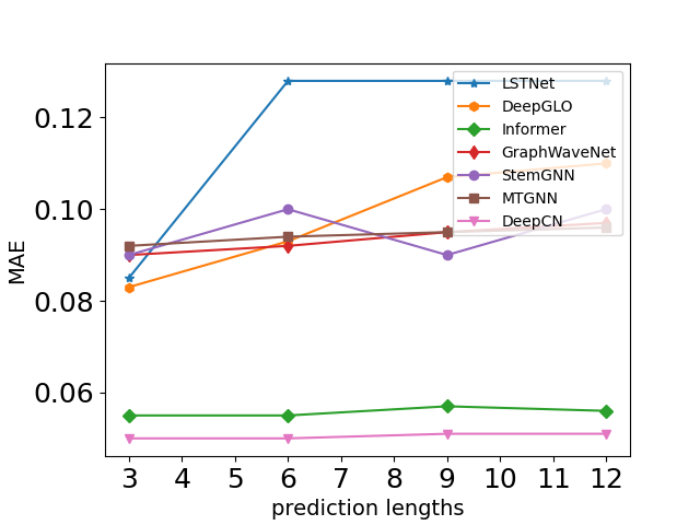
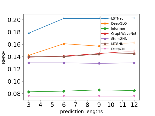
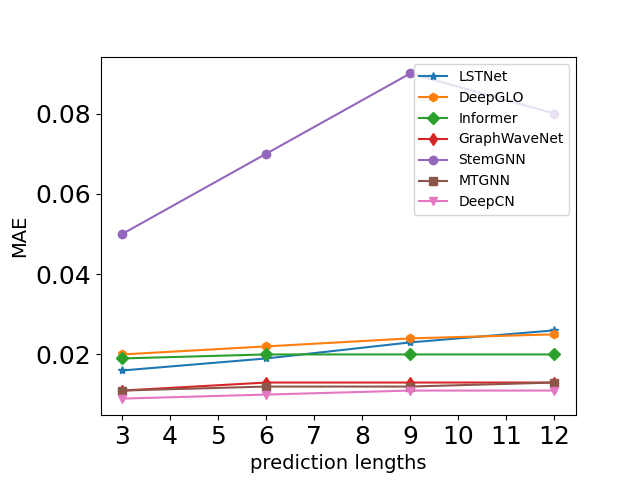
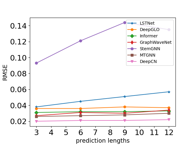
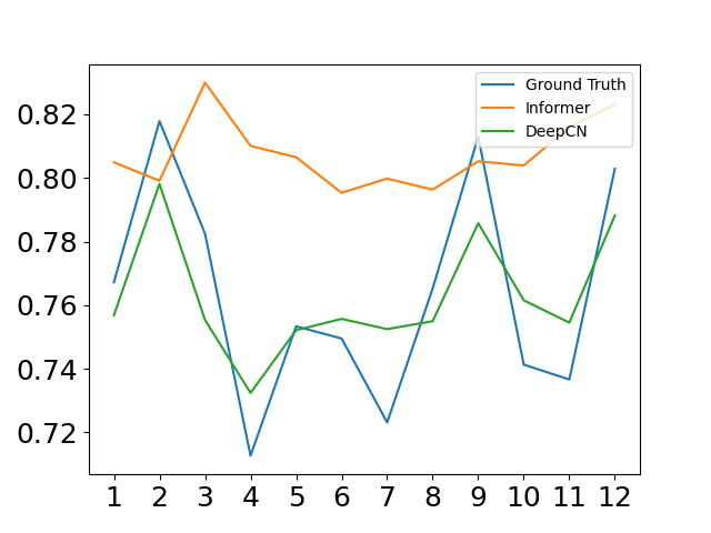
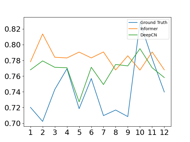
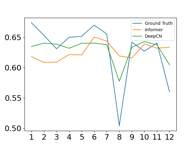
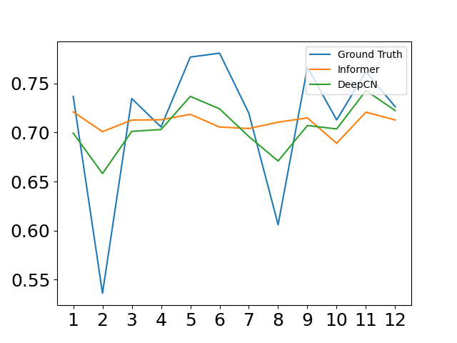
Fig. 7 shows the comparison of our proposed model and Informer between the predicted values and ground truth when the prediction length is 12. We choose Informer as the comparative baseline because it performs better compared with other models (as shown in Table 4). We randomly select four variables from the ECG dataset. Each subgraph corresponds to one variable. The x-coordinate represents the prediction time step and the y-coordinate represents the value. As shown in Fig. 7, the prediction performance of DeepCN is better than that of Informer and it is able to fit the curve of ground truth except for some sudden changes.

6.5. Analysis

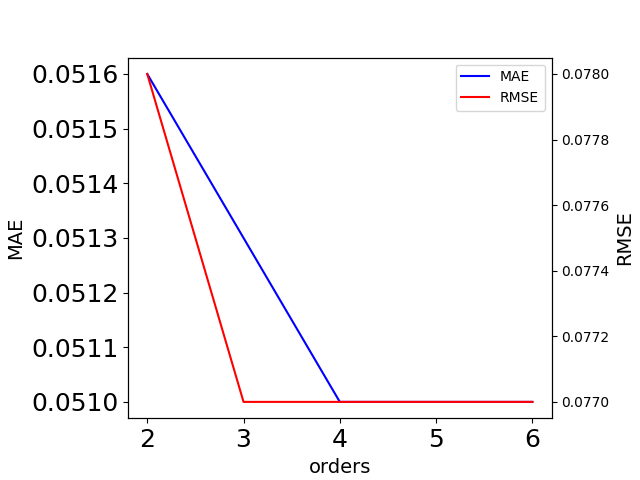
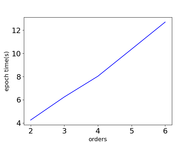
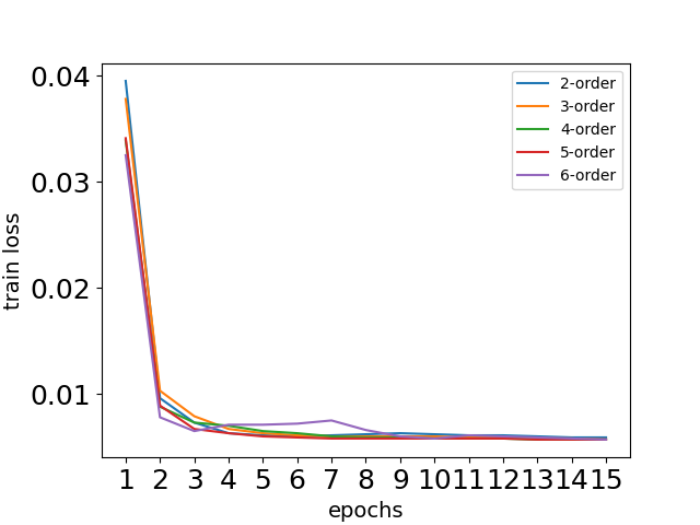
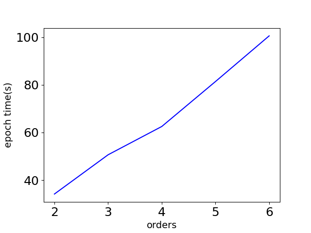
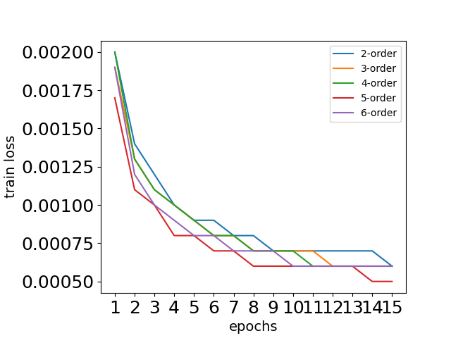
Study of the Coupling Mechanism. This part mainly addresses how the coupling mechanism affects the accuracy and efficiency of our proposed model. We conduct experiments by imposing a different number of coupling orders $\ell$ (e.g., second-order coupling, third-order coupling, fourth-order coupling, and so on) on the Traffic and ECG datasets, respectively. We separately analyze the relationship between training time and the number of coupling orders, and the relationship between error results (MAE and RMSE) and the number of coupling orders. The result on the ECG dataset is shown in Fig. 8 and the result on the Traffic data is shown in Fig. 9. From Fig. 8, we can see that: 1) As the number of orders $\ell$ increases, the training time becomes longer, but it has little effect on the convergence speed of training. 2) When the order $\ell$ is greater than 2, the accuracy is almost unchanged because the data on the ECG dataset has weak correlations among time series. Namely, the data on the ECG dataset does not exhibit high-order coupling characteristics. From Fig. 9, we can find that: 1) With the number of orders $\ell$ increasing, the training time becomes longer and the convergence rate of training does not change much. 2) The accuracy rate increases first which shows that higher-order couplings exist on the Traffic dataset. Then with $\ell$ increasing, the performance worsens since higher order leads to overfitting. From Fig. 8(a) and Fig. 9(a), we can conclude that for the strong inter-series correlation time series dataset (e.g., Traffic dataset), it is necessary to model the high-order couplings, while for the weak inter-series correlation dataset (e.g., ECG dataset), modeling for the high-order couplings does not bring improvements in effectiveness. This also explains that sequential models achieve generally better results than GNN-based models on the ECG dataset, while on the Traffic dataset, GNN-based models perform better than other models.

(a) accuracy analysis

(b) efficiency analysis

(c) train loss analysis

Figure 8. Study of coupling mechanism on ECG dataset. We analyze the accuracy, efficiency, and training loss of our model on the ECG dataset under different orders, respectively. (a) The error result (MAE and RMSE) under different orders. (b) The average training time under different orders. (c) The training loss in different epochs under different orders.

(a) accuracy analysis

(b) efficiency analysis

(c) train loss analysis

Figure 9. Study of coupling mechanism on the Traffic dataset. We analyze the accuracy, efficiency, and training loss of our model on the Traffic dataset under different orders, respectively. (a) The error result (MAE and RMSE) under different orders. (b) The average training time under different orders. (c) The training loss in different epochs under different orders.

Ablation Study. To further analyze the different orders of couplings, we conduct more experiments on the Traffic dataset and ECG dataset to evaluate the effectiveness of different orders. We set the input length and prediction length to 12, and the number of orders $\ell$ is set to 4. Other experimental settings are the same as introduced in Section 6.3. We evaluate the effectiveness of each order of coupling by masking the corresponding order. The results are shown in Table 8. In the table, w/o coupling means that the model is without the coupling mechanism. Namely, the model is only composed of the first-order coupling and the fully-connected network. w/o 1st represents the coupling mechanism without the first-order coupling and we mask the first-order coupling from the relationships $\mathcal{C}$. In a similar fashion, w/o 2st, w/o 3st, and w/o 4st represents the coupling mechanism without the second-order, third order and fourth-order couplings, respectively. From the table, we can find that: 1) For the Traffic dataset, each order of coupling is indispensable. 2) For the ECG dataset, compared with other orders of couplings, the first-order coupling is more important. It shows that the high-order couplings should be considered in the strong correlation data while the low-order coupling is enough for the relationship modeling in the weak correlation data.

Table 8. Error results (MAE and RMSE) under different orders of couplings

Dataset	Metrics	DeepCN	w/o coupling	w/o 1st	w/o 2st	w/o 3st	w/o 4st
Traffic	MAE	0.011	0.013	0.012	0.012	0.012	0.012
	RMSE	0.022	0.024	0.024	0.023	0.023	0.022
ECG	MAE	0.050	0.051	0.055	0.051	0.051	0.051
	RMSE	0.076	0.077	0.081	0.077	0.077	0.077

Efficiency Analysis. To evaluate the efficiency of DeepCN, we compare the training time and parameter counts of our proposed model with GNN-based models (StemGNN, AGCRN, and MTGNN) and Transformer-based models (Autoformer and Informer) on the Wiki and Traffic datasets, respectively. We use the same input length ($T=12$) and prediction length $(\tau=12)$ for the analysis in the five methods and the results are shown in Table 9. From the table, we can find that: 1) the Transformer-based models require less training time than GNN-based models and our model since they only model the intra-series dependencies while GNN-based models and our model consider both intra- and inter-series dependencies. 2) Compared with the GNN-based models, our proposed model performs more efficiently because the complexity of our model is $\mathcal{O}(N\times T)$ while the AGCRN and MTGNN are $\mathcal{O}(N^{2})$ and StemGNN is $\mathcal{O}(N^{3})$. 3) Transformer-based models consume more parameters than GNN-based models since the self-attention mechanism needs high memory usage. 4) The parameter count of our model is larger than GNN-based models because our model encodes not only timestamp-wise and variable-wise interactions but also multi-order couplings. Moreover, our model simultaneously models the intra- and inter-series dependencies while GNN-based models separately model them.

Table 9. Results of efficiency analysis on Wiki dataset (variables=1000, samples=803) and Traffic dataset (variables=962, samples=10560).

	Training time (s/epoch)
	DeepCN	StemGNN	AGCRN	MTGNN	Autoformer	Informer
Wiki	9.61	92.59	22.48	27.76	2.39	2.64
Traffic	62.52	201.69	166.61	169.34	14.48	12.99
	Parameters
	DeepCN	StemGNN	AGCRN	MTGNN	Autoformer	Informer
Wiki	7.91M	4.10M	0.76M	1.53M	15.6M	14.9M
Traffic	8.74M	3.88M	0.75M	1.48M	15.4M	14.8M

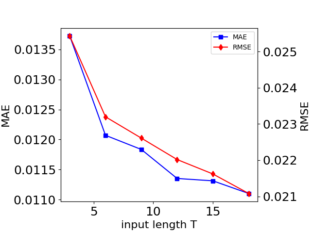
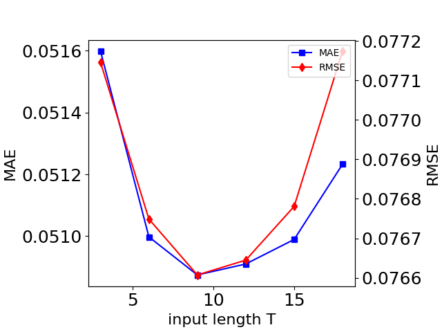
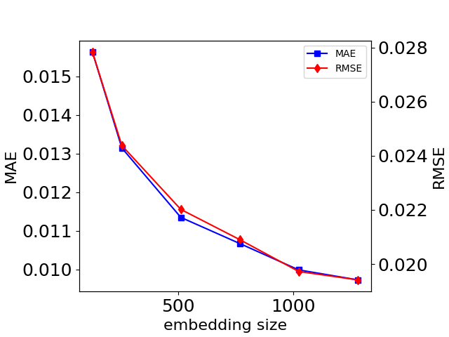
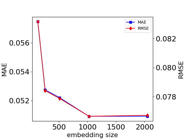
Parameter Sensitivity. We perform parameter sensitivity tests of input length $T$ and embedding size $d$ on the Traffic and ECG datasets. All parameters of our model under study are held constant except the input length and the embedding size. (1) Input length. The input length reflects the time lag effects and affects the final accuracy. We turn over it with the value $\{3,6,9,12,15,18\}$ for the Traffic and ECG datasets, and the result is shown in Fig. 10. Fig. 10(a) shows that with the input length increasing, the accuracy becomes better since the long input length can bring more information and this also demonstrates the relationships between variables have time lag effects which are introduced in Section 4. Fig. 10(b) shows that with the input length increasing, the performance first improves and then decreases due to data redundancy or overfitting. (2) Embedding size. The embedding size affects the representation ability and we choose the embedding size over the set $\{128,256,512,768,1024,1280\}$ for the Traffic dataset and $\{128,256,512,1024,2048\}$ for ECG dataset. We choose different value sets for the two datasets because of the memory limit. Fig. 11(a) demonstrates that the performance becomes better with the increase of embedding size while Fig. 11(b) shows that the performance first improves and then keeps almost unchanged. Unlike the data on the ECG dataset, the data on the Traffic dataset exhibits strong couplings between the data. Then compared with the ECG dataset, the data on the Traffic dataset has stronger time lag effects (comparing Fig. 10(a) with Fig. 10(b)), and needs bigger embedding size to represent the complicated relationships (comparing Fig. 11(a) with Fig. 11(b)).

(a) Traffic dataset

(b) ECG dataset

Figure 10. Parameter sensitivity analysis about input length. We compare error results (MAE and RMSE) under different input lengths on the Traffic and ECG datasets, respectively.

(a) Traffic dataset

(b) ECG dataset

Figure 11. Parameter sensitivity analysis about the embedding size. We compare error results (MAE and RMSE) under different embedding sizes on the Traffic and ECG datasets, respectively.

6.6. Visualization

To gain a better understanding of the coupling mechanism for modeling intra- and inter-series relationships among time series data, we further conduct experiments on the Wiki dataset to visualize the different order couplings.

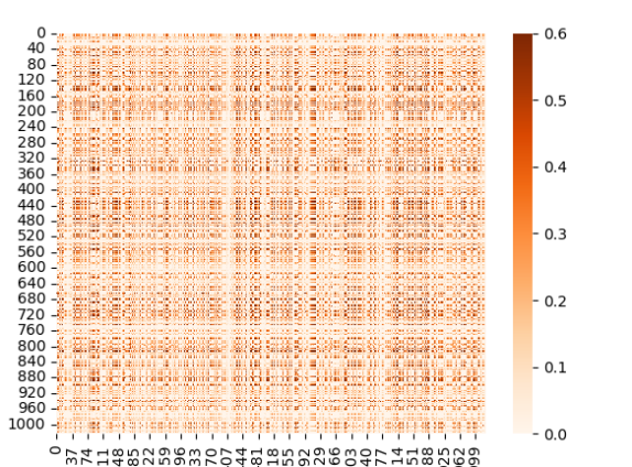
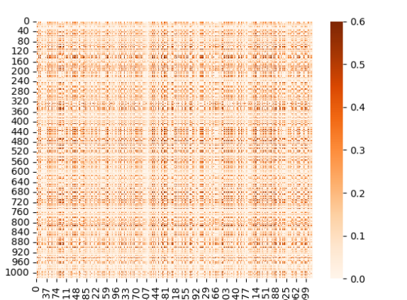
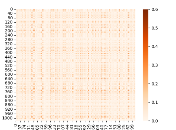
Visualization about heatmap of multi-order couplings In order to showcase the different impacts of each order of couplings in modeling the intra- and inter-series relationships, we generate the corresponding visual heatmap to represent them. Specifically, given the dense representations of couplings denoted as $\mathcal{X}\in\mathbb{R}^{\ell\times d}$, for each order $\ell$, we compute the weight matrix as follows: $W_{vis}^{(\ell)}=\mathcal{X}^{(\ell)}\times\{\mathcal{X}^{(\ell)}\}^{T}$. Subsequently, we visualize $W_{vis}^{(\ell)}\in\mathbb{R}^{d\times d}$ via a heatmap. In our experiments, we choose four order couplings (i.e., $\ell=4$), and the results are presented in Fig. 12(a). The figure demonstrates that: (1) All four order couplings are indispensable. (2) Among the four-order couplings, the second-order and third-order couplings hold greater significance in capturing both intra- and inter-series relationships. This also explains that although the SOTA GNN- and Transformer-based models are primarily based on second-order or third-order interactions while ignoring first-order and fourth-order couplings, they have still achieved competitive results in the realm of MTS forecasting.

(a) Heatmap visualization of multi-order couplings

(b) t-SNE visualization of multi-order couplings

Figure 12. (a) Visualizations of multi-order couplings learned from the Wiki dataset. (b) Visualizations about t-SNE of multi-order couplings learned from the Wiki dataset. Different subfigures/colors correspond to different order couplings: specifically first-order (upper left, blue), second-order(upper right, black), third-order (bottom left, red), and fourth-order (bottom right, grey).

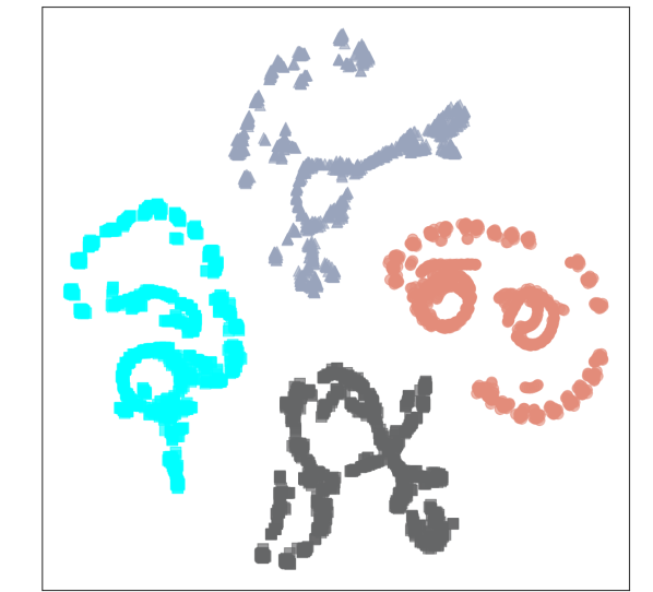
Visualization about t-SNE of multi-order couplings To investigate the relation between different order couplings, we create visualizations using t-SNE for these couplings. Concretely, for the dense representations of couplings represented as $\mathcal{X}\in\mathbb{R}^{\ell\times d}$, we generate t-SNE visualizations for each order of couplings, denoted as $\mathcal{X}^{(\ell)}\in\mathbb{R}^{d}$, individually. In our experiment, the order $\ell$ is 4, and the results are depicted in Fig. 12(b). The figure illustrates that the couplings of different orders are distinct and separate from each other.

Based on the insights drawn from Figs. 12(a) and 12(b), we can conclude that the coupling mechanism comprehensively explores the different order couplings that are disentangled, and it expressively learns representations of both intra- and inter-series relationships.

7. Conclusion

In this paper, to address the relationship modeling issues for MTS forecasting, we propose a novel model DeepCN for multivariate time series forecasting, including single-step forward prediction and multi-step forward prediction. Compared with the previous work, in this work, we build our model based on the couplings which can bring more comprehensive information to enhance representations of relationships among time series. Specifically, we first revisit the relationships among time series from the perspective of mutual information. Then based on the analysis, we design a coupling mechanism to learn the hierarchical and diverse couplings to represent the relationships that can exploit the intra- and inter-series relationships simultaneously. The coupling mechanism can model multi-order couplings and account for the time lag effect explicitly. After that, since different variables exhibit different patterns, we leverage a coupled variable representation module to learn the variable relationship representation. Finally, we make predictions by one forward step which can avoid error accumulation. The one-forward-step method makes our model more efficient and stable in the multi-step forward prediction. We conduct extensive experiments on seven real-world datasets and compare our model with other state-of-the-art baselines. The experimental results show that our model achieves superior performance. Furthermore, more analysis of our model demonstrates that different order couplings impose different effects on different datasets which gives us enlightenment for handling different types of MTS data. Compared with the state-of-the-art GNN-based models, DeepCN has relatively higher model complexity in terms of parameter volumes. In the future, we plan to move our work forward to reduce the parameter counts and the time complexity.