Physics-constrained polynomial chaos expansion for scientific machine learning and uncertainty quantification

Abstract

We present a novel physics-constrained polynomial chaos expansion as a surrogate modeling method capable of performing both scientific machine learning ( SciML ) and uncertainty quantification ( UQ ) tasks. The proposed method possesses a unique capability: it seamlessly integrates SciML into UQ and vice versa, which allows it to quantify the uncertainties in SciML tasks effectively and leverage SciML for improved uncertainty assessment during UQ -related tasks. The proposed surrogate model can effectively incorporate a variety of physical constraints, such as governing partial differential equations (PDEs) with associated initial and boundary conditions constraints, inequality-type constraints (e.g., monotonicity, convexity, non-negativity, among others), and additional a priori information in the training process to supplement limited data. This ensures physically realistic predictions and significantly reduces the need for expensive computational model evaluations to train the surrogate model. Furthermore, the proposed method has a built-in uncertainty quantification (UQ) feature to efficiently estimate output uncertainties. To demonstrate the effectiveness of the proposed method, we apply it to a diverse set of problems, including linear/non-linear PDEs with deterministic and stochastic parameters, data-driven surrogate modeling of a complex physical system, and UQ of a stochastic system with parameters modeled as random fields.

Keywords Polynomial chaos expansion  $\cdot$ Machine learning  $\cdot$ Uncertainty quantification  $\cdot$ Surrogate model  $\cdot$ Physical constraints

1. Introduction

Computational models play an essential role across various scientific and engineering disciplines in understanding, simulating, and predicting complex systems. As these models aim for increased fidelity in representing real-world systems, the simulations become more intricate, demanding higher computational resources. Surrogate models, also known as metamodels, are widely employed as computationally cheaper approximations of the expensive model. Surrogate models utilize a limited set of evaluations from the original model to construct an efficient, simplified, yet accurate representation of the original model. These models are mainly used in applications that include prediction, uncertainty quantification, sensitivity analysis, and surrogate-assisted optimization [1]. However, to accurately represent the complex model, it is necessary to have a sufficient number of model evaluations, which can sometimes be prohibitively expensive. Hence, it is essential to construct efficient experimental designs by developing strategies to minimize the number of deterministic evaluations, which has been an active area of research [2, 3, 4]. Furthermore, ensuring the surrogate model adheres to the constraints of the original model to provide realistic predictions is also crucial in many applications [5, 6]. Addressing these goals holds significant interest within the surrogate modeling community.

Several surrogate modeling methods are available in the literature, with popular ones including polynomial chaos expansions ( PCE ) [7, 8, 9], Gaussian process regression (GPR) [10, 11], and deep neural networks [12, 13]. Among these methods, PCE is a widely adopted method in the field of uncertainty quantification ( UQ ). It is employed in the context of stochastic systems where input parameters are subject to variability or randomness and is often preferred for low to medium-dimensional problems. A PCE surrogate model approximates the response of a stochastic computational model by a spectral expansion of orthogonal multivariate polynomials with deterministic coefficients. The orthogonal polynomials are selected based on the distributions of the input random variables based on the Weiner-Askey scheme [7] and can also be constructed based on the arbitrary distributions of the input data [14]. Several approaches exist for computing the PCE coefficients, including intrusive approaches such as the stochastic Galerkin (SG) method [15], which minimizes the error of a finite-order PCE by Galerkin projection onto each polynomial basis to yield a large coupled set of deterministic equations. This approach is called intrusive since it requires modification of the original model or simulation code to incorporate the stochastic parameters, making it less flexible in many applications [16]. On the contrary, non-intrusive approaches use simulations as black boxes, and the calculation of PCE coefficients is based on a set of simulation responses evaluated on the prescribed nodes or collocation points in the stochastic space. This approach to solving PCE coefficients is broadly known as the stochastic collocation method [17], often characterized by three main types: interpolation [18], regression [19], and pseudo projection method [20]. A survey of these methods can be found in [21]. Of these methods, linear regression is of particular importance for this work, where the PCE coefficients are computed by minimizing the least square error between the original model response and PCE approximation at the collocation points. This method is easy to implement and can be coupled with many popular sparse regression algorithms like least angle regression (LARS) [22, 23], LASSO [24, 25], among others. Once the PCE coefficients are computed, the surrogate model can be used to derive estimates of various response statistics, such as its moments or its sensitivity to different input random variables, in a computationally efficient way [26, 27].

PCE

has also been recently used as a machine learning (ML) surrogate model for predictions in purely data-driven settings [28], demonstrating comparable accuracy to other ML regression models, such as neural networks and support vector machines, without relying on fine-tuning critical hyperparameters and requiring smaller training dataset. In the ML context, the computational model may not be present, and the PCE is utilized to establish a mapping between input-output based on the available training data. The PCE coefficients are computed using linear regression through LARS [23]. It has been shown that PCE not only provides accurate pointwise predictions but also output statistics through proper probabilistic characterization of input uncertainties using marginal distributions and copulas. Furthermore, the PCE surrogate model has been demonstrated to be robust to noise in the training dataset.

In recent years, there has been a notable surge in research interest towards integrating fundamental physical laws and domain knowledge in the training procedure of ML surrogate models to solve problems characterized by a limited dataset and a partial understanding of the underlying physics. This new learning philosophy is referred to as physics-informed machine learning (PIML) or, more generally, as scientific machine learning ( SciML ) [29, 30]. SciML offers primarily two advantages over ML counterparts: better generalization performance with accurate and physically realistic predictions and lower training data requirements. An example of this methodology is physics-informed neural networks (PINNs), which have had a significant impact across different fields in a relatively short period. Raissi et al. [31] introduced and illustrated the PINNs approach for solving forward and inverse problems involving non-linear PDEs framing the problem as an optimization task for minimizing a loss function. PINNs are essentially a mesh-free surrogate model primarily employed for solving governing PDEs. The popularity of PINNs can be attributed to their efficiency in solving PDEs in domains with complicated geometries or in very high dimensions that are very difficult to solve numerically [30, 32]. However, PINNs lack built-in uncertainty quantification capabilities, limiting their applications, especially in parametric uncertainties and noisy data scenarios. Nonetheless, there have been significant research efforts to incorporate the UQ capabilities in PINNs. Recently, Zhang et al. [33] combined PINNs with arbitrary polynomial chaos (aPC) to quantify parametric and data uncertainty. Yang et al. [34] proposed BPINNs to address aleatoric uncertainty associated with noisy data. Zou et al. [35] quantify model uncertainty in PINNs. However, there are still significant challenges in incorporating uncertainty in PINNs, and it is an active area of research [36].

Another example of SciML is physics-constrained Gaussian process regression (GPR), which incorporates physical constraints or other a priori knowledge within the GPR framework to supplement limited data and regularize the behavior of the surrogate model [37]. Physics-constrained GPR is a powerful non-parametric Bayesian method that naturally captures the model and data uncertainty while conforming to the underlying physics. This inherent capability leads to improved model accuracy and reliability, particularly in problems with limited or noisy data. Physics-constrained GPR is utilized in many scientific applications to perform UQ of highly complex systems [5]. Similar to PINNs, physics-constrained GPR can be used to solve PDEs; however, its applicability is mainly limited to linear PDEs [38].

To this end, we identify the PCE surrogate model as a promising SciML method since it can efficiently handle both ML and UQ -related tasks. However, the idea of incorporating physical constraints in the PCE framework is not explored in the literature, with our recent work being among the first efforts in this direction [39, 40]. We have recently introduced physics-constrained PCE to solve deterministic and stochastic ODEs/PDEs [39]. In that work, we extended the linear regression approach to solving PCE coefficients to incorporate known constraints using the method of Lagrange multipliers, which yields a system of deterministic equations based on the Karush-Kuhn-Tucker (KKT) stationarity condition. However, this approach is limited to equality-type constraints and is more suited for linear PDEs.

In the present work, we expand upon our previous research, enhancing the capabilities of the novel physics-constrained polynomial chaos expansion ( PC ²) method to handle a broad range of problems in both SciML and UQ . The proposed PC ² method incorporates various types of known physical constraints, such as governing linear/non-linear PDEs along with associated initial and boundary conditions constraints, inequality-type constraints, e.g., monotonicity, convexity, non-negativity, and others, and other a priori information to perform SciML tasks and leverage the efficient built-in UQ capabilities of PCE representation. Similarly, the added physics constraints capability improves the uncertainty assessment in UQ related tasks by providing reliable estimates of output uncertainties and reducing the expensive computational model evaluations for training. While training the PC ² surrogate model, in addition to evaluating the model at collocation points that constitute the experimental design, we enforce the known constraints at virtual collocation points in both the physical and stochastic domains. This results in solving a constrained least squares optimization problem for the PC ² coefficients. The virtual collocation points are different from the collocation points in a manner that we are not evaluating the computation model for these points but rather using the predictions of the PC ² surrogate model itself to enforce the constraints. We further propose the sparse PC ² by integrating the proposed PC ² method with a sparse regression algorithm, Least Angle Regression (LARS) [22], which effectively reduces the number of polynomial bases needed to accurately capture the output response. This facilitates the use of the proposed method for high-dimensional problems. We demonstrate the effectiveness of the proposed method in handling SciML and UQ -related tasks by applying it to diverse sets of problems, e.g., solving deterministic and stochastic PDEs, performing UQ of a stochastic system with parameters modeled as random fields, and purely data-driven surrogate modeling of a physical system.

2. Methodology

In this section, we present the formulation of the proposed physics-constrained polynomial chaos expansion by extending the standard polynomial chaos expansion framework to incorporate physical constraints.

2.1 Polynomial Chaos Expansion

Polynomial chaos expansion ( PCE ) is primarily employed for the uncertainty analysis of complex systems represented by expensive computational models, where uncertainty quantification using Monte Carlo Simulation (MCS) is prohibitively expensive. Consider a physical system represented by a computational model $\pazocal{M}$ with input random parameter vector $\bm{\xi}=\left(\xi_{1},\xi_{2},\ldots,\xi_{M}\right)\in\mathscr{D}_{\bm{\xi}}\subset\mathbb{R}^{M}$, with prescribed marginal probability density functions (PDFs) $\left\{f_{\xi_{i}},\ i=1,\ldots,M\right\}$. Due to the randomness of the input, the output scalar response of the model, denoted by $Y$, is also a random variable, $Y=\pazocal{M}(\bm{\xi})$. Under the assumption that the output random variable $Y$ has finite variance, it can be represented by a PCE as follows:

$$Y\equiv\pazocal{M}(\bm{\xi})=\sum_{\bm{\alpha}\in\mathbb{N}^{M}}y_{\bm{\alpha}}\Psi_{\bm{\alpha}}(\bm{\xi}),$$ (1)

where $y_{\bm{\alpha}}\in\mathbb{R}$ are the expansion coefficients to be determined, $\Psi_{\bm{\alpha}}(\bm{\xi})$ are multivariate polynomials, and $\bm{\alpha}\in\mathbb{N}^{M}$ is a multi-index $\bm{\alpha}=\left\{\alpha_{1},\ldots,\alpha_{M}\right\}$ that specifies the degree of the multivariate polynomials $\Psi_{\alpha}$ in each of the input variables $\xi_{i}$. Assuming independent input random variables, the multivariate polynomials $\Psi_{\bm{\alpha}}$ are constructed as the tensor product of univariate polynomials orthonormal with respect to the marginal PDF of the corresponding variable, i.e.,

$$\Psi_{\bm{\alpha}}(\bm{\xi})=\prod_{i=1}^{M}\phi_{\alpha_{i}}^{(i)}\left(\xi_{i}\right),$$ (2)

with

$$\left\langle\phi_{\alpha_{i}}^{(i)},\phi_{\beta_{i}}^{(i)}\right\rangle=\int_{\mathscr{D}_{\xi_{i}}}\phi_{\alpha_{i}}^{(i)}(\omega_{i})\times\phi_{\beta_{i}}^{(i)}(\omega_{i})f_{\xi_{i}}(\omega_{i})d\omega_{i}=\delta_{\alpha_{i}\beta_{i}},$$ (3)

where $\phi_{\alpha_{i}}^{(i)}$ is an orthonormal polynomial in the $i^{th}$ variable of degree $\alpha_{i}$ and $\delta_{\alpha_{i}\beta_{i}}$ is the Kronecker delta.

Consequently, the multivariate polynomials $\Psi_{\bm{\alpha}}$ are orthonormal with respect to the input random vector $\bm{\xi}$. We can consider families of basis functions that are orthogonal to a given distribution. For example, if we consider the input random variable to be uniformly distributed, we can use the family of multivariate Legendre polynomials. Similarly, we can utilize basis functions for other common distributions as per the Weiner-Askey scheme [7] or construct them numerically [14].

For computational implementation, the PCE in Eq. (1) is truncated after a finite number of terms $P$ as,

$$Y_{\mathrm{PC}}=\sum_{\bm{\alpha}\in\pazocal{A}}y_{\bm{\alpha}}\cdot\Psi_{\bm{\alpha}}(\bm{\xi}),$$ (4)

where $\pazocal{A}$ is a finite set of multi-indices of cardinality $P$. For performing truncation, we employ a commonly used standard truncation scheme, which selects all polynomials in the $M$ input variables of total degree not exceeding $p$,

$$\pazocal{A}=\left\{\bm{\alpha}\in\mathbb{N}^{M}:{\|\bm{\alpha}\|}_{1}\leq p\right\}.$$ (5)

The cardinality of the truncated index set $\pazocal A^{M,p}$ is given by

$$\mathrm{card}\>\pazocal A^{M,p}=\frac{\left(M+p\right)!}{M!\>p!}\equiv P.$$ (6)

Now that we have established the PCE representation, the next step is to compute the coefficients, $\bm{y}=\left\{y_{\bm{\alpha}},\bm{\alpha}\in\pazocal{A}\right\}$. There are several intrusive and non-intrusive approaches in the literature to solve for the PCE coefficients. In this work, we consider a non-intrusive approach based on linear regression since it converges faster in terms of the number of model evaluations, as shown in [41]. In this approach, we can express the exact expansion as the sum of a truncated series and a residual:

$$Y=\sum_{\bm{\alpha}\in\pazocal{A}}y_{\bm{\alpha}}\Psi_{\bm{\alpha}}(\bm{\xi})+\epsilon,$$ (7)

where $\epsilon$ represents the error induced by truncation.

The term non-intrusive implies that the PCE coefficients are computed using a few deterministic evaluations of the expensive original computational model $\pazocal{M}$ for selected samples of input random variables, referred to as the experimental design (ED), or in the context of supervised machine learning (ML), a labeled training dataset. In the regression setting, we can minimize the least-squares residual of the polynomial approximation over the ED or training dataset to compute the set of coefficients $\bm{y}=\left\{y_{\bm{\alpha}},\bm{\alpha}\in\pazocal{A}\right\}$ as

$$\hat{\bm{y}}=\underset{\bm{y}_{\bm{\alpha}}\in\mathbb{R}^{P}}{{\arg\min}}\frac{1}{N}\sum_{i=1}^{N}\left(\pazocal{M}\left(\bm{\xi}^{(i)}\right)-\sum_{\bm{\alpha}\in\pazocal{A}}y_{\bm{\alpha}}\Psi_{\bm{\alpha}}\left(\bm{\xi}^{(i)}\right)\right)^{2},$$ (8)

where $N$ is the number of deterministic model evaluations. The ordinary least-square solution of Eq. (8) reads:

$$\hat{\bm{y}}=\left(\bm{A}^{\top}\bm{A}\right)^{-1}\bm{A}^{\top}\pazocal{Y},$$ (9)

where

$$\bm{A}=\left\{A_{ij}=\Psi_{j}\left(\bm{\xi}^{(i)}\right),i=1,\ldots,N;j=0,\ldots,P\right\}\ \mathrm{and}\ \pazocal{Y}=\left[\pazocal{M}\left(\bm{\xi}^{(0)}\right),\ldots,\pazocal{M}\left(\bm{\xi}^{(N)}\right)\right]^{\top}.$$

Here, $\bm{A}$ is called the model design matrix that contains the values of all the polynomial basis evaluated at the ED points, and $\pazocal{Y}$ is the model evaluations vector. In practice, the number of model evaluations is typically chosen as $N=kP$, where $k\in[2,3]$. For $N<P$, the solution of Eq. (9) is no longer unique. As the polynomial degree ($p$) or input dimensionality ($M$) increases, the number of coefficients increases drastically (see Eq. (6)). Consequently, a large number of model evaluations are necessary to get a good level of accuracy, which becomes prohibitively expensive for costly computational models. This problem is addressed by building an adaptive sparse PCE based on least angle regression (LARS) [23], which effectively reduces the number of polynomial bases ($P$) and hence the number of model evaluations.

2.2 Physically Constrained Polynomial Chaos Expansion

In this section, we incorporate physical constraints in the PCE regression framework as described in Section 2.1. We referred to this approach as physics-constrained polynomial chaos ( PC ²) expansion. Integrating additional knowledge of the computational model through physical constraints enriches the experimental design (ED), thereby considerably reducing the expensive computational model evaluation in performing UQ . In ML, this translates into having a relatively smaller training dataset to achieve the desired pointwise accuracy. Further, adding constraints ensures that the PCE surrogate model provides physically realistic predictions across the entire input domain.

The PC ² is capable of both SciML and UQ -related tasks without much alteration in its formulation. Without losing any generality, we define the input vector as $\bm{X}=\left[\boldsymbol{\pazocal{X}},\ \bm{\xi}\right]^{T}$, where $\boldsymbol{\pazocal{X}}=\left(x_{1},x_{2},\ldots,x_{n}\right)\in\mathscr{D}_{\boldsymbol{\pazocal{X}}}\subset\mathbb{R}^{n}$ and $\bm{\xi}=\left(\xi_{1},\xi_{2},\ldots,\xi_{M}\right)\in\mathscr{D}_{\bm{\xi}}\subset\mathbb{R}^{M}$. The input vector consists of deterministic physical variables $(\boldsymbol{\pazocal{X}})$ and a random vector of parameters $(\bm{\xi})$. In the PC ² framework, the physical variables $(\boldsymbol{\pazocal{X}})$ play a crucial role in accomplishing the SciML task by enforcing constraints pointwise, thereby regularizing the behavior of the polynomial approximation, which leads to improved prediction accuracy and better generalization error in the physical domain. This is particularly necessary because the physical constraints are usually formulated in terms of the physical variables $(\boldsymbol{\pazocal{X}})$ and are not, in general, expressed in terms of the random variables contained in $\bm{\xi}$. To incorporate $(\boldsymbol{\pazocal{X}})$ as input in PCE representation, we need to assume a distribution (typically uniform) so that we can use a valid polynomial basis as per the Wiener-Askey scheme [7]. Furthermore, we can easily filter out the influence of the assumed distribution for the physical variables by post-processing the PC ² coefficients, which will be explained in Section 2.3. The random input vector $\bm{\xi}$ captures the uncertainty in the physical system, considering random parameters, as observed in solving stochastic Partial Differential Equations (PDEs). This construction of the input vector for the PCE representation allows it to seamlessly integrate SciML into UQ and vice versa. For example, in the proposed PC ², integrating uncertain parameters in SciML problems is straightforward, facilitating UQ . Similarly, incorporating physics information, as in the SciML , enhances the accuracy of uncertainty assessment in UQ problems.

Now, we describe the training procedure of the PC ² surrogate model. Let’s consider the deterministic output vector $\bm{y}=\pazocal{M}(\boldsymbol{\mathscr{X})}$, where $\boldsymbol{\mathscr{X}}=\{\boldsymbol{\pazocal{X}}^{(i)}\}_{i=1}^{n_{t}}$, where $n_{t}$ are randomly selected points in the discretized physical domain of $\pazocal{M}$. By incorporating random parameters in this model, the output $\bm{y}$ will be different for each model evaluation based on the input realization of the input random vector $\bm{\xi}$. Hence, the output is also a random vector given as $\bm{Y}^{(j)}=\pazocal{M}^{(j)}(\boldsymbol{\mathscr{X}},\ \bm{\xi}^{(j)})$, for $j=1\ \text{to}\ N$, where $N$ is the number of model evaluations corresponding to an experimental design ED. Thus, the training dataset consists of $N\times n_{t}$ points, where $n_{t}$ is randomly selected for each model evaluation. We incorporate the known physical constraints in the PCE framework by reformulating the least squares optimization problem (Eq.(8)). However, the difficulty in applying constraints is that it typically calls for a condition to hold globally, which is computationally infeasible. Hence, we approach this problem by relaxing the global requirement and enforcing the constraints only at discrete locations in the input domain, referred to as virtual collocation points. It is important to note that these are different from collocation points as used in non-intrusive PCE as we are not evaluating the expensive computation model for these points but rather using the cheap predictions of the PC ² surrogate model itself to enforce constraints.

This leads to a constrained optimization problem for solving PC ² coefficients, given as,

$$\hat{\bm{y}}=\dfrac{1}{N}\underset{\tilde{\bm{y}}}{{\arg\min}}{{\sum}}_{j=1}^{N}\ \dfrac{1}{n_{t}}\Big{\|}\bm{Y}^{(j)}-\bm{Y}^{(j)}_{\mathrm{PC}}(\boldsymbol{\mathscr{X}},\ \bm{\xi}^{(j)})\Big{\|}^{2},$$ (10)

subject to

$$\bm{\pazocal{G}}\left(Y_{\mathrm{PC}}(\bm{X}_{v}^{(i)})\right)=0\quad i=1,2,\ldots,N_{v},$$

$$\bm{\pazocal{H}}\left(Y_{\mathrm{PC}}(\bm{X}_{v}^{(i)})\right)\geq 0\quad i=1,2,\ldots,N_{v},$$

where $\|.\|$ is ${l}^{2}$ norm, $\hat{\bm{y}}$ is the PC ² coefficients vector, and $\bm{X}_{v}^{(i)}=(\boldsymbol{\pazocal{X}}_{v}^{(i)},\ \bm{\xi}_{v}^{(i)})$. $N$, $n_{t}$, and $N_{v}$ are the numbers of model evaluation samples, physical domain points, and virtual collocation points, respectively. To sample virtual collocation points, we can adopt any space-filling sampling strategy from the literature [2]. In this work, we utilize the Latin Hypercube Sampling (LHS) strategy [42]. For solving deterministic problems as a SciML algorithm, such as deterministic PDEs with parameter $\alpha$, we set $N=1$ and drop the PCE dependency on $\bm{\xi}$. In this context, $n_{t}$ represents the number of training observations, which could be from experiments or simulations.

In SciML , we can categorize the physical constraints into two types: equality types, which are often the residual of governing PDEs of the original computational model, and inequality types constraints like non-negativity, monotonicity, and convexity, where we have partial information about the response of the original model. Here, we denoted the equality type and inequality type constraints with ${\pazocal{G}}$ and $\pazocal{H}$, respectively. We formulated them separately in the following subsections.

2.2.1 Formulation for Equality type constraints

For equality constraints, our primary focus is on incorporating partial differential equation (PDE) constraints along with their associated boundary and initial conditions. Here, we first consider the deterministic PDE case, which can be extended to stochastic PDEs in a straightforward manner.

Consider the general partial differential equation given by

$$\boldsymbol{\pazocal{L}}[u(\mathbf{x},\ t)]=\mathscr{L}\left(u,\frac{\partial u}{\partial t},\frac{\partial u}{\partial\mathbf{x}},\frac{\partial^{2}u}{\partial t^{2}},\frac{\partial^{2}u}{\partial\mathbf{x}^{2}},\ldots;\ \bm{\alpha}\right)=f(\mathbf{x},\ t),\quad\ \mathbf{x}\in\mathscr{D},\ t\in[0,T],$$ (11)

where $\boldsymbol{\pazocal{L}}[\cdot]$ is a general differential operator, $u(\mathbf{x},\ t)$ is the true solution to be found, $\bm{\alpha}$ denotes a parameter vector, $f(\mathbf{x},\ t)$ is a source or sink term, $t$ is time, $\mathbf{x}=$ $\left(x_{1},x_{2},\ldots,x_{n}\right)$ is the spatial vector, and $\mathscr{D}\in\mathbb{R}^{n}$ denotes the spatial domain.

This general PDE is subject to initial conditions,

$$\bm{I}[u(\mathbf{x},\ 0)]=g(\mathbf{x}),$$ (12)

and boundary conditions,

$$\bm{B}\left[u\left(\mathbf{x}_{b},\ t\right)\right]=h\left(\mathbf{x}_{b},t\right),\quad\mathbf{x}_{b}\in\partial\mathscr{D},\ t\in[0,T],$$ (13)

where $\bm{I}[\cdot]$ and $\bm{B}[\cdot]$ are initial and boundary differential operators, respectively. $\partial\mathscr{D}$ is the boundary of the given domain.

In PC ², we approximate the solution of the given PDE by PCE approximation, i.e., $Y_{\mathrm{PC}}(\mathbf{x},\ t)=u(\mathbf{x},\ t)$ and enforce PDE constraints at virtual collocation points. An essential characteristic of any SciML method is efficiency in evaluating derivatives concerning spatial and temporal coordinates. This can be achieved efficiently in PC ² by taking derivatives of the polynomial representation $Y_{\mathrm{PC}}(\mathbf{x},\ t)$, which can be done effectively through term-wise derivatives of the polynomial basis functions as follows:

$$\dfrac{\partial^{n}Y_{\mathrm{PC}}(\mathbf{x},\ t)}{\partial x_{i}^{n}}=\frac{\partial^{n}\left[\sum_{\bm{\alpha}\in\pazocal{A}}y_{\bm{\alpha}}\Psi_{\bm{\alpha}}(\tilde{\mathbf{x}},\ \tilde{t})\right]}{\partial\tilde{x}_{i}^{\ n}}\Delta_{\Gamma}^{n}=\sum_{\bm{\alpha}\in\pazocal{A}}y_{\bm{\alpha}}\frac{\partial^{n}\Psi_{\bm{\alpha}}(\tilde{\mathbf{x}},\ \tilde{t})}{\partial\tilde{x}_{i}^{\ n}}\Delta_{\Gamma}^{n},\quad i=1\ldots n+1\ \text{with}\ x_{n+1}=t,$$ (14)

where $\Delta_{\Gamma}$ reflects the different size of the time-space variable $x_{i}$ and standardized $\tilde{x}_{i}$, i.e. $\Delta_{\Gamma}=2/(x_{max}-x_{min})$ for Legendre polynomials defined on $\tilde{x}_{i}\in\left[-1,1\right]$ orthonormal to $x_{i}\sim\pazocal{U}\left[x_{min},x_{max}\right]$.

Substituting the obtained PCE derivatives in the given PDE, we get the PC ² constraints as,

$$\bm{\pazocal{G}}_{\mathrm{PDE}}\left(Y_{\mathrm{PC}}(\mathbf{x},\ t)\right)=\mathscr{L}\left(Y_{\mathrm{PC}},\frac{\partial Y_{\mathrm{PC}}}{\partial t},\frac{\partial Y_{\mathrm{PC}}}{\partial\mathbf{x}},\frac{\partial^{2}Y_{\mathrm{PC}}}{\partial t^{2}},\frac{\partial^{2}Y_{\mathrm{PC}}}{\partial\mathbf{x}^{2}},\ldots;\ \bm{\alpha}\right)-f(\mathbf{x},\ t)=0,$$ (15)

$$\bm{\pazocal{G}}_{\mathrm{IC}}\left(Y_{\mathrm{PC}}(\mathbf{x},\ 0)\right)=\bm{I}[Y_{\mathrm{PC}}(\mathbf{x},\ 0)]-g(\mathbf{x})=0,$$ (16)

$$\bm{\pazocal{G}}_{\mathrm{BC}}\left(Y_{\mathrm{PC}}(\mathbf{x}_{b},\ t)\right)=\bm{B}\left[Y_{\mathrm{PC}}\left(\mathbf{x}_{b},\ t\right)\right]-h\left(t,\mathbf{x}_{b}\right)=0.$$ (17)

We enforce these constraints at virtual collocation points as described in Eq. (10).

We have identified that an effective approach to solve the constrained optimization problem for obtaining the PC ² coefficients is to transform it into an unconstrained optimization problem using an adaptive weighting scheme by treating the constraints as soft constraints. This approach offers a straightforward implementation that is easier to solve compared to constrained optimization. Additionally, it can leverage the availability of a wide range of well-established and efficient algorithms designed for solving unconstrained optimization problems.

Therefore, we solve the following unconstrained optimization problem for the PC ² coefficients by transforming the constrained optimization problem Eq. (10) and considering for the deterministic case $N=1$ and $\bm{X}^{(i)}=\boldsymbol{\pazocal{X}}^{(i)}=\left(\mathbf{x}^{(i)},\ t^{(i)}\right)$, $i=1\ \text{to}\ n_{t}$ as,

$$\hat{\bm{y}}=\arg\min_{\tilde{\bm{y}}}\ L_{\textrm{\scalebox{1.05}{PC}${}^{2}$}{}}(\tilde{\bm{y}})$$ (18)

where $L_{\textrm{\scalebox{1.05}{PC}${}^{2}$}{}}$ is the total loss representative of the accuracy of PC ² approximation, and given as

$$L_{\textrm{\scalebox{1.05}{PC}${}^{2}$}{}}(\tilde{\bm{y}})=\lambda_{T}L_{T}(\tilde{\bm{y}})+\lambda_{B}L_{B}(\tilde{\bm{y}})+\lambda_{I}L_{I}(\tilde{\bm{y}})+\lambda_{P}L_{P}(\tilde{\bm{y}})$$ (19)

where

$$\text{Training Loss}:\quad L_{T} =\frac{1}{n_{t}}\sum_{i=1}^{n_{t}}\left(u(\boldsymbol{\pazocal{X}}^{(i)})-Y_{\mathrm{PC}}(\boldsymbol{\pazocal{X}}^{(i)})\right)^{2},$$

$$\text{PDE Loss}:\quad L_{\mathrm{PDE}} =\frac{1}{n_{v}}\sum_{i=1}^{n_{v}}\left(\bm{\pazocal{G}}_{\mathrm{PDE}}\left(Y_{\mathrm{PC}}(\boldsymbol{\pazocal{X}}^{(i)})\right)\right)^{2},$$

$$\text{IC Loss}:\quad L_{\mathrm{IC}} =\frac{1}{n_{v}^{\text{IC}}}\sum_{i=1}^{n_{v}^{\text{IC}}}\left(\bm{\pazocal{G}}_{\mathrm{IC}}\left(Y_{\mathrm{PC}}(\boldsymbol{\pazocal{X}}^{(i)})\right)\right)^{2},$$

$$\text{BC Loss}:\quad L_{\mathrm{BC}} =\frac{1}{n_{v}^{\text{BC}}}\sum_{i=1}^{n_{v}^{\text{BC}}}\left(\bm{\pazocal{G}}_{\mathrm{BC}}\left(Y_{\mathrm{PC}}(\boldsymbol{\pazocal{X}}^{(i)})\right)\right)^{2}.$$

where $n_{t}$ represents the training data which could be observation data (e.g., from the experiments) or low-fidelity simulation data (e.g., coarse-mesh FEM simulation). And, $n_{v},\ n_{v}^{\text{IC}},\ n_{v}^{\text{BC}}$ are the virtual collocation points associated with the domain, boundary, and initial condition, respectively.

The adaptive scheme [43] is to assign the weights of different losses for each iteration of the training process as

$$\lambda_{i}=\frac{L_{i}}{L_{T}+L_{\mathrm{PDE}}+L_{\mathrm{IC}}+L_{\mathrm{BC}}},\quad i\in\{T,B,I,P\}.$$ (20)

The weights are proportionate to the individual losses, implying that the optimization algorithm assigns more significance (higher weights) to minimize the losses that have a greater impact on the overall loss. This leads to an effective training process and yields an accurate model approximation.

In comparison to other SciML methods, the distinctive advantage of PC ² lies in its direct extension from solving deterministic PDEs to solving stochastic PDEs, as in UQ . When solving stochastic PDEs, we formulate the unconstrained optimization problem as in Eq. (18), by including the stochastic parameter vector $\bm{\xi}$ into the PCE representation and consider $N$ model evaluations for the training process. With each model evaluation, we randomly select $n_{t}$ points in the physical domains to train the surrogate model.

2.2.2 Formulation for Inequality type constraints

The other category of constraints in SciML is inequality-type constraints, which restrict the solution space based on partial information about the response of the original computational model, leading to more reliable and interpretable predictions in complex physical systems. These constraints capture certain properties or characteristics that the solution must satisfy, e.g., non-negativity, monotonicity, or convexity.

We can effectively incorporate these types of constraints in the PC ² framework by introducing penalty factors for constraint violations. We again transform the constrained optimization problem in Eq. (10) into an unconstrained optimization problem as,

$$\hat{\bm{y}}=\dfrac{1}{N}\underset{\tilde{\bm{y}}}{{\arg\min}}{{\sum}}_{j=1}^{N}\ \dfrac{1}{n_{t}}\Big{\|}\bm{Y}^{(j)}-\bm{Y}^{(j)}_{\mathrm{PC}}(\boldsymbol{\mathscr{X}},\ \bm{\xi}^{(j)})\Big{\|}^{2}+\dfrac{1}{n_{v}}\sum_{\mathrm{i}=1}^{n_{v}}\lambda_{i}\left\langle\bm{\pazocal{H}}\left(Y_{\mathrm{PC}}(\bm{X}_{v}^{(i)})\right)\right\rangle^{2},$$ (21)

where

$$\left\langle\bm{\pazocal{H}}\left(Y_{\mathrm{PC}}(\bm{X}_{v}^{(i)})\right)\right\rangle=\begin{cases}0&\text{ if constraint is satisfied at $\bm{X}_{v}^{(i)}$}\\ \bm{\pazocal{H}}\left(Y_{\mathrm{PC}}(\bm{X}_{v}^{(i)})\right)&\text{ if constraint is violated at $\bm{X}_{v}^{(i)}$}\end{cases},$$

and $\lambda_{i}$ is the user-defined penalty factor. Here,

$$\bm{\pazocal{H}}\left(Y_{\mathrm{PC}}(\bm{X}_{v}^{(i)})\right)=\begin{cases}Y_{\mathrm{PC}}(\bm{X}_{v}^{(i)})&\text{for non-negativity constraint}\\ Y^{\prime}_{\mathrm{PC}}(\bm{X}_{v}^{(i)})&\text{for monotonicity constraint}\\ Y^{\prime\prime}_{\mathrm{PC}}(\bm{X}_{v}^{(i)})&\text{for convexity constraint}\end{cases},$$

where the derivative can be obtained from Eq. (14).

In a similar manner, we can define any other types of inequality constraints. Since we have incorporated the physical variables in the PCE representation, it becomes important to condition the PCE response for these variables when estimating statistics at a specific physical location. This can be efficiently achieved by simple postprocessing of PC ² coefficients and is discussed in the next section.

2.3 Post processing of PC ² coefficients

Due to the orthogonal property of the basis functions, the PCE representation allows for powerful and efficient post-processing of the coefficients to estimate various output statistics such as moments, PDF, and Sobol indices. These output statistics are essential in the uncertainty assessment of stochastic systems. The PC ² also inherits the same advantages. The inclusion of deterministic space-time variables in the PCE representation enables SciML . This, in turn, yields accurate coefficients that best represent the stochastic system, providing reliable estimations of output statistics essential for UQ .

In PC ², as we assumed a distribution for deterministic variables, it becomes crucial to filter out the influence of these variables when estimating output statistics. Therefore, we must condition the PC ² on deterministic space-time variables or other physical variables to get the local output statistics. This can be done effectively by treating the physical variables as constant in the PC ² expansion by utilizing the concept of reduced PCE , recently proposed by authors of this paper [27].

Formally stated, the input vector $\bm{X}=\left[\boldsymbol{\pazocal{X}},\ \bm{\xi}\right]^{\top}$ contains $n$ deterministic variables and $M$ random variables. The elements $\bm{\alpha}$ of the set $\pazocal{A}_{\bm{X}}$ specify the degree of each variable for the corresponding basis functions $\Psi_{\bm{\alpha}}\left(\boldsymbol{\pazocal{X},\ \bm{\xi}}\right)$, $\bm{\alpha}=\left\{\bm{\alpha_{\boldsymbol{\pazocal{X}}}},\bm{\alpha}_{\bm{\xi}}\right\}$ and $\bm{\alpha}\in\pazocal{A}_{\bm{X}}$. In this setting, there are elements in $\pazocal{A}_{\bm{X}}$, which are only unique in $\bm{\alpha}_{\boldsymbol{\pazocal{X}}}$ and have same $\bm{\alpha}_{\bm{\xi}}$ that corresponds to the polynomial basis having same degrees in random variables, and only differs in the degrees of deterministic variables. For conditioning over deterministic variables, we derive a set $\pazocal{A}_{\bm{\xi}}$ from $\pazocal{A}_{\bm{X}}$ that contains all the unique $\bm{\alpha}_{\bm{\xi}}$. For each $\bm{\alpha}_{\bm{\xi}}\in\pazocal{A}_{\bm{\xi}}$, we store the corresponding unique $\bm{\alpha}_{\boldsymbol{\pazocal{X}}}$ from $\pazocal{A}_{\bm{X}}$ in a set $\pazocal{T}_{\bm{\alpha}_{\bm{\xi}}}$.

Now, we can condition the PC ² response on given values of physical variables to obtain the corresponding output statistics. After obtaining the PC ² coefficients, we get the response as

$$Y_{\mathrm{PC}^{2}}\left(\boldsymbol{\pazocal{X}},\ \bm{\xi}\right)=\sum_{\bm{\alpha}\in\pazocal{A}_{\bm{X}}}y_{\bm{\alpha}}\cdot\Psi_{\bm{\alpha}}(\boldsymbol{\pazocal{X}},\ \bm{\xi}).$$ (22)

Using the property from Eq. (2) we can condition on ${\boldsymbol{\pazocal{X}}}$ as,

$$Y_{\mathrm{PC}^{2}}(\bm{\xi}|\boldsymbol{\pazocal{X}}) =\sum_{\bm{\alpha}\in\pazocal{A}_{\bm{X}}}y_{\bm{\alpha}}\cdot\widetilde{\Psi}_{\bm{\alpha}}(\boldsymbol{\pazocal{X}})\widetilde{\Psi}_{\bm{\alpha}}(\bm{\xi}),$$ (23)

$$Y_{\mathrm{PC}^{2}}(\bm{\xi}|\boldsymbol{\pazocal{X}}) =\sum_{\bm{\alpha}_{\bm{\xi}}\in\pazocal{A}_{\bm{\xi}}}\left(\sum_{\bm{\alpha}_{\boldsymbol{\pazocal{X}}}\in\pazocal{T}_{\bm{\alpha}_{\bm{\xi}}}}y_{\bm{\alpha}_{\boldsymbol{\pazocal{X}}}}\cdot\widetilde{\Psi}_{\bm{\alpha}_{\boldsymbol{\pazocal{X}}}}(\boldsymbol{\pazocal{X}})\right)\widetilde{\Psi}_{\bm{\alpha}_{\bm{\xi}}}(\bm{\xi}).$$ (24)

Rewriting Eq. (24) as

$$Y_{\mathrm{PC}^{2}}(\bm{\xi}|\boldsymbol{\pazocal{X}})=\sum_{\bm{\alpha}_{\bm{\xi}}\in\pazocal{A}_{\bm{\xi}}}y_{\bm{\alpha}_{\bm{\xi}}}\left(\boldsymbol{\pazocal{X}}\right)\widetilde{\Psi}_{\bm{\alpha}_{\bm{\xi}}}(\bm{\xi}),$$ (25)

where $y_{\bm{\alpha}_{\bm{\xi}}}$ are the deterministic coefficients depends on the given values of $\boldsymbol{\pazocal{X}}$.

The orthogonality of the polynomial basis functions facilitates efficient post-processing of the coefficients to yield the response statistics in terms of the first two moments of the output. The first two moments for a given $\boldsymbol{\pazocal{X}}$ is given as

$$\mathbb{E}[Y_{\textrm{\scalebox{1.05}{PC}${}^{2}$}{}}]=y_{\mathbf{0}},\quad\mathbb{V}[Y_{\mathrm{PC}^{2}}]=\sum_{\bm{\alpha_{\bm{\xi}}}\in\pazocal{A}_{\bm{\xi}}\backslash\{\mathbf{0}\}}y_{\bm{\alpha}_{\bm{\xi}}}^{2}.$$ (26)

Additional output statistics, such as the Sobol sensitivity indices [44], can be analytically derived from the expansion coefficients [26]. The full PDF and the higher-order moments of the output response can be efficiently estimated using MCS by sampling a sufficient number of realizations of $\bm{\xi}$ and evaluating the corresponding computationally cheaper PC ² response.

2.4 Sparse PC ²

This section presents the sparse PC ² based on a popular least-angle regression (LARS) algorithm [22]. LARS is an efficient algorithm in ML primarily used for feature selection and is particularly well-suited for high-dimensional datasets where the number of features is much larger than the number of observations. In the context of PC ², we apply LARS to select those polynomial bases (i.e., features) that have the most impact on the model response $Y\equiv\pazocal{M}(\bm{X})$, among a possibly large set of candidates basis functions ($\pazocal{A}$).

Before proceeding with the implementation, it is crucial to highlight a few important characteristics of PC ² that are relevant to this section:

1. PC

   ² is quite robust to overfitting, which is attributed to the implicit regularization arising from physical constraints, similar to other SciML methods such as PINNs.

2. Incorporating physical constraints in the PCE formulation significantly reduces the number of costly model evaluations required to train the surrogate model. This results in substantial savings in computational resources compared to standard PCE .

Due to point 1, the numerical accuracy of the PC ² approximation is generally observed to increase with an increase in PCE order $p$ without much issue of overfitting, which is a challenge for standard PCE . The increase in $P$ should typically necessitate a larger experimental design (ED) to compute the expansion coefficients, a common aspect with standard PCE . However, this is alleviated in PC ² by incorporating physical constraints (point 2). Nonetheless, increasing $P$ for problems with high input dimensionality leads to a dramatic increase in the PC ² coefficients (Eq. (6)), which substantially increases the computational cost to solve the optimization problem (Eq. (10). Hence, this necessitates the sparse implementation for PC ².

Blatman et al. [23] introduced an adaptive sparse algorithm based on LARS for the standard PCE , which we refer to as “sparse PC” in this work.

The LARS procedure is described below [23] :

1. Input $\bm{X}$, $\bm{Y}$, and basis vectors based on the PCE order $p$ as $\left\{\bm{\Psi}_{\bm{\alpha}_{i}}(\bm{X}),i=1,\ldots,P-1\right\}$. Initialize the coefficiects as $y_{\bm{\alpha}_{0}},\ldots,y_{\bm{\alpha}_{P-1}}=0$ and the corresponding predicted response vector $\bm{Y}_{\mathrm{PC}}=\mathbf{0}$. Define the residual $\bm{R}=\bm{Y}-\bm{Y}_{\mathrm{PC}}$.

2. Find the vector $\bm{\Psi}_{\alpha_{j}}$ which is most correlated with $\bm{R}$.

3. Move $y_{\bm{\alpha}_{j}}$, from 0 towards the value $\bm{\Psi}_{\bm{\alpha}_{j}}^{\top}\bm{R}$, until some other basis vector $\bm{\Psi}_{\bm{\alpha}_{k}}$ achieves the same correlation with the current residual as $\bm{\Psi}_{\bm{\alpha}_{j}}$.

4. Move jointly $\left\{y_{\alpha_{j}},y_{\alpha_{k}}\right\}^{\top}$ towards their least-square coefficients of the current residual on $\left\{\bm{\Psi}_{\alpha_{j}},\bm{\Psi}_{\alpha_{k}}\right\}$, until some other vector $\bm{\Psi}_{\alpha_{l}}$ achieves the same correlation with the current residual.

5. Continue this process until all $P$ predictors have been included. After $P$ steps, the result will be the complete least-square solution.

6. Compute accuracy estimates for each of the $P$ metamodel associated with all the solution coefficients after each step and select the truncation set $\pazocal{A}^{*}$ corresponding to the highest accuracy estimate.

There is an implicit $\pazocal{L}^{1}$ regularization or Lasso regularization in LARS that shrinks the coefficients towards zero as more features are added, eventually yielding a sparse representation containing only a few non-zero coefficients corresponding to the most influential polynomial basis functions.

Consider that after the $k$ steps, the LARS algorithm has included $k$ predictors into an index set $\pazocal{A}^{(k)}$. Now, instead of using the associated LARS-based coefficients, one may opt to use the least square coefficients based on $k$ predictors. In this setting, LARS is used as a feature selection algorithm and not for estimating the coefficients. This procedure is referred to as LARS–OLS hybrid (or Hybrid LARS), a variant of the original LARS. As shown in [22], the LARS–OLS hybrid will always increase the $R^{2}$ score (an empirical measure of fit) compared to the original LARS. Following the same approach, we employ the LARS algorithm to select the most influential $k$ basis functions, which are then utilized to solve for the PC ² coefficients. The sparse PC ² implementation is straightforward in comparison to sparse PC.

Figure 1: Computational flowchart of the sparse

PC

² based on least angle regression (LARS) algorithm.

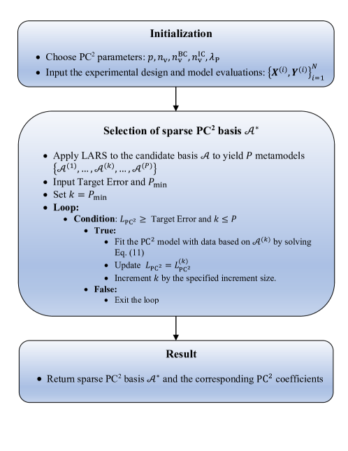
In sparse PC, for step 6 of the LARS procedure described above, leave-one-out cross-validation (LOOCV) is typically employed for each of the $P$ metamodels as an accuracy measure. This procedure is repeated by iteratively increasing the PCE order ($p$) and using heuristic criteria to check for overfitting, eventually yielding the best basis set corresponding to the best LOOCV. In contrast, the sparse PC ² implementation is simple and straightforward since it is robust to overfitting and provides better generalization error due to the integration of physical constraints. Therefore, there is typically no need to employ any cross-validation measure to evaluate the performance of the $P$ metamodels obtained from LARS and to implement specific criteria to prevent overfitting. The general rationale is that accuracy tends to improve with the addition of more basis functions (i.e., increasing $k$ basis functions) to train the PC ². We use the optimal value of the objective function, denoted as $L_{\textrm{\scalebox{1.05}{PC}${}^{2}$}{}}$, as a metric to evaluate the accuracy of the PC ² approximation. The computational flowchart of the proposed sparse PC ² is shown in Fig. 1. We began by specifying the tunable PC ² hyperparameters that are the $p$, $n_{v}$. We determine the value of $p$ by adjusting it based on the user-defined target error for the desired accuracy. Our empirical findings indicate that selecting a sufficiently large number of collocation points ensures a satisfactory fit. Additional increases do not offer further benefits in terms of numerical accuracy. After setting $p$ and the number of virtual collocation points, we input the ED and corresponding model evaluations ($\bm{Y}$). Based on $p$, we get the total number of basis functions as $P$ from Eq. (6). We then apply LARS, which gives $P$ metamodels $\left\{\pazocal{A}^{(1)},\ldots,\pazocal{A}^{(k)},\ldots,\pazocal{A}^{(P)}\right\}$ with increasing basis functions. As explained before, the accuracy of the PC ² generally improves as we incorporate more basis functions. So, we initiate $k=\pazocal{A}^{(P_{\text{min}})}$, where we specify $P_{\text{min}}$ denoting the minimum number of basis functions. We iterate $k$ from $\pazocal{A}^{(P_{\text{min}})}$ to $\pazocal{A}^{(P)}$ by incrementing $k$ by a fixed number at each step. For each step, we use the $k$ basis function to solve the optimization problem for PC ² coefficients and store the optimal value of the objective function, denoted as $L_{\textrm{\scalebox{1.05}{PC}${}^{2}$}{}}$. We terminate the procedure if the desired target error is met, i.e., $L_{\textrm{\scalebox{1.05}{PC}${}^{2}$}{}}<\text{Target error}$ and returns $\pazocal{A}^{*}$; otherwise, we continue to the next step.

3. Numerical results

In this section, we present numerical examples to demonstrate the capabilities of the proposed physics-constrained polynomial chaos expansion ( PC ²) in both SciML and UQ -related problems. We apply PC ² to diverse sets of problems, e.g., solving deterministic and stochastic PDEs, purely data-driven surrogate modeling of a physical system, and UQ of a stochastic system with parameters modeled as random fields. To solve the optimization problem for the PC ² coefficients (Eq. (18) and (21)), we use a quasi-Newton method, BFGS, as implemented in the SciPy library [45]. For standard unconstrained PCE , we use the UQ py library [46]. We utilize the Latin Hypercube Sampling (LHS) strategy [42] for sampling the virtual collocation points. All the computations are performed on an Apple M1 chip, 8-core CPU, and 8-core GPU, 16 GB RAM.

3.1 2D Heat Equation

This example aims to highlight the ability of our method to solve linear deterministic and stochastic PDEs. The 2D heat equation is a linear partial differential equation that describes how temperature evolves over time in a two-dimensional space. It is commonly used in physics and engineering to model heat conduction in various materials.

Consider the following 2D heat equation with the Neumann boundary condition as

$$\left\{\begin{array}[]{c}u_{t}-{\alpha}\left(u_{xx}+u_{yy}\right)=0,\quad x,y,t\in[0,1],\\ u\left(x,y,0\right)=0.5\left(\sin(4\pi x)+\sin(4\pi y)\right),\\ u_{x}\left(0,y,t\right)=0,\\ u_{x}\left(1,y,t\right)=0,\\ u_{y}\left(x,0,t\right)=0,\\ u_{y}\left(x,1,t\right)=0,\end{array}\right.$$ (27)

where $\alpha$ is the thermal diffusivity of the medium and $u$ is the 2D temperature field.

Figure 2: Comparison plots of

PC

² solution of the 2D heat Equation with the FEM solution at $t=1$, demonstrate a very good agreement between the two solutions.

We first consider a deterministic case with $\alpha=0.01$ and then extend it to a stochastic case. To compare the accuracy of the PC ² solution, we solve this problem numerically using the FEM with the FEniCS library [47].

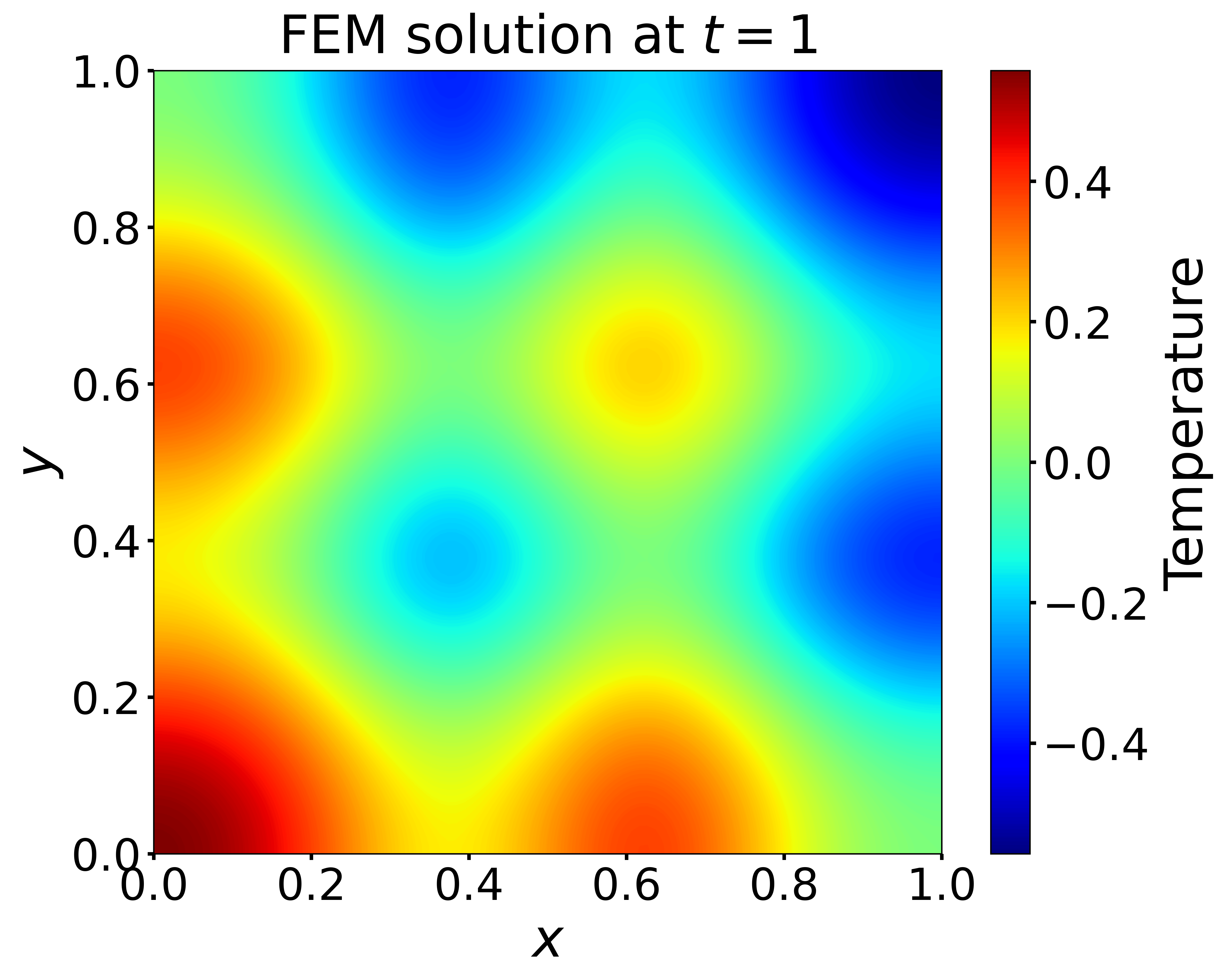
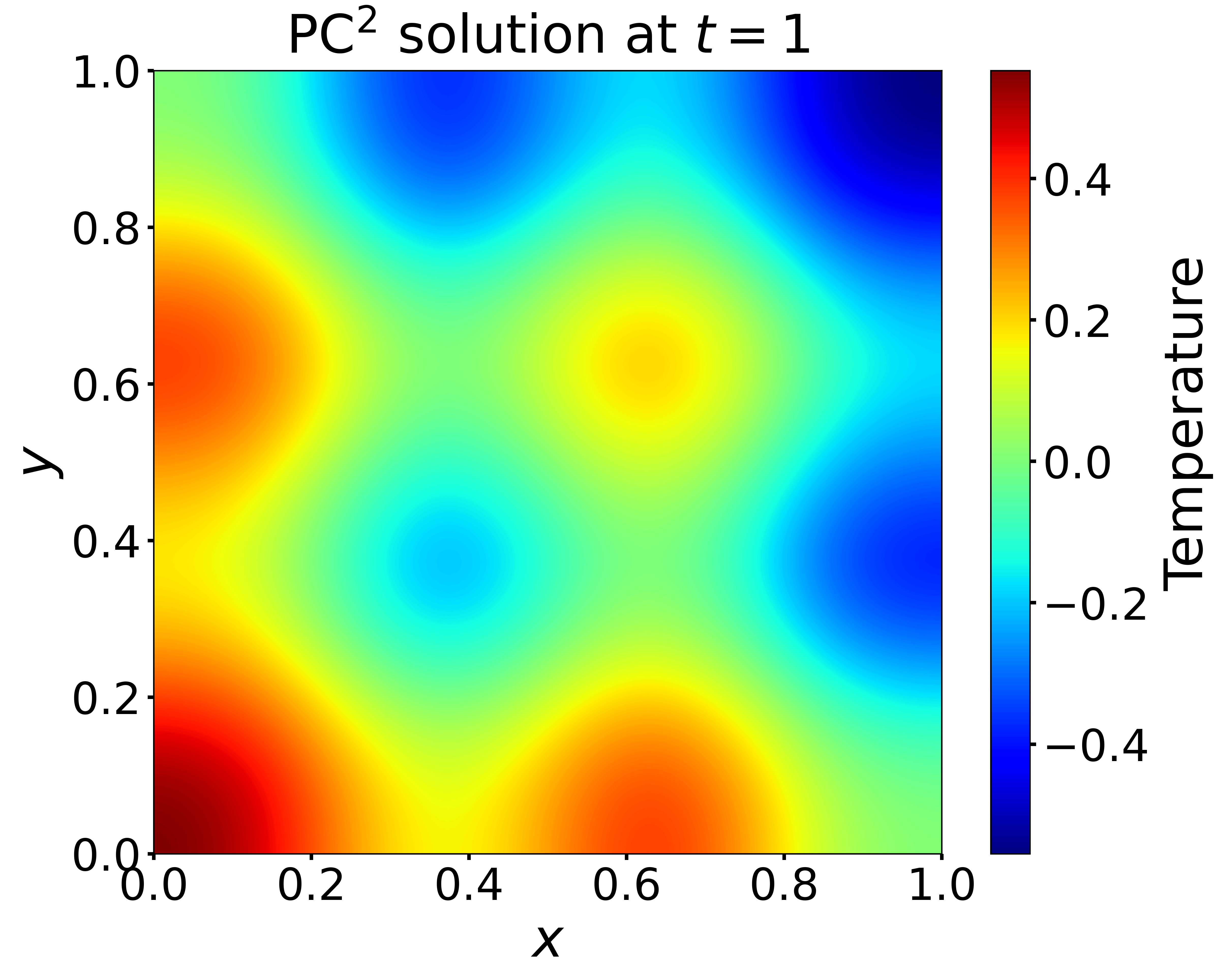
In the context of SciML for solving deterministic PDEs using PC ², we can incorporate training data in the form of experimental observations along with the PDE constraints enforced at virtual collocation points. This integration would otherwise be very difficult to achieve in standard PDE solvers, such as FEM. Also, we can incorporate low-fidelity numerical solutions (e.g., coarse-mesh FEM solution) to aid the training process. The training data activate sparse PC ² through LARS. It is also possible to train PC ² surrogate model without any labeled training data, similar to PINNs, where it works as a PDE solver. For this example, we use PC ² to solve the given PDE without any training data and enforce the PDE constraints using virtual collocation points taken as $n_{v}=5000,\ n_{v}^{\text{IC}}=200,\ n_{v}^{\text{BC}}=200$ with $p=10$. Figure 2 shows the plots of PC ² and the FEM solution at $t=1$. It can be observed that plot of the PC ² solution closely matches with the FEM solution. For the entire input domain discretized as $100^{3}$ points, we computed the mean square error (MSE) between PC ² and FEM solution. We get the MSE to be $1.53\times 10^{-04}$, which suggests a high numerical accuracy in the PC ² solution.

Now, to compare the performance of PC ² and sparse PC ² with standard sparse PCE based on least angle regression (LARS), referred to here as sparse PC, we plotted different MSEs with respect to increasing training samples in Figure 3. The $\text{MSE}_{\text{response}}$ corresponds to $u(x,\ y,\ t)$ as evaluated by PC ² and FEM, $\text{MSE}_{\text{physics}}$ corresponds to the residual based on given PDE and associated BC and IC. Their sum is represented as $\text{MSE}_{\text{total}}$. Since sparse PC and sparse PC ² are based on LARS, we need an experimental design or training data to perform feature selection using the LARS algorithm. We selected random points in the domain from the FEM solution for comparison with the sparse PC. Note that the standard PCE performance is notably poor, so it is not used for the comparison. In Figure 3, the dotted line represents the average MSE across 10 repetitions, while the shaded area around it encompasses the range from the minimum to the maximum MSE observed in the 10 repetitions. The minimum and maximum MSE represent a given method’s best and worst performance, respectively. As expected, the performance of PC ² is not influenced by the number of increasing domain samples since it already ensures that the given PDE is satisfied at virtual collocation points in the input domain. As described in Section 2.4, the sparse PC ² depends on the user-defined target error. The sparsity improves with the increasing number of domain samples, and the given target error is achieved with fewer polynomial basis functions. Consequently, it can be observed from Figure 3 that the MSE for both response and physics for sparse PC ² is close to the PC ² for the smaller number of domain samples, which means it needs a higher number of polynomial basis functions to achieve a given target error. However, as the number of training points increases, the sparsity improves, and sparse PC ² hits the target error with relatively fewer polynomial basis functions, ultimately converging to the PC ² solution. The MSEs for sparse PC decrease as the number of training points increases, and it takes around 200 points to give comparable performance as PC ² and sparse PC ² in terms of MSE response. However, the corresponding physics-based MSE is larger for all the training points considered, which suggests that for regions in input domains with fewer training data or complicated response surface, the sparse PC performs poorly in respecting the physics leading to an overall increase in the $\text{MSE}_{\text{physics}}$. As observed, the mean total MSE is the least for PC ², followed by sparse PC ² and sparse PC, suggesting the superior performance of the proposed method compared to standard PCE with minimal training data requirements.

Figure 3: 2D Heat Equation: Convergence plots of the different MSEs for

PC

², sparse

PC

² and sparse PC with respect to increasing training points. The $\text{MSE}_{\text{response}}$ and $\text{MSE}_{\text{physics}}$ is computed with respect to the FEM solution $u(x,\ t)$ and physics-based residuals associated with PDE, BC, and IC, respectively. $\text{MSE}_{\text{total}}=\text{MSE}_{\text{response}}+\text{MSE}_{\text{physics}}$. The dotted line indicates the average relative error, and the shaded area represents the minimum and maximum error across 10 repetitions.

Table 1: Comparison of different models in solving 2D Heat equation

Models	MSE at $t=1$	Training time (s)	Training data
PINNs [43]	$3.24\times 10^{-4}$	2259	746
PC 2	$6.36\times 10^{-5}$	232	0
Sparse PC 2	$6.42\times 10^{-5}$	21	746

The same 2D heat equation with the same initial and boundary conditions is also solved using PINNs in [43]. In Table 1, we showed the numerical accuracy and computational efficiency of the proposed full and sparse PC ² with that of PINNs, as reported in [43]. It can be observed that PC ² performs better than PINNs by providing an order of magnitude better accuracy in a fraction of the computational time without requiring any training samples, in contrast to the 746 samples used for PINNs. With the same training samples as PINNs, the sparse PC ² just takes 21 seconds to achieve the same level of accuracy as full PC ².

Having demonstrated the superior performance of the proposed method for SciML tasks, we now use the proposed method to solve the stochastic PDEs to integrate UQ , which is straightforward with PC ² in contrast to other SciML methods such as PINNs. In this case, we consider the stochastic 2D heat equation with parameter $\alpha$ modeled as a uniformly distributed random variable, $\alpha\sim\pazocal{U}[0.001,0.01]$. Again, in sharp contrast to standard PCE , it is possible to use PC ² to solve stochastic PDE without any model evaluations. Also, we get the output statistics for each point in the spatial and temporal domain in a single training, and the trained surrogate model conforms to the underlying PDE constraints for the entire physical and stochastic domain. Figure 4 shows the mean and standard deviation of the solution of stochastic 2D heat equation at $t=1$ using PC ² and Monte Carlo simulation (MCS), along with the respective absolute error. We use 10,000 model evaluations for MCS in contrast to zero model evaluations for PC ² to estimate the output statistics. The output statistics in terms of mean and standard deviation can be efficiently computed by post-processing the obtained PC ² coefficients (see Section 2.3). From Figure 4, it is evident that PC ² provides a reasonably good approximation of the moments for all the spatial points without needing any model evaluations.

Figure 4: UQ plots of the stochastic 2D heat equation: Top panel: Plots of the mean $u(x,\ y)$ at $t=1$ obtained by MCS and

PC

², along with their absolute error. Bottom panel: Plots of the standard deviation of $u(x,\ y)$ at $t=1$ obtained by MCS and

PC

², along with their absolute error. We used zero model evaluations to train the

PC

² surrogate model, in contrast, 10,000 model evaluations are used for MCS. The plots indicate an excellent performance of

PC

² in solving the stochastic 2D heat equation equation.

Table 2: Comparison of numerical accuracy and computational efficiency of

PC

² and sparse

PC

² in solving stochastic 2D Heat equation with respect to MCS.

Models	MAE of $\mu_{u}$	MAE of $\sigma_{u}$	Model	Training
	at $t=1$	at $t=1$	evaluations	time (s)
MCS	-	-	10000	56800
PC 2	0.004367	0.0047222	0	7800
Sparse PC 2	0.002308	0.003726	10	326

In Table 2, we demonstrate the performance of the proposed method in terms of numerical accuracy and computational time taken to solve the given stochastic PDE in comparison with the MCS. For the numerical accuracy, we use the mean absolute error (MAE) of $u$ at $t=1$ evaluated by taking an average of the absolute errors for each spatial point at $t=1$. It can be observed from Table 2 that high accuracy is achieved for the PC ² method even without taking any expensive model evaluations for training the surrogate model. PC ² takes a fraction of computational time in comparison to MCS. However, for this example, even though a desirable accuracy can be reached at a lower PCE order ($p$) with significantly less computational time, we deliberately consider a higher order $p=10$, which corresponds to 1001 polynomial basis functions, to show its comparison with sparse PC ². For this problem, the PC ² is over-parameterized with many redundant polynomial basis functions. From Table 2, we can see that considering only a few model evaluations activates the sparse PC ², which significantly reduces the total polynomial basis by providing only the most influential polynomial basis. Consequently, the computational time is drastically reduced compared to PC ², with also a significant improvement in the numerical accuracy, which is credited to a much simpler optimization process with a few coefficients to compute in comparison to PC ². This shows the superior performance of the proposed sparse PC ² representation in solving the stochastic PDE.

3.2 Burgers’ Equation

This example aims to highlight the ability of our method to solve non-linear deterministic and stochastic PDEs. The 1D viscous Burgers’ equation is a non-linear partial differential equation that describes the behavior of viscous fluid flow. Consider the following 1D viscous Burgers’ equation with the Dirichlet boundary condition as

$$\left\{\begin{array}[]{c}u_{t}+uu_{x}=\nu u_{xx},\quad x\in[0,1],t\in[0,0.3],\\ u\left(x,0\right)=\sin(\pi x),\\ u\left(0,t\right)=0,\\ u\left(1,t\right)=0,\\ \end{array}\right.$$ (28)

where $\nu$ is the fluid viscosity and $u$ represents the fluid velocity.

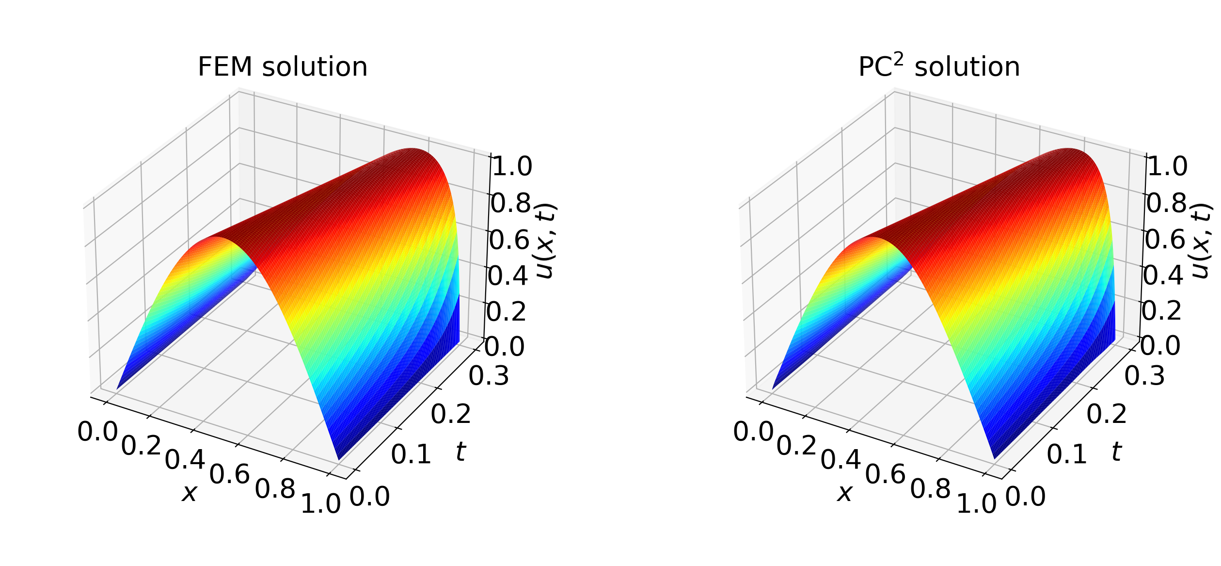
Similar to the previous example, we first consider a deterministic case with $\nu=0.001$ and then extend it to the stochastic case. Again, we first solve this equation numerically using FEM with the FEniCS library [47] to compare the accuracy of the PC ² solution. For this example, we take $p=20$ and the number of virtual collocation points as $n_{v}=2000,\ n_{v}^{\text{IC}}=100,\ n_{v}^{\text{BC}}=100$. As in the previous example, no labeled training data is used to train the PC ² surrogate model. Figure 5 shows the plots of PC ² and the FEM solution for the given input domain. It is evident that the PC ² provides an excellent approximation compared to the FEM solution, which suggests the effectiveness of the proposed method in solving non-linear PDEs. Table 3 shows the relative numerical accuracy and the computational efficiency of the full and sparse PC ² compared to the FEM solution. The results show excellent numerical accuracy with high computational efficiency for the proposed method.

(a)

(b)

Figure 5: Comparison plots of

PC

² solution of the Burgers’ Equation with the FEM solution demonstrate a very good agreement between the two solutions.

Table 3: Comparison of

PC

² and sparse

PC

² models in solving Burgers’ equation.

Models	MSE	Training time (s)	Training data
PC 2	$4.54\times 10^{-5}$	68	0
Sparse PC 2	$3.33\times 10^{-4}$	15	500

Figure 6: Burgers’ Equation: Convergence plots of the different MSEs for

PC

², sparse

PC

² and sparse PC with respect to increasing training points. The $\text{MSE}_{\text{response}}$ and $\text{MSE}_{\text{physics}}$ is computed with respect to the FEM solution $u(x,\ t)$ and physics residuals associated with PDE, BC, and IC, respectively. $\text{MSE}_{\text{total}}$=$\text{MSE}_{\text{response}}+\text{MSE}_{\text{physics}}$. The dotted line indicates the average relative error, and the shaded area represents the minimum and maximum error across 10 repetitions for each training point.

Again, to compare the proposed method with standard sparse PC, we plotted the different MSE for PC ², sparse PC ², and sparse PC against training samples in Figure 6. The convergence trends of the compared methods are similar to the previous example with a notably poor performance by sparse PC for $\text{MSE}_{\text{physics}}$, which is expected since the problem is non-linear and is difficult to approximate. The sparse PC is unable to capture the non-linearity as $t$ increases, which results in an overall increase of the $\text{MSE}_{\text{physics}}$. On the other hand, the performance of PC ² and sparse PC ² are significantly better, as suggested by the plots of $\text{MSE}_{\text{total}}$. This indicates that the proposed method is capable of accurately capturing the complexity of the response $u$ with time. However, it is worth mentioning that with the evolution of the response with time, the solution becomes non-differentiable, which is difficult to approximate using polynomials. Hence, there is a limit in time $t$ for which the proposed method provides an accurate approximation for non-linear PDEs. There are possible ways to mitigate this issue by adopting domain adaptive local PCE [48] for PC ², which is a subject of further work. Nevertheless, the performance is significantly superior to the standard PCE .

Now, we consider the stochastic case with $\nu\sim\pazocal{U}[0.001,0.1]$. Figure 7 shows the mean and standard deviation of the solution of stochastic 1D Burgers’ equation using PC ² and MCS, along with the respective absolute error. Again, we have not taken any expensive model evaluations to train the surrogate model. From Figure 7, it is evident that PC ² provides a reasonably good approximation of the moments without needing any model evaluations in contrast to 10,000 model evaluations for MCS. In Table 4, we show the numerical accuracy and computational efficiency of the proposed method in comparison with MCS. Again, for this example, we considered a high PCE order $p=18$ (corresponding to 1330 polynomial basis) to most accurately estimate the output statistics and to compare the PC ² with the sparse PC ². As can be observed from Table 4, the sparse PC ² achieves excellent accuracy in estimating the mean and standard deviation compared to MCS with substantial computational time saving by utilizing just a few model evaluations. The PC ² is over-parameterized for this case, and hence it takes considerable time compared to sparse PC ² to converge to the solution, but still significantly less than the MCS.

Figure 7: UQ plots of the stochastic Burgers’ equation: Top panel: Plots of the mean $u(x,\ t)$ obtained by MCS and

PC

², along with their absolute error. Bottom panel: Plots of the standard deviation of $u(x,\ t)$ obtained by MCS and

PC

², along with their absolute error. We used zero model evaluations to train the

PC

² surrogate model, in contrast, 10,000 model evaluations are used for MCS. The plots indicate an excellent performance of

PC

² in solving the stochastic Burgers’ equation.

Table 4: Comparison of numerical accuracy and computational efficiency of

PC

² and sparse

PC

² in solving stochastic Burgers’ equation with respect to MCS.

Models	MAE of $\mu_{u}$	MAE of $\sigma_{u}$	Model evaluations	Training time (s)
MCS	-	-	10000	62400
PC 2	$1.06\times 10^{-3}$	$1.09\times 10^{-3}$	0	13800
Sparse PC 2	$4.39\times 10^{-3}$	$5.04\times 10^{-3}$	50	960

(a)	(b)
(c)	(d)

Figure 8: Comparison plots of the EOS surrogate model based on

PC

² and

PCE

with regions of constraint violations represented by red. (a) Pressure

PC

² EOS surrogate model. (b) Energy

PC

² EOS surrogate model. (c) Pressure

PCE

EOS surrogate model. (d) Energy

PCE

EOS surrogate model. The

PC

² surrogate models provide an improved fit with respect to the validation data without violating the thermodynamic constraints.

3.3 Data-driven surrogate modeling: Equation of state models

The purpose of this example is to highlight the effectiveness of using PC ² in a purely data-driven setting where the computational model is prohibitively expensive or when dealing with experimental data. This is typically the case where we have some observational data and some understanding of the fundamental underlying physics. Here, we take an example of an equation of state (EOS) model. EOS models provide a mathematical relationship between a material’s thermodynamic properties, such as pressure, internal energy, temperature, and density. EOS models are essential for closing the conservation equations of mass, momentum, and energy in hydrodynamic simulations, which are used across various branches of physics, engineering, and chemistry to describe and predict the behavior of materials under different conditions. EOS models are typically constructed using a semi-empirical parametric methodology, which assumes a physics-informed functional form with many tunable parameters that are calibrated using a complex combination of experimental and first-principles simulation data from a variety of sources. Recently, there have been efforts to replace this approach with a purely data-driven approach using ML [5]. However, in the data-driven setting, the EOS surrogate model must satisfy the fundamental laws of thermodynamics necessary to be useful in hydrocode simulation. The EOS surrogate model must obey the thermodynamic stability constraints, which are derived from the second law of thermodynamics and are given as

$$\left(\frac{\partial^{2}F}{\partial V^{2}}\right)_{T} =-\left(\frac{\partial P}{\partial V}\right)_{T}=\frac{1}{V\kappa_{T}}\geq 0\Longleftrightarrow\kappa_{T}>0\Longleftrightarrow\left(\frac{\partial P}{\partial V}\right)_{T}\leqslant 0,$$ (29)

$$\left(\frac{\partial^{2}S}{\partial E^{2}}\right)_{V} =-\frac{1}{T^{2}}\left(\frac{\partial T}{\partial E}\right)_{V}=-\frac{1}{T^{2}c_{\nu}}\leqslant 0\Longleftrightarrow c_{V}>0\Longleftrightarrow\left(\frac{\partial E}{\partial T}\right)_{V}\geqslant 0,$$ (30)

where $F,\ S$ are the Helmholtz free energy and entropy, respectively. $P,\ E$ are the pressure and internal energy, respectively, which are the outputs of the EOS surrogate model. $V,\ T$ are the volume and temperature, respectively, taken as inputs. And, $\kappa_{T}$ and $c_{V}$ are isothermal compressibility and specific heat, respectively, which should remain positive for all the EOS predictions.

(a)
(b)

Figure 9: Histograms of relative $\pazocal{L}^{2}$-norm error and percent constraint violations for

PC

² and

PCE

surrogate models with respect to 100 training datasets with randomly selected 8 points from the given 96 DFT-MD data. (a) $\pazocal{L}^{2}$-norm error for pressure EOS and energy EOS, showing more datasets with low relative error for

PC

² compared to

PCE

. (b) Constraint violation ($\%$) for pressure EOS and energy EOS, showing all datasets satisfy the constraints for

PC

² compared to many datasets violating constraints for

PCE

. $\pazocal{L}^{2}$-norm error is calculated for each training dataset with respect to the complementary validation dataset. Constraint violation is the fraction of the number of test points violating the constraints.

(a)	(b)
(c)	(d)

Figure 10: Comparison plots of the EOS surrogate model based on

PC

² and

PCE

with Gaussian noise added to the output observations of the training data. (a) Mean pressure

PC

² EOS. (b) Mean energy

PC

² EOS. (c) Mean pressure

PCE

EOS. (d) Mean energy

PCE

EOS. Colors denote the standard deviation of the model at each point. The mean

PC

² surrogate models provide an improved fit with respect to the validation data with significantly less standard deviation compared to

PCE

, indicating enhanced robustness in handling noise in the training data. We added Gaussian noise with zero mean and standard deviations of 5 GPa and 0.5 ev/atom independently to each training observation of the pressure and energy data, respectively.

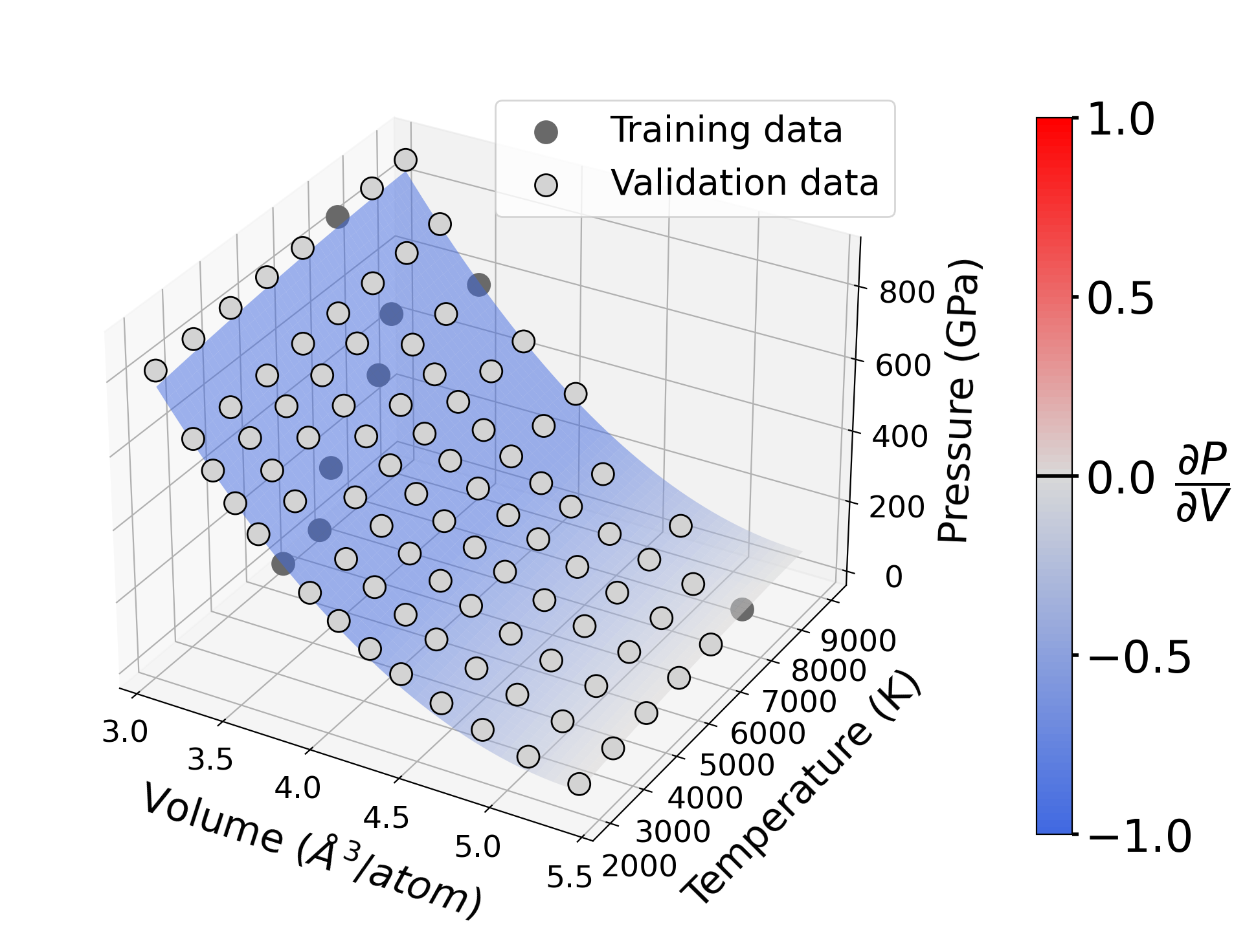
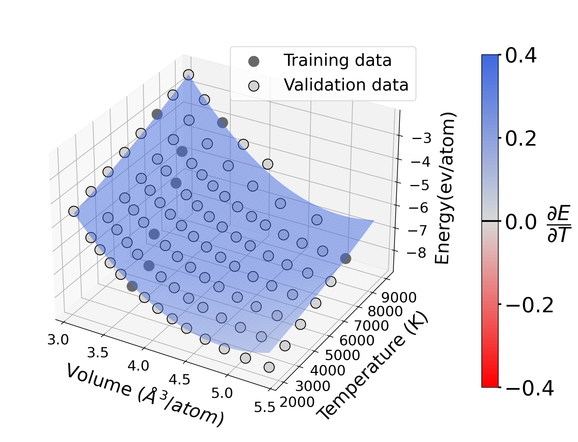
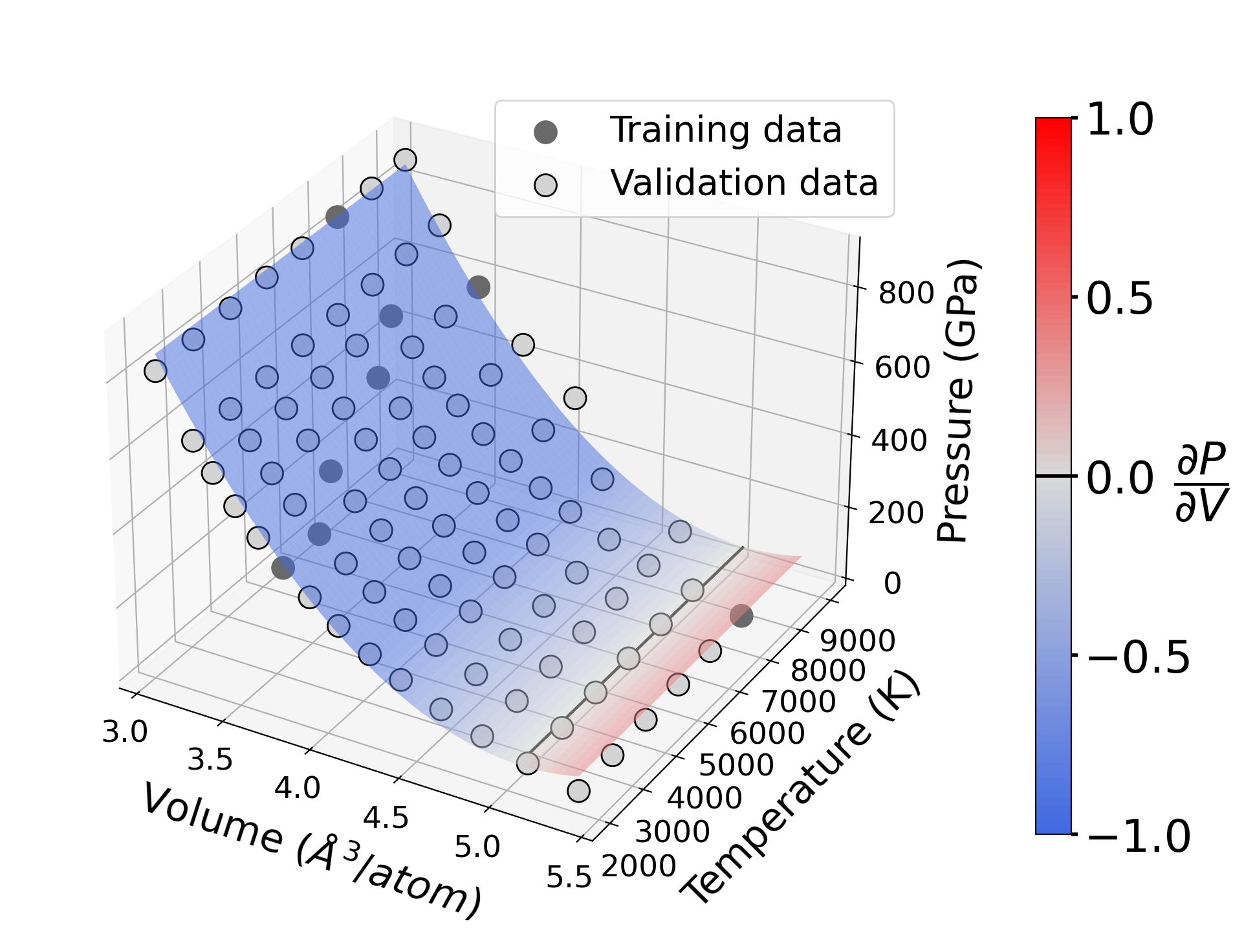
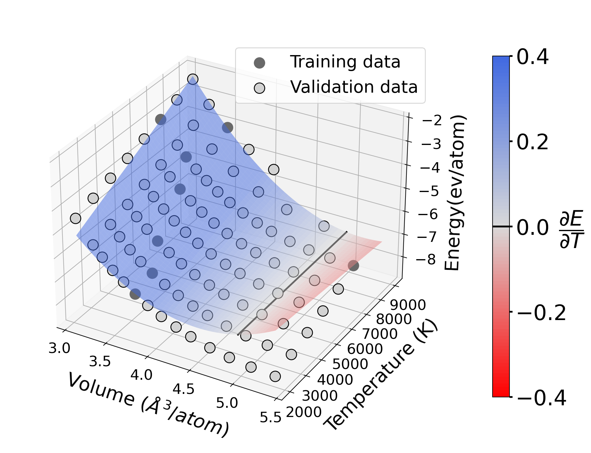
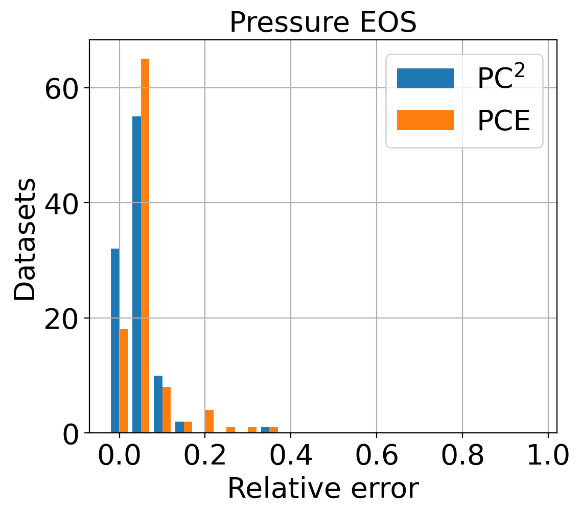
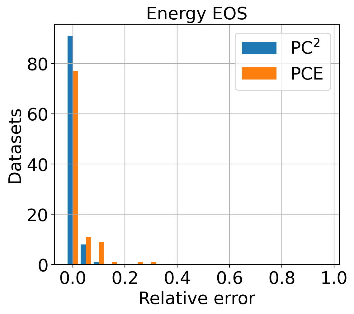
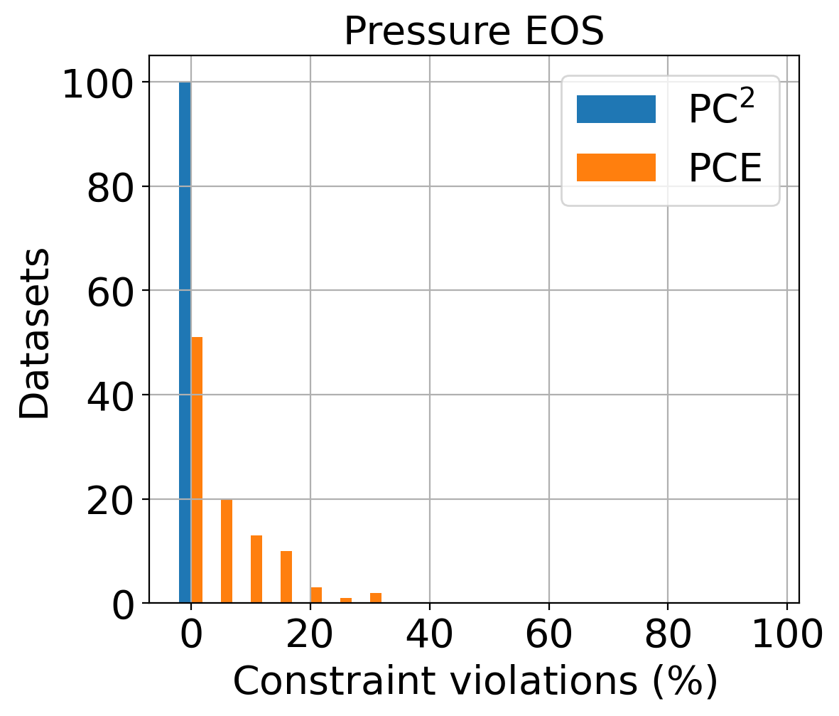
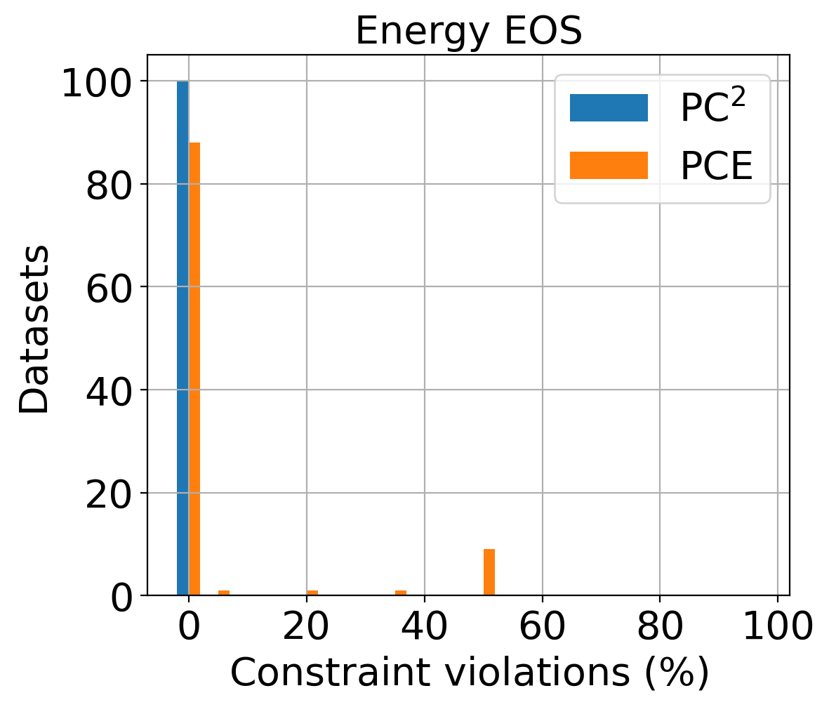
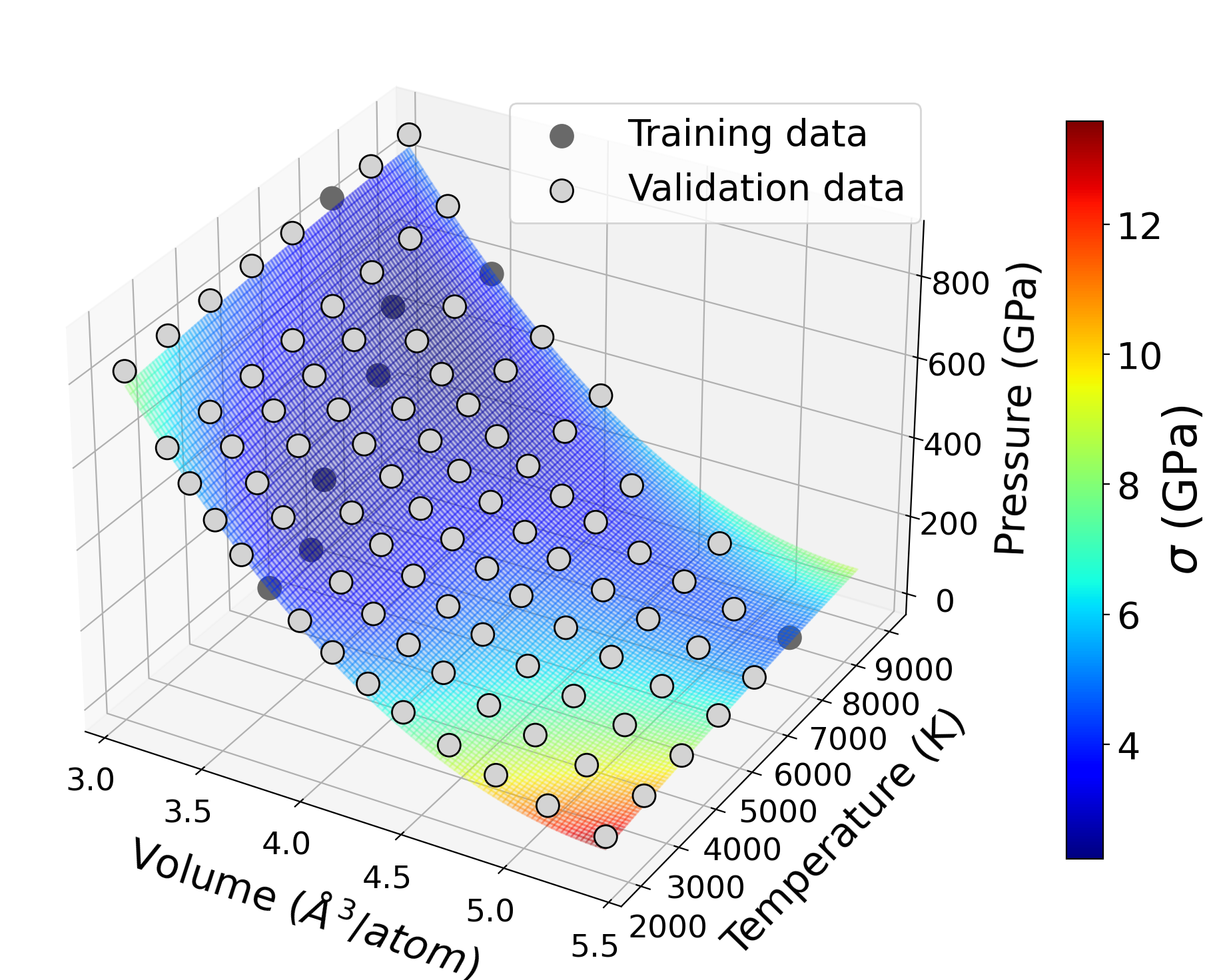
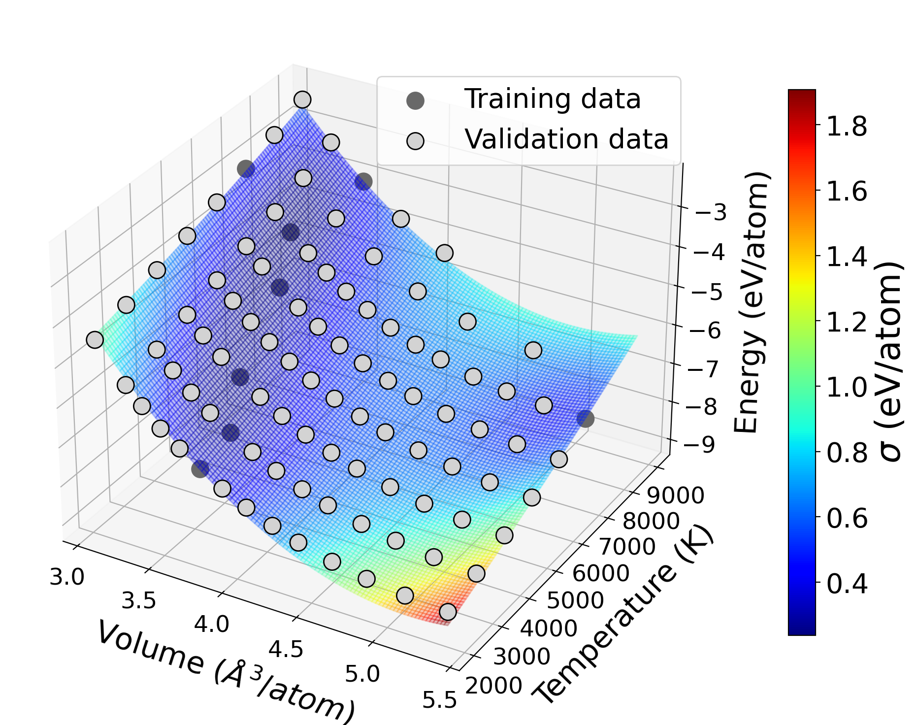
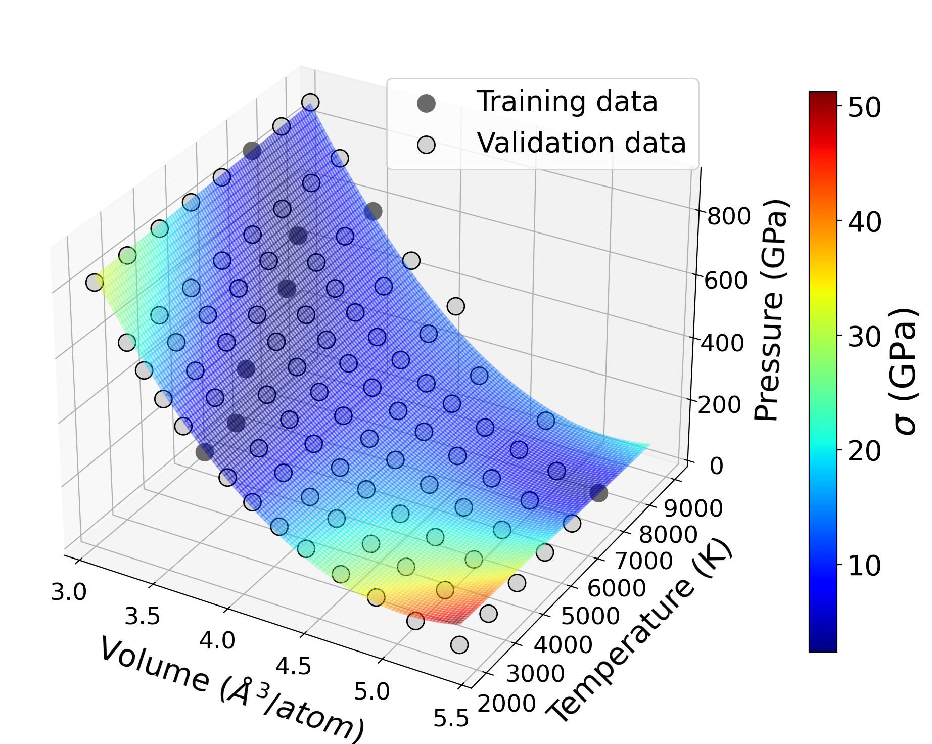
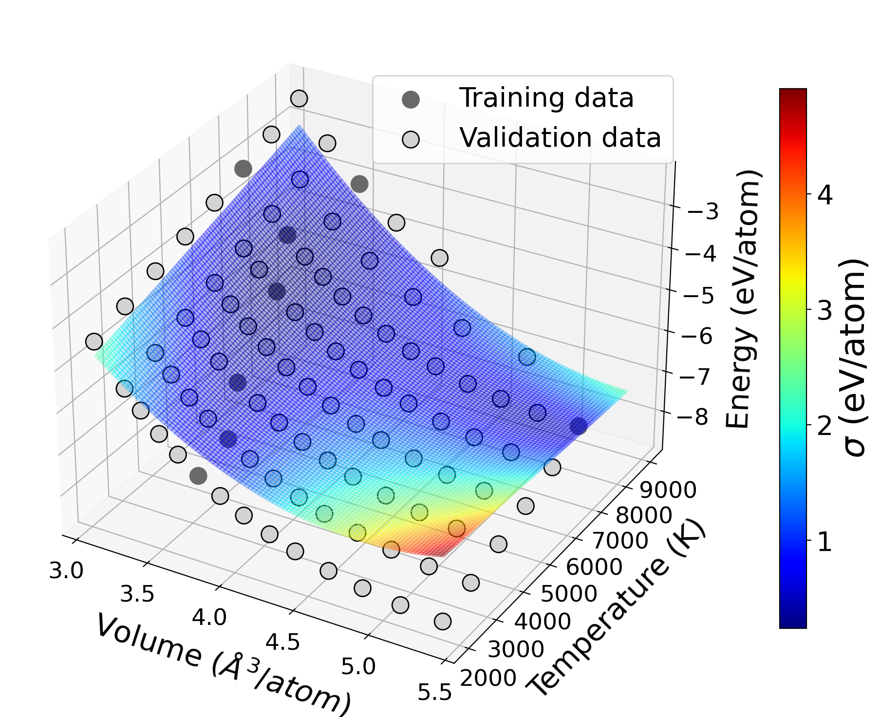
In the present context, we would like to use the proposed PC ² as a data-driven surrogate model while ensuring that the model satisfies the fundamental thermodynamical laws. For this example, we use data points from Density Functional Theory Molecular Dynamics (DFT-MD) simulations for diamond from Benedict et al. [49] for the training process. The EOS model outputs pressure and internal energy for a given input of volume and temperature. We have 96 data points, which we split into training and validation sets of 8 and 88 points, respectively. Figures 8 (a) and (b) show the pressure and energy PC ² surrogate model as a function of state variables $(V,T)$, respectively, trained from 8 data points, with color bars representing the constraints violations. We enforce the constraints at 600 virtual collocation points in the input domain. We similarly trained using the standard PCE surrogate model in Figures 8 (c) and (d). It can be clearly observed that the PC ² provides a better fit for both pressure and internal energy with respect to the validation set compared to unconstrained PCE . Also, it is evident from the figures that the proposed PC ² surrogate model satisfies the constraints at every point in the input domain. However, the standard PCE surrogate model violates both constraints at many points, which suggests physically unrealistic predictions, making it impractical to use in hydrocode simulations. To demonstrate the robustness of the PC ² model, we created 100 datasets with randomly selected 8 training points and complementary validation set from the given 96 DFT-MD points and trained the proposed PC ² and PCE surrogate model for each dataset. For each trained model, we reported the relative $\pazocal{L}^{2}$-norm error with respect to the respective validations set and the percentage of constraint violations and plotted the histograms in Figure 9. As can be seen from Figure 9 (a), the histograms are weighted more toward the lower relative error for PC ², which suggests an improved fit compared to PCE . Also, from Figure 9 (b), the constraints are not violated for any datasets for PC ², whereas the constraints violations are high for many datasets for the PCE surrogate model. These plots indicate superior performance of PC ² in a data-driven setting compared to PCE .

Furthermore, we study the behavior of the proposed PC ² surrogate model in handling the noise compared to PCE by adding Gaussian noise to each output’s observations in the training dataset. The model is retrained based on the perturbed outputs, and the predictions are ensembled to compute the statistics [28]. Figure 10 shows the plot of the PC ² and PCE mean and standard deviation for pressure and internal energy against volume and temperature. It can be observed that the mean response surface for PC ² provides a better fit with respect to validation data points for each output compared to PCE , even in the case of noisy outputs in the training dataset. Moreover, the standard deviation of the PC ² response for each output is significantly lesser than the PCE , which suggests enhanced robustness in handling noise in the training data. As expected, the standard deviation is observed to be higher in the regions where the training data is not present. The superior performance of the proposed method in a data-driven setting is attributed to the incorporation of physical constraints, which enriches the limited training data and provides realistic predictions.

3.4 Stochastic Euler Bernoulli beam

In this example, we utilize the PC ² surrogate model in a standard UQ setting where PCE is generally employed. The objective of this example is to compare the performance of the proposed PC ² method with the standard sparse PCE in UQ of physical systems and to test the performance of the proposed method for high-dimensional problems. Here, we apply PC ² to perform the uncertainty quantification of an Euler Bernoulli (EB) beam with Young’s modulus ($E$) modeled as 1D Gaussian random field with exponential covariance kernels; $C(x_{1},x_{2})=\sigma^{2}\exp(-|x_{1}-x_{2}|/l_{c})$, where $\sigma$ is the standard deviation, $x_{1}$ and $x_{2}$ are the coordinates along the length of the beam and $l_{c}$ is the correlation length of the random field. The Karhunen-Loève expansion [15] is employed to discretize the random field.

Figure 11: Simply supported Euler Bernoulli beam.

Figure 12: Plot of eigenvalues decay with respect to the number of KL terms, indicating 7 KL terms are sufficient to capture the stochasticity of the random field.

(a)

(b)

(c)

Figure 13: (a) Plot of the mean deflection along the length of the beam estimated by MCS,

PC

² and sparse

PC

². (b) Plot of the standard deviation of the deflection along the length of the beam estimated by MCS,

PC

² and sparse

PC

². (c) Plot of the probability density function of the midpoint deflection estimated by MCS,

PC

² and sparse

PC

². All the plots indicate good convergence of

PC

² and sparse

PC

² in estimating the response statistics in comparison to MCS. We used zero model evaluations for

PC

², 100 model evaluations for sparse

PC

², and 100,000 model evaluations for MCS with $\text{COV}=5\%$.

A simply supported Euler Bernoulli beam of length $L$ with uniformly distributed load $q$, is shown in Figure 11. The bending behavior of the EB beam is governed by the following equation:

$$\frac{\mathrm{d}^{2}}{\mathrm{~{}d}x^{2}}\left(EI\frac{\mathrm{d}^{2}w}{\mathrm{~{}d}x^{2}}\right)=q,$$ (31)

where $w$ denotes the lateral deflection, and $I$ is the second moment of area of the beam’s cross-section.

The KL expansion discretization for the $E$ random field is given as

$$E(\mathbf{x},\theta)={\overline{E}}+\sum_{i=1}^{r}\sqrt{\lambda_{i}}\phi_{i}(\mathbf{x})\xi_{i}(\theta),$$ (32)

where ${\overline{E}}$ is the mean of the random field, $\left(\lambda_{i},\phi_{i}\right)$ are the eigenpairs, and $\xi_{i}(\theta)$ is a set of independent standard Gaussian random variables, and $r$ represents the KL terms.

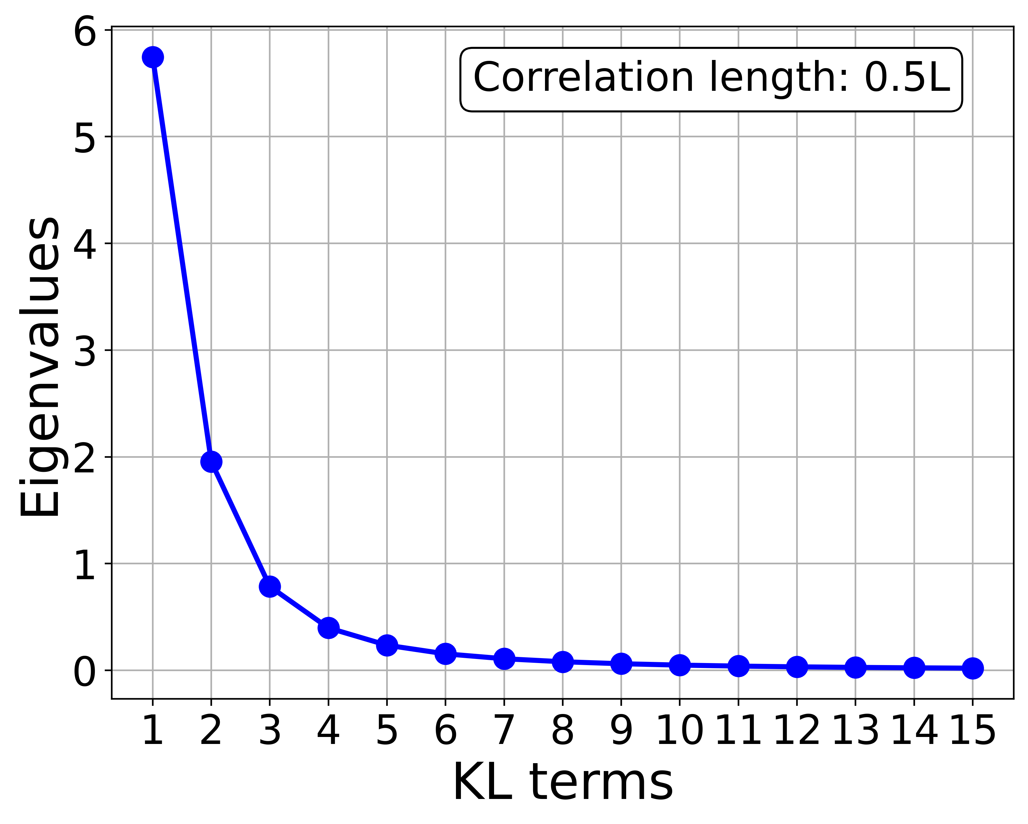
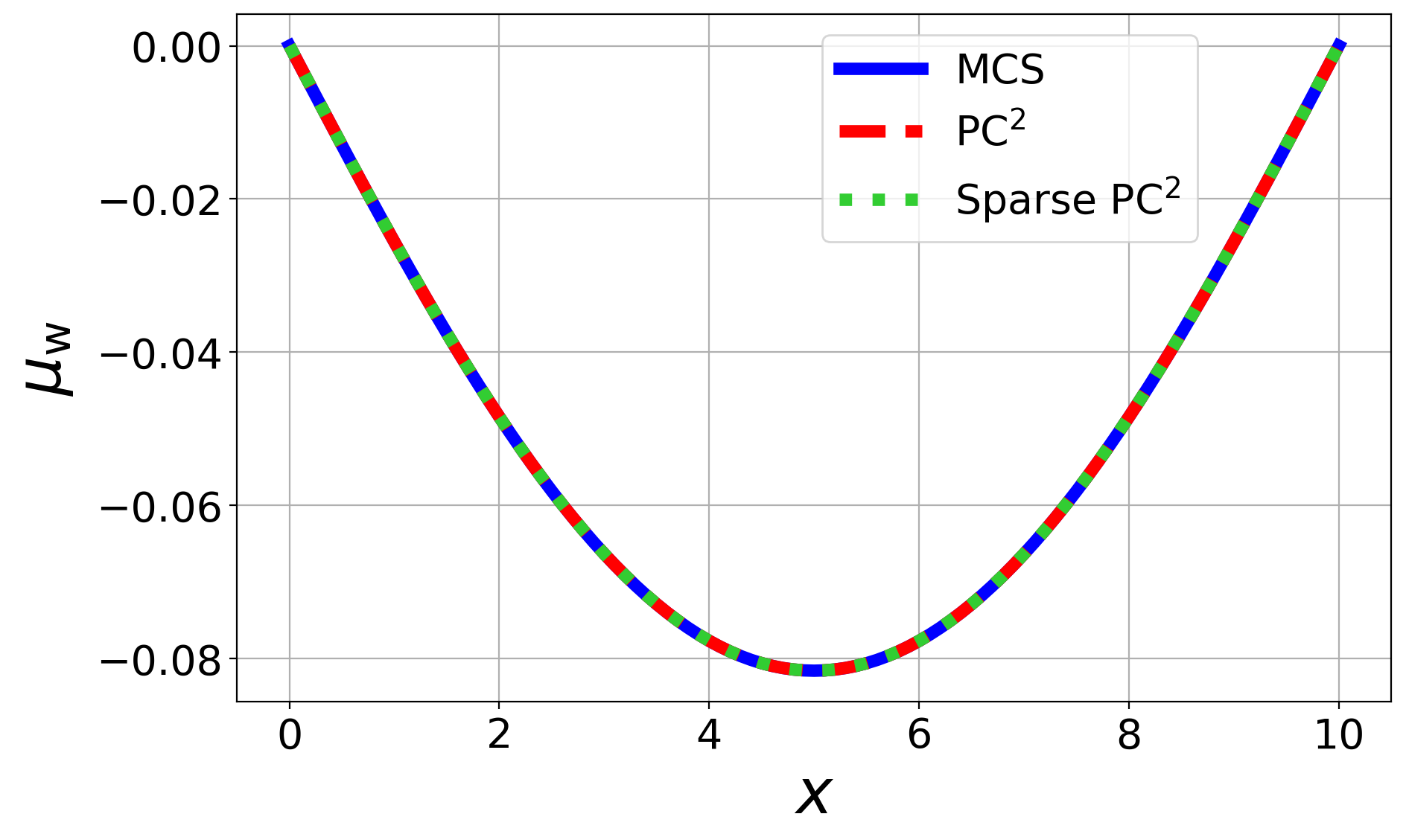
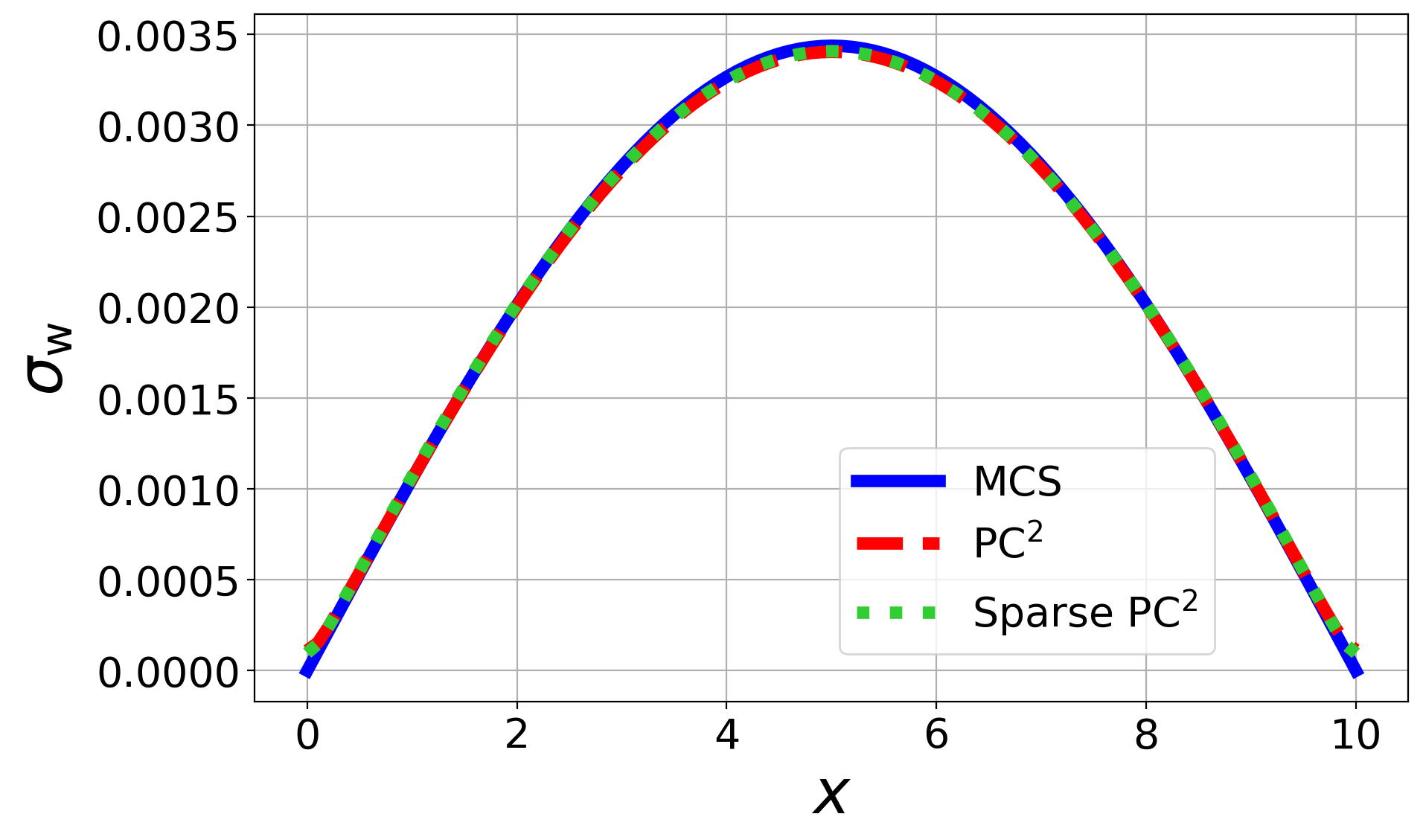
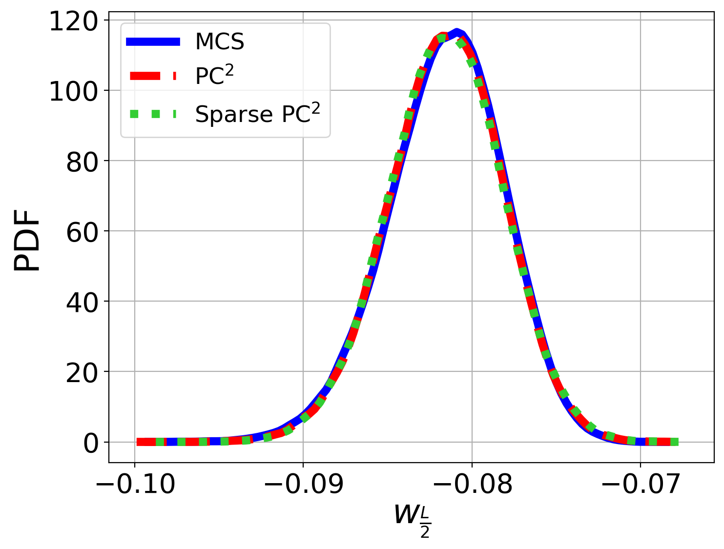
For computations, we considered $L=10\ m$, $q=-5\ kN/m$, $I=10^{-4}\ m^{4}$, and ${\overline{E}}=80\ GPa$. Figure 12 shows the plot for the eigenvalue decay with respect to the number of KL terms for a correlation length $l_{c}=0.5L$. As can be observed, 7 KL terms are sufficient to capture the stochastic behavior of the underlying random field. For this example, we have taken $p=5$ and the number of virtual collocation points as $n_{v}=20000,\ n_{v}^{\text{BC}}=5000$ for physical and stochastic dimensions. Figure 13 (a) and (b) shows the plots for the mean and standard deviation of the beam’s deflection $w$ as a function of $x$ computed using PC ², sparse PC ² and MCS. For training the surrogate models, we used zero model evaluation for PC ² and 100 model evaluations for sparse PC ², compared to 100,000 for MCS. The plots show that the proposed PC ² provides an excellent statistical approximation of both mean and standard deviation across $x$ compared to MCS. Figure 13 (c) shows the plot of the probability density function (pdf) of midpoint deflection estimated using PC ², sparse PC ², and MCS. Notably, there is a good convergence among the PDFs, indicating superior performance in capturing the stochasticity of the response. Also, it can be observed from the figures that the numerical accuracy is similar for both the PC ² and sparse PC ²; however, the sparse PC ² took only 25 seconds compared to 1440 seconds for PC ² to train, which shows significant computational savings for sparse PC ². Hence, it is recommended to use sparse PC ² when dealing with high-dimensional problems.

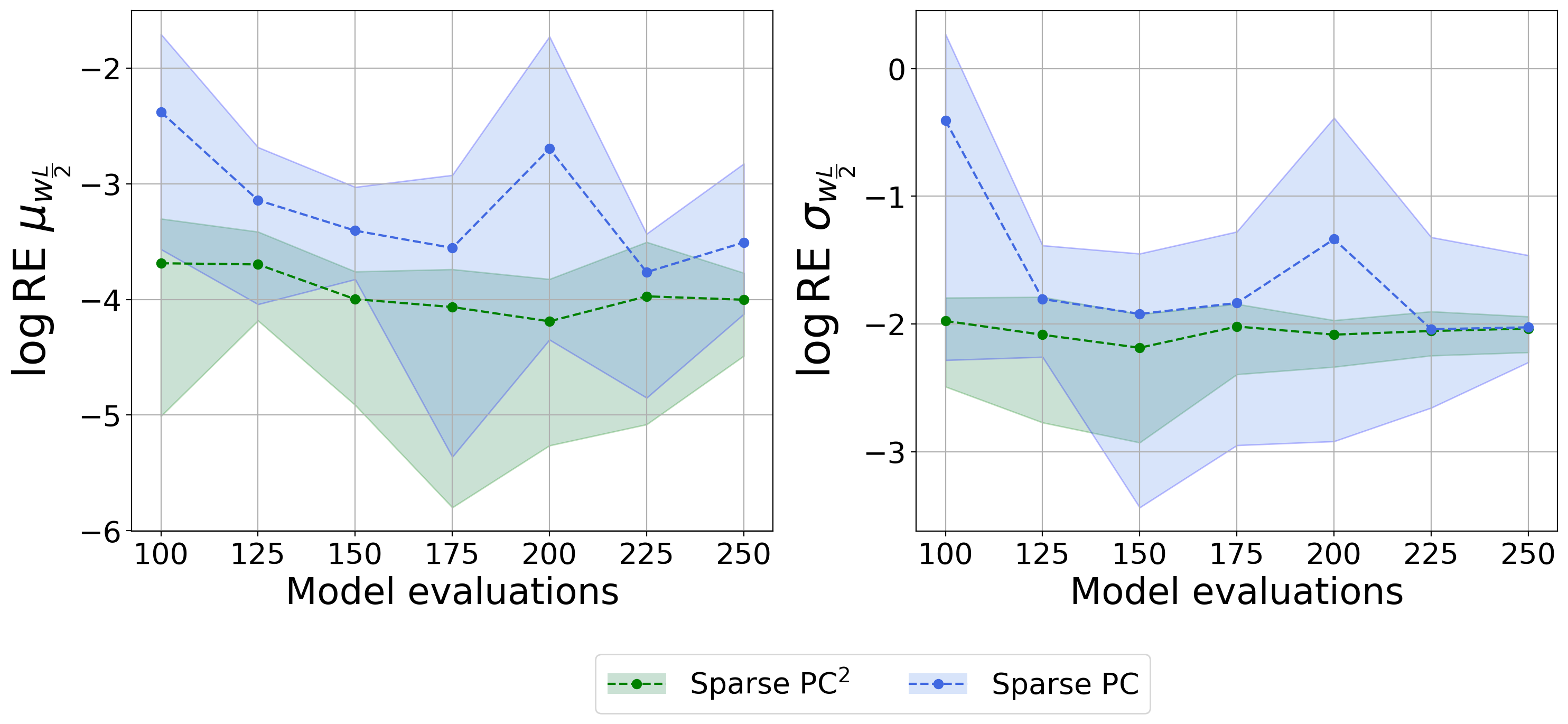
Now, to compare the performance of sparse PC ² with sparse PC, we computed the relative error in mean and standard deviation of the mid-point deflection for PC ² and sparse PC with respect to MCS. To check the robustness of performance, we retrained both surrogate models 10 times for each model evaluation with ED based on LHS sampling. We plotted the results in Figure 14, with dotted lines representing the average RE and the shaded area representing the range from the minimum to the maximum RE, as observed in the 10 repetitions. It can be observed from the figure that the sparse PC ² provides improved performance in terms of the average relative error for both mean and standard deviation. From the minimum and maximum relative errors, it can be inferred that the sparse PC ² is less sensitive to the sampling of ED, which is expected since the ED is enriched by physical constraints, and provides a consistent performance for all the model evaluations considered. On the other hand, sparse PC is sensitive to the sampled points in ED, especially for lower model evaluations, and the performance improves with increasing model evaluations. Also, the maximum relative error for sparse PC ² is much less than the sparse PC, suggesting reliable estimations of the moments for sparse PC ². This demonstrates the superior performance of the proposed surrogate method in the reliable and robust uncertainty assessment of stochastic systems with fewer model evaluations.

To test the computational performance of the proposed sparse PC ², we further increased the stochastic dimensionality by considering 10, 15, and 20 KL terms, with $p=5$ and one physical variable, which corresponds to 4368, 20349, and 65780 polynomial basis, respectively. We considered 300 model evaluations for training the surrogate model for each case and reported the computational time and mean and standard deviation of midpoint deflection estimated by sparse PC ² and MCS in Table 5. It can be observed from the table that the sparse PC ² provides an excellent computational performance for high stochastic dimensionality problems taking only a few minutes to achieve a given target error, which can be observed based on the accuracy of estimated mean and standard deviation compared to MCS. This improvement is attributed to the simplified sparse implementation and the incorporation of physical constraints. Despite a very high number of polynomial basis, only a few hundred contribute most to the output response, which are effectively identified by the sparse PC ² through LARS. This indicates that the proposed method is suitable for efficient and reliable UQ of stochastic systems with high stochastic dimensionality. However, it is worth mentioning that the performance of sparse PC ² depends on the effectiveness of LARS to provide the most influential polynomial basis, which generally improves with increasing model evaluations. For cases with insufficient model evaluations, the sparse PC ² may require more polynomial basis to achieve a given target error, resulting in an increased computational cost.

Figure 14: Comparison plots of the relative error of the mean and standard deviation of midpoint deflection estimated using sparse

PC

² and sparse PC with respect to MCS against the increasing model evaluations. The dotted line indicates the average relative error, and the shaded area represents the minimum and maximum error across 10 repetitions for each model evaluation.( $\text{COV}=10\%$)

Table 5: Computational performance of sparse

PC

² for $\text{COV}=10\%$ with 300 model evaluations used for training.

KL terms	$l_{c}$	Polynomial	Training	Sparse PC 2		MCS
		basis	time (s)	$\mu_{w_{0.5L}}$	$\sigma_{w_{0.5L}}$	$\mu_{w_{0.5L}}$	$\sigma_{w_{0.5L}}$
10	$0.3L$	4368	26	-0.08213708	0.00627731	-0.08215744	0.00638659
15	$0.2L$	20349	95	-0.08211130	0.00564987	-0.08216044	0.00574360
20	$0.1L$	65780	382	-0.08202917	0.00447343	-0.08212911	0.00411479

4. Conclusion

In this work, we have proposed a novel physics-constrained polynomial chaos surrogate model that integrates physical knowledge in the polynomial chaos framework. The incorporation of physical constraints in the training process effectively reduces the need for expensive model evaluations and ensures physically realistic predictions. The proposed method is capable of addressing problems related to scientific machine learning and uncertainty quantification, which we have demonstrated through various numerical examples. In the scientific machine learning domain, the proposed method is well suited for problems with some data and a partial understanding of the underlying physics and features a built-in uncertainty quantification capability. In uncertainty quantification domains, the incorporation of physics constraints enriches the experimental design, enhancing the accuracy of uncertainty assessment. Further, we proposed a sparse implementation to handle high-dimensional problems in the polynomial chaos context, which showcases excellent performance in dealing with high-dimensional stochastic problems. The proposed method demonstrates promising results for a wide range of problems with superior performance in numerical accuracy and computational efficiency. However, the method is only suited for sufficiently smooth responses. Extension to non-smooth problems is possible with local PCE [48], which is a subject of future research. Also, a more rigorous testing of the proposed method in handling practical problems is an area for further investigation.

5. Acknowledgements

This work was supported by the Defense Threat Reduction Agency, Award HDTRA12020001. LN gratefully acknowledges support of the Czech science foundation under project No. 23-04974S. The international collaboration was supported by the Ministry of Education, Youth and Sports of the Czech Republic under project No. LUAUS24260.

References

- [1] J. Kudela and R. Matousek, “Recent advances and applications of surrogate models for finite element method computations: A review,” Soft Computing, vol. 26, no. 24, pp. 13709–13733, 2022.
- [2] H. Liu, Y.-S. Ong, and J. Cai, “A survey of adaptive sampling for global metamodeling in support of simulation-based complex engineering design,” Structural and Multidisciplinary Optimization, vol. 57, pp. 393–416, 2018.
- [3] J. N. Fuhg, A. Fau, and U. Nackenhorst, “State-of-the-art and comparative review of adaptive sampling methods for kriging,” Archives of Computational Methods in Engineering, vol. 28, pp. 2689–2747, 2021.
- [4] S. Dutta and A. H. Gandomi, “Design of experiments for uncertainty quantification based on polynomial chaos expansion metamodels,” in Handbook of probabilistic models, pp. 369–381, Elsevier, 2020.
- [5] H. Sharma, J. A. Gaffney, D. Tsapetis, and M. D. Shields, “Learning thermodynamically constrained equations of state with uncertainty,” arXiv preprint arXiv:2306.17004, 2023.
- [6] L. Sun, H. Gao, S. Pan, and J.-X. Wang, “Surrogate modeling for fluid flows based on physics-constrained deep learning without simulation data,” Computer Methods in Applied Mechanics and Engineering, vol. 361, p. 112732, 2020.
- [7] D. Xiu and G. E. Karniadakis, “The wiener–askey polynomial chaos for stochastic differential equations,” SIAM journal on scientific computing, vol. 24, no. 2, pp. 619–644, 2002.
- [8] N. Luthen, S. Marelli, and B. Sudret, “Sparse polynomial chaos expansions: Literature survey and benchmark,” SIAM/ASA Journal on Uncertainty Quantification, vol. 9, no. 2, pp. 593–649, 2021.
- [9] R. Ghanem and J. Red-Horse, “Polynomial chaos: modeling, estimation, and approximation,” Handbook of uncertainty quantification, vol. 1, p. 3, 2017.
- [10] R. B. Gramacy, Surrogates: Gaussian process modeling, design, and optimization for the applied sciences. CRC press, 2020.
- [11] C. E. Rasmussen, C. K. Williams, et al., Gaussian processes for machine learning, vol. 1. Springer, 2006.
- [12] Q. X. Lieu, K. T. Nguyen, K. D. Dang, S. Lee, J. Kang, and J. Lee, “An adaptive surrogate model to structural reliability analysis using deep neural network,” Expert Systems with Applications, vol. 189, p. 116104, 2022.
- [13] A. Olivier, M. D. Shields, and L. Graham-Brady, “Bayesian neural networks for uncertainty quantification in data-driven materials modeling,” Computer methods in applied mechanics and engineering, vol. 386, p. 114079, 2021.
- [14] C. Soize and R. Ghanem, “Physical systems with random uncertainties: chaos representations with arbitrary probability measure,” SIAM Journal on Scientific Computing, vol. 26, no. 2, pp. 395–410, 2004.
- [15] R. G. Ghanem and P. D. Spanos, Stochastic finite elements: a spectral approach. Courier Corporation, 2003.
- [16] B. J. Debusschere, H. N. Najm, P. P. Pébay, O. M. Knio, R. G. Ghanem, and O. P. Le Maı tre, “Numerical challenges in the use of polynomial chaos representations for stochastic processes,” SIAM journal on scientific computing, vol. 26, no. 2, pp. 698–719, 2004.
- [17] D. Xiu and J. S. Hesthaven, “High-order collocation methods for differential equations with random inputs,” SIAM Journal on Scientific Computing, vol. 27, no. 3, pp. 1118–1139, 2005.
- [18] A. Narayan and D. Xiu, “Stochastic collocation methods on unstructured grids in high dimensions via interpolation,” SIAM Journal on Scientific Computing, vol. 34, no. 3, pp. A1729–A1752, 2012.
- [19] M. Berveiller, B. Sudret, and M. Lemaire, “Stochastic finite element: a non intrusive approach by regression,” Revue Européenne de Mécanique Numérique/European Journal of Computational Mechanics, vol. 15, no. 1-2-3, pp. 81–92, 2006.
- [20] D. Xiu, “Efficient collocational approach for parametric uncertainty analysis,” Communications in computational physics, vol. 2, no. 2, pp. 293–309, 2007.
- [21] D. Xiu, “Stochastic collocation methods: a survey,” Handbook of uncertainty quantification, pp. 699–716, 2016.
- [22] B. Efron, T. Hastie, I. Johnstone, and R. Tibshirani, “Least angle regression,” 2004.
- [23] G. Blatman and B. Sudret, “Adaptive sparse polynomial chaos expansion based on least angle regression,” Journal of computational Physics, vol. 230, no. 6, pp. 2345–2367, 2011.
- [24] R. Tibshirani, “Regression shrinkage and selection via the lasso,” Journal of the Royal Statistical Society Series B: Statistical Methodology, vol. 58, no. 1, pp. 267–288, 1996.
- [25] J. Zhang, X. Yue, J. Qiu, L. Zhuo, and J. Zhu, “Sparse polynomial chaos expansion based on bregman-iterative greedy coordinate descent for global sensitivity analysis,” Mechanical Systems and Signal Processing, vol. 157, p. 107727, 2021.
- [26] B. Sudret, “Global sensitivity analysis using polynomial chaos expansions,” Reliability engineering & system safety, vol. 93, no. 7, pp. 964–979, 2008.
- [27] L. Novák, “On distribution-based global sensitivity analysis by polynomial chaos expansion,” Computers & Structures, vol. 267, p. 106808, 2022.
- [28] E. Torre, S. Marelli, P. Embrechts, and B. Sudret, “Data-driven polynomial chaos expansion for machine learning regression,” Journal of Computational Physics, vol. 388, pp. 601–623, 2019.
- [29] G. E. Karniadakis, I. G. Kevrekidis, L. Lu, P. Perdikaris, S. Wang, and L. Yang, “Physics-informed machine learning,” Nature Reviews Physics, vol. 3, no. 6, pp. 422–440, 2021.
- [30] S. Cuomo, V. S. Di Cola, F. Giampaolo, G. Rozza, M. Raissi, and F. Piccialli, “Scientific machine learning through physics–informed neural networks: Where we are and what’s next,” Journal of Scientific Computing, vol. 92, no. 3, p. 88, 2022.
- [31] M. Raissi, P. Perdikaris, and G. E. Karniadakis, “Physics-informed neural networks: A deep learning framework for solving forward and inverse problems involving nonlinear partial differential equations,” Journal of Computational physics, vol. 378, pp. 686–707, 2019.
- [32] Z. Hu, K. Shukla, G. E. Karniadakis, and K. Kawaguchi, “Tackling the curse of dimensionality with physics-informed neural networks,” arXiv preprint arXiv:2307.12306, 2023.
- [33] D. Zhang, L. Lu, L. Guo, and G. E. Karniadakis, “Quantifying total uncertainty in physics-informed neural networks for solving forward and inverse stochastic problems,” Journal of Computational Physics, vol. 397, p. 108850, 2019.
- [34] L. Yang, X. Meng, and G. E. Karniadakis, “B-pinns: Bayesian physics-informed neural networks for forward and inverse pde problems with noisy data,” Journal of Computational Physics, vol. 425, p. 109913, 2021.
- [35] Z. Zou, X. Meng, and G. E. Karniadakis, “Correcting model misspecification in physics-informed neural networks (pinns),” arXiv preprint arXiv:2310.10776, 2023.
- [36] A. F. Psaros, X. Meng, Z. Zou, L. Guo, and G. E. Karniadakis, “Uncertainty quantification in scientific machine learning: Methods, metrics, and comparisons,” Journal of Computational Physics, vol. 477, p. 111902, 2023.
- [37] L. P. Swiler, M. Gulian, A. L. Frankel, C. Safta, and J. D. Jakeman, “A survey of constrained gaussian process regression: Approaches and implementation challenges,” Journal of Machine Learning for Modeling and Computing, vol. 1, no. 2, 2020.
- [38] M. Raissi, P. Perdikaris, and G. E. Karniadakis, “Machine learning of linear differential equations using gaussian processes,” Journal of Computational Physics, vol. 348, pp. 683–693, 2017.
- [39] L. Novák, H. Sharma, and M. D. Shields, “Physics-informed polynomial chaos expansions,” arXiv preprint arXiv:2309.01697, 2023.
- [40] H. Sharma, M. Shields, and L. Novak, “Constrained non-intrusive polynomial chaos expansion for physics-informed machine learning regression,” in 14th international conference on applications of statistics and probability in civil engineering, ICASP14, 2023.
- [41] G. Blatman, Adaptive sparse polynomial chaos expansions for uncertainty propagation and sensitivity analysis. PhD thesis, Clermont-Ferrand 2, 2009.
- [42] M. D. McKay, R. J. Beckman, and W. J. Conover, “A comparison of three methods for selecting values of input variables in the analysis of output from a computer code,” Technometrics, vol. 42, no. 1, pp. 55–61, 2000.
- [43] D. Liu and Y. Wang, “A dual-dimer method for training physics-constrained neural networks with minimax architecture,” Neural Networks, vol. 136, pp. 112–125, 2021.
- [44] I. M. Sobol’, “On sensitivity estimation for nonlinear mathematical models,” Matematicheskoe modelirovanie, vol. 2, no. 1, pp. 112–118, 1990.
- [45] P. Virtanen, R. Gommers, T. E. Oliphant, M. Haberland, T. Reddy, D. Cournapeau, E. Burovski, P. Peterson, W. Weckesser, J. Bright, et al., “Scipy 1.0: fundamental algorithms for scientific computing in python,” Nature methods, vol. 17, no. 3, pp. 261–272, 2020.
- [46] D. Tsapetis, M. D. Shields, D. G. Giovanis, A. Olivier, L. Novak, P. Chakroborty, H. Sharma, M. Chauhan, K. Kontolati, L. Vandanapu, D. Loukrezis, and M. Gardner, “Uqpy v4.1: Uncertainty quantification with python,” SoftwareX, vol. 24, p. 101561, 2023.
- [47] M. Alnæs, J. Blechta, J. Hake, A. Johansson, B. Kehlet, A. Logg, C. Richardson, J. Ring, M. E. Rognes, and G. N. Wells, “The fenics project version 1.5,” Archive of numerical software, vol. 3, no. 100, 2015.
- [48] L. Novák, M. D. Shields, V. Sadílek, and M. Vořechovský, “Active learning-based domain adaptive localized polynomial chaos expansion,” Mechanical Systems and Signal Processing, vol. 204, p. 110728, 2023.
- [49] L. X. Benedict, K. P. Driver, S. Hamel, B. Militzer, T. Qi, A. A. Correa, A. Saul, and E. Schwegler, “Multiphase equation of state for carbon addressing high pressures and temperatures,” Physical Review B, vol. 89, no. 22, p. 224109, 2014.