Infusing Hierarchical Guidance into Prompt Tuning: A Parameter-Efficient Framework for Multi-level Implicit Discourse Relation Recognition

Abstract

Multi-level implicit discourse relation recognition (MIDRR) aims at identifying hierarchical discourse relations among arguments. Previous methods achieve the promotion through fine-tuning PLMs. However, due to the data scarcity and the task gap, the pre-trained feature space cannot be accurately tuned to the task-specific space, which even aggravates the collapse of the vanilla space. Besides, the comprehension of hierarchical semantics for MIDRR makes the conversion much harder. In this paper, we propose a prompt-based Parameter-Efficient Multi-level IDRR (PEMI) framework to solve the above problems. First, we leverage parameter-efficient prompt tuning to drive the inputted arguments to match the pre-trained space and realize the approximation with few parameters. Furthermore, we propose a hierarchical label refining (HLR) method for the prompt verbalizer to deeply integrate hierarchical guidance into the prompt tuning. Finally, our model achieves comparable results on PDTB 2.0 and 3.0 using about 0.1% trainable parameters compared with baselines and the visualization demonstrates the effectiveness of our HLR method.

1 Introduction

Implicit discourse relation recognition (IDRR) Pitler et al. (2009) is one of the most vital sub-tasks in discourse analysis, which proposes to discover the discourse relation between two discourse arguments without the guidance of explicit connectives. Due to the lack of connectives, the model can only recognize the relations through semantic clues and entity anaphora between arguments, which makes IDRR a challenging task. Through a deeper understanding of this task, it is beneficial to a series of downstream tasks such as text summarization Li et al. (2020b), dialogue summarization Feng et al. (2021) and event relation extraction Tang et al. (2021). Meanwhile, the discourse relation is annotated as multi-level labels. As shown in Figure 1, the top-level label of this argument pair is Comparison, while the sub-label Contrast is the fine-grained semantic expression of Comparison. Beyond that, when annotating the implicit relation, the annotators simulate adding a connective Consequently. We regard these connectives as the bottom level of discourse relations.

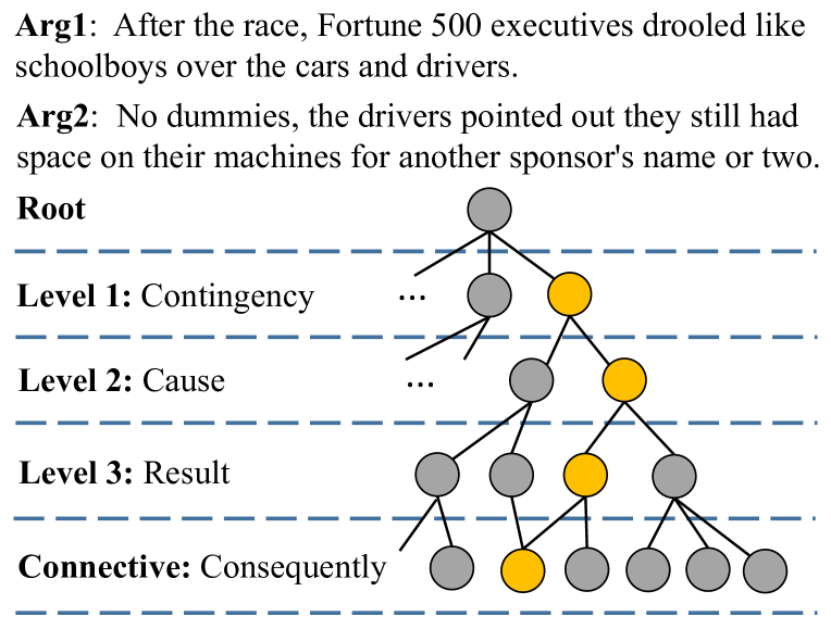
Figure 1: An Instance for multi-level IDRR.

Since pre-trained language models (PLMs) are widely applied, IDRR has also achieved considerable improvement. However, previous work Xu et al. (2018); Shi et al. (2018); Dou et al. (2021) has mentioned the data scarcity of the IDRR, in which data is insufficient to support deep neural networks to depict the high-dimensional task-specific feature space accurately. Simultaneously, the hierarchical division of discourse relations is complex, and the extraction of hierarchical semantics relies on a large scale of data to sustain.

Previous studies Xu et al. (2018); Dai and Huang (2019); Kishimoto et al. (2020); Guo et al. (2020); Shi and Demberg (2021) alleviate this problem by data augmentation or additional knowledge. However, there are several deficiencies: 1) the difficulty of annotating sufficient data and introducing appropriate knowledge is considerable; 2) noisy data drive models to deviate from the target feature distribution, and unreasonable knowledge injection exacerbates the collapse of feature space of PLMs.

Recently, some prompt tuning (PT) methods Hambardzumyan et al. (2021); Li and Liang (2021); Lester et al. (2021); Liu et al. (2021a); Zhang et al. (2022) have shown remarkable results in low resource scenarios (i.e., parameter-efficient prompt tuning, PEPT). They freeze most or all parameters of PLMs and leverage a few additional parameters to restrict the approximation in a small manifold, thus reducing the dependency on the scale of data.

Inspired by the above, we leverage the PEPT to drive the input to match the pre-trained feature space and further present a Parameter-Efficient Multi-level IDRR framework (PEMI), which alleviates the under-training problem caused by data scarcity and infuses hierarchical guidance into the prompt verbalizer. Thus we can mine better context patterns guided by hierarchical label signals for the IDRR. Generally, prompt-based framework mostly consists of two parts: template engineering and verbalizer engineering.

For the template formulation, instead of manually designed templates, we inject soft prompts into the template and regard them as learnable global context vectors to mine the unique pattern of arguments and adjust input features to align the target distribution under the pre-trained semantic space.

However, this alignment is marginal, so it is crucial to adopt the verbalizer for the masked language model (MLM), which maps several label words in vocab to a specific category. But these verbalizer does not have access to learn the hierarchical connection of discourse relations. Besides, existing methods Wu et al. (2020); Chen et al. (2021); Wu et al. (2022); Wang et al. (2022) require feature alignment or extra structure (e.g., GCN, CRF), which conflicts with the hypothesis of PEPT. Therefore, we propose a novel method called hierarchical label refining (HLR) to incorporate hierarchical information into the verbalizer. In our method, only the bottom-level label words are parameterized. Others are refined from the bottom up according to the hierarchical division. And the dispersed label semantics are continuously aggregated to more generalized ones in each iteration, thus realizing the dynamic updating of the verbalizer.

Finally, our framework carries out joint learning at all levels, thus combining the intra-level label discrimination process and the inter-level hierarchical information integration process.

Our contributions are summarized as follows:

• Initially leverage PEPT to drive arguments to match the pre-trained feature space and alleviate the data scarcity of IDRR from the parameter side.

• Propose a parameter-efficient multi-level IDRR framework, deeply infusing hierarchical label guidance into prompt tuning and jointly mining the unique patterns of arguments and labels for MIDRR.

• Results and visualization demonstrate the effectiveness of our framework with only 100K trainable parameters.

2 Related Work

2.1 Implicit discourse relation recognition

We introduce deep learning methods for the IDRR Pitler et al. (2009) through two routes.

One route is argument pair enhancement. The early work (Zhang et al., 2015; Chen et al., 2016; Qin et al., 2016; Bai and Hai, 2018) tends to build a heterogeneous neural network to acquire structured argument representations. Besides, other methods (Liu and Li, 2016; Lan et al., 2017; Guo et al., 2018; Ruan et al., 2020; Liu et al., 2020) focus on capturing interactions between arguments. Moreover, several methods (Dai and Huang, 2018; Kishimoto et al., 2018; Guo et al., 2020; Kishimoto et al., 2020; Zhang et al., 2021) aim at obtaining robust representations based on data augmentation or knowledge projection. However, these methods lack the exploration of relation patterns.

Another route is discourse relation enhancement. These methods are not only concerned with argument pairs but also discourse relations. He et al. (2020) utilizes a triplet loss to establish spatial relationships between arguments and relation representation. Jiang et al. (2021) tends to predict a response related to the target relation. Most studies Nguyen et al. (2019); Wu et al. (2020, 2022) import different levels of relations to complete task understanding. However, they lack consideration of data scarcity and weaken the effectiveness of PLMs. We combine prompt tuning with hierarchical label refining to mine argument and label patterns from a multi-level perspective and adopt a parameter-efficient design to alleviate the above problems.

2.2 Prompt Tuning

The essence of prompt-based learning is to bridge the gap between the MLM and downstream tasks by reformulating specific tasks as cloze questions. At present, there are some papers (Xiang et al., 2022b; Zhou et al., 2022) that make hand-crafted prompts to achieve promotion for IDRR. However, they require numerous experiments to obtain reliable templates.

Recently, prompt tuning (PT) Liu et al. (2022); Ding et al. (2022) is proposed to search for prompt tokens in a soft embedding space. Depending on resource scenarios, it can be mainly divided into two kinds of studies: full prompt tuning (FPT) and parameter-efficient ones (PEPT).

With sufficient data, FPT Han et al. (2021); Liu et al. (2021b); Wu et al. (2022) combines the parameters of PLM with soft prompts to accomplish the bidirectional alignment of semantic feature space and inputs. Among them, P-Tuning Liu et al. (2021b) replaces the discrete prompts with soft ones and adopts MLM for downstream tasks. PTR Han et al. (2021) concatenates multiple sub-templates and selects unique label word sets for different sub-prompts.

However, in the low-resource scenario, this strategy cannot accurately depict the high-dimensional task-specific space. Therefore, PEPT methods Hambardzumyan et al. (2021); Lester et al. (2021); Li and Liang (2021); Liu et al. (2021a); Zhang et al. (2022); Gu et al. (2022) consider fixing the parameters of PLMs, and leverage soft prompts to map the task-specific input into unified pre-trained semantic space. For example, WARP Hambardzumyan et al. (2021) uses adversarial reprogramming to tune input prompts and the self-learning Verbalizer to achieve superior performance on NLU tasks. Prefix-Tuning Li and Liang (2021) tunes PLMs by updating the pre-pended parameters in each transformer layer for NLG. In this paper, we combine PEPT with our proposed hierarchical label refining method, which not only takes full advantage of PEPT for IDRR, but also effectively integrates the extraction of hierarchical guidance into the process of prompt tuning.

3 Overall Framework

Let $\bm{x}=(\bm{x}_{1},\bm{x}_{2})\in\mathcal{X}$ be an argument pair and $\mathbb{L}=\left(L^{1},L^{2},..,L^{\mathcal{Z}}\right)$ be the set of total labels, where $L^{z}$ is the level-$z$ label set. The goal of the MIDRR is to predict the relation sequence $\bm{l}=l^{1},\ldots,l^{z},\ldots,l^{\mathcal{Z}}$, where $l^{z}\in L^{z}$ is the prediction of level $z$. The overview of our framework is shown in Figure 2. In this section, we explain our framework in three parts. First, we analyze the theory of PEPT for single-level IDRR and infer the association with our idea. Next, we describe how to expand the PEPT to MIDRR through our proposed hierarchical label refining method. Finally, we conduct joint learning with multiple levels so as to fuse the label information of inter and intra-levels.

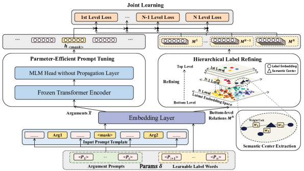
Figure 2: The overall architecture of our PEMI framework.

3.1 Prompt Tuning for Single-level IDRR

Prompt tuning is a universal approach to stimulate the potential of PLMs for most downstream tasks, which goal is to find the best prompts that make the MLM predict the desired answer for the <mask> in templates. It is also suitable for single-level IDRR. Inspired by a PEPT method called WARP Hambardzumyan et al. (2021), we desire to achieve objective approximations with fewer parameters for the data scarcity of IDRR. And to our knowledge, our work is the first successful application of PEPT to the IDRR.

In theory, given a MLM $\mathcal{M}$ and its vocabulary $\mathcal{V}$, it is requisite to transform $z$-th level IDRR into a MLM task. Therefore, for the input $\bm{x}$, we first construct a modified input $\tilde{\bm{x}}\in\tilde{\mathcal{X}}$ through template projection $\mathcal{T}:\mathcal{X}\rightarrow\tilde{\mathcal{X}}$, which surrounds by soft prompts $\mathcal{P}=\{\langle\mathbf{P}_{0}\rangle,\langle\mathbf{P}_{1}\rangle,...,\langle\mathbf{P}_{K-1}\rangle\}\subset\mathcal{V}$ ($K$ represents the number of $\mathcal{P}$) and special tokens <mask> and <sep>. These soft prompt tokens are the same as other words in $\mathcal{V}$. But they do not refer to any real word and are learnable through gradient backpropagation. So the actual input $\tilde{\bm{x}}\in\tilde{\mathcal{X}}$ can be formulated as follows:

$$\begin{split}\tilde{\bm{x}}=&\mathcal{T}(x)\\ =&[\langle\mathbf{P}_{0:k_{1}}\rangle,\bm{x}_{1},\langle\mathbf{P}_{k_{1}+1:k_{2}}\rangle,\langle mask\rangle,\langle sep\rangle\\ &\langle\mathbf{P}_{k_{2}+1:k_{3}}\rangle,\bm{x}_{2},\langle\mathbf{P}_{k_{3}+1:K-1}\rangle]\end{split}$$ (1)

where $\langle\mathbf{P}_{0:k_{1}}\rangle$ indicates the aggregation of $\langle\mathbf{P}_{i}\rangle\in\mathcal{V}$ and $i\in[0,k_{1}]$. The value of $k_{1},k_{2},k_{3}$ is optional, and we will discuss the main factors of template selection in 4.6.

Then, we hope to leverage the MLM $\mathcal{M}$ to predict discourse relations. We denote $\mathcal{E}:\tilde{\mathcal{X}}\rightarrow\mathcal{H}$ and $\mathcal{F}:\mathcal{H}\rightarrow\mathcal{V}$ as the encoder and vocabulary classifier of $\mathcal{M}$. For encoder $\mathcal{E}$, we do not make extra modifications and obtain the feature representation $\mathbf{h}_{\langle mask\rangle}\in\mathcal{H}$ from <mask> position. Through the attention in $\mathcal{E}$, prompts can constantly mine the context pattern and guide to acquire semantic representations with IDRR characteristics. While for $\mathcal{F}$, label word selection should be made to constrain the probabilities to fall on words associated with relation labels. Here, instead of picking up verbalizer through handcraft or rules, we adopt self-learning verbalizer $\mathcal{V}^{z}=\{\langle\bm{V}_{0}\rangle,\langle\bm{V}_{1}\rangle,...,\langle\bm{V}_{|L^{z}|}\rangle\}\subset\mathcal{V}$ to represent label words for level-$z$ classes. We denote this new projection as $\mathcal{F}^{z}:\mathcal{H}\rightarrow\mathcal{V}^{z}$. In practice, we replace the final projection in $\mathcal{F}$ with verbalizer embedding matrix $\mathbf{M}^{z}\in\mathbb{R}^{|L^{z}|\times d}$ to acquire $\mathcal{F}^{z}$. The matrix $\mathbf{M}^{z}$ represents as:

$$\mathbf{M}^{z}=\left[\bm{e}(\langle\bm{V}_{0}\rangle);\bm{e}(\langle\bm{V}_{1}\rangle);\ldots;\bm{e}(\langle\bm{V}_{|L^{z}|}\rangle)\right]$$ (2)

where $\bm{e}(\cdot)$ is the embedding projection of $\mathcal{M}$. And the calculation of $\mathcal{F}^{z}$ is as follows:

$$\mathcal{F}^{z}(\bm{h}_{\langle mask\rangle})=\hat{\mathbf{y}}^{z}=\textrm{softmax}(\mathbf{M}^{z}\mathbf{h}^{{}^{\prime}}_{\langle mask\rangle})$$ (3)

where $\hat{\mathbf{y}}^{z}=\{\hat{y}_{i}^{z}\}^{|L^{z}|}_{i=1}$ is the probabilistic predictions of the $z$-th level and $\mathbf{h}^{{}^{\prime}}_{\langle mask\rangle}$ is the representation before verbalizer projection. There are different operations for each PLM (e.g., layer norm).

Finally, we train this model through cross-entropy loss to approximate the real distribution of $z$-th level as follows:

$$\mathcal{L}^{z}=-\sum_{i=1}^{|L^{z}|}y^{z}_{i}\log(\hat{y}^{z}_{i})$$ (4)

where $\mathbf{y}^{z}=\{y_{i}^{z}\}^{|L^{z}|}_{i=1}$ is the one-hot representation of ground-truth relation.

Although we can narrow the gap between pre-training and IDRR by the above, it is inappropriate to fine-tune the pre-trained feature space to task-specific ones in low-resource scenarios, which will further aggravate the collapse of the vanilla space. Therefore, we propose to approximate the original objective by adjusting the input to fit vanilla PLM space. Let $\theta_{\mathcal{M}}$ be the parameters of $\mathcal{M}$ and $\delta=\{\theta_{P},\theta_{\mathcal{V}^{z}}\}$ represents the parameters of soft prompts and verbalizer. Our method seeks to find a new approximate objective function $\hat{\mathcal{L}}^{z}(\cdot;\delta)$, such that:

$$|\mathcal{L}^{z}(x,y;\theta_{\mathcal{M}},\delta)-\hat{\mathcal{L}}^{z}(x,y;\delta)|<\epsilon$$ (5)

where $\epsilon$ is the approximation error.

Moreover, if we assume that the difference of $\mathcal{F}^{z}$ between $\mathcal{L}^{z}$ and $\hat{\mathcal{L}}^{z}$ is insignificant when $\mathcal{L}^{z}$ reaches its optimal, the purpose of PEPT can be understood as:

$$\mathcal{E}(\mathcal{T}(x;\theta_{\mathcal{P}}))\rightarrow\mathcal{E}^{+}(\mathcal{T}(x;\theta_{\mathcal{P}});\theta_{\mathcal{M}})$$ (6)

where $\mathcal{E}^{+}$ is the optimal encoder. Through this method, we restrict MLM into a small manifold in the functional space Aghajanyan et al. (2021), thus adjusting the input to fit the original PLM feature space. Especially in low-resource situations, this approach can effectively achieve approximation.

3.2 Hierarchical Label Refining

Despite the success of single-level IDRR, PEPT suffers from the absence of hierarchical label guidance. Besides, existed hierarchical infusion method Wu et al. (2020); Chen et al. (2021); Wu et al. (2022); Wang et al. (2022) undoubtedly introduces additional parameters except for $\delta$, which accelerates the deconstruction of pre-trained feature space.

Therefore, we propose a hierarchical label refining (HLR) method that integrates hierarchical guidance on the verbalizer. Not only does our method not increase the scale of $\theta_{\mathcal{V}}=\{\theta_{\mathcal{V}^{m}}\}_{m=1}^{Z}$, but also restrict the parameters to $\theta_{\mathcal{V}^{Z}}$.

In detail, for multi-level IDRR, the arguments are annotated by different semantic granularity in the process of labeling. And all the labels can form a graph $\mathcal{G}$ with $Z$ levels according to the pre-defined relationships. In this graph, for a particular $z$-th level label $l_{j}^{z}$ ($j\in\{1,2,...,|L^{z}|\}$), its relevant sub-labels are distributed in level z+1 and we denote them as:

$$\begin{split}L^{z+1}_{j}=&\{l^{z+1}|Parent\left(l^{z+1}_{t}\right)=l_{j}^{z}\}\\ &where\ t\in\{1,2,\ldots,|L^{z+1}|\}\end{split}$$ (7)

where $Parent(\cdot)$ means the parent node of it.

In abstract, the nodes in $L^{z+1}_{j}$ are the semantic divisions of $l_{j}^{z}$, which represent the local meaning of $l_{j}^{z}$. In other words, the meaning of $l_{j}^{z}$ can be extracted by merging its sub-labels. While in the embedding space, this relationship can be translated into clustering, where $l_{j}^{z}$ represents the semantic center of its support set $L^{z+1}_{j}$. Therefore, if the embeddings for sub-labels make sense, we can regard the semantic center extracted by them as their parent label. Under this concept, we only need to build the semantics of the bottom-level labels, and other levels are produced by aggregation from the bottom up. From the view of the graph neural networks, our method limits the adjacent nodes of each node in $\mathcal{G}$ to be the fine-grained labels of the first-order neighborhood, and the updating of node embeddings only depends on the aggregation of the adjacent nodes without itself. In practice, the verbalizer $\mathcal{V}^{*}$ only consists of $|L^{\mathcal{Z}}|$ learnable label words and others are generated from $\mathcal{V}^{*}$.

Furthermore, we discuss how to achieve effective semantic refining. A major direction is the proportion of support nodes. However, the weights of refining depend on numerous factors, e.g., the label distribution of datasets, the semantic importance of the parent label, polysemy and so on. Hence we apply several learnable weight units in the process of refining to balance the influence of multiple factors, which is equal to adding weights to the edges in $\mathcal{G}$. All the weights are acquired through the iteration of prompt tuning. Formally, the element of the weight vector $\bm{w}_{j}^{z}=\left[w_{j,i}^{z}\right]_{i=1}^{|L^{z+1}|}$ for $l_{j}^{z}$ are obtained as follows:

$$w_{j,i}^{z}=\left\{\begin{array}[]{ll}unit(z,i,j)&l_{i}^{z+1}\in L_{j}^{z+1}\\ 0&otherwise\\ \end{array}\right.$$ (8)

where $unit(*)$ is the function to obtain the target weight unit controlled by $z$, $i$, and $j$.

After that, We formalize the calculation of the verbalizer matrix $\bm{M}^{z}$ at $z$-th level as follows:

$$\mathbf{M}^{z}=\left\{\begin{array}[]{ll}\left[\bm{e}(\langle\bm{V}_{0}\rangle);\ldots;\bm{e}(\langle\bm{V}_{|L^{\mathcal{Z}}|}\rangle)\right]&z=\mathcal{Z}\\ f(\mathbf{W}^{z})\cdot\mathbf{M}^{z+1}&otherwise\end{array}\right.$$ (9)

where $\mathbf{W}^{z}=\left[\mathbf{w}_{1}^{z};\bm{w}_{j}^{z};...;\bm{w}_{|L^{z}|}^{z}\right]$ is the weight matrix of $z$-th level, and $f(\cdot)$ stands for the normalization method like softmax and $L_{1}$ norm.

Our method repeats this process from the bottom up to get semantic embeddings at all levels. And it is performed in each iteration before the calculation of the objective function, thus aggregating upper semantics according to more precise basic ones and infusing it into the whole process of PT. In this way, discourse relations produce hierarchical guidance from the generation process and continue to enrich the verbalizer $\mathcal{V}^{*}$.

3.3 Joint Learning

After the embeddings of all levels are generated vertically, we conduct horizontal training for intra-level senses. Precisely, we first calculate the probability distribution of each level independently. The calculations of each level follow Equation (3) and (4).

Eventually, our model jointly learns the overall loss functions as the weighted sum of Equation (4):

$$\mathcal{L}=\sum_{t=1}^{Z}\lambda_{z}\mathcal{L}^{(z)}$$ (10)

where $\lambda_{z}$ indicates the trade-off hyper-parameters to balance the loss of different levels. By joint learning for different levels, our model naturally combines the information within and between hierarchies. Besides, it can synchronously manage all the levels through one gradient descent, without multiple iterations like the sequence generation model, thus speeding up the calculation while keeping hierarchical label guidance information.

4 Experiments

4.1 Dataset

To facilitate comparison with previous work, we evaluate our model on PDTB 2.0 and 3.0 datasets. The original benchmark Prasad et al. (2008) contains three-level relation hierarchies. However, the third-level relations cannot conduct classification due to the lack of samples in most of the categories. Following previous work (Wu et al., 2020, 2022), we regard the connectives as the third level for MIDRR. The PDTB 2.0 contains 4 (Top Level), 16 (Second Level) and 102 (Connectives) categories for each level. For the second-level labels, five of them without validation and test instances are removed. For PDTB 3.0, following Kim et al. (2020), we conduct 4-way and 14-way classifications for the top and second levels. Since previous work has not defined the criterion for PDTB 3.0 connectives, we choose 150 connectives in implicit instances for classification. For data partitioning, we conduct the most popular dataset splitting strategies PDTB-Ji Ji and Eisenstein (2015), which denotes sections 2-20 as the training set, sections 0-1 as the development set, and sections 21-22 as the test set. More details of the PDTB-Ji splitting are shown in Appendix A.

4.2 Experimental Settings

Our work uses Pytorch and Huggingface libraries for development, and also verifies the effectiveness of our model on MindSpore library. For better comparison with recent models, we apply RoBERTa-base Liu et al. (2019) as our encoder. All of the hyper-parameters settings remain the same as the original settings for it, except for the dropout is set to 0. And we only updates the parameters of $\delta=\{\theta_{\mathcal{P}},\theta_{\mathcal{V}^{\mathcal{Z}}}\}$ and weight units $\{\bm{W}^{z}\}^{\mathcal{Z}}_{z=1}$ while freezing all the other parameters when training. The weight coefficients of loss function $\lambda_{z}$ are 1.0 equally. And the normalized function $f$ is softmax. In order to verify the validity of the results, we choose Adam optimizer and learning rate 1$e$-3 with a batch size of 8. The training strategy conducts early stopping with a maximum of 15 epochs and chooses models based on the best result on the development set. The evaluation step is 500. In practice, one training process of PEMI takes about 1.5 hours on a single RTX 3090 GPU. Finally, We choose the macro-$F_{1}$ and accuracy as our validation metrics.

4.3 The Comparison Models

Model	Embedding Layer	Top Level (4-way)		Second Level (11-way)		Connectives (102-way)		Trainable Params
		$F_{1}$	$Acc$	$F_{1}$	$Acc$	$F_{1}$	$Acc$
FT-RoBERTa Liu et al. (2019)	RoBERTa	61.62	68.57	38.55	58.43	7.89	29.68	>125M
BMGF Liu et al. (2020)	RoBERTa	63.39	69.06	-	58.13	-	-	>15M
MTL-KT Nguyen et al. (2019)	RoBERTa	61.89	68.42	38.10	57.72	7.75	29.57	>125M
MT-BERT Kishimoto et al. (2020)	BERT	58.48	65.26	-	54.32	-	-	>110M
TransS-RoBERTa He et al. (2020)	RoBERTa	61.57	69.28	37.83	57.76	7.83	31.38	>125M
HierMTN-CRF Wu et al. (2020)	BERT	55.72	65.26	33.91	52.34	10.37	30.00	>110M
HierMTN-CRF Wu et al. (2020)	RoBERTa	62.02	70.05	38.28	58.61	10.45	31.30	>125M
CG-T5 Jiang et al. (2021)	T5	57.18	-	37.76	-	-	-	>250M
LDSGM Wu et al. (2022)	RoBERTa	63.73	71.18	40.49	60.33	10.68	32.20	>155M
Ours	RoBERTa	64.05	71.13	41.31	60.66	10.87	35.32	<100K

Table 1: Experimental results for Macro-$F_{1}$ score (%), Accuracy (%) and Trainable Parameters on PDTB 2.0. The results of FT-RoBERTa and TransS-RoBERTa are obtained under our settings.

Second Level	Label-wise F1 (%)
	BMGF	LDSGM	Ours
Comp.Concession	0	0	8.11
Comp.Contrast	59.75	63.52	60.20
Cont.Cause	59.60	64.36	61.82
Cont.Pragmatic cause	0	0	0
Expa.Alternative	60.00	63.46	60.54
Expa.Conjunction	60.17	57.91	50.71
Expa.Instantiation	69.96	72.6	73.81
Expa.List	0	8.98	30.55
Expa.Restatement	53.83	58.06	55.60
Temp.Asynchronous	56.18	56.47	53.04
Temp.Synchrony	0	0	0

Table 2: The second-level label-wise $F_{1}$ on PDTB 2.0. Comp, Cont, Expa and Temp represents Comparison, Contingency, Expansion and Temporal separately.

In this section, we select some baselines for PDTB 2.0 and 3.0 separately and introduce them briefly:
$\bullet\$PDTB 2.0 : We select some comparable models based on PLMs and briefly introduce them through two aspects:
Argument Pair Enhancement

1) FT-RoBERTa: Liu et al. (2019) improves the BERT by removing the NSP task and pre-training on wide corpora. We conduct experiments for each level separately.

2) BMGF: Liu et al. (2020) proposes a bilateral multi-perspective matching encoder to enhance the arguments interaction on both text span and sentence level.
Discourse Relation Enhancement

3) MTL-KT: Nguyen et al. (2019) predicts relations and connectives simultaneously and transfers knowledge via relations and connectives through label embeddings. We import the RoBERTa version from Wu et al. (2022).

4) MT-BERT: Kishimoto et al. (2020) proposes a multi-task learning model which additionally predicts connectives and explicit discourse relations and adds extra data.

5) TransS-RoBERTa: He et al. (2020) uses triplet loss to introduce geometric structure into semantic representation space. We replace the embedding layer with RoBERTa for a fair comparison.

6) HierMTN-CRF: Wu et al. (2020) firstly deals with multi-level IDRR simultaneously and chooses the label sequence based on a CRF layer. We import its BERT and RoBERTa versions.

7) CG-T5: Jiang et al. (2021) combines the IDRR classification with generation by generating adequate sentences related to discourse relations with several templates.

8) LDSGM: Wu et al. (2022) views IDRR as a label sequence prediction task and leverages the label dependencies between discourse relations through GCN and conducts label sequence prediction by a GRU decoder.
$\bullet\$PDTB 3.0 :

1) NNMA: Liu and Li (2016) imitates repeat reading habit by applying stacked attention mechanisms on the representations of argument pair.

2) MANN: Lan et al. (2017) regards the IDRR for multiple datasets as multi-task learning and applies interactive attention based on BiLSTM.

3) IPAL: Ruan et al. (2020) divides argument pair encoding into two channels and combines self-attention and interactive attention by a cross-coupled network.

4) MANF: Xiang et al. (2022a) proposes dual attention and encodes word-pairs offsets to enhance semantic interaction. We import the word2vec and BERT versions of it.

5) FT-RoBERTa: we also fine-tune a RoBERTa model on PDTB 3.0 for better comparison.

4.4 Results and Analysis

Model	Macro-F1
	Top	Second	Conn
Baseline	61.29	39.19	8.12
+PEPT	63.16	40.71	9.89
+HLR	62.85	40.82	8.94
+PEPT&HLR (Ours)	64.05	41.31	10.87

Table 3: Ablation study on PDTB 2.0. Our Baseline choose fine-tuned RoBERTa MLM with a learnable verbalizer. PEPT means parameter-efficient prompt tuning and HLR is the hierarchical label refining.

In this section, we display the main results of three levels on PDTB 2.0 (Table 1) and PDTB 3.0 (Table 7) and the label-wise $F_{1}$ of level 2 on PDTB 2.0 (Table 2) and PDTB 3.0 (Table 6).

We can obtain the following observations from these results: 1) In table 1, our model achieves comparable performance with strong baselines and only uses 0.1% trainable parameters. And the improvement mainly occurs at the level-3 senses, which states that our model is more aware of fine-grained hierarchical semantics. 2) In table 7, compared with baselines, our model exceeds all fine-tuned models currently, which proves that the effect of our model is also guaranteed with sufficient data. 3) In Table 2, our model mainly outperforms on the minor classes. For PDTB 2.0, the improvement depends on three minor categories: Comp.Concession, Expa.List and Expa.Instantiation, which indicates that the approximation through fewer trainable parameters drives the model to pay more attention to minors. More details for PDTB 3.0 are shown in Appendix B.

4.5 Ablation Study and Analysis

We conduct the ablation study on PDTB 2.0 to deeply analyze the impact of our framework. Our Baseline chooses fine-tuned RoBERTa MLM with a learnable verbalizer. Compared with fine-tuned RoBERTa, our baseline acquires arguments representation through <mask> and retains some parameters of MLM head. Besides, it treats IDRR of different levels as an individual classification but shares the parameters of the encoder. And then, we decompose our model into two parts described in Section 3: Parameter-Efficient Prompt Tuning (PEPT) and hierarchical label refining (HLR).

From Table 3, we can observe that: 1) The results of our baseline are higher than the vanilla PLM, which indicates that adapting MLM to the IDRR is more practicable. 2) Baseline+HLR gains improvements on all levels, especially on level 2, which presumes that information from both the upper and lower level labels guides to make it more semantically authentic. 3) PEMI achieves the best performance over other combinations, which proves that PEPT makes HLR not be affected by redundant parameters and focuses on the semantic information in the verbalizer.

4.6 Template Selection

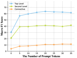
Figure 3: The effect of prompt token size for MIDRR on PDTB 2.0. We follow the best template in Table 8 and try to put them uniformly in each location.

Furthermore, we design experiments on PDTB 2.0 for two main factors of the prompt templates: the location and the size of prompt tokens, as shown in Table 8 and Figure 3 separately.

Table 8 shows that the locations have a great influence on our model. Generally, we note that most of the templates that prompt tokens are scattered surpass the compact ones. So it is beneficial to place scattered around sentences. Meticulous, placing more prompt tokens around the first sentence achieves particular promotion, suggesting that early intervention for prompts could better guide the predictions of discourse relations.

In Figure 3, as the number of prompt tokens increases, the situations are different for three levels. For the level-1 and level-2 senses, they reach the peak when the number rises to 20 and then starts to go down, which indicates that over many prompt tokens may dilute the attention between arguments. However, the performance of connectives continues to improve as the number increases. This is mainly because the difficulty of classification rises and more prompts need to be involved. Therefore, we ultimately measured the performance of all levels and chose 20 prompt tokens as our final result, but there is still room for improvement.

4.7 Impact of Hierarchical Label Refining

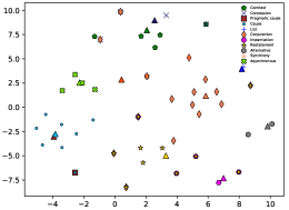
Figure 4: Visualization of HLR method for connectives. $\Delta$ represents level 2 labels and different colors indicate different classes. We use different markers since some connectives are overlapping due to the many-to-many mapping between level 2 and connectives.

Finally, we carry out two experiments to explore the impact of our HLR method: weight coefficients learned by weight units in Table 9 and 10 and visualization of label embeddings in Figure 4.

In Table 9, we find out that most of the weight coefficients are inversely proportional to data size, while a few cases like Expa.Alternative are ignored. Combined with Table 4, we can infer that our model pays more attention to the minor classes and lowers the weight to the good-performing classes.

Besides, in Figure 4, we note that visibly clustering relationships exist in the embedding space. Meanwhile, for the major classes like Cont.Cause and Expa.Conjunction, the class centers tend to be the average of connectives in the cluster. In contrast, minor classes like Expa.Alternative and Expa.List are biased towards a particular connective. The reason is that some connectives belonging to multiple discourse relations can transfer knowledge from other relations and improve the prediction of the current relation. Then the model will increase the weight of those connectives to get closer to the actual distribution. Therefore, it can be said that the HLR method transfers the inter and intra-level guidance information in the embedding space.

5 Conclusion

In this paper, we tackle the problem of data scarcity for IDRR from a parameter perspective and have presented a novel parameter-efficient multi-level IDRR framework, which leverages PEPT to adjust the input to match the pre-trained space with fewer parameters and infuse hierarchical label guidance into the verbalizer. Experiments show that our model adopts parameter-efficient methods while it is comparable with recent SOTA models. Besides, it indicates that our framework can effectively stimulate the potential of PLMs without any intervention of additional data or knowledge. In the future, we will further explore the linguistic features of labels and enhance the discrimination against connectives.

Limitations

Although our model obtains satisfying results, it also exposes some limitations. First, for a fair comparison to other models, we mainly carry out relevant experiments on PDTB 2.0. Due to the lack of baselines on PDTB 3.0, further analysis and comparison cannot be conducted. Second, in our experiments, we can find out that the HLR method does not improve the top-level or bottom-level results effectively, indicating that with the increase of the level, the refining method is insufficient to continue to generalize the bottom-level labels and further improvement should be made according to the specific features of the IDRR task. Third, due to the limitation of space, this paper does not focus much on semantic weight for the refining of sub-labels. This is a very broad topic involving the rationality of the discourse relation annotation and the interpretability of the label embeddings. We will conduct a further study which may appear in our next work.

Appendices

Appendix A Details of PDTB-Ji Splitting

In this section, we provide data statistics of level 2 for PDTB 2.0 (Table 4) and PDTB 3.0 (Table 5) separately.

Second Level	Sample Size
	Train	Dev	Test
Comp.Concession	183	15	17
Comp.Contrast	1607	166	128
Cont.Cause	3270	281	269
Cont.Pragmatic cause	64	6	7
Expa.Alternative	147	10	9
Expa.Conjuction	2872	258	200
Expa.Instantiation	1063	106	118
Expa.List	338	9	12
Expa.Restatement	2404	260	211
Temp.Asynchronous	532	46	54
Temp.Synchronous	203	8	14
Total	12683	1165	1039

Table 4: Statistics for relation senses of Level 2 in PDTB 2.0 by PDTB-Ji splitting.

Second Level	Sample Size
	Train	Dev	Test
Comp.Concession	1164	103	97
Comp.Contrast	741	82	54
Cont.Cause	4475	448	404
Cont.Cause+Belief	159	13	15
Cont.Condition	150	18	15
Cont.Purpose	1092	96	89
Expa.Conjuction	3586	298	236
Expa.Equivalence	254	25	30
Expa.Instantiation	1166	116	124
Expa.Level-of-detail	2601	261	208
Expa.Manner	615	14	17
Expa.Substitution	343	27	26
Temp.Asynchronous	1007	101	105
Temp.Synchronous	435	33	43
Total	17788	1635	1463

Table 5: Statistics for relation senses of Level 2 in PDTB 3.0 by PDTB-Ji splitting.

Appendix B Experimental Results on PDTB 3.0

Due to the limitation of pages, we provide results of PDTB 3.0 in this section. Table 6 displays the label-wise F1 for level-2 senses on PDTB 3.0 and Table 7 shows the main results on PDTB 3.0 compared with the baselines we stated in Section 4.3.

Second Level	Label-wise F1(%)
	PEMI (Ours)
Comp.Concession	64.68
Comp.Contrast	52.94
Cont.Cause	69.04
Cont.Cause+Belief	0.00
Cont.Condition	68.97
Cont.Purpose	91.49
Expa.Conjuction	58.82
Expa.Equivalence	0.00
Expa.Instantiation	70.42
Expa.Level-of-detail	54.25
Expa.Manner	59.26
Expa.Substitution	48.98
Temp.Asynchronous	66.67
Temp.Synchronous	32.73

Table 6: The second-level label-wise F1 on PDTB 3.0.

Model	Embedding Layer	Top-level (4-way)		Second-level (14-way)		Connective (150-way)		Trainable Params
		$F_{1}$	$Acc$	$F_{1}$	$Acc$	$F_{1}$	$Acc$
NNMA Liu and Li (2016)	GloVe	46.13	57.67	-	-	-	-	>5M
MANN Lan et al. (2017)	word2vec	47.29	57.06	-	-	-	-	>1M
IPAL Ruan et al. (2020)	BERT	49.45	58.01	-	-	-	-	>110M
MANF Xiang et al. (2022a)	word2vec	53.14	60.45	-	-	-	-	>10M
MANF Xiang et al. (2022a)	BERT	56.63	64.04	-	-	-	-	>110M
FT-RoBERTa Liu et al. (2019)	RoBERTa	66.94	71.91	51.78	61.24	10.07	40.26	>125M
Ours	RoBERTa	69.06	73.27	52.73	63.09	10.52	39.92	<130K

Table 7: Experimental results for Macro-$F_{1}$ score (%), Accuracy (%) and Trainable Parameters on PDTB 3.0. The results of FT-RoBERTa are conducted based on our experimental settings.

Appendix C Selection of Input Templates

In this section, we provide several templates by changing the location of prompt tokens and $\langle mask\rangle$ to explore the validity of IDRR. And Table 8 shows the overall results for reference. Finally, we find out that it is preferable to put the $\langle mask\rangle$ token in the middle of the argument pair, as described in Section 3.1.

Template Form	Top-level		Second-level		Connective
	$F_{1}$	$Acc$	$F_{1}$	$Acc$	$F_{1}$	$Acc$
$\langle\textrm{P:4}\rangle\bm{S_{1}}\langle\textrm{P:4}\rangle\langle\textrm{mask}\rangle\langle\textrm{P:4}\rangle\langle\textrm{sep}\rangle\langle\textrm{P:4}\rangle\bm{S_{2}}\langle\textrm{P:4}\rangle$	64.05	71.13	41.31	60.66	10.87	35.32
$\langle\textrm{P:5}\rangle\bm{S_{1}}\langle\textrm{P:5}\rangle\langle\textrm{mask}\rangle\langle\textrm{sep}\rangle\langle\textrm{P:5}\rangle\bm{S_{2}}\langle\textrm{P:5}\rangle$	62.73	68.96	41.10	58.98	10.52	34.69
$\langle\textrm{P:5}\rangle\langle\textrm{mask}\rangle\bm{S_{1}}\langle\textrm{P:5}\rangle\langle\textrm{sep}\rangle\langle\textrm{P:5}\rangle\bm{S_{2}}\langle\textrm{P:5}\rangle$	59.71	67.21	37.48	55.62	8.98	33.08
$\langle\textrm{P:5}\rangle\bm{S_{1}}\langle\textrm{P:5}\rangle\langle\textrm{sep}\rangle\langle\textrm{P:5}\rangle\bm{S_{2}}\langle\textrm{mask}\rangle\langle\textrm{P:5}\rangle$	60.54	68.33	37.37	56.72	9.07	34.15
$\langle\textrm{P:20}\rangle\bm{S_{1}}\langle\textrm{mask}\rangle\langle\textrm{sep}\rangle\bm{S_{2}}$	63.62	71.68	38.59	59.44	10.57	35.37
$\langle\textrm{P:20}\rangle\bm{S_{1}}\langle\textrm{sep}\rangle\bm{S_{2}}\langle\textrm{mask}\rangle$	58.66	67.95	37.73	56.67	8.61	33.33
$\langle\textrm{P:20}\rangle\langle\textrm{mask}\rangle\bm{S_{1}}\langle\textrm{sep}\rangle\bm{S_{2}}$	59.32	68.76	38.59	57.91	7.91	32.28
$\bm{S_{1}}\langle\textrm{mask}\rangle\langle\textrm{sep}\rangle\bm{S_{2}}\langle\textrm{P:20}\rangle$	61.91	69.32	40.30	57.80	9.88	35.12
$\langle\textrm{mask}\rangle\bm{S_{1}}\langle\textrm{sep}\rangle\bm{S_{2}}\langle\textrm{P:20}\rangle$	50.38	62.79	35.20	51.80	5.52	27.67
$\bm{S_{1}}\langle\textrm{sep}\rangle\bm{S_{2}}\langle\textrm{mask}\rangle\langle\textrm{P:20}\rangle$	55.46	63.98	37.99	53.54	6.58	28.45
$\langle\textrm{P:10}\rangle\bm{S_{1}}\langle\textrm{mask}\rangle\langle\textrm{sep}\rangle\bm{S_{2}}\langle\textrm{P:10}\rangle$	62.37	69.09	39.47	57.00	9.31	34.87
$\bm{S_{1}}\langle\textrm{P:10}\rangle\langle\textrm{mask}\rangle\langle\textrm{sep}\rangle\langle\textrm{P:10}\rangle\bm{S_{2}}$	59.43	67.89	38.47	56.00	8.14	34.23
$\langle\textrm{P:10}\rangle\langle\textrm{mask}\rangle\bm{S_{1}}\langle\textrm{sep}\rangle\bm{S_{2}}\langle\textrm{P:10}\rangle$	59.60	68.11	37.57	58.22	8.55	32.73
$\langle\textrm{P:10}\rangle\bm{S_{1}}\langle\textrm{sep}\rangle\bm{S_{2}}\langle\textrm{mask}\rangle\langle\textrm{P:10}\rangle$	60.23	68.07	37.88	58.42	8.71	32.69
$\langle\textrm{P:5}\rangle\bm{S_{1}}\langle\textrm{mask}\rangle\langle\textrm{sep}\rangle\bm{S_{2}}\langle\textrm{P:15}\rangle$	63.36	69.10	36.81	58.71	9.04	37.31
$\langle\textrm{P:5}\rangle\langle\textrm{mask}\rangle\bm{S_{1}}\langle\textrm{sep}\rangle\bm{S_{2}}\langle\textrm{P:15}\rangle$	60.32	68.21	37.50	57.95	9.07	35.11
$\langle\textrm{P:5}\rangle\bm{S_{1}}\langle\textrm{sep}\rangle\bm{S_{2}}\langle\textrm{mask}\rangle\langle\textrm{P:15}\rangle$	60.89	67.08	31.61	51.97	8.62	28.73
$\langle\textrm{P:15}\rangle\bm{S_{1}}\langle\textrm{mask}\rangle\langle\textrm{sep}\rangle\bm{S_{2}}\langle\textrm{P:5}\rangle$	63.03	69.86	39.88	59.74	10.73	35.89
$\langle\textrm{P:15}\rangle\langle\textrm{mask}\rangle\bm{S_{1}}\langle\textrm{sep}\rangle\bm{S_{2}}\langle\textrm{P:5}\rangle$	60.77	68.51	38.07	58.41	9.57	37.11
$\langle\textrm{P:15}\rangle\bm{S_{1}}\langle\textrm{sep}\rangle\bm{S_{2}}\langle\textrm{mask}\rangle\langle\textrm{P:5}\rangle$	61.72	69.55	38.93	59.28	9.49	33.09

Table 8: Results by changing the locations of prompt tokens and $\langle mask\rangle$ on PDTB 2.0. We fix the size of the prompt tokens as 20 and test some of extreme cases based on simple permutations. $\langle\textrm{P:x}\rangle$ represents that there are x prompt tokens inserted on this location.

Appendix D Details of Weignt Units

In this section, we display weight coefficients learned by weight units in section 3.2, as shown in Table 9 and 10. We can observe some characteristics of the weights learned by the units. Comparing Table 4 and 9, it is apparent that the weight is inversely proportional to the number of samples, which suggests that our model intentionally learns features from minor classes. While for the second level, the situation is complicated. Some minor connectives like "meanwhile" in Expa.List are put high weight and others like "furthermore" are quite the opposite. Therefore, is not enough to learn a good weight from sample size. Besides, since connectives can belong to different labels, the semantics learned from other relations can be beneficial for the current ones.

Label	Sub Label (Weight (%))
Comp	Contrast (51.83), Concession (48.17)
Cont	Pragmatic cause (70.35), Cause (29.65)
Expa	Alternative (0.66), Conjunction (46.07),  Instantiation (6.67), List (45.60),  Restatement (1.01)
Temp	Synchrony (60.16), Asynchronous (39.84)

Table 9: Weights between top and second levels.

Label	Sub Label (Weight (%))
Concession	while(4.91), however(3.55),  but(3.66), even though(12.28),  nevertheless(7.17), still(5.41),  nonetheless(31.82), yet(4.65),  in fact(4.60), although(3.61),  by comparison(18.35)
Pragmatic  cause	because(0.77), as(0.84),  in fact(1.24), since(2.10),  inasmuch as(86.28), so(1.99)  for example(1.06), thus(2.19),  for instance(1.09), indeed(2.45)
List	and(11.28), first(9.24),  while(4.89), second(2.99),  finally(13.82), in addition(4.83),  also(3.39), meanwhile(17.53),  third(2.54), furthermore(2.80),  for instance(3.09), in fact(5.05),  although(18.56)
Instantiation	indeed(4.37), for instance(9.94),  first(4.29), specifically(4.78),  in fact(4.63), for example(6.64),  for one thing(16.44), and(5.75),  for one(3.01), in particular(3.85),  on one hand(18.69), as(17.61)
Synchrony	meanwhile(6.61), while(6.40),  at the time(7.43), when(9.18),  as(5.49), at that time(3.86),  then(4.13), and(13.22),  simultaneously(16.46),  in the meantime(13.07),  at the same time(14.14)

Table 10: Partial weights between second-level and connectives.

References

- Aghajanyan et al. (2021) Armen Aghajanyan, Luke Zettlemoyer, and Sonal Gupta. 2021. Intrinsic dimensionality explains the effectiveness of language model fine-tuning. ACL.
- Bai and Hai (2018) Hongxiao Bai and Zhao Hai. 2018. Deep enhanced representation for implicit discourse relation recognition. COLING.
- Chen et al. (2021) Haibin Chen, Qianli Ma, Zhenxi Lin, and Jiangyue Yan. 2021. Hierarchy-aware label semantics matching network for hierarchical text classification. ACL.
- Chen et al. (2016) Jifan Chen, Qi Zhang, Pengfei Liu, Xipeng Qiu, and Xuanjing Huang. 2016. Implicit discourse relation detection via a deep architecture with gated relevance network. ACL.
- Cui et al. (2019) Yin Cui, Menglin Jia, Tsung-Yi Lin, Yang Song, and Serge J. Belongie. 2019. Class-balanced loss based on effective number of samples. CVPR.
- Dai and Huang (2018) Zeyu Dai and Ruihong Huang. 2018. Improving implicit discourse relation classification by modeling inter-dependencies of discourse units in a paragraph. NAACL.
- Dai and Huang (2019) Zeyu Dai and Ruihong Huang. 2019. A regularization approach for incorporating event knowledge and coreference relations into neural discourse parsing. EMNLP (Short).
- Ding et al. (2022) Ning Ding, Yujia Qin, Guang Yang, Fu Wei, Zonghan Yang, Yusheng Su, Shengding Hu, Yulin Chen, Chi-Min Chan, Weize Chen, Jing Yi, Weilin Zhao, Xiaozhi Wang, Zhiyuan Liu, Haitao Zheng, Jianfei Chen, Yang Liu, Jie Tang, Juan Li, and Maosong Sun. 2022. Delta tuning: A comprehensive study of parameter efficient methods for pre-trained language models. ArXiv.
- Dou et al. (2021) Zujun Dou, Yu Hong, Yu Sun, and Guodong Zhou. 2021. Cvae-based re-anchoring for implicit discourse relation classification. EMNLP Findings.
- Feng et al. (2021) Xiachong Feng, Xiaocheng Feng, Bing Qin, and Xinwei Geng. 2021. Dialogue discourse-aware graph model and data augmentation for meeting summarization. IJCAI.
- Gu et al. (2022) Yuxian Gu, Xu Han, Zhiyuan Liu, and Minlie Huang. 2022. Ppt: Pre-trained prompt tuning for few-shot learning. ACL.
- Guo et al. (2020) Fengyu Guo, Ruifang He, J. Dang, and Jian Wang. 2020. Working memory-driven neural networks with a novel knowledge enhancement paradigm for implicit discourse relation recognition. AAAI.
- Guo et al. (2018) Fengyu Guo, Ruifang He, Di Jin, J. Dang, Longbiao Wang, and Xiangang Li. 2018. Implicit discourse relation recognition using neural tensor network with interactive attention and sparse learning. COLING.
- Hambardzumyan et al. (2021) Karen Hambardzumyan, H. Khachatrian, and Jonathan May. 2021. Warp: Word-level adversarial reprogramming. ACL.
- Han et al. (2021) Xu Han, Weilin Zhao, Ning Ding, Zhiyuan Liu, and Maosong Sun. 2021. Ptr: Prompt tuning with rules for text classification. ArXiv.
- He et al. (2020) Ruifang He, Jian Wang, Fengyu Guo, and Yugui Han. 2020. Transs-driven joint learning architecture for implicit discourse relation recognition. ACL.
- Ji and Eisenstein (2015) Yangfeng Ji and Jacob Eisenstein. 2015. One vector is not enough: Entity-augmented distributed semantics for discourse relations. TACL.
- Jiang et al. (2021) Feng Jiang, Yaxin Fan, Xiaomin Chu, Peifeng Li, and Qiaoming Zhu. 2021. Not just classification: Recognizing implicit discourse relation on joint modeling of classification and generation. EMNLP.
- Kim et al. (2020) Najoung Kim, Song Feng, R. Chulaka Gunasekara, and L. Lastras. 2020. Implicit discourse relation classification: We need to talk about evaluation. ACL.
- Kishimoto et al. (2018) Yudai Kishimoto, Yugo Murawaki, and S. Kurohashi. 2018. A knowledge-augmented neural network model for implicit discourse relation classification. COLING.
- Kishimoto et al. (2020) Yudai Kishimoto, Yugo Murawaki, and S. Kurohashi. 2020. Adapting bert to implicit discourse relation classification with a focus on discourse connectives. LREC.
- Lan et al. (2017) Man Lan, Jianxiang Wang, Yuanbin Wu, Zheng-Yu Niu, and Haifeng Wang. 2017. Multi-task attention-based neural networks for implicit discourse relationship representation and identification. EMNLP.
- Lester et al. (2021) Brian Lester, Rami Al-Rfou, and Noah Constant. 2021. The power of scale for parameter-efficient prompt tuning. EMNLP.
- Li and Liang (2021) Xiang Lisa Li and Percy Liang. 2021. Prefix-tuning: Optimizing continuous prompts for generation. ACL.
- Li et al. (2020a) Xiaoya Li, Xiaofei Sun, Yuxian Meng, Junjun Liang, Fei Wu, and Jiwei Li. 2020a. Dice loss for data-imbalanced nlp tasks. ACL.
- Li et al. (2020b) Zhenwen Li, Wenhao Wu, and Sujian Li. 2020b. Composing elementary discourse units in abstractive summarization. ACL.
- Liu et al. (2022) Pengfei Liu, Weizhe Yuan, Jinlan Fu, Zhengbao Jiang, Hiroaki Hayashi, and Graham Neubig. 2022. Pre-train, prompt, and predict: A systematic survey of prompting methods in natural language processing. ACM Computing Surveys (CSUR).
- Liu et al. (2021a) Xiao Liu, Kaixuan Ji, Yicheng Fu, Zhengxiao Du, Zhilin Yang, and Jie Tang. 2021a. P-tuning v2: Prompt tuning can be comparable to fine-tuning universally across scales and tasks. ArXiv.
- Liu et al. (2021b) Xiao Liu, Yanan Zheng, Zhengxiao Du, Ming Ding, Yujie Qian, Zhilin Yang, and Jie Tang. 2021b. Gpt understands, too. ArXiv.
- Liu et al. (2020) Xin Liu, Jiefu Ou, Yangqiu Song, and Xin Jiang. 2020. On the importance of word and sentence representation learning in implicit discourse relation classification. IJCAI.
- Liu and Li (2016) Yang Liu and Sujian Li. 2016. Recognizing implicit discourse relations via repeated reading: Neural networks with multi-level attention. EMNLP.
- Liu et al. (2019) Yinhan Liu, Myle Ott, Naman Goyal, Jingfei Du, Mandar Joshi, Danqi Chen, Omer Levy, M. Lewis, Luke Zettlemoyer, and Veselin Stoyanov. 2019. Roberta: A robustly optimized bert pretraining approach. Facebook AI.
- Nguyen et al. (2019) L. T. Nguyen, Ngo Van Linh, Khoat Than, and Thien Huu Nguyen. 2019. Employing the correspondence of relations and connectives to identify implicit discourse relations via label embeddings. ACL.
- Pitler et al. (2009) Emily Pitler, Annie Louis, and A. Nenkova. 2009. Automatic sense prediction for implicit discourse relations in text. ACL.
- Prasad et al. (2008) R. Prasad, N. Dinesh, Alan Lee, Eleni Miltsakaki, L. Robaldo, A. Joshi, and B. Webber. 2008. The penn discourse treebank 2.0. LREC.
- Qin et al. (2016) Lianhui Qin, Zhisong Zhang, and Zhao Hai. 2016. A stacking gated neural architecture for implicit discourse relation classification. EMNLP.
- Ruan et al. (2020) Huibin Ruan, Yu Hong, Yang Xu, Zhen Huang, Guodong Zhou, and Min Zhang. 2020. Interactively-propagative attention learning for implicit discourse relation recognition. COLING.
- Shi and Demberg (2021) Wei Shi and V. Demberg. 2021. Entity enhancement for implicit discourse relation classification in the biomedical domain. ACL.
- Shi et al. (2018) Wei Shi, Frances Yung, and V. Demberg. 2018. Acquiring annotated data with cross-lingual explicitation for implicit discourse relation classification. DISRPT.
- Subramanian et al. (2021) Shivashankar Subramanian, Afshin Rahimi, Timothy Baldwin, Trevor Cohn, and Lea Frermann. 2021. Fairness-aware class imbalanced learning. EMNLP.
- Tang et al. (2021) Jialong Tang, Hongyu Lin, M. Liao, Yaojie Lu, Xianpei Han, Le Sun, Weijian Xie, and Jin Xu. 2021. From discourse to narrative: Knowledge projection for event relation extraction. ACL.
- Wang et al. (2022) Zihan Wang, Peiyi Wang, Lianzhe Huang, Xin Sun, and Houfeng Wang. 2022. Incorporating hierarchy into text encoder: a contrastive learning approach for hierarchical text classification. ACL.
- Wu et al. (2022) Changxing Wu, Liuwen Cao, Yubin Ge, Yang Liu, Min Zhang, and Jinsong Su. 2022. A label dependence-aware sequence generation model for multi-level implicit discourse relation recognition. AAAI.
- Wu et al. (2020) Changxing Wu, Chaowen Hu, Ruochen Li, Hongyu Lin, and Jinsong Su. 2020. Hierarchical multi-task learning with crf for implicit discourse relation recognition. Knowledge Base System.
- Xiang et al. (2022a) Wei Xiang, Bang Wang, Lu Dai, and Yijun Mo. 2022a. Encoding and fusing semantic connection and linguistic evidence for implicit discourse relation recognition. ACL Findings.
- Xiang et al. (2022b) Wei Xiang, Zhenglin Wang, Lu Dai, and Bang Wang. 2022b. Connprompt: Connective-cloze prompt learning for implicit discourse relation recognition. COLING.
- Xu et al. (2018) Yang Xu, Yu Hong, Huibin Ruan, Jianmin Yao, Min Zhang, and Guodong Zhou. 2018. Using active learning to expand training data for implicit discourse relation recognition. EMNLP.
- Zhang et al. (2015) Biao Zhang, Jinsong Su, Deyi Xiong, Yaojie Lu, Hong Duan, and Junfeng Yao. 2015. Shallow convolutional neural network for implicit discourse relation recognition. EMNLP.
- Zhang et al. (2022) Ningyu Zhang, Luoqiu Li, Xiang Chen, Shumin Deng, Zhen Bi, Chuanqi Tan, Fei Huang, and Huajun Chen. 2022. Differentiable prompt makes pre-trained language models better few-shot learners. NeurIPS, abs/2108.13161.
- Zhang et al. (2021) Yingxue Zhang, Fandong Meng, Peng Li, Ping Jian, and Jie Zhou. 2021. Context tracking network: Graph-based context modeling for implicit discourse relation recognition. NAACL.
- Zhou et al. (2022) Hao Zhou, Man Lan, Yuanbin Wu, YueFeng Chen, and Meirong Ma. 2022. Prompt-based connective prediction method for fine-grained implicit discourse relation recognition. EMNLP Findings, abs/2210.07032.