Enhancing One-Shot Federated Learning Through Data and Ensemble Co-Boosting
Abstract
One-shot Federated Learning (OFL) has become a promising learning paradigm, enabling the training of a global server model via a single communication round. In OFL, the server model is aggregated by distilling knowledge from all client models (the ensemble), which are also responsible for synthesizing samples for distillation. In this regard, advanced works show that the performance of the server model is intrinsically related to the quality of the synthesized data and the ensemble model. To promote OFL, we introduce a novel framework, Co-Boosting, in which synthesized data and the ensemble model mutually enhance each other progressively. Specifically, Co-Boosting leverages the current ensemble model to synthesize higher-quality samples in an adversarial manner. These hard samples are then employed to promote the quality of the ensemble model by adjusting the ensembling weights for each client model. Consequently, Co-Boosting periodically achieves high-quality data and ensemble models. Extensive experiments demonstrate that Co-Boosting can substantially outperform existing baselines under various settings. Moreover, Co-Boosting eliminates the need for adjustments to the client’s local training, requires no additional data or model transmission, and allows client models to have heterogeneous architectures.
1 Introduction
Federated learning (FL) (McMahan et al., 2017) has emerged as a prominent distributed machine learning framework to train a global server model via collaboration among users without sharing their dataset. Though the multi-round parameter-server communication paradigm offers the benefit of effectively exchanging information among clients and the central server, it might not be feasible in the real world. This paradigm brings forth significant challenges: 1) heavy communication burden and the risk of connection drop errors between clients and the server (Li et al., 2020a; Kairouz et al., 2021; Dai et al., 2022), and 2) potential risk for man-in-the-middle attacks (Wang et al., 2021) and various other privacy or security concerns (Mothukuri et al., 2021; Yin et al., 2021).
One-shot FL (OFL) (Guha et al., 2019) has emerged as a solution to these issues by restricting communication rounds to a single iteration, thereby mitigating errors arising from multi-round communication and concurrently diminishing the vulnerability to malicious interception. Furthermore, OFL is more practical, particularly within contemporary model market scenarios (Vartak et al., 2016) where clients predominantly offer pre-trained models. In OFL, the server model is aggregated by distilling knowledge from all client models, commonly using the ensemble, while the ensemble is also responsible for synthesizing data samples for knowledge distillation. Consequently, as illustrated in Guha et al. (2019) and Zhang et al. (2022a), the server model’s performance is intricately linked to both the quality of synthesized data and the ensemble. Thus, the primary challenge in improving performance lies in the process of improving the data and the ensemble.
Existing approaches tend to tackle this challenge by exclusively concentrating on either enhancing the quality of the ensemble or improving the quality of synthetic data. For instance, to bolster ensemble, prior works including Dennis et al. (2021), Heinbaugh et al. (2023), and Diao et al. (2023) modify the local training phase and require additional transmissions. In terms of improving synthetic data, Li et al. (2021) utilizes auxiliary public datasets, Zhou et al. (2020) proposes transmitting distilled datasets to the server, Yang et al. (2023) proposes to use auxiliary diffusion model and Zhang et al. (2022a) employs data-free data generation methods to synthesize data directly from averaged ensemble models. While the distilled server may improve through the above methods, it is noteworthy that these approaches typically follow a sequential process, which means the enhancement of data or the ensemble is a prerequisite step before the server model can benefit, omitting the crucial relationship between them. What’s more, in contemporary model market scenarios where only well-pre-trained models with diverse architectural possibilities are accessible, any modifications to local training or additional data or model transmissions are discouraged and often disallowed.
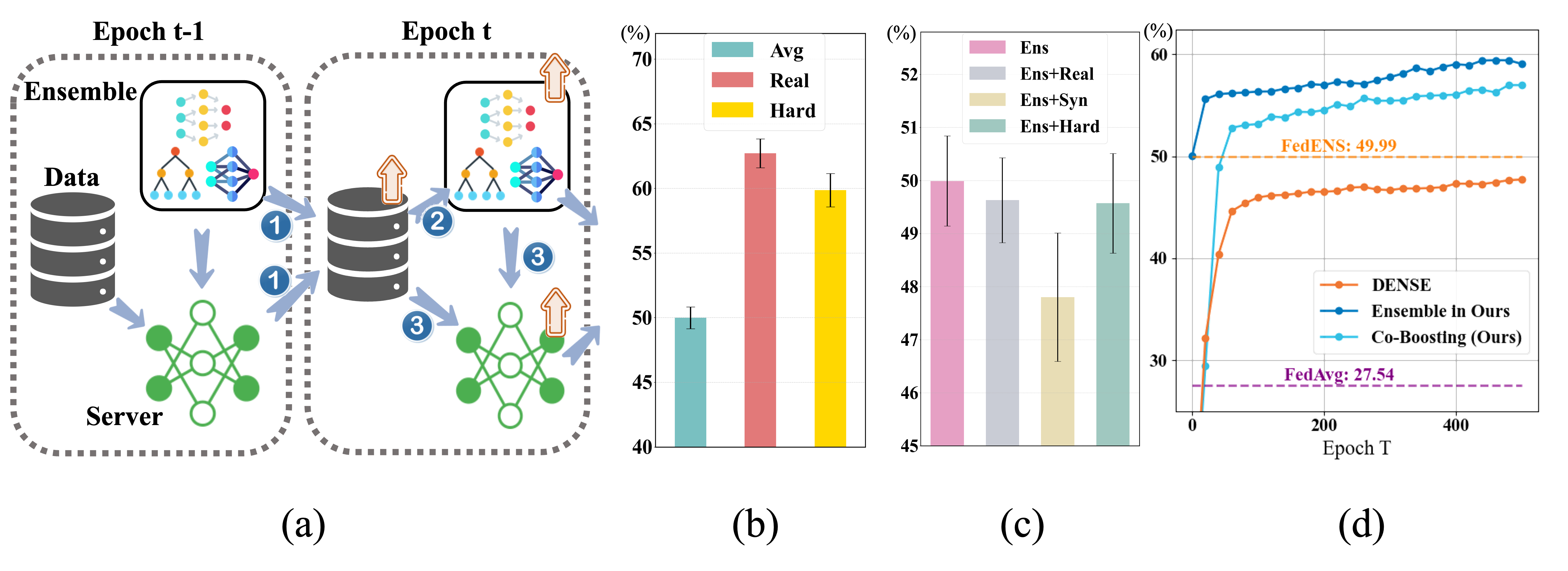
To address these challenges, we propose Co-Boosting, a novel one-shot federated learning algorithm as in Fig. 1(a), in which the synthesized data and the ensemble model mutually boost each other progressively. More specifically, in each training epoch, higher-quality hard samples are generated based on the previous epoch’s ensemble and server model. Based on these hard samples, the aggregation weight for each client model is adjusted, forming a better ensemble. Subsequently, the server model is updated by distilling knowledge from both the enriched data and the refined ensemble. As a result, with the continuous enhancement of both data and the ensemble, the final server model naturally improves. As depicted in Fig. 1(b), (c), and (d), with a better weighted ensemble model and better-quality hard samples, Co-boosting naturally achieves state-of-art performance.
Thorough experiments on multiple benchmark datasets demonstrate the superiority of the proposed Co-Boosting. What’s more, due to its inherent nature, our proposed Co-Boosting is more practical to today’s model market scenarios. In summary, our main contributions can be summarized as follows: 1) We demonstrate that it is possible to simultaneously improve the quality of the synthesized data and the ensemble, which are two key elements in OFL. This discovery could spur progress in OFL methods, highlighting the need to optimize their interaction. 2) Within an adversarial paradigm, we introduce Co-Boosting, a novel one-shot federated learning method. Periodically, in Co-Boosting, hard samples are generated from the current ensemble, which, in turn, are used to reweight clients, forming an improved ensemble. This mutual enhancement of synthetic data quality and the ensemble collectively contributes to the natural emergence of a high-performing distilled server model. 3) Our proposed method Co-Boosting, is highly practical to the contemporary model market scenarios as it eliminates the necessity for client-side training adjustments, entails no extra data or model transmissions, and accommodates diverse client model architectures. 4) Extensive experiments confirm the effectiveness of Co-Boosting, consistently outperforming other baselines thanks to the improved quality of both the synthetic data and ensemble.
2 Related Works
2.1 One-shot Federated learning
Guha et al. (2019) originally proposes OFL which collects local models as an ensemble for the final prediction and further proposes to use knowledge distillation (KD) on such ensemble with public data. This paradigm, which is followed by most works, inherently relates the performance of the server model to the data and ensemble used in the KD stage. Li et al. (2021) proposes to improve the ensemble on the public data. Instead of using public data, Zhou et al. (2020) proposes to transmit the distilled local dataset for the server, Yang et al. (2023) proposes to use auxiliary pre-trained diffusion model, while Zhang et al. (2022a) generates fake data scouring from the direct ensemble. Regarding the improvement of the ensemble, Dennis et al. (2021) utilizes a cluster-based method and requires uploading the cluster means. Diao et al. (2023) and Heinbaugh et al. (2023) modify the local training phase of each client by introducing placeholders, or conditional variation auto-encoders. However, none of the aforementioned methods simultaneously address improvements in both data and the ensemble. Moreover, few works can be practically applied, especially in contemporary model-market scenarios (Vartak et al., 2016) where only well-pretrained models are provided to the server. This situation implies constraints such as no alterations to the client’s local training, no additional transmissions, and the possibility of client model heterogeneity.
2.2 Knowledge Distillation
Knowledge distillation (KD) (Hinton et al., 2015) is proposed to transfer knowledge from one or more networks (teacher) to another (student). Taking the same spirit, KD in federated learning focuses on transferring knowledge from multiple local clients to the global server model. Lin et al. (2020) initially introduced to utilize KD at the server side based on an unlabeled auxiliary dataset. In an effort to reduce reliance on proxy datasets, generators that are locally updated and globally aggregated are used in Zhu et al. (2021) and Zhang et al. (2022b) to synthesize distillation samples. Wang et al. (2023) further enhances the basic ensemble distillation by using weighted averaging based on locally trained discriminators. However, in the context of OFL, conducting multiple rounds of training or transmitting generators and discriminators is not practical. Additionally, the need for an additional local client component violates the constraints in modern model-market OFL settings. More seriously, the generator trained locally has direct access to the training samples, potentially leading to privacy leakage through its ability to remember all the training data (Liu et al., 2019). On the other hand, the generator in OFL is trained without access to even one single raw data.
3 Methodology
In this section, we first introduce the general process of one-shot federated learning (OFL). Then we detail the proposed method, Co-Boosting, in how we generate high-quality data, high-quality ensemble, and how to link and make them boost each other as illustrated in Fig. 1(a).
3.1 One-Shot Federated Learning
Suppose we have a set of clients , with clients in total. Each client has a local private dataset , where is the number of local data samples with the corresponding label . OFL’s goal is to train a good machine learning model with parameter over with the help of a server in only one communication, as in
| (1) |
where is the cross-entropy function, is the prediction function of the server that outputs the logits (i.e., outputs of the last fully connected layer) of given parameter .
Noticeably, in one-shot federated learning, the original training set cannot be accessed, and only well-pretrained models parameterized by , are provided. Here, we define the ensemble as:
| (2) |
where denotes the prediction function that output the logits of given , while adjusts the weights of each local client logits. When , the ensemble is the same as the averaged ensemble, while when , the ensemble becomes weighted according to the data amount. For simplicity, in the rest paper, we use to denote the ensemble and to denote , which means the output logits of the ensemble given .
When aggregating pre-trained models into one server model , existing works mostly follow a two-stage framework. The first is to synthesize data based on the ensemble output. In particular, giving a random noise sampled from a standard Gaussian distribution and a random uniformly sampled label , the generator with is responsible for generating the data , forming the synthetic dataset . Typically, to make sure the synthetic data can be classified correctly with a high probability by the ensemble , the following loss is adopted:
| (3) |
After getting the synthetic dataset based on the generator in Eq.(3), OFL intends to distill the ensemble into the final server model with the help of these synthetic data, as in:
| (4) |
where denotes the Kullback-Leibler (KL) divergence.
Existing works illustrate that the performance of the server model is intrinsically related to the synthetic data and the ensemble , which can also be concluded according to Eq.(4).
3.2 Boosting the data quality
Synthesizing data is used to distill the ensemble model into the final server model as in Eq.(4). The quality of these synthesized data has been demonstrated vital to the distillation stage Lin et al. (2020). Moreover, since these data are also generated sourcing from the ensemble as in Eq.(3), it is of great importance to make these data embed as much the knowledge of the ensemble as possible and make them transferable to the final server model.
However, as hinted in Wang et al. (2020) and Zhang et al. (2022a), by utilizing only the CE loss, the synthesized data can be easily fitted by the server model, resulting in poor performance in the knowledge distillation stage. Therefore, to improve the quality of the generated data and make them focus more on transferable components, taking inspiration from Dong et al. (2020) and Li et al. (2023a), we increase the importance of hard samples while suppressing the importance of easy-to-fit samples in the generation stage. More specifically, given a prediction function which output logits, we employ the GHM introduced in Li et al. (2019) to measure the sample difficulty of :
| (5) |
where is the probability on label predicted by the function with . Built upon the sample difficulty, we propose a hard-sample-enhanced loss to synthesize data:
| (6) |
Moreover, to make synthesized samples hard for the server model to fit, an adversarial loss (Zhang et al., 2022c) is also introduced to generate hard samples. We try to maximize the differences in predictions between the ensemble model and the server model when generating data as follows:
| (7) |
By combining the above losses, we can obtain the loss used to train the generator as follows:
| (8) |
where is the scaling factor for the losses, which is set as 1 in the implementations.
Though samples synthesized using Eq.(8) are hard to fit for the current ensemble model, their difficulties for the server model are still lacking. This stems from the fact that the server model can easily fit these limited unchanged data during multiple distillation steps. To further promote the sample difficulty and diversity on the fly, we draw inspiration from adversarial learning (Goodfellow et al., 2014; Tashiro et al., 2020) to generate hard and diverse samples for the server model to learn.
More specifically, we diverse and increase the sample difficulty on the fly to make the synthetic samples hard to fit by introducing a perturbation for each :
| (9) |
where represents the -norm and controls the strength of perturbation. To simplify the computation and enhance the diversity, instead of the iterative adversarial attacks, we take only one step of loss backward to seek the direction in the input space that maximizes the similarity between the model output and a randomly sampled vector. The hard samples are constructed as follows:
| (10) |
where is a randomly sample vector with dimension . Following these, the originally generated hard samples are further harder and more diverse due to the randomness in .
By replacing each sample in into , we can achieve a more hard and diverse synthetic dataset . Utilizing these hard samples, the knowledge of the ensemble model is transferred to the server model with parameter by knowledge distillation the same as in Eq.(4).
Overall, with the hard sample technique embedding in the data synthesizing stage (replacing the generator loss in Eq.(3) with Eq.(8) and making them diverse in the distillation stage (reconstruct the synthetic dataset according to Eq.(10)), the quality of data generated and used for distillation becomes better, naturally boosting the performance of the server model.
3.3 Boosting the ensemble quality
The ensemble model takes the role of aggregating knowledge from all pre-trained models and forms a virtually best-performance teacher. A straightforward method is to obtain the global model by averaging the parameters of all client models (e.g. FedAvg (McMahan et al., 2017)). However, FedAvg may fail to deliver a good performance when data among clients are non-IID (Karimireddy et al., 2020; Acar et al., 2021) and cannot handle the challenge of client model heterogeneity. Recent works (Heinbaugh et al., 2023; Diao et al., 2023) intend to construct a better ensemble model by altering the local training phase of each client, which may be unreliable, especially in today’s model market scenarios. To tackle the client model heterogeneity and make the ensemble more practical, Guha et al. (2019); Zhang et al. (2022a) utilizes the direct ensemble with as the teacher, which means averaging the logits or weighted averaging them according to the number of the client data (). However, as suggested by Zhang et al. (2023) and Wang et al. (2023), the simple averaging or weighted averaging based on the client data amount may not be effective, especially in non-IID settings. There exists a better weighted combination of each client’s contribution. Yet, their methods either need to alter the local training or transmit additional information, therefore their methods cannot be applied to one-shot FL.
To this end, we propose to boost the ensemble quality by searching for a more effective weighted ensemble of logits. As demonstrated by our experimental results in Fig. 1(b), given high-quality data (validation data), we can achieve a better ensemble with weights different from simple averaging or data amount based averaging. Fortunately, instead of using auxiliary data, we actually can acquire high-quality generated data from the hard synthesized samples set . Therefore, to get the best weights on , we need to solve the following optimization problem:
| (11) |
where is the corresponding label to each synthesized hard samples . Exploring the optimal requires multiple inner steps, leading to the training time to increase exponentially. Also inspired by methods of adversarial attacks (Goodfellow et al., 2014), we use the gradient’s direction and fixed step size to update every time after getting each batch of the synthesized data :
| (12) |
where denotes bounding each into and means the sign function.
The reweighting of each client’s logit results in a superior ensemble model, which will naturally benefit the server model. Moreover, since the operations are done on the logit layer, this reweighting technique can be easily applied to both heterogeneous and homogeneous client model settings.
3.4 Co-boosting the data and the ensemble
As aforementioned, we introduce how to boost the data quality by utilizing hard sample techniques with a fixed ensemble and how to boost the ensemble with a fixed synthetic dataset. Actually, these two stages are inherently entangled and can boost each other at the same time. To get high-quality ensemble and synthesized data , we are in fact trying to solve the following problem:
| (13) |
where is the label of sample , is the perturbation constrained in . This problem can be addressed adversarially, which means the improvement of the data and the ensemble can be done simultaneously. With better quality data, the weighted ensemble can reach higher performance, while with this better ensemble, the data synthesized sourcing from this ensemble can further embed more knowledge. Therefore, by mutually boosting the quality of the synthesized data and the ensemble, we can naturally get a better-performance server model through the distillation in Eq.(4).
The overall algorithm is summarized in Algorithm 1. In each epoch, we first generate hard samples based on the current ensemble model and the last epoch server model. With these generated data, an enhanced ensemble model is cultivated by searching for the optimal ensembling weights of each client’s logits. Utilizing the generated data and the upgraded ensemble, the final server model is trained by distilling the ensemble on these data. As illustrated in Sec. 3.2 and Sec. 3.3, with either one fixed, one can benefit from the other, thus by mutually boosting each other in the proposed Co-Boosting, we can achieve both better quality data and the ensemble periodically. Therefore, the global server model trained on them will inherently become better than other methods.
4 Experiments
4.1 Experimental Details
Datasets and partitions. We conduct experiments on five real-world image datasets that are standard in the FL literature: MNIST (LeCun et al., 1998), FMNIST (Xiao et al., 2017), SVHN (Netzer et al., 2011), CIFAR10, and CIFAR100 (Krizhevsky et al., 2009). To simulate statistical heterogeneity, we use Dirichlet distribution to generate disjoint non-IID client training datasets as in Zhang et al. (2022a) and Heinbaugh et al. (2023). In particular, we sample and allocate a proportion of the data of class to client . The parameter controls the level of statistical imbalance, with a smaller inducing more skewed label distributions among clients.
Baselines. Within the contemporary model-market scenarios, we compare the performance of Co-Boosting111Code is available at https://github.com/rong-dai/Co-Boosting against two existing methods: FedAvg (McMahan et al., 2017) and DENSE (Zhang et al., 2022a). Similar in (Zhang et al., 2022a), we also introduce two prevailing data-free KD methods DAFL (Chen et al., 2019) and ADI (Yin et al., 2020) and apply these to one-shot FL, giving F-DAFL and F-ADI. We also include FedDF (Lin et al., 2020) using the real validation dataset as the baseline.
Configurations. Following McMahan et al. (2017), we use CNN with 5 layers for SVHN, CIFAR10, and CIFAR100, LeNet-5 (LeCun et al., 1998) for MNIST and FMNIST. All available test data is used to evaluate the final server model (or ensemble). Unless otherwise stated, experiments are done with 10 clients and -parted. Results are reported averaged across at least 3 random seeds.
4.2 General Results
Method FedAvg FedDF F-ADI F-DAFL DENSE Co-Boosting MNIST 0.05 46.350.98 80.731.08 80.121.76 78.491.36 81.061.12 93.930.69 0.1 75.680.82 87.910.92 85.920.82 87.440.61 87.831.38 94.441.02 0.3 78.970.82 97.660.10 96.340.83 96.360.98 96.960.53 97.250.44 FMNIST 0.05 20.071.98 44.730.40 42.252.01 41.660.83 44.771.87 50.621.13 0.1 46.611.94 68.401.80 63.191.99 67.810.93 69.431.94 74.861.70 0.3 60.132.62 83.140.47 74.801.72 78.680.49 81.310.83 83.111.28 SVHN 0.05 39.412.19 60.790.52 56.581.05 59.381.19 60.241.31 65.400.86 0.1 46.221.92 68.980.63 66.331.69 67.770.34 68.301.01 72.881.19 0.3 72.612.06 79.780.55 76.751.47 78.011.02 78.730.84 81.311.09 CIFAR- 10 0.05 17.492.51 37.530.67 36.941.70 37.821.30 38.371.08 47.200.81 0.1 27.541.80 49.630.80 47.190.97 46.320.97 47.801.21 57.090.94 0.3 46.392.37 67.180.60 60.601.32 65.891.69 66.771.55 70.241.56 CIFAR- 100 0.05 6.450.92 16.070.54 13.751.01 15.790.21 16.171.33 19.241.42 0.1 10.281.70 22.070.43 19.441.66 20.991.17 22.211.41 23.591.27 0.3 15.222.08 30.710.53 26.141.37 28.791.25 30.331.24 31.301.30
Overall Comparison. To evaluate the effectiveness of our method, we conduct experiments under various non-IID settings by varying and report the performance across different datasets and methods in Table 1. Notice, that we use the validation set in FedDF, which is not practical in the real world. From the table, we can conclude that Co-Boosting consistently outperforms all other baselines in all settings. Notably, in many settings, Co-Boosting achieves over a 5% accuracy improvement compared to the best baseline, DENSE. In cases of extreme statistical heterogeneity, such as when , Co-Boosting surpasses the best baseline by substantial margins with 12.87%, 5.85%, 5.16%, 8.83%, and 3.07% on MNIST, FMNIST, SVHN, CIFAR-10, and CIFAR-100, respectively. We also compare the performance of the ensemble used in different methods on SVHN and CIFAR-10 in Table 2, others please refer to the Appendix. FedENS denotes averaged ensemble. The superior performance of the server model can be attributed to the enhanced quality of synthesized data and the ensemble. While all compared methods, except FedAvg, utilize the direct logits averaging ensemble as the ensemble and aim to distill knowledge from it in a data-free manner, Co-Boosting, with its co-enhancing technique, results in a superior ensemble teacher, surpassing FedENS significantly. In a word, the superiority of our proposed method can be owed to the enhanced data and ensemble quality, which naturally translates into a better server model.
| Dataset | SVHN | CIFAR-10 | ||||
|---|---|---|---|---|---|---|
| Method | =0.05 | =0.1 | =0.3 | =0.05 | =0.1 | =0.3 |
| FedENS | 61.621.61 | 69.710.68 | 80.540.57 | 42.340.67 | 49.990.85 | 69.610.50 |
| Co-Boosting | 65.691.48 | 73.521.71 | 82.901.35 | 48.751.25 | 59.861.76 | 72.671.27 |
Adaptation to Client Model Heterogeneity. To evaluate our proposed method in a potential client heterogeneity setting, we apply five different models under a CIFAR-10, -parted setting. The heterogeneous models include CNN1 in McMahan et al. (2017), CNN2 in the pytorch tutorial (Paszke et al., 2019), ResNet (He et al., 2016), MobileNet (Howard et al., 2019), and ShuffleNet (Ma et al., 2018). Table 3 demonstrates the results of comparable methods, where Local denotes directly taking the pre-trained model for testing. We take ResNet as the server architecture and omit FedAvg as it does not support this setting. We use the same optimization hyperparameter for all methods and across all model architectures. We remark that as suggested in Zhang et al. (2022a) and Diao et al. (2021), FL under both non-IID data and different model architecture is a quite challenging task. Even under this setting, our proposed Co-Boosting still consistently outperforms other baselines by a large margin thanks to the benefits of making the ensemble and data improve together.
| Local | FedDF | F-ADI | F-DAFL | DENSE | Co-Boosting | |
|---|---|---|---|---|---|---|
| =0.05 | 46.491.97 | 56.511.87 | 55.641.96 | 55.141.51 | 55.791.75 | 58.641.83 |
| =0.1 | 51.701.14 | 59.491.06 | 60.301.70 | 58.581.49 | 58.670.88 | 62.300.90 |
| =0.3 | 67.611.54 | 70.531.19 | 71.611.24 | 71.921.95 | 72.981.61 | 75.021.37 |
4.3 In-depth Study
Different Local Data Amount. To further assess the effectiveness of Co-Boosting, which involves a better-weighted ensemble, we conduct experiments in an unbalanced local data setting. Similar to Acar et al. (2021), we sample data amounts for each client from a lognormal distribution. Higher values of result in more unequal data distribution. Table 4 and Fig. 2 display the performance of the ensemble and the server, where the prefix ’DW-’ signifies weighted averaging based on the local data amount. As observed, reweighting clients based on their data amount yields some benefits, but it falls short of achieving the best ensemble. Furthermore, when using the averaged ensemble FedENS as the teacher, all baseline methods perform poorly due to the suboptimal teacher. In contrast, benefiting from simultaneously boosting data and ensemble, the ensemble we get consistently outperforms FedENS. This leads to a substantial performance gain of the server model achieved in Co-Boosting over all baselines, with a margin of at least 10%.
Method =0.4 =0.8 =1.2 FedENS 46.871.02 41.861.20 37.881.38 DW-FedENS 47.801.21 53.250.52 47.520.40 Co-Boosting 58.940.50 57.411.12 55.271.72
![[Uncaptioned image]](/html/2402.15070/assets/x1.png)
Different Data Distribution Shift. Following Diao et al. (2023), we also conduct experiments on a partition setting, which means each client only possesses data of out of all classes. Results in Table 5 further demonstrate the superiority of our proposed method. With better data quality and better ensemble, our method consistently achieves the best server model.
| FedAvg | FedDF | F-ADI | F-DAFL | DENSE | Co-Boosting | |
|---|---|---|---|---|---|---|
| 2 | 16.152.61 | 23.070.83 | 23.161.12 | 24.530.57 | 23.850.93 | 36.371.85 |
| 3 | 26.471.46 | 38.390.64 | 36.061.93 | 38.131.17 | 38.141.38 | 53.911.80 |
| 4 | 33.782.42 | 54.511.12 | 51.041.40 | 52.530.97 | 51.531.79 | 58.001.59 |
| 5 | 35.951.96 | 58.341.58 | 55.272.06 | 54.671.26 | 56.791.03 | 62.521.75 |
Different Number of Clients. We evaluate the performance of these methods by varying the number of clients participating in OFL in Table 6. From the table, the final sever model still achieves the best accuracy when increasing the number of clients. This again validates that the increment quality of the ensemble model and data naturally brings a better server model.
| FedAvg | FedDF | F-ADI | F-DAFL | DENSE | Co-Boosting | |
|---|---|---|---|---|---|---|
| 5 | 36.941.74 | 50.620.98 | 48.760.78 | 49.761.42 | 50.531.02 | 54.291.38 |
| 10 | 27.541.80 | 49.630.80 | 47.190.97 | 46.320.97 | 47.801.21 | 57.090.94 |
| 20 | 26.341.97 | 38.980.99 | 38.930.64 | 36.281.39 | 38.860.42 | 49.560.98 |
| 50 | 23.010.94 | 29.520.62 | 27.451.13 | 29.410.90 | 28.510.54 | 42.291.43 |
Effects of the proposed components. We further study the effectiveness of our proposed hard sample generation loss in Sec.3.2, on-the-fly sample difficulty promotion in Sec.3.2, and ensemble enhancing in Sec.3.3. Table 7 shows the experimental results on SVHN and CIFAR-10 in a 10-client parted setting. The results in the table illustrate that individually improving either data or ensemble leads to noticeable enhancements in the final server model performance. However, the most remarkable results are achieved when both data quality and ensemble capability are improved simultaneously. This finding strongly aligns with the underlying motivation of our study.
| GHS | DHS | EE | SVHN | CIFAR-10 |
|---|---|---|---|---|
| 58.46 | 39.72 | |||
| ✔ | 61.18 | 42.85 | ||
| ✔ | 61.38 | 43.75 | ||
| ✔ | 62.67 | 41.45 | ||
| ✔ | ✔ | 63.42 | 45.81 | |
| ✔ | ✔ | 62.46 | 44.36 | |
| ✔ | ✔ | 64.40 | 46.74 | |
| ✔ | ✔ | ✔ | 65.40 | 47.20 |
More facets. For a thorough and comprehensive understanding, we operate sensitivity analyses of hyperparameters, compare with multi-round federated learning, and conduct experiments with heavier local models. Please refer to the Appendix for the results. Moreover, since our Co-Boosting needs no alternation of the local training, it can be combined with advanced local training. The results attached in the Appendix further demonstrate the superiority of our proposed Co-Boosting.
Limitation. The mixing weights are determined using synthetic samples. Though promising, there is still some disparity when compared to a mixing-weighted ensemble trained on real training data, as in Fig. 1(b). One possible way is to introduce virtual data (Tang et al., 2022). The exploration of methods to generate data capable of bridging this gap remains an avenue for further research.
5 Conclusion
In this paper, we seek to tackle the inherent bottleneck of one-shot federated learning, where the performance of the server model is inextricably linked with the quality of the generated data and the ensemble. We propose Co-Boosting, a novel method that facilitates a mutually beneficial relationship between data generation and ensemble improvement. By iteratively generating hard samples from the ensemble and enhancing the ensemble based on these data, Co-Boosting adversarially improves the quality of both the data and the ensemble, leading to the natural refinement of the server model. Extensive experiments across various settings validate the efficacy of our method and demonstrate that our method can be practically applied to contemporary model-market scenarios.
Acknowledgements
RD, YGZ and BH were supported by the NSFC General Program No. 62376235, Guangdong Basic and Applied Basic Research Foundation No. 2022A1515011652, CCF-Baidu Open Fund, HKBU Faculty Niche Research Areas No. RC-FNRA-IG/22-23/SCI/04, and HKBU CSD Departmental Incentive Scheme. RD and XY were supported by National Natural Science Foundation of China (NSFC) under Grant U22A2094. TL is partially supported by the following Australian Research Council projects: FT220100318, DP220102121, LP220100527, LP220200949, IC190100031.
References
- Acar et al. (2021) Durmus Alp Emre Acar, Yue Zhao, Ramon Matas, Matthew Mattina, Paul Whatmough, and Venkatesh Saligrama. Federated learning based on dynamic regularization. In International Conference on Learning Representations, 2021. URL https://openreview.net/forum?id=B7v4QMR6Z9w.
- Caldarola et al. (2022) Debora Caldarola, Barbara Caputo, and Marco Ciccone. Improving generalization in federated learning by seeking flat minima. In European Conference on Computer Vision, pp. 654–672. Springer, 2022.
- Chang et al. (2023a) Tianyu Chang, Xun Yang, Xin Luo, Wei Ji, and Meng Wang. Learning style-invariant robust representation for generalizable visual instance retrieval. In Proceedings of the 31st ACM International Conference on Multimedia, pp. 6171–6180, 2023a.
- Chang et al. (2023b) Tianyu Chang, Xun Yang, Tianzhu Zhang, and Meng Wang. Domain generalized stereo matching via hierarchical visual transformation. In Proceedings of the IEEE/CVF Conference on Computer Vision and Pattern Recognition (CVPR), pp. 9559–9568, June 2023b.
- Chen et al. (2019) Hanting Chen, Yunhe Wang, Chang Xu, Zhaohui Yang, Chuanjian Liu, Boxin Shi, Chunjing Xu, Chao Xu, and Qi Tian. Data-free learning of student networks. In Proceedings of the IEEE/CVF International Conference on Computer Vision, pp. 3514–3522, 2019.
- Chen et al. (2022) Hong-You Chen, Cheng-Hao Tu, Ziwei Li, Han Wei Shen, and Wei-Lun Chao. On the importance and applicability of pre-training for federated learning. In The Eleventh International Conference on Learning Representations, 2022.
- Dai et al. (2022) Rong Dai, Li Shen, Fengxiang He, Xinmei Tian, and Dacheng Tao. Dispfl: Towards communication-efficient personalized federated learning via decentralized sparse training. In International Conference on Machine Learning, pp. 4587–4604. PMLR, 2022.
- Dai et al. (2023) Rong Dai, Xun Yang, Yan Sun, Li Shen, Xinmei Tian, Meng Wang, and Yongdong Zhang. Fedgamma: Federated learning with global sharpness-aware minimization. IEEE Transactions on Neural Networks and Learning Systems, pp. 1–14, 2023. doi: 10.1109/TNNLS.2023.3304453.
- Dennis et al. (2021) Don Kurian Dennis, Tian Li, and Virginia Smith. Heterogeneity for the win: One-shot federated clustering. In International Conference on Machine Learning, pp. 2611–2620. PMLR, 2021.
- Diao et al. (2021) Enmao Diao, Jie Ding, and Vahid Tarokh. Heterofl: Computation and communication efficient federated learning for heterogeneous clients. In International Conference on Learning Representations, 2021. URL https://openreview.net/forum?id=TNkPBBYFkXg.
- Diao et al. (2023) Yiqun Diao, Qinbin Li, and Bingsheng He. Towards addressing label skews in one-shot federated learning. In The Eleventh International Conference on Learning Representations, 2023. URL https://openreview.net/forum?id=rzrqh85f4Sc.
- Dong et al. (2020) Jiahua Dong, Yang Cong, Gan Sun, Bineng Zhong, and Xiaowei Xu. What can be transferred: Unsupervised domain adaptation for endoscopic lesions segmentation. In Proceedings of the IEEE/CVF conference on Computer Vision and Pattern Recognition, pp. 4023–4032, 2020.
- Ganin et al. (2016) Yaroslav Ganin, Evgeniya Ustinova, Hana Ajakan, Pascal Germain, Hugo Larochelle, François Laviolette, Mario Marchand, and Victor Lempitsky. Domain-adversarial training of neural networks. The journal of machine learning research, 17(1):2096–2030, 2016.
- Goodfellow et al. (2014) Ian J Goodfellow, Jonathon Shlens, and Christian Szegedy. Explaining and harnessing adversarial examples. arXiv preprint arXiv:1412.6572, 2014.
- Guha et al. (2019) Neel Guha, Ameet Talwalkar, and Virginia Smith. One-shot federated learning. arXiv preprint arXiv:1902.11175, 2019.
- He et al. (2016) Kaiming He, Xiangyu Zhang, Shaoqing Ren, and Jian Sun. Deep residual learning for image recognition. In Proceedings of the IEEE/CVF conference on Computer Vision and Pattern Recognition, pp. 770–778, 2016.
- Heinbaugh et al. (2023) Clare Elizabeth Heinbaugh, Emilio Luz-Ricca, and Huajie Shao. Data-free one-shot federated learning under very high statistical heterogeneity. In The Eleventh International Conference on Learning Representations, 2023. URL https://openreview.net/forum?id=_hb4vM3jspB.
- Hinton et al. (2015) Geoffrey Hinton, Oriol Vinyals, and Jeff Dean. Distilling the knowledge in a neural network. arXiv preprint arXiv:1503.02531, 2015.
- Howard et al. (2019) Andrew Howard, Mark Sandler, Grace Chu, Liang-Chieh Chen, Bo Chen, Mingxing Tan, Weijun Wang, Yukun Zhu, Ruoming Pang, Vijay Vasudevan, et al. Searching for mobilenetv3. In Proceedings of the IEEE/CVF International Conference on Computer Vision, pp. 1314–1324, 2019.
- Kairouz et al. (2021) Peter Kairouz, H Brendan McMahan, Brendan Avent, Aurélien Bellet, Mehdi Bennis, Arjun Nitin Bhagoji, Kallista Bonawitz, Zachary Charles, Graham Cormode, Rachel Cummings, et al. Advances and open problems in federated learning. Foundations and Trends® in Machine Learning, 14(1–2):1–210, 2021.
- Karimireddy et al. (2020) Sai Praneeth Karimireddy, Satyen Kale, Mehryar Mohri, Sashank Reddi, Sebastian Stich, and Ananda Theertha Suresh. Scaffold: Stochastic controlled averaging for federated learning. In International Conference on Machine Learning, pp. 5132–5143. PMLR, 2020.
- Krizhevsky et al. (2009) Alex Krizhevsky, Geoffrey Hinton, et al. Learning multiple layers of features from tiny images. Master thesis, 2009.
- Le & Yang (2015) Ya Le and Xuan Yang. Tiny imagenet visual recognition challenge. CS 231N, 7(7):3, 2015.
- LeCun et al. (1998) Yann LeCun, Léon Bottou, Yoshua Bengio, and Patrick Haffner. Gradient-based learning applied to document recognition. Proceedings of the IEEE, 86(11):2278–2324, 1998.
- Li et al. (2019) Buyu Li, Yu Liu, and Xiaogang Wang. Gradient harmonized single-stage detector. In Proceedings of the AAAI conference on artificial intelligence, volume 33, pp. 8577–8584, 2019.
- Li et al. (2017) Da Li, Yongxin Yang, Yi-Zhe Song, and Timothy M Hospedales. Deeper, broader and artier domain generalization. In Proceedings of the IEEE international conference on computer vision, pp. 5542–5550, 2017.
- Li et al. (2023a) Huantong Li, Xiangmiao Wu, Fanbing Lv, Daihai Liao, Thomas H Li, Yonggang Zhang, Bo Han, and Mingkui Tan. Hard sample matters a lot in zero-shot quantization. In Proceedings of the IEEE/CVF conference on Computer Vision and Pattern Recognition, pp. 24417–24426, 2023a.
- Li et al. (2021) Qinbin Li, Bingsheng He, and Dawn Song. Practical one-shot federated learning for cross-silo setting. In Zhi-Hua Zhou (ed.), Proceedings of the Thirtieth International Joint Conference on Artificial Intelligence, IJCAI-21, pp. 1484–1490. International Joint Conferences on Artificial Intelligence Organization, 8 2021. doi: 10.24963/ijcai.2021/205. URL https://doi.org/10.24963/ijcai.2021/205. Main Track.
- Li et al. (2020a) Tian Li, Anit Kumar Sahu, Ameet Talwalkar, and Virginia Smith. Federated learning: Challenges, methods, and future directions. IEEE signal processing magazine, 37(3):50–60, 2020a.
- Li et al. (2020b) Tian Li, Anit Kumar Sahu, Manzil Zaheer, Maziar Sanjabi, Ameet Talwalkar, and Virginia Smith. Federated optimization in heterogeneous networks. Proceedings of Machine Learning and Systems, 2:429–450, 2020b.
- Li et al. (2023b) Ying Li, Xingwei Wang, Rongfei Zeng, Praveen Kumar Donta, Ilir Murturi, Min Huang, and Schahram Dustdar. Federated domain generalization: A survey. arXiv preprint arXiv:2306.01334, 2023b.
- Lin et al. (2020) Tao Lin, Lingjing Kong, Sebastian U Stich, and Martin Jaggi. Ensemble distillation for robust model fusion in federated learning. Advances in Neural Information Processing Systems, 33:2351–2363, 2020.
- Liu et al. (2019) Yi Liu, Jialiang Peng, JQ James, and Yi Wu. Ppgan: Privacy-preserving generative adversarial network. In 2019 IEEE 25Th international conference on parallel and distributed systems (ICPADS), pp. 985–989. IEEE, 2019.
- Ma et al. (2018) Ningning Ma, Xiangyu Zhang, Hai-Tao Zheng, and Jian Sun. Shufflenet v2: Practical guidelines for efficient cnn architecture design. In Proceedings of the European conference on computer vision (ECCV), pp. 116–131, 2018.
- McMahan et al. (2017) Brendan McMahan, Eider Moore, Daniel Ramage, Seth Hampson, and Blaise Aguera y Arcas. Communication-efficient learning of deep networks from decentralized data. In Artificial Intelligence and statistics, pp. 1273–1282. PMLR, 2017.
- Mothukuri et al. (2021) Viraaji Mothukuri, Reza M Parizi, Seyedamin Pouriyeh, Yan Huang, Ali Dehghantanha, and Gautam Srivastava. A survey on security and privacy of federated learning. Future Generation Computer Systems, 115:619–640, 2021.
- Netzer et al. (2011) Yuval Netzer, Tao Wang, Adam Coates, Alessandro Bissacco, Bo Wu, and Andrew Y Ng. Reading digits in natural images with unsupervised feature learning. 2011.
- Paszke et al. (2019) Adam Paszke, Sam Gross, Francisco Massa, Adam Lerer, James Bradbury, Gregory Chanan, Trevor Killeen, Zeming Lin, Natalia Gimelshein, Luca Antiga, et al. Pytorch: An imperative style, high-performance deep learning library. Advances in neural information processing systems, 32, 2019.
- Peng et al. (2023) Yixing Peng, Quan Wang, Zhendong Mao, and Yongdong Zhang. Sade: A self-adaptive expert for multi-dataset question answering. In ICASSP 2023-2023 IEEE International Conference on Acoustics, Speech and Signal Processing (ICASSP), pp. 1–5. IEEE, 2023.
- Qiao et al. (2018) Siyuan Qiao, Wei Shen, Zhishuai Zhang, Bo Wang, and Alan Yuille. Deep co-training for semi-supervised image recognition. In Proceedings of the european conference on computer vision (eccv), pp. 135–152, 2018.
- Qu et al. (2022) Zhe Qu, Xingyu Li, Rui Duan, Yao Liu, Bo Tang, and Zhuo Lu. Generalized federated learning via sharpness aware minimization. In International Conference on Machine Learning, pp. 18250–18280. PMLR, 2022.
- Simonyan & Zisserman (2014) Karen Simonyan and Andrew Zisserman. Very deep convolutional networks for large-scale image recognition. arXiv preprint arXiv:1409.1556, 2014.
- Song et al. (2023) Peipei Song, Dan Guo, Xun Yang, Shengeng Tang, Erkun Yang, and Meng Wang. Emotion-prior awareness network for emotional video captioning. In Proceedings of the 31st ACM International Conference on Multimedia, pp. 589–600, 2023.
- Tang et al. (2022) Zhenheng Tang, Yonggang Zhang, Shaohuai Shi, Xin He, Bo Han, and Xiaowen Chu. Virtual homogeneity learning: Defending against data heterogeneity in federated learning. In International Conference on Machine Learning, pp. 21111–21132. PMLR, 2022.
- Tashiro et al. (2020) Yusuke Tashiro, Yang Song, and Stefano Ermon. Diversity can be transferred: Output diversification for white-and black-box attacks. Advances in neural information processing systems, 33:4536–4548, 2020.
- Vartak et al. (2016) Manasi Vartak, Harihar Subramanyam, Wei-En Lee, Srinidhi Viswanathan, Saadiyah Husnoo, Samuel Madden, and Matei Zaharia. Modeldb: a system for machine learning model management. In Proceedings of the Workshop on Human-In-the-Loop Data Analytics, pp. 1–3, 2016.
- Wang et al. (2021) Derui Wang, Chaoran Li, Sheng Wen, Surya Nepal, and Yang Xiang. Man-in-the-middle attacks against machine learning classifiers via malicious generative models. IEEE Transactions on Dependable and Secure Computing, 18(5):2074–2087, 2021. doi: 10.1109/TDSC.2020.3021008.
- Wang et al. (2023) Haozhao Wang, Yichen Li, Wenchao Xu, Ruixuan Li, Yufeng Zhan, and Zhigang Zeng. Dafkd: Domain-aware federated knowledge distillation. In Proceedings of the IEEE/CVF conference on Computer Vision and Pattern Recognition, pp. 20412–20421, 2023.
- Wang et al. (2020) Jianyu Wang, Qinghua Liu, Hao Liang, Gauri Joshi, and H Vincent Poor. Tackling the objective inconsistency problem in heterogeneous federated optimization. Advances in neural information processing systems, 33:7611–7623, 2020.
- Xiao et al. (2017) Han Xiao, Kashif Rasul, and Roland Vollgraf. Fashion-mnist: a novel image dataset for benchmarking machine learning algorithms. arXiv preprint arXiv:1708.07747, 2017.
- Yang et al. (2023) Mingzhao Yang, Shangchao Su, Bin Li, and Xiangyang Xue. Exploring one-shot semi-supervised federated learning with a pre-trained diffusion model. arXiv preprint arXiv:2305.04063, 2023.
- Yang et al. (2021) Xun Yang, Fuli Feng, Wei Ji, Meng Wang, and Tat-Seng Chua. Deconfounded video moment retrieval with causal intervention. In Proceedings of the 44th International ACM SIGIR Conference on Research and Development in Information Retrieval, pp. 1–10, 2021.
- Yang et al. (2022) Xun Yang, Shanshan Wang, Jian Dong, Jianfeng Dong, Meng Wang, and Tat-Seng Chua. Video moment retrieval with cross-modal neural architecture search. IEEE Transactions on Image Processing, 31:1204–1216, 2022.
- Yin et al. (2020) Hongxu Yin, Pavlo Molchanov, Jose M Alvarez, Zhizhong Li, Arun Mallya, Derek Hoiem, Niraj K Jha, and Jan Kautz. Dreaming to distill: Data-free knowledge transfer via deepinversion. In Proceedings of the IEEE/CVF conference on Computer Vision and Pattern Recognition, pp. 8715–8724, 2020.
- Yin et al. (2021) Hongxu Yin, Arun Mallya, Arash Vahdat, Jose M Alvarez, Jan Kautz, and Pavlo Molchanov. See through gradients: Image batch recovery via gradinversion. In Proceedings of the IEEE/CVF conference on Computer Vision and Pattern Recognition, pp. 16337–16346, 2021.
- Zhang et al. (2022a) Jie Zhang, Chen Chen, Bo Li, Lingjuan Lyu, Shuang Wu, Shouhong Ding, Chunhua Shen, and Chao Wu. Dense: Data-free one-shot federated learning. Advances in Neural Information Processing Systems, 35:21414–21428, 2022a.
- Zhang et al. (2022b) Lin Zhang, Li Shen, Liang Ding, Dacheng Tao, and Ling-Yu Duan. Fine-tuning global model via data-free knowledge distillation for non-iid federated learning. In Proceedings of the IEEE/CVF conference on Computer Vision and Pattern Recognition, pp. 10174–10183, 2022b.
- Zhang et al. (2023) Ruipeng Zhang, Qinwei Xu, Jiangchao Yao, Ya Zhang, Qi Tian, and Yanfeng Wang. Federated domain generalization with generalization adjustment. In Proceedings of the IEEE/CVF Conference on Computer Vision and Pattern Recognition, pp. 3954–3963, 2023.
- Zhang et al. (2022c) Yonggang Zhang, Mingming Gong, Tongliang Liu, Gang Niu, Xinmei Tian, Bo Han, Bernhard Schölkopf, and Kun Zhang. Adversarial robustness through the lens of causality. In International Conference on Learning Representations, 2022c.
- Zhou et al. (2023) Sheng Zhou, Dan Guo, Jia Li, Xun Yang, and Meng Wang. Exploring sparse spatial relation in graph inference for text-based vqa. IEEE Transactions on Image Processing, 32:5060–5074, 2023. doi: 10.1109/TIP.2023.3310332.
- Zhou et al. (2020) Yanlin Zhou, George Pu, Xiyao Ma, Xiaolin Li, and Dapeng Wu. Distilled one-shot federated learning. arXiv preprint arXiv:2009.07999, 2020.
- Zhu et al. (2021) Zhuangdi Zhu, Junyuan Hong, and Jiayu Zhou. Data-free knowledge distillation for heterogeneous federated learning. In International conference on machine learning, pp. 12878–12889. PMLR, 2021.
- Zhuang et al. (2023) Weiming Zhuang, Chen Chen, and Lingjuan Lyu. When foundation model meets federated learning: Motivations, challenges, and future directions. arXiv preprint arXiv:2306.15546, 2023.
Appendix A More discussions about related works
A.1 One-shot federated learning
Large-scale data is beneficial to service providers in areas such as computer vision (Chang et al., 2023b; a), natural language processing (Peng et al., 2023), or video processing (Yang et al., 2021; 2022; Zhou et al., 2023; Song et al., 2023) among many others who can improve AI-based products or user experience via deep learning techniques with large data requirements. With the growing concern of data privacy, federated learning (FL) (McMahan et al., 2017) allows multiple decentralized clients to collectively train a machine learning model without the need to gather all clients’ data. Most FL algorithms follow the communication prototype of FedAvg (McMahan et al., 2017), which requires many communication rounds to train an effective global. To minimize communication costs and mitigate potential security risks associated with multi-round communications, one-shot federated learning (OFL) has emerged as a promising research direction.
Compared to the straightforward baseline of parameter averaging, as in FedAvg (McMahan et al., 2017), Guha et al. (2019) is the first to propose OFL and utilizes the ensemble of each client’s pre-trained models as the ensemble teacher. Subsequently, an auxiliary dataset is employed to distill knowledge from this ensemble and consolidate it into a unified server model. This paradigm, which is the mainstream of OFL, inherently relates the performance of the server to the data and ensemble used in the knowledge distillation stage.
With the purpose of using high-quality data, Li et al. (2021) proposes a two-tier knowledge distillation stage with the public dataset. Instead of using public data, Zhou et al. (2020) proposes to distill the local dataset on the client side and then send it to the server, which may help the aggregation. Yang et al. (2023) proposes to transmit class prototype and utilize auxiliary pre-trained diffusion models. To avoid transmitting additional information, Zhang et al. (2022a) proposes to generate fake data scouring from the direct ensemble and then use these fake data to distill the server model.
Regarding the improvement of the ensemble, Dennis et al. (2021) reforms the OFL task by utilizing a cluster-based method and requires uploading the cluster means. Diao et al. (2023) modify the local training phase of each client by introducing the placeholders in each client model. Heinbaugh et al. (2023) alters the local model into conditional variation auto-encoders and uses these to generate samples for ensemble and knowledge distillation. Nevertheless, it’s worth noting that none of the previously mentioned approaches tackle enhancements in both data and ensemble simultaneously. Furthermore, only a few methods are applicable in real-world scenarios, particularly in the context of modern model-market scenarios (Vartak et al., 2016), where the server is supplied with exclusively well-pretrained models. In this context, there are constraints that include maintaining the integrity of the client’s local training process, avoiding additional data transmissions, and accommodating potential variations in client model heterogeneity.
We compare these OFL algorithms in Table 8. Noticeably, we are the first to simultaneously enhance both data and ensemble, and our approach is adaptable to contemporary model-market scenarios.
Method Purpose Limitations of contemporary model-market scenarios Improve data Improve ensemble No support of extra data No alternations of local training No additional transmission Adapt to model heterogeneity (Guha et al., 2019) ✗ ✔ ✔ ✗ (Zhou et al., 2020) ✔ ✔ ✔ ✗ ✗ (Li et al., 2021) ✔ ✗ ✗ ✔ ✔ (Dennis et al., 2021) ✔ ✔ ✗ ✗ ✗ (Zhang et al., 2022a) ✔ ✔ ✔ ✔ ✔ (Diao et al., 2023) ✔ ✔ ✗ ✔ ✔ (Heinbaugh et al., 2023) ✔ ✔ ✗ ✗ ✔ (Yang et al., 2023) ✔ ✗ ✗ ✗ ✔ Co-Boosting (ours) ✔ ✔ ✔ ✔ ✔ ✔
A.2 knowledge distillation
Knowledge distillation (KD) (Hinton et al., 2015) is proposed to transfer knowledge from one or more networks (teacher) to another (student). Typically, the student model is trained by minimizing the discrepancy between student and teacher logits generated using a suitable auxiliary dataset; KL-divergence is often chosen as the measure of the discrepancy.
In the same vein, Knowledge Distillation (KD) in federated learning aims to transfer knowledge from multiple local clients to a global server model. This concept was initially introduced by Lin et al. (2020) which proposed using KD at the server side based on an unlabeled auxiliary dataset. To reduce dependency on proxy datasets, researchers have turned to data-free knowledge distillation methods used in centralized settings, such as those proposed in Chen et al. (2019) and Yin et al. (2020). In the centralized setting, a generator or noise is optimized to mimic the behavior of the teacher model. These synthetic data are then used for knowledge distillation. Inspired by these centralized data-free KD works, generators are updated locally and aggregated globally to synthesize distillation samples, as demonstrated in the works Zhu et al. (2021) and Zhang et al. (2022b). Wang et al. (2023) further improved upon basic ensemble distillation by implementing weighted averaging based on locally trained discriminators.
However, in one-shot federated learning (OFL), conducting multiple rounds of training or transmitting generators and discriminators is not practical. Moreover, the requirement for an additional local client component contradicts the constraints in modern model-market OFL settings. A more serious concern is that a locally trained generator has direct access to the training samples, which could potentially lead to privacy leakage as it has the ability to remember all the training data Liu et al. (2019). In contrast, the generator in OFL is trained without access to even a single raw data point.
A.3 More discussions
The parallels and contrasts with centralized co-learning techniques, such as those discussed in Qiao et al. (2018), are indeed intriguing to explore. It’s important to note that centralized co-learning typically operates under the premise of learning from data that presents different views. However, in the one-shot federated learning context, the divergence in data distributions among clients is significantly more pronounced. Moreover, in OFL, models provided to the server are already pre-trained, which precludes the possibility of retraining local models. This distinction is crucial for understanding the unique challenges and approaches in OFL.
Additionally, viewing OFL through the lens of today’s pre-trained foundation model era, as highlighted in works like Chen et al. (2022); Zhuang et al. (2023) opens up new avenues of exploration. Our work positions itself as a pioneering effort in adapting OFL to the era of foundation models. The key strength of our method is its independence from alterations in local training and its architecture-agnostic nature. This flexibility is particularly relevant in the context of foundation models, which are becoming increasingly central in various domains.
Appendix B More experiments
B.1 More details about the Experiment Configuration
Dataset. We use five datasets in our experiments. MNIST (LeCun et al., 1998) is a large database of 10-class handwritten digits. It consists of 60,000 training images and 10,000 testing images, each of which is a 28x28 grayscale image. FMNIST (Xiao et al., 2017) is a dataset of Zalando’s 10-class article images. It consists of a training set of 60,000 examples and a test set of 10,000 examples, each of which is a 28x28 grayscale image. SVHN (Netzer et al., 2011) is a real-world image dataset in 10 classes with a size of 32x32 used for developing machine learning and object recognition algorithms, 72,357 for train, and 26,032 for test. CIFAR-10 (Krizhevsky et al., 2009) consists of 60,000 32x32 color images in 10 classes, 50,000 for train, and 10,000 for test, while CIFAR-100 dataset is similar to the CIFAR-10 dataset but it has 100 classes containing 600 images each. Each image is also a 32x32 color image. For the FedDF method, we use 20% of the training set as a validation set for distillation. While all of the test data is used for testing.
Baselines. To accommodate the contemporary model-market scenarios as seen in Table 8, we compare the performance of Co-Boosting against two existing methods: FedAvg (McMahan et al., 2017) and DENSE (Zhang et al., 2022a). To ensure fair comparisons, we omit comparisons with methods that require the use of auxiliary public datasets, such as Li et al. (2021), or the modification of the local training phases of each client, as seen in Diao et al. (2023) and Heinbaugh et al. (2023). Both of these approaches may not be applicable in real-world scenarios. Moreover, since there is only one communication round, standard FL algorithms based on regularization terms including FedProx (Li et al., 2020b), SCAFFOLD (Karimireddy et al., 2020), and FedDyn (Acar et al., 2021) have no effect. Furthermore, since data-free one-shot FL can be addressed simply by operating data-free KD methods on the direct ensemble model of all models, similar in (Zhang et al., 2022a), we also introduce two prevalent data-free KD methods DAFL (Chen et al., 2019) and ADI (Yin et al., 2020) resulting in F-DAFL and F-ADI. More specifically, F-DAFL and F-ADI aim to either optimize a generator or a noise to mimic the performance of the ensemble teacher model. The data generated from this process is then utilized to distill knowledge into the student (server) model. Additionally, we include FedDF (Lin et al., 2020) using the validation dataset.
Hyper-parameters. Unless otherwise stated, we conduct experiments with 10 clients and Dir(0.1) (high heterogeneous) partition. Results are reported averaged across at least 3 random seeds. For each client’s local training, we use the SGD optimizer with momentum=0.9 and learning rate=0.01. We set the batch size to 128 and the local epoch to 300. Following McMahan et al. (2017), we use a simple CNN with 5 layers for SVHN, CIFAR10, and CIFAR100, LeNet-5 (LeCun et al., 1998) for MNIST and FMNIST. All available test data is used to evaluate the final server model (or ensemble). The generator we use is the same as in Zhang et al. (2022a); Chen et al. (2019) and it is trained by Adam optimizer with a learning rate over rounds. The distillation temperature in the knowledge distillation stage used in the server model stage is set to 4, while the temperature used in the KL loss in the generator loss is set to 1. The perturbation strength is set to and the step size is set to . For the training of the server model , we use the SGD optimizer with learning rate and momentum=0.9. The number of total epochs is set to 500. We maintain the same hyperparameters for all baseline methods.
B.2 Comparison of the ensemble model
Our Co-Boosting method, in addition to improving the capabilities of the final server model, also yields an enhanced ensemble model through iterative enhancement of synthetic data and ensemble learning, as illustrated in Algorithm 1. The server model obtained through Co-Boosting can be considered as distilled from the progressively improved ensemble and the generated hard samples. Therefore, investigating the performance of this ensemble is also highly meaningful. In this section, we present the final ensembles obtained by Co-Boosting under various experimental settings corresponding to the main paper and compare them with the ensembles used by other methods, FedENS (average logit output). Results on -parted setting, -parted setting, and different numbers of client settings are demonstrated in Table 9, 10 and 11 respectively.
Dataset MNIST FMNIST CIFAR-100 Method =0.05 =0.1 =0.3 =0.05 =0.1 =0.3 =0.05 =0.1 =0.3 FedENS 81.520.89 88.161.27 97.750.15 45.511.05 71.340.66 83.561.24 21.390.52 26.561.35 35.561.01 Co-Boosting 94.590.79 94.470.74 97.750.27 52.431.93 76.522.08 83.111.28 22.570.99 27.711.68 36.291.24
| Method | =2 | =3 | =4 | =5 |
|---|---|---|---|---|
| FedENS | 24.431.62 | 39.671.03 | 56.371.40 | 60.011.46 |
| Co-Boosting | 37.771.13 | 56.251.22 | 61.801.34 | 64.961.23 |
| Method | n=5 | n=10 | n=20 | n=50 |
|---|---|---|---|---|
| FedENS | 53.270.66 | 49.990.85 | 43.471.42 | 32.601.22 |
| Co-Boosting | 58.801.15 | 59.861.76 | 51.140.86 | 45.051.08 |
As can be easily concluded from the above tables, the final ensemble model we get in our proposed method consistently outperforms the baseline FedENS to a large extent. This demonstrates that by finding an optimal weight based on the hard samples we generate, we can form a much better ensemble, which will naturally in turn become a better teacher in the server distillation age. It is noteworthy that in cases where the data partition exhibits a higher degree of difficulty (resulting in greater distribution shift among clients), the weighted ensemble we obtain can outperform the baseline weighted average by a more substantial margin. This phenomenon may be attributed to the fact that when clients share a more similar distribution of data, their knowledge tends to converge, making simple averaging somewhat sufficient to encapsulate their collective knowledge. Nevertheless, this is still not optimal. Our weighted ensemble, learned based on the hard samples, excels in determining more effective weights for aggregating all clients across all settings.
B.3 More Experiments on More Datasets
To comprehensively evaluate our method’s performance, we conduct experiments using widely used Tiny-ImageNet dataset (Le & Yang, 2015) (200 classes, 500 training samples each) with ResNet18 serving as the client architecture backbone. Using the same settings as other experiments, we explore server models based on both CNN and ResNet18 architectures. The results, presented in Table 12, not only confirm the effectiveness of our method but also highlight its architecture-agnostic feature.
Server FedAvg FedDF F-ADI F-DAFL DENSE Co-Boosting CNN 0.05 - 6.780.13 6.440.78 6.900.08 6.710.14 7.380.08 0.1 - 9.710.20 9.570.71 9.770.48 9.090.43 10.100.69 0.3 - 12.620.45 11.940.83 12.650.54 12.710.72 13.830.84 ResNet 0.05 0.700.20 5.650.30 5.700.38 5.680.50 5.920.18 8.210.12 0.1 1.190.84 8.630.82 7.010.26 7.810.22 8.880.23 10.290.43 0.3 2.090.52 11.930.38 11.580.84 12.300.36 13.050.36 14.350.93
It is also of great importance to evaluate our proposed Co-Boosting under scenarios involving feature shifts. To this end, we extend our experiments to include domain generalization datasets, specifically MNIST-M (Ganin et al., 2016) and PACS Li et al. (2017). Experiments follow the settings outlined in Li et al. (2023b); Zhang et al. (2023), which focus on federated domain generalization. In these experiments, each domain is allocated to a different client, and we employ the leave-one-domain-out testing technique.We utilized CNN for MNIST-M and ResNet18 for PACS. To further evaluate our method’s versatility, we tested with both CNN and ResNet18 as server architectures. Results in Table 13 and Table 14 demonstrate the superior performance of our proposed method, which we attribute to the mutual enhancement principle inherent in our approach. The results not only validates our method’s model-agnostic feature but also its effectiveness in settings with feature distribution shifts.
Server Domain FedAvg FedDF F-ADI F-DAFL DENSE Co-Boosting CNN MNIST 25.821.40 66.381.37 66.271.48 66.751.13 70.811.12 82.150.83 MNIST-M 16.401.61 41.180.34 39.341.50 39.851.02 41.351.19 42.850.80 SVHN 18.881.72 47.911.78 45.381.86 45.050.83 46.201.10 53.231.67 SYN 45.971.96 78.910.29 78.700.57 79.830.55 79.900.30 78.670.69 AVG 26.771.67 58.591.12 57.391.35 57.870.88 59.570.93 64.231.00 ResNet MNIST - 72.681.53 70.911.23 69.152.06 73.251.59 84.392.31 MNIST-M - 43.420.54 42.401.22 41.691.34 43.711.56 45.251.03 SVHN - 47.910.88 48.020.70 48.461.48 47.271.19 53.751.13 SYN - 80.480.51 79.491.54 80.550.88 80.030.44 77.931.22 AVG - 61.120.86 60.211.17 59.961.44 61.071.20 65.331.42
Server Domain FedAvg FedDF F-ADI F-DAFL DENSE Co-Boosting CNN P - 33.800.45 32.711.53 34.252.12 35.681.83 50.771.78 A - 22.560.43 21.170.52 21.140.78 22.410.39 23.541.18 C - 29.650.30 29.320.83 29.610.86 29.010.99 37.591.41 S - 30.450.49 29.850.26 28.360.76 30.170.34 30.672.67 AVG - 29.120.42 28.260.79 28.341.13 29.340.89 35.641.66 ResNet P 11.321.93 37.090.45 36.501.04 37.551.78 37.191.89 51.431.72 A 18.502.88 23.760.85 22.950.82 22.921.89 24.831.49 26.761.23 C 16.601.28 29.620.48 28.530.89 29.351.68 31.781.30 36.731.24 S 19.652.63 30.200.42 29.770.85 29.670.76 32.001.20 35.351.74 AVG 16.522.18 30.160.55 29.310.90 29.871.53 31.451.47 37.561.48
B.4 More Experiments in Local Model Heterogeneity Setting
Similar to the main paper, we evaluated the performance of the proposed Co-Boosting against other baselines under the same client model heterogeneity setting, while varying the server model architecture. Results are shown in Table 15, all experiments are done in a 5-client parted setting. While it is natural to observe variations in performance among different architectures, this can be attributed to the use of the same hyperparameters across all architectures and the inherent differences in representation capacity among them. However, it is noteworthy that Co-Boosting consistently outperforms other baselines regardless of the server architecture. This further underscores the effectiveness of the proposed Co-Boosting technique for enhancing both data and ensemble.
Architecture Local FedDF F-ADI F-DAFL DENSE Co-Boosting 0.05 CNN1 41.061.49 52.961.66 51.691.39 51.730.90 52.661.43 56.101.64 CNN2 30.030.69 44.090.51 43.381.73 43.131.61 43.821.49 45.821.36 MobileNet 37.321.52 49.471.93 50.551.31 49.480.66 50.351.33 52.971.18 ShuffleNet 38.091.77 51.050.23 48.750.68 49.951.17 50.011.98 53.451.93 0.1 CNN1 48.051.68 57.660.76 56.181.67 57.041.54 58.311.21 61.871.86 CNN2 39.900.25 46.211.36 43.031.56 45.561.94 45.882.32 48.311.60 MobileNet 44.721.39 50.251.04 49.361.44 51.910.98 51.470.52 54.751.58 ShuffleNet 47.121.71 53.151.68 52.881.41 52.041.36 52.251.00 55.720.77 0.3 CNN1 60.160.75 67.080.86 68.940.92 67.551.22 67.891.08 70.060.92 CNN2 51.790.75 58.521.41 57.490.86 57.431.19 58.151.53 62.451.58 MobileNet 55.541.31 60.600.38 60.421.07 60.111.12 61.180.84 64.201.07 ShuffleNet 55.490.80 61.820.89 60.300.73 59.981.93 61.191.24 63.221.19
B.5 Combination with advanced local training
To alleviate the non-IID data problem in the Federated Learning (FL) setting, recent works (Qu et al., 2022; Caldarola et al., 2022; Dai et al., 2023) have shown that the use of the Sharpness Aware Minimization (SAM) technique can be beneficial. It is suggested that incorporating this technique into local training can lead to improved server aggregation. In this section, to investigate the performance of methods utilizing SAM for local training in the one-shot federated learning setup, we conduct experiments on SVHN and CIFAR-10 datasets. The experiments are done with 10 clients under a Dir(0.05) partition scenario. From Table 16, it is evident that introducing SAM-based techniques during the local training phase, as compared to the baseline in Table 1, indeed enhances the performance of various methods. This improvement is attributed to the potential alignment achieved during local training, which ultimately leads to better server performance upon aggregation. While, our proposed method, Co-Boosting, continues to outperform all the baselines, highlighting the superiority of our approach. Moreover, this shows that our method is not dependent on the specifics of the local training phase. With a better local training method, our approach can further improve.
| Dataset | FedAvg | FedDF | F-ADI | F-DAFL | DENSE | Co-Boosting |
|---|---|---|---|---|---|---|
| SVHN | 43.463.18 | 62.671.12 | 56.941.35 | 61.181.59 | 62.001.47 | 68.341.39 |
| CIFAR-10 | 23.393.93 | 39.541.69 | 37.881.83 | 38.530.60 | 41.141.65 | 49.040.73 |
B.6 More Experiments with heavier models
In this section, we conduct further experiments using larger models, VGG11 (Simonyan & Zisserman, 2014) and ResNet18 (He et al., 2016), on CIFAR-10. The experiments were carried out with 10 clients in a federated setting partitioned according to a Dir(0.05) distribution, which represents a significantly large difference in data distribution. Results in Table 17 show that our method continues to perform well with heavier models. Our proposed Co-Boosting outperforms the existing baselines by a significant margin, approximately 10% in both cases of VGG and ResNet architectures.
| Model | FedAvg | FedDF | F-ADI | F-DAFL | DENSE | Co-Boosting |
|---|---|---|---|---|---|---|
| VGG | 34.902.70 | 52.920.98 | 52.281.80 | 52.841.29 | 53.321.58 | 63.371.29 |
| ResNet | 33.553.59 | 52.620.93 | 51.531.95 | 52.651.18 | 52.981.81 | 62.181.92 |
B.7 Sensitivity analysis of hyperparameters
Step size . is the step size used when adjusting the ensemble weights of each client. It controls the range of weight changes based on the synthetic data. As can be seen from Table 18, when is very small, the performance will decline because the range of weight exploration is not large. When is of moderate size, it does not have a significant impact on the final ensemble and the final server model. This is because after each weight adjustment, a normalization operation is performed to limit it within a certain range. Overall, we recommend using as the step size.
| 0.005 | 0.01 | 0.05 | 0.1 | |
|---|---|---|---|---|
| Ensemble | 59.131.38 | 59.861.76 | 59.181.93 | 59.201.04 |
| Server | 56.461.79 | 57.090.94 | 57.442.01 | 57.521.20 |
Perturbation strength . is the parameter that adjusts the difficulty of synthesizing data on the fly during data distillation. It controls the range of pixel-level changes on the image plane. As can be seen from Table 19, when is small, it cannot generate sufficiently diverse hard samples, thus not maximizing the extraction of information from the samples. Conversely, when the is large, it causes significant damage at the image level, potentially destroying semantic information. Therefore, we recommend using a moderate epsilon value. In this paper, we use 8/255 as the default.
| 1/255 | 2/255 | 4/255 | 8/255 | 16/255 | 32/255 |
|---|---|---|---|---|---|
| 61.971.23 | 63.530.93 | 64.711.20 | 65.400.86 | 65.581.20 | 64.251.32 |
B.8 Comparison with multi-round federated learning
In this section, we run FedAvg (McMahan et al., 2017), and Scaffold (Karimireddy et al., 2020), two popular and efficient algorithms for 200 communication rounds. There are 10 clients with 10 local epochs in each round. Fig. 3 shows that our approach can outperform the multi-round FedAvg algorithm across various settings. Furthermore, our method remains competitive with the results of the Scaffold algorithm, which undergoes 200 rounds of communication. However, it’s crucial to note that the performance improvement in multi-round algorithms is a result of multiple rounds of information exchange and model alignment. The multi-round paradigm entails the possibility of client dropouts and vulnerability to potential attacks. In contrast, our algorithm necessitates only a single communication round, making it exceptionally suitable for real-world applications.

B.9 Visualization of synthetic data
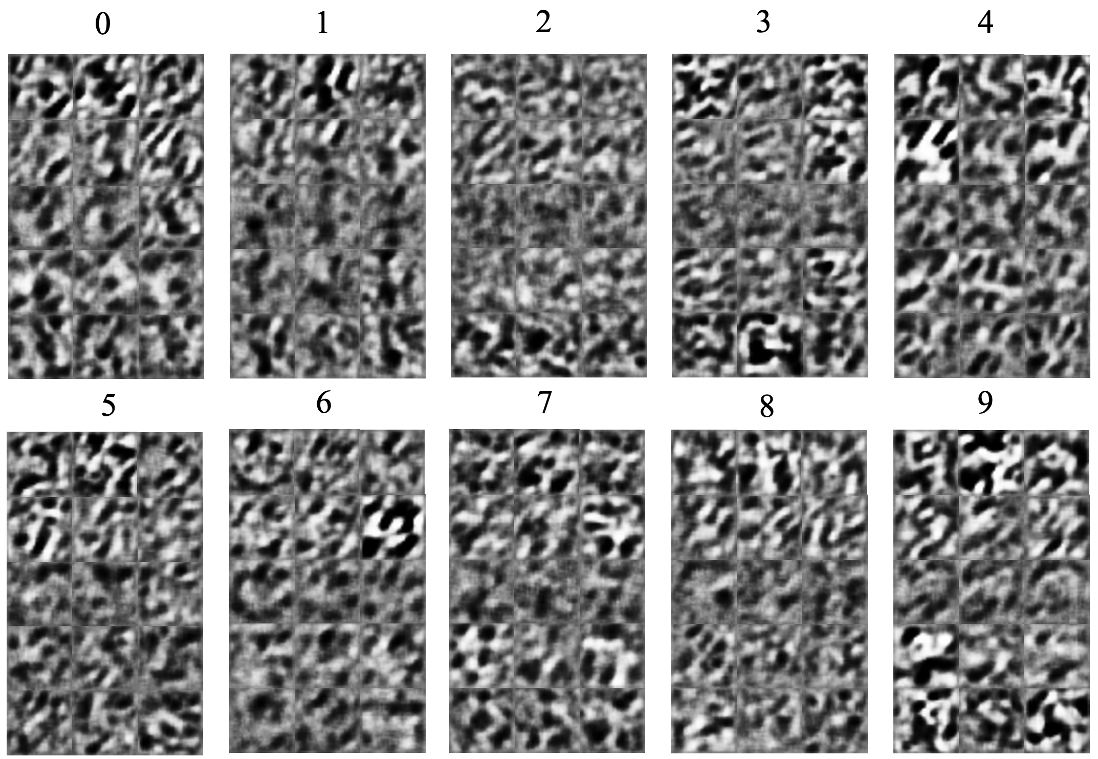
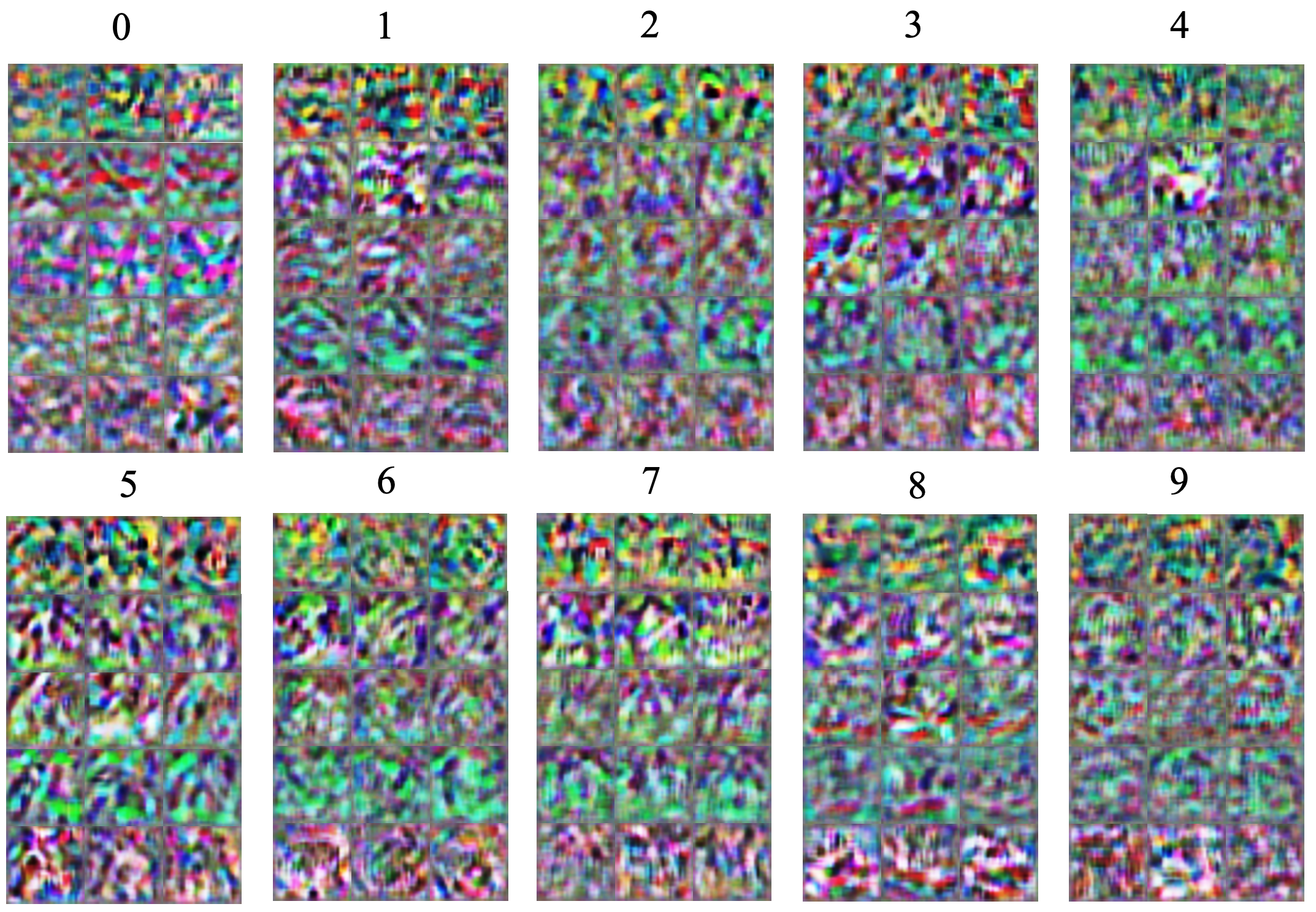
We conduct data visualization for the synthetic data of our proposed Co-Boosting on the MNIST and CIFAR-10 datasets in Fig. 4 and Fig. 5, where digits 0 to 9 represent 10 different classes. There are a total of five rows corresponding to images generated at the 100th, 200th, 300th, 400th, and 500th global model training epochs. For each epoch, we randomly select 3 images for display. From the figures, it can be observed that the generated data does not hold significant practical value to the human eye. However, it is sufficient for machine learning models to learn a robust classifier.