Epstein Surfaces, $W$-Volume, and the Osgood-Stowe Differential

Abstract

In a seminal paper, Epstein introduced the theory of what are now called Epstein surfaces, which construct surfaces in ${{\mathbb{H}}^{3}}$ associated to a conformal metric on a domain in $\widehat{{\mathbb{C}}}$. More recently, these surfaces have been used by Krasnov-Schlenker to define the $W$-volume and renormalized volume associated with a convex co-compact hyperbolic 3-manifold. In this paper, we describe an alternate construction of Epstein surfaces using the Osgood-Stowe differential, a generalization of the Schwarzian derivative. Krasnov-Schlenker showed that the metric and shape operator of a surface in hyperbolic space is naturally dual to a conformal metric and shape operator on a projective structure via the hyperbolic Gauss map. We show that this projective shape operator can be derived from the Osgood-Stowe differential. Using this approach, we provide a self-contained development of Epstein surfaces, $W$-volume, and renormalized volume. We further prove a number of new results, including a generalization of Epstein’s univalence criterion, a variational formula for W-volume in terms of the Osgood-Stowe differential, and use $W$-volume to relate the length of the bending lamination of the convex core to the norm of the Schwarzian derivative.

1 Introduction

In [Eps4] Epstein gave a beautiful construction of a surface in ${{\mathbb{H}}^{3}}$ associated to a conformal metric on a domain $\Omega\subset\widehat{{\mathbb{C}}}=\partial{{\mathbb{H}}^{3}}$. This construction has been very influential. For example, in a pair of follow-up papers [Eps2, Eps3] Epstein used these surface to give a new univalence condition for conformal maps of the disk. More recently, these surfaces have been used to define the renormalized volume of a convex co-compact hyperbolic 3-manifold.

In Epstein’s original construction the surface was described as an envelope of horospheres. Epstein gave parametric equations for these Epstein surfaces and then from this parameterization was able to calculate the first and second fundamental forms of the surface. Here will we give an alternate construction of Epstein’s surfaces. In our approach rather than calculate the first and second fundamental forms from a parameterization of the surface, motivated by work of Krasnov-Schlenker, we describe them as “dual” to certain forms on the domain $\Omega$ (or more generally on a complex projective structure). These forms satisfy the classical surface equations of Gauss and Codazzi and therefore are realized as surfaces in ${{\mathbb{H}}^{3}}$.

The pair of forms on $\Omega$ are a conformal metric and the metric’s Osgood-Stowe differential (see [OS2]), which plays the role of the second fundamental form. The Osgood-Stowe differential generalizes the Schwarzian quadratic differential - if the conformal metric is the hyperbolic metric then the Osgood-Stowe differential is exactly the Schwarzian differential of the uniformizing map.

After developing the theory of Epstein surfaces we then revisit Epstein’s univalence criteria, giving new proofs that also generalize Epstein’s results.

In recent work motivated from physics, Krasnov-Shlenker [KS1] introduced the notion of $W$-volume for convex, compact hyperbolic 3-manifolds. Via Epstein surfaces, $W$-volume can be interpreted as a smooth functional on the space of conformal metrics on the boundary of conformally compact but infinite volume hyperbolic 3-manifold. In [KS1] and [Sch1] they prove many fundamental properties of W-volume and the related functional, renormalized volume $V_{R}$. These include a variational formula for $W$-volume and a new proof that $dV_{R}$ is the Schwarzian derivative of the uniformization map for the conformal boundary. Our approach to Epstein surfaces naturally gives a new variational formula for $W$-volume in terms of the Osgood-Stowe differential from which the properties of $W$-volume developed by Krasnov-Schlenker can easily be extended. In particular, we give a new inequality bounding the $L^{2}$-norm of the Schwarzian derivative of a projective structure by the length of its associated bending lamination.

While much of what we do here is known, our approach is elementary and self contained. In particular, we give complete proofs of the main results in [Eps2, Eps3, Eps4] and [KS1] along with several extensions and new results. We also mention recent work of Quinn who has developed many of these ideas in higher dimensions (see [Qui]).

Acknowledgements: We would like to thank Mladen Bestvina, Curt McMullen, Keaton Quinn, Franco Vargas-Pallete, Jean-Marc Schlenker and Rich Schwartz for useful comments and suggestions.

2 Results

We now describe the main results of the paper. As well as these, we will also use our approach to give elementary proofs of many of the fundamental results on Epstein surfaces and W-volume. Our hope is that this will give a self-contained description to both subjects as well as a unifying approach.

2.1 Duality, Osgood-Stowe Differential

If $S$ is a surface embedded in a hyperbolic 3-manifold then the induced metric on $g$ and shape operator $B\colon TS\to TS$ satisfy the Gauss-Codazzi equations. Conversely, if $g$ is metric and $B$ a bundle endomorpshism that satisfy the Gauss-Codazzi equations then, by a classical theorem of Bonnet, they are the metric and shape operator of a surface in a hyperbolic 3-manifold. Here we will develop a parallel theory for conformal metrics on complex projective structures where our replacement for the shape operator will be a tensor developed by Osgood-Stowe in [OS2]. Moreover we will see that there is a duality between these two theories.

If $g$ is Riemannian metric then any conformally equivalent metric can be written as $e^{2\phi}g$ where $\phi$ is a real valued function. The Osgood-Stowe tensor is the traceless part of the Hessian of $\phi$ and can be considered a measure of the difference between the two metrics. While this is defined in all dimensions here we will restrict to the case of conformal metrics on a Riemann surface where the tensor can be naturally identified with a quadratic differential on the surface. One very concrete example is when $\Omega$ is a hyperbolic domain in $\mathbb{C}$. Then the Osgood-Stowe tensor between the hyperbolic metric on $\Omega$ and the Euclidean metric on $\mathbb{C}$ gives the Schwarzian derivative of the conformal map uniformizing $\Omega$. A slight variation of these ideas gives a version of the Osgood-Stowe tensor for any conformal metric on a complex projective structure on a surface.

We will see that this tensor plays a role similar to that of the second fundamental form of a surface embedded in a space. Namely, if $g$ is a conformal metric on a projective structure $\Sigma$ then we can define a projective shape operator $B(\Sigma,g)$ via the Osgood-Stowe tensor. Then the projective Gauss-Codazzi equations are

$$\begin{array}[]{ll}d^{\nabla}B=0&\qquad\mbox{(Codazzi)}\\ \operatorname{Tr}(B)=-2K(g)&\qquad\mbox{(Gauss)}\end{array}$$

where $K(g)$ is the Gaussian curvature of $g$, $\nabla$ the Riemannian connection for $g$, and $d^{\nabla}$ is defined on an endomorphism $A:TS\rightarrow TS$ by

$$d^{\nabla}A(X,Y)=\nabla_{X}(A(Y))-\nabla_{Y}(A(X))-A([X,Y]).$$

We prove:

Theorem 2.1

A pair $(g,B)$ on a surface $S$ satisfies the projective Gauss-Codazzi equations if and only if there exists a projective structure $\Sigma$ on $S$ such that $g$ is a conformal metric on $\Sigma$ and $B=B(\Sigma,g)$. Furthermore $\Sigma$ is unique.

Before describing the duality we review the classical theory of immersed surfaces. Let $M$ be a hyperbolic 3-manifold with Levi-Civita connection $\overline{\nabla}$ and $S$ an immersed surface in $M$ with induced metric $g$. Then the shape operator of $S$ is the endomorphism $B:TS\rightarrow TS$ of the tangent bundle $TS$ of $S$ defined by $B(v)=\overline{\nabla}_{v}n$ where $n$ is a choice of unit normal vector field to $S$. For $S$ the boundary of a manifold $N$ our convention will be to let $n$ be the outward normal.

The shape operator $B$ is symmetric with respect to the metric $g$ and its eigenvalues at a point are the principal curvatures. The pair $(g,B)$ satisfy the Gauss-Codazzi equations in ${{\mathbb{H}}^{3}}$ given by

$$\begin{array}[]{ll}d^{\nabla}B=0&\qquad\mbox{(Codazzi)}\\ \det(B)=K(g)+1.&\qquad\mbox{(Gauss)}\end{array}$$

A classical result due to Bonnet, referred to as the fundamental theorem for immersed surfaces, gives the following converse.

Theorem 2.2 (Bonnet)

If $S$ is simply connected and the pair $(g,B)$ satisfy the Gauss-Codazzi equations in ${{\mathbb{H}}^{3}}$ then there is an immersion

$$f\colon S\to{{\mathbb{H}}^{3}}$$

with $g=f^{*}g_{{\mathbb{H}}^{3}}$ and shape operator $B$. Furthermore $f$ is unique up to post-composition with isometries of ${{\mathbb{H}}^{3}}$.

In [KS1] Krasnov-Schlenker show that the image of an immersed surface in ${{\mathbb{H}}^{3}}$ under the hyperbolic Gauss map to $\hat{\mathbb{C}}$ defines a pair $(\hat{g},\hat{B})$ which satisfy the projective Gauss-Codazzi equations. There is a natural duality of pairs $(g,B)\longleftrightarrow(\hat{g},\hat{B})$ which can be defined by

$$\hat{g}(X,({\operatorname{Id}}+\hat{B})Y)=2g(({\operatorname{Id}}+B)X,Y)\qquad({\operatorname{Id}}+B)({\operatorname{Id}}+\hat{B})=2{\operatorname{Id}}.$$

Equivalently we can write the duality by

$$\hat{g}(X,Y)=g(({\operatorname{Id}}+B)X,({\operatorname{Id}}+B)Y)\qquad\hat{B}=({\operatorname{Id}}+B)^{-1}({\operatorname{Id}}-B)$$

and

$$g(X,Y)=\frac{1}{4}\hat{g}(({\operatorname{Id}}+\hat{B})X,({\operatorname{Id}}+\hat{B})Y)\qquad B=({\operatorname{Id}}+\hat{B})^{-1}({\operatorname{Id}}-\hat{B}).$$

We have:

Theorem 2.3 (see also Schlenker, [Sch2])

Let $(g,B)$ and $\left(\hat{g},\hat{B}\right)$ be dual. Then $(g,B)$ satisfies the Gauss-Codazzi equations in ${{\mathbb{H}}^{3}}$ if and only if $\left(\hat{g},\hat{B}\right)$ satisfy the projective Gauss-Codazzi equations.

Observe that a local diffeomorpshism $f\colon S\to\widehat{{\mathbb{C}}}$ defines a projective structure $\Sigma=(S,f)$ on $S$. If $\hat{g}$ is a conformal metric on $\Sigma$ with $\hat{B}=B(\Sigma,\hat{g})$ the projective shape operator then by the theorem of Bonnet there is an immersion $f_{0}\colon S\to{{\mathbb{H}}^{3}}$ with metric and shape operator $(g,B)$ that is dual to $(\hat{g},\hat{B})$. On the other hand with the exact same setup Epstein ([Eps4]) described a map $f_{\operatorname{ep}}\colon S\to{{\mathbb{H}}^{3}}$ as an envelope of horospheres. We show that these surfaces are the same:

Theorem 2.4

Let $\Sigma=(S,f)$ be a simply connected projective structure and $\hat{g}$ a conformal metric on $\Sigma$. Then $f_{0}=f_{{\operatorname{ep}}}$.

2.2 Univalence criteria

In a pair of papers (see [Eps2, Eps3]) used (what are now called) Epstein surfaces to give new univalence criteria for conformal maps of the disk to $\widehat{{\mathbb{C}}}$ as well as a criterion for when the conformal map extended to a quasiconformal homeomorphism of the Riemann sphere. These criteria generalized Nehari’s univalence condition (see [Neh]) as well as the Ahlfors-Weill Extension Theorem (see [AW]). Osgood-Stowe in [OS1] and subsequently Chuaqui in [Chu], reinterpreted Epstein’s univalence criteria in terms of the Osgood-Stowe differential and proved generalizations. Using a different approach, we give the following further generalization of Epstein and those of Osgood-Stowe and Chuaqui. Our results are most conveniently stated in terms of the Schwarzian tensor $Q(\Sigma,g)$ which is a complexification of the Osgood-Stowe tensor.

Theorem 2.5

Let $\hat{g}$ be a complete metric on $\Delta$, $f\colon\Delta\to\widehat{{\mathbb{C}}}$ a locally univalent map and $\Sigma=(\Delta,f)$ the associated projective structure on $\Delta$.

1. If

   $$\|Q(\Sigma,\hat{g})\|\leq-\frac{1}{4}K(\hat{g})$$

   then $f$ is univalent and extends continuously to $\overline{\Delta}$.

2. If

   $$\|Q(\Sigma,\hat{g})\|<-\frac{1}{4}K(\hat{g})$$

   then $f$ extends to a homeomorphism of $\hat{\mathbb{C}}$.

3. If $K(\hat{g})<0$ and

   $$-\frac{4\|Q(\Sigma,\hat{g})\|}{K(\hat{g})}\leq k<1.$$

   Then $f$ extends to a quasiconformal homeomorphism with beltrami differential $\|\mu\|_{\infty}\leq k$.

Setting $\hat{g}=g_{{\mathbb{H}}^{2}}$ we observe that the univalence criterion above gives Nehari’s univalence criterion that a locally univalent map $f:\Delta\rightarrow\hat{\mathbb{C}}$ is univalent if the Schwarzian $\|Sf\|_{\infty}\leq\frac{1}{2}$ (see [Neh]). The quasiconformal criterion similarly generalizes the Ahlfors-Weill Extension Theorem which proves that if $\|Sf\|_{\infty}<\frac{k}{2}<\frac{1}{2}$ then $f$ extends to a $(1+k)/(1-k)$-quasiconformal homeomorphism (see [AW]).

2.3 $W$-volume

If $\bar{X}$ is a compact, hyperbolizable 3-manifold with boundary then given any metric $\hat{g}$ on the $\partial\bar{X}$ there is a complete hyperbolic structure on $X$ (the interior of $\bar{X}$) that is conformally compactified by a conformal structure in the conformal class of $\hat{g}$. The conformal boundary of this structure also determines a projective structure on $\partial\bar{X}$ so there is a projective shape operator $\hat{B}=B(\partial\bar{X},\hat{g})$. The dual pair $(g,B)$ will determine a surface in $X$. For now we will assume that the surface is embedded and therefore bounds a compact submanifold $N\subset X$. Then the W-volume of $N$ is defined by

$$W(N)=V(N)-\frac{1}{2}\int_{\partial N}HdA$$

where $H$ is the mean curvature of the boundary $\partial N$. The $W$-volume can be considered as a functional on the space of smooth metric on $\partial\bar{X}$ (again here we are ignoring some technicalities that arise when the surface determined by $(g,B)$ is not embedded). If $\nu$ is a variation of $\hat{g}$ the we have a formula for the variation $dW(\nu)$ which will be in terms of Schwarzian tensor $Q(\partial\bar{X},\hat{g})$ for the projective boundary, the Beltrami differential $\mu(\nu)$ which describes the infinitesimal change of conformal structure induced by $\nu$, and $dK(\nu)$, the infinitesimal change in curvature induced by $\nu$.

Theorem 2.6

The variational formula for $W$ is given by

$$dW(v)=\frac{1}{4}\int_{\partial\bar{X}}dK(v)dA_{\hat{g}}-2\operatorname{Re}\int_{\partial\bar{X}}Q(\partial\bar{X},\hat{g})\cdot\mu(v).$$

For two metrics in the same conformal class the underlying hyperbolic 3-manifolds will be isometric. In each conformal class there is a unique hyperbolic metric so by restricting to these metrics we get a function on $\mathcal{CC}(X)$ the space of convex co-compact hyperbolic metrics on $X$. This is the renormalized volume, denoted $V_{R}$. Then our variational formula reduces to the well known variational formula for $V_{R}$ first proved by Takhtajan-Zograf and Takhtajan-Teo (see [TZ], [TT]) in their work on the Liouville action. A proof of the variational formula for $V_{R}$ using methods similar to those in this paper was given by Krasnov-Schlenker in [KS1].

Theorem 2.7 ([TZ], [TT], [KS1])

The variation of $V_{R}$ on $\mathcal{CC}(X)$ is given by

$$(dV_{R})(v)=\operatorname{Re}\int_{\partial\bar{X}}Q(X,\hat{g})\cdot\mu(v).$$

2.4 $W$-volume for pairs, projective structures

Given two conformal metrics $g,h$ on $\partial\bar{X}$ it is natural to define the $W$-volume of the pair by

$$W(g,h)=W(h)-W(g).$$

One motivation for defining this is that it can be extended to projective structures. In particular if ${\cal G}(\Sigma)$ is the space of smooth conformal metrics on a projective structure $\Sigma$ on a closed surface $S$ of genus $g\geq 2$ then for $g,h\in{\cal G}(\Sigma)$ we define $W(g,h)$. This $W$-volume for pairs agrees with the $W$-volume for pairs on $\partial\bar{X}$ by taking $\Sigma=\Sigma_{X}$.

In [KS1], Krasnov-Schlenker proved a monotonicity property of $W$-volume, that if $g\leq h$ pointwise and both have non-positive curvature, then $W(g)\leq W(h)$ or equivalently that $W(g,h)\geq 0$. We generalize this monotonicity property as well as the scaling property of $W$-volume in the below theorem. If $g$ is a smooth metric we define the curvature form by $\Omega_{g}=K(g)dA_{g}$.

Theorem 2.8

Let $g,h\in{\cal G}(\Sigma)$ with $h=e^{2u}g$. Then

$$W(g,h)=-\frac{1}{4}\int_{\Sigma}u\left(\Omega_{g}+\Omega_{h}\right)=-\frac{1}{8}(\Omega_{g}+\Omega_{h})\left(\log\left(h/g\right)\right).$$

In particular for $g\leq h$ pointwise and both non-positively curved, then $W(g,h)\geq 0$.

In [KS1], Krasnov-Schlenker proved that in the quasifuchsian case, the hyperbolic metric had maximal $W$-volume over all conformal metrics with the same area. We prove the following generalization which gives a new proof of the original maximality property of Krasnov-Schlenker.

Theorem 2.9

Let $g,h\in{\cal G}(\Sigma)$ with $h=e^{2u}g$ such that $g,h$ have the same area and $g$ has constant curvature. Then

$$W(g,h)\leq-\frac{1}{4}\|\nabla u\|_{2}^{2}$$

where $\nabla$ is the gradient of $g$. In particular $h=g$ is the unique maximum.

2.5 Schwarzian derivatives and bending laminations

Thurston showed that complex projective structures on a surface are parameterized by pairs $(g,\lambda)$ where $g$ is a hyperbolic metric and $\lambda$ is a measured lamination. When $\Sigma$ is the conformal boundary of a hyperbolic 3-manifold then $g$ is the metric on the boundary convex core facing $\Sigma$ and $\lambda$ is the bending lamination (see [KT] for details). Also associated to the projective structure is the Schwarzian quadratic differential $\phi_{\Sigma}$. Using $W$-volume, given a projective structure $\Sigma$ we show the following surprising relation between the norms $\|\phi_{\Sigma}\|_{2},\|\phi_{\Sigma}\|_{\infty},$ and the length $L(\lambda_{\Sigma})$ of the bending lamination $\lambda_{\Sigma}$ of $\Sigma$ given by its Thurston parametrization.

Theorem 2.10

Let $\Sigma$ be a projective structure with Thurston parameterization $\left(Y_{\Sigma},\lambda_{\Sigma}\right)$. Then

$$\|\phi_{\Sigma}\|_{2}\leq(1+\|\phi_{\Sigma}\|_{\infty})\sqrt{L(\lambda_{\Sigma})}.$$

By Nehari (see [Neh]) if $\Sigma$ is the quotient of a domain in $\widehat{{\mathbb{C}}}$ then $\|\phi_{\Sigma}\|_{\infty}\leq 3/2$. Therefore we obtain the following corollary.

Corollary 2.11

Let $\Sigma$ be the quotient of a domain in $\widehat{{\mathbb{C}}}$. Then

$$\|\phi_{\Sigma}\|_{2}\leq\frac{5}{2}\sqrt{L(\lambda_{\Sigma})}.$$

For example, this situation arises when $\Sigma$ is an incompressible boundary component of a convex co-compact hyperbolic 3-manifold.

3 Linear algebra

As we will be working with conformal metrics on Riemann surfaces, it will be natural to describe tensors and forms in terms of the underlying complex structure even when the objects are $\mathbb{R}$-linear. We now describe the elementary linear algebra needed to do this.

Let $J$ be the standard (almost) complex structure on $\mathbb{R}^{2}$. If ${\partial_{x}}$ and ${\partial_{y}}$ are the standard basis of $\mathbb{R}^{2}$ then

$${\partial_{z}}=\frac{1}{2}\left({\partial_{x}}-i{\partial_{y}}\right)\mbox{ and }{\partial_{\overline{z}}}=\frac{1}{2}\left({\partial_{x}}+i{\partial_{y}}\right)$$

are a basis of $\mathbb{R}^{2}\otimes\mathbb{C}$. If $dx$ and $dy$ are the dual basis (with respect to $\mathbb{R}$) of $\mathbb{R}^{2}$ then

$$dz=dx+idy\mbox{ and }d{\overline{z}}=dx-idy$$

are the dual basis (with respect to $\mathbb{C}$) to ${\partial_{z}}$ and ${\partial_{\overline{z}}}$. Note that both $dz$ and $d{\overline{z}}$ are $\mathbb{C}$-linear on $\mathbb{R}^{2}\otimes\mathbb{C}$ but when restricted to $\mathbb{R}^{2}$, $dz$ is $\mathbb{C}$-linear with respect to the complex structure $\left(\mathbb{R}^{2},J\right)$ and $d{\overline{z}}$ is $\mathbb{C}$-anti-linear. It will be useful to write objects in complex coordinates (even if they are not $\mathbb{C}$-linear with respect to $\left(\mathbb{R}^{2},J\right)$).

The following “dot” notation will be useful. Let $T$ be an $\mathbb{R}$-linear 2-tensor and $B$ an $\mathbb{R}$-linear map. Then define the 2-tensor $T\cdot B$ by

$$T\cdot B(X,Y)=T(BX,Y).$$

If we fix a metric on $g$ on $\mathbb{R}^{2}$ we can use this to change the type of a tensor: If we are given either $T$ or $B$ the formula

$$T=g\cdot B$$

determines the other.

We can then define the trace of $T$ by $\operatorname{Tr}_{g}(T)=\operatorname{Tr}(B)$. As $B$ depends on the metric so will $\operatorname{Tr}_{g}(T)$. The metric $g$ is conformal (with respect to the complex structure $(\mathbb{R}^{2},J)$) if $J$ is an isometry. This is equivalent to being a multiple of the usual Euclidean metric ${g_{\rm euc}}$. We note that $\operatorname{Tr}_{g_{\rm euc}}(T)=0$ if and only $\operatorname{Tr}_{g}(T)=0$ for all conformal metrics.

Both 2-tensors on $\mathbb{R}^{2}$ and linear maps of $\mathbb{R}^{2}$ to itself have unique $\mathbb{C}$-linear extensions to $\mathbb{R}^{2}\otimes\mathbb{C}$. If the $\mathbb{R}$-linear versions of $T$, $B$ and $g$ satisfy the equation $T=g\cdot B$ then so will their $\mathbb{C}$-linear extensions. The change of basis from complex coordinates to real coordinates is given by the matrix

$${\mathcal{A}}=\left(\begin{array}[]{cc}1/2&1/2\\ -i/2&i/2\end{array}\right)$$

so if $T$ is written as a matrix in the basis $\{{\partial_{x}},{\partial_{y}}\}$ then its matrix representation in the complex basis $\{{\partial_{z}},{\partial_{\overline{z}}}\}$ is

$${\mathcal{A}}^{t}T{\mathcal{A}}.$$

For example, the usual Euclidean inner product ${g_{\rm euc}}$ on $\mathbb{R}^{2}$ is given by the identity matrix in the real basis so its $\mathbb{C}$-linear extension in the complex basis is given by

$${\mathcal{A}}^{t}{\operatorname{Id}}{\mathcal{A}}=\left(\begin{array}[]{cc}0&1/2\\ 1/2&0\end{array}\right).$$

In particular ${g_{\rm euc}}({\partial_{z}},{\partial_{z}})={g_{\rm euc}}({\partial_{\overline{z}}},{\partial_{\overline{z}}})=0$ while ${g_{\rm euc}}({\partial_{z}},{\partial_{\overline{z}}})={g_{\rm euc}}({\partial_{\overline{z}}},{\partial_{z}})=1/2$.

More generally if

$$T=\left(\begin{array}[]{cc}x+y&r+s\\ r-s&x-y\end{array}\right)$$

then

$${\mathcal{A}}^{t}T{\mathcal{A}}=\frac{1}{2}\cdot\left(\begin{array}[]{cc}y-ir&x+is\\ x-is&y+ir\end{array}\right).$$

This gives us the following lemma.

Lemma 3.1

Let $T$ be a $\mathbb{C}$-bilinear tensor on $\mathbb{R}^{2}\otimes\mathbb{C}$ that is real on $\mathbb{R}^{2}\otimes\mathbb{R}$ and $g$ a conformal metric. If $T$ is symmetric and traceless over $\mathbb{R}^{2}\otimes\mathbb{R}$ then

$$T=Qdz^{2}+\bar{Q}d{\overline{z}}^{2}$$

where

$$Q=\frac{1}{2}\cdot(T({\partial_{x}},{\partial_{x}})-iT({\partial_{x}},{\partial_{y}})).$$

We also get formulas for the trace.

Lemma 3.2

Let $T$ be a $\mathbb{C}$-bilinear tensor on $\mathbb{R}^{2}\otimes\mathbb{C}$ that is real on $\mathbb{R}^{2}\otimes\mathbb{R}$ and $g$ a conformal metric. Then

$$\operatorname{Tr}_{g}(T)=\frac{T({\partial_{z}},{\partial_{\overline{z}}})+T({\partial_{\overline{z}}},{\partial_{z}})}{g({\partial_{z}},{\partial_{\overline{z}}})}$$

and if $T$ is symmetric

$$\operatorname{Tr}_{g}(T)=2\operatorname{Re}\frac{T({\partial_{z}},{\partial_{\overline{z}}})}{g({\partial_{z}},{\partial_{\overline{z}}})}.$$

Given a conformal metric $g=\lambda\cdot{g_{\rm euc}}$ the area form is the alternating 2-tensor given by the matrix

$$\left(\begin{array}[]{cc}0&\lambda\\ -\lambda&0\end{array}\right)$$

in the basis $\{{\partial_{x}},{\partial_{y}}\}$ for $\mathbb{R}^{2}$. In complex coordinates we then have:

Lemma 3.3

Let $g$ be a conformal metric. Then the area form for $g$ is

$$dA_{g}=2g({\partial_{z}},{\partial_{\overline{z}}})dx\wedge dy=-ig({\partial_{z}},{\partial_{\overline{z}}})dz\wedge d{\overline{z}}.$$

3.1 Pairing

We define a pairing between $T$ an $B$ by

$$\langle T,B\rangle_{g}=\frac{1}{2}\operatorname{Tr}_{g}(T\cdot B)dA_{g}$$

where $g$ is any conformal metric with respect to $J$. It is clear that the definition is independent of the conformal metric $g$ chosen and the pairing is $\mathbb{R}$-linear in both $T$ and $B$. We will drop the subscript when the conformal class is obvious. Choosing $g=g_{euc}$ by Lemma 3.2

$$\langle T,B\rangle=\left(T\left({\partial_{z}},B{\partial_{\overline{z}}}\right)+T\left({\partial_{\overline{z}}},B{\partial_{z}}\right)\right)dx\wedge dy.$$

Our normalization is chosen such that

$$\left\langle dz^{2},{\partial_{z}}\otimes d{\overline{z}}\right\rangle=dx\wedge dy.$$

This pairing is the usual pairing between quadratic differentials and Beltrami differentials from Teichmüller theory. The following is an immediate consequence of the definition.

Lemma 3.4

Let $g$ be a conformal metric and $A,B$ linear maps. Then

$$\langle g\cdot A,B\rangle=\langle g\cdot B,A\rangle=\frac{1}{2}\operatorname{Tr}(AB)dA_{g}.$$

Furthermore if $T$ is symmetric and traceless then

$$\langle T,B\rangle=\langle T,B_{0}\rangle.$$

Proof: As $(g\cdot A)\cdot B=g\cdot(AB)$ and $\operatorname{Tr}_{g}(g\cdot M)=\operatorname{Tr}(M)$ we have

$$\langle g\cdot A,B\rangle=\frac{1}{2}\operatorname{Tr}_{g}((g\cdot A)\cdot B)dA_{g}=\frac{1}{2}\operatorname{Tr}_{g}(g\cdot(AB))dA_{g}=\frac{1}{2}\operatorname{Tr}(AB)dA_{g}.$$

The first result follows by symmetry and the second by orthogonality.$\Box$

3.2 Variations

If $X_{t}$ is a one-parameter family of tensors then its time zero derivative $\delta X$ is a tensor of the same type. Then $\delta X$ is a variation of $X$. Often a variation of $X$ will induce a variation of another tensor and we will use the $\delta$-notation to refer to the variation of this other tensor. For example, if $P$ is a linear isomorphism and $\hat{P}$ is its inverse the variation $\delta P$ of $P$ will induce a variation $\delta\hat{P}$ of $\hat{P}$ and by the product rule we have

$$\delta P\hat{P}+P\delta\hat{P}=0.$$

We now show that the pairing for two metrics satisfy a variational property.

Lemma 3.5

Let $g,\hat{g}$ be metrics on $\mathbb{R}^{2}$ related by $\hat{g}=P^{*}g$ where $P$ is symmetric with respect to $g$. Equivalently $g=\hat{P}^{*}\hat{g}$ where $\hat{P}$ is symmetric with respect to $\hat{g}$ and $P\hat{P}={\operatorname{Id}}$. Then under a smooth variation of $(g,P)$

$$\langle\hat{g},\delta\hat{P}\rangle_{\hat{g}}+\langle\delta\hat{g},\hat{P}_{0}\rangle_{\hat{g}}=-\operatorname{sgn}(\det(P))\left(\langle g,\delta P\rangle_{g}+\langle\delta g,P_{0}\rangle_{g}\right)$$

where $P_{0},\hat{P}_{0}$ are the traceless part of $P,\hat{P}$ respectively.

Proof: We differentiate $P\hat{P}={\operatorname{Id}}$. This gives

$$\delta\hat{P}=-P^{-1}\delta PP^{-1}.$$

By the Cayley-Hamilton Theorem for linear maps on $\mathbb{R}^{2}$

$$P^{2}-\operatorname{Tr}(P)P+\det(P){\operatorname{Id}}=0.$$

Multiplying by $P^{-1}$ we get

$$P=2P_{0}+\det(P)P^{-1}\qquad\det(P)(P^{-1})_{0}=-P_{0}\qquad{\operatorname{Id}}=2P_{0}P^{-1}+\det(P)P^{-2}.$$

As $\hat{P}=P^{-1}$ then

$$\hat{P}_{0}=-\frac{P_{0}}{\det(P)}.$$

As $\hat{g}=P^{*}g$ and $P$ is symmetric with respect to $g$, then $\hat{g}=g\cdot P^{2}$. We define linear maps $\eta,\hat{\eta}$ by $\delta g=g\cdot\eta,\delta\hat{g}=\hat{g}\cdot\hat{\eta}$. Then differentiating $\hat{g}=g\cdot P^{2}$ gives

$$\delta\hat{g}=\delta g\cdot P^{2}+g\cdot(\delta PP+P\delta P)=g\cdot(\eta P^{2}+\delta PP+P\delta P).$$

As $\delta\hat{g}=\hat{g}\cdot\hat{\eta}=g\cdot(P^{2}\hat{\eta})$ we get

$$\hat{\eta}=P^{-2}\eta P^{2}+P^{-2}\delta PP+P^{-1}\delta P.$$

By definition of the pairing $\langle\ ,\ \rangle_{\hat{g}}$

$$\langle\hat{g},\delta\hat{P}\rangle_{\hat{g}}+\langle\delta\hat{g},\hat{P}_{0}\rangle_{\hat{g}}=\frac{1}{2}\operatorname{Tr}_{\hat{g}}(\hat{g}\cdot\delta\hat{P}+\delta\hat{g}\cdot\hat{P}_{0})dA_{\hat{g}}=\frac{1}{2}\operatorname{Tr}(\delta\hat{P}+\hat{\eta}\hat{P}_{0})dA_{\hat{g}}.$$

By definition of the area form we have

$$dA_{\hat{g}}=|\det(P)|dA_{g}=\operatorname{sgn}(\det(P))\det(P)dA_{g}.$$

Applying $\operatorname{Tr}(XY)=\operatorname{Tr}(YX)$ and the Cayley-Hamilton Theorem

$$\operatorname{Tr}(\delta\hat{P}+\hat{\eta}\hat{P}_{0})dA_{\hat{g}} = -\operatorname{sgn}(\det(P))\operatorname{Tr}\left(\delta P\left(2P_{0}P^{-1}+\det(P)P^{-2}\right)+\eta P_{0}\right)dA_{g}$$

$$= -\operatorname{sgn}(\det(P))\operatorname{Tr}(\delta P+\eta P_{0})dA_{g}.$$

The result then follows.$\Box$

3.3 Metric variations and the strain tensor

If $g$ is a metric in the conformal class of the usual complex structure on $\mathbb{R}^{2}$ and $\delta g$ is a variation of $g$ then we define the linear map $\eta\colon\mathbb{R}^{2}\to\mathbb{R}^{2}$ by

$$\delta g=2g\cdot\eta.$$

A simple calculation shows that the variation of the area form $dA_{g}$ satisfies

$$\delta(dA_{g})=\operatorname{Tr}(\eta)dA_{g}.$$

The traceless part $\eta_{0}$ of $\eta$ is the strain of the variation and it measures the change of conformal structure. If we complexify, by Lemma 3.1 we see that

$$\eta_{0}=\nu{\partial_{z}}\otimes d{\overline{z}}+\overline{\nu}{\partial_{\overline{z}}}\otimes dz$$

for some $\nu\in\mathbb{C}$. We then define the Betrami differential for the metric variation by $\mu(\delta g)=\nu{\partial_{z}}\otimes d{\overline{z}}$.

3.4 Linear algebra on the complexified tangent bundle

We can extend this discussion to the tangent bundle $TX$ of a Riemann surface $X$. Namely, the one complex dimensional subspaces spanned by ${\partial_{z}}$ and ${\partial_{\overline{z}}}$ are invariant under automorphisms of the almost complex structure $\left(\mathbb{R}^{2},J\right)$. In particular, the bundle $TX\otimes\mathbb{C}$ has a decomposition into complex line bundles $T^{1,0}X$ and $T^{0,1}X$ where the former is spanned by ${\partial_{z}}$ and the later by ${\partial_{\overline{z}}}$. We will only use when $X$ is a domain in $\mathbb{C}$ where using complex coordinates will greatly simplify some computations.

For example if $f\colon X\to\mathbb{R}$ is a smooth function then we can take the usual differential $df$ which is $\mathbb{R}$-valued 1-form (a section of the co-tangent bundle) and extend it to a section of the dual bundle (over $\mathbb{C}$) of $TX\otimes\mathbb{C}$ by declaring it to be $\mathbb{C}$-linear. With this extension we have that

$$df=f_{z}dz+f_{\overline{z}}d{\overline{z}}$$

is a section of the dual bundle of $TX\otimes\mathbb{C}$ that when restricted to $TX\cong TX\otimes\mathbb{R}$ this section is $\mathbb{R}$-valued and is the usual differential of $f$.

Let $g_{\phi}(,)=e^{2\phi}\langle,\rangle$ be a conformal metric on $X$ where $\langle,\rangle$ is the usual Euclidean inner product on $\mathbb{R}^{2}$. Let $\nabla^{\phi}$ be the Levi-Civita connection for $g_{\phi}$. These both extend to $TX\otimes\mathbb{C}$ by declaring them to be $\mathbb{C}$-linear. Then in real coordinates the gradient is

$$\nabla^{\phi}f=e^{-2\phi}\left(f_{x}{\partial_{x}}+f_{y}{\partial_{y}}\right).$$

Using the matrix ${\mathcal{A}}^{-1}$ to change to complex coordinates this becomes

$$\nabla^{\phi}f=2e^{-2\phi}\left(f_{\overline{z}}{\partial_{z}}+f_{z}{\partial_{\overline{z}}}\right)$$

which naturally is a section of $TX\otimes\mathbb{C}$. We have the following elementary calculations.

Proposition 3.6

Let $g_{\phi}=e^{2\phi}{g_{\rm euc}}$ with Levi-Civita connection $\nabla^{\phi}$. Then

• $\nabla^{\phi}_{X}Y=\nabla_{X}Y+X(\phi)Y+Y(\phi)X-{g_{\rm euc}}(X,Y)\nabla\phi$;

• $\nabla^{\phi}_{{\partial_{z}}}{\partial_{z}}=2\phi_{z}{\partial_{z}}\qquad\nabla^{\phi}_{{\partial_{\overline{z}}}}{\partial_{\overline{z}}}=2\phi_{\overline{z}}{\partial_{\overline{z}}}\qquad\nabla^{\phi}_{{\partial_{z}}}{\partial_{\overline{z}}}=\nabla^{\phi}_{{\partial_{\overline{z}}}}{\partial_{z}}=0$;

• ${\operatorname{Hess}}f\left({\partial_{z}},{\partial_{z}}\right)=f_{zz}-2\phi_{z}f_{z}$.

Proof: We take the equation relating $\nabla^{\phi}$ and $\nabla$ as the definition of $\nabla^{\phi}$. One then checks that (1) it is a connection, (2) it is torsion free and (3) it is compatible with the metric $g_{\phi}$. Therefore it must be the Levi-Civita connection. Once we have verified this over $\mathbb{R}$ then the formula extends over $\mathbb{C}$.

The formulas for the covariant derivatives of ${\partial_{z}}$ and ${\partial_{\overline{z}}}$ then follow where we are using that ${g_{\rm euc}}\left({\partial_{z}},{\partial_{z}}\right)={g_{\rm euc}}\left({\partial_{\overline{z}}},{\partial_{\overline{z}}}\right)=0$ and ${g_{\rm euc}}\left({\partial_{z}},{\partial_{\overline{z}}}\right)={g_{\rm euc}}\left({\partial_{\overline{z}}},{\partial_{z}}\right)=1/2$.

To calculate the Hessian we use the formula

$${\operatorname{Hess}}f\left(X,Y\right)=g_{\phi}\left(\nabla^{\phi}_{X}\nabla^{\phi}f,Y\right).$$

To evaluate this when $X=Y={\partial_{z}}$ we only need to know the ${\partial_{\overline{z}}}$ term of $\nabla^{\phi}_{\partial_{z}}\nabla^{\phi}f$ and by the previous formulas this is

$$2e^{-2\phi}\left(-2\phi_{z}f_{z}+f_{zz}\right){\partial_{\overline{z}}}$$

and therefore

$${\operatorname{Hess}}f\left({\partial_{z}},{\partial_{z}}\right)=2e^{-2\phi}\left(-2\phi_{z}f_{z}+f_{zz}\right)g_{\phi}\left({\partial_{\overline{z}}},{\partial_{z}}\right)=f_{zz}-2\phi_{z}f_{z}.$$

$\Box$

4 The Osgood-Stowe differential

If $(M,g)$ is a Riemannian manifold and $f\colon M\to\mathbb{R}$ is a smooth function then the Osgood-Stowe differential ${\operatorname{\bf{OS}}}(f;g)$ is the traceless part of the 2-tensor

$${\operatorname{Hess}}f-df\otimes df.$$

If $M$ is Riemann surface and $g$ is a conformal metric then there is nice formula for ${\operatorname{\bf{OS}}}(f;g)$ in local coordinates.

Proposition 4.1

Let $\Omega$ be a domain in $\mathbb{C}$ and $g_{\phi}=e^{2\phi}{g_{\rm euc}}$ a conformal metric on $\Omega$. If $f\colon\Omega\to\mathbb{R}$ is a smooth function then

$${\operatorname{\bf{OS}}}(f;g_{\phi})=Q(f;g_{\phi})dz^{2}+\overline{Q(f;g_{\phi})}d{\overline{z}}^{2}$$

where

$$Q(f;g_{\phi})=f_{zz}-2\phi_{z}f_{z}-(f_{z})^{2}.$$

Proof: By Lemma 3.1, a symmetric traceless 2-tensor is of the form $Qdz^{2}+\overline{Q}d{\overline{z}}^{2}$ so to find ${\operatorname{\bf{OS}}}(f;g_{\phi})$ we only need to find ${\operatorname{\bf{OS}}}(f;g_{\phi})({\partial_{z}},{\partial_{z}})=Q$. By Proposition 3.6

$${\operatorname{Hess}}f({\partial_{z}},{\partial_{z}})=f_{zz}-2\phi_{z}f_{z}.$$

As

$$df\otimes df({\partial_{z}},{\partial_{z}})=(f_{z})^{2}$$

the proposition follows. $\Box$

Let $g_{0}$ and $g_{1}$ be conformal metrics on a Riemann surface $X$. Then $g_{1}=e^{2\phi}g_{0}$ for some real valued function $\phi$. We then define

$${\operatorname{\bf{OS}}}(g_{0},g_{1})={\operatorname{\bf{OS}}}(\phi;g_{0})\qquad\mbox{and}\qquad Q(g_{0},g_{1})=Q(\phi;g_{0}).$$

The tensor $Q$ is the Schwarzian tensor and has been studied in related papers by Dumas and Schlenker among others (see [Dum] and [Sch2]). The Schwarzian tensor is a quadratic differential, i.e. a section of the tensor product of the holomorphic cotangent bundle of $X$ with itself. Holomorphic quadratic differentials appear frequently in Teichmüller theory, and will play a special role here, but in general the Schwarzian tensor will not be holomorphic. We now state some basic properties of the Schwarzian tensor and include the proofs for completeness.

Proposition 4.2

The Osgood-Stowe differential satisfies

• ${\operatorname{\bf{OS}}}(g_{0},g_{1})+{\operatorname{\bf{OS}}}(g_{1},g_{2})={\operatorname{\bf{OS}}}(g_{0},g_{2})$                        (cocycle property)

• $Q({g_{\rm euc}},f^{*}{g_{\rm euc}})=\frac{1}{2}Sf$

• ${\operatorname{\bf{OS}}}({g_{\rm euc}},g)=0$ if $g$ is a Euclidean metric on $\widehat{{\mathbb{C}}}\setminus\{z\}$, a complete metric of constant curvature on a round disk, or a metric of constant positive curvature on $\widehat{{\mathbb{C}}}$.

Proof: We first prove the cocycle property when $g_{0}={g_{\rm euc}}$, $g_{1}=e^{2\phi_{1}}{g_{\rm euc}}$ and $g_{2}=e^{2\phi_{2}}g_{1}=e^{2(\phi_{1}+\phi_{2})}{g_{\rm euc}}$. By Proposition 4.1

$$Q({g_{\rm euc}},g_{1}) = (\phi_{1})_{zz}-(\phi_{1})_{z}^{2}$$

$$Q(g_{1},g_{2}) = (\phi_{2})_{zz}-2(\phi_{1})_{z}(\phi_{2})_{z}-(\phi_{2})_{z}^{2}$$

$$Q({g_{\rm euc}},g_{2}) = (\phi_{1}+\phi_{2})_{zz}-(\phi_{1}+\phi_{2})_{z}^{2}$$

and the sum of the first two lines equals the third. This proves the cocycle property in this case.

Note that if $g=g_{1}=g_{2}$ we see that ${\operatorname{\bf{OS}}}({g_{\rm euc}},g)=-{\operatorname{\bf{OS}}}(g,{g_{\rm euc}})$. Therefore

$${\operatorname{\bf{OS}}}(g_{0},g_{1})+{\operatorname{\bf{OS}}}(g_{1},g_{2}) = {\operatorname{\bf{OS}}}(g_{0},g_{1})+{\operatorname{\bf{OS}}}(g_{1},{g_{\rm euc}})+{\operatorname{\bf{OS}}}({g_{\rm euc}},g_{1})+{\operatorname{\bf{OS}}}(g_{1},g_{2})$$

$$= {\operatorname{\bf{OS}}}(g_{0},{g_{\rm euc}})+{\operatorname{\bf{OS}}}({g_{\rm euc}},g_{2})$$

$$= {\operatorname{\bf{OS}}}(g_{0},g_{2})$$

and we have the cocycle property in general.

For the second property we observe that

$$f^{*}{g_{\rm euc}}=e^{\log|f_{z}|^{2}}{g_{\rm euc}}=e^{2\phi}{g_{\rm euc}}$$

where $\phi=\frac{1}{2}\cdot(\log f_{z}+\log\overline{f_{z}})$. As $\log\overline{f_{z}}$ is anti-holomorphic our formula for $Q$ gives

$$Q({g_{\rm euc}},f^{*}{g_{\rm euc}})=\left(\frac{1}{2}\cdot\frac{f_{zz}}{f_{z}}\right)_{z}-\left(\frac{1}{2}\cdot\frac{f_{zz}}{f_{z}}\right)^{2}=\frac{1}{2}Sf.$$

For the last property, in all cases the isometries of $g$ are restrictions of Möbius transformations and the stabilizer of any point is the full rotation group of the circle. By the cocycle property

$${\operatorname{\bf{OS}}}({g_{\rm euc}},f^{*}{g_{\rm euc}})+{\operatorname{\bf{OS}}}(f^{*}{g_{\rm euc}},f^{*}g)={\operatorname{\bf{OS}}}({g_{\rm euc}},f^{*}g).$$

If $f$ is an isometry (and therefore a Möbius transformation) then $Sf=0$ so the first term is zero. As $g=f^{*}g$ this gives

$${\operatorname{\bf{OS}}}(f^{*}{g_{\rm euc}},g)={\operatorname{\bf{OS}}}({g_{\rm euc}},g)$$

so ${\operatorname{\bf{OS}}}({g_{\rm euc}},g)$ is invariant under the action of the isometry group of $g$.

$${\operatorname{\bf{OS}}}({g_{\rm euc}},g)(f_{*}X,f_{*}Y)={\operatorname{\bf{OS}}}(f^{*}{g_{\rm euc}},f^{*}g)(X,Y)={\operatorname{\bf{OS}}}({g_{\rm euc}},g)(X,Y)$$

so at each point $z$, ${\operatorname{\bf{OS}}}({g_{\rm euc}},g)$ is invariant under a faithful $S^{1}$-action. As ${\operatorname{\bf{OS}}}({g_{\rm euc}},g)$ is traceless this implies that it is zero. $\Box$

4.1 The Osgood-Stowe differential for projective structures

We now show how the Osgood-Stowe differential can be used to define a differential associated to complex projective structures on a Riemann surface.

A complex projective structure $\Sigma$ on a surface $S$ is an atlas of charts to $\widehat{{\mathbb{C}}}$ with transition maps restrictions of Möbius transformations. A map between projective structures is an isomorphism if in every chart it is the restriction of a Möbius transformation. One way to define a complex projective structure is as a pair $(S,f)$ where $S$ is a surface and $f$ is an immersion of $S$ into $\widehat{{\mathbb{C}}}$. Then two pairs $(S_{0},f_{0})$ and $(S_{1},f_{1})$ are equivalent projective structures if there is a homeomorphism $\phi\colon S_{0}\to S_{1}$ and an element $\gamma\in{\rm PSL}(2,\mathbb{C})$ such that $\gamma\circ f_{0}=f_{1}\circ\phi$.

Not every projective structure $\Sigma$ can be written as such a pair, however, one sufficient condition is for $S$ to be simply connected. In particular, $\Sigma$ is a projective structure on $S$ then it lifts to a projective structure $\tilde{\Sigma}$ on $\tilde{S}$ and this projective structure can be represented by a pair $(\tilde{S},f)$. As $\tilde{\Sigma}$ is the lift of a projective structure on $\Sigma$ the map $f$ will have a certain equivariance. That is there will be a homomorphism $\rho\colon\pi_{1}(S)\to{\rm PSL}(2,\mathbb{C})$ such that for all $\beta\in\pi_{1}(S)$ we have $f\circ\beta=\rho(\beta)\circ f$. Then $f$ is the developing map for $\Sigma$ and $\rho$ the holonomy representation. The developing map will be unique up to post composition of maps in ${\rm PSL}(2,\mathbb{C})$. Post composing $f$ with $\gamma\in{\rm PSL}(2,\mathbb{C})$ will have the effect of conjugating the holonomy representation $\rho$ by $\gamma$.

A projective structure $\Sigma$ also determines a conformal structure $X$ on $S$. Let $g$ be a conformal metric on $\Sigma$. Let $(U,\psi)$ be a projective chart for $\Sigma$ and assume that the image of $U$ is in $\mathbb{C}$. Then ${\operatorname{\bf{OS}}}(\psi^{*}{g_{\rm euc}},g)$ defines a 2-tensor on $U\subset\Sigma$. By Proposition 4.1 this 2-tensor doesn’t depend on the choice of chart and determines a 2-tensor ${\operatorname{\bf{OS}}}(\Sigma,g)$ on all of $\Sigma$ with associated quadratic differential $Q(\Sigma,g)$. We note that if $\Sigma$ is a projective structure given by locally univalent map $f:\Delta\rightarrow\hat{\mathbb{C}}$ then

$$Q(\Sigma,g_{{\mathbb{H}}^{2}})=Q(f^{*}{g_{\rm euc}},g_{{\mathbb{H}}^{2}})=-Q(g_{{\mathbb{H}}^{2}},f^{*}{g_{\rm euc}})=-\frac{1}{2}Sf.$$

If $\Sigma_{0}$ and $\Sigma_{1}$ are two different projective structures and $(U,\psi_{0})$ and $(U,\psi_{1})$ are charts for the same neighborhood $U$ then ${\operatorname{\bf{OS}}}(\psi^{*}_{0}{g_{\rm euc}},\psi^{*}_{1}{g_{\rm euc}})$ defines a 2-tensor on $U$. This doesn’t depend on the choice of chart and gives a global tensor ${\operatorname{\bf{OS}}}(\Sigma_{0},\Sigma_{1})$ on $X$ with associated quadratic differential $Q(\Sigma_{0},\Sigma_{1})$.

Theorem 4.3

If $\Sigma_{0}$ and $\Sigma_{1}$ are projective structures on a conformal structure $X$ then $Q(\Sigma_{0},\Sigma_{1})$ is a holomorphic quadratic differential. Furthermore for any projective structure $\Sigma_{0}$ and any holomorphic quadratic differential $Q$ on $X$ there is a unique projective structure $\Sigma_{1}$ with $Q(\Sigma_{0},\Sigma_{1})=Q$.

Proof: In a neighborhood $U$ of $X$ with charts $(U,\psi_{0})$ and $(U,\psi_{1})$, $Q(\Sigma_{0},\Sigma_{1})$ is the Schwarzian of $\psi_{1}\circ\psi_{0}^{-1}$ and hence holomorphic.

For the second statement we use that for any chart $(U,\psi_{0})$ for $\Sigma$ there is a locally univalent map

$$f\colon\psi_{0}(U)\to\widehat{{\mathbb{C}}}$$

such that the Schwarzian $Sf$ is $2Q$ on $U$. Furthermore, $f$ is unique up to post-composition by a Möbius transformation so if we let $\psi_{1}=f\circ\psi_{0}$ then $(U,\psi_{1})$ defines a projective atlas on $X$. $\Box$

4.2 The projective second fundamental form

We define a projective second fundamental form of $(\Sigma,g)$ by

$${\rm II}(\Sigma,g)=2{\operatorname{\bf{OS}}}(\Sigma,g)-K(g)\cdot g$$

where $K(g)$ is the curvature. We also define the projective shape operator

$$B(\Sigma,g)\colon T\Sigma\to T\Sigma$$

by

$${\rm II}(\Sigma,g)(X,Y)=g(B(\Sigma,g)X,Y).$$

We will see that the the second fundamental form for a projective structure plays a similar role as the second fundamental form for an immersed surface in a hyperbolic 3-manifold.

If

$$B\colon TS\to TS$$

is a bundle endomorphism we define the covariant derivative by

$$d^{\nabla}B(X,Y)=\nabla_{X}(B(Y))-\nabla_{Y}(B(Z))-B([X,Y]).$$

Then the projective Gauss-Codazzi equations are:

$$\begin{array}[]{ll}d^{\nabla}B=0&\qquad\mbox{(Codazzi)}\\ \operatorname{Tr}(B)=-2K&\qquad\mbox{(Gauss)}\end{array}$$

We first make a preliminary calculation in a local conformal chart.

Lemma 4.4

Let $g=e^{2\phi}{g_{\rm euc}}$ be a conformal metric on an open neighborhood $U$ in $\mathbb{C}$. Let

$$T=r(z)dz^{2}+\overline{r(z)}d\bar{z}^{2}-s(z)\cdot g$$

and $B$ the bundle endomorphism of $TU\otimes\mathbb{C}$ with $T=g\cdot B$. Then $d^{\nabla}B=0$ if and only if

$$2r_{\overline{z}}=-s_{z}e^{2\phi}.$$

Proof: Note that $d^{\nabla}B$ is alternating so we only need to evaluate $\left(d^{\nabla}B\right)\left({\partial_{z}},{\partial_{\overline{z}}}\right)$ and this is determined by its inner product with ${\partial_{z}}$ and ${\partial_{\overline{z}}}$. Furthermore, as both $d^{\nabla}$ and $g$ are $\mathbb{C}$-linear extensions of $\mathbb{R}$-linear tensors, we have

$$g\left(\left(d^{\nabla}B\right)\left({\partial_{z}},{\partial_{\overline{z}}}\right),{\partial_{\overline{z}}}\right)=\overline{g\left(\left(d^{\nabla}B\right)\left({\partial_{\overline{z}}},{\partial_{z}}\right),{\partial_{z}}\right)}.$$

Therefore $d^{\nabla}B=0$ if and only if the above expression is zero.

We can now compute. By the definition of $d^{\nabla}B$ we have

$$g\left(\left(d^{\nabla}B\right)\left({\partial_{z}},{\partial_{\overline{z}}}\right),{\partial_{z}}\right)=g(\nabla_{{\partial_{z}}}B({\partial_{\overline{z}}}),{\partial_{z}})-g(\nabla_{{\partial_{\overline{z}}}}B({\partial_{z}}),{\partial_{z}})$$

as $[{\partial_{z}},{\partial_{\overline{z}}}]=0$. To compute the first term we first observe that

$${\partial_{z}}g(B({\partial_{\overline{z}}}),{\partial_{z}})={\partial_{z}}T({\partial_{\overline{z}}},{\partial_{z}})=-\frac{1}{2}\left(s_{z}e^{2\phi}+s(2\phi_{z}e^{2\phi})\right)$$

and by the compatibility of $\nabla$ with the metric

$${\partial_{z}}g(B({\partial_{\overline{z}}}),{\partial_{z}}) = g(\nabla_{{\partial_{z}}}B({\partial_{\overline{z}}}),{\partial_{z}})+g(B({\partial_{\overline{z}}}),\nabla_{\partial_{z}}{\partial_{z}})$$

$$= g(\nabla_{{\partial_{z}}}B({\partial_{\overline{z}}}),{\partial_{z}})+2\phi_{z}T({\partial_{\overline{z}}},{\partial_{z}})$$

$$= g(\nabla_{{\partial_{z}}}B({\partial_{\overline{z}}}),{\partial_{z}})+2\phi_{z}\left(-\frac{s}{2}e^{2\phi}\right).$$

Setting the two equations for ${\partial_{z}}g(B({\partial_{\overline{z}}}),{\partial_{z}})$ equal to each other and solving for $g(\nabla_{{\partial_{z}}}B({\partial_{\overline{z}}}),{\partial_{z}})$ gives

$$g(\nabla_{{\partial_{z}}}B({\partial_{\overline{z}}}),{\partial_{z}})=-\frac{s_{z}}{2}e^{2\phi}.$$

Applying a similar strategy we find

$$g(\nabla_{{\partial_{\overline{z}}}}B({\partial_{z}}),{\partial_{z}})=r_{\overline{z}}$$

so $d^{\nabla}B=0$ is equivalent to

$$2r_{\overline{z}}=-s_{z}e^{2\phi}.$$

$\Box$

We now restate and prove Theorem 2.1.

Theorem 2.1 A pair $(g,B)$ on a surface $S$ satisfies the projective Gauss-Codazzi equations if and only if there exists a projective structure $\Sigma$ on $S$ such that $g$ is a conformal metric on $\Sigma$ and $B=B(\Sigma,g)$. Furthermore $\Sigma$ is unique.

Proof: First assume that $g$ is a conformal metric on a projective structure $\Sigma$ with a projective shape operator $B(\Sigma,g)$. If we write ${\rm II}_{\Sigma}(g)$ in a local chart as in Lemma 4.4 then by the definition of ${\rm II}_{\Sigma}(g)$ we have

$$s=K=-4e^{-2\phi}\phi_{z{\overline{z}}}$$

(since right hand side is the formula for the curvature) and

$$r=2Q(\Sigma,g)=2(\phi_{zz}-\phi_{z}^{2}).$$

As $-\operatorname{Tr}(B)=s$ the Gauss equation holds. It also follows that

$$2r_{\overline{z}}=-s_{z}e^{2\phi}$$

and therefore by Lemma 4.4, $d^{\nabla}B_{\Sigma}(g)=0$. Therefore the pair $(g,B(\Sigma,g))$ satisfies the projective Gauss-Codazzi equations.

Now assume that the pair $(g,B)$ satisfies the projective Gauss-Codazzi equations.

We again using the local representation of $B$ from Lemma 4.4. Then $-2\operatorname{Tr}(B)=s$ and by the Gauss equation

$$s=K=-4e^{-2\phi}\phi_{z{\overline{z}}}.$$

By the Codazzi equation and Lemma 4.4 we also have

$$2r_{\overline{z}}=-s_{z}e^{2\phi}.$$

Now choose any projective structure $\Sigma_{0}$ on the conformal structure $X$ given by the pair $(S,g)$. Then $(g,B_{\Sigma_{0}}(g))$ satisfies the projective Gauss-Codazzi equations so the ${\overline{z}}$-derivative of $2Q(\Sigma_{0},g)$ is equal to the $z$-derivative of $-2Ke^{2\phi}=-2se^{2\phi}$. In particular, it is equal to $r_{\overline{z}}$ so

$$r-2Q(\Sigma_{0},g)$$

is a holomorphic quadratic differential. Then by Theorem 4.3 there exists a unique projective structure $\Sigma$ on $X$ with

$$2Q(\Sigma_{0},\Sigma)=r-2Q(\Sigma_{0},g).$$

The cocycle property (Proposition 4.2) then implies

$$2Q(\Sigma,g)=2Q(\Sigma,\Sigma_{0})+2Q(\Sigma_{0},g)=r$$

so $B=B(\Sigma,g)$. $\Box$

We also note that the following is a direct corollary of Lemma 4.4.

Corollary 4.5

Let $g$ be a conformal metric on a projective structure $\Sigma$. Then $Q(\Sigma,g)$ is holomorphic if and only if $g$ has constant curvature.

Proof: In a local chart $Q(\Sigma,g)$ is of the form $rdz^{2}$. By Lemma 4.4 we have that $2r_{\overline{z}}=-K_{z}e^{2\phi}$ where $g=e^{2\phi}{g_{\rm euc}}$ in the chart. Therefore $r_{\overline{z}}\equiv 0$ if and only if $K_{z}=0$. However, $K$ is real valued so $K_{z}=0$ if and only if $K$ is constant. $\Box$

We define the norm of the Schwarzian tensor by

$$\|Q(\Sigma,\hat{g})\|=\frac{|Q(\Sigma,\hat{g})|}{\hat{g}}.$$

Then we have the following description of the eigenvalues of $B(\Sigma,\hat{g})$.

Lemma 4.6

The eigenvalues of $B(\Sigma,\hat{g})$ are

$$-K(\hat{g})\pm 4\|Q(\Sigma,\hat{g})\|.$$

Proof: We have by definition, ${\rm II}(\Sigma,\hat{g})=\hat{g}\cdot B(\Sigma,\hat{g})$ where

$${\rm II}(\Sigma,\hat{g})=2{\operatorname{\bf{OS}}}(\Sigma,\hat{g})-K(\hat{g})\hat{g}.$$

Therefore $\operatorname{Tr}(B(\Sigma,\hat{g}))=-2K(\hat{g})$ and $\det(B(\Sigma,\hat{g}))=K(g)^{2}-16\|Q(\Sigma,\hat{g})\|^{2}.$ It follows that the eigenvalues of $B_{\Sigma}(\hat{g})$ are

$$-K(\hat{g})\pm 4\|Q(\Sigma,\hat{g})\|.$$

$\Box$

5 The Gauss-Codazzi equations in ${{\mathbb{H}}^{3}}$

Let the pair $(g,B)$ be a metric on $S$ and symmetric bundle map $B\colon TS\to TS$ that satisfy the Gauss-Codazzi equations in ${{\mathbb{H}}^{3}}$:

$$\begin{array}[]{ll}d^{\nabla}B=0&\qquad\mbox{(Codazzi)}\\ \det(B)=K+1&\qquad\mbox{(Gauss)}\end{array}$$

where $\nabla$ is the Levi-Civita connection for $g$ and $K$ is the curvature.

If $S$ is an immersed surface in ${{\mathbb{H}}^{3}}$ (or any hyperbolic 3-manifold) with $(g,B)$ the induced metric and shape operator, then it is a classic fact that $(g,B)$ satisfies the Gauss-Codazzi equations in ${{\mathbb{H}}^{3}}$. Conversely, if $(g,B)$ is a pair that satisfies the Gauss-Codazzi equations in ${{\mathbb{H}}^{3}}$ then (locally) $(g,B)$ is the induced metric and shape operator of an immersion. We will derive both of these facts in the course of our discussion.

We will see that there is a natural dual pair $(\hat{g},\hat{B})$ that satisfies the projective Gauss-Codazzi equations.

5.1 Dual pairs

Let $(g,B)$ be a metric and tangent bundle isomorphism and assume that $-1$ is not an eigenvalue of $B$. We define

$$\hat{g}=\left({\operatorname{Id}}+B\right)^{*}g$$

and we also define (if $-1$ is not an eigenvalue of $B$)

$$\hat{B}=({\operatorname{Id}}+B)^{-1}({\operatorname{Id}}-B).$$

This can be inverted. Namely

$$g=\frac{1}{4}\left({\operatorname{Id}}+\hat{B}\right)^{*}\hat{g}$$

and

$$B=\left({\operatorname{Id}}+\hat{B}\right)^{-1}\left({\operatorname{Id}}-\hat{B}\right).$$

We then have the following fact that was also proven independently by Schlenker in a recent preprint (see [Sch2]).

Theorem 5.1

The pair $(g,B)$ satisfy the Gauss-Codazzi equations in ${{\mathbb{H}}^{3}}$ if and only if the dual pair $(\hat{g},\hat{B})$ satisfy the projective Gauss-Codazzi equations.

In [KS1], Krasnov-Schlenker proved that if $(g,B)$ satisfy the Gauss-Codazzi equations in ${{\mathbb{H}}^{3}}$ then $(\hat{g},\hat{B})$ satisfies the projective Gauss-Codazzi equations. We essentially make the same observation as in [Sch2] that their proof works to give both implications. The following lemma will be key to the proof of this.

Lemma 5.2

Let $(M,h)$ be a Riemannian manifold with Levi-Civita connection $\nabla$. If

$$A\colon TM\to TM$$

is a bundle isomorphism and

$$h_{A}=A^{*}h$$

then

$$\nabla^{A}_{X}Y=A^{-1}\left(\nabla_{X}A(Y)\right)$$

is a connection on $M$ compatible with $h_{A}$. Furthermore $\nabla^{A}$ is torsion free (and hence the Levi-Civita connection for $h_{A}$) if and only if $d^{\nabla}A=0$. If $d^{\nabla}A=0$ we also have $d^{\nabla^{A}}A^{-1}=0$. Finally if $M$ is a surface and $A$ is symmetric then

$$K_{A}=\frac{K}{\det(A)}$$

where $K$ and $K_{A}$ are the curvature of $h$ and $h_{A}$.

Proof: It is easy to check that the operator $\nabla^{A}$ defined by the above formula is a connection and is compatible with the metric $h_{A}$. We also observe that

$$A\left(\nabla^{A}_{X}Y-\nabla^{A}_{Y}X-[X,Y]\right)=d^{\nabla}A(X,Y)$$

so $\nabla^{A}$ is torsion free if and only if $d^{\nabla}A=0$. If we rearrange the formula relating the two connections to

$$\nabla_{X}Y=A\left(\nabla^{A}_{X}A^{-1}(Y)\right)$$

than as $\nabla$ is torsion free the previous statement implies that $d^{\nabla^{A}}A^{-1}=0$.

To find the curvature we first observe that if $R$ and $R_{A}$ are the curvature tensors then $R_{A}=A^{-1}RA$ giving

$$h_{A}\left(R_{A}(X,Y)Z,W\right)=h(R(X,Y)(AZ),(AW)).$$

If $M$ is 2-dimensional and $A$ is symmetric then we can choose $X$ and $Y$ to be eigenvectors of $A$. Note that they will be orthogonal with respect to both $h$ and $h_{A}$. Then

$$K_{A} = \frac{h_{A}(R_{A}(X,Y)X,Y)}{h_{A}(X,X)h_{A}(Y,Y)}$$

$$= \frac{h(R(X,Y)(AX),AY)}{\det(A)^{2}h(X,X)h(Y,Y)}$$

$$= \frac{\det(A)}{\det(A)^{2}}\cdot\frac{h(R(X,Y)X,Y)}{h(X,X)h(Y,Y)}$$

$$= \frac{K}{\det(A)}.$$

$\Box$

Proof of Theorem 5.1: Let $A={\operatorname{Id}}+B$ and let $(g,B)$ satisfy the Codazzi equation. Then $d^{\nabla}A=d^{\nabla}{\operatorname{Id}}+d^{\nabla}B=0$ (since $d^{\nabla}{\operatorname{Id}}=0$). Applying Lemma 5.2 this implies that $d^{\hat{\nabla}}A^{-1}=0$. But as $A^{-1}=({\operatorname{Id}}+B)^{-1}=\left({\operatorname{Id}}+\hat{B}\right)/2$ then $d^{\hat{\nabla}}\hat{B}=0$. It follows that $(\hat{g},\hat{B})$ satisfies the Codazzi equation. Letting $A=\left({\operatorname{Id}}+\hat{B}\right)/2$ the same argument gives that if $\left(\hat{g},\hat{B}\right)$ satisfies the Codazzi equation then so does $(g,B)$.

We note that for $A$ a $2\times 2$ matrix,

$$\operatorname{Tr}(A^{-1})=\frac{\operatorname{Tr}(A)}{\det(A)}.$$

Therefore as $({\operatorname{Id}}+B)^{-1}=\left({\operatorname{Id}}+\hat{B}\right)/2$

$$2+\operatorname{Tr}(\hat{B})=\operatorname{Tr}({\operatorname{Id}}+\hat{B})=\frac{2\operatorname{Tr}({\operatorname{Id}}+B)}{\det({\operatorname{Id}}+B)}.$$

Solving we get

$$\operatorname{Tr}\left(\hat{B}\right)=\frac{2(\operatorname{Tr}({\operatorname{Id}}+B)-\det({\operatorname{Id}}+B))}{\det({\operatorname{Id}}+B)}=\frac{2(1-\det(B))}{\det({\operatorname{Id}}+B)}.$$

Applying the curvature formula from Lemma 5.2 this becomes

$$\operatorname{Tr}\left(\hat{B}\right)=2(1-\det(B))\cdot\frac{\hat{K}}{K}$$

and therefore $\operatorname{Tr}\left(\hat{B}\right)=-2\hat{K}$ if and only if $\det B-1=K$. $\Box$

We observe the following.

Lemma 5.3

Let $(g,B)$ satisfy the Gauss-Codazzi equations in ${{\mathbb{H}}^{3}}$ and $\left(\hat{g},\hat{B}\right)$ be its dual pair. Let $\epsilon=\operatorname{sgn}(\det({\operatorname{Id}}+B))=\operatorname{sgn}(\det({\operatorname{Id}}+\hat{B}))$. Then

$$K(g)dA_{g}=\epsilon K(\hat{g})dA_{\hat{g}}\qquad H(g)dA_{g}=\frac{\epsilon}{4}\left(1-\det\left(\hat{B}\right)\right)dA_{\hat{g}},$$

where $K(g)dA_{g}$ and $K(\hat{g})dA_{\hat{g}}$ are the curvature forms of the metrics and $H(g)=\operatorname{Tr}(B)/2$ is the mean curvature of $g$.

Proof: We note that the equality of the curvature forms follows from Lemma 5.2 but we will give a proof of both that shows they are dual. As $({\operatorname{Id}}+B)({\operatorname{Id}}+\hat{B})=2{\operatorname{Id}},$ by symmetry we have

$$\operatorname{Tr}\left(\hat{B}\right)=\frac{2(1-\det(B))}{\det({\operatorname{Id}}+B)}\quad\mbox{and}\quad\operatorname{Tr}(B)=\frac{2\left(1-\det\left(\hat{B}\right)\right)}{\det\left({\operatorname{Id}}+\hat{B}\right)}.$$

Then as

$$dA_{\hat{g}}=|\det({\operatorname{Id}}+B)|dA_{g}\qquad dA_{g}=\frac{1}{4}|\det({\operatorname{Id}}+\hat{B})|dA_{\hat{g}}.$$

Therefore

$$\operatorname{Tr}\left(\hat{B}\right)dA_{\hat{g}}=2\epsilon(1-\det(B))dA_{g}\qquad\operatorname{Tr}(B)dA_{g}=\frac{\epsilon}{2}\left(1-\det\left(\hat{B}\right)\right)dA_{\hat{g}}.$$

We then apply the Gauss equations $\det(B)-1=K(g)$ and $\operatorname{Tr}\left(\hat{B}\right)=-2K(\hat{g})$. $\Box$

5.2 A flow on metrics

If $\hat{g}$ is a conformal metric on a projective structure we can define scaled metrics by $\hat{g}_{t}=e^{2t}\hat{g}$. Then as we will see below $\hat{B}_{t}=e^{-2t}\hat{B}$ are the projective shape operators for $\hat{g}_{t}$. The formulas for the dual metrics are more involved. We will eventually see that the dual metrics are the immersions obtained by flowing the original immersion in the normal direction.

Given a bundle endomorphism $B\colon TS\to TS$ define endomorphisms

$$A_{t},C_{t}\colon TS\to TS$$

by

$$A_{t}=\cosh t\cdot{\operatorname{Id}}+\sinh t\cdot B\quad\mbox{ and }\quad C_{t}=\sinh t\cdot{\operatorname{Id}}+\cosh t\cdot B.$$

We see next that these endomorphisms determine the pairs $(g_{t},B_{t})$ dual to $(\hat{g}_{t},\hat{B}_{t})$.

Proposition 5.4

Let $\hat{g}$ be a conformal metric on a complex projective structure $\Sigma$. Define the scaled metrics $\hat{g}_{t}=e^{2t}\hat{g}$ and with projective shape operators $\hat{B}_{t}$ and $(g_{t},B_{t})$ be the dual pairs.

Then

$$\hat{B}_{t}=e^{-2t}\hat{B},\qquad g_{t}=A_{t}^{*}g,\quad\mbox{and}\quad B_{t}=\left(A_{t}\right)^{-1}C_{t}.$$

Proof: As the Osgood-Stowe differential is invariant under scaling we have ${\operatorname{\bf{OS}}}(\Sigma,\hat{g})={\operatorname{\bf{OS}}}(\Sigma,\hat{g}_{t})$ and it follows that $\hat{B}_{t}=e^{-2t}\hat{B}$.

By the definition of the dual metric we have

$$g_{t} = \frac{1}{4}\left({\operatorname{Id}}+\hat{B}_{t}\right)^{*}\hat{g}_{t}$$

$$= \frac{1}{4}\left({\operatorname{Id}}+e^{-2t}\hat{B}\right)^{*}e^{2t}\hat{g}$$

$$= \frac{1}{4}\left({\operatorname{Id}}+e^{-2t}\hat{B}\right)^{*}e^{2t}\left({\operatorname{Id}}+B\right)^{*}g$$

$$= \frac{1}{4}e^{2t}\left({\operatorname{Id}}+B+e^{-2t}\left({\operatorname{Id}}-B\right)\right)^{*}g$$

$$= A^{*}_{t}g.$$

By the formula for the dual shape operator we have

$$B_{t} = \left({\operatorname{Id}}+\hat{B}_{t}\right)^{-1}\left({\operatorname{Id}}-\hat{B}_{t}\right)$$

$$= \left({\operatorname{Id}}+e^{-2t}\hat{B}\right)^{-1}\left({\operatorname{Id}}-e^{-2t}\hat{B}\right)$$

$$= \left({\operatorname{Id}}+e^{-2t}\left({\operatorname{Id}}+B\right)^{-1}\left({\operatorname{Id}}-B\right)\right)^{-1}\left({\operatorname{Id}}-e^{-2t}\left({\operatorname{Id}}+B\right)^{-1}\left({\operatorname{Id}}-B\right)\right)$$

$$= \left({\operatorname{Id}}+B+e^{-2t}\left({\operatorname{Id}}-B\right)\right)^{-1}\left({\operatorname{Id}}+B-e^{-2t}\left({\operatorname{Id}}-B\right)\right)$$

$$= \left(A_{t}\right)^{-1}C_{t}.$$

$\Box$

We remark that at a given point $p\in S$ the metrics $g_{t}$ can be singular (not positive definite) in which case the shape operator $B_{t}$ will will not be defined at $p$. However, for any given $p$ this can happen at most two values of $t$.

We have the following description of the principal curvatures of $f_{t}:S\rightarrow{{\mathbb{H}}^{3}}$.

Corollary 5.5

Let $f_{t}:S\rightarrow{{\mathbb{H}}^{3}}$ have principal curvatures $\lambda_{1}(t),\lambda_{2}(t)$. Then

$$\lambda_{i}(t)=\frac{\tanh(t)+\lambda_{i}(0)}{1+\tanh(t)\lambda_{i}(0)}$$

and $f_{t}$ is an immersion if ${\operatorname{cotanh}}(t)\neq-\lambda_{i}(0)$ for $i=1,2$. Furthermore if

$$e^{2t}\geq\max\left\{\left|\frac{\lambda_{1}(0)-1}{\lambda_{1}(0)+1}\right|,\left|\frac{\lambda_{2}(0)-1}{\lambda_{2}(0)+1}\right|\right\}$$

then $f_{t}$ is locally convex.

Proof: By Theorem 5.12 and Proposition 5.4 $(f_{t})^{*}g_{{{\mathbb{H}}^{3}}}=g_{t}=A_{t}^{*}g$ and the shape operator for $f_{t}$ is $B_{t}=A_{t}^{-1}C_{t}$. The formula for $\lambda_{i}(t)$ follows.

The map $f_{t}$ will be locally convex if $B_{t}$ has non-negative eigenvalues. Equivalently this holds if $\hat{B}_{t}=({\operatorname{Id}}-B_{t})^{-1}({\operatorname{Id}}+B_{t})$ has eigenvalues in $[-1,1]$. As $\hat{B}_{t}=e^{-2t}\hat{B}$, then it follows that $f_{t}$ is locally convex if $e^{2t}\geq\max\{|\hat{\lambda}_{1}(0)|,|\hat{\lambda}_{2}(0)|\}$. Rewriting in terms of $\lambda_{i}(0)$ we obtain the result. $\Box$

The one-parameter family of metrics $g_{t}$ could be combined to form a 3-manifold with a (possibly singular) Riemannian metric. Given an interval $I$ we define the flow space ${\cal F}_{(g,B)}(I)$ to be the product $S\times I$ with metric $g_{t}\oplus dt^{2}$.

Theorem 5.6

The $(g,B)$ satisfy the Gauss-Codazzi equations metric then the flow space ${\cal F}_{(g,B)}(I)$ has a metric of constant curvature $-1$ wherever it is non-singular. Furthermore $B$ is the shape operator for the surface $S\times\{0\}$ in ${\cal F}_{(g,B)}(I)$.

Proof: We let $\overline{\nabla}$ and $\nabla$ and $\bar{R}$ and $R$ be the connections and curvature tensors for the metrics $\overline{g}=g_{t}\oplus dt^{2}$ on the product $S\times I$ and $g$ on $S$. Let $n=\partial_{t}$ be a unit vector field orthogonal to the product surfaces. A vector field $X$ on $S\times I$ is horizontal if it is tangent to the level surfaces and $[n,X]=0$.

Let $(\hat{g},\hat{B})$ be the pair dual to $(g,B)$. Then the pairs $(e^{2t}\hat{g},e^{-2t}\hat{B})$ satisfy the projective Gauss-Codazzi equations by Theorem 5.1 and Proposition 5.4. Theorem 5.1 then implies that $(g_{t},B_{t})$ satisfy the Gauss-Codazzi equation in ${{\mathbb{H}}^{3}}$. Note that this computation could be made without using the dual metrics.

Next we check that if $X$ is a horizontal vector field then $B_{t}X=\bar{\nabla}_{X}n$. It suffices to check this when $t=0$. For this we have that by the compatibility of the metric with the connection we also have

$$ng(X,X)=2g\left(\bar{\nabla}_{n}X,X\right)=2g\left(\bar{\nabla}_{X}n,X\right).$$

Here we are using that $\bar{\nabla}_{n}X=\bar{\nabla}_{X}n$ since $\bar{\nabla}$ is torsion free and $[X,n]=0$. Next we note that $ng(X,X)$ is the time zero derivative of

$$A_{t}^{*}g(X,X)=\cosh^{2}t\cdot g(X,X)+2\sinh t\cdot\cosh t\cdot g(BX,X)+\sinh^{2}t\cdot g(BX,BX)$$

so $ng(X,X)=2g(BX,X)$. Therefore $g(BX,X)=g\left(\bar{\nabla}_{X}n,X\right)$ for all horizontal $X$. Since both $B$ and $X\mapsto\nabla_{X}n$ are symmetric it follows that $BX=\nabla_{X}n$ and $B$ is the shape operator for $S\times\{0\}$ in ${\cal F}_{(g,B)}(I)$.

We note that the metric $\bar{g}$ has constant sectional curvature $-1$ if and only if

$$\bar{R}(X,Y,Z,W)=-\left(\bar{g}(X,W)\bar{g}(Y,Z)-\bar{g}(X,Z)\bar{g}(Y,W)\right).$$ (5.1)

This equation will hold if and only if it holds when $\{X,Y,Z,W\}$ vary over an orthonormal frame. Now choose horizontal vector fields $E_{1}$ and $E_{2}$ such that they are an orthonormal frame for $S$ at a point $p$ and $E_{3}=n$. Then $\{E_{1},E_{2},E_{3}\}$ are are an orthonormal frame for the product at $(p,0)$. Let $R_{ijkl}=R(E_{i},E_{j},E_{k},E_{l})$. By (5.1) we need to show that $R_{ijji}=-R_{ijij}=-1$ when $i\neq j$ and $R_{ijkl}=0$ otherwise.

The Bianchi identities greatly reduce the number of terms we need to compute. In particular we only need to find $R_{1221}$, $R_{1331}$, $R_{2332}$, $R_{1332}$ and $R_{ij3k}$ with $i,j$ and $k$ either 1 or 2. All other terms can either be reduced to these terms or are zero by the Bianchi identities.

We first calculate $R_{1221}$. This is the sectional curvature of the plane tangent to $S$. By the Gauss equation (for immersed surfaces in a Riemannian 3-manifold) this is the difference of the Gaussian curvature of $S$ and $\det(B)$, the determinant of the shape operator. As $(g,B)$ satisfies the Gauss equation in ${{\mathbb{H}}^{3}}$ the Gaussian curvature of $S$ is $\det(B)-1$ and it follows that $R_{1221}=-1$.

Note that for any $X$ and $Y$ by the Bianchi identities $\bar{R}(X,Y)n$ is tangent to $S$ (since $\bar{R}(X,Y,n,n)=0$) so

$$\bar{R}(X,Y)n=\bar{\nabla}_{X}\bar{\nabla}_{Y}n-\bar{\nabla}_{Y}\bar{\nabla}_{X}n-\bar{\nabla}_{[X,Y]}n=\nabla_{X}\bar{\nabla}_{Y}n-\nabla_{Y}\bar{\nabla}_{X}n-\nabla_{[X,Y]}n.$$

If $X$ and $Y$ are horizontal then so is $[X,Y]$ and therefore $[[X,Y],n]=0$ and

$$\nabla_{[X,Y]}n=\nabla_{n}{[X,Y]}=B([X,Y])$$

so

$$\bar{R}(X,Y)n=\nabla_{X}(BY)-\nabla_{Y}(BX)-B([X,Y])$$

and this is zero since $(g,B)$ satisfies the Codazzi equation. Therefore $R_{ij3k}=0$ when the $i,j$ and $k$ are either 1 or 2. Next we remark that since $(g,B)$ satisfies the Codazzi equation in ${{\mathbb{H}}^{3}}$ we have $R_{ij3k}=0$ when the $i,j$ and $k$ are in the set $\{1,2\}$.

If $X$ is horizontal we have

$$\bar{R}(X,n)n=-\bar{\nabla}_{n}B_{t}X$$

since $\bar{\nabla}_{n}n=0$ and $[X,n]=0$. Therefore $\bar{R}(X,n,n,Y)=-\bar{g}(\bar{\nabla}_{n}B_{t}X,Y)$. We calculate this last term assuming that $Y$ is also horizontal. We have

$$n\bar{g}(B_{t}X,Y)=\bar{g}(\bar{\nabla}_{n}B_{t}X,Y)+\bar{g}(B_{t}X,\bar{\nabla}_{n}Y)=\bar{g}(\bar{\nabla}_{n}B_{t}X,Y)+\bar{g}(B_{t}X,B_{t}Y).$$

As above this is also the time zero derivative of

$$\bar{g}(B_{t}X,Y) = A_{t}^{*}g(B_{t}X,Y)=g(C_{t}X,A_{t}Y)$$

$$= \sinh t\cdot\cosh t\cdot g(X,Y)+(\sinh^{2}t+\cosh^{2}t)g(BX,Y)$$

$$+\sinh t\cdot\cosh t\cdot g(BX,BY).$$

Therefore $ng(B_{t}X,Y)=g(X,Y)+g(BX,BY)$ and it follows that $\bar{R}(X,n,n,Y)=-g(X,Y)$. Therefore $\bar{R}_{1331}=\bar{R}_{2332}=-1$ and $\bar{R}_{1332}=0$. $\Box$

We will find the following classical result of E. Cartan very useful:

Theorem 5.7 (E. Cartan)

Let $(M,g)$ be a Riemannian manifold of constant sectional curvature $-1$. Then every point in $M$ has a neighborhood isometric to a neighborhood in ${\mathbb{H}}^{n}$. Furthermore if $M$ is simply connected then there is a local isometry from $(M,g)$ to ${\mathbb{H}}^{n}$. If $M$ is also complete then $M$ is isometric to ${\mathbb{H}}^{n}$.

Next we give conditions for the flow space to be complete.

Proposition 5.8

Let $(g,B)$ be a metric and tangent bundle endomorphism on a surface $S$ that satisfy the Gauss-Codazzi equations in ${{\mathbb{H}}^{3}}$. Assume that $g$ is complete.

• If the eigenvalues of $B$ are $\geq-1$ then ${\cal F}_{(g,B)}([0,\infty))$ is a complete, hyperbolic 3-manifold with boundary.

• If eigenvalues of $B$ are contained in the interval $[-1,1]$ then ${\cal F}_{(g,B)}(\mathbb{R})$ is a complete, hyperbolic 3-manifold. If we further have that $S$ is simply connected then ${\cal F}_{(g,B)}(\mathbb{R})$ is isometric to ${{\mathbb{H}}^{3}}$.

Proof: For both the first and second bullets the restrictions on the eigenvalues of $B$ imply that $A_{t}$ (and hence $g_{t}$) is non-singular. We now show completeness.

Let $(p_{i},t_{i})$ be a Cauchy sequence in ${\cal F}_{(g,B)}(I)$ where $I=[0,\infty)$ or $\mathbb{R}$. The projection

$${\cal F}_{(g,B)}(I)\to I$$

given by taking the last coordinate is $1$-Lipschitz which implies that the sequence $t_{i}$ is convergent and lies in some bounded interval $[-T,T]$. We also have that the projection

$${\cal F}_{(g,B)}([-T,T])\to S$$

to the first coordinate is $e^{T}$-Lipschitz to the $g$ metric on $S$. To see this let $\lambda_{i}$ be the eigenvalues of $B$ then the eigenvalues of $A_{t}$ are $\lambda_{i}(t)=\cosh t+\lambda_{i}\sinh t$ and the Lipschitz constant is bounded by the reciprocal of the minimum of the eigenvalues for $t\in[-T,T]$. As $\lambda_{i}\in[-1,1]$ we have

$$\lambda_{i}(t)=\cosh t+\lambda_{i}\sinh t\geq\cosh t-\sinh t\geq e^{-T}.$$

In particular, $p_{i}$ is convergent in $S$ so $(p_{i},t_{i})$ is convergent in ${\cal F}_{(g,B)}(I)$.

If the eigenvalues are in the interval $[-1,1]$ and $S$ is simply connected then ${\cal F}_{(g,B)}(\mathbb{R})$ is a complete, simply connected 3-manifold of constant curvature $-1$ so by Theorem 5.7 ${\cal F}_{(g,B)}(\mathbb{R})$ is isometric to ${{\mathbb{H}}^{3}}$. $\Box$

5.3 The normal flow

Let $(M,g)$ be a Riemannian manifold and $S$ a smooth, oriented manifold with $\dim S+1=\dim M$ and let $f\colon S\to M$ be an immersion. Then we let $\hat{f}\colon S\to T^{1}M\subset TM$ be the lift of $f$ to the unit tangent bundle where $\hat{f}(p)$ is the unit normal to the immersion at $f(p)$ (where the direction of the normal is given by the orientation). If ${\mathfrak{g}}_{t}\colon T^{1}M\to T^{1}M$ is the geodesic flow we can compose maps to a family $\hat{f}_{t}={\mathfrak{g}}_{t}\circ\hat{f}$. We can then compose again with the projection $\pi\colon T^{1}M\to M$ to get smooth maps $f_{t}=\pi\circ\hat{f}_{t}$. Then the $f_{t}$ are the normal flow of the immersion $f$. We would like to understand how the metric and shape operator evolve under this flow when $M$ is a hyperbolic 3-manifold.

We begin with a preliminary observation about the derivative of a vector field:

Lemma 5.9

Let $(M,g)$ be a Riemannian manifold with Riemannian connection $\nabla$. If $X\colon M\to TM$ is a smooth vector field then the derivative $X_{*}\colon TM\to T(TM)$ is determined by $\nabla X$.

Proof: Fix $p\in M$. And let $E_{i}$ be a basis of $T_{p}M$ extended to vector fields on a neighborhood $U$ of $p$ with $\nabla_{Y}E_{j}=0$ at $p$ for all $Y\in T_{p}M$. The $E_{i}$ give a local trivialization giving coordinates for $TU\subset TM$. Then for $q\in U$ we have $X(q)=\sum f_{i}(q)E_{i}$ for smooth functions $f_{i}$. Then as a map from $U$ to $TU$ we have

$$X(q)=(q,f_{1}(q),\dots,f_{n}(q)).$$

For $Y\in T_{p}M$ we then have

$$X_{*}(Y)=\left(Y,\sum Yf_{i}\cdot E_{i}\right).$$

We also have

$$\nabla_{Y}X=\sum Yf_{i}\cdot E_{i}+f_{i}\nabla_{Y}E_{i}=\sum Yf_{i}\cdot E_{i}$$

and therefore

$$X_{*}(Y)=\left(Y,\nabla_{Y}X\right)$$

so $X_{*}$ only depends on $\nabla X$. $\Box$

The following is an immediate corollary:

Corollary 5.10

The derivative of $\hat{f}$ at $p$ is determined by the derivative $f_{*}$ and shape operator $B$ at $p$.

We now restrict to the case when $M={{\mathbb{H}}^{3}}$ and $S$ is a surface. One consequence of this computation is that an immersed surface is determined by its first and second fundamental forms.

Theorem 5.11

Let $(g,B)$ be a metric and tangent bundle endomorphism on a connected surface $S$ that satisfy the Gauss-Codazzi equations in ${{\mathbb{H}}^{3}}$. Let

$$f_{0},f_{1}\colon S\to{{\mathbb{H}}^{3}}$$

be immersions such that $g=(f_{i})^{*}g_{{\mathbb{H}}^{3}}$ and $B$ is the shape operator for both immersions. The $f_{0}$ and $f_{1}$ differ by post-composition with an isometry of ${{\mathbb{H}}^{3}}$.

Proof: Let $(g^{i}_{t},B^{i}_{t})$ be the metrics and shape operators for the time $t$ flow of $f_{0}$ and $f_{1}$. We’ll first show that they are equal. It is enough to do this at a point $p\in S$. We normalize so that $f_{0}(p)=f_{1}(p)$. Since the metrics are equal we can further normalize so that the derivatives agree at $p$. Then $\hat{f}_{0}$ and $\hat{f}_{1}$ agree at $p$ and since the shape operators agree we also have by Corollary 5.10 that the derivatives of $\hat{f}_{0}$ and $\hat{f}_{1}$ agree at $p$. By the chain rule the derivatives of the time $t$ flows $\left(\hat{f}_{i}\right)_{t}$ are the composition of the derivative of ${\mathfrak{g}}_{t}$ and the derivative of $\hat{f}_{i}$. Therefore the derivatives of $\left(\hat{f}_{0}\right)_{t}$ and $\left(\hat{f}_{1}\right)_{t}$ agree at $p$. Since this derivative determines both the metric and shape operator we have that $(g^{0}_{t},B^{0}_{t})$ and $(g^{1}_{t},B^{1}_{t})$ agree at $p$ and, hence, everywhere on $S$.

Now define maps $F_{i}\colon S\times(-\epsilon,\epsilon)\to{{\mathbb{H}}^{3}}$ by $F_{i}(p,t)=(f_{i})_{t}(p)$. By the above paragraph $F^{*}_{0}g_{{\mathbb{H}}^{3}}=F^{*}_{1}g_{{\mathbb{H}}^{3}}$. We also have that the $F_{i}$ are immersions at $(p,0)$ for all $p\in S$. Therefore we can choose a neighborhood $U$ of $(p,0)$ in $S\times(-\epsilon,\epsilon)$ such that $F_{i}$ are embeddings on $U$. Therefore $F_{1}\circ F_{0}^{-1}$ is an isometry from $F_{0}(U)$ to $F_{1}(U)$. As the $F_{i}(U)$ are open sets in ${{\mathbb{H}}^{3}}$ and any isometry between open sets extends to an isometry of ${{\mathbb{H}}^{3}}$ we get an isometry $\phi_{p}$ of all of ${{\mathbb{H}}^{3}}$ with $\phi_{p}\circ F_{0}=F_{1}$ on $U$. However, $\phi_{p}$ will be constant as we vary $p$ so there will be single isometry $\phi$ with $\phi\circ F_{0}=F_{1}$ on an open neighborhood of $S\times\{0\}$. Restricting to $S\times\{0\}$ we have $\phi\circ f_{0}=f_{1}$ as claimed. $\Box$

We can now derive the classical result of Bonnet:

Corollary 5.12 (Bonnet)

If $S$ is simply connected and the pair $(g,B)$ satisfy the Gauss-Codazzi equations in ${{\mathbb{H}}^{3}}$ then there is an immersion

$$f\colon S\to{{\mathbb{H}}^{3}}$$

with $g=f^{*}g_{{\mathbb{H}}^{3}}$ and shape operator $B$. Furthermore $f$ is unique up to post-composition with isometries of ${{\mathbb{H}}^{3}}$.

Proof: Fix an interval $I$ that contains $0$. Then for every $p\in S$ there is a neighborhood of $p\times\{0\}$ in ${\cal F}_{(g,B)}(I)$ where the metric is non-singular. Using this we can find a simply connected neighborhood $U$ of $S\times\{0\}$ in ${\cal F}_{(g,B)}(I)$ where the metric is non-singular. By Theorem 5.1 the metric on this neighborhood has constant sectional curvature equal to $-1$ and so by Theorem 5.7 there is local isometry from $U$ to ${{\mathbb{H}}^{3}}$. The restriction of this isometry to $S\times\{0\}$ gives the immersion of $S$ in ${{\mathbb{H}}^{3}}$ and the uniqueness comes from Theorem 5.11. $\Box$

We can also recover a result of Epstein.

Corollary 5.13 (Epstein [Eps4, Theorem 3.4])

Let

$$f\colon S\to{{\mathbb{H}}^{3}}$$

be an immersion and assume that $g=f^{*}g_{{\mathbb{H}}^{3}}$ is a complete metric on $S$. If the absolute values of the eigenvalues of the shape operator $B$ are $\leq 1$ then the map $f$ is an embedding and $S$ is homeomorphic to an open disk.

Proof: The pair $(g,B)$ will satisfy the Gauss-Codazzi equations in ${{\mathbb{H}}^{3}}$ so by Proposition 5.8 there is an isometry $F$ from the flow space ${\cal F}_{(g,B)}(\mathbb{R})$ to ${{\mathbb{H}}^{3}}$. The restriction $f_{0}$ of $F$ to $S\times\{0\}$ is an immersion of $S$ with metric $g$ and shape operator $B$ so by Theorem 5.11 we have that $f_{0}$ is equal to $f$ after possibly post-composing with an isometry of ${{\mathbb{H}}^{3}}$. Since $f_{0}$ is an embedding so is $f$. $\Box$

5.4 The hyperbolic Gauss map

We now take the limit of the geodesic flow to obtain the hyperbolic Gauss map. Namely, as $t\to\infty$, ${\mathfrak{g}}_{t}(p)$ limits to $\partial{{\mathbb{H}}^{3}}=\widehat{{\mathbb{C}}}$ so we define the hyperbolic Gauss map

$${\mathfrak{g}}_{\infty}\colon T^{1}{{\mathbb{H}}^{3}}\to\widehat{{\mathbb{C}}}$$

by setting

$${\mathfrak{g}}_{\infty}=\lim_{t\to\infty}\pi\circ{\mathfrak{g}}_{t}.$$

For an immersion $f$ the composition ${\mathfrak{g}}_{\infty}\circ\hat{f}$ gives a map from $S$ to $\widehat{{\mathbb{C}}}$.

We now consider the pushforward of $\hat{g}$ by the Gauss map $f_{\infty}$ and show that it is conformal on $\hat{\mathbb{C}}$ and can be described in terms of the visual metric.

For each $p\in{{\mathbb{H}}^{3}}$ the sphere $T^{1}_{p}{{\mathbb{H}}^{3}}$ has an invariant metric (under isometries of ${{\mathbb{H}}^{3}}$ that fix $p$) that is unique up to scale. This is a spherical metric and we fix the scale so that the sphere has radius $1$. The visual metric $\nu_{p}$ based at $p$ is the push-forward of this measure via the hyperbolic Gauss map. We observe that in the upper half space model if $p=(0,1)$ then

$$\nu_{(0,1)}=\frac{4{g_{\rm euc}}}{(1+|z|^{2})^{2}}.$$

Lemma 5.14

$f\colon S\to{{\mathbb{H}}^{3}}$ be an immersion with shape operator $B$ and let $\hat{f}$ be the lift to $T^{1}{{\mathbb{H}}^{3}}$. We also let $g=f^{*}g_{{{\mathbb{H}}^{3}}}$. If $f_{\infty}={\mathfrak{g}}_{\infty}\circ\hat{f}$ then $f_{\infty}$ is an immersion at $p\in S$ if and only if $-1$ is not an eigenvalue of $B$ at $p$. Furthermore at $p$ we have

$$\hat{g}=({\operatorname{Id}}+B)^{*}g=(f_{\infty})^{*}(\nu_{f(p)})$$

so $f_{\infty}$ is a conformal map from $\hat{g}$ to $\widehat{{\mathbb{C}}}$.

Proof: Fix a point $p\in S$ and choose $T>0$ such that the eigenvalues of $B_{T}$ at $p$ are $\geq-1$. The flow space ${\cal F}_{(g,B)}([T,\infty))$ is the manifold $S\times[T,\infty)$ with the warped product metric $g_{t}\oplus dt^{2}$ and there is a smooth map $F\colon{\cal F}_{(g,B)}([T,\infty))\to{{\mathbb{H}}^{3}}$ with $g_{t}\oplus dt^{2}=F^{*}g_{{{\mathbb{H}}^{3}}}$. From our choice of $T$ we have that $F$ is an immersion along the geodesic $\{p\}\times[T,\infty)$. Furthermore $F$ extends smoothly to a map from $S\times\{\infty\}$ to $\widehat{{\mathbb{C}}}$ by setting $F(q,\infty)=f_{\infty}(q)$ for all $q\in S$. The scaled metric $4e^{-2t}g_{t}\oplus dt^{2}$ then extends to continuously to $S\times\{\infty\}$ where the limiting metric is $\hat{g}=({\operatorname{Id}}+B)^{*}g$. Working in the upper half space model we then arrange the map $F$ such that $F(p,t)=f_{t}(p)=(0,e^{-t})$ and $f_{\infty}(p)=0$. Note that $g_{{{\mathbb{H}}^{3}}}=\frac{1}{s^{2}}g_{{\mathbb{E}}^{3}}$ (in the upper half space coordinates $(z,s)$ for ${{\mathbb{H}}^{3}}$). Therefore, given our normalization, along the geodesic $\{p\}\times[T,\infty)$ in ${\cal F}_{(g,B)}([T,\infty))$ we have that $4e^{-2t}g_{t}\oplus dt^{2}=4F^{*}g_{{\mathbb{E}}^{3}}$. It then follows by continuity that $p\in S$ and $0\in\mathbb{C}$ we have $\hat{g}=4(f_{\infty})^{*}{g_{\rm euc}}=(f_{\infty})^{*}\nu_{(0,1)}$. Since $f(p)=(0,1)$ we have $\nu_{(1,0)}=\nu_{f(p)}$ and the formula follows. Finally since $\hat{g}$ is singular at $p$ if and only if $-1$ is an eigenvalue of $B$ at $p$ we have that $f_{\infty}$ is an immersion at $p$ if and only if $-1$ is not an eigenvalue of $B$ at $p$. $\Box$

We can also set

$${\mathfrak{g}}_{-\infty}=\lim_{t\to-\infty}\pi\circ{\mathfrak{g}}_{t}$$

and let

$$f_{-\infty}={\mathfrak{g}}_{-\infty}\circ\hat{f}.$$

By reversing the orientation of $S$ and observing that this reverses the sign of the shape operator we see that $f_{-\infty}$ is conformal for the metric

$$\check{g}=({\operatorname{Id}}-B)^{*}g.$$

We note that as $\hat{g}=({\operatorname{Id}}+B)^{*}g$ then

$$\check{g}=\left(({\operatorname{Id}}+B)^{-1}({\operatorname{Id}}-B)\right)^{*}\hat{g}=\hat{B}^{*}\hat{g}.$$

5.5 The hyperbolic Gauss map and projective structures

We have seen that given a conformal metric $\hat{g}$ on a simply connected projective structure $\Sigma=(S,f)$ we get a pair $(g,B)$ that is dual to $(\hat{g},\hat{B})$ where $\hat{B}$ is the projective shape operator of $\hat{g}$. Then by Theorem 5.12 there is an immersion $f_{0}\colon S\to{{\mathbb{H}}^{3}}$ with $g=f_{0}^{*}g_{{\mathbb{H}}^{3}}$ and shape operator $B$. This is the dual immersion for the pair $(\hat{g},\hat{B})$. We can also consider it as the dual immersion for the pair $(\hat{g},\Sigma)$.

The dual immersion $f_{0}$ also has a Gauss map $f_{\infty}\colon S\to\widehat{{\mathbb{C}}}$. By Lemma 5.14, $f_{\infty}$ is a conformal map for $\hat{g}$ and hence an immersion. Therefore $\Sigma_{(g,B)}=(S,f_{\infty})$ is a projective structure on $S$ that is in the same conformal class as $\Sigma$. We will show that $\Sigma=\Sigma_{(g,B)}$.

Theorem 5.15

Let $\hat{g}$ be a conformal metric on a simply connected projective structure $\Sigma=(S,f)$. If $\hat{B}$ is the projective shape operator, let $(g,B)$ be the pair dual to $(\hat{g},\hat{B})$. Then $\Sigma_{(g,B)}=\Sigma$ and there is a unique choice for isometric immersion $f_{0}$ with associated Gauss map $f_{\infty}$ such that $f_{\infty}=f$.

Proof: The proof has three steps:

1. Let $\hat{g}_{0}$ be another conformal metric on $\Sigma$ that agrees with $\hat{g}$ on a open neighborhood. If $\hat{B}_{0}$ is its projective shape operator and $(g_{0},B_{0})$ the pair dual to $(\hat{g}_{0},\hat{B}_{0})$ then $\Sigma_{(g,B)}=\Sigma_{(g_{0},B_{0})}$.

2. If there is an open neighborhood where $\hat{g}$ is the restriction of the hyperbolic metric on a round disk then $\Sigma=\Sigma_{g,B}$.

3. For any metric $\hat{g}$ on $\Sigma$ there is another conformal metric $\hat{g}_{0}$ such that $\hat{g}$ and $\hat{g}_{0}$ agree on open neighborhood and there is an open neighborhood where $\hat{g}_{0}$ is the restriction of a hyperbolic metric on a round disk.

Assuming this we can prove the theorem. By (3) we have a conformal metric $\hat{g}_{0}$ on $\Sigma$ that agrees with $\hat{g}$ on a open neighborhood and on another open neighborhood is the restriction of the hyperbolic metric on a round disk. Therefore $(\hat{g},\hat{B})$ and $(\hat{g}_{0},\hat{B}_{0})$ agree on an open neighborhood so by (1) we have $\Sigma_{(g,B)}=\Sigma_{(g_{0},B_{0})}$. By (2) we have $\Sigma=\Sigma_{(g_{0},B_{0})}$. It follows that $\Sigma=\Sigma_{(g,B)}$.

We now prove the individual statements.
Proof of (1): By Lemma 5.14, the metrics $\hat{g}$ and $\hat{g}_{0}$ are conformal on $\Sigma_{(g,B)}$ and $\Sigma_{(g_{0},B_{0})}$. As $\hat{g}=\hat{g}_{0}$ on an open neighborhood $U$ we have that $(\hat{g},\hat{B})=(\hat{g}_{0},\hat{B}_{0})$ on $U$. It follows that $(g,B)=(g_{0},B_{0})$ on $U$. Therefore by Theorem 5.11 the isometric immersions for $(g,B)$ and $(g_{0},B_{0})$ can be chosen to agree on $U$ and therefore so will their Gauss maps. The Gauss maps are conformal maps from $\hat{g}$ to $\widehat{{\mathbb{C}}}$ so if they agree on an open neighborhood they agree everywhere. This implies that $\Sigma_{(g,B)}=\Sigma_{(g_{0},B_{0})}$.
Proof of (2): We first observe a domain $\Omega\subset\widehat{{\mathbb{C}}}$ is a projective structure and if $\hat{g}_{0}$ is a conformal metric on $\Omega$ then there is a dual immersion $r\colon\Omega\to{{\mathbb{H}}^{3}}$ for the pair $(\Omega,\hat{g}_{0})$. Furthermore if $U$ is an open neighborhood of $\Sigma=(S,f)$ and $\hat{g}=f^{*}\hat{g}_{0}$ on $U$ then we can choose the isometric immersion $f_{0}$ of $(\Sigma,\hat{g})$ such that $f_{0}=r\circ f$ on $U$.

We also observe that if $\Omega$ is a round disk and $\hat{g}_{0}$ is the hyperbolic metric then $r\colon\Omega\to{{\mathbb{H}}^{3}}$ can be chosen such that Gauss map for $r$ is the identity. Our assumption is that there is an open $U$ where $\hat{g}=f^{*}\hat{g}_{0}$ (with $\hat{g}_{0}$ the hyperbolic metric on a round disk). Then on $U$ the Gauss map $f_{\infty}$ for $f_{0}$ is the the composition of $f$ with the Gauss map for $r$ so $f=f_{\infty}$ on $U$. Two conformal maps that agree on an open set agree everywhere so $f=f_{\infty}$ and $\Sigma=\Sigma_{(g,B)}$.
Proof of (3): Fix a point $p\in\Sigma$ and let $\psi\colon\Sigma\to[0,1]$ be a smooth function that is 1 in a neighborhood of $p$ and has support contained in a round disk $D$. If $\hat{g}_{D}$ is the hyperbolic metric on $D$ we let $\hat{g}_{0}=\psi\cdot\hat{g}_{D}+(1-\psi)\cdot\hat{g}$.

Finally we note that in (2) we showed that $f_{0}$ could be chosen such that $f=f_{\infty}$ in the case when on an open neighborhood $\hat{g}$ is the restriction of a hyperbolic metric on a round disk. In (1) we showed that the two Gauss maps can be chosen to agree. Together this implies that we can chose $f_{0}$ so that $f=f_{\infty}$ in the general case. $\Box$

In what follows we will always choose the dual immersion $f_{0}$ such that its Gauss map $f_{\infty}$ has the property $f=f_{\infty}$.

We also have an equivariant version of Theorem 5.15:

Corollary 5.16

Let $\hat{g}$ be a conformal metric on a simply connected projective structure $\Sigma=(S,f)$. If $\hat{B}$ is the projective shape operator, let $(g,B)$ be the pair dual to $(\hat{g},\hat{B})$. Let

$$f_{0}\colon S\to{{\mathbb{H}}^{3}}$$

be the unique isometric immersion for $(g,B)$ such that the $f_{\infty}=f$. If $\Gamma$ is a deck action on $S$, $\hat{g}$ is $\Gamma$-invariant and

$$\rho\colon\Gamma\to{\rm PSL}(2,\mathbb{C})$$

a homomorphism with $f\circ\gamma=\rho(\gamma)\circ f$ for all $\gamma\in\Gamma$ then $f_{0}\circ\gamma=\rho(\gamma)\circ f_{0}$.

5.6 Epstein surfaces

Note that if $\Omega$ is a domain in $\widehat{{\mathbb{C}}}$ the $\Omega$ then the identity map gives $\Omega$ a projective structure. If $\hat{g}$ is conformal metric on $\Omega$ there then the pair $(\Omega,\hat{g})$ determines a dual immersion. Epstein (see [Eps4]) also gave a construction of an immersed surface in ${{\mathbb{H}}^{3}}$ associated to a conformal metric on $\Omega$. We will show that the Epstein surface is equal to the dual immersion of the pair $(\Omega,\hat{g})$.

In [Eps4] Epstein restricts to conformal metrics $\hat{g}$ on domains $\Omega\subset\widehat{{\mathbb{C}}}$. However, the construction works just as well if we have a metric $\hat{g}$ on a surface $S$ and a map $f\colon S\to\widehat{{\mathbb{C}}}$ that is conformal with respect to $\hat{g}$. We will work in this setting. If $S$ was a domain in $\widehat{{\mathbb{C}}}$ then $f$ would be the inclusion map.

If $\hat{g}$ is a conformal metric at a point $z\in\widehat{{\mathbb{C}}}$ then we let ${\mathfrak{h}}_{\hat{g}}(z)$ be the set of points $p$ in ${{\mathbb{H}}^{3}}$ where the visual metric $\nu_{p}$ agrees with $\hat{g}$ at $z$. Then ${\mathfrak{h}}_{\hat{g}}(z)$ is a horosphere. Given an immersion

$$f\colon S\to\widehat{{\mathbb{C}}}$$

and a metric $\hat{g}$ such that $f$ is locally conformal on $(S,\hat{g})$ Epstein constructs an immersion

$$f_{{\operatorname{ep}}}\colon S\to{{\mathbb{H}}^{3}}$$

such that $f={\mathfrak{g}}_{\infty}\circ\hat{f}_{{\operatorname{ep}}}$ and $(f_{{\operatorname{ep}}})_{*}T_{z}S$ is tangent to ${\mathfrak{h}}_{f^{*}\hat{g}}(f(z))$. This is the Epstein surface for $(f,\hat{g})$.

As before we can multiply $\hat{g}$ by $e^{2t}$ to get a family $\hat{g}_{t}=e^{2t}\hat{g}$ of metrics and associated Epstein surfaces.

Theorem 2.4 Let $\Sigma=(S,f)$ be a simply connected projective structure and $\hat{g}$ a conformal metric on $\Sigma$. Then $f_{0}=f_{{\operatorname{ep}}}$.

Proof: Note that we have chosen the isometric immersion $f_{0}$ such that $f=f_{\infty}$ where $f_{\infty}$ is the hyperbolic Gauss map for $f_{0}$. Then $(f_{0})_{*}(T_{p}S)$ is tangent to a horosphere ${\mathfrak{h}}$ based at $f(p)=f_{\infty}(p)$. By Lemma 5.14 at $p$ we have $\hat{g}=(f_{\infty})^{*}(\nu_{f(p)})$ which implies that ${\mathfrak{h}}={\mathfrak{h}}_{f^{*}{\hat{g}}}$ so $f_{0}=f_{{\operatorname{ep}}}$. $\Box$

6 Univalence, quasiconformal extension and convexity

6.1 Univalence and quasidisk criteria after Epstein

Given a locally univalent map $f\colon\Delta\to\widehat{{\mathbb{C}}}$, two classical questions are what criteria on $f$ imply univalence and what criteria imply its image is a quasidisk. In a sequence of important papers (see [Eps1, Eps2, Eps3, Eps4]), Epstein introduced a new approach to these problems using the theory of immersed surfaces in ${{\mathbb{H}}^{3}}$ - the Epstein surfaces that we have been discussing. Following Epstein’s basic approach we reprove and strengthen Epstein’s results. These type of problems have a long history which we discuss at the end of this section.

Theorem 6.1

Let $\hat{g}$ be a complete metric on $\Delta$, and $f\colon\Delta\to\widehat{{\mathbb{C}}}$ a locally univalent map such that

$$\|Q(\Sigma_{f},\hat{g})\|\leq-\frac{1}{4}K(\hat{g}).$$

Then the map $f$ is univalent. Furthermore if $(g,B)$ is the pair dual to $(\hat{g},\hat{B})$ there is a unique isometry $F\colon{\cal F}_{(g,B)}(\mathbb{R})\to{{\mathbb{H}}^{3}}$ which extends continuously to $\Delta\times\{\infty\}$ with $F(z,\infty)=f(z)$.

Proof: By Lemma 4.6 the eigenvalues of $\hat{B}=B(\Sigma_{f},\hat{g})$ are $-K(\hat{g})\pm 4\|Q(\Sigma_{f},\hat{g})\|$ and there by hypothesis are non-negative. Thus the eigenvalues of $B$ are in the interval $(-1,1]$. By assumption $\hat{g}$ is complete. Therefore as $g=\frac{1}{4}({\operatorname{Id}}+\hat{B})^{*}\hat{g}$, and $\hat{B}$ has non-negative eigenvalues then $g$ is also complete. Therefore by Proposition 5.8, there is an isometry

$$F\colon{\cal F}_{(g,B)}(\mathbb{R})\to{{\mathbb{H}}^{3}}.$$

As a space ${\cal F}_{(g,B)}(\mathbb{R})$ is homeomorphic to $\Delta\times\mathbb{R}$ and $F$ maps this space to ${{\mathbb{H}}^{3}}$, we can add $\Delta\times\{+\infty\}$ to the space and then continuously extend $F$ to a map from $\Delta\times(-\infty,+\infty]$ to ${{\mathbb{H}}^{3}}\cup\widehat{{\mathbb{C}}}$. The extension is the hyperbolic Gauss map for the immersion obtained by restricting $F$ to $\Delta\times\{0\}$. Therefore by Theorem 5.15 we have $F(z,+\infty)=f(z)$. As map $F$ is injective on $\Delta\times\mathbb{R}$ and locally injective on $\Delta\times\{+\infty\}$, this implies that $f$ is injective, proving univalence. $\Box$

Remark: We note that in the above theorem we only need that the dual metric $g$ is complete but stating the theorem in this generality gives a more complicated statement as it would have conditions on both metrics $\hat{g},g$.

The following is a more refined statement and has a more involved proof.

Theorem 6.2

Let $\hat{g}$ be a complete metric on $\Delta$, $f\colon\Delta\to\widehat{{\mathbb{C}}}$ a locally univalent map and $\hat{B}=B(\Sigma_{f},\hat{g})$ be the projective shape operator.

1. If

   $$\|Q(\Sigma_{f},\hat{g})\|\leq-\frac{1}{4}K(\hat{g})$$

   then $f$ is univalent and extends continuously to the boundary of $\Delta$.

2. If

   $$\|Q(\Sigma_{f},\hat{g})\|<-\frac{1}{4}K(\hat{g})$$

   then $f$ extends to a homeomorphism of $\hat{\mathbb{C}}$ and $f(\Delta)$ is a Jordan domain.

3. If $K(\hat{g})<0$ and there is a $0\leq k<1$ such that

   $$-\frac{\|Q(\Sigma_{f},\hat{g})\|}{4K(\hat{g})}\leq k<1.$$

   Then $f$ extends to a quasiconformal homeomorphism with beltrami differential $\|\mu\|_{\infty}\leq k$.

The are two approaches to the proof of this theorem. In one approach in involves showing that the embedding $f$ extends continuously to the boundary the boundary of $\Delta$. This can be done be considering the limiting behavior of curves in ${{\mathbb{H}}^{3}}$ of curvature $\leq 1$. Instead, we follow a more classical approach using Carathéodory’s theory of prime ends which we now briefly describe.

6.1.1 Extension of univalent maps, prime ends

The following theorem due to Marie Torhorst describes precisely when a univalent map of the disk extends continuously to its boundary.

Theorem 6.3 (Torhorst, [Tor], see also [Pom2])

Let $f:\Delta\rightarrow U\subseteq\hat{\mathbb{C}}$ be a univalent map. Then $f$ extends continuously to $\partial\Delta$ if and only if $\partial U$ is locally connected.

This theorem was proven using the theory of prime ends developed by Caratheodory (see [Pom2] for details). We now briefly describe this.

We let $U\subseteq\hat{\mathbb{C}}$ be a simply connected domain in $\hat{\mathbb{C}}$. A crosscut $C$ of $U$ is a simple arc in $U$ with $\overline{C}=C\cup\{a,b\}$ for some $a,b\in\partial U$ (possibly equal).

A null chain of $U$ is a sequence $\{C_{n}\}_{n=0}^{\infty}$ of crosscuts of $U$ such that

• $\overline{C}_{n}\cap\overline{C}_{n+1}=\emptyset$

• $C_{n}$ separates $C_{0}$ from $C_{n+1}$

• $\operatorname{diam}(C_{n})\rightarrow 0$

If $C_{n}$ is a null-chain then we define $V_{n}$ to be the component of $U-C_{n}$ not containing $C_{0}$. Thus $V_{n}$ are a decreasing collection. Two null-chains $C_{n},D_{n}$ are equivalent if for sufficiently large $m$ there exists an $n$ such that

$$\mbox{$D_{m}$ separates $C_{n}$ from $C_{0}$}\qquad\mbox{$C_{m}$ separates $D_{n}$ from $D_{0}$}.$$

The equivalence class of null-chains is called a prime end of $U$. Given a prime end $p=[C_{n}]$ then the impression of $p$ is the compact set

$$I(p)=\bigcap_{n=1}^{\infty}\overline{V}_{n}.$$

This is well-defined. If $I(p)$ is a single point then $p$ is called degenerate.

Using the theory of prime ends, we have the following classical description of univalent maps with continuous extension due to Caratheodory and others.

Theorem 6.4 (see [Pom2])

Let $f:\Delta\rightarrow U$ be a univalent map. Then $f$ extends continuously to $\partial\Delta$ if and only if all prime ends of $U$ are degenerate.

It follows from the above theorems that $\partial U$ being locally connected is equivalent to $U$ having only degenerate prime ends and it was this that Torhorst actually proved.

6.1.2 Continuous extension and quasidisk criterion

We let $\hat{g}$ be a complete metric on $\Delta$, $f\colon\Delta\to\widehat{{\mathbb{C}}}$ a locally-univalent map with projective shape operator $\hat{B}=B(\Sigma,\hat{g})$ having non-negative eigenvalues. Then we have $f$ is univalent with image $U=f(\Delta)$ and there is an isometry $F\colon{\cal F}_{(g,B)}(\mathbb{R})\to{{\mathbb{H}}^{3}}$ which extends continuously to $f$ on $\Delta\times\{\infty\}$.

We let $G({{\mathbb{H}}^{3}})$ be the space of oriented geodesics in ${{\mathbb{H}}^{3}}$ and identify it with

$$G({{\mathbb{H}}^{3}})=\hat{\mathbb{C}}^{2}-\{(z,z)\ |\ z\in\hat{\mathbb{C}}\}.$$

The space $G({{\mathbb{H}}^{3}})$ is naturally compactified by $\hat{\mathbb{C}}^{2}$.

Given map $F\colon{\cal F}_{(g,B)}(\mathbb{R})\to{{\mathbb{H}}^{3}}$ we define map $\hat{F}:\Delta\rightarrow G({{\mathbb{H}}^{3}})$ by letting $\hat{F}(z)$ be the oriented geodesic $F(\{z\}\times\mathbb{R})$. In particular $\hat{F}(z)=(f(z),h(z))$ for some $h:\Delta\rightarrow\hat{\mathbb{C}}$ continuous.

Lemma 6.5

The map $\hat{F}:\Delta\rightarrow G({{\mathbb{H}}^{3}})$ is proper and a homeomorphism onto its image. Furthermore $\hat{F}(z_{i})\rightarrow(p,p)$ if and only if $f(z_{i})\rightarrow p\in\partial U$.

Proof: we first prove properness. Let $\hat{F}(z_{i})\rightarrow L$ and choose $y\in L$. Then as $F$ is a homeomorphism, there is a unique $x=(z,t)$ with $F(x)=y$ and therefore $y\in\hat{F}(z)$. We choose a neighborhood $W\subseteq\Delta$ of $z$, then $F$ maps neighborhood $W\times\mathbb{R}$ of $x$ homeomorphically to a neighborhood of $y$. Thus geodesic $\hat{F}(z_{i})=F(\{z_{i}\}\times\mathbb{R})$ intersects $F(W\times\mathbb{R})$ for $i$ large. As $F$ is a homeomorphism this implies $z_{i}\in W$. Thus $z_{i}\rightarrow z$ and by continuity $L=\hat{F}(z)$. Thus $\hat{F}$ is proper and therefore a homeomorphism onto its image. The second item follows also. $\Box$

We use the above to prove continuous extension.

Theorem 6.6

Let $\hat{g}$ be a complete metric on $\Delta$, and $f\colon\Delta\to\widehat{{\mathbb{C}}}$ a locally univalent map such that projective shape operator $\hat{B}=B(\Sigma_{f},\hat{g})$ has non-negative eigenvalues. Then the map $f$ is univalent and $f$ extends continuously to its boundary.

Proof: We have already proven $f$ is univalent and by Caratheodory, it suffices to prove that the prime ends of $\partial U$ are degenerate.

We let $F\colon{\cal F}_{(g,B)}(\mathbb{R})\to{{\mathbb{H}}^{3}}$ be the isometry which extends continuously to $f$ on $\Delta\times\{\infty\}$. Let $p=[C_{n}]$ be a prime end of $U$. The crosscut $C_{n}$ can be extended to a disk $E_{n}$ in ${{\mathbb{H}}^{3}}$. Explicitly we let $B_{n}=f^{-1}(C_{n})$ and $E_{n}=F(B_{n}\times\mathbb{R})$. Thus $E_{n}$ is a disk in ${{\mathbb{H}}^{3}}$ with $\partial E_{n}\subseteq\hat{\mathbb{C}}$ and $\partial E_{n}\cap U=C_{n}$. We consider $z_{n}\in B_{n}$ such that (after reducing to a subsequence) $\hat{F}(z_{n})$ converges. If $\hat{F}(z_{n})\rightarrow L$ then by Lemma 6.5 we have $z_{n}\rightarrow z\in\Delta$ with $L=\hat{F}(z)$. Therefore by continuity $f(z_{n})\rightarrow f(z)\in U$. As $f(z_{n})\in C_{n}$ then $f(z)\in\partial U$ a contradiction. Thus $\hat{F}(z_{n})\rightarrow(w,w)$ with $w\in\partial U$ and therefore $f(z_{n})\rightarrow w$. It follows that as $\operatorname{diam}(C_{n})\rightarrow 0$ then $\operatorname{diam}(E_{n})\rightarrow 0$ where the diameter for $E_{n}$ is with respect to the Euclidean metric on the unit ball. We further have $\partial E_{n}$ consists of $C_{n}$ with endpoints $\partial C_{n}=\{a_{n},b_{n}\}$ joined by a continuous arc in the complement of $U$. Thus $\partial E_{n}$ separates $V_{n}$ from $C_{0}$. It follows that $\operatorname{diam}(V_{n})\rightarrow 0$ and therefore the impression $I(p)=\cap_{n=1}^{\infty}\overline{V_{n}}$ is a single point. Thus all the prime ends of $U$ are degenerate. It follows from Theorem 6.4 that $f$ extends continuously to its boundary. $\Box$

We now prove our quasidisk criterion. We will need to use a converse of the Jordan curve theorem due to Schoenflies. If $U$ is open in $\hat{\mathbb{C}}$ then a set $K$ is accessible from $U$ if for every point $p\in K$ there is a simple arc $\alpha:[0,1]\rightarrow\hat{\mathbb{C}}$ such that $\alpha(1)=p$ and $\alpha(t)\in U$ for $t\in[0,1)$. Clearly $K\subseteq\partial U$ but in general it may not be true that $\partial U$ is accessible from $U$ although it is true for Jordan domains. We have the following;

Theorem 6.7 (Schoenflies, [New, Theorem VI.16.1])

Let $K\subseteq\hat{\mathbb{C}}$ be closed with complement two disjoint open simply connected sets $U,V$ such that $K$ is accessible from both $U$ and $V$. Then $K$ is a Jordan curve.

We apply this to show that when the shape operator has eigenvalues in $(-1,1)$ then the image of $\partial\Delta$ is a Jordan curve.

Theorem 6.8

Let $\hat{g}$ be a complete metric on $\Delta$, and $f\colon\Delta\to\widehat{{\mathbb{C}}}$ a locally univalent map such that $\hat{B}=B(\Sigma_{f},\hat{g})$ have positive eigenvalues. Then $U$ is a Jordan domain and $f$ extends to a homeomorphism on $\overline{\Delta}$.

Proof: As $\hat{B}$ has positive eigenvalues then $F$ extends to a map $\Delta\times[-\infty,\infty]\rightarrow{{\mathbb{H}}^{3}}\cup\hat{\mathbb{C}}$ with $F(z,\infty)=f(z)$ and $F(z,-\infty)=h(z)$ where $f$ is conformal with respect to $\hat{g}$ and $h$ is conformal with respect to $\check{g}$. Further $U=f(\Delta)$ and $V=h(\Delta)$ are disjoint as if $f(z)=h(w)$ then the geodesic $\hat{F}(z)$ and $\hat{F}(w)$ are asymptotic. Then we can choose sequence $z_{i}\rightarrow z$ such that geodesics $\hat{F}(w),\hat{F}(z_{i})$ intersect. But $\hat{F}(z)$ foliate ${{\mathbb{H}}^{3}}$. Thus $z=w$.

Let $p\in(U\cup V)^{c}$. Then we can find $w_{i}\in{{\mathbb{H}}^{3}}$ such that $w_{i}\rightarrow p$. We let $w_{i}\in\hat{F}(z_{i})$. If (after reducing to a subsequence) $\hat{F}(z_{i})\rightarrow L$ then by Lemma 6.5 $z_{i}\rightarrow z$ with $L=\hat{F}(z)$. As $w_{i}$ is on geodesic $\hat{F}(z_{i})$ then $p$ is an endpoint of $L$. Thus $p=f(z)$ or $p=h(z)$ contradicting $p\in(U\cup V)^{c}$. Thus $\hat{F}(z_{i})\rightarrow(p,p)$ and by Lemma 6.5 $p\in\partial U$ and similarly $p\in\partial V$. Thus $\partial U=\partial V=(U\cup V)^{c}$ and $U\cup V\cup\partial U$ is a disjoint decomposition. It follows that $\partial U$ is closed and as both maps $f,h$ extend continuously to $\partial\Delta$, then $\partial U=\partial V$ is accessible from both $U$ and $V$. Thus by Schoenflies, converse of the Jordan curve theorem (Theorem 6.7), $\partial U$ is a Jordan curve. $\Box$

We can now prove the more refined univalence result.

Proof of Theorem 6.2: By Lemma 4.6 the eigenvalues of $\hat{B}$ are $-K(\hat{g})\pm 4\|Q(\Sigma_{f},\hat{g})\|$. Therefore $\hat{B}$ having non-negative eigenvalues is equivalent to item 1. Therefore $f$ is univalent as before.

If $\hat{B}$ satisfies items 2 or 3, then $\hat{B}$ has positive eigenvalues. Therefore we have two hyperbolic Gauss maps $f:\Delta\rightarrow U$ and $h:\Delta\rightarrow V$ where $f,h$ are conformal with respect to $\hat{g},\check{g}$ respectively. Further by Theorem 6.8 $U,V$ are disjoint with $\partial U=\partial V=\partial S$ a Jordan curve. Furthermore $f,h$ extend to homeomorphisms on the closed disk $\overline{\Delta}$. To show they agree on $\partial\Delta$ let $p\in\partial\Delta$ and $f(p)=a,h(p)=b$. We choose $z_{i}\rightarrow p$ and $\hat{F}(z_{i})\rightarrow(a,b)$. As $f(z_{i})\rightarrow a\in\partial U$, then by Lemma 6.5 $a=b$ and the maps agree on $\partial\Delta$.

Thus combining the two extensions, we obtain an extension $f_{{\operatorname{ext}}}$ of $f$ to $\hat{\mathbb{C}}$. Explicitly we let $f_{{\operatorname{ext}}}(z)=f(z)$ for $z\in\overline{\Delta}$ and $f_{{\operatorname{ext}}}(z)=h(1/\overline{z})$ for $z\in\Delta^{*}=\{z\in\hat{\mathbb{C}}\ |\ |z|>1\}$. By the above $f_{{\operatorname{ext}}}$ is a homeomorphism extending $f$.

Now if (3) holds we show that $f_{{\operatorname{ext}}}$ is a quasiconformal map. A standard property of quasiconformal mappings is if $U,V\subseteq\hat{\mathbb{C}}$ are open and $q:U\rightarrow V$ is a homeomorphism which is quasiconformal on $U-\ell$ for some line $\ell$ then $q$ is a quasiconformal homeomorphism on $U$ (see [Hub, Proposition 4.27]). Thus as $\partial\Delta$ is locally a line, it suffices to show $f_{{\operatorname{ext}}}$ is a quasiconformal on $\Delta\cup\Delta^{*}$.

This follows as $F$ is conformal with respect to $\hat{g}$ on $\Delta\times\{\infty\}$ and conformal with respect to $\check{g}=\hat{B}^{*}\hat{g}$ on $\Delta\times\{-\infty\}$. Therefore as $\hat{B}$ has eigenvalues $-K(\hat{g})\pm 4\|Q(\Sigma_{f},\hat{g})\|$ then $f_{{\operatorname{ext}}}$ is $k$-quasiconformal with

$$K=\frac{-K(\hat{g})+4\|Q(\Sigma_{f},\hat{g})\|}{-K(\hat{g})-4\|Q(\Sigma_{f},\hat{g})\|}.$$

Thus $f_{{\operatorname{ext}}}$ has beltrami differential $\mu$ with

$$|\mu|=\frac{K-1}{K+1}=\frac{4\|Q(\Sigma_{f},\hat{g})\|}{-K(\hat{g})}\leq k<1.$$

$\Box$

6.2 Quasi-conformal reflections

A Jordan curve $\gamma$ admits a quasiconformal reflection if there is an orientation reversing quasiconformal homeomorphism $h:\hat{\mathbb{C}}\rightarrow\hat{\mathbb{C}}$ fixing $\gamma$ and interchanging the two components of its complement. In [Ah], Ahlfors gave a characterization for which Jordan curves admit a quasiconformal reflection. Epstein noted ([Eps2]) that his quasidisk criterion also gave a criterion for a Jordan curve to admit a quasiconformal reflection. We make the same observation in the following immediate corollary to Theorem 6.2.

Corollary 6.9

Let $\hat{g}$ be a complete metric on $\Delta$, $f\colon\Delta\to\widehat{{\mathbb{C}}}$ a locally univalent map and $\hat{B}=B(\Sigma_{f},\hat{g})$ be the projective shape operator. If $\hat{g}$ is negatively curved and there is a $0\leq k<1$ such that

$$\|Q(\Sigma_{f},\hat{g})\|\leq-\frac{k}{4}K(\hat{g})$$

then $U=f(\Delta)$ is a Jordan domain such that $\partial U$ admits a quasiconformal reflection with beltrami differential $\|\mu\|_{\infty}\leq k$.

Proof: We keep the same notation in case 3 of Theorem 6.2 above. Then we let $H:\hat{\mathbb{C}}\rightarrow\hat{\mathbb{C}}$ be given by $H=f_{{\operatorname{ext}}}\circ C\circ f_{{\operatorname{ext}}}^{-1}$ where $C(z)=1/\overline{z}$. Trivially $H(z)=z$ on $\partial U$ and as one of either $f_{{\operatorname{ext}}}$ or $f_{{\operatorname{ext}}}^{-1}$ is conformal on each component, we have the beltrami differential bound is the same as for $f_{{\operatorname{ext}}}$. $\Box$

6.2.1 History

The study of these two problems has a long history. Two foundational results are the Nehari univalence criterion that if $\|Sf\|_{\infty}\leq\frac{1}{2}$ then $f$ is univalent (see [Neh]) and the Ahlfors-Weill Extension Theorem that if $\|Sf\|_{\infty}\leq\frac{k}{2}<\frac{1}{2}$, then $f$ extends to a $K=\frac{1+k}{1-k}$ quasiconformal homeomorphism (see [AW]). These results can be obtained by letting $\hat{g}$ be they hyperbolic metric in Theorems 6.1 and 6.2

In [Eps2] Epstein proved Theorem 6.1 under two extra conditions. Namely he assumed that $\hat{g}=e^{2\phi}g_{{\mathbb{H}}^{2}}$ is negatively curved (rather than just non-positively curved) and that

$$|\phi_{z}(w)|(1-|w|^{2})\leq c\max\left(|w|,\frac{1}{2|w|}\right).$$

In [Pom1], Pommerenke replaced this later condition with the weaker assumption that $\phi=\log|h^{\prime}|$ where $h:\Delta\rightarrow\mathbb{C}$ is conformal. We also note that these two authors did not state their conditions in terms of the Osgood-Stowe differential so their expressions appear different (and significantly longer).

In [OS1], Osgood-Stowe were the first to state a univalence criteria in terms of their differential and their criteria also applied in higher dimensions. In our setting they showed that if $\hat{g}$ is a geodesically convex conformal metric on $\Delta$ with

$$\|Q(\Sigma_{f},\hat{g})\|_{\infty}\leq-\frac{1}{4}K$$ (6.2)

then the map is univalent. A crucial difference is that they do not require the metric $\hat{g}$ to be complete (for example it could be the Euclidean metric on the disk) and they get better estimates when the diameter is finite. However, the sup-norm bound is a stronger assumption than the pointwise bound in Theorem 6.1. Stronger statements of this type were later proved by Chuaqui (see [Chu]).

As we noted above when $\hat{g}$ is the hyperbolic metric (3) of Theorem 6.2 is the classical result of Ahlfors-Weill ([AW]). When $\hat{g}$ is is hyperbolic (2) was proven by Pommerenke-Gehring ([PG]). Under the extra technical assumptions on the metrics described above, Theorem 6.2 was proved by Epstein in [Eps2].

As well as generalizing Epstein’s criteria, our approach is short, proving the main results of [Eps2, Eps3, Eps4] and does not require the use of Epstein’s unpublished paper [Eps1] where he proved a version of Shur’s Lemma for hyperbolic space. Also as Epstein’s first paper [Eps4] (where he introduced Epstein surfaces and proved many of their properties) remains unpublished, we hope that this paper will bring the results in this important paper to a wider audience.

6.3 Example $f(z)=z^{c}$

We now consider the above univalence condition for the projective $\Sigma=(f,{\mathbb{H}}^{2})$ given by $f(z)=z^{c}$ on the upper half plane. We choose a general conformal metric $\hat{g}=e^{2\phi}{g_{\rm euc}}$ which is invariant under the action of $\mathbb{R}$ of $t\cdot z=e^{t}z$. Then in polar coordinates

$$\phi=-\log(r)+h(\theta)$$

for some function $h(\theta)$. In local coordinates the univalence condition is

$$|Q(\Sigma,\hat{g})|\leq\frac{1}{4}\Delta\phi.$$

After computing we get

$$Q(\Sigma,\hat{g})=\frac{1}{4z^{2}}(h^{\prime}(\theta)^{2}-h^{\prime\prime}(\theta)+c^{2})$$

and the univalence criterion becomes

$$|h^{\prime}(\theta)^{2}+c^{2}-h^{\prime\prime}(\theta)|\leq h^{\prime\prime}(\theta).$$

Letting $h(\theta)=-\log(\sin(\theta))$ gives the hyperbolic metric and therefore we obtain Nehari’s condition. We now let $h(\theta)=-2\log(\sin(\theta))$. Then the above gives

$$|4\mbox{cotan}^{2}(\theta)+c^{2}-2\mbox{cosec}^{2}(\theta)|\leq 2\mbox{cosec}^{2}(\theta).$$

After some elementary algebra, this reduces to

$$|c^{2}-2|\leq 2.$$

To compare, this gives a better univalence condition than the Nehari inequality $||S(f)||_{\infty}<1/2$ which is $|c^{2}-1|\leq 1$ and is a closer approximation to the full set of univalent maps of the form $z^{c}$ which is the set $|c-1|\leq 1$ (see Figure 1).

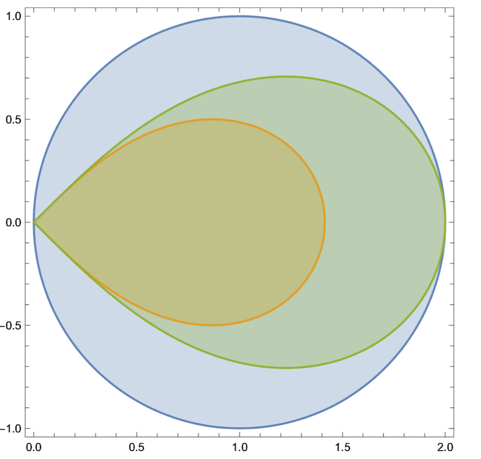
Figure 1: Comparing univalence conditions for $f(z)=z^{c}$

If $-1$ is an eigenvalue of $\hat{B}$ then it is still possible to define the triple $(f,g,B)$ however, where there are eigenvalues of $-1$ the map $f$ will be singular. To do this we note that if $\hat{\lambda}$ is an eigenvalue of $\hat{B}$ then $e^{-2t}\hat{\lambda}$ is an eigenvalue of $\hat{B}_{t}$. In particular, for all $p\in S$ there are at most two values $t$ where $-1$ is an eigenvalue of $\hat{B}_{t}$ so $f_{t}$ and $\hat{f}_{t}$ are defined for all but at most two $t$. If $-1$ is an eigenvalue of $\hat{B}_{t_{0}}$ and is not an eigenvalue of $\hat{B}_{t_{1}}$ then we define $\hat{f}_{t_{0}}(p)={\mathfrak{g}}_{t_{0}-t_{1}}\circ\hat{f}_{t_{1}}(p)$.

If $-1$ is not an eigenvalue of $\hat{B}$ then by Theorem 5.1, the dual pair $(g,B)$ satisfies the Gauss-Codazzi equations in ${{\mathbb{H}}^{3}}$. If $S$ is simply connected then by Theorem 5.12, there is an immersion

$$f\colon S\to{{\mathbb{H}}^{3}}$$

with $g=f^{*}g_{{\mathbb{H}}^{3}}$ and shape operator $B$. Note that $-1$ will not be an eigenvalue of $B$ so by Lemma 5.14, the composition $f_{\infty}={\mathfrak{g}}_{\infty}\circ\hat{f}$ is an immersion.

7 The hyperbolic extension of a projective structure

If a projective structure $\Sigma$ is not simply connected the dual immersions will not map to ${{\mathbb{H}}^{3}}$. Instead we replace ${{\mathbb{H}}^{3}}$ with ${\operatorname{ext}}(\Sigma)$, the hyperbolic extension of $\Sigma$.

We first define this when $\Sigma$ is simply connected. In the general case we will take a quotient.

Let the pair $\Sigma=(S,f)$ define a projective structure with $f\colon S\to\widehat{{\mathbb{C}}}$ and immersion. Then $U\subset S$ is a round disk in $\Sigma$ if $f(U)$ is a round disk. For each round disk $U$ let $\bar{H}_{U}=U\times[0,1]$ and $H_{U}=U\times[0,1)$. We then fix a continuous map $F_{U}\colon\bar{U}_{H}\to\to{{\mathbb{H}}^{3}}\cup\widehat{{\mathbb{C}}}$ such that $F_{U}(z,1)=f(z)$ and $F_{U}$ restricted to $H_{U}$ is a homeomorphism to a closed hyperbolic half-space in ${{\mathbb{H}}^{3}}$. If $U_{0}$ and $U_{1}$ are round disks in $\Sigma$ with $U_{0}\cap U_{1}\neq\emptyset$ then we define $(z_{0},t_{0})\sim(z_{1},t_{1})$ if $F_{U_{0}}(z_{0},t_{0})=F_{U_{1}}(z_{1},t_{1})$. This defines an equivalence relation of the disjoint union of $\bar{H}_{U}$ and the projective extension ${\operatorname{ext}}(\Sigma)$ of $\Sigma$ is the quotient of this union by the equivalence relation $\sim$. Similarly we define ${\operatorname{ext}}^{\rm o}(\Sigma)$ as the subspace of ${\operatorname{ext}}(\Sigma)$ given by the equivalence relation on the disjoint union of $H_{U}$. Then ${\operatorname{ext}}(\Sigma)$ is homeomorphic to $S\times[0,1]$ and there is a map $F\colon{\operatorname{ext}}(\Sigma)\to{{\mathbb{H}}^{3}}\cup\widehat{{\mathbb{C}}}$ such that on each $\bar{U}_{H}$ we have $F=F_{U}$. In particular $F(z,1)=f(z)$. Note that $F$ pulls back a hyperbolic metric to ${\operatorname{ext}}^{\rm o}(\Sigma)$ but the boundary is not smooth. Instead $S\times\{0\}$ is a locally convex pleated surface. We also note that while if $(z_{0},1)\sim(z_{1},t_{1})$ then $t_{1}=1$ in general the equivalence relation does not respect the product structure on the $\bar{U}_{H}$. For further details see [KT].

If $\Sigma$ is a projective structure on a surface $S$ that does not come from a pair $(S,f)$ then we can lift $\Sigma$ to a projective structure $\tilde{\Sigma}$ on the universal cover $\tilde{S}$ of $S$. Then $\tilde{\Sigma}$ does come from a pair $(\tilde{S},f)$ and furthermore the deck action on $\tilde{\Sigma}$ will extend to a deck action on ${\operatorname{ext}}(\tilde{\Sigma})$ where the action on the hyperbolic part of ${\operatorname{ext}}(\tilde{\Sigma})$ will be by isometries. Then the quotient of ${\operatorname{ext}}(\tilde{\Sigma})$ by this deck action will be ${\operatorname{ext}}(\Sigma)$.

7.1 Embedding the flow space in ${\operatorname{ext}}(\Sigma)$

We consider conformal metrics $\hat{g}$ on $\Sigma$ such that the dual pair $(g,B)$ locally convex surfaces. We show that then the associated flow space ${\cal F}_{(g,B)}([0,\infty))$ isometrically embeds in ${\operatorname{ext}}^{\rm o}(\Sigma)$. Further using this, we will show that for two such metrics $\hat{g}_{1},\hat{g}_{2}$ with $\hat{g}_{1}\leq\hat{g}_{2}$ then ${\cal F}_{(g_{2},B_{2})}([0,\infty))$ isometrically embeds in ${\cal F}_{(g_{1},B_{1})}([0,\infty))$.

Proposition 7.1

Let $\hat{g}$ be a conformal metric on a projective structure $\Sigma$ on a surface $S$ with projective shape operator $\hat{B}$ and dual pair $(g,B)$. If $g$ is complete and the eigenvalues $\hat{B}$ are between $(-1,1]$ the flow space ${\cal F}_{(g,B)}([0,\infty))$ isometrically embeds in ${\operatorname{ext}}^{\rm o}(\Sigma)$.

The intersection of $\Sigma\times\{0\}$ with the internal boundary of ${\operatorname{ext}}(\Sigma)$ is a union of plaques.

Proof: First assume that $\Sigma$ is simply connected. By Lemma 5.8 since $g$ is complete the flow space ${\cal F}_{(g,B)}([0,\infty))$ is complete and any piece of a hyperbolic plane tangent to $\Sigma\times\{0\}$ will extend to an immersed copy of ${\mathbb{H}}^{2}$. The local isometry from the flow space to ${{\mathbb{H}}^{3}}$ this plane will be embedded and hence it must be embedded in the flow space. In particular it will extend to a round disk $U$ in $\Sigma$. One can then construct the flow space similarly to the construction of ${\operatorname{ext}}(\Sigma)$ however rather than take all round disks in $\Sigma$ we just take those that arise from tangent planes to $\Sigma\times\{0\}$. Then the resulting quotient space will be a subspace of ${\operatorname{ext}}(\Sigma)$. On the other hand this quotient space will be isometric to the original flow space ${\cal F}_{(g,B)}([0,\infty))$ so the flow space isometrically embeds in ${\operatorname{ext}}^{\rm o}(\Sigma)$.

Note that the construction of ${\operatorname{ext}}(\Sigma)$ and the flow space is canonical so any deck action that preserves both the projective structure and the metric $\hat{g}$ will extends to isometries of ${\operatorname{ext}}(\Sigma)$ and the flow space. In particular the quotient of the flow space (which will be the flow space of the quotient) will isometrically embed in the quotient of ${\operatorname{ext}}(\Sigma)$ (which will be the extension of the quotient). Therefore to prove the proposition when $\Sigma$ isn’t simply connected we lift to the universal cover, construct the embedding there and then take the quotient. $\Box$

There is a natural metric on $\Sigma$ closely associated to ${\operatorname{ext}}(\Sigma)$. As before assume that $\Sigma$ is simply connected. If $U$ is a round disk let $\hat{g}_{U}$ be the hyperbolic metric. Then Thurston defines the projective metric $\hat{g}_{\Sigma}$ to be the infimum, at each point $z\in\Sigma$ of $\hat{g}_{U}$ at $z$ where $U$ varies over all round disks that contain $z$. If $\Sigma$ is hyperbolic then the infimum is realized and $\hat{g}_{\Sigma}$ is everywhere positive. We note that while this metric will be continuous, it will not be smooth. If $\Sigma$ is not simply connected we observe that the projective metric on the universal cover will be equivariant and descend to a metric on $\Sigma$. This is the projective metric $\hat{g}_{\Sigma}$ on $\Sigma$.

An important special cases is when $\Sigma$ is an open domain in $\widehat{{\mathbb{C}}}$. That is $\Omega=\widehat{{\mathbb{C}}}\smallsetminus\Lambda$ for some closed set $\Lambda$ in $\widehat{{\mathbb{C}}}$. The convex hull of $\Lambda$ in ${{\mathbb{H}}^{3}}$ is the smallest, closed convex set whose closure in $\widehat{{\mathbb{C}}}=\partial{{\mathbb{H}}^{3}}$ is $\Lambda$. The convex hull is the intersection of all half spaces in ${{\mathbb{H}}^{3}}$ whose closure in $\widehat{{\mathbb{C}}}$ contains $\Lambda$. Then by definition ${\operatorname{ext}}(\Sigma)$ is the union of the complementary half-spaces. It follows that ${\operatorname{ext}}(\Sigma)$ is the complement of the interior of the convex hull.

Let $\Sigma$ be a projective structure on a simply connected surface $S$ determined by an immersion $f_{\infty}\colon S\to\widehat{{\mathbb{C}}}$. We can assume that the restriction of $F\colon{\operatorname{ext}}(\Sigma)\to{{\mathbb{H}}^{3}}\cup\widehat{{\mathbb{C}}}$ to $\Sigma$ is $f_{\infty}$. If ${\mathfrak{h}}$ is a horoball in ${\operatorname{ext}}(\Sigma)$ based at $z\in\Sigma$ then $F({\mathfrak{h}})$ is a horoball in ${{\mathbb{H}}^{3}}$ based at $w=f_{\infty}(z)$. Then $F({\mathfrak{h}})={\mathfrak{h}}_{g_{w}}(w)$ where $g_{w}$ is a conformal metric for the tangent space $T_{w}\widehat{{\mathbb{C}}}$. If $\hat{g}$ is conformal metric on $\Sigma$ and $\hat{g}=(f_{\infty})^{*}g_{w}$ at $z$ then we write ${\mathfrak{h}}_{\hat{g}}(z)={\mathfrak{h}}$.

The next lemma gives a condition on the conformal metric $\hat{g}$ for the horoballs ${\mathfrak{h}}_{\hat{g}}(z)$ to embed in ${\operatorname{ext}}(\Sigma)$.

Lemma 7.2

If $\hat{g}$ is a conformal metric on a simply connected projective structure $\Sigma$ with $\hat{g}\geq g_{\Sigma}$ then the horoball ${\mathfrak{h}}_{\hat{g}}(z)$ is contained in ${\operatorname{ext}}(\Sigma)$ for all $z\in\Sigma$.

Proof: By the definition of the projective metric for any $z\in\Sigma$ there is a round disk $U$ in $\Sigma$ such that $g_{U}\leq\hat{g}$ at $z$. Then the half space $H_{U}$ will isometrically embed in ${\operatorname{ext}}(\Sigma)$ and the horoball ${\mathfrak{h}}_{g_{U}}(z)$ will be contained in $H_{U}$ and therefore will be contained in ${\operatorname{ext}}(\Sigma)$. As $g_{U}\leq\hat{g}$ at $z$ we also have that ${\mathfrak{h}}_{\hat{g}}(z)$ is contained in ${\mathfrak{h}}_{g_{U}}(z)$ so ${\mathfrak{h}}_{\hat{g}}(z)$ is contained in ${\operatorname{ext}}(\Sigma)$. $\Box$

Proposition 7.3

Let $\hat{g}_{1}$ and $\hat{g}_{2}$ be conformal metrics on a simply connected projective structure and assume that both projective shape operators $\hat{B}_{1},\hat{B}_{2}$ have eigenvalues in the interval $(-1,1]$. If $\hat{g}_{1}\leq\hat{g}_{2}$ then the flow space ${\cal F}_{(g_{2},B_{2})}([0,\infty))$ isometrically embeds in the flow space ${\cal F}_{(g_{1},B_{1})}([0,\infty))$.

Proof: By Proposition 7.1 the flow spaces ${\cal F}_{(g_{i},B_{i})}([0,\infty))$ embed in ${\operatorname{ext}}(\Sigma)$ and is the union of horoballs ${\mathfrak{h}}_{\hat{g}_{i}}(z)$. Since for each $z\in\Sigma$ the horoballs ${\mathfrak{h}}_{\hat{g}_{2}}(z)$ are contained in the horoballs ${\mathfrak{h}}_{\hat{g}_{1}}(z)$ this implies that the flow space ${\cal F}_{(g_{2},B_{2})}([0,\infty))$ isometrically embeds in the flow space ${\cal F}_{(g_{1},B_{1})}([0,\infty))$. $\Box$

7.2 Convexity

We derive a convexity criterion for the dual surface of a pair $(\hat{g},\hat{B})$.

Theorem 7.4

Let $(\Sigma,\hat{g},\hat{B})$ be a projective structure, conformal metric and shape operator with dual triple $(f,g,B)$. Let $f_{t}=\pi\circ{\mathfrak{g}}_{t}\circ\hat{f}$. Then for

$$e^{2t_{0}}>\sup\{|K(\hat{g})|+4\|Q(\Sigma,\hat{g})\|\}$$

$f_{t_{0}}$ is a locally convex immersion. In particular if $g_{\Sigma}$ is the projective metric on $\Sigma$ and $\hat{g}$ is complete then

$$g_{\Sigma}\leq\sup\{|K(\hat{g})|+4\|Q(\Sigma,\hat{g})\|\}\hat{g}.$$

Proof: The map $f_{t}$ has shape operator $B_{t}=({\operatorname{Id}}+e^{-2t}\hat{B})^{-1}({\operatorname{Id}}-e^{-2t}\hat{B})$. Therefore if $\lambda_{0},\lambda_{1}$ are the eigenvalues of $\hat{B}$ the surface given by $f_{t}$ has principal curvatures

$$\frac{1-e^{-2t}\lambda_{i}}{1+e^{-2t}\lambda_{i}}.$$

If $e^{2t_{0}}>\max\{|\lambda_{0}|,|\lambda_{1}|\}$ these are both positive. Therefore if this holds at every point then $f_{t_{0}}$ is an immersion and locally convex. Therefore by the prior lemma

$$\max\{|\lambda_{0}|,|\lambda_{1}|\}=|K(\hat{g})|+4\|Q(\Sigma,\hat{g})\|.$$

Therefore $f_{t}$ is locally convex for $t>\sup\{|K(\hat{g})|+4\|Q(\Sigma,\hat{g})\|\}$. By [BBB], if a complete conformal metric $\hat{g}$ on $\Sigma$ has locally convex immersed surface, then $g_{\Sigma}\leq\hat{g}$ where $g_{\Sigma}$ is the projective metric on $\Sigma$. Therefore for $t>\sup\{|K(\hat{g})|+4\|Q(\Sigma,\hat{g})\|\}$ we have $g_{\Sigma}\leq e^{2t}\hat{g}.$ Taking the infimum over all such $t$ we get

$$g_{\Sigma}\leq\sup\{|K(\hat{g})|+4\|Q(\Sigma,\hat{g})\|\}\hat{g}$$

$\Box$

In [BBB, Theorem 2.8] we prove that for $g_{h}$ the hyperbolic metric then

$$g_{\Sigma}\leq(1+2\|\phi_{\Sigma}\|_{\infty})g_{h}.$$

As $Q(\Sigma,g_{h})=-\phi_{\Sigma}/2$ we see that the above theorem is a generalization for arbitrary conformal metrics.

8 Hyperbolic 3-manifolds

Let $M$ be a hyperbolic 3-manifold. Then $M={{\mathbb{H}}^{3}}/\Gamma$ where the deck group $\Gamma$ is a discrete group of isometries of ${{\mathbb{H}}^{3}}$. The group $\Gamma$ will also act on $\partial{{\mathbb{H}}^{3}}=\widehat{{\mathbb{C}}}$ with domain of discontinuity $\Omega$. Then the quotient $\bar{M}=({{\mathbb{H}}^{3}}\cup\Omega)/\Gamma$ is a 3-manifold with boundary. If $\bar{M}$ is compact then $M$ is a conformally compact hyperbolic 3-manifold. The boundary $\Sigma=\Omega/\Gamma$ is a projective structure and is the projective boundary of $M$. While conformally compact is the usual terminology for Einstein manifolds, for hyperbolic 3-manifolds one usually refers to $\bar{M}$ as convex co-compact because, as we will see shortly, there are convex $\Gamma$-invariant subsets of ${{\mathbb{H}}^{3}}$ with compact $\Gamma$-quotient. We will define a correspondence between convex, compact submanifolds of $M$ and conformal metrics on $\Sigma$ whose projective shape operator has eigenvalues in the interval $(-1,1]$.

We begin with the classical classification of Kleinian groups by their conformal boundary. We’ll state this theorem in a somewhat unusual way that will be convenient for our purposes.

Theorem 8.1

Let $\bar{X}$ be a smooth, compact, 3-manifold with boundary with $X$ the interior of $\bar{X}$. Assume that $\bar{X}$ is homeomorphic to a convex co-compact hyperbolic 3-manifold and let $\hat{g}$ be a smooth Riemannian metric on $\partial\bar{X}$. Then there exists a convex, co-compact hyperbolic 3-manifold $\bar{M}_{\hat{g}}$ and a diffeomorphism $\phi_{\hat{g}}\colon\bar{X}\to\bar{M}_{\hat{g}}$ such that the restriction of $\phi$ to $\partial\bar{X}$ is a conformal map from the conformal class of $\hat{g}$ to $\partial_{c}M$.

Furthermore if $\hat{g}_{0}$ is another Riemannian metric on $\partial\bar{X}$ and there is a diffeomorphism of $\bar{X}$ to itself such the restriction to $\partial\bar{X}$ is a conformal map from the conformal class of $\hat{g}$ to the conformal class of $\hat{g}_{0}$ then there is an isometry from $\bar{M}_{\hat{g}}$ to $\bar{M}_{\hat{g}_{0}}$ whose restriction to the boundary is the given conformal map.

Let ${\mathcal{G}}(\partial\bar{X})$ be the space of smooth Riemannian metrics on $\partial\bar{X}$. Then for $\hat{g}\in{\mathcal{G}}(\partial\bar{X})$ we can use the diffeomorphism $\phi_{\hat{g}}\colon\bar{X}\to\bar{M}_{\hat{g}}$ to pull back the projective structure on $\partial\bar{M}_{\hat{g}}$ to a projective structure $\Sigma_{\hat{g}}$ on $\partial\bar{X}$. Let ${\hat{B}}_{\hat{g}}$ be the projective shape operator and ${\mathcal{G}}_{c}(\partial\bar{X})\subset{\mathcal{G}}(\partial\bar{X})$ the subspace of metrics where ${\hat{B}}_{\hat{g}}$ has eigenvalues in the interval $(-1,1]$.

The pair $(\hat{g},{\hat{B}}_{\hat{g}})$ has a dual pair $(g,B_{g})$. The dual pair determines an isometric immersion $f_{\hat{g}}\colon\partial\bar{X}\to M_{\hat{g}}$. To construct $f_{\hat{g}}$ we observe that the metric $g$ and shape operator lift to the universal cover of each component of $\partial\bar{X}$. We can then construct the isometric immersion on the universal cover and observe that it will descend to the map $f_{\hat{g}}$ by the naturality of the constructions. In fact the same argument gives a local isometry $F\colon{\cal F}_{(g,B_{g})}([0,\infty])\to M_{\hat{g}}$.

The hyperbolic manifold $M={{\mathbb{H}}^{3}}/\Gamma$ is Fuchsian if there is a $\Gamma$-invariant copy of ${\mathbb{H}}^{2}$ in ${{\mathbb{H}}^{3}}$. This equivalent to the limit set of $\Gamma$ being contained in a round circle. The quotient ${\mathbb{H}}^{2}/\Gamma$ is the unique totally geodesic surface in $M$ whose inclusion in $M$ is a homotopy equivalence.

A convex co-compact hyperbolic 3-manifold is Fuchsian if its limit set is a round circle.

Lemma 8.2

Given $\hat{g}\in{\mathcal{G}}_{c}(\partial\bar{X})$ the dual immersion

$$f_{\hat{g}}\colon\partial\bar{X}\to M_{\hat{g}}$$

is an embedding and the image bounds a convex manifold homeomorphic to $\bar{X}$ or $M_{\hat{g}}$ is Fuchsian and $f_{\hat{g}}$ is 2-to-1 with image a totally geodesic surface. In this last case ${\hat{B}}_{\hat{g}}$ is the identity.

Proof: We will show that the map $F\colon{\cal F}\to\bar{M}_{\hat{g}}$ is an embedding unless $M_{\hat{g}}$ is Fuchsian and $\hat{g}$ is the hyperbolic metric. The restriction of $F$ to $\partial\bar{X}\times\{\infty\}$ is a diffeomorphism to $\partial\bar{M}_{\hat{g}}$ and $F$ is an immersion everywhere. Since $\partial\bar{X}$ is compact this implies that $F$ is an embedding on ${\cal F}_{(g,B_{g})}([T,\infty])$ for large $T$. Let $T_{0}$ be the infimum of $T$ where the map is an embedding. Then there must be $p\neq q$ in $S$ such that $F(p,T_{0})=F(q,T_{0})$ and the $F$-image of $S\times\{T_{0}\}$ will be tangent at this point of intersection. Furthermore their normals will be pointing in opposite directions. Convexity then implies that the surfaces are totally geodesic and 2-to-1 on a neighborhood of $p$ and $q$. This open condition is also a closed condition so $F$ will be totally geodesic and 2-to-1 on the components of $\partial\bar{X}\times\{T_{0}\}$ that contain $(p,T_{0})$ and $(q,T_{0})$. Since the surfaces $\partial\bar{X}\times\{t\}$ are strictly convex when $t>0$ this can only happen when $T_{0}=0$. $\Box$

We can also start with a smooth, convex submanifold $N$ of a convex co-compact hyperbolic 3-manifold $M$ and produce a conformal metric $\hat{g}$ on $\partial_{c}M$ such that $N=N_{\hat{g}}$.

Lemma 8.3

Let $N\subset M$ be a convex, compact submanifold of a convex co-compact hyperbolic manifold $M$. If $\Sigma$ is the projective boundary of $M$ then there is a unique conformal metric $\hat{g}$ on $\Sigma$ such that $N_{\hat{g}}=N$.

Proof: We’ll assume that $M={{\mathbb{H}}^{3}}$ and $N$ is closed convex subset of ${{\mathbb{H}}^{3}}$ with smooth boundary and we will find a conformal metric on $\Omega=\widehat{{\mathbb{C}}}\smallsetminus\bar{N}$. Then for each $z\in\Omega$ there is a unique horosphere ${\mathfrak{h}}_{z}$ that intersects $N$ in a single point $p$. We then let $\hat{g}$ be the conformal metric on $\Omega$ with $\hat{g}=\nu_{p}$ at $z$. Then $\partial N$ is the Epstein surface for $\hat{g}$. By Theorem 2.4 we have that $\partial N$ is (the image of) the dual immersion for the pair $(\Omega,\hat{g})$.

When $N$ is a smooth, convex submanifold of a convex co-compact manifold take the pre-image of $N$ in the universal cover ${{\mathbb{H}}^{3}}$ and apply the construction from the previous paragraph to get an equivariant conformal metric on the domain of discontinuity. This will descend to a metric $\hat{g}$ on $\partial\bar{M}$ with $N=N_{\hat{g}}$. $\Box$

We note that the construction of the metric $\hat{g}$ works even when $N$ is convex but not smooth. However, in this case $\hat{g}$ will not be smooth so we cannot construct the dual metric $g$ as in the smooth case. This will be discussed further below.

9 $W$-volume

As in the previous section we fix compact, hyperbolizable 3-manifold $\bar{X}$. We first define the $W$-volume on ${\cal G}_{c}(\partial\bar{X})$. We will then extend it to ${\cal G}(\partial\bar{X})$. Recall that associated to $\hat{g}\in{\cal G}_{c}(\partial\bar{X})$ we have a convex, hyperbolic 3-manifold $N_{\hat{g}}$ that is homeomorphic $\bar{X}$

• $M_{\hat{g}}$ is a convex co-compact hyperbolic structure on $X$ with $\hat{g}$ a conformal metric on $\partial_{c}M_{\hat{g}}$;

• ${\hat{B}}_{\hat{g}}$ is the projective shape operator for the metric $\hat{g}$ and the projective boundary of $M_{\hat{g}}$;

• $(g,B_{g})$ is the pair dual to $(\hat{g},{\hat{B}}_{\hat{g}})$;

• $N_{\hat{g}}$ is a smooth convex submanifold of $M_{\hat{g}}$;

• the induced metric on $\partial N_{\hat{g}}$ is $g$ and the shape operator is $B_{g}$.

The mean curvature $H_{g}$ of $\partial N_{\hat{g}}$ is one half the trace of $B_{g}$ and is a function on $\partial N_{\hat{g}}=\partial\bar{X}$. We define the boundary term

$${\cal B}(\hat{g})=\int_{\partial\bar{X}}H_{g}dA_{g}$$

where $dA_{g}$ is the area form for $g$. Then the $W$-volume is the function $W\colon{\cal G}_{c}(\partial\bar{X})\to\mathbb{R}$ given by

$$W(\hat{g})=\operatorname{vol}(N_{\hat{g}})-\frac{1}{2}{\cal B}(\hat{g}).$$

The space of metric ${\cal G}_{c}(\partial\bar{X})$ is an open subspace of the space of symmetric 2-tensors on $\partial X$ with the $C^{\infty}$-topology. We are interested in calculating the variation of $W$-volume in this topology. More explicitly if $\hat{g}_{t}$ is a smooth family of metrics in ${\cal G}_{c}(\partial\bar{X})$ then we want to find

$$\left.\frac{d}{dt}\right|_{t=0}W(\hat{g}_{t})$$

The smooth family $\hat{g}_{t}$ determines smooth families $B_{\hat{g}_{t}}$, $g_{t}$, $B_{g_{t}}$, etc. Furthermore if $\delta\hat{g}$ is the time zero derivative of $\hat{g}_{t}$ then $\delta\hat{g}$ determines the time zero derivatives $\delta\hat{B}$, $\delta g$, $\delta B$, etc. for the associated objects.

We begin with the generalized Schäfli formula for the change in volume of $N_{\hat{g}}$ due to Rivin-Schlenker. They give a formula for the variation of the volume of a compact hyperbolic $n$-manifold, or more generally, a compact Einstein manifold. We will only state it in the setting we will use and include a proof due to Souam ([Sou]) for completeness. While we only need the statement for smooth manifolds with boundary we state it for manifolds with corners as this will come up in the proof. For a manifold with corners at each point $x$ in the co-dimension two face $E$ there is exterior dihedral angle $\theta_{E}(x)$.

Theorem 9.1 (Rivin-Schlenker, [RS] and Souam, [Sou])

Let $M$ be a compact hyperbolic 3-manifold with corners and $\delta g$ a variation of the hyperbolic metric. Then

$$\delta V=\frac{1}{2}\sum_{E}\int_{E}\delta\theta_{E}dE+\int_{\partial M}\langle g,\delta B\rangle_{g}+\frac{1}{2}\langle\delta g,B\rangle_{g}$$

Proof: We can decompose $M$ into finitely many manifolds with corners each of which embeds in ${{\mathbb{H}}^{3}}$. If we prove the formula for each piece then the terms on the faces that are paired will cancel. The corners will come in two types: some will come from corners of the original manifold while others will be new. In the latter case, after the corners in the pieces are glued the will become a smooth part of the interior, in which cases the total angle will be $0$, or a smooth part of the boundary, in which case the total angle will be $\pi$. In both cases, this implies the total change in dihedral angle is zero and and they will not contribute to the last term of the formula.

We now assume that $M$ is a manifold with corners that embeds in ${{\mathbb{H}}^{3}}$. It will be useful to think of $M$ as both a fixed smooth manifold with corners and as a subspace of ${{\mathbb{H}}^{3}}$. As $M$ embeds in ${{\mathbb{H}}^{3}}$ there is a smooth vector field $\xi$, defined on a neighborhood of $M$, with flow $\phi_{t}$, $g_{t}=\phi_{t}^{*}g_{{{\mathbb{H}}^{3}}}$ and $\delta g$ is the time zero derivative of $g_{t}$. We also assume that $\xi$ is non-zero on $M$. If it isn’t, by compactness, the norm of $\xi$ is bounded on $\partial M$ so we can add an infinitesimal isometry to $\xi$ that is larger than this bound. Then the sum will be non-zero.

The family of metrics $g_{t}$ on $M$ also determines a family of shape operators $B_{t}$ and second fundamental forms ${\rm II}_{t}$ on $\partial M$. When there is a subscript we view the object as being on the fixed manifold $M$.

Fix $u\in T_{x}M$ and define a parameterized surface $\sigma\colon(-\epsilon,\epsilon)^{2}\to{{\mathbb{H}}^{3}}$ such that:

$$\sigma(0,0)=x\qquad\quad\sigma(s,t)=\phi_{t}(\sigma(s,0))\qquad\quad\sigma_{*}(0,0)\frac{\partial}{\partial s}=u.$$

This surface will be singular if $u$ and $\xi$ are parallel. We define the vector field $n$ along $\sigma$ such that $n(s,t)$ is the normal vector to $\phi_{t}(\partial M)$ at $\sigma(s,t)$. If we fix $t$ the covariant derivative of $n$ along the path $s\mapsto\sigma(s,t)$ defines another vector field along $\sigma$ which we label $\hat{B}u$ as we have

$$\hat{B}u(0,t)=(\phi_{t})_{*}(B_{t}u).$$

We can also evaluate the curvature tensor in terms of covariant derivatives along $\sigma$:

$$R(\xi,u)n = \frac{D}{dt}\left(\frac{Dn}{ds}\right)-\frac{D}{ds}\left(\frac{Dn}{dt}\right)$$

$$= \nabla_{\xi}\hat{B}u-\nabla_{u}\left(\nabla_{\xi}n\right).$$

Note that while the parameterized surface may be singular, the vector field $\hat{B}u$ is a well defined vector field along the integral curve of $\xi$ through $x$ and $\nabla_{\xi}$ is a smooth vector field on $\partial M$.

We let ${\langle},{\rangle}$ be the usual inner product on ${{\mathbb{H}}^{3}}$. Since we are in constant curvature $=-1$ we have

$$R(\xi,u)n={\langle}n,\xi{\rangle}u-{\langle}n,u{\rangle}\xi={\langle}n,\xi{\rangle}u.$$

Combining this equation with the one above gives

$$\nabla_{\xi}\hat{B}u={\langle}n,\xi{\rangle}u+\nabla_{u}\nabla_{\xi}n.$$

Given any vector $v\in T_{x}M$ we define $\tilde{v}$ to be the parallel vector field on $(-\epsilon,\epsilon)^{2}$ such that $\sigma_{*}(0,0)\tilde{v}=v$. On the integral curve of $\xi$ through $x$ this determines a vector field which we also label $\tilde{v}$. We then have

$$g_{t}(u,v)={\langle}\tilde{u}(\phi_{t}(x)),\tilde{v}(\phi_{t}(x)){\rangle}$$

and

$$\delta g(u,v)=\xi{\langle}\tilde{u},\tilde{v}{\rangle}={\langle}\nabla_{\xi}\tilde{u},v{\rangle}+{\langle}u,\nabla_{\xi}\tilde{v}{\rangle}.$$

As ${\rm II}_{t}(u,v)={\langle}\hat{B}u,\tilde{v}{\rangle}$ at $\phi_{t}(x)$ then

$$\delta{\rm II}(u,v)={\langle}\nabla_{\xi}\hat{B}u,v{\rangle}+{\langle}Bu,\nabla_{\xi}\tilde{v}{\rangle}.$$

On the other hand

$$\delta{\rm II}(u,v)=\delta(g(Bu,v))=\delta g(Bu,v)+{\langle}\delta Bu,v{\rangle}.$$

Combining we get

$${\langle}\delta Bu,v{\rangle} = \delta{\rm II}(u,v)-\delta g(Bu,v)$$

$$= {\langle}\nabla_{\xi}\hat{B}u,v{\rangle}+{\langle}Bu,\nabla_{\xi}\tilde{v}{\rangle}-{\langle}\nabla_{\xi}\widetilde{Bu},v{\rangle}-{\langle}Bu,\nabla_{\xi}\tilde{v}{\rangle}$$

$$= {\langle}\nabla_{\xi}\hat{B}u,v{\rangle}-{\langle}\nabla_{\xi}\widetilde{Bu},v{\rangle}.$$

Substituting for $\nabla_{\xi}\hat{B}u$ we get

$${\langle}n,\xi{\rangle}{\langle}u,v{\rangle}=-{\langle}\nabla_{\tilde{u}}\nabla_{\xi}n,v{\rangle}+{\langle}\nabla_{\xi}\widetilde{Bu},v{\rangle}+{\langle}\delta Bu,v{\rangle}.$$

This expression gives a relationship between four bilinear maps in $u$ and $v$. We will take the trace of each of them. For the term on the left the trace is $2{\langle}n,\xi{\rangle}$. The trace of ${\langle}\nabla_{u}\left(\nabla_{\xi}n\right),v{\rangle}$ is the divergence of $\nabla_{\xi}n$ with respect to the induced metric on $\partial M$. For the middle term on the right we assume that $u$ is an eigenvector of $B$ with eigenvalue of $\lambda$ and noting that $\widetilde{Bu}=\lambda\tilde{u}$ we get

$$\delta g(Bu,u)={\langle}\nabla_{\xi}\widetilde{Bu},u{\rangle}+{\langle}Bu,\nabla_{\xi}\tilde{u}{\rangle}=2\lambda{\langle}\nabla_{\xi}\tilde{u},u{\rangle}=2{\langle}\nabla_{\xi}\widetilde{Bu},u{\rangle}$$

and therefore the trace of $\frac{1}{2}\delta g(Bu,v)$ is equal to the trace of ${\langle}\nabla_{\xi}\widetilde{Bu},v{\rangle}$. In our notation from section 3.1 this gives

$${\langle}\xi,n{\rangle}dA=-\frac{1}{2}\operatorname{div}_{\partial M}\left(\nabla_{\xi}n\right)dA+{\langle}g,\delta B{\rangle}_{g}+\frac{1}{2}{\langle}\delta g,B{\rangle}_{g}$$

By the divergence theorem we have

$$\delta V=\int_{\partial M}\langle\xi,n\rangle dA$$

where $n$ is the outward normal on $\partial M$ and $dA$ is the area form. We note that the divergence theorem holds for manifolds with corners. Thus

$$\delta V=\int_{\partial M}\left(-\frac{1}{2}\operatorname{div}_{\partial M}\left(\nabla_{\xi}n\right)dA+{\langle}g,\delta B{\rangle}_{g}+\frac{1}{2}{\langle}\delta g,B{\rangle}_{g}\right).$$

Finally we consider the divergence term $\operatorname{div}_{\partial M}\left(\nabla_{\xi}n\right)dA$. We note that as $\langle n,n\rangle=1$ then differentiating we have $\langle\nabla_{\xi}n,n\rangle=0.$ Thus $\nabla_{\xi}n$ is a tangent vector on $\partial M$ and smooth except on the edges $E$. Each edge $E$ belongs to exactly two faces $F^{\pm}_{E}$ whose normal $n^{\pm}_{E}$ extends to $E$. Further we define the conormal $v_{E}^{\pm}$ to $E$ to be the normal to $E$ in the face $F^{\pm}_{E}$. Then the divergence theorem, applied to each face, gives

$$\int_{\partial M}\operatorname{div}_{\partial M}(\nabla_{\xi}n)dA=\sum_{E}\int_{E}\langle\nabla_{\xi}n^{+}_{E},v^{+}_{E}\rangle+\langle\nabla_{\xi}n^{-}_{E},v^{-}_{E}\rangle{d\ell}.$$

As $\langle n^{+}_{E},n^{-}_{E}\rangle=\cos\theta_{E}$, differentiating, we get

$$\langle\nabla_{\xi}n^{+}_{E},n^{-}_{E}\rangle+\langle n^{+}_{E},\nabla_{\xi}n^{-}_{E}\rangle=-\sin\theta_{E}\delta\theta_{E}.$$

Also as $n^{+}_{E}$ and $v^{+}_{E}$ are an orthonormal basis for the 2-plane orthogonal to $E$ and $\langle\nabla_{\xi}n^{+}_{E},n^{+}_{E}\rangle=0$ we have

$$\nabla_{\xi}n^{+}_{E}-{\langle}\nabla_{\xi}n^{+}_{E},v^{+}_{E}{\rangle}v^{+}_{E}$$

is tangent to $E$. Therefore the inner produce with $n^{-}_{E}$ is zero giving

$$\langle\nabla_{\xi}n^{+}_{E},n^{-}_{E}\rangle=\langle\nabla_{\xi}n^{+}_{E},v^{+}_{E}\rangle\langle v^{+}_{E},n^{-}_{E}\rangle.$$

As $\langle v^{+}_{E},n^{-}_{E}\rangle=\sin(\theta_{E})$ (and similarly $\langle v^{-}_{E},n^{+}_{E}\rangle=\sin(\theta_{E})$) we have

$$-\sin(\theta_{E})\delta\theta_{E}=(\langle\nabla_{\xi}n^{+}_{E},v^{+}_{E}\rangle+\langle\nabla_{\xi}n^{-}_{E},v^{-}_{E}\rangle)\sin(\theta_{E}).$$

Canceling, we obtain the equation

$$\langle\nabla_{\xi}n^{+}_{E},v^{+}_{E}\rangle+\langle\nabla_{\xi}n^{-}_{E},v^{-}_{E}\rangle=-\delta\theta_{E}.$$

The result follows. $\Box$

Next we state Krasnov and Schlenker’s variation formula for $W$-volume in terms of the interior data.

Theorem 9.2 (Krasnov-Schlenker, [KS1])

Let $M$ be a compact hyperbolic 3-manifold with boundary and $\delta g$ a variation of the hyperbolic metric. If $\delta W$ is the induced variation of the $W$-volume then

$$\delta W=\frac{1}{2}\int_{\partial M}\langle g,\delta B\rangle_{g}+\langle\delta g,B_{0}\rangle_{g}$$

where $(g,B)$ is the dual pair, $B_{0}$ is the traceless part of $B$ and $\delta g$ and $\delta B$ are the induced variations.

Proof: Let $\eta$ be the tangent bundle isomorphism such that $\delta g=2g\cdot\eta$. Then

$$\delta(dA_{g})=\operatorname{Tr}(\eta)dA_{g}=\frac{1}{2}\operatorname{Tr}_{g}(\delta g)dA_{g}=\langle\delta g,{\operatorname{Id}}\rangle_{g}.$$

Applying the formula for $\delta V$ from Theorem 9.1 we have

$$\delta W = \delta V-\delta{\cal B}$$

$$= \int\langle g,\delta B\rangle_{g}+\frac{1}{2}\langle\delta g,B\rangle_{g}-\frac{1}{2}\int\delta HdA_{g}+H\delta(dA_{g})$$

$$= \int\langle g,\delta B\rangle_{g}+\frac{1}{2}\langle\delta g,B\rangle_{g}-\frac{1}{2}\int\langle g,\delta B\rangle_{g}+H\langle\delta g,{\operatorname{Id}}\rangle_{g}$$

$$= \frac{1}{2}\int\langle g,\delta B\rangle_{g}+\langle\delta g,B-H{\operatorname{Id}}\rangle_{g}$$

$$= \frac{1}{2}\int\langle g,\delta B\rangle_{g}+\langle\delta g,B_{0}\rangle_{g}.$$

$\Box$

Krasnov-Schlenker also gave a variational formula for $W$-volume in terms of data at infinity. We show that this formula follows directly from Lemma 3.5 comparing the variation of a pair of metrics.

Theorem 9.3 (Krasnov-Schlenker, [KS1])

Given $\hat{g}\in{\cal G}_{c}(\partial\bar{X})$ and $\delta\hat{g}$ a variation of $\hat{g}$. If $\delta W$ is the induced variation of the $W$-volume then

$$\delta W=-\frac{1}{4}\int_{\partial\bar{X}}\langle\hat{g},\delta\hat{B}\rangle_{\hat{g}}+\langle\delta\hat{g},\hat{B}_{0}\rangle_{\hat{g}}.$$

where $\hat{B}_{0}$ is the traceless part of the shape operator at infinity $\hat{B}$.

Proof: We have $\hat{g}=P^{*}g$ and $g=\hat{P}^{*}\hat{g}$ where

$$P={\operatorname{Id}}+B\qquad\mbox{and}\qquad\hat{P}=\frac{1}{2}({\operatorname{Id}}+\hat{B}).$$

Further as $\hat{g}\in{\cal G}_{c}(\partial\bar{X})$ then $\det({\operatorname{Id}}+B)>0$. Then by Lemma 3.5

$$\langle g,\delta P\rangle_{g}+\langle\delta g,P_{0}\rangle_{g}=-\langle\hat{g},\delta\hat{P}\rangle_{\hat{g}}-\langle\delta\hat{g},\hat{P}_{0}\rangle_{\hat{g}}.$$

As

$$P_{0}=B_{0}\qquad\delta P=\delta B,\qquad\mbox{and}\qquad P_{0}=\frac{1}{2}\hat{B}_{0}\qquad\delta\hat{P}=\frac{1}{2}\delta\hat{B},$$

then by linearity

$$\langle g,\delta B\rangle_{g}+\langle\delta g,B_{0}\rangle_{g}=-\frac{1}{2}\left(\langle\hat{g},\delta\hat{B}\rangle_{\hat{g}}+\langle\delta\hat{g},\hat{B}_{0}\rangle_{\hat{g}}\right).$$

$\Box$

We finally give the variational formula in terms of the Osgood-Stowe differential.

Theorem 9.4

The variational formula for $W$-volume on $\mathcal{G}_{c}(\partial\bar{X})$ at a metric $\hat{g}$ is given by

$$\delta W=\frac{1}{4}\int_{\partial\bar{X}}\delta KdA_{\hat{g}}-2\operatorname{Re}\int_{\partial\bar{X}}\langle Q(\hat{g}),\mu(\delta\hat{g})\rangle_{\hat{g}}.$$

Proof: By [KS1] (see also Theorem 9.3 above)

$$\delta W=-\frac{1}{4}\int\langle\hat{g},\delta\hat{B}\rangle_{\hat{g}}+\langle\delta\hat{g},\hat{B}_{0}\rangle_{\hat{g}}.$$

By the projective Gauss equation we have $\operatorname{Tr}(\hat{B})=-2K(\hat{g})$ which gives

$$\langle\hat{g},\delta\hat{B}\rangle_{\hat{g}}=\frac{1}{2}\operatorname{Tr}(\delta\hat{B})dA_{\hat{g}}=-\delta K(\hat{g})dA_{\hat{g}}.$$

By Theorem 5.15 we have

$$\hat{{\rm II}}_{0}=2{\operatorname{\bf{OS}}}(\Sigma,\hat{g})=2Q(\Sigma,\hat{g})+2\overline{Q(\Sigma,\hat{g})}.$$

We have $\delta\hat{g}=2\hat{g}\cdot\eta$ where the strain $\eta_{0}$ is

$$\eta_{0}=\nu(\delta\hat{g}){\partial_{z}}\otimes d{\overline{z}}+\overline{\nu(\delta\hat{g})}{\partial_{\overline{z}}}\otimes dz$$

and $\mu(\delta\hat{g})=\nu(\delta\hat{g}){\partial_{z}}\otimes d{\overline{z}}$. Thus as $\hat{{\rm II}}_{0}=\hat{g}\cdot\hat{B}_{0}$ we have by Lemma 3.4

$$\langle\delta\hat{g},\hat{B}_{0}\rangle_{\hat{g}}=\langle 2\hat{g}\cdot\eta,\hat{B}_{0}\rangle_{\hat{g}}=\langle\hat{g}\cdot\hat{B}_{0},2\eta\rangle_{\hat{g}}=\langle\hat{{\rm II}}_{0},2\eta_{0}\rangle_{\hat{g}}=8\operatorname{Re}\langle Q(\Sigma,\hat{g}),\mu(\delta\hat{g})\rangle_{\hat{g}}.$$

Substituting, the variational formula follows. $\Box$

9.1 Conformal variations

If we fix the conformal class of the metric $\hat{g}$ then we are fixing the convex co-compact hyperbolic 3-manifold $M_{\hat{g}}$ so we are studying the $W$-volume of convex submanifolds of $M_{\hat{g}}$. We note that the second term in Theorem 9.4 vanishes. This will allow us to make explicit computations which will enable to us to give a general definition of $W$-volume for any smooth metric on $\partial\bar{X}$.

We now prove Theorem 2.8 but only for metrics in ${\cal G}_{c}(\partial\bar{X})$. Once we have done this we will be able to define $W$-volume for general metrics.

Proposition 9.5

Let $\hat{g}\in{\cal G}_{c}(\partial\bar{X})$ and $u$ a smooth function on $\partial\bar{X}$ such that $\hat{g}_{t}=e^{2tu}\hat{g}$ is in ${\cal G}_{c}(\partial\bar{X})$ for $t\in[0,1]$. Then

$$W(\hat{g}_{1})-W(\hat{g}_{0})=-\frac{1}{4}\int_{\partial\bar{X}}u\left(\Omega_{\hat{g}_{0}}+\Omega_{\hat{g}_{1}}\right).$$

Proof: Let $K_{t}=K(\hat{g}_{t})$ be the Gaussian curvature of $\hat{g}_{t}$ and $dA_{t}$ be the area forms. For this proof we need more than the time zero derivative so we let $\dot{K}_{t}$, $\dot{dA}_{t}$, etc. represent time $t$ derivatives. By Gauss-Bonnet

$$\int K_{t}dA_{t}=2\pi\chi(\partial M)$$

so

$$\int\dot{K}_{t}dA_{t}=-\int K_{t}\dot{dA}_{t}.$$

As $dA_{t}=e^{2tu}dA$ we also have $\dot{dA_{t}}\ =2udA_{t}$. As the family $\hat{g}_{t}$ fixes the conformal structure there is only the curvature term in the formula from Theorem 9.4 and we have

$$\dot{W}_{t}=-\frac{1}{4}\int K_{t}\dot{dA}_{t}=-\frac{1}{2}\int uK_{t}dA_{t}.$$

The formula for curvature under conformal change (see [Bes, Theorem 1.159]) gives

$$K_{t}=e^{-2tu}(K(\hat{g})-t\Delta u),$$

where $\Delta$ is the Laplacian of $\hat{g}$. Therefore

$$\dot{W}_{t}=-\frac{1}{2}\int u(K(\hat{g})-t\Delta u)dA_{\hat{g}}=-\frac{1}{2}\int uK(\hat{g})dA_{\hat{g}}+\frac{1}{2}t\int u\Delta udA_{\hat{g}}$$

Integrating we have

$$W(\hat{g}_{1})=W(\hat{g})-\frac{1}{2}\int u\cdot K(\hat{g})dA_{g}+\frac{1}{4}\int u\Delta(u)dA_{g}.$$

Then $K(h)=e^{-2u}(K(g)-\Delta u)$ giving

$$W(h)=W(g)-\frac{1}{4}\int u\cdot K(g)dA_{g}-\frac{1}{4}\int uK(h)dA_{h}$$

Therefore

$$W(h)-W(g)=-\frac{1}{4}(\Omega_{g}+\Omega_{h})(u).$$

$\Box$

We then get Krasnov-Schlenker’s scaling formula for metrics in ${\cal G}_{c}(\partial\bar{X})$.

Corollary 9.6 (Krasnov-Schlenker, [KS1])

If $g\in{\cal G}_{c}(\partial\bar{X})$ and $s\geq 0$ then

$$W\left(e^{2s}\hat{g}\right)=W(\hat{g})-s\pi\chi(\partial\bar{X}).$$

Proof: When $s\geq 0$ the metrics $e^{2t\cdot s}\hat{g}$ are in ${\cal G}_{c}(\partial\bar{X})$ for $t\in[0,1]$ so we can apply Proposition 9.5 with $u\equiv s$. The result then follows by observing that

$$\int_{\partial\bar{X}}s\left(\Omega_{\hat{g}_{0}}+\Omega_{\hat{g}_{1}}\right)=2s(2\pi\chi(\partial\bar{X}))$$

by Gauss-Bonnet. $\Box$

We can now define $W$-volume for an arbitrary $\hat{g}\in{\cal G}(\partial\bar{X})$ as follows. By compactness the absolute value of eigenvalues of $\hat{B}_{\hat{g}}$ are bounded by some constant $\Lambda>1$. Then for and $s>\frac{1}{2}\log\Lambda$ we have that the projective shape operator of the metric $e^{2s}\hat{g}$ has eigenvalues in the interval $(-1,1)$ by Proposition 5.4. We then set

$$W(\hat{g})=W(e^{2s}\hat{g})+s\pi\chi(\partial\bar{X}).$$

and observe that $W(\hat{g})$ doesn’t depend on the choice of $s$ by Corollary 9.6.

We now observe that the results on $W$-volume on ${\cal G}_{c}(\partial\bar{X})$ extend to ${\cal G}(\partial\bar{X})$. As already noted the scaling property is due to Krasnov-Schlenker (see [KS1]).

Theorem 9.7

The following hold for $W$ on ${\cal G}(\partial\bar{X})$.

• If $\hat{g}\in{\cal G}(\partial\bar{X})$ and $s\in\mathbb{R}$ then

  $$W\left(e^{2s}\hat{g}\right)=W(\hat{g})-s\pi\chi(\partial\bar{X}).\qquad\mbox{\bf[Krasnov-Schlenker, \cite[cite]{[\@@bibref{}{KS08}{}{}]}]}$$

• The variational formula for $W$-volume on ${\cal G}(\partial\bar{X})$ at a metric $\hat{g}$ is given by

  $$\delta W=\frac{1}{4}\int_{\partial\bar{X}}\delta KdA_{\hat{g}}-2\operatorname{Re}\int_{\partial\bar{X}}\langle Q(\hat{g}),\mu(\delta\hat{g})\rangle_{\hat{g}}.$$

• Let $\hat{g}_{0},\hat{g}_{1}\in{\cal G}(\partial\bar{X})$ and $u$ a smooth function on $\partial\bar{X}$ such that $\hat{g}_{1}=e^{2u}\hat{g}_{0}$. Then

  $$W(\hat{g}_{1})-W(\hat{g}_{0})=-\frac{1}{4}\int_{\partial\bar{X}}u\left(\Omega_{\hat{g}_{0}}+\Omega_{\hat{g}_{1}}\right).$$

Proof: The first item follows trivially from the definition.

For the variational formula we let $\hat{g}_{t}$ be a variation with $\hat{g}_{0}=\hat{g}$ and $\delta W,\delta K,\delta\hat{g}$ be the derivatives at $t=0$. We fix $s$ such that $e^{2s}\hat{g}_{t}\in{\cal G}_{c}(\partial\bar{X})$ for $t\in(-\epsilon,\epsilon)$. Then by definition

$$W(\hat{g}_{t})=W(e^{2s}\hat{g}_{t})-s\pi\chi(\partial\bar{X}).$$

It follows that

$$\delta W=\frac{1}{4}\int_{\partial\bar{X}}\delta K(e^{2s}\hat{g}_{t})dA_{e^{2s}\hat{g}}-2\operatorname{Re}\int_{\partial\bar{X}}\langle Q(e^{2s}\hat{g}),\mu(\delta(e^{2s}\hat{g}))\rangle_{e^{2s}\hat{g}}.$$

We have $K(e^{2s}\hat{g}_{t})=e^{-2s}K(\hat{g}_{t})$ giving $\delta K(e^{2s}\hat{g}_{t})=e^{-2s}\delta K$. Also $dA_{e^{2s}\hat{g}}=e^{2s}dA_{\hat{g}}$. Further $Q(e^{2s}\hat{g})=Q(\hat{g})$, and $\mu(\delta(e^{2s}\hat{g}))=\mu(\delta\hat{g})$. Finally $\langle\cdot,\cdot\rangle_{\hat{g}}=\langle\cdot,\cdot\rangle_{e^{2s}\hat{g}}$ as the pairing only depends on the conformal class of the metric. Thus

$$\delta W=\frac{1}{4}\int_{\partial\bar{X}}\delta KdA_{\hat{g}}-2\operatorname{Re}\int_{\partial\bar{X}}\langle Q(\hat{g}),\mu(\delta\hat{g})\rangle_{\hat{g}}.$$

For the last item, let $\hat{g}_{t}=e^{2tu}\hat{g}_{0}$. By compactness of $\partial\bar{X}$ we can choose a $T$ such that $e^{2T}\hat{g}_{t}\in{\cal G}_{c}(\partial\bar{X})$ for all $t\in[0,1]$. Also the curvature form in invariant under scaling the metric giving $\Omega_{e^{2T}\hat{g}_{i}}=\Omega_{\hat{g}_{i}}$. Thus

$$W(\hat{g}_{1})-W(\hat{g}_{0})=W(e^{2T}\hat{g}_{1})-W(e^{2T}\hat{g}_{0})=-\frac{1}{4}\int_{\partial\bar{X}}u\left(\Omega_{\hat{g}_{0}}+\Omega_{\hat{g}_{1}}\right).$$

$\Box$

We can now prove our generalization of the Krasnov-Schlenker maximality property.

Theorem 2.9 Let $\hat{g}$ be a constant curvature metric on $\partial\bar{X}$ and let $\hat{h}=e^{2u}\hat{g}$ be a smooth metric on $\partial\bar{X}$ with the same area as $\hat{g}$. Then

$$W(\hat{g})-W\left(\hat{h}\right)\geq\frac{1}{4}\|\nabla u\|_{2}^{2}$$

where $\nabla$ is the gradient of $\hat{g}$.

Proof: Assume $\hat{g}$ has constant curvature $K<0$. If $\Delta$ is the Laplacian of $\hat{g}$, then $K(\hat{h})=e^{-2u}(K-\Delta u)$. Then by Theorem 2.8

$$W(\hat{g})-W\left(\hat{h}\right)=\frac{1}{4}\int u(\Omega_{\hat{g}}+\Omega_{\hat{h}})=-\frac{1}{4}\int u(\Delta u-2K)dA_{\hat{g}}.$$

Then by the divergence theorem applied to $u\nabla u$ we have Green’s identity

$$0=\int\nabla\cdot(u\nabla u)dA_{\hat{g}}=\int u\Delta udA_{\hat{g}}+\int\nabla u\cdot\nabla u\ dA_{\hat{g}}=\int u\Delta udA_{\hat{g}}+\|\nabla u\|_{2}^{2}.$$

Thus as $t\leq e^{t}-1$ for all $t\in\mathbb{R}$ and $K$ is non-positive,

$$W(\hat{g})-W(\hat{h})-\frac{1}{4}\|\nabla u\|_{2}^{2}=\frac{K}{4}\int 2udA_{\hat{g}}\geq\frac{K}{4}\int(e^{2u}-1)dA_{\hat{g}}=\frac{K}{4}\int dA_{\hat{h}}-dA_{\hat{g}}=0$$

as $\hat{g},\hat{h}$ have the same area. $\Box$

9.2 $W$-volume for projective structures

We now define a relative version of $W$-volume and show that it naturally extends to a pair of conformal metrics on an arbitrary projective structure. In earlier work (see [KS2]) Krasnov-Schlenker define this for two conformal metrics on a projective structure where one is the projective metric.

We will see that much of the theory for $W$-volume for convex co-compact $3$-manifolds easily extends to this $W$-volume for pairs. We will also show that we can use this $W$-volume for pairs to obtain a surprising bound on the $L^{2}$-norm of a projective structure in terms of the length of the associated bending measured lamination.

Let $\hat{g}_{0},\hat{g}_{1}\in{\cal G}(\partial\bar{X})$ be in the same conformal class and define

$$W(\hat{g}_{0},\hat{g}_{1})=W(\hat{g}_{1})-W(\hat{g}_{0}).$$

Of course this definition makes sense for any pair of metrics in ${\cal G}(\partial\bar{X})$. However, when the metrics are in the same conformal class $N_{\hat{g}_{0}}$ and $N_{\hat{g}_{1}}$ are both submanifolds of the same convex co-compact hyperbolic 3-manifold. In fact if $N_{\hat{g}_{0}}\subset N_{\hat{g}_{1}}$ then

$$W(\hat{g}_{0},\hat{g}_{1})=\operatorname{vol}(N_{\hat{g}_{1}}\smallsetminus N_{\hat{g}_{0}})-\frac{1}{2}\left({\cal B}(\hat{g}_{1})-{\cal B}(\hat{g}_{0})\right).$$

With this as motivation we now define a relative $W$-volume for pairs of conformal metrics on a projective structure. Let $\Sigma$ be a projective structure and let ${\cal G}(\Sigma)$ be smooth conformal metrics on $\Sigma$ and ${\cal G}_{c}(\Sigma)$ the subspace of metrics such that the projective shape operator has eigenvalues in the interval $(-1,1]$. For $\hat{g}\in{\cal G}_{c}(\Sigma)$ by Proposition 7.1 the flowspace ${\cal F}_{(g,B)}([0,\infty))$ embeds in ${\operatorname{ext}}^{\rm o}(\Sigma)$ with compact complement. We define $N_{\hat{g}}={\operatorname{ext}}^{\rm o}(\Sigma)\backslash{\cal F}_{(g,B)}((0,\infty))$. Then for $\hat{g},\hat{h}\in{\cal G}_{c}(\Sigma)$ we define

$$W(\hat{g},\hat{h})=\operatorname{vol}(N_{\hat{h}})-\operatorname{vol}(N_{\hat{g}})-\frac{1}{2}({\cal B}(\hat{h})-{\cal B}(\hat{g})).$$

We would like to extend this definition to arbitrary pairs of conformal metrics. Our strategy will be the same as when we were considering convex hyperbolic 3-manifolds. In particular, the variational formulas will continue to hold with the only change being that in the definition of $W(\hat{g}_{0},\hat{g}_{1})$ the boundary ${\cal B}(\hat{g}_{0})$ is positive so in the variational formulas the term coming from the variation of $\hat{g}_{0}$ will have opposite sign. It follows that given $\hat{g}_{0},\hat{g}_{1}\in{\cal G}_{c}(\Sigma)$ and $t\geq s\geq 0$ we have

$$W(\hat{g}_{0},\hat{g}_{1})=W(e^{2t}\hat{g}_{0},e^{2s}\hat{g}_{1})-(t-s)\pi\chi(\Sigma).$$

Then for two arbitrary smooth metrics $\hat{g}_{0},\hat{g}_{1}\in{\cal G}(\Sigma)$ we can choose $s$ and $t$ such that $e^{2t}\hat{g}_{0},e^{2s}\hat{g}_{1}\in{\cal G}_{c}(\Sigma)$ and define

$$W(\hat{g}_{0},\hat{g}_{1})=W(e^{2t}\hat{g}_{0},e^{2s}\hat{g}_{1})-(t-s)\pi\chi(\Sigma).$$

As before the choice of $s$ and $t$ aren’t unique but the definition of $W(\hat{g}_{0},\hat{g}_{1})$ is independent of this choice.

The following properties of W-volume for pairs of metrics in ${\cal G}(\Sigma)$ follows easily from Theorem 9.7.

Theorem 9.8

The following hold for $W$ on ${\cal G}(\Sigma)$.

• If $\hat{g}_{0},\hat{g}_{1}\in{\cal G}(\Sigma)$ and $s,t\in\mathbb{R}$ then

  $$W(\hat{g}_{0},\hat{g}_{1})=W(e^{2t}\hat{g}_{0},e^{2s}\hat{g}_{1})-(t-s)\pi\chi(\Sigma).$$

• The variational formula for $W$-volume at $(\hat{g}_{0},\hat{g}_{1})\in{\cal G}(\Sigma)\times{\cal G}(\Sigma)$ is

  $$\delta W=\frac{1}{4}\int_{\Sigma}\delta K(\hat{g}_{1})dA_{\hat{g}_{1}}-\delta K(\hat{g}_{0})dA_{\hat{g}_{0}}$$

• Let $\hat{g}_{0},\hat{g}_{1}\in{\cal G}(\Sigma)$ and $u$ a smooth function such that $\hat{g}_{1}=e^{2u}\hat{g}_{0}$. Then

  $$W(\hat{g}_{0},\hat{g}_{1})=-\frac{1}{4}\int_{\Sigma}u\left(\Omega_{\hat{g}_{0}}+\Omega_{\hat{g}_{1}}\right).$$

  In particular if $\hat{g}_{0},\hat{g}_{1}$ are non-positively curved with $\hat{g}_{1}\leq\hat{g}_{0}$ then

  $$W(\hat{g}_{0},\hat{g}_{1})\leq 0.$$

• If $\hat{g}_{0}$ is constant curvature and $\hat{g}_{1}=e^{2u}\hat{g}_{0}$ has the same area as $\hat{g}_{0}$ then

  $$W(\hat{g}_{0},\hat{g}_{1})\leq-\frac{1}{4}\|\nabla u\|_{2}^{2}$$

  where $\nabla$ is the gradient for $\hat{g}_{0}$.

Proposition 9.9

If $\hat{g}_{0},\hat{g}_{1}\in{\cal G}_{c}(\Sigma)$ with $\hat{g}_{0}\leq\hat{g}_{1}$ then

$$W(\hat{g}_{0},\hat{g}_{1})\geq\frac{1}{2}\left({\cal B}(\hat{g}_{0})-{\cal B}(\hat{g}_{1})\right).$$

Proof: Since $\hat{g}_{0},\hat{g}_{1}\in{\cal G}_{c}(\Sigma)$ and $\hat{g}_{0}\leq\hat{g}_{1}$ then by Proposition 7.3 $N_{\hat{g}_{0}}\subseteq N_{\hat{g}_{1}}$. Therefore

$$W(\hat{g}_{0},\hat{g}_{1}) = \operatorname{vol}\left(N_{\hat{g}_{1}})-\operatorname{vol}(N_{\hat{g}_{0}}\right)-\frac{1}{2}\left({\cal B}\left(\hat{g}_{1}\right)-{\cal B}\left(\hat{g}_{0}\right)\right)$$

$$\geq \frac{1}{2}\left({\cal B}\left(\hat{g}_{0}\right)-{\cal B}\left(\hat{g}_{1}\right)\right)$$

$\Box$

9.3 $W(\hat{g}_{h},\hat{g}_{\Sigma})$

To prove Theorem 2.10, we will obtain upper and lower bounds on $W(\hat{g}_{h},\hat{g}_{\Sigma})$. As the projective metric $\hat{g}_{\Sigma}$ is not smooth, we first need to extend $W$. We define ${\cal G}^{0}_{c}(\Sigma)=\overline{{\cal G}^{0}_{c}(\Sigma)}\subseteq{\cal G}^{0}(\Sigma)$ where the closure is with respect to the sup-norm topology on the space of continuous conformal metrics ${\cal G}^{0}(\Sigma)$. In the appendix we will show that $W$ extends continuously to ${\cal G}^{0}_{c}(\Sigma)\times{\cal G}^{0}_{c}(\Sigma)$ and that $\hat{g}_{\Sigma}\in{\cal G}^{0}_{c}(\Sigma)$. This will suffice for our purposes.

To get an upper bound we will rescale the metrics so that they have the same area and the use the maximality property for metrics of constant curvature. For the lower bound we scale the hyperbolic metric so that its Epstein surface is convex and then we’ll apply Proposition 9.9. For the first estimate we need a formula for the area of the projective metric $\hat{g}_{\Sigma}$. For the second we will need formulas for the areas of the scaled metrics $(\hat{g}_{h})_{t}$ and $(\hat{g}_{\Sigma})_{t}$ and their Epstein surfaces. We begin with hyperbolic metric:

Lemma 9.10

Let $\hat{g}_{h}$ be the hyperbolic metric on $\Sigma$ and $(g_{h})_{t}$ the dual metrics to $e^{2t}\hat{g}_{h}$. Then for $t>\frac{1}{2}\log\left(1+2\left\|\Phi_{\Sigma}\right\|_{\infty}\right)$ we have

$${\operatorname{{\bf area}}}((g_{h})_{t})=-2\pi\chi(\Sigma)\cosh^{2}(t)-e^{-2t}\left\|\Phi_{\Sigma}\right\|^{2}_{2}.$$

Proof: If $d{\hat{A}}_{t}$ is the area form for $(\hat{g}_{h})_{t}$ and $dA_{t}$ is the area form for $g_{t}$ then by Proposition 5.4 we have

$$dA_{t}=\frac{1}{4}\left|\det\left({\operatorname{Id}}+\hat{B}_{t}\right)\right|d\hat{A}_{t}=\frac{1}{4}\left|\det\left({\operatorname{Id}}+e^{-2t}\hat{B}_{0}\right)\right|e^{2t}d\hat{A}_{0}.$$

The determinant of ${\operatorname{Id}}+\hat{B}_{t}$ is non-negative when the eigenvalues of $\hat{B}_{t}$ are $\geq-1$ and by Proposition 7.4 this is exactly when $e^{2t}\geq 1+2\left\|\Phi_{\Sigma}\right\|_{\infty}$. Therefore when $t>\frac{1}{2}\log\left(1+2\left\|\Phi_{\Sigma}\right\|_{\infty}\right)$ we can drop the absolute value signs and integrate to get

$${\operatorname{{\bf area}}}((g_{h})_{t})=\int dA_{t}=\frac{1}{4}\int\det\left({\operatorname{Id}}+e^{-2t}\hat{B}_{0}\right)e^{2t}d\hat{A}_{0}.$$

By Proposition 4.6, $\hat{B}$ has eigenvalues $1\pm 2\|\phi_{\Sigma}(z)\|$. Thus

$$\det\left({\operatorname{Id}}+e^{-2t}\hat{B}_{0}\right) = \left(1+e^{-2t}(1+2\left\|\Phi_{\Sigma}\right\|)\right)\left(1+e^{-2t}(1-2\left\|\Phi_{\Sigma}\right\|)\right)$$

$$= (1+e^{-2t})^{2}-4\left\|\Phi_{\Sigma}\right\|^{2}e^{-4t}.$$

As ${\operatorname{{\bf area}}}(\hat{g}_{h})=-2\pi\chi(\Sigma)$ we have

$${\operatorname{{\bf area}}}((g_{h})_{t}) = \frac{1}{4}\left(e^{t}+e^{-t})^{2}(-2\pi\chi(\Sigma)\right)-e^{-2t}\left\|\Phi_{\Sigma}\right\|^{2}_{2}$$

$$= -2\pi\chi(\Sigma)\cosh^{2}(t)-e^{-2t}\left\|\Phi_{\Sigma}\right\|^{2}_{2}.$$

$\Box$

For the projective metric $\hat{g}_{\Sigma}$ we have the following;

Lemma 9.11

Let $\Sigma$ be a projective structure with Thurston parameterization $\left(Y_{\Sigma},\lambda_{\Sigma}\right)$. Then

• $${\operatorname{{\bf area}}}(\hat{g}_{\Sigma})=-2\pi\chi(\Sigma)+L\left(\lambda_{\Sigma}\right)$$

• $${\operatorname{{\bf area}}}((g_{\Sigma})_{t})=-2\pi\cosh^{2}(t)\chi(\Sigma)+L\left(\lambda_{\Sigma}\right)\sinh(t)\cosh(t).$$

• $${\operatorname{{\bf area}}}((g_{\Sigma})_{t})-{\operatorname{{\bf area}}}((g_{h})_{t})=L\left(\lambda_{\Sigma}\right)\sinh(t)\cosh(t)+e^{-2t}\left\|\Phi_{\Sigma}\right\|^{2}_{2}.$$

• $${\operatorname{{\bf area}}}((\hat{g}_{\Sigma})_{t})-{\operatorname{{\bf area}}}((\hat{g}_{h})_{t})=e^{2t}L\left(\lambda_{\Sigma}\right).$$

Proof: In the Thurston parameterization of projective structures $\Sigma$ is given by a pair $\left(Y_{\Sigma},\lambda_{\Sigma}\right)$ (see [KT] for a complete description of Thurston’s parametrization). We can assume that the support of $\lambda_{\Sigma}$ is a single curve $\gamma$ with weight $\theta$ so that $L(\lambda_{\Sigma})=\theta\ell_{Y_{\Sigma}}(\gamma)$. The Epstein surface at time $t$ is the union of a Euclidean cylinder of circumference $\ell_{Y_{\Sigma}}(\gamma)\cosh(t)$ and width $\theta\sinh(t)$ with the complement a surface of constant negative curvature equal to $\tanh^{2}(t)-1$. The area of the cylinder is $\theta\ell_{Y_{\Sigma}}(\gamma)\sinh(t)\cosh(t)=L(\lambda_{\Sigma})\sinh(t)\cosh(t)$. By the Gauss-Bonnet formula the area of the remainder of the surface is $-2\pi\cosh^{2}(t)\chi(\Sigma)$. This gives the formula for ${\operatorname{{\bf area}}}((g_{\Sigma})_{t})$.

A similar computation gives the ${\operatorname{{\bf area}}}(\hat{g}_{\Sigma})$. In this metric the annulus has circumference $\ell_{Y_{\Sigma}}(\gamma)$ and width $\theta$ and the complementary surface is hyperbolic. The reasoning of the previous paragraph implies the formula for ${\operatorname{{\bf area}}}(\hat{g}_{\Sigma})$.

Laminations supported on single curve are dense in the space of all measure laminations and the lengths and areas will vary continuously. This gives the general case. The formulas for the difference of two areas then follows easily from the prior lemma. $\Box$

We now give an elementary bound for $W(\hat{g}_{h},\hat{g}_{\Sigma})$ in terms of the length of the bending lamination.

Lemma 9.12

$$W(\hat{g}_{h},\hat{g}_{\Sigma})\leq\frac{1}{4}L\left(\lambda_{\Sigma}\right)$$

Proof: By Lemma 9.11

$${\operatorname{{\bf area}}}\left(\hat{g}_{\Sigma}\right)=2\pi|\chi(\Sigma)|+L(\lambda_{\Sigma}).$$

The maximality property of Theorem 9.8 gives that if $\hat{g}$ is smooth of the same area as $e^{2t}\hat{g}_{h}$ then

$$W(e^{2t}\hat{g}_{h},\hat{g})\leq 0.$$

By Proposition A.4, $W$-volume is continuous on ${\cal G}^{0}_{c}(\Sigma)\times{\cal G}^{0}_{c}(\Sigma)$. Further by Proposition A.5 we have $\hat{g}_{\Sigma}\in{\cal G}^{0}_{c}(\Sigma)$ giving,

$$W\left(\frac{2\pi|\chi(\Sigma)|+L(\lambda_{\Sigma})}{2\pi|\chi(\Sigma)|}\hat{g}_{h},\hat{g}_{\Sigma}\right)\leq 0.$$

Combining this with the scaling property we get

$$W(\hat{g}_{h},\hat{g}_{\Sigma})-\frac{1}{2}\log\left(\frac{2\pi|\chi(\Sigma)|+L(\lambda_{\Sigma})}{2\pi|\chi(\Sigma)|}\right)\pi|\chi(\Sigma)|\leq 0.$$

As $\log(1+x)\leq x$ we have

$$W(\hat{g}_{h},\hat{g}_{\Sigma})\leq\frac{1}{2}\log\left(1+\frac{L(\lambda_{\Sigma})}{2\pi|\chi(\Sigma)|}\right)\pi|\chi(\Sigma)|\leq\frac{1}{4}L(\lambda_{\Sigma}).$$

$\Box$

Next we get a lower bound. The key here is that volumes are non-negative.

Lemma 9.13

$$W(\hat{g}_{h},\hat{g}_{\Sigma})\geq\frac{e^{-2T}\left\|\Phi_{\Sigma}\right\|_{2}^{2}}{2}-\frac{L\left(\lambda_{\Sigma}\right)\cosh(2T)}{4}$$

where $e^{2T}=1+2\left\|\Phi_{\Sigma}\right\|_{\infty}$.

Proof: By Proposition 7.4 the eigenvalues for the shape operator for the Epstein surface of $(\hat{g}_{h})_{T}$ are non-negative so $(\hat{g}_{h})_{T}$ is the metric at infinity for a locally convex Epstein surface. For all $t\geq 0$, $(\hat{g}_{\Sigma})_{t}$ is the metric at infinity for a locally convex Epstein surface. Since $\hat{g}_{h}\leq\hat{g}_{\Sigma}$ therefore $e^{2T}\hat{g}_{h}\leq e^{2T}\hat{g}_{\Sigma}$ and by Proposition 9.9

$$W(\hat{g}_{h},\hat{g}_{\Sigma}) = W\left((\hat{g}_{h})_{T},(\hat{g}_{\Sigma})_{T}\right)$$

$$\geq \frac{1}{2}\left({\cal B}\left((g_{h})_{T}\right)-{\cal B}\left((g_{\Sigma})_{T}\right)\right).$$

Applying Lemma 9.11 we have

$${\cal B}\left((g_{h})_{T}\right)-{\cal B}\left((g_{\Sigma})_{T}\right) = \frac{1}{2}\left({\operatorname{{\bf area}}}((\hat{g}_{h})_{T})-{\operatorname{{\bf area}}}((\hat{g}_{\Sigma})_{T})\right)-\left({\operatorname{{\bf area}}}((g_{h})_{T})-{\operatorname{{\bf area}}}((g_{\Sigma})_{T})\right)$$

$$= -\frac{1}{2}L(\lambda_{\Sigma})e^{2T}+L(\lambda_{\Sigma})\sinh(T)\cosh(T)+e^{-2T}\left\|\Phi_{\Sigma}\right\|_{2}^{2}$$

$$= \frac{1}{2}L(\lambda_{\Sigma})(2\sinh(T)\cosh(T)-e^{2T})+e^{-2T}\left\|\Phi_{\Sigma}\right\|_{2}^{2}$$

$$= e^{-2T}\left\|\Phi_{\Sigma}\right\|_{2}^{2}-\frac{1}{2}L(\lambda_{\Sigma})\cosh(2T).$$

Therefore it follows that

$$W(\hat{g}_{h},\hat{g}_{\Sigma}) \geq \frac{1}{2}\left(e^{-2T}\left\|\Phi_{\Sigma}\right\|_{2}^{2}-\frac{L(\lambda_{\Sigma})}{2}\cosh(2T)\right).$$

$\Box$

We now prove Theorem 2.10.

Theorem 2.10 Let $\Sigma$ be a projective structure with Thurston parameterization $\left(Y_{\Sigma},\lambda_{\Sigma}\right)$. Then

$$\|\Phi_{\Sigma}\|_{2}\leq(1+\|\Phi_{\Sigma}\|_{\infty})\sqrt{L(\lambda_{\Sigma})}.$$

Proof: Combining Lemmas 9.12 and 9.13 we get

$$\frac{e^{-2T}\left\|\Phi_{\Sigma}\right\|_{2}^{2}}{2}-\frac{L\left(\lambda_{\Sigma}\right)\cosh(2T)}{4}\leq\frac{1}{4}L(\lambda_{\Sigma})$$

giving

$$\left\|\Phi_{\Sigma}\right\|_{2}^{2}\leq\frac{1}{2}L(\lambda_{\Sigma})e^{2T}(1+\cosh(2T))=\frac{1}{4}L(\lambda_{\Sigma})\left(e^{2T}+1\right)^{2}.$$

Applying $e^{2T}=1+2\left\|\Phi_{\Sigma}\right\|_{\infty}$ we obtain

$$\left\|\Phi_{\Sigma}\right\|_{2}\leq(1+\left\|\Phi_{\Sigma}\right\|_{\infty})\sqrt{L(\lambda_{\Sigma})}.$$

$\Box$

Appendix A $W$-volume for non-smooth metrics

A.1 Hyperbolic manifolds

As we noted above a convex submanifold $N$ of a convex co-compact hyperbolic 3-manifold $M$ determines a conformal metric $\hat{g}$ on $\partial\bar{M}$. We would like to define the $W$-volume for $\hat{g}$ (and $N$) even when $\hat{g}$ is not smooth. While the volume term (the volume of $N$) is still well defined, the integral of mean curvature is not.

For these non-smooth convex manifolds it will be convenient to fix the ambient convex co-compact hyperbolic 3-manifold $M$. In Lemma 8.3 we saw that convex submanifolds of $M$ determine conformal metrics on $\partial_{c}M$. We let ${\cal G}^{0}_{c}(\partial\bar{X};M)$ be the space of such metrics. This will contain the space of smooth metrics denoted ${\cal G}_{c}(\partial\bar{X};M)$. As all metrics are conformally equivalent given $\hat{g}$ and $\hat{h}$ in ${\cal G}^{0}_{c}(\partial\bar{X};M)$ we have $\hat{h}=e^{2u}\hat{g}$ for some continuous function $u$. We then define the sup-norm by $\|\hat{g}-\hat{h}\|_{\infty}=\|u\|_{\infty}$. We also have $\hat{h}\geq\hat{g}$ if $u\geq 0$ and $\hat{h}\leq\hat{g}$ if $u\leq 0$.

When $\partial N$ is not smooth the integral of mean curvature is not defined but the area of $\partial N$ is. The following proposition will then be useful for defining $W$-volume for non-smooth metrics.

Proposition A.1 ([BBB, Lemma 3.1])

Let $\hat{g}$ be a smooth conformal metric on a projective structure $\Sigma$ and assume that the eigenvalues of the shape operator $B$ for Epstein surface are non-negative. If $g$ is the Epstein metric then

$$\int_{\Sigma}HdA=\frac{1}{2}{\operatorname{{\bf area}}}(\hat{g})-{\operatorname{{\bf area}}}(g)-\pi\chi(\Sigma)$$

where $H=\frac{1}{2}\operatorname{tr}B$ is the mean curvature.

With this proposition as a motivation we can define

$$W(\hat{g})=\operatorname{vol}(N_{\hat{g}})-\frac{1}{4}{\operatorname{{\bf area}}}(\hat{g})+\frac{1}{2}{\operatorname{{\bf area}}}(g)+\frac{\pi}{2}\chi(\partial\bar{X})$$

for $\hat{g}\in{\cal G}^{0}_{c}(\partial\bar{X})$. When $\hat{g}\in{\cal G}_{c}(\partial\bar{X})$ this agrees with our original definition. For this definition to be useful we need it to be continuous. We prove this next.

Proposition A.2

Let $M$ be a convex co-compact hyperbolic structure on $X$. Then the $W$-volume is continuous on ${\cal G}^{0}_{c}(\partial\bar{X};M)$ with the sup-norm topology.

Proof: Let $\hat{g}$ be a metric in ${\cal G}^{0}_{c}(\partial\bar{X};M)$ and $N=N_{\hat{g}}$ the corresponding convex submanifold of $M_{\hat{g}}$. Then for $t\geq 0$, we have $\hat{g}_{t}\in{\cal G}^{0}_{c}(\partial\bar{X})$ as $N_{t}=N_{\hat{g}_{t}}$ is the $t$-neighborhood of $N$. We also have that ${\operatorname{{\bf area}}}(\hat{g}_{t})$, ${\operatorname{{\bf area}}}(g_{t})$ (where $g_{t}$ is the induced metric on $\partial N_{t}$) and $\operatorname{vol}(N_{t})$ are continuous in $t$. Therefore, for $\epsilon>0$ we can choose a $\delta>0$ such that $\delta\leq\epsilon$, $|{\operatorname{{\bf area}}}(\hat{g})-{\operatorname{{\bf area}}}(\hat{g}_{2\delta})|<\epsilon$, $|{\operatorname{{\bf area}}}(g)-{\operatorname{{\bf area}}}(g_{2\delta})|<\epsilon$ and $|\operatorname{vol}(N)-\operatorname{vol}(N_{2\delta})|<\epsilon$.

Now assume that $\hat{h}\in{\cal G}_{c}(\partial\bar{X})$ with $\hat{g}<\hat{h}<\hat{g}_{2\delta}$. Then ${\operatorname{{\bf area}}}(\hat{g})\leq{\operatorname{{\bf area}}}(\hat{h})\leq{\operatorname{{\bf area}}}(\hat{g}_{2\delta})$. We also have that $N\subset N_{\hat{h}}\subset N_{2\delta}$ which implies that $\operatorname{vol}(N)\leq V(N_{\hat{h}})\leq\operatorname{vol}(N_{2\delta})$ and, as the nearest point projections of $\partial N_{\hat{h}}$ to $\partial N$ and $\partial N_{\hat{g}_{2\delta}}$ to $\partial N_{\hat{h}}$ are area decreasing, ${\operatorname{{\bf area}}}(g)\leq{\operatorname{{\bf area}}}(h)\leq{\operatorname{{\bf area}}}(g_{2\delta})$. It then follows that

$$\left|{\cal B}(\hat{g})-{\cal B}(\hat{h})\right|\leq\frac{\epsilon}{2}+\epsilon=\frac{3\epsilon}{2}$$

and therefore

$$\left|W(\hat{g})-W(\hat{h})\right|\leq\epsilon+\frac{3\epsilon}{4}=\frac{7\epsilon}{4}.$$

Next we assume that $\hat{h}\in{\cal G}_{c}(\partial\bar{X})$ with $\|\hat{g}-\hat{h}\|_{\infty}\leq\delta$. Let $\hat{h}_{\delta}=e^{2\delta}\hat{h}$ and we have $\hat{g}\leq\hat{h}_{\delta}\leq\hat{g}_{2\delta}$. Then, by the above,

$$\left|W(\hat{g})-W(\hat{h}_{\delta})\right|\leq\frac{7\epsilon}{4}.$$

Since $W(\hat{h}_{\delta})=W(\hat{h})+\delta\pi|\chi(\partial\bar{X})|$ and $\delta<\epsilon$ this implies that

$$\left|W(\hat{g})-W(\hat{h})\right|\leq\frac{7\epsilon}{4}+\epsilon\pi|\chi(\partial\bar{X})|=\left(\frac{7}{4}+\pi|\chi(\partial\bar{X})|\right)\epsilon.$$

Continuity follows. $\Box$

For this result to be useful we need to know that smooth metrics are dense in ${\cal G}_{c}^{0}(\partial\bar{X};M)$.

Proposition A.3

${\cal G}_{c}(\partial\bar{X};M)$ is dense in ${\cal G}^{0}_{c}(\partial\bar{X};M)$.

Proof: Fix $\hat{g}\in{\cal G}_{c}^{0}(\partial\bar{X};M)$ and let $\rho\colon M\to[0,\infty)$ be the distance from $N_{\hat{g}}\subset M$. This function is convex along geodesics and is nowhere-constant on geodesics in $M\smallsetminus N_{\hat{g}}$. Therefore $\rho^{2}$ is strictly convex on $M\smallsetminus N_{\hat{g}}$ and by Theorem 2 in [GW] we have that $\rho^{2}$ can be approximated by smooth, strictly convex functions. In particular, for all $\epsilon>0$ we can find a smooth convex function $f\colon M\smallsetminus N\to\mathbb{R}$ such that $\|f-\rho^{2}\|_{\infty}<\epsilon^{2}/4$. Note that $N_{e^{2\epsilon}\hat{g}}$ is the $\epsilon$-neighborhood of $N_{\hat{g}}$ and we have that $f\geq 3\epsilon^{2}/4$ on $\partial N_{e^{2\epsilon}\hat{g}}$ and $f\leq\epsilon^{2}/4$ on $\partial N_{\hat{g}}$. Therefore $S=f^{-1}\left(\epsilon^{2}/2\right)$ will be a smooth convex surface in $N_{e^{2\epsilon}\hat{g}}\smallsetminus N_{\hat{g}}$ and it will separate $\partial N_{\hat{g}}$ from $\partial N_{e^{2\epsilon}\hat{g}}$. This implies that $S$ bounds a smooth, convex submanifold $N^{\prime}$ in $M$. Finally we note that if $\hat{h}$ is the metric for $N^{\prime}$ then $\hat{g}<\hat{h}<e^{2\epsilon}\hat{g}$. To see this (after lifting to the universal cover) any horoball ${\mathfrak{h}}$ that is tangent to $N^{\prime}$ will be disjoint from $N_{\hat{g}}$ and intersect will $N_{e^{2\epsilon}\hat{g}}$. Therefore ${\mathfrak{h}}$ will be nested between the horoballs, based at the same point as ${\mathfrak{h}}$, tangent to $N_{\hat{g}}$ and tangent to $N_{e^{2\epsilon}\hat{g}}$. This gives the estimate and that $\|\hat{g}-\hat{h}\|_{\infty}<\epsilon$. As $\epsilon>0$ was arbitrary and $\hat{h}$ is smooth the proposition follows. $\Box$

A.2 Projective structures

As above, we will now extend $W$ on ${\cal G}_{c}(\Sigma)\times{\cal G}_{c}(\Sigma)$ to general locally convex metrics. By Proposition A.1 we have for $\hat{g},\hat{h}\in{\cal G}_{c}(\Sigma)$

$$W(\hat{g},\hat{h})=\operatorname{vol}(N_{\hat{h}})-\operatorname{vol}(N_{\hat{g}})+\frac{1}{4}{\operatorname{{\bf area}}}(\hat{g})-\frac{1}{2}{\operatorname{{\bf area}}}(g)-\frac{1}{4}{\operatorname{{\bf area}}}(\hat{h})+\frac{1}{2}{\operatorname{{\bf area}}}(h).$$

We define ${\cal G}_{c}^{0}(\Sigma)$ to be the closure of ${\cal G}_{c}(\Sigma)$ in the sup-norm topology on $\mathcal{{\cal G}}^{0}(\Sigma)$. Then repeating the proof of Proposition A.2 we have

Proposition A.4

Let $\Sigma$ be a projective structure on a closed surface $S$. Then $W$ extends continuously to ${\cal G}_{c}^{0}(\Sigma)\times{\cal G}_{c}^{0}(\Sigma)$ in the sup-norm topology.

Finally we show that $\hat{g}_{\Sigma}\in{\cal G}_{c}^{0}(\Sigma)$.

Proposition A.5

If $\Sigma$ is a projective structure then $\hat{g}_{\Sigma}\in{\cal G}_{c}^{0}(\Sigma)$.

Proof: The proof follows that of Proposition A.3 using Greene-Wu, except now we do our analysis on ${\operatorname{ext}}(\Sigma)$. Let $\rho\colon{\operatorname{ext}}(\Sigma)\to[0,\infty)$ be the distance to $\Sigma\times\{0\}\subseteq{\operatorname{ext}}(\Sigma)$. This function is convex along geodesics and is nowhere-constant on geodesics in $\Sigma\times(0,\infty)$. Therefore $\rho^{2}$ is strictly convex on $\Sigma\times(0,\infty)$ and by Theorem 2 in [GW] we have that $\rho^{2}$ can be approximated by smooth, strictly convex functions. We choose a smooth convex function $\Sigma\times(0,\infty)\to\mathbb{R}$ such that $\|f-\rho^{2}\|_{\infty}<\epsilon^{2}/4$. As in Proposition A.3 the surface $S=f^{-1}\left(\epsilon^{2}/2\right)$ will be a smooth convex surface approximating $\Sigma\times\{0\}$ in the $\epsilon$ neighborhood of $\Sigma\times\{0\}$. Specifically, the metric $g$ on $S$ will have dual metric $\hat{g}$ with $\|\hat{g}-\hat{g}_{\Sigma}\|<\epsilon$.$\Box$

References

- [Ah] L. Ahlfors. Quasiconformal reflections. Acta Math. 109(1963), 291–301.
- [AW] L. Ahlfors and G. Weill. A uniqueness theorem for Beltrami equations. Proc. Amer. Math. Soc. 13(1962), 975–978.
- [Bes] A. Besse. Einstein manifolds, volume 10 of Ergebnisse der Mathematik und ihrer Grenzgebiete (3). Springer-Verlag, Berlin, 1987.
- [BBB] M. Bridgeman, J. Brock, and K. Bromberg. Schwarzian derivatives, projective structures, and the Weil-Petersson gradient flow for renormalized volume. Duke Mathematical Journal 168(2019), 867–896.
- [Chu] M. Chuaqui. A Unified Approach to Univalence Criteria in the Unit Disc. Proceedings of the American Mathematical Society 123(2023/12/21/ 1995), 441–453.
- [Dum] David Dumas. The Schwarzian derivative and measured laminations on Riemann surfaces. Duke Math. J. 140(11 2007), 203–243.
-
[Eps1]
C. Epstein.
The Theorem of A. Schur in Hyperbolic Space.
preprint Princeton University, (1985), available at
https://www2.math.upenn.edu/~cle/papers/SchursLemma.pdf, April 1985. - [Eps2] C. Epstein. The hyperbolic Gauss map and quasiconformal reflections. Journal für die reine und angewandte Mathematik (Crelles Journal) 1986(1986), 96–135.
- [Eps3] C. Epstein. Univalence criteria and surfaces in hyperbolic space. Journal für die reine und angewandte Mathematik (Crelles Journal) 380(1987), 196–214.
- [Eps4] C. Epstein. Envelopes of horospheres and Weingarten surfaces in hyperbolic 3-spaces. https://arxiv.org/pdf/2401.12115.pdf, 2024 (original preprint Princeton University, 1984).
- [GW] R. Greene and H. Wu. Convex Functions and Manifolds of Positive Curvature. Acta Math 137(1976), 209–245.
- [Hub] J. Hubbard. Teichmüller theory and applications to geometry, topology, and dynamics. Vol. 1. Matrix Editions, Ithaca, NY, 2006. Teichmüller theory, With contributions by Adrien Douady, William Dunbar, Roland Roeder, Sylvain Bonnot, David Brown, Allen Hatcher, Chris Hruska and Sudeb Mitra, With forewords by William Thurston and Clifford Earle.
- [KT] Y. Kamishima and Ser P. Tan. Deformation spaces on geometric structures. In Y. Matsumoto and S. Morita, editors, Aspects of Low Dimensional Manifolds. Published for Math. Soc. of Japan by Kinokuniya Co., 1992.
- [KS1] K. Krasnov and J-M. Schlenker. On the renomalized volume of hyperbolic 3-manifolds. Comm. Math. Phys. 279(2008), 637–668.
- [KS2] Kirill Krasnov and Jean-Marc Schlenker. A symplectic map between hyperbolic and complex Teichmüller theory. Duke Mathematical Journal 150(2009), 331 – 356.
- [Neh] Z. Nehari. Schwarzian derivatives and schlicht functions. Bull. AMS 55(1949), 545–551.
- [New] M. Newman. Elements of the topology of plane sets of points. Cambridge University Press, 2 edition, 1964.
- [OS1] B. Osgood and D. Stowe. A generalization of Nehari’s univalence criterion. Commentarii Mathematici Helvetici 65(1990), 234–242.
- [OS2] B. Osgood and D. Stowe. The Schwarzian Derivative and Conformal Mapping of Riemannian Manifolds. Duke Math. Journal 67(1992), 57–99.
- [PG] C. Pommerenke and F. Gehring. On the Nehari univalence criterion and quasicircles. Commentarii mathematici Helvetici 59(1984), 226–242.
- [Pom1] Ch Pommerenke. On the Epstein Univalence Criterion. Results in Mathematics 10(1986), 143–146.
- [Pom2] Ch. Pommerenke. Boundary Behavior of Conformal Maps. Springer-Verlag, 1992.
- [Qui] Keaton Quinn. Conformally flat structures via hyperbolic geometry, 2023.
- [RS] Igor Rivin and Jean-Marc Schlenker. The Schläfli formula in Einstein manifolds with boundary. Electron. Res. Announc. Amer. Math. Soc. 5(1999), 18–23.
- [Sch1] J-M. Schlenker. The renormalized volume and the volume of the convex core of quasifuchsian manifolds. Math. Res. Let. 20(2013), 773–786.
- [Sch2] Jean-Marc Schlenker. Notes on the Schwarzian tensor and measured foliations at infinity of quasifuchsian manifolds. https://arxiv.org/pdf/1708.01852.pdf, 2017.
- [Sou] Rabah Souam. The Schläfli formula for polyhedra and piecewise smooth hypersurfaces. Differential Geom. Appl. 20(2004), 31–45.
- [TT] L. Takhtajan and L. Teo. Liouville action and Weil-Petersson metric on deformation spaces, global Kleinian reciprocity and holography. Comm. Math. Phys. 239(2003), 183–240.
- [TZ] L. Takhtajan and P. Zograf. On uniformization of Riemann surfaces and the Weil-Petersson metric on the Teichmüller and Schottky spaces. Mat. Sb. (English translation in Math. USSR Sb., 60, 297–313 1988) 132(1987), 303–320.
- [Tor] Marie Torhorst. Über den Rand der einfach zusammenhängenden ebenen Gebiete. Mathematische Zeitschrift 9(1921), 44–65.