A uniformly ergodic Gibbs sampler for Bayesian survival analysis

Abstract

Finite sample inference for Cox models is an important problem in many settings, such as clinical trials. Bayesian procedures provide a means for finite sample inference and incorporation of prior information if MCMC algorithms and posteriors are well behaved. On the other hand, estimation procedures should also retain inferential properties in high dimensional settings. In addition, estimation procedures should be able to incorporate constraints and multilevel modeling such as cure models and frailty models in a straightforward manner. In order to tackle these modeling challenges, we propose a uniformly ergodic Gibbs sampler for a broad class of convex set constrained multilevel Cox models. We develop two key strategies. First, we exploit a connection between Cox models and negative binomial processes through the Poisson process to reduce Bayesian computation to iterative Gaussian sampling. Next, we appeal to sufficient dimension reduction to address the difficult computation of nonparametric baseline hazards, allowing for the collapse of the Markov transition operator within the Gibbs sampler based on sufficient statistics. We demonstrate our approach using open source data and simulations.

Keywords: Kaplan-Meier, Cox model, Frailty model, Uniform ergodicity, Bayesian inference, Constrained inference

1 Introduction

The analysis of event time data in survival analysis has been center around Cox proportional hazards (PH) regression or Cox models (Cox, 1972). Many extensions of the Cox models have been proposed, such as cure models (or zero-inflation) (Sy & Taylor, 2000; Neelon, 2019), frailty models (or random effects) (Wienke, 2010), smoothing splines (Therneau et al., 2000; Cui et al., 2021), convex set constraints (McGregor et al., 2020; Tibshirani, 1997). Bayesian inference is a natural procedure address these variations of the Cox model (Ibrahim et al., 2001; Chen et al., 2006). Bayesian methods naturally incorporate convex set constraints (Pakman & Paninski, 2014; Maatouk & Bay, 2016) into estimation and inference of monotonic cumulative hazard functions. Specifically Gibbs samplers can be used to avoid tuning proposal distributions that accommodate convex sets. In addition, hierarchical structures such as random effects, zero-inflation (Neelon, 2019) and smoothing splines (Wand & Ormerod, 2008) are straight forward to specify with sampling algorithms for Bayesian inference.

There are many tools available to enforce convex set constraints on Gaussian distributions (Pakman & Paninski, 2014; Maatouk & Bay, 2016; Cong et al., 2017; Li & Ghosh, 2015). In order to take advantage of this resource, we propose modifications to the Cox regression that lends itself to techniques based in Gaussianity. We may describe the Cox model as locally a Poisson process that is constrained to binary outcomes of recording death or right censoring (Aalen et al., 2008). In recent years, Polson et al. 2013 proposed a Polya-gamma (PG) Gibbs sampler for logistic and negative binomial (NB) regression that is based in Gaussian sampling. The negative binomial process serves a useful analog to the Poisson process of Cox regression. By specifying a univariate gamma frailty or gamma prior on the cumulative hazard, we establish an analogous frailty model to locally negative binomial relationship (Aalen et al., 2008; Winkelmann, 2008). Typically, a vague subordinator, Levy process can specified as the prior such as a gamma frailty (Kalbfleisch, 1978; Sinha et al., 2003). The practicality of a vague gamma prior allows access to the PG samplers with the benefit of relying on Gaussian sampling.

However, the NB form alleviates the algebra associated with the cumulative hazard but does not address the entirety of the baseline hazard rate. There are a broad class nonparametric estimators that rely on partitioning the time interval (Nieto-Barajas & Walker, 2002; Nelson, 1972; Aalen, 1978; Kaplan & Meier, 1958; Ibrahim et al., 2001). When evaluated without considering the computational algorithm, this often results in difficult Markov chain Monte Carlo (MCMC) procedures due to monotonic constraints on the baseline cumulative hazard. We proposed the use of a sufficient partition based estimator with closed forms for Gibbs sampler conditional distributions. First, we propose to model the baseline log cumulative hazard function using monotonic splines with a half space constraint (Ramsay, 1988; Meyer et al., 2018). Next, we introduce slice sampler auxiliary variables to remove the baseline hazard rate from the algebra (Damien et al., 1999; Mira & Tierney, 2002; Neal, 2003). We present assumptions on our constrained regression that guarantee a uniformly ergodic Markov chain for our Gibbs sampler. In addition, we derive a spline system that collapses the linear operator of our Markov transitions on to sufficient statistics that can be simulated from beta variables and greatly improves the efficiency of Bayesian computation. This results in a Bayesian inference procedure we refer to Cox-PG that is appealing in both finite sample and high dimensional settings.

Aside from being able to incorporate prior information into the Cox model, our approach is desirable for situations where exact inference on the baseline hazard is necessary such as Kaplan-Meier models (Kaplan & Meier, 1958). Our propose Gibbs algorithm is preferred over Metropolis based algorithms in a few key areas. We are able to derive ergodic theory results for our Gibbs algorithm as the tool for constrained inference rather than using large sample theory. In addition, we avoid the tuning associated with Metropolis steps. This is especially useful for constrained models (McGregor et al., 2020), where we use truncated Gaussian distributions in our sampling, rather than working with proposal distributions that account for constraints. Hierarchical models as Gibbs samplers are natural extension of our algorithms with straight forward additions to existing Gibbs samplers. This includes cure models or zero-inflation (Sy & Taylor, 2000; Neelon, 2019), joint models (Wulfsohn & Tsiatis, 1997; Wang et al., 2022), copulas (Wienke, 2010), competing risk (Kalbfleisch & Prentice, 2011) and variable selection (Tipping, 2001). Our Gibbs algorithm is suitable for paralleling computing implementations by iteratively solving simpler problems by subsetting the data. As a result, we propose a unified Bayesian survival framework that envelopes many of the models found in Ibrahim et al. 2001 and throughout survival analysis. In contrast to influence function based semiparametric theory (Tsiatis 2006 Chapter 5), our ergodicity results provide an alternative inference procedure for finite sample Cox modeling, addressing a critical gap in many survival analysis settings such as clinical trials (Ildstad et al., 2001).

2 Method

The Cox model is closely related to the exponential family with an additional hazard rate term that needs to be accounted for with constrained inference. Exponential family Bayesian models are well studied and have appealing theoretical properties (Choi & Hobert, 2013). In order to emphasize Cox model constraints and its Poisson kernel, we show the derivation of the transformation model for PH regression (Hothorn et al., 2018). The extreme value distribution function of PH models is given as $F_{\mathrm{MEV}}\{A(t)\}=1-\exp[-\exp\{A(t)\}]$ with survival function $S_{\mathrm{MEV}}\{A(t)\}=\exp[-\exp\{A(t)\}]$. In this case, study time $T_{i}$ denotes the censoring or event time for subject $i\in\{1,\dots,N\}$. Let $A(t_{i})=\log\{\Lambda(t_{i})\}+\mathbf{x}^{\top}_{i}\bm{\beta}=\alpha(t_{i})+\mathbf{x}^{\top}_{i}\bm{\beta}=\alpha_{0}+\mathbf{z}^{\top}_{\alpha}(t_{i})\mathbf{u}_{\alpha}+\mathbf{x}^{\top}_{i}\bm{\beta}=\mathbf{m}_{i}^{\top}\bm{\eta}$. Monotonic function $\alpha(t_{i})=\alpha_{0}+\mathbf{z}^{\top}_{\alpha}(t_{i})\mathbf{u}_{\alpha}$ is the baseline log cumulative hazard approximated using additive monotonic splines with the constraints $\mathbf{u}_{\alpha}>\mathbf{0}$ represented through $\mathcal{C}_{0}=\left\{\bm{\eta}:\mathbf{u}_{\alpha}>\mathbf{0}\right\}$. The baseline hazard is $D_{t}\Lambda(t_{i})=D_{t}\exp\left\{\alpha_{0}+\mathbf{z}^{\top}_{\alpha}(t_{i})\mathbf{u}_{\alpha}\right\}=\left\{D_{t}\mathbf{z}^{\top}_{\alpha}(t_{i})\mathbf{u}_{\alpha}\right\}\exp\left\{\alpha_{0}+\mathbf{z}^{\top}_{\alpha}(t_{i})\mathbf{u}_{\alpha}\right\}$ where we represent the differential operator as $d/dt=D_{t}$. The marginal likelihood contribution of the model (Kalbfleisch & Prentice 2011 Chapter 2) is given as

$$\begin{array}[]{c}\left[D_{t}F_{\mathrm{MEV}}\{A(t_{i})\}\right]^{y_{i}}\left[S_{\mathrm{MEV}}\{A(t_{i})\}\right]^{1-y_{i}}=\left\{D_{t}\alpha(t_{i})\right\}^{y_{i}}\exp\{y_{i}A(t_{i})\}S_{\mathrm{MEV}}\{A(t_{i})\}\end{array}$$

with death or event variable $y_{i}$ and right censoring $1-y_{i}$. The flexibility of this framework is seen by noting that if $\alpha(t)=\log(t)$, the likelihood is an exponential PH regression while if $\alpha(t)=\gamma\log(t)$ we have the Weibull PH model. Now, we may set $A(t_{i})=\mathbf{m}^{\top}_{i}\bm{\eta}$ and the resulting generalized likelihood is

$$\begin{array}[]{rl}L_{\mathrm{PH}}(\bm{\eta}\mid\mathbf{y},\mathbf{M})=&\left[\prod_{i=1}^{N}\left\{D_{t}\mathbf{z}_{\alpha}^{\top}(t_{i})\mathbf{u}_{\alpha}\right\}^{y_{i}}\right]\mathbb{I}(\bm{\eta}\in\mathcal{C}_{0})\\ &\times\exp\left(\mathbf{y}^{\top}\mathbf{M}\bm{\eta}\right)\exp\left\{-\sum_{i=1}^{N}\exp\left(\mathbf{m}_{i}^{\top}\bm{\eta}\right)\right\}.\end{array}$$

The derivative of monotonic splines, $D_{t}\mathbf{z}^{\top}_{\alpha}(t_{i})$, are non-negative and basis coefficients are constrained to be non-negative. The design matrix $\mathbf{M}$ is composed of rows $\mathbf{m}_{i}$. Under this construction, slice sampler auxiliary variables are suitable to maintain non-negative $D_{t}\mathbf{z}^{\top}_{\alpha}(t_{i})\mathbf{u}_{\alpha}\in\mathbb{R}_{+}\coloneqq[0,\infty)$ (Damien et al., 1999; Mira & Tierney, 2002).

Slice samplers naturally remove non-negative terms in the likelihood by enforcing constraints in conditional distributions. In order to effectively incorporate a slice sampler, we start by placing a gamma mixture variable $z_{\gamma,i}\sim\mathrm{G}(\epsilon,\epsilon)$ on the Poisson kernel of PH models to obtain a frailty model analogous to negative binomial regression. Note that the first two moments are given as $\mathbb{E}(z_{\gamma,i})=1$ and $\mathrm{Var}(z_{\gamma,i})=\epsilon^{-1}$ and a vague mixture $\epsilon\gg 0$ can be used. A quick Laplace transform reveals the modification to the baseline hazard under frailty: $D_{t}\Lambda_{\text{frailty}}(t)=D_{t}\Lambda(t)/\left\{1+\epsilon^{-1}\Lambda(t)\right\}$ (Aalen et al. 2008 Chapter 6) and by sending $\epsilon\rightarrow\infty$ we have the Cox model hazard. In practice, a minimal level of heterogeneity exist in all datasets (Wienke, 2010). We remove the hazard component of the likelihood with slice sampling auxiliary uniform variable $\nu_{i}\mid\bm{\eta}\sim\mathrm{U}\{0,D_{t}\mathbf{z}^{\top}_{\alpha}(t_{i})\mathbf{u}_{\alpha}\}$ for uncensored events. The resulting likelihood is given as

$$\begin{array}[]{rl}L(\bm{\eta},\mathbf{z}_{\gamma}\mid\mathbf{y},\mathbf{M})\pi(\bm{\nu}\mid\bm{\eta})\pi(\mathbf{z}_{\gamma})=&\left[\prod_{i=1}^{N}\mathbb{I}\left\{\nu_{i}\leq D_{t}\mathbf{z}^{\top}_{\alpha}(t_{i})\mathbf{u}_{\alpha}\right\}^{y_{i}}\right]\mathbb{I}(\bm{\eta}\in\mathcal{C}_{0})\\ &\times\left[\prod_{i=1}^{N}\left\{\exp\left(\mathbf{m}_{i}^{\top}\bm{\eta}\right)z_{\gamma,i}\right\}^{y_{i}}\right]\pi(\mathbf{z}_{\gamma})\\ &\times\exp\left\{-\sum_{i=1}^{N}\exp\left(\mathbf{m}_{i}^{\top}\bm{\eta}\right)z_{\gamma,i}\right\}\end{array}$$

where $\mathbf{z}_{\gamma}$ is a vector of the $z_{\gamma,i}$ (Wienke 2010 Chapter 3) and $\nu_{i}\geq 0$. We can marginalize out $\mathbf{z}_{\gamma}$ by carrying out the Mellin transform to obtain a negative binomial kernel

$$\begin{array}[]{c}\frac{1}{y_{i}!}\int_{0}^{\infty}\exp(-\lambda_{i}{z_{\gamma}})\lambda_{i}^{y_{i}}z_{\gamma}^{y_{i}}\frac{\epsilon^{\epsilon}}{\Gamma(\epsilon)}z_{\gamma}^{\epsilon-1}e^{-\epsilon z_{\gamma}}dz_{\gamma}=\frac{\Gamma(y_{i}+\epsilon)}{\Gamma(y_{i}+1)\Gamma(\epsilon)}\left(\frac{\epsilon}{\epsilon+\lambda_{i}}\right)^{\epsilon}\left(\frac{\lambda_{i}}{\epsilon+\lambda_{i}}\right)^{y_{i}}.\end{array}$$

Let $\psi_{i}=\mathbf{m}_{i}^{\top}\bm{\eta}-\log(\epsilon)=\mathbf{m}_{i}^{\top}\bm{\eta}+\eta_{\epsilon}$ and $\lambda_{i}=\exp(\mathbf{m}_{i}^{\top}\bm{\eta})$, then the NB likelihood is

$$\begin{array}[]{rl}L(\bm{\eta}\mid\mathbf{y},\mathbf{M})\pi(\bm{\nu}\mid\bm{\eta})\propto&\left[\prod_{i=1}^{N}\mathbb{I}\left\{\nu_{i}\leq D_{t}\mathbf{z}^{\top}_{\alpha}(t_{i})\mathbf{u}_{\alpha}\right\}^{y_{i}}\right]\mathbb{I}(\bm{\eta}\in\mathcal{C}_{0})\\ &\times\prod_{i=1}^{N}(p_{i})^{y_{i}}(1-p_{i})^{\epsilon}\end{array}$$

where $p_{i}=\mathrm{expit}(\psi_{i})=\exp(\psi_{i})/\{1+\exp(\psi_{i})\}$ and we condition on $\epsilon$. We can integrate out $\nu_{i}\geq 0$ to obtain the NB likelihood. After accounting for covariates, $D_{t}\Lambda_{\text{frailty}}(t_{i}\mid-)\propto\left\{D_{t}\mathbf{z}^{\top}_{\alpha}(t_{i})\mathbf{u}_{\alpha}\right\}^{y_{i}}p_{i}^{y_{i}}$, which allows for data augmentation (Wienke 2010 Chapter 3). We may accommodate additional heterogeneity as a univariate frailty through a log-normal frailty that preserves conditional distribution structures. To do so we simply introduce Gaussian noise: $\mathbf{m}_{i}^{\top}\bm{\eta}+\varepsilon_{i}$ with $\varepsilon_{i}\sim\mathrm{N}\left(0,\tau^{-1}\right)$, and gamma prior $\tau\sim\mathrm{G}\left(a_{0},b_{0}\right)$ (Zhou et al., 2012).

To account for the logit link form we can use a PG auxiliary variable $\omega\mid b,c\sim\mathrm{PG}\left(b,c\right)$, where $b>0$(Polson et al., 2013). The PG density is

$$\begin{array}[]{c}\pi(\omega\mid b,c)=\frac{1}{2\pi^{2}}\sum_{k=1}^{\infty}\frac{g_{k}}{(k-1/2)^{2}+c^{2}/\left(4\pi^{2}\right)}\end{array}$$

where $g_{k}$ are independently distributed according to $\mathrm{G}(b,1)$. We have the following exponential tilting or Esscher transform (Esscher, 1932) relationship for PG distributions

$$\begin{array}[]{c}\frac{\left(e^{\psi}\right)^{a}}{\left(1+e^{\psi}\right)^{b}}=2^{-b}e^{\kappa\psi}\int_{0}^{\infty}e^{-\omega\psi^{2}/2}\pi(\omega\mid b,0)d\omega\\ \pi(\omega\mid b,c)=\frac{\exp\left(-c^{2}\omega/2\right)\pi(\omega\mid b,0)}{\mathbb{E}_{\omega\mid b,0}\left[\exp\left(-c^{2}\omega/2\right)\right]}\end{array}$$

where $\kappa=a-b/2$ and $p(\omega\mid b,0)$ denotes a $\mathrm{PG}(b,0)$ density. We use $\omega_{i}\sim\mathrm{PG}\left(y_{i}+\epsilon,0\right)$ and get

$$\begin{array}[]{rl}\frac{\left(e^{\psi_{i}}\right)^{y_{i}}}{\left(1+e^{\psi_{i}}\right)^{y_{i}+\epsilon}}\propto\int_{0}^{\infty}e^{\kappa_{i}\psi_{i}}e^{-\omega_{i}\psi_{i}^{2}/2}\pi\left(\omega_{i}\mid y_{i}+\epsilon,0\right)d\omega_{i}\end{array}$$

to tease out a Gaussian kernel. Noting that

$$\begin{array}[]{c}\pi(\omega_{i}\mid y_{i}+\epsilon,\psi_{i})=\cosh^{y_{i}+\epsilon}(|\psi_{i}/2|)\exp\left(-\omega_{i}\psi_{i}^{2}/2\right)\pi(\omega_{i}\mid y_{i}+\epsilon,0),\end{array}$$

can be shown with a Laplace transform (Polson et al., 2013; Choi & Hobert, 2013). We get the NB posterior

$$\begin{array}[]{rl}L(\bm{\eta}\mid\mathbf{y},\mathbf{M})\pi(\bm{\nu},\bm{\omega}\mid\bm{\eta})\propto&\left[\prod_{i=1}^{N}\mathbb{I}\left\{\nu_{i}\leq D_{t}\mathbf{z}^{\top}_{\alpha}(t_{i})\mathbf{u}_{\alpha}\right\}^{y_{i}}\right]\mathbb{I}(\bm{\eta}\in\mathcal{C}_{0})\\ &\times\prod_{i=1}^{N}e^{\kappa_{i}\psi_{i}}e^{-\omega_{i}\psi_{i}^{2}/2}\pi\left(\omega_{i}\mid y_{i}+\epsilon,0\right)\end{array}$$ (1)

where $\kappa_{i}=(y_{i}-\epsilon)/2$. Here integrating out $\bm{\nu}$ and $\bm{\omega}$ results in the original NB likelihood. We may write our Gaussian density conditioned on $\eta_{\epsilon}$ through $\begin{array}[]{c}e^{\kappa_{i}\psi_{i}}e^{-\omega_{i}\psi_{i}^{2}/2}\propto e^{\kappa_{i}\varphi_{i}}e^{-\eta_{\epsilon}\omega_{i}\varphi_{i}}e^{-\omega_{i}\varphi_{i}^{2}/2}\end{array}$ with $\varphi_{i}=\mathbf{m}_{i}^{\top}\bm{\eta}$. The conditional distributions, after applying the Esscher transform to both the PG and Gaussian variables, are given as

$$\begin{array}[]{rl}\left(\omega_{i}\mid-\right)&\sim\mathrm{PG}\left(y_{i}+\epsilon,\psi_{i}\right)\\ (\nu_{i}\mid-)&\sim\mathrm{U}\{0,D_{t}\mathbf{z}^{\top}_{\alpha}(t_{i})\mathbf{u}_{\alpha}\}\\ (\bm{\eta}\mid-)&\sim\mathrm{TN}\left[\left(\mathbf{M}^{\top}\bm{\Omega}\mathbf{M}\right)^{-1}\mathbf{M}^{\top}(\bm{\kappa}-\eta_{\epsilon}\bm{\omega}),\left(\mathbf{M}^{\top}\bm{\Omega}\mathbf{M}\right)^{-1},\mathcal{C}_{\nu}\bigcap\mathcal{C}_{0}\right]\end{array}$$ (2)

where the truncated normal is constrained to set: $\begin{array}[]{c}\mathcal{C}_{\nu}=\bigcap_{\{i:y_{i}=1\}}^{N}\left\{\bm{\eta}:\nu_{i}\leq D_{t}\mathbf{z}^{\top}_{\alpha}(t_{i})\mathbf{u}_{\alpha}\right\}\end{array}$. The truncated normal density is proportional to the Gaussian kernel multiplied by an indicator for set constraints: $\bm{\eta}\sim\mathrm{TN}(\bm{\mu},\bm{\Sigma},\mathcal{C})$,

$$\begin{array}[]{c}\pi(\bm{\eta}\mid\bm{\mu},\bm{\Sigma},\mathcal{C})=\frac{\exp\left\{-\frac{1}{2}(\bm{\eta}-\bm{\mu})^{\top}\bm{\Sigma}^{-1}(\bm{\eta}-\bm{\mu})\right\}}{c_{1}(\bm{\mu},\bm{\Sigma},\mathcal{C})}\mathbb{I}(\bm{\eta}\in\mathcal{C})\propto{\exp\left\{-\frac{1}{2}(\bm{\eta}-\bm{\mu})^{\top}\bm{\Sigma}^{-1}(\bm{\eta}-\bm{\mu})\right\}}\mathbb{I}(\bm{\eta}\in\mathcal{C})\end{array}$$

where $c_{1}(\bm{\mu},\bm{\Sigma},\mathcal{C})=\oint_{\bm{\eta}\in\mathcal{C}}\exp\left\{-\frac{1}{2}(\bm{\eta}-\bm{\mu})^{\top}\bm{\Sigma}^{-1}(\bm{\eta}-\bm{\mu})\right\}d\bm{\eta}$. Here $\bm{\Omega}=\operatorname{diag}\left(\omega_{1},\cdots,\omega_{N}\right)$, $\omega_{i}$ make up the vector $\bm{\omega}$ and $\kappa_{i}=(y_{i}-\epsilon)/2$ and make up the vector $\bm{\kappa}$. The priors for $\bm{\eta}$ are flat and we outline Gaussian priors later in the article. Note that convex set intersection preserves convexity (Boyd & Vandenberghe 2004 Chapter 2), allowing for the exploitation of convex set constrained Gaussian sampling (Maatouk & Bay, 2016). At this point we have shown how to incorporate hazard rate constraints into the general Gibbs sampler.

2.1 Sufficient statistics dimension reduction for efficient computation

A naive slice sampler enforces a prohibitive number of $\sum_{i}y_{i}$ inequality constraints in $\mathcal{C}_{\nu}$ during Gaussian sampling. The slice sampler for nonparametric partition estimators (Nieto-Barajas & Walker, 2002; Kaplan & Meier, 1958; Ibrahim et al., 2001) presents a unique opportunity to collapse the linear operator of Markov transitions based on sufficient statistics. By using Riemann sum integration to construct the baseline log cumulative hazard $\mathbf{z}^{\top}_{\alpha}(t_{i})\mathbf{u}_{\alpha}$, we greatly the simplify $\mathcal{C}_{\nu}$ and auxilary transitions $(\nu_{i}\mid-)\sim\mathrm{U}\{0,D_{t}\mathbf{z}^{\top}_{\alpha}(t_{i})\mathbf{u}_{\alpha}\}$. The new hazard rate is now constructed with non-overlapping histogram partitions, using delta functions $D_{t}z_{\alpha,j}(t_{i})=\delta_{j}(t_{i})=\mathbb{I}(s_{j-1}\leq t_{i}<s_{j})$ as its additive bases with $D_{t}\mathbf{z}^{\top}_{\alpha}(t_{i})\mathbf{u}_{\alpha}=\sum_{j=1}^{J}D_{t}z_{\alpha,j}(t_{i})u_{\alpha,j}$. We can write matrix $D_{t}\mathbf{Z}_{\alpha}\in\mathbb{R}^{N\times J}$ with rows $D_{t}\mathbf{z}^{\top}(t_{i})$. Now the matrix becomes $D_{t}\mathbf{Z}_{\alpha}\in\{0,1\}^{N\times J}$ with induced norm $\|D_{t}\mathbf{Z}_{\alpha}\|_{\infty}=1$ and we have $J$ partitions. Each row only has at most a single element that is 1, meaning each uncensored subject activates at most a single delta function. The uniform auxiliary space becomes the last order statistics of uniform random variables or beta random variables. An example of inequalities $\nu_{i}\leq D_{t}\mathbf{z}^{\top}_{\alpha}(t_{i})\mathbf{u}_{\alpha}$ are given as

$$\begin{array}[]{rlllllll}\vdots&\leq\vdots&\vdots&\vdots&\vdots&\vdots&\vdots&\vdots\\ \nu_{3}&\leq 0&+0&+u_{\alpha,3}&+0&+0&+0&+0\\ \nu_{4}&\leq 0&+0&+u_{\alpha,3}&+0&+0&+0&+0\\ \nu_{5}&\leq 0&+0&+0&+u_{\alpha,4}&+0&+0&+0\\ \nu_{6}&\leq 0&+0&+0&+u_{\alpha,4}&+0&+0&+0\\ \vdots&\leq\vdots&\vdots&\vdots&\vdots&\vdots&\vdots&\vdots\end{array}$$

and we see that for the set $\{i:y_{i}=1\}$ we have inequalities for each coefficient $u_{\alpha,j}$ corresponding with basis, $\begin{array}[]{c}\prod_{i:y_{i}=1}\mathbb{I}\left\{\delta_{j}(t_{i})\nu_{i}\leq{u}_{\alpha,j}\right\}\end{array}$ and our set $\mathcal{C}_{\nu}$ consist of $\begin{array}[]{c}\max_{i:y_{i}=1}\left\{\delta_{j}(t_{i})\nu_{i}\right\}\leq{u}_{\alpha,j}\end{array}.$ We denote $\nu_{i,j}=\delta_{j}(t_{i})\nu_{i}$ and we only need to sample from the last order statistic

$$\begin{array}[]{c}\max_{\{i:y_{i}=1,\delta_{j}(t_{i})=1\}}\{\nu_{i,j}|u_{\alpha,j}\}.\end{array}$$

Each sample of the uniform variable becomes $\nu_{i}\mid\{\delta_{j}(t_{i})=1\}\sim\mathrm{U}(0,u_{\alpha,j})$. Let the number of uncensored events in a partition $j$ be $n_{\alpha,j}=\sum_{\{i:y_{i}=1\}}\delta_{j}(t_{i})$ and $V_{j}=\nu_{(n_{\alpha,j})}$ denote the last order statistic. We only need to use the last order statistic, the sufficient statistics of $\mathrm{U}(0,u_{\alpha,j})$ to construct $\mathcal{C}_{\nu}$ with reduced dimensions. The conditional cumulative distribution and density for the last order statistics are

$$\begin{array}[]{rl}\mathbb{P}\left(V_{j}\leq v_{j}\mid u_{\alpha,j},n_{\alpha,j}\right)&=\mathbb{I}(v_{j}\leq u_{\alpha,j})\left(\frac{v_{j}}{u_{\alpha,j}}\right)^{n_{\alpha,j}}\\ \pi\left(v_{j}\mid u_{\alpha,j},n_{\alpha,j}\right)&=\mathbb{I}(v_{j}\leq u_{\alpha,j}){n_{\alpha,j}v_{j}^{n_{\alpha,j}-1}}/{u_{\alpha,j}^{n_{\alpha,j}}}\end{array}$$

with $v_{j}\mid u_{\alpha,j},n_{\alpha,j}\sim\mathrm{B}(u_{\alpha,j},n_{\alpha,j},1)$ and $\mathcal{C}_{v}=\bigcap_{j=1}^{J}\left\{\bm{\eta}:v_{j}\leq{u}_{\alpha,j}\right\}$. This is a simple half space $\mathbf{u}_{\alpha}\geq\mathbf{v}$ and a critical improvement over naive slice sampling strategies. Notably, we can rescale beta variables to sample from $\mathrm{B}(u_{\alpha,j},n_{\alpha,j},1)$, where $(v_{j}/u_{\alpha,j})\sim\mathrm{Beta}(n_{\alpha,j},1)$ can be verified using a Jacobian and has the property $v_{j}/u_{\alpha,j}<1$. The denominator terms $({u_{\alpha,j}})^{n_{\alpha,j}}$ cancels our new sufficiently reduced hazard term $\prod_{i=1}^{N}\left\{D_{t}\mathbf{z}_{\alpha}^{\top}(t_{i})\mathbf{u}_{\alpha}\right\}^{y_{i}}=\prod_{j=1}^{J}({u_{\alpha,j}})^{n_{\alpha,j}}$. The conditional distributions replacing equations (2) are now given as

$$\begin{array}[]{rl}\left(\omega_{i}\mid-\right)&\sim\mathrm{PG}\left(y_{i}+\epsilon,\psi_{i}\right)\\ \left(v_{j}\mid-\right)&\sim\mathrm{B}(u_{\alpha,j},n_{\alpha,j},1)\\ (\bm{\eta}\mid-)&\sim\mathrm{TN}\left\{\left(\mathbf{M}^{\top}\bm{\Omega}\mathbf{M}\right)^{-1}\mathbf{M}^{\top}(\bm{\kappa}-\eta_{\epsilon}\bm{\omega}),\left(\mathbf{M}^{\top}\bm{\Omega}\mathbf{M}\right)^{-1},\mathcal{C}_{v}\bigcap\mathcal{C}_{0}\right\}.\end{array}$$ (3)

Note that $\mathcal{C}_{v}\neq\mathcal{C}_{v}\bigcap\mathcal{C}_{0}$ if only censored events are found in a given partition. The slice constraints are now based on number of coefficients, instead of number of subjects. Many methods exist that can efficiently sample a Gaussian distribution constrained to a $\mathcal{C}_{v}$ reduced from number of subject $N$ to the order of number of coefficients in $\bm{\eta}$ (Maatouk & Bay, 2016; Cong et al., 2017; Li & Ghosh, 2015). Note that $\bm{\Omega}$ is a diagonal matrix and matrices $\mathbf{M}^{\top}\bm{\Omega}\mathbf{M}$ and $\mathbf{M}^{\top}(\bm{\kappa}-\eta_{\epsilon}\bm{\omega})$ can be computed in a distributed manner without loading all of the data in memory, lending our method to the MapReduce computational framework (Hector & Song, 2021). As we increase number of partitions $J$, we achieve a more accurate estimate at the expense of computation. This improves on standard nonparametric estimators (Kaplan & Meier, 1958; Nelson, 1972; Aalen, 1978; Nieto-Barajas & Walker, 2002) by using a continuous monotonic local linear regression to approximate the log cumulative hazard, rather than an empirical jump process. Bayesian inference can be conducted on these continuous curves. Under this construction, the spline $z_{\alpha,j}(t)$ is a monotonic step function with a 45 degree slope in the partition $s_{j-1}\leq t<s_{j}$. The truncated normal Gibbs step is an iterative sampling of non-negative local slopes. Under Bayesian inference, we can condition the slope of each partition on the remaining variables. This is a variant of sufficient dimension reduction techniques (Li, 2018). Specifically, this can be view as sliced inverse regression (Li, 1991) projection on the counting process (Sun et al., 2019).

2.2 General hierarchical Cox model: the Cox-PG algorithm

Our previous Gibbs algorithm can sample from the Cox model, while mixed models for clustered data are straight forward extensions. We accommodated a minimum level of heterogeneity through large $\epsilon$ and now allow for additional heterogeneity through Gaussian random effects also known as log-normal frailties. We may also incorporate prior information on the baseline hazard and coefficients by specifying the appropriate priors and formulating a general Gibbs sampler. We update the notation for $\bm{\eta}$ and specify truncated Gaussian prior $\bm{\eta}\sim\mathrm{TN}(\mathbf{b},\mathbf{A}(\tau_{\mathcal{B}})^{-1},\mathcal{C}_{0})$ for coefficients given by the form $\mathbf{m}_{i}^{\top}\bm{\eta}=\alpha_{0}+\mathbf{z}^{\top}_{\alpha}(t_{i})\mathbf{u}_{\alpha}+\mathbf{x}^{\top}_{i}\bm{\beta}_{x}+\mathbf{z}^{\top}_{i,\mathcal{B}}\mathbf{u}_{\mathcal{B}}$. Let $\mathbf{A}(\tau_{\mathcal{B}})^{-1}$ be the covariance matrix. If we order $\mathbf{M}=[\mathbf{1},\mathbf{Z}_{\alpha},\mathbf{X},\mathbf{Z}_{\mathcal{B}}]\in\mathbb{R}^{N\times(P+M)}$, $\bm{\eta}=[\alpha_{0},\mathbf{u}^{\top}_{\alpha},\bm{\beta}^{\top}_{x},\mathbf{u}^{\top}_{\mathcal{B}}]^{\top}$ and let $\bm{\beta}=[\alpha_{0},\mathbf{u}^{\top}_{\alpha},\bm{\beta}^{\top}_{x}]^{\top}$, then $\mathbf{A}(\tau_{\mathcal{B}})=\bm{\Sigma}^{-1}_{0}\oplus\tau_{\mathcal{B}}\mathbf{I}_{M}$ is the prior precision represented with direct sum operator $\oplus$ and $\bm{\Sigma}^{-1}_{0}$ is the precision for $\bm{\beta}$ and $M$ is the number of random effect clusters for $\mathbf{Z}_{\mathcal{B}}\in\mathbb{R}^{N\times M}$. The prior mean is $\mathbf{b}=\left[\bm{\mu}^{\top}_{0},\mathbf{0}_{M}^{\top}\right]^{\top}$ and $[\mathbf{1},\mathbf{Z}_{\alpha},\mathbf{X}]\in\mathbb{R}^{N\times P}$ are fixed effect covariates with number of partitions $J<P$. Let $\mathcal{C}_{0}$ be a set of convex constraints for fixed effects $\bm{\beta}=[\alpha_{0},\mathbf{u}^{\top}_{\alpha},\bm{\beta}_{x}^{\top}]^{\top}$ only. The initial constraints are $\mathcal{C}_{0}=\left\{\bm{\eta}:\mathbf{u}_{\alpha}>\mathbf{0}\right\}$ and we condition on $\epsilon$ through the offset term $\eta_{\epsilon}$ to model the baseline log cumulative hazard. We introduce the random effect structure by placing a gamma distribution on the precision: $\tau_{\mathcal{B}}\sim\mathrm{G}\left(a_{0},b_{0}\right)$, $\pi(\tau_{\mathcal{B}}\mid a_{0},b_{0})\propto\tau_{\mathcal{B}}^{a_{0}-1}\exp\left(-b_{0}\tau_{\mathcal{B}}\right)$. The Gibbs sampler for (2), after applying sufficient dimension reduction and multiplying by the Gaussian and gamma priors, is given as

$$\begin{array}[]{rl}\left(\omega_{i}\mid-\right)&\sim\mathrm{PG}\left(y_{i}+\epsilon,\psi_{i}\right)\\ \left(v_{j}\mid-\right)&\sim\mathrm{B}(u_{\alpha,j},n_{\alpha,j},1)\\ \left(\tau_{\mathcal{B}}\mid-\right)&\sim\mathrm{G}\left(a_{0}+\frac{M}{2},b_{0}+\frac{\mathbf{u}^{\top}_{\mathcal{B}}\mathbf{u}_{\mathcal{B}}}{2}\right)\\ \left(\bm{\eta}\mid-\right)&\sim\mathrm{TN}\left(\mathbf{Q}^{-1}\bm{\mu},\mathbf{Q}^{-1},\mathcal{C}_{v}\bigcap\mathcal{C}_{0}\right)\end{array}$$ (4)

with $\bm{\mu}=\mathbf{M}^{\top}(\bm{\kappa}-\eta_{\epsilon}\bm{\omega})+\mathbf{A}(\tau_{\mathcal{B}})\mathbf{b}=\mathbf{M}^{\top}(\bm{\kappa}-\eta_{\epsilon}\bm{\omega})+[(\bm{\Sigma}^{-1}_{0}\bm{\mu}_{0})^{\top},\mathbf{0}_{M}^{\top}]^{\top}$ and $\mathbf{Q}=\mathbf{M}^{\top}\bm{\Omega}\mathbf{M}+\mathbf{A}(\tau_{\mathcal{B}})$. We may also write $\bm{\mu}=\mathbf{M}^{\top}\bm{\kappa}-\mathbf{M}^{\top}\bm{\Omega}\mathbf{1}\eta_{\epsilon}+[(\bm{\Sigma}^{-1}_{0}\bm{\mu}_{0})^{\top},\mathbf{0}_{M}^{\top}]^{\top}=\widetilde{\bm{\mu}}-\mathbf{M}^{\top}\bm{\Omega}\mathbf{1}\eta_{\epsilon}$ where $\widetilde{\bm{\mu}}=\mathbf{M}^{\top}\bm{\kappa}+[(\bm{\Sigma}^{-1}_{0}\bm{\mu}_{0})^{\top},\mathbf{0}_{M}^{\top}]^{\top}$. For brevity, we abbreviate Gibbs sampler (4) as the Cox-PG algorithm. As noted in Remark 3.3 of Choi & Hobert 2013, a proper posterior does not depend on a full rank design matrix. In addition, Bayesian inference using (4) is possible in settings with high dimensional covariates, $P>N$ (Polson et al., 2013).

2.3 Other extensions of the Gibbs sampler

The framework we have established has wide applicability to numerous other contexts and problems. We detail a few additional extensions here:

Cure model. Using a Laplace transform (Wienke 2010 Chapter 3), we obtain the survival function of the frailty model

$$\begin{array}[]{c}\mathbb{P}(T_{i}>t_{i}\mid-)=\left({1+\lambda_{i}/\epsilon}\right)^{-\epsilon}=(1-p_{i})^{\epsilon}\end{array}$$ (5)

with $\lambda_{i}=\exp(\mathbf{m}_{i}^{\top}\bm{\eta})$. Note that, as $\epsilon\rightarrow\infty$, we converge in law to the Cox model: $\mathbb{P}(T_{i}>t_{i}\mid-)=\exp\left\{-\exp(\mathbf{m}_{i}^{\top}\bm{\eta})\right\}$. The survival function allow us treat the marginal contribution in the set $\{i:y_{i}=0\}$ using a zero-inflation parameterization. This results in the cure model (Sy & Taylor, 2000) that can be sampled with a zero-inflation Gibbs sampler (Neelon, 2019).

Copula model. Many studies aim to evaluate both age and study time through nonparametric monotonic functions with the survival probability. Many treatments lose efficacy with age, where survival can be modeled as a decreasing function of age through $\mathbf{m}_{i}^{\top}\bm{\eta}=\eta_{\epsilon}+\alpha_{0}+\mathbf{z}^{\top}_{\alpha}(t_{i})\mathbf{u}_{\alpha}+\mathbf{x}^{\top}_{i}\bm{\beta}+\mathbf{z}^{\top}_{i,\mathcal{B}}\mathbf{u}_{\mathcal{B}}+\mathcal{M}_{\eta}(x_{\text{age}_{i}})$ and $\mathcal{M}_{\eta}(x_{\text{age}_{i}})$ is an increasing function. Function $\mathcal{M}_{\eta}(x_{\text{age}_{i}})$ can be modeled with monotonic additive splines and half space constraint in $\mathcal{C}_{0}$ (Meyer et al., 2018).

Smoothing splines. Smoothing splines can also be modeled with random effects summarized in Wand & Ormerod 2008. A nonparametric continuous smooth effect of continuous covariate can be obtain through a linear combination with penalized regression coefficients (O’Sullivan, 1986; Wand & Ormerod, 2008; Lee et al., 2018).

Variable selection prior. Following Tipping 2001, under our gamma prior structure, we place a $\beta_{p}\sim\mathrm{N}(0,\tau_{p})$ and $\tau_{p}\sim\mathrm{G}(a_{0},b_{0})$ prior for an individual covariate. This is a straight forward modification to algorithm (4). By marginalizing out $\tau_{p}$, the sparsity promoting Student-t prior for $\beta_{p}$ is obtained. As long as the priors for $\mathbf{u}_{\alpha}$ are strictly isotropic (diagonal covariance matrix) half-normal with zero mean, then a sparsity t-distribution can be placed on $\mathbf{u}_{\alpha}\geq\mathbf{0}$ because conjugacy of gamma variables are preserved under isotropic half-normal distributions. This allows for sparsity priors to be placed on the baseline hazard function.

Boosting strategies. The $\epsilon$ in offset $\eta_{\epsilon}=-\log({\epsilon})$ and exponential $(p_{i})^{y_{i}}(1-p_{i})^{\epsilon}$ is incorporated to converge the likelihood to a standard Cox model in law by increasing $\epsilon$. Our likelihood results in a imbalanced logistic regression in the presence of large $\epsilon$. Imbalanced data can cause slow mixing of MCMC algorithms. The boosting strategy of Zens et al. 2023 is a straightforward extension to our sampler that accelerates mixing.

Bootstrapping the hazard function. Our Gibbs sampler can be applied to Cox model estimates to conduct inference on the baseline hazard. We can plug in Cox estimates for $\mathbf{x}^{\top}_{i}\widehat{\bm{\beta}}_{x}+\mathbf{z}^{\top}_{i,\mathcal{B}}\widehat{\mathbf{u}}_{\mathcal{B}}+\eta_{\epsilon}$ and treat it as an offset term and proceed with the Bayesian inference of $\alpha(t)$. In addition, an error process prior $\varepsilon_{i}$ based on Cox standard errors can be added to the offset $\mathbf{x}^{\top}_{i}\widehat{\bm{\beta}}_{x}+\mathbf{z}^{\top}_{i,\mathcal{B}}\widehat{\mathbf{u}}_{\mathcal{B}}+\eta_{\epsilon}+\varepsilon_{i}$.

Poisson regression with population offset. We can disregard the baseline hazard and use large $\epsilon$ to construct a vague mixture that can also be applied to approximate Poisson regression with negative binomial kernels. Population offset terms can be added to $\eta_{\epsilon}$ without lost of generality.

3 Uniform ergodicity and posterior propriety

We establish uniform ergodicity for our Gibbs sampler and show that the moments of posterior samples for $\bm{\eta}$ exists which guarantees central limit theorem results for posterior MCMC averages and consistent estimators of the associated asymptotic variance (Jones, 2004). Our posterior samples for our functions $\alpha(t)$ are matrix multiplication of the posterior coefficient samples, $\bm{\mathcal{Z}}_{\alpha}\mathbf{u}_{\alpha}$ or decomposition of additive functions and have the same CLT properties. Here $\bm{\mathcal{Z}}_{\alpha}$ is the matrix representation of the monotonic spline bases over the range of the observed covariate data. We denoted $\bm{x}_{j}$ as vector with values of $x_{j}$ defined over the range of the observed data. Suppose $\bm{\eta}^{(n)}$ is a draw from the posterior distribution, then $\alpha^{(n)}(t)=\alpha_{0}^{(n)}+\bm{\mathcal{Z}}_{\alpha}\mathbf{u}^{(n)}_{\alpha}$ are posterior samples of nonparametric effects with MCMC averages of $\widehat{\alpha}(t)=\left(N_{\text{MC}}\right)^{-1}\sum^{N_{\text{MC}}}_{n=1}\alpha^{(n)}(t)$.

First, we show uniform ergodicity of $\bm{\eta}$ for our Gibbs sampler by taking advantage of the truncated gamma distribution (Choi & Hobert, 2013; Wang & Roy, 2018a) and slice sampler properties (Mira & Tierney, 2002). A key feature of this strategy is truncating the gamma distribution at a small $\tau_{0}$ results in useful inequalities related to ergodicity while allowing for a vague prior to be specified for $\tau_{\mathcal{B}}$. We denote the $\bm{\eta}$-marginal Markov chain as $\Psi\equiv\{\bm{\eta}(n)\}^{\infty}_{n=0}$ and Markov transition density (Mtd) of $\Psi$ as

$$\begin{array}[]{c}k\left(\bm{\eta}\mid\bm{\eta}^{\prime}\right)=\int_{\mathbb{R}_{+}^{J}}\int_{\mathbb{R}_{+}}\int_{\mathbb{R}_{+}^{N}}\pi(\bm{\eta}\mid\bm{\omega},{\tau}_{\mathcal{B}},\mathbf{v},\mathbf{y})\pi\left(\bm{\omega},{\tau}_{\mathcal{B}},\mathbf{v}\mid\bm{\eta}^{\prime},\mathbf{y}\right)d\bm{\omega}d{\tau}_{\mathcal{B}}d\mathbf{v}\end{array}$$

where $\bm{\eta}^{\prime}$ is the current state, $\bm{\eta}$ is the next state. Space $\mathbb{R}_{+}^{N}$ is the PG support that contains $\bm{\omega}$, $\tau_{\mathcal{B}}\in\mathbb{R}_{+}$ and $\mathbf{v}\in\mathbb{R}_{+}^{J}$. In addition, placing upper bounds of the baseline hazard ensures finite integrals in the Markov transitions while accomendating vague priors. We show the Mtd of satisfies the following minorization condition: $k\left(\bm{\eta}\mid\bm{\eta}^{\prime}\right)\geq\delta h(\bm{\eta})$, where there exist a $\delta>0$ and density function $h$, to prove uniform ergodicity (Roberts & Rosenthal, 2004). Uniform ergodicity is defined as bounded and geometrically decreasing bounds for total variation distance to the stationary distribution in number of Markov transitions $n$, $\left\|K^{n}(\bm{\eta},\cdot)-\Pi(\cdot\mid\mathbf{y})\right\|_{\text{TV}}:=\sup_{A\in\mathscr{B}}\left|K^{n}(\bm{\eta},A)-\Pi(A\mid\mathbf{y})\right|\leq Vr^{n}$ leading to CLT results (Van der Vaart 2000 Chapter 2). Here $\mathscr{B}$ denotes the Borel $\sigma$-algebra of $\mathbb{R}^{p}$, $K(\cdot,\cdot)$ is the Markov transition function for the Mtd $k(\cdot,\cdot)$

$$K\left(\bm{\eta}^{\prime},A\right)=\operatorname{Pr}\left(\bm{\eta}^{(r+1)}\in A\mid\bm{\eta}^{(r)}=\bm{\eta}^{\prime}\right)=\int_{A}k\left(\bm{\eta}\mid\bm{\eta}^{\prime}\right)d\bm{\eta},$$

and $K^{n}\left(\bm{\eta}^{\prime},A\right)=\operatorname{Pr}\left(\bm{\eta}^{(n+r)}\in A\mid\bm{\eta}^{(r)}=\bm{\eta}^{\prime}\right)$. We denote $\Pi(\cdot\mid\mathbf{y})$ as the probability measure with density $\pi(\bm{\eta}\mid\mathbf{y})$, $V$ is bounded above and $r\in(0,1)$.

1. The gamma prior parameters are constrained as $a_{0}+M/2\geq 1$, $b_{0}>0$ and gamma support is constrained to be $\tau_{\mathcal{B}}\geq\tau_{0}$.

2. The monotonic splines system are comprised of Lipschitz continuous basis functions with coefficients constrained to $\mathbf{u}_{\alpha}\in\left[\mathbf{0},\mathbf{u}_{\alpha}^{+}\right]$, such that $\mathcal{C}_{0}\subseteq\{\bm{\eta}:\mathbf{u}_{\alpha}\in\left[\mathbf{0},\mathbf{u}_{\alpha}^{+}\right]\}$ and $D_{t}\mathbf{z}_{\alpha}^{\top}(t_{i})\mathbf{u}_{\alpha}\leq D_{t}\mathbf{z}_{\alpha}^{\top}(t_{i})\mathbf{u}_{\alpha}^{+}<\infty$.

Theorem 1.

Under conditions (C1) and (C2), the Markov chain (4) is uniformly ergodic.

Theorem 2.

Under conditions (C1) and (C2), for any fixed $\mathbf{t}\in\mathbb{R}^{P+M}$, $\int_{\mathbb{R}^{P+M}}e^{\bm{\eta}^{\top}\mathbf{t}}\pi(\bm{\eta}\mid\mathbf{y})d\bm{\eta}<\infty$. Hence the moment generating function of the posterior associated with (4) exist.

We leave the proofs to the appendix. Condition (C1) can be disregarded when considering a Gibbs sampler without mixed effects. Condition (C1) bounds the second order variation of the random effects while allowing for vague priors through the truncated gamma support (Wang & Roy, 2018a). Condition (C2) enforces distributional robustness (Blanchet et al., 2022) on how much the baseline hazard can vary, with a broad class of vague and informative priors that can be accommodated. In large sample theory, condition (C2) or bounding the baseline cumulative hazard is also used to facilitate the dominated convergence theorem and achieve strong consistency (Wang, 1985; McLain & Ghosh, 2013). The following results for coupling time $\left\|K^{n}(\bm{\eta},\cdot)-\Pi(\cdot\mid\mathbf{y})\right\|_{\text{TV}}\leq(1-\delta)^{n}$ is derived from the minorization condition (Jones, 2004). Numerical integration can be used to calculate $\delta$ prior to MCMC sampling to evaluate convergence rates and determine number of MCMC samples $n$ (Jones & Hobert, 2001; Geweke, 1989). More importantly, these results establish conditions for convergence in total variation distance and posterior expectations for complicated constrained nonparametric objects under Bayesian inference.

4 Illustrative examples

We apply Cox-PG to model survival curves using canonical examples from the survival R package for illustrative purposes (Therneau, 2023). Naturally, we do not need many partitions to fit a survival curve. Partitions boundaries $s_{j}$ should be place near the few changes in the second derivatives of the log cumulative hazard. We found that $J=5$ partitions works well with boundaries $s_{j}$ selected as equally spaced quantiles of event times $\{t_{i}:y_{i}=1\}$ in the same manner as knot selection in functional data analysis (Ruppert et al., 2003). This also guarantees that $n_{\alpha,1}\approx n_{\alpha,2}\approx\dots\approx n_{\alpha,J}$. In addition, this spline approach enforces a horizontal line if the last set of study times $t_{i}$ are censored events similar to Kaplan-Meier estimates and is demonstrated in Figure 2 (ovarian example). Using $\epsilon=100$ and $J=5$ partitions, we achieve fast computation and accurate results. For the truncated Gaussian distribution, we first draw $1000$ samples using the importance sampling algorithm of Bhattacjarjee 2016. We then use sampling importance resampling (SIR) to sample from our truncated Gaussian (Li, 2004). We use the BayesLogit package for PG sampling (Polson et al., 2013) and set $\bm{\Sigma}_{0}=1000\mathbf{I}$, $\mathbf{b}=\mathbf{0}$, $\mathbf{u}^{+}=10^{10}$. Study times are scaled and registered on compact interval $\left[0,0.5\right]$ for all analysis in order to mitigate numerical underflow due to numerous inner product calculations. All implementations are provided in the appendix.

We map the Cox-PG posterior mean log baseline cumulative hazard to survival curves, $\mathbb{R}\mapsto(0,1)$, using equation (5) and compare it to Kaplan-Meier (KM) estimators (Kaplan & Meier, 1958) using 4 datasets found in the survival package (Therneau, 2023) with plots of our results in Figure 2. We plot our monotone basis functions $\bm{\mathcal{Z}}_{\alpha}$ for $J=5$ in Figure 1 with the study time scaled to $[0,0.5]$ by dividing by twice the maximum study time. We scale back to the original time domain when conducting posterior inference. We drew $1000$ burn-in samples and then drew $50000$ posterior samples and thinned to retain $1000$ posterior samples.

We can use the posterior mean of the baseline log cumulative hazard $\alpha(t)=\alpha_{0}+\mathbf{z}^{\top}_{\alpha}(t)\mathbf{u}_{\alpha}$ as our estimate and it is monotonic because it is a sum of monotonic functions. We use the approach of Meyer et al. 2015 to construct $0.95$ multiplicity adjusted joint bands for $\alpha(t)$. Our bounds can be mapped to survival probabilities with nonlinear transformation (5) and are plotted in Figure 2. In the presence of constraints, we rely on ergodic theory of posterior draws rather than large sample theory for inference. KM and Cox-PG estimates are most efficient where the event times concentrate (see the lung and veteran example in Figure 2). Though $\epsilon=100$ is a vague frailty, Cox-PG is robust when compared to small sample size KM estimates with overlapping coverage (see the ovarian example in Figure 2). However, the ovarian data may be more appropriately captured with a cure model. In addition, the posterior distribution for contrast of survival probability at different time points can be calculated and is equivalent to testing $H_{0}:\alpha(t_{1})-\alpha(t_{2})=0$.

A novel and key advantage of our approach is that Cox-PG enforces monotonicity and continuity at every MCMC draw as local linear regression of the log cumulative hazards. This also induces a degree of smoothness in the survival curve after nonlinear transformation (5). In addition, fit can be improved with better partition selection and larger $\epsilon$. We leave the selection of partitions to future work, where our current proposed method works well in practice. We demonstrated survival curve modeling using a simplified form of Cox-PG without covariates and present PH models next.

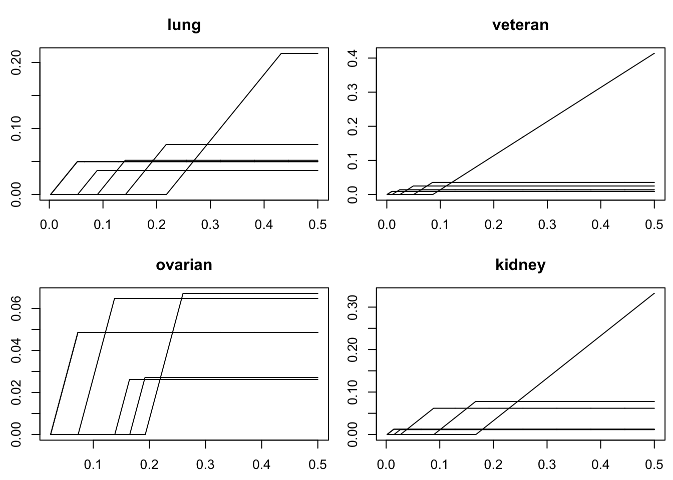
Figure 1: Monotonic splines $\bm{\mathcal{Z}}_{\alpha}$ used to model log cumulative hazards and obtain beta conditional distributions. After differentiation $D_{t}\bm{\mathcal{Z}}_{\alpha}$, we have delta functions $\delta_{j}(t)$ for $J=5$ partitions. Partition boundaries $s_{j}$ were obtain based on the quantiles of event times. Study times are scaled to interval $\left[0,0.5\right]$ and plotted on the x-axis.

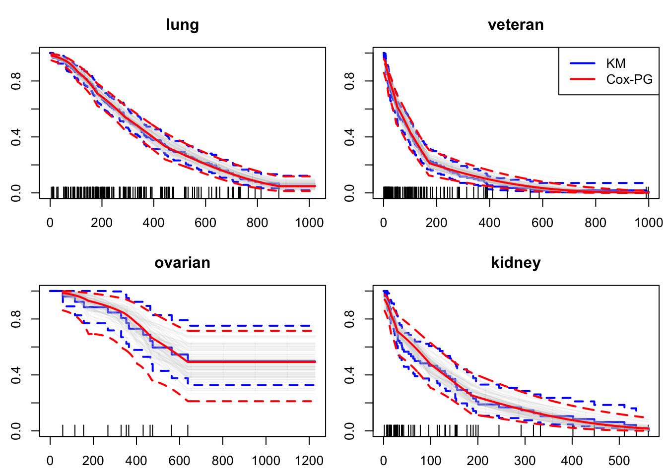
Figure 2: Kaplan-Meier estimates and Cox-PG posterior means of survival curves for 4 datasets. The 0.95 bands are plotted for both methods with dashed lines. Event (death) time ticks are plotted on the x-axis. A sample of 100 Cox-PG posterior draws are plotted in transparent gray to demonstrate variability and monotonicity of MCMC draws. Original study times are plotted on the x-axis.

5 Simulation study

Following the example of Brilleman et al. 2021, we simulate Weibull PH models $\mathbf{m}_{i}^{\top}\bm{\eta}=\alpha(t_{i})+x_{1i}\beta_{1}+x_{2i}\beta_{2}$ where $\alpha(t_{i})=\log(0.1)-2.0+1.5\log\left(t_{i}\right)$ is the baseline log cumulative hazard and $X_{1i}\sim\mathrm{U}(0,1)$, $X_{2i}\sim\operatorname{Ber}(p=0.5)$. We set regression coefficients as $\beta_{1}=1$ and $\beta_{2}=0.5$ and used two settings to show high and low censoring rate. For a high rate of censoring, we drew independent censoring times from $\text{Weibull}\{a=1.5,\sigma=\exp(3)\}$ following pdf $f(x)=(a/\sigma)(x/\sigma)^{a-1}\exp\left(-(x/\sigma)^{a}\right)$. For a low censoring rate, we drew censoring times from $\text{Weibull}\{a=1.5,\sigma=\exp(4)\}$. In addition, we looked at two modest sample size settings, small sample size ($N=50$) and large sample size ($N=100$), resulting in four cases of censoring and sample size combinations. For each case, we simulated $250$ replicates and drew $5000$ MCMC samples, with $1000$ used for burn-in and thinned to obtain $1000$ posterior samples.

We compare Cox-PG using $J=5$ partitions with the standard Cox model. We observed comparable performance with the Cox procedure with only 5 partitions. Our methods allows us to recover the baseline log cumulative hazard in addition to the regression coefficients. Cox-PG posterior draws and theoretical results allow us to conduct valid Bayesian inference on the nonparametric hazard object and coefficients without relying on large sample theory. In the $N=100$ sample settings our competing methods yield similar results (see Table 1 & 2). We used a simple intuitive procedure for spline construction, though tuning number of basis functions $J$ and knot selection, can result in better performance of Cox-PG. In addition, informative priors can used in low sample settings to incorporate domain information into modeling. In summary, naive knot selection with only $5$ splines already performs comparably to Cox PH regression under the modest sample size of $N=100$.

In Figure 3, we plot Cox-PG posterior mean estimates of $\alpha(t)$ for $250$ replicates compared with the truth. Figure 3 can be interpreted similarly to a mean square error (MSE), though end points differ between replicates. The low censoring and large sample setting had the most accurate estimates, where we observed the most variability in the high censoring and small sample setting. The Gibbs sampler accurately captured the shape of the baseline hazard distribution while enforcing for monotonicity in all four cases. Inference on the log cumulative hazard can be conducted following the examples of Section 4.

Table 1: Mean coefficient estimates across replicates and mean squared error (MSE). Cox-PG sampler and Cox regression were compared in four settings of censoring rates and finite samples. Data was simulated using coefficients $\beta_{1}=1$ and $\beta_{2}=0.5$. High and low censoring are given by $\mathrm{Weibull}(1.5,e^{3})$ and $\mathrm{Weibull}(1.5,e^{4})$ respectively.

	mean ${\beta}_{1}$		mean ${\beta}_{2}$		$\text{MSE}(\beta_{1})$		$\text{MSE}(\beta_{2})$
	Cox-PG	Cox	Cox-PG	Cox	Cox-PG	Cox	Cox-PG	Cox
$\mathrm{Weibull}(1.5,e^{4})$ $N=100$	1.093	1.029	0.564	0.535	0.169	0.150	0.060	0.052
$\mathrm{Weibull}(1.5,e^{4})$ $N=50$	1.153	1.055	0.59	0.537	0.435	0.369	0.163	0.129
$\mathrm{Weibull}(1.5,e^{3})$ $N=100$	1.057	1.003	0.552	0.523	0.210	0.190	0.064	0.055
$\mathrm{Weibull}(1.5,e^{3})$ $N=50$	1.060	0.960	0.567	0.516	0.529	0.463	0.194	0.155

Table 2: Coverage rate (CR) based on 0.95 intervals and mean coverage-interval length (CL).

	$\text{CR}(\beta_{1})$		$\text{CR}(\beta_{2})$		$\text{CL}(\beta_{1})$		$\text{CL}(\beta_{2})$
	Cox-PG	Cox	Cox-PG	Cox	Cox-PG	Cox	Cox-PG	Cox
$\mathrm{Weibull}(1.5,e^{4})$ $N=100$	0.924	0.940	0.916	0.928	1.519	1.52	0.871	0.868
$\mathrm{Weibull}(1.5,e^{4})$ $N=50$	0.916	0.948	0.908	0.94	2.229	2.228	1.273	1.269
$\mathrm{Weibull}(1.5,e^{3})$ $N=100$	0.948	0.96	0.968	0.972	1.715	1.711	0.980	0.980
$\mathrm{Weibull}(1.5,e^{3})$ $N=50$	0.928	0.952	0.888	0.94	2.523	2.518	1.456	1.438

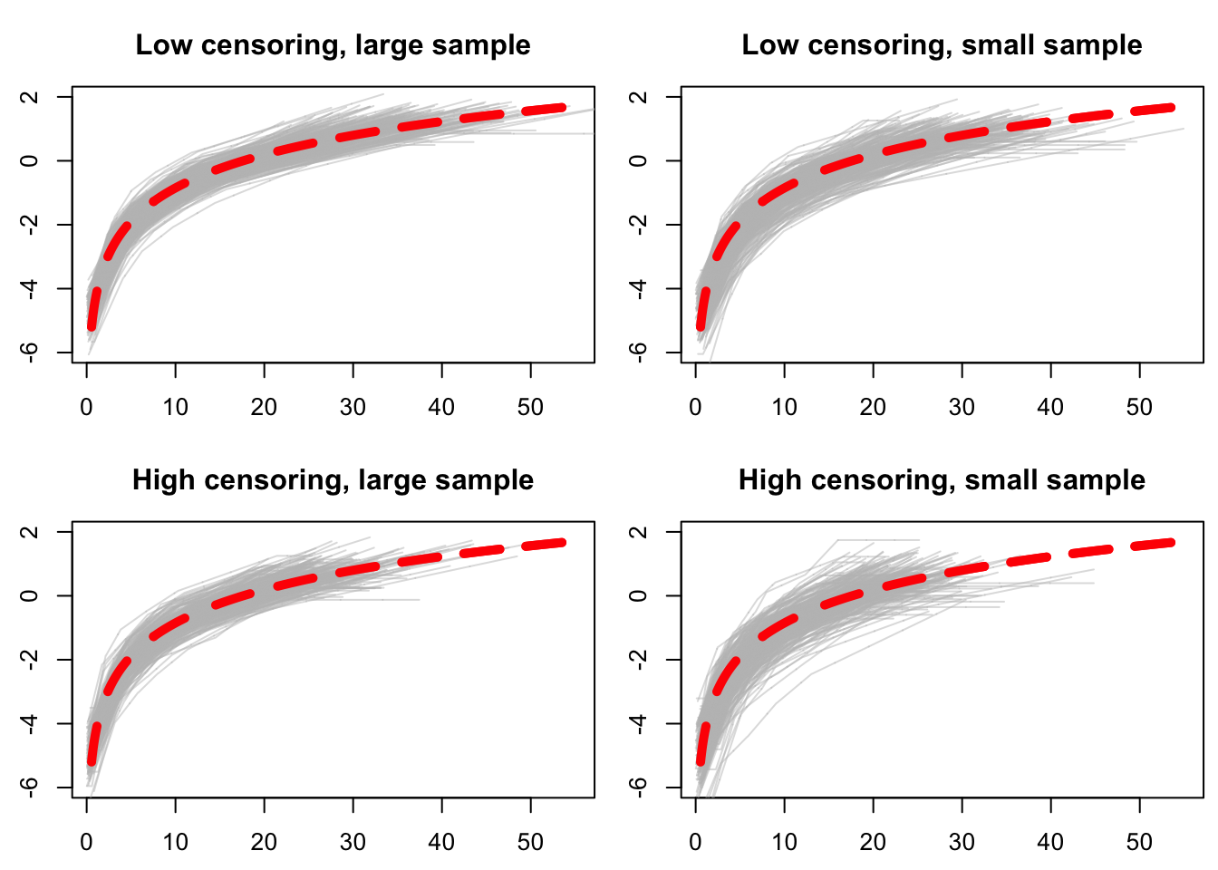
Figure 3: Cox-PG posterior mean estimates of baseline log cumulative hazard $\alpha(t)$. The true log cumulative hazard is plotted with red dashed lines.

6 Discussion

As sample size increases, $n_{\alpha,j}$ increases leading to $v_{j}/u_{\alpha,j}\rightarrow 1$ from the left. This leads to slow mixing of the MCMC by causing $u_{\alpha,j}^{(n-1)}\approx u_{\alpha,j}^{(n)}$. We can decrease $n_{\alpha,j}$ by increasing the number of partitions $J$. However, this results in a high dimensional truncated Gaussian, where the SIR algorithm is inefficient. The Hamiltonian Monte Carlo approach of Pakman & Paninski 2014 that uses the Hamiltonian canonical transformation to sample truncated Gaussian is a promising next step to improve the Cox-PG algorithm.

The link between Cox models and logistic regression is well known, with relative risks being equal to odds ratios in rare event settings. Because Cox models admits a local Poisson representation, we may reformulated Cox models as local negative binomial processes with a vague gamma mixture. These local negative binomial processes are in fact rare event logistic regressions with an appropriate offset term. This allows access to Bayesian computational and inferential tools for logistic regression that can be deployed in survival settings. Of these tools, we use Polya-gamma auxiliary variables that further allows inference to be facilitated through Gaussian sampling. We pair the PG variable with sufficiently reduced beta slice auxiliary variables to address the density corresponding to the baseline hazard in a computationally efficient procedure. We slice sample into sliced inverse regression using these beta auxiliary variables. Together, beta and PG auxiliaries reduce the inference to truncated Gaussian sampling on a half space.

These techniques serve as a foundation for Cox model Bayesian inference. It may be possible to show geometric ergodicity under flat priors using proof strategies from Wang & Roy 2018b. Many multilevel models are straight forward modifications. In addition, we are able to present conditions for convergence. This would allow us to construct succinct Markov chains to traverse many varieties of Bayesian survival models.

References

- (1)
- Aalen (1978) Aalen, O. (1978), ‘Nonparametric inference for a family of counting processes’, The Annals of Statistics pp. 701–726.
- Aalen et al. (2008) Aalen, O., Borgan, O. & Gjessing, H. (2008), Survival and event history analysis: a process point of view, Springer Science & Business Media.
-
Bhattacjarjee (2016)
Bhattacjarjee, S. (2016), tmvnsim:
Truncated Multivariate Normal Simulation.
R package version 1.0-2.
https://CRAN.R-project.org/package=tmvnsim - Blanchet et al. (2022) Blanchet, J., Murthy, K. & Si, N. (2022), ‘Confidence regions in wasserstein distributionally robust estimation’, Biometrika 109(2), 295–315.
- Boyd & Vandenberghe (2004) Boyd, S. P. & Vandenberghe, L. (2004), Convex optimization, Cambridge university press.
- Brilleman et al. (2021) Brilleman, S. L., Wolfe, R., Moreno-Betancur, M. & Crowther, M. J. (2021), ‘Simulating survival data using the simsurv r package’, Journal of Statistical Software 97, 1–27.
- Chen et al. (2006) Chen, M.-H., Ibrahim, J. G. & Shao, Q.-M. (2006), ‘Posterior propriety and computation for the cox regression model with applications to missing covariates’, Biometrika 93(4), 791–807.
-
Choi & Hobert (2013)
Choi, H. M. & Hobert, J. P. (2013), ‘The Polya-Gamma Gibbs sampler for Bayesian logistic regression is
uniformly ergodic’, Electronic Journal of Statistics 7(none), 2054 – 2064.
https://doi.org/10.1214/13-EJS837 - Cong et al. (2017) Cong, Y., Chen, B. & Zhou, M. (2017), ‘Fast simulation of hyperplane-truncated multivariate normal distributions.’, Bayesian Analysis 12(4).
- Cox (1972) Cox, D. R. (1972), ‘Regression models and life-tables’, Journal of the Royal Statistical Society: Series B (Methodological) 34(2), 187–202.
- Cui et al. (2021) Cui, E., Crainiceanu, C. M. & Leroux, A. (2021), ‘Additive functional cox model’, Journal of Computational and Graphical Statistics 30(3), 780–793.
- Damien et al. (1999) Damien, P., Wakefield, J. & Walker, S. (1999), ‘Gibbs sampling for bayesian non-conjugate and hierarchical models by using auxiliary variables’, Journal of the Royal Statistical Society: Series B (Statistical Methodology) 61(2), 331–344.
- Esscher (1932) Esscher, F. (1932), ‘On the probability function in the collective theory of risk’, Skand. Aktuarie Tidskr. 15, 175–195.
- Geweke (1989) Geweke, J. (1989), ‘Bayesian inference in econometric models using monte carlo integration’, Econometrica: Journal of the Econometric Society pp. 1317–1339.
- Hector & Song (2021) Hector, E. C. & Song, P. X.-K. (2021), ‘A distributed and integrated method of moments for high-dimensional correlated data analysis’, Journal of the American Statistical Association 116(534), 805–818.
- Hothorn et al. (2018) Hothorn, T., Möst, L. & Bühlmann, P. (2018), ‘Most likely transformations’, Scandinavian Journal of Statistics 45(1), 110–134.
- Ibrahim et al. (2001) Ibrahim, J. G., Chen, M.-H. & Sinha, D. (2001), Bayesian survival analysis, Vol. 2, Springer.
- Ildstad et al. (2001) Ildstad, S. T., Evans Jr, C. H. et al. (2001), ‘Small clinical trials: Issues and challenges’.
- Jones (2004) Jones, G. L. (2004), ‘On the markov chain central limit theorem’.
- Jones & Hobert (2001) Jones, G. L. & Hobert, J. P. (2001), ‘Honest exploration of intractable probability distributions via markov chain monte carlo’, Statistical Science pp. 312–334.
- Kalbfleisch (1978) Kalbfleisch, J. D. (1978), ‘Non-parametric bayesian analysis of survival time data’, Journal of the Royal Statistical Society: Series B (Methodological) 40(2), 214–221.
- Kalbfleisch & Prentice (2011) Kalbfleisch, J. D. & Prentice, R. L. (2011), The statistical analysis of failure time data, John Wiley & Sons.
- Kaplan & Meier (1958) Kaplan, E. L. & Meier, P. (1958), ‘Nonparametric estimation from incomplete observations’, Journal of the American statistical association 53(282), 457–481.
- Lee et al. (2018) Lee, W., Miranda, M. F., Rausch, P., Baladandayuthapani, V., Fazio, M., Downs, J. C. & Morris, J. S. (2018), ‘Bayesian semiparametric functional mixed models for serially correlated functional data, with application to glaucoma data’, Journal of the American Statistical Association .
- Li (2018) Li, B. (2018), Sufficient dimension reduction: Methods and applications with R, CRC Press.
- Li (1991) Li, K.-C. (1991), ‘Sliced inverse regression for dimension reduction’, Journal of the American Statistical Association 86(414), 316–327.
- Li (2004) Li, K.-H. (2004), ‘The sampling/importance resampling algorithm’, Applied Bayesian Modeling and Causal Inference from Incomplete-Data Perspectives: An Essential Journey with Donald Rubin’s Statistical Family pp. 265–276.
- Li & Ghosh (2015) Li, Y. & Ghosh, S. K. (2015), ‘Efficient sampling methods for truncated multivariate normal and student-t distributions subject to linear inequality constraints’, Journal of Statistical Theory and Practice 9, 712–732.
- Maatouk & Bay (2016) Maatouk, H. & Bay, X. (2016), A new rejection sampling method for truncated multivariate gaussian random variables restricted to convex sets, in ‘Monte Carlo and Quasi-Monte Carlo Methods: MCQMC, Leuven, Belgium, April 2014’, Springer, pp. 521–530.
- McGregor et al. (2020) McGregor, D., Palarea-Albaladejo, J., Dall, P., Hron, K. & Chastin, S. (2020), ‘Cox regression survival analysis with compositional covariates: application to modelling mortality risk from 24-h physical activity patterns’, Statistical methods in medical research 29(5), 1447–1465.
- McLain & Ghosh (2013) McLain, A. C. & Ghosh, S. K. (2013), ‘Efficient sieve maximum likelihood estimation of time-transformation models’, Journal of Statistical Theory and Practice 7, 285–303.
- Meyer et al. (2018) Meyer, M. C., Kim, S.-Y. & Wang, H. (2018), ‘Convergence rates for constrained regression splines’, Journal of Statistical Planning and Inference 193, 179–188.
- Meyer et al. (2015) Meyer, M. J., Coull, B. A., Versace, F., Cinciripini, P. & Morris, J. S. (2015), ‘Bayesian function-on-function regression for multilevel functional data’, Biometrics 71(3), 563–574.
- Mira & Tierney (2002) Mira, A. & Tierney, L. (2002), ‘Efficiency and convergence properties of slice samplers’, Scandinavian Journal of Statistics 29(1), 1–12.
- Neal (2003) Neal, R. M. (2003), ‘Slice sampling’, The annals of statistics 31(3), 705–767.
- Neelon (2019) Neelon, B. (2019), ‘Bayesian zero-inflated negative binomial regression based on pólya-gamma mixtures’, Bayesian analysis 14(3), 829.
- Nelson (1972) Nelson, W. (1972), ‘Theory and applications of hazard plotting for censored failure data’, Technometrics 14(4), 945–966.
- Nieto-Barajas & Walker (2002) Nieto-Barajas, L. E. & Walker, S. G. (2002), ‘Markov beta and gamma processes for modelling hazard rates’, Scandinavian Journal of Statistics 29(3), 413–424.
- O’Sullivan (1986) O’Sullivan, F. (1986), ‘A statistical perspective on ill-posed inverse problems’, Statistical science pp. 502–518.
- Pakman & Paninski (2014) Pakman, A. & Paninski, L. (2014), ‘Exact hamiltonian monte carlo for truncated multivariate gaussians’, Journal of Computational and Graphical Statistics 23(2), 518–542.
- Polson et al. (2013) Polson, N. G., Scott, J. G. & Windle, J. (2013), ‘Bayesian inference for logistic models using pólya–gamma latent variables’, Journal of the American statistical Association 108(504), 1339–1349.
- Ramsay (1988) Ramsay, J. O. (1988), ‘Monotone regression splines in action’, Statistical science pp. 425–441.
- Roberts & Rosenthal (2004) Roberts, G. O. & Rosenthal, J. S. (2004), ‘General state space markov chains and mcmc algorithms’.
- Ruppert et al. (2003) Ruppert, D., Wand, M. P. & Carroll, R. J. (2003), Semiparametric regression, number 12, Cambridge university press.
- Sinha et al. (2003) Sinha, D., Ibrahim, J. G. & Chen, M.-H. (2003), ‘A bayesian justification of cox’s partial likelihood’, Biometrika 90(3), 629–641.
- Sun et al. (2019) Sun, Q., Zhu, R., Wang, T. & Zeng, D. (2019), ‘Counting process-based dimension reduction methods for censored outcomes’, Biometrika 106(1), 181–196.
- Sy & Taylor (2000) Sy, J. P. & Taylor, J. M. (2000), ‘Estimation in a cox proportional hazards cure model’, Biometrics 56(1), 227–236.
-
Therneau (2023)
Therneau, T. M. (2023), A Package for
Survival Analysis in R.
R package version 3.5-7.
https://CRAN.R-project.org/package=survival - Therneau et al. (2000) Therneau, T. M., Grambsch, P. M., Therneau, T. M. & Grambsch, P. M. (2000), The cox model, Springer.
- Tibshirani (1997) Tibshirani, R. (1997), ‘The lasso method for variable selection in the cox model’, Statistics in medicine 16(4), 385–395.
- Tipping (2001) Tipping, M. E. (2001), ‘Sparse bayesian learning and the relevance vector machine’, Journal of machine learning research 1(Jun), 211–244.
- Tsiatis (2006) Tsiatis, A. A. (2006), ‘Semiparametric theory and missing data’.
- Van der Vaart (2000) Van der Vaart, A. W. (2000), Asymptotic statistics, Vol. 3, Cambridge university press.
- Wand & Ormerod (2008) Wand, M. P. & Ormerod, J. (2008), ‘On semiparametric regression with o’sullivan penalized splines’, Australian & New Zealand Journal of Statistics 50(2), 179–198.
- Wang (1985) Wang, J.-L. (1985), ‘Strong consistency of approximate maximum likelihood estimators with applications in nonparametrics’, The Annals of Statistics pp. 932–946.
- Wang et al. (2022) Wang, T., Ratcliffe, S. J. & Guo, W. (2022), ‘Time-to-event analysis with unknown time origins via longitudinal biomarker registration’, Journal of the American Statistical Association pp. 1–16.
- Wang & Roy (2018a) Wang, X. & Roy, V. (2018a), ‘Analysis of the pólya-gamma block gibbs sampler for bayesian logistic linear mixed models’, Statistics & Probability Letters 137, 251–256.
-
Wang & Roy (2018b)
Wang, X. & Roy, V. (2018b),
‘Geometric ergodicity of Pólya-Gamma Gibbs sampler for Bayesian logistic
regression with a flat prior’, Electronic Journal of Statistics 12(2), 3295 – 3311.
https://doi.org/10.1214/18-EJS1481 - Wienke (2010) Wienke, A. (2010), Frailty models in survival analysis, CRC press.
- Winkelmann (2008) Winkelmann, R. (2008), Econometric analysis of count data, Springer Science & Business Media.
- Wulfsohn & Tsiatis (1997) Wulfsohn, M. S. & Tsiatis, A. A. (1997), ‘A joint model for survival and longitudinal data measured with error’, Biometrics pp. 330–339.
- Zens et al. (2023) Zens, G., Frühwirth-Schnatter, S. & Wagner, H. (2023), ‘Ultimate pólya gamma samplers–efficient mcmc for possibly imbalanced binary and categorical data’, Journal of the American Statistical Association pp. 1–12.
- Zhou et al. (2012) Zhou, M., Li, L., Dunson, D. & Carin, L. (2012), Lognormal and gamma mixed negative binomial regression, in ‘Proceedings of the… International Conference on Machine Learning. International Conference on Machine Learning’, Vol. 2012, NIH Public Access, p. 1343.