Mixup Barcodes: Quantifying Geometric-Topological Interactions between Point Clouds

Abstract

We combine standard persistent homology with image persistent homology to define a novel way of characterizing shapes and interactions between them. In particular, we introduce: (1) a mixup barcode, which captures geometric-topological interactions (mixup) between two point sets in arbitrary dimension; (2) simple summary statistics, total mixup and total percentage mixup, which quantify the complexity of the interactions as a single number; (3) a software tool for playing with the above.

As a proof of concept, we apply this tool to a problem arising from machine learning. In particular, we study the disentanglement in embeddings of different classes. The results suggest that topological mixup is a useful method for characterizing interactions for low and high-dimensional data. Compared to the typical usage of persistent homology, the new tool is sensitive to the geometric locations of the topological features, which is often desirable.

1 Overview

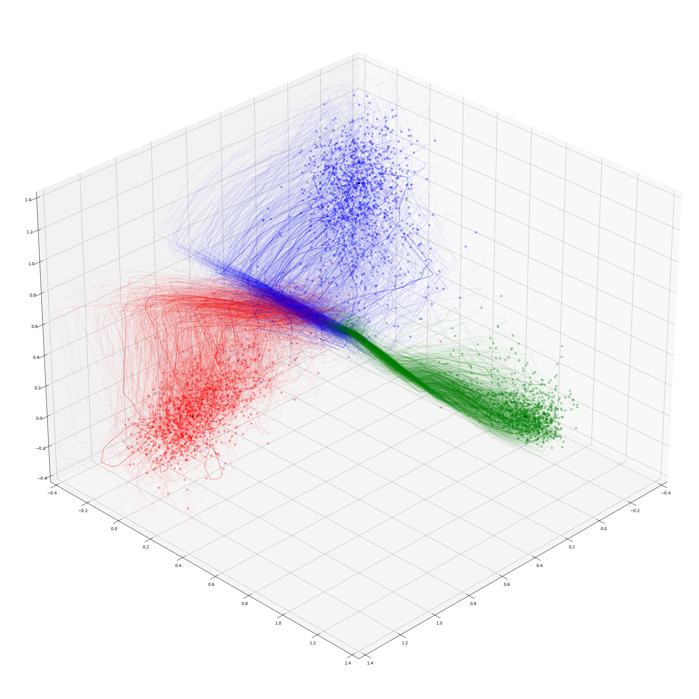
Figure 1: The three point clouds are the predictions produced by a machine learning model for three different classes. The trajectories track the predictions during training. The details of this disentanglement process are hard to visualize clearly even in dimension three, and motivate our topological mixup measurement for data of arbitrary dimension.

Motivated by problems in machine learning, we are interested in characterizing interactions between point clouds – and their evolution over time. In particular, we would like to study how points belonging to different classes are disentangled during the training of a machine learning model. See Figure 1 for a low-dimension version.

More concretely, we consider two labelled point clouds $A$, $B$. To determine the shape of such data and the interactions between them, we will define the notion of topological mixup. More technically, we propose a geometric-topological descriptor called the mixup barcode combining the persistent homology of $A$ and the image persistence of the inclusion of $A$ into $A\cup B$. In practice, we compute the two pieces of information using a new version of ripser, which offers image persistence computations [3], and package them as a single descriptor.

Compared to methods based on comparing standard persistence barcodes, our new descriptor is sensitive to the geometric location of the topological features. We start from a simple illustration in Figures 3 and 3 and later define the concepts in more detail. Later we apply the new method in the context of the disentanglement problem mentioned above.

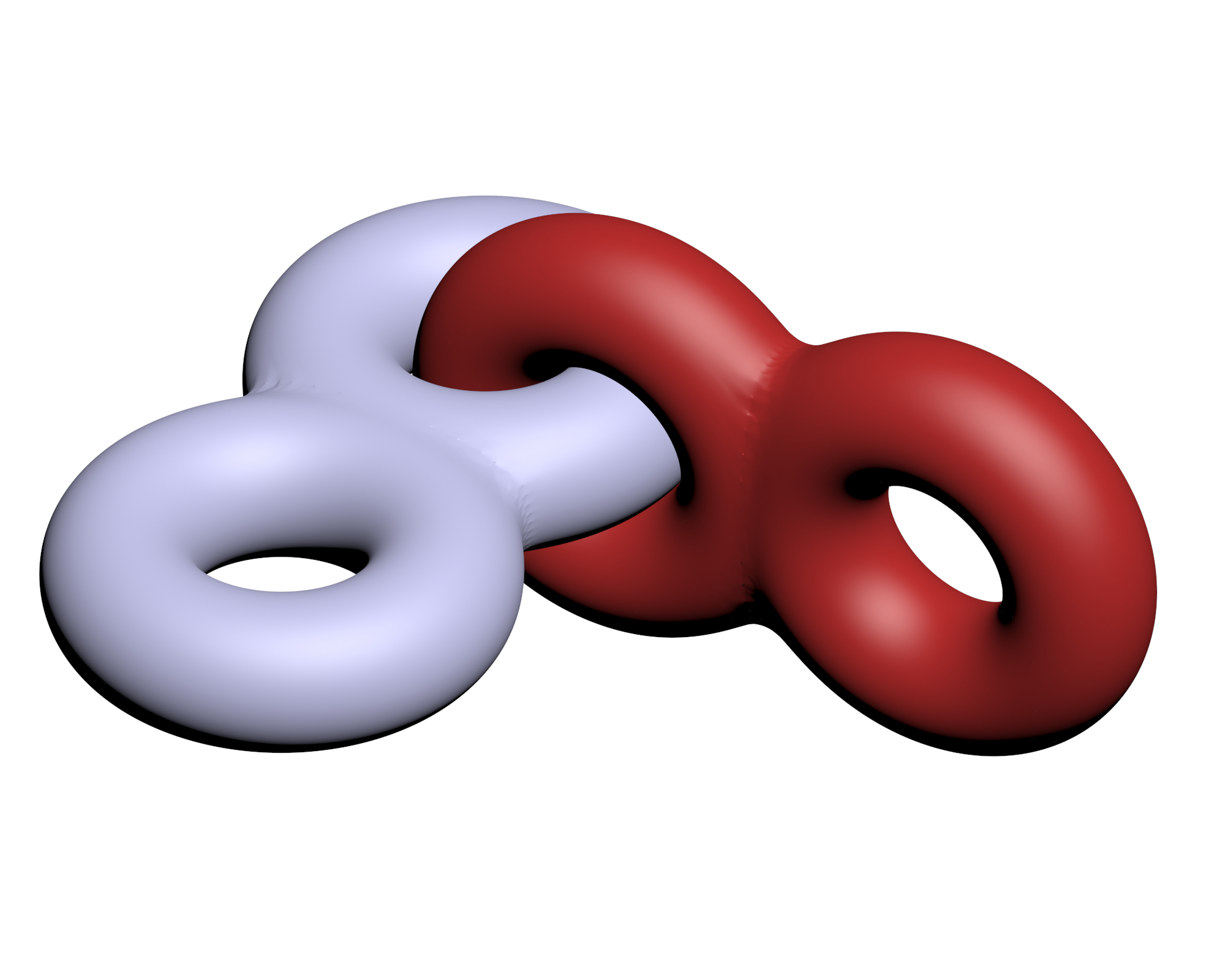
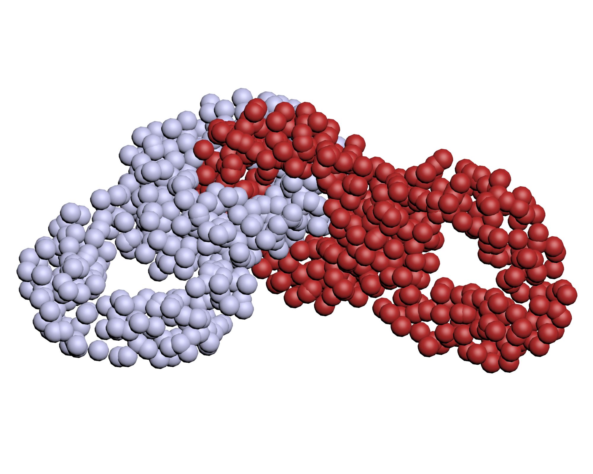
Figure 2: We consider two solid double tori, blue (light) and red (dark). Each has two holes of radius 5. Imagine the blue torus on its own, and then suddenly interlocked with the red one, as depicted. In both situations there are two holes, but the shape has clearly changed. Can we detect this change with topological tools? We sample each torus with 500 points and obtain two point clouds, $A$ (blue) and $B$ (red).

Figure 3: From top to bottom, we show the Vietoris–Rips persistence barcodes for $A$, $A\cup B$, and the mixup barcode for $A\hookrightarrow A\cup B$. From left to right, the barcodes in degree $0$ and $1$, plus an extra closeup of the top part of the latter. The degree 1 barcodes for $A$ and $A\cup B$ each show two long bars (visible in the closeup), corresponding to the two prominent holes (handles) in $A$ and $A\cup B$ respectively. Each of these holes dies at thickening radius $\approx 5$. Comparing these two barcodes, one could mistakenly conclude that there is no interaction between $A$ and $B$. The mixup barcode between $A$ and $B$ offers richer information: the black sub-bar highlights the shortening of the lifetime of a topological feature arising in $A$ when the points from $B$ are added. In this example, the mixup barcode in degree $1$ correctly detects the interlock between the two tori: the long black bar (better visible in the closeup) shows that the prominent hole in $A$ is filled up by $B$.

Contributions. The contributions of this paper include:

1. A topological descriptor called a mixup barcode characterizing interactions between two point clouds.

2. Simple summary statistics quantifying the robustness of these interactions.

3. Software computing and visualizing the above concepts.

4. Experiments using illustrative low-dimensional examples and high-dimensional data coming from machine learning.

2 Motivation

When analyzing data, knowledge of its geometric and topological features comes in handy. However, many datasets arising in practice are high dimensional, making it challenging to inspect these properties. In particular, many high-dimensional problems in modern machine learning can be distilled to computational geometry – although studying topological properties of data is gaining popularity. Motivated by one such problem, we propose a novel geometric-topological tool.

One method for summarising the geometric-topological structure of data is persistent homology, which has found a variety of applications. Typically, it involves computing a persistence diagram, or barcode, which serves as a geometric-topological descriptor of a dataset. Two datasets can then be compared via an appropriate distance between their barcodes – in particular making the comparison translation and rotation invariant. While often useful, this invariance can be a limitation in certain situations. This is especially true when the specific geometric locations of the topological features play an important role.

Standard persistence is celebrated for its stability. In particular, when each point cloud is perturbed only slightly, the descriptor will vary only slightly, and so does the distance between two descriptors. However, persistence is unstable under adding points to a dataset. We will exploit this feature to quantify how the inclusion of new points affects the topology of a point cloud. This way, we will quantify the degree of topological mixup between point clouds. Later we will frame this in terms of image persistent homology.

Application. Equipped with this tool, we consider the disentanglement problem arising in machine learning. We frame it in geometric and topological terms, keeping machine learning details and jargon to a minimum. In short, we work with labelled point clouds and study the sequence of their embeddings performed by a machine learning model. We are additionally interested in how these embeddings evolve during the training of the model. In particular, highly entangled data is believed to be harder to train with.

Intuitively, points with different labels may be initially mixed up – one point cloud could even be surrounded by another. However, the considered models can arbitrarily increase the dimension, so the point clouds can be disentangled. Ideally, each data point with label $i$ is embedded close to its label, namely the $i$-th standard basis vector in $\mathbb{R}^{l}$, where $l$ is the number of unique labels. See fig:trajectories for an illustration of this process. We are interested in quantifying the disentanglement in the last layer and across different layers, and its evolution during training.

Our tool of choice is persistent homology. It has been applied in the context of disentanglement – but in some cases the limitations of standard persistent homology became obvious. For example: if two point clouds are closely entangled, then one or both of them will (likely) exhibit complicated topology. Therefore, simple topology (likely) implies lack of entanglement. However, two point clouds may have complicated topology on their own but be geometrically separated – which is not captured by persistence itself.

We therefore use an extension of persistent homology which allows us to alleviate this problem. We focus on image persistence [8], which gives us more fine grained information about this disentanglement process. It is a natural tool for the job, and recent progress in computing image persistence for point cloud data [3] encouraged us to perform this pilot study.

3 Related work

We briefly review related work in computational geometry, topology and machine learning.

As for the basics on computational topology, recently published books give an excellent overview including applications. In particular, we mention books by: Wang and Dey [9], Carlsson and Vejdemo-Johansson [5], and Virk [22] which is especially recommended to non-mathematical audiences. We focus on work related to image persistence, and on connections between computational geometry and topology with disentanglement problems coming from machine learning.

Image persistence. Regarding computational methods for image persistence, the initial algorithm was proposed by Cohen-Steiner and collaborators [8]. It also includes the kernel and cokernel counterparts which, for simplicity, we ignore. An implementation is available in the first version of Morozov’s Dionysus library, but currently not in the new version. Chaplin and Natarajan have provided another implementation in their new library phimaker. Recently, Bauer and Schmahl proposed a version [3] of the ripser library for image persistence of Vietoris–Rips complexes. We use it in our computations.

Cultrera di Montesano and collaborators [10] have proposed an approach for analyzing the mingling of a small number of 3-dimensional point clouds using image, kernel and cokernel persistence. The underlying idea is similar to ours, although both projects were developed independently. Our focus on combining standard persistence with image persistence barcodes, while theirs is on different types of persistent homology and connections between them. In their persistence computations they use the phimaker library.

Disentanglement in deep neural networks. In machine learning, disentanglement is a broad concept. We are interested in its aspects related to how embeddings corresponding to different classes are separated during the training of a model. Specifically, we focus on a certain type of an artificial neural network. Our initial motivation for this work goes back to a blog post by Olah on ”Neural Networks, Manifolds, and Topology” from 2014 – only now we have appropriate computational tools. Olah, in turn, cites Cayton’s influential report [6] from 2005 on algorithmic aspects of the manifold hypothesis.

Perhaps the fist explicit mention of (manifold) disentanglement in the context of deep learning is in the work of Brahma, Wu and Yiyuan [4]. The work of Zhou and collaborators provides a topological view on disentanglement in the context of machine learning as well as a thorough overview [24]. We refer the reader interested in the machine learning details there, and focus on geometric-topological aspects of the problem. Our experiments are inspired by the work by Naitzat and collaborators [19] and the follow-up by Wheeler and collaborators  [23]. We aim to alleviate some of the shortcomings of these approaches that stem from the limitations of standard persistence.

4 Standard mathematical background

We review basic computational topology concepts in the context of point cloud data. For a more thorough introduction, we recommend the standard textbook [11] by Edelsbrunner and Harer.

Let $P\subset\mathbb{R}^{d}$ be a finite point cloud. We are interested in the shape of the union of Euclidean balls of radius $r\geq 0$ centered at the points in $P$. To approximate this shape we construct the Vietoris–Rips complex of $P$, which we denote as $VR(P;r)$. Being a simplicial complex, it is composed of simplicies, namely points, edges, triangles and their higher-dimensional analogs. It serves as a combinatorial representation of this union of balls.

Homology. Next we compute homology groups of different degrees, denoted $H_{k}(VR(P;r))$. The word homology stems from the fact that cycles that differ by the boundary of a number of higher dimensional simplices are considered equivalent, or homologous. This way, homology groups capture independent cycles in different degrees.

Caveat: interpretation of homology. For shapes embedded in three dimensional space, homology groups in degree $0$, $1$, $2$ are often intuitively interpreted as various types of holes. $H_{0}$ identifies the gaps between distinct parts of an object (i.e. gives information about its connected components); $H_{1}$ identifies tunnels drilled through the space; $H_{2}$ identifies empty voids completely enclosed by the object – think of a closed bottle full of water. Now the caveat: this interpretation only applies in embedding dimension three. Indeed, if the dimension is increased, the water is free to leak out. Voids can be considered regardless of the embedding dimension, but for objects in $\mathbb{R}^{d}$, this intuition is captured by codimension-$1$ homology, namely $H_{d-1}$.

This is an important distinction in the context of our application. Consider two shapes (e.g. thickened point clouds) in a high-dimensional space. Assume that one encloses the other. It is tempting to think that $H_{2}$ provides an obstruction from disentangling these two shapes without crossing – but this only holds in dimension three.

We stress that in our machine learning application the embedding dimension can be increased arbitrarily. This means that any configuration can be disentangled, at least in principle. Still, it is plausible that complicated entanglement makes for harder training [4]. Additionally, computing higher degree homology remains prohibitively inefficient. These two points limit the utility of homology groups. Still, we view homology – and later image persistent homology – as a practical tool for characterizing shapes and their interactions. Our experiments support this claim.

Persistent homology. Varying the radius $r$ from $0$ to $\infty$, we obtain a finite nested sequence called a Vietoris–Rips filtration, namely

$$VR(P;r_{1})\subseteq VR(P;r_{2})\subseteq\cdots\subseteq VR(P;r_{n}),$$ (1)

which in turn allows us to study the evolution of homology groups as the radius changes,

$$H_{k}(VR(P;r_{1}))\rightarrow H_{k}(VR(P;r_{2}))\rightarrow\cdots\rightarrow H_{k}(VR(P;r_{n})).$$ (2)

As the radius $r$ increases, new homology classes are created and subsequently destroyed, i.e. become trivial or merge with an older class. This information can be computed using specialized software packages, such as ripser [2]. It outputs a collection of pairs $(birth_{P}(\gamma),death_{P}(\gamma))$, corresponding to the radii at which a homology class $\gamma$ is born and dies. This pair is called the persistence pair of $\gamma$, alluding to persistence as the lifetime of the class, namely $pers_{P}(\gamma)=death_{P}(\gamma)-birth_{P}(\gamma)$. A collection of persistence pairs is often visualized as a persistence diagram or persistence barcode[13]. One useful summary of a barcode is its total persistence, which is simply the sum of the lengths of all its bars.

We note some technicalities. Throughout the paper we focus on reduced persistent homology, which in this case means we ignore the infinite pair representing the sole surviving connected component. As a consequence, all bars have finite persistence, and the total persistence is a finite number. Also, we take a notational shortcut: when talking about e.g. a topological feature arising in $P$, we technically mean an element of a homology group in the sequence in Equation 2 for a point cloud $P$.

5 Setup for topological mixup

We overview our construction, which is based on the special case of the persistence of images, kernels and cokernels introduced by Cohen-Steiner, Edelsbrunner, Harer and Morozov [8]. We restrict our attention to Vietoris–Rips filtrations of finite point clouds. The computational machinery for image persistence recently proposed by Bauer and Schmahl [3] focuses on Vietoris–Rips filtrations as well. It is however more general: it allows more general maps between two point clouds, whereas we focus on inclusions. Still, we will use this method for computations, since it is currently the most suitable implementation for high-dimensional data. In this section we focus on sketching the mathematical setup, and elaborate on practical computations in Section 6.

We now consider not one but two point clouds, $A,B\subset\mathbb{R}^{d}$. We construct the Vietoris–Rips filtrations of $A$ and $A\cup B$, noting that $VR(A;r_{i})$ is a subcomplex of $VR(A\cup B;r_{i})$ for each $i$. We let $L_{i}=H_{\bullet}(VR(A;r_{i}))$ and $K_{i}=H_{\bullet}(VR(A\cup B;r_{i}))$. By $H_{\bullet}$ we mean simplicial homology in any reasonable degree. The inclusions of simplicial complexes induce maps at homology level, giving rise to the following commutative diagram

$$\centering\setcounter{MaxMatrixCols}{13}\begin{CD}L_{1}@>{}>{}>L_{2}@>{}>{}>\ldots @>{}>{}>L_{i}@>{}>{}>\ldots @>{}>{}>L_{n}\\ @V{v_{1}}V{}V@V{v_{2}}V{}V@V{v_{i}}V{}V@V{v_{n}}V{}V\\ K_{1}@>{}>{}>K_{2}@>{}>{}>\ldots @>{}>{}>K_{i}@>{}>{}>\ldots @>{}>{}>K_{n}\end{CD}\@add@centering$$ (3)

Each horizontal arrow is induced by the inclusion $VR(\ .\ ;r_{i})\hookrightarrow VR(\ .\ ;r_{i+1})$, and each vertical arrow, $v_{i}$, by $VR(A;r_{i})\hookrightarrow VR(A\cup B;r_{i})$.

Image persistence. We will extract the following information from this diagram. Intuitively, given a feature arising in $A$, we would like to know how long it persists in the presence of points from $B$. We set this up as the persistence of the sequence $\operatorname{im}v_{1},\operatorname{im}v_{2},\dots,\operatorname{im}v_{n}$, called image persistent homology [8]. For technical details, we refer the interested reader to [8].

In practice, we will use a version of the ripser software for image persistence. It returns a collection of image persistence pairs of the form $(birth_{A}(\gamma),death_{A\cup B}(v_{i}(\gamma))$, for a homology class $\gamma$ in $L_{*}$. Specifically, $death_{A\cup B}$ is the radius at which $v_{i}(\gamma)$ is destroyed by boundaries arising from $A\cup B$. In a moment, we will introduce a descriptor that combines information coming from standard persistence and image persistence.

Observation 1

Given a homology class $\gamma$ born at $L_{i}$, $death_{A\cup B}(v_{i}(\gamma))\leq death_{A}(\gamma)$.

The above is true, because for each $j\geq i$ there are more boundaries coming from $VR(A\cup B,r_{j})$ than from $VR(A,r_{j})$ that can destroy $\gamma$, but nothing can prolong its life.

Mixup triple. In analogy with standard persistence, we define the mixup triple of a homology class $\gamma$ born at $L_{i}$ as

$$(birth_{A}(\gamma),\,death_{A\cup B}(v_{i}(\gamma)),\,death_{A}(\gamma)).$$ (4)

This triple stores information about the standard and image persistence pairs, which share the birth radii. We clarify that if $v_{i}(\gamma)$ is already dead at $K_{i}$, then $death_{A\cup B}(v_{i}(\gamma))=r_{i}$.

Mixup. We define the topological mixup, or simply mixup, of a homology class $\gamma$ born at $L_{i}$ as the difference of its two lifetimes, namely

$$mixup(\gamma)=(death_{A}(\gamma)-birth_{A}(\gamma))-(death_{A\cup B}(\gamma)-birth_{A}(\gamma)),$$ (5)

which simplifies to:

$$mixup(\gamma)=death_{A}(\gamma)-death_{A\cup B}(v_{i}(\gamma)),$$ (6)

showing that this quantity is nonnegative. We mention it is closely related to kernel persistence, and we focus on image persistence simply because there is software we can use to compute it.

Mixup barcode. We now introduce a topological descriptor, the mixup barcode between $A$ and $B$, meant to characterize interactions between point clouds $A$ and $B$.

The mixup barcode represents a multiset of mixup triples. As a modification of the standard persistence barcode, it allows for a similar visualization while providing additional information. Each bar in the mixup barcode corresponds to a standard persistence bar for $A$ split into:

1. [i]

2. a sub-bar $(b_{A},\,d_{A\cup B})$ (visualized in light color)

3. a sub-bar $(d_{A\cup B},\,d_{A})$ (visualized in black)

The length of the latter is the mixup of the entire bar. We consider a separate mixup barcode for each degree, in practice 0 and 1. See Figure 4 for an example.

Intuitively, the mixup barcode describes how the lifetimes of topological features arising from $A$ are shortened when $A$ becomes polluted or mixed up with points in $B$.

Stability. The mixup barcode is stable under perturbations of $A$ and $B$, simply because standard [7] and image persistence are both stable [8]. It therefore makes sense to track the mixup as $A$ and $B$ change – part of our application is focused on that.

Total mixup. We can now define a simple summary statistic, namely a number quantifying the amount of mixup for the chosen degree (of homology). The total mixup between point clouds $A$ and $B$ is the sum of the mixups for all bars in their mixup barcode. In our visualization, it is simply the sum of the lengths of the black bars. Equivalently, it is the difference between the total persistence of $A$ and the total image persistence of $A\hookrightarrow A\cup B$. We will refer to this quantity as total-mixup$(A,B)$.

Total mixup percentage. To make the measurement scale-invariant, we define mixup percentage of a homology class $\gamma$ born at $L_{i}$ as

$$mixup_{\%}(\gamma)=\frac{mixup(\gamma)}{pers_{A}(\gamma)}=\frac{death_{A}(\gamma)-death_{A\cup B}(v_{i}(\gamma))}{death_{A}(\gamma)-birth_{A}(\gamma)}.$$ (7)

Conveniently this value is between 0 and 1. A mixup bar inherits the mixup percentage from the corresponding homology class.

Given the mixup barcode, we define its total mixup percentage (mean mixup percentage) as the sum (mean) of the mixup percentages over all its bars. Note that the latter variant is between 0 and 1, but is not the ratio of the total mixup and the total persistence. Note that unlike the mixup barcode, this summary is generally unstable.

No matching. In the standard case, computing the distance between persistence barcodes involves finding a minimum-cost bipartite matching between them. This can be a computationally costly step, although efficient shortcuts have been proposed [15]. Importantly, this step is oblivious to the geometric locations of the topological features – so two geometrically distinct features may be matched.

In our setting, we track the two lifetimes of each feature arising in $A$ – no choice needs to be made to combine these two pieces of information. (In Section 6 we elaborate on how we do this done in practice.) The consequences are twofold. First, the algorithmic matching step is circumvented. Second, geometrically unrelated cycles cannot affect the comparison, which is important in some applications.

Sampling. The following observation will prove useful in our experiments.

Observation 2 (Subsampling Property)

Given point clouds $A$, $B$ and $B^{\prime}\subset B$, total-mixup($A,B^{\prime}$) $\leq$ total-mixup($A,B$).

This follows from Observation 1. So while the births of homology classes arising in $A$ are unaffected by $B$, their deaths can only be delayed by using a subsample of $B$. Additionally, subsampling $B$ never destroys the topological signal present in $A$.

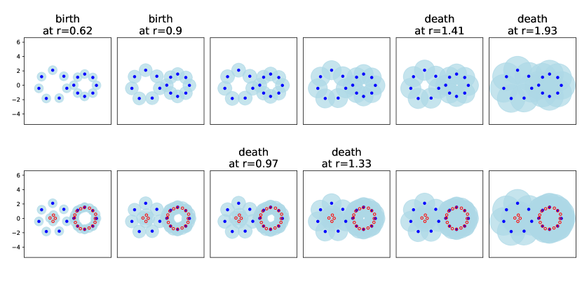
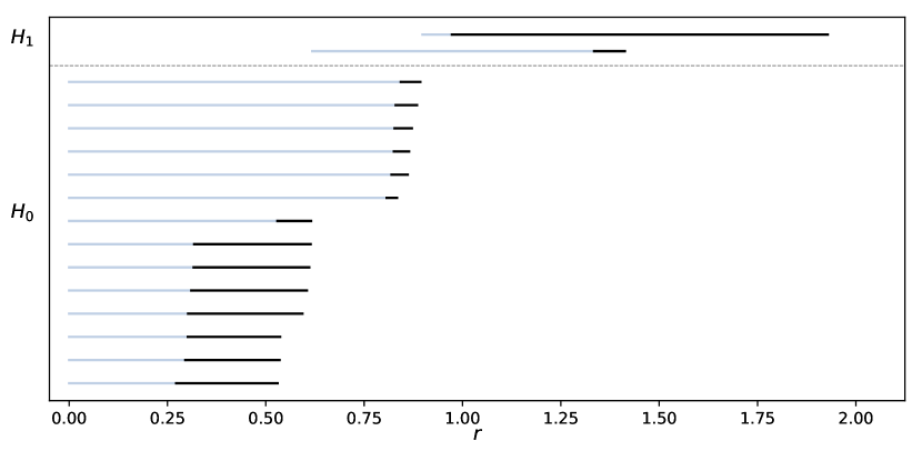
Figure 4: Top: An illustration of our topological mixup construction for $A$ (blue disks) and $B$ (red circles). The two upper rows show the union of growing balls around $A$ and the bottom row for $A\cup B$.
Bottom: The mixup barcodes in degree 1 (top) and 0 (bottom) for the above example. The light bars depict the image persistence, and the black bars the topological mixup.
The larger 1-dimensional cycle on the left is filled in sooner when the red points are included. The points sampling the smaller circle connect sooner via the red point, but this does not significantly affect the death of the smaller 1-dimensional cycle. In particular, note that the smaller cycle does not instantly die. This differentiates the image persistence setup from simply including a homology class into the union of balls with radius $r$ around $A\cup B$. Instead, the role of the balls around the points in $B$ is to help fill in this cycle, potentially quickening its destruction.

6 Implementation

Our software comprises of $\approx 1000$ lines of python code, using numpy to speed up general computations and keras for the machine learning part. We use a modified version of the ripser software for persistence computations. In this section we review some technicalities, including the usage and modifications of ripser. We also comment on how we subsample the data to alleviate some efficiency issues.

6.1 Ripser for image persistence

At the core of our method is the recent extension of the ripser package [2] which computes image persistence [3]. It is currently the only method for image persistence optimized for Vietoris–Rips complexes. To calculate the mixup barcode of data, we introduced modifications to the software.

Standard ripser accepts a pairwise distance matrix (among other formats) and returns the standard persistence barcode. The image persistence version of ripser accepts two distance matrices, $L$, $K$. They represent two finite metric spaces over the same underlying set connected by a nonexpanding map. This is a more general setting than ours and we need to convert our input to this format. We must prevent the points in $B$ from interfering with the persistence computation for $A$, while still emulating the inclusion of $A$ into $A\cup B$.

Assuming that the cardinality of $A$ and $B$ are respectively $n$ and $m$, both matrices will have size $(n+m)\times(n+m)$. $K$ is just the pairwise distance matrix of $A\cup B$. We define $L$ as:

$$L_{ij}=\begin{cases}d(A_{i},A_{j})&\text{if }1\leq i,j\leq n\\ 0&\text{if }i=j\\ D+2\epsilon&\text{if }i\neq j\text{ and }i,j>n,\end{cases}$$ (8)

for $D=\max_{i,j}K_{ij}$ and a reasonable $\epsilon>0$. To be explicit, this is how we call ripser to get standard persistence: ripser-image L --threshold D+epsilon and image persistence: ripser-image K --subfiltration L --threshold D+epsilon.

In postprocessing, we excise undesirable information by filtering out the infinite bars returned by ripser (they correspond to bars with death exceeding $D+\epsilon$). We have to be especially careful in degree $0$. This is because every point in $A\cup B$ is a generator of a zeroth homology group – and we are only interested in tracking the topological features arising in $A$. In this case filtering out the infinite bars excises all components arising from $B$, since their death exceeds $D+\epsilon$ by construction. One extra thing removed is the single infinite bar coming from $A$, which we meant to discard anyway.

Combining barcodes. To construct the mixup barcode, we run ripser twice: once for standard persistence and once for image persistence. The two resulting barcodes are then combined. Mathematically, there is no choice to be made at this step, as we track each feature arising in one of the inputs. In practice, we need to find an injection between the finite parts of these barcodes. Each remaining standard bar $(b,d)$ is augmented with an artificial pair $(b,b)$. In degree 1, finding this injection is straightforward: thanks to stability, the input matrices can be slightly perturbed to ensure uniqueness of births. We can therefore unambiguously combine the pairs by their birth via sorting. In degree zero all components are born at radius zero, which requires extra work. Handling higher degrees would require more significant changes.

Modifications of ripser. We modified ripser to enable combining barcodes in degree zero. In the original implementation, all bars are assigned a birth time of $0$, making them impossible to differentiate. To resolve this, we allow nonzero values on the diagonal of the distance matrices. Specifically we set the $i$-th diagonal value to $-i$, representing the formal birth times of the connected components. Additionally, we updated the set-union data structure [20] to take this information into account.

These modifications allow us to identify bars in degree zero by their unique birth values. With this information, we can unambiguously combine the two barcodes as we did for higher degrees. In the resulting mixup barcode, the births are reverted to zero, so the choice of diagonal entries does not affect the resulting mixup barcode.

If the input matrix has zeros on the diagonal, the modified ripser returns the same results as the original. However, we had to forgo the union-by-rank optimization [20], increasing the expected and worst-case complexity of computing persistence in degree zero. This is an acceptable trade-off, since the overall computation is heavily dominated by persistence in higher degrees. We also added support for binary-encoded raw input matrices, allowing for fast and seamless data exchange from python using numpy arrays (reading and writing text files was the bottleneck for computations in degree 0).

6.2 Subsampling

Computing image persistence turns out to be generally slower than computing standard persistence for data of similar size and complexity [3]. In particular, in our case increasing the size of point set $B$ tends to degrade performance.

To alleviate this, we reduce the size of data – in particular the size of the point set $B$. The Subsampling Property (obs:subs) tells us that subsampling $B$ is quite safe.

We use the k-medoids algorithm [14], the long lost sibling of the popular k-means clustering [17]. Unlike k-means, it ensures that the cluster centers belong to the input point cloud, so we can indeed use it for subsampling. It was used in a similar context by Li and collaborators [16].

We briefly explain our rationale for using a centroid-based clustering, as opposed to, e.g. taking a uniform random subsample of size $k$. First, it is not crucial to carefully represent the shape of the points in $B$, since their topology has no bearing on the result. Second, we wish to preserve some of the outliers. Indeed, even a single point in $B$ surrounded by points in $A$ may have a large impact on the topological mixup between $A$ and $B$.

7 Machine learning setup

We focus on a popular machine learning model, namely a type of an artificial neural network [1] often called the multi-layer perceptron (MLP). It is perhaps the simplest deep learning method, and we view it in the context of a classification task. Note that, contrary to a popular belief, models based solely on MLPs can achieve state of the art performance on challenging tasks [21].

The goal is to train a model which will reliably predict the correct labels of previously unseen vectors. The training uses data encoded as vectors, along with their correct integer labels. Assuming there are $l$ unique labels, label $j$ is encoded as the $j$-th standard basis vector in $\mathbb{R}^{l}$.

This particular model performs computations in layers: the output of the current layer is the input to the next layer. The output of the last layer is interpreted as the prediction vector. The $i$-th layer can be viewed as a function $L_{i}:\mathbb{R}^{n}\to\mathbb{R}^{m}$, $L_{i}(v)=f_{i}(W_{i}v)$, where $W_{i}$ is a real matrix. Except for the first and last layer, the dimensions $n,m$ can be freely configured but remain fixed during training. The entries of these matrices serve as trainable parameters and are initialized randomly.

The function $f_{i}$ is a component-wise nonlinear function, typically called an activation function. Nowadays, a common choice is the ReLU [12, 18] function, which simply returns $max(0,x)$ at each coordinate. For simplicity, we will use the identity function as the activation for the last layer.

In more geometric terms, each layer performs a linear transformation followed by a projection onto the positive orthant of $\mathbb{R}^{m}$, for some $m$.

Another important choice is the loss function. It evaluates the quality of predictions against the correct labels. The training aims at minimizing this function with respect to the parameters. We use the once-standard mean squared error loss. Its geometric counterpart is the squared Euclidean distance, which we now use when computing the mixup barcodes.

Model. We use a simple 5-layer MLP, yielding embedding dimensions $512,256,128,10$ and $L$, where $L$ depends on the number of considered labels (in our case 3 or 10). The model has $565,248+10L$ trainable parameters (weights).

8 Experiments

We present several experiments in the context of machine learning. The main goal is to highlight the usefulness of the new methodology – especially in comparison to existing applications of standard persistent homology.

Goals. In our experiments we are interested in the embeddings performed by each layer of the model. More precisely, we consider the computation performed by the $i$ initial layers of the model, namely $M_{i}=L_{i}\circ L_{i-1}\circ...\circ L_{1}$. Given a single input vector $v$, we view $(M_{i}(v))_{i}$ as a sequence of embeddings of $v$. Extending this to the entire input point cloud, we get a sequence of point clouds – which additionally change as training progresses. This is what Figure 1 visualizes for the last layer of a model.

We would like to study how these point clouds disentangle – both when passed from one layer to another, and also as training progresses. We characterize this process through the lens of topological mixup.

Note that the intermediate embedding dimensions can be high – and can exceed the dimension of the input data, meaning that any tangle can – in principle – be untangled. Still, complicated entanglement is hypothesised to correlate with training difficulties [24].

8.1 Datasets

We will be using two datasets. We train the model on the test data. We use test images in our experiments, due to their smaller size and larger number of outliers in predictions. For efficiency reasons, whenever we compute the mixup barcode in degree 1, we subsample $A$ with 500 points and $B$ with 100 points. We select a single subsample for all timesteps and layers. In degree 0, we use all available points. We treat the datasets as a finite labelled point cloud in $X\subset\mathbb{R}^{d}$. By $X_{i}$ we mean class $i$ of dataset $X$, namely the subset of points with label $i$.

MNIST. This is a standard dataset, containing 60,000 grayscale images of size $28\times 28$ depicting handwritten decimal digits. It is a heavily preprocessed version of real-world images, so that the Euclidean distance between two images closely corresponds to their perceptual dissimilarity. For this reason, representing the images as a (labelled) point cloud in $\mathbb{R}^{784}$ yields a faithful representation of the data. It comes split into 50,000 training images, and 10,000 test images. We normalize the vectors so that the values are between 0 and 1. The model achieves 99% test accuracy when trained and tested on the images with labels 0,1 and 2, which we then use for our experiments. These are images of handwritten zeros, ones and twos. We know it managed to disentangle the data well from the visualization in Figure 1, so we expect to see low mixup at the end of training. We are however curious about the higher-dimensional embeddings coming from the remaining layers.

CIFAR10. Another standard dataset, containing 50,000 colorful photos of size $32\times 32$ depicting various objects, animals etc. We treat this data as a (labelled) point cloud in $\mathbb{R}^{3072}$, but the Euclidean distance fails to capture the perceptual similarity. Based on this, we expect to see more significant entanglement between different classes. The model is not powerful enough for this data, and achieves only 76% test accuracy when trained and tested the images with labels 0,1 and 2. These are images of airplanes, cars and birds. We expect it to fail to disentangle the data, especially differentiating between airplanes and birds may be hard due to similar backgrounds.

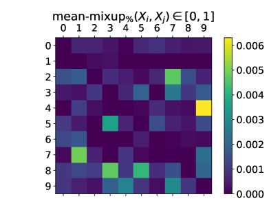
Figure 5: Left: The mean mixup percentage between all pairs of MNIST classes. Most values are low, as expected due to linear separability. Right: The mixup barcode between fours and nines which achieve the greatest mixup. Many bars with small – but positive – mixup suggest that the two point clouds have a shallow overlap – which curiously involves most of the points with label 4.

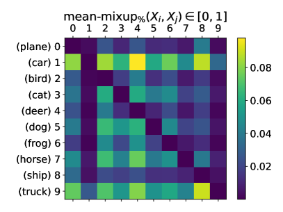
Figure 6: Left: The mean mixup percentage between all pairs of CIFAR10 classes. Note that the values are generally an order of magnitude higher than for the other dataset, with the highest value of 0.09 between classes 1 (airplane) and 4 (deer). Right: The mixup barcode between classes 1 and 4, suggesting a more robust overlap than we saw in the other dataset.

8.2 Entanglement in raw data

While our primary focus is on neural networks, we mention a fact regarding the raw MNIST data. We mention this because previous studies considered the disentanglement of different classes of this dataset [23]. It is however easy to check that the classes are pairwise linearly separable, perhaps with a few outliers. It is therefore unlikely that the pairs of point clouds are entangled. We therefore start from verifying that despite complicated topology, the topological mixup (which we use as a proxy for entanglement) is typically low in this case.

We compute the mean percentage mixup in degree 0 for all pairs of classes of examples, namely for $A=X_{i}$ and $B=X_{j}$ for all $0\leq i,j<10$. The results for MNIST and CIFAR10 are in Figures 5 and 6. As expected, CIFAR10 exhibits greater mixup, often by an order of magnitude. The highest value is between images of fours and nines, which in hindsight makes sense. Note the asymmetry – the mixup between nines and fours is much lower.

8.3 Disentanglement across layers

We study the disentanglement across all layers of the network and its evolution as training progresses. More specifically we compute the total mixup percentage for each: training step, layer ($1-5$), label ($1-3$), degree ($0,1$). Specifically, for label $i$, we compute the mixup barcode between $A=X_{i}$ and $B=X\setminus X_{i}$, take its total mixup percentage. We plot the maximum of this quantity for the three labels. See Figures 7 and 8 for a direct visualization of the results for the MNIST and CIFAR datasets. In particular, the plot for the last layer (closest to the viewer) characterizes the disentanglement during training visualized for MNIST in Figure 1. It is interesting to see that the mixup is initially so low in the early layers – despite the random initialization of the linear transformations. This makes sense, since the data is simple and the embedding dimension is relatively high (512). However, there is much more mixup in later layers, which we attribute to the lower embedding dimension (256,128,10). At the end of the training the mixup is close to 0 for all layers – which we interpret as a successful disentanglement of the three point clouds. This is consistent with our visualization. The mixup in degree 1 is an order of magnitude lower in degree 0.

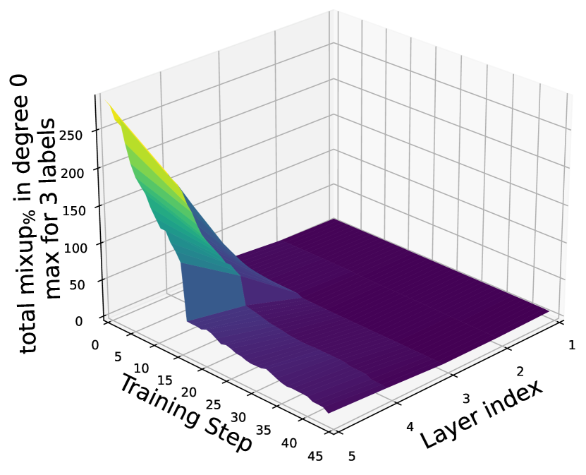
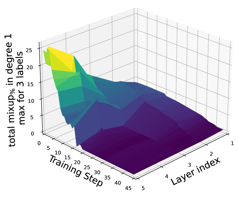
Figure 7: We consider the maximum over the total percentage mixups among the 3 labels. The plot is for the MNIST dataset, in degree 0 (left) and degree 1 (right). It depicts how the mixup changes across layers and through successive training iterations.

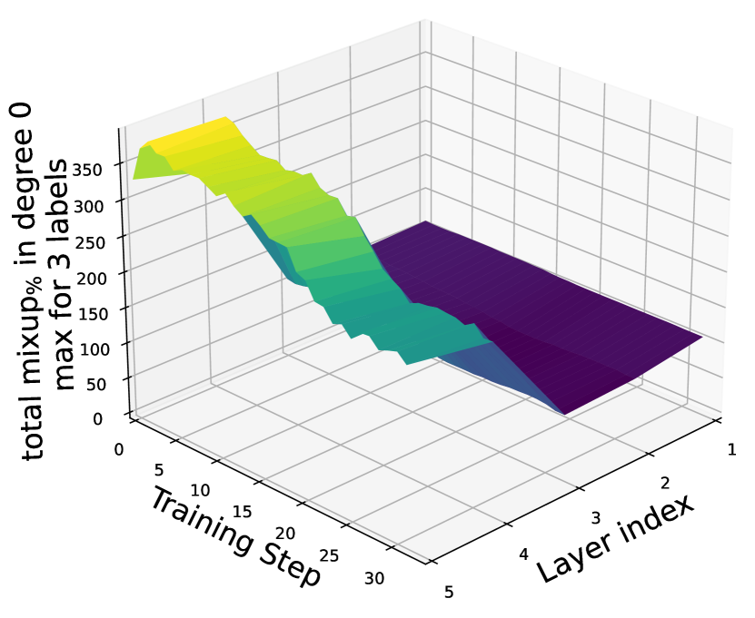
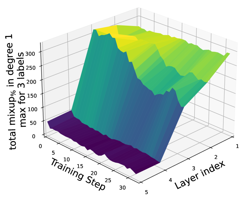
Figure 8: We repeat the experiments from fig:mnist-mixup-over-time for the CIFAR dataset. Note that in general the mixup is much higher for CIFAR as compared to MNIST.

As expected, for the CIFAR dataset, the mixup is overall much higher. As training progresses the mixup decreases, as one would expect, but never goes to zero. In fact the final mixup for CIFAR is comparable to the initial mixup for MNIST. This is consistent with the lower accuracy of the model for the CIFAR dataset compared to the other dataset. Also, we point out that the mixup in the initial layer is high, despite the high dimensionality of this embedding, namely $512$. This likely has to do with the relatively high mixup we saw in the raw data. In degree 1 the high mixup present in early layers drops quickly in later layers. One could hypothesise that the data has interesting large-scale topological structure in the high-dimensional embedding which is destroyed when the dimension is reduced.

9 Discussion

We presented a simple geometric-topological descriptor called a mixup barcode, and its summary statistics. They can be used to characterize the robustness of the interactions between point cloud data. We think the presented examples and experiments show the method is promising.

In particular, the total mixup percentage allowed us to track the disentanglement process across layers of a machine learning model as training progressed. The results align with what we know about the data and its behaviour – but also prompted some new questions.

Currently the main limitation is related to the efficiency degradation when the size of the second dataset increases. However, the software for image persistence computations we adapted, ripser [3], is new and we expect further improvements. Hopefully this work helps motivate development of this type of software.

Overall, our methodology complements the standard persistent homology pipeline, and is tailored for situations where the geometric locations of topological features are important.

References

- [1] Shunichi Amari. A theory of adaptive pattern classifiers. IEEE Transactions on Electronic Computers, EC-16(3):299–307, 1967. \hrefhttps://doi.org/10.1109/PGEC.1967.264666 \pathdoi:10.1109/PGEC.1967.264666.
- [2] Ulrich Bauer. Ripser: efficient computation of vietoris–rips persistence barcodes. Journal of Applied and Computational Topology, 5(3):391–423, 2021.
- [3] Ulrich Bauer and Maximilian Schmahl. Efficient computation of image persistence. In 39th International Symposium on Computational Geometry (SoCG 2023). Schloss Dagstuhl-Leibniz-Zentrum für Informatik, 2023.
- [4] Pratik Prabhanjan Brahma, Dapeng Wu, and Yiyuan She. Why deep learning works: A manifold disentanglement perspective. IEEE Transactions on Neural Networks and Learning Systems, 27(10):1997–2008, 2016. \hrefhttps://doi.org/10.1109/TNNLS.2015.2496947 \pathdoi:10.1109/TNNLS.2015.2496947.
- [5] Gunnar Carlsson and Mikael Vejdemo-Johansson. Topological Data Analysis with Applications. Cambridge University Press, 2021. \hrefhttps://doi.org/10.1017/9781108975704 \pathdoi:10.1017/9781108975704.
- [6] Lawrence Cayton. Algorithms for manifold learning. eScholarship, University of California, 2005.
- [7] David Cohen-Steiner, Herbert Edelsbrunner, and John Harer. Stability of persistence diagrams. In Proceedings of the twenty-first annual symposium on Computational geometry, pages 263–271, 2005.
- [8] David Cohen-Steiner, Herbert Edelsbrunner, John Harer, and Dmitriy Morozov. Persistent homology for kernels, images, and cokernels. In Proceedings of the twentieth annual ACM-SIAM symposium on Discrete algorithms, pages 1011–1020. SIAM, 2009.
- [9] Tamal Krishna Dey and Yusu Wang. Computational Topology for Data Analysis. Cambridge University Press, 2022. \hrefhttps://doi.org/10.1017/9781009099950 \pathdoi:10.1017/9781009099950.
- [10] Sebastiano Cultrera di Montesano, Ondřej Draganov, Herbert Edelsbrunner, and Morteza Saghafian. Persistent homology of chromatic alpha complexes. arXiv preprint arXiv:2212.03128, 2022.
- [11] Herbert Edelsbrunner and John Harer. Computational topology: an introduction. American Mathematical Soc., 2010.
- [12] Kunihiko Fukushima. Visual feature extraction by a multilayered network of analog threshold elements. IEEE Transactions on Systems Science and Cybernetics, 5(4):322–333, 1969. \hrefhttps://doi.org/10.1109/TSSC.1969.300225 \pathdoi:10.1109/TSSC.1969.300225.
- [13] Robert Ghrist. Barcodes: the persistent topology of data. Bulletin of the American Mathematical Society, 45(1):61–75, 2008.
- [14] Leonard Kaufman and Peter J. Rousseeuw. Partitioning around medoids (program pam). In Wiley Series in Probability and Statistics, pages 68–125. John Wiley & Sons, Inc., Hoboken, NJ, USA, 1990. Retrieved 2021-06-13. \hrefhttps://doi.org/10.1002/9780470316801.ch2 \pathdoi:10.1002/9780470316801.ch2.
- [15] Michael Kerber, Dmitriy Morozov, and Arnur Nigmetov. Geometry Helps to Compare Persistence Diagrams. ACM Journal of Experimental Algorithmics, 22(1):1–20, 2017. Published September 18, 2017. \hrefhttps://doi.org/10.1145/3064175 \pathdoi:10.1145/3064175.
- [16] Lei Li, Linda Yu-Ling Lan, Lei Huang, Congting Ye, Jorge Andrade, and Patrick C Wilson. Selecting representative samples from complex biological datasets using k-medoids clustering. Frontiers in Genetics, 13:954024, 2022.
- [17] J. B. MacQueen. Some methods for classification and analysis of multivariate observations. In Proceedings of 5th Berkeley Symposium on Mathematical Statistics and Probability, volume 1, pages 281–297. University of California Press, 1967. Retrieved 2009-04-07. URL: \urlhttps://projecteuclid.org/euclid.bsmsp/1200512992.
- [18] Vinod Nair and Geoffrey E Hinton. Rectified linear units improve restricted boltzmann machines. In Proceedings of the 27th international conference on machine learning (ICML-10), pages 807–814, 2010.
- [19] Gregory Naitzat, Andrey Zhitnikov, and Lek-Heng Lim. Topology of deep neural networks. The Journal of Machine Learning Research, 21(1):7503–7542, 2020.
- [20] Robert E Tarjan. Efficiency of a good but not linear set union algorithm. Journal of the ACM (JACM), 22(2):215–225, 1975.
- [21] Ilya O Tolstikhin, Neil Houlsby, Alexander Kolesnikov, Lucas Beyer, Xiaohua Zhai, Thomas Unterthiner, Jessica Yung, Andreas Steiner, Daniel Keysers, Jakob Uszkoreit, et al. Mlp-mixer: An all-mlp architecture for vision. Advances in neural information processing systems, 34:24261–24272, 2021.
- [22] Žiga Virk. Introduction to Persistent Homology. University of Ljubljana, 2022. URL: \urlhttps://zalozba.fri.uni-lj.si/virk2022.pdf.
- [23] Matthew Wheeler, Jose Bouza, and Peter Bubenik. Activation landscapes as a topological summary of neural network performance. In 2021 IEEE International Conference on Big Data (Big Data), pages 3865–3870. IEEE, 2021.
- [24] Sharon Zhou, Eric Zelikman, Fred Lu, Andrew Y Ng, Gunnar E Carlsson, and Stefano Ermon. Evaluating the disentanglement of deep generative models through manifold topology. In International Conference on Learning Representations, 2020.