Also at ]Swarma Research, Beijing, 100085, China

Dynamical Reversibility and A New Theory of Causal Emergence

Abstract

The theory of causal emergence based on effective information suggests that complex systems may exhibit a phenomenon called causal emergence, where the macro-dynamics demonstrate a stronger causal effect than the micro-dynamics. However, a challenge in this theory is the dependence on the method used to coarse-grain the system. In this letter, we propose a novel notion of dynamical reversibility and build a coarse-graining method independent theory of causal emergence based on that. We not only found an approximately asymptotic logarithmic relation between dynamical reversibility and effective information for measuring causal effect, but also propose a new definition and quantification of causal emergence that captures the intrinsic properties of the Markov dynamics. Additionally, we also introduce a simpler method for coarse-graining large Markov chains based on the dynamical reversibility.

We live in a world surrounded by a multitude of complex systems. These systems function in a nonlinear fashion and are subject to time-irreversible stochastic dynamics[1, 2]. Consequently, the generation of entropy and the accumulation of disorder are inevitable. Nevertheless, there is a belief among people that underlying the disorder in complex systems are deeper patterns and regularities[3]. Hence, they strive to extract causal laws from these dynamic systems at a macro-level, while appropriately disregarding detailed information at the micro-level[4, 5, 6]. Ultimately, this pursuit aims to attain an effective theory or model capable of describing the causality of complex systems on a macro-level.

Recently, Hoel et al. have proposed a theoretical framework known as causal emergence to capture this idea[5, 6, 7]. This framework builds upon a novel information-theoretic measure called Effective Information (EI)[8], which quantifies the causal influence between states in different time steps within a Markov dynamical system. Through illustrative examples, they demonstrate that a coarse-grained Markov dynamics, when measured by EI at the macro-level, can exhibit stronger causal power than at the micro-level. Nevertheless, this theory is still in its developmental stage. One of the foremost challenges is that the manifestation of causal emergence relies on the specific manner in which we coarse-grain the system. Different coarse-graining methods may yield entirely disparate outcomes for causal emergence. While this issue can be mitigated by maximizing EI[5, 9, 10] or employing other indicators of causal emergence that are independent of coarse-graining[11], the computational complexity and the question of solution uniqueness remain open challenges[10, 7]. Is it possible to construct a more robust theory of causal emergence that is independent of the chosen coarse-graining method?

This letter endeavors to construct a theory based on an intriguing and slightly different concept: the reversibility of dynamics. In fact, there is deep connection between causality and the reversibility[12, 13, 14, 15, 16, 17, 13]. When we say that event A causes event B, we mean that not only does B occur when A occurs, but also when A does not occur, B must not occur (contractual). The former condition is necessary, while the latter is sufficient [18]. This implies that we can not only infer B from A, but also infer the occurrence of A based on the occurrence of B. Consequently, the underlying dynamical process that determines how A causally affects B is reversible [12]. This point is further supported by examples found in references[5, 6], where EI, as a measure of causality, is maximized when the underlying Markov dynamics are approximately reversible. Therefore, we can re-frame the theory of causal emergence as an endeavor to obtain a reversible macro-level dynamics by appropriately disregarding micro-level information.

This letter begins by introducing an indicator to quantify the reversibility of dynamics, which is based on the singular values of the transitional probability matrix (TPM) for Markov chains defined on discrete time and state space. Subsequently, a multitude of numerical simulations are conducted, and formal mathematical theorems are presented to establish the equivalence between EI and dynamical reversibility. Furthermore, a concise and coarse-graining method independent definition for causal emergence is introduced. Lastly, a simpler and more powerful coarse-graining method for general Markov chains, based on the singular value decomposition (SVD) of the TPM, is proposed.

First, we will briefly introduce Hoel et al’s theory of causal emergence. This theory is based on an important information theoretic measure called effective information(EI) [5]. For a given Markov chain $\chi$ with a discrete state space $\mathcal{S}$ and TPM $P$, $EI$ is defined as:

$$EI\equiv I(X_{t+1};X_{t}|do(X_{t}\sim U)),$$ (1)

where $X_{t},X_{t+1},\forall t\in\mathcal{Z^{+}}$ represent the state variables defined on $\mathcal{S}$ at time step $t$ and $t+1$, respectively. The do-operator, denoted as $do(X_{t}\sim U)$, represents Pearl’s intervention [19] that enforces $X_{t}$ to follow a uniform (maximum entropy) distribution on $\mathcal{S}$. Since $X_{t+1}=P\cdot X_{t}$, the do-operator indirectly intervenes on $X_{t+1}$ as well. Thus, the $EI$ measures the mutual information between $X_{t}$ and $X_{t+1}$ after this intervention, quantifying the strength of the causal influence exerted by $X_{t}$ on $X_{t+1}$.

An important aspect of this definition is that $EI$ solely reflects the properties of the underlying probability distribution $P$ and remains independent of the distribution of $X_{t}$ [7]. This point can be more clear by showing another equivalent form of $EI$:

$$EI=\frac{1}{N}\sum_{i=1}^{N}D_{KL}(P_{i}||\bar{P}),$$ (2)

where $P_{i}$ is the row vector of $P=(P_{1},P_{2},\cdot\cdot\cdot,P_{N})^{T}$, $D_{KL}(\cdot||\cdot)$ is the KL-divergence between two probability distributions, and $\bar{P}=\frac{1}{N}\sum_{i}P_{i}$ is the average vector of all the $N$ row vectors of the TPM. Thus, $EI$ measures the average KL-divergence between any $P_{i}$ and their average $\bar{P}$.

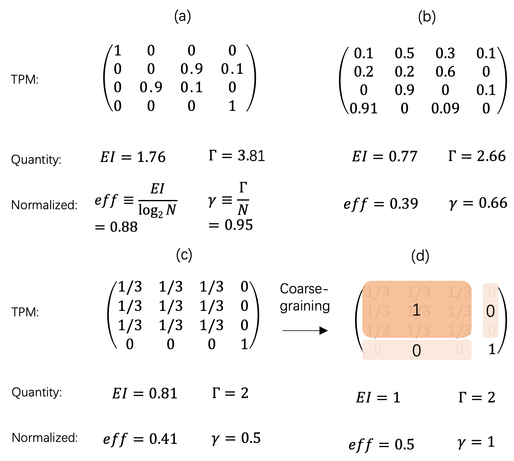
Figure 1: Examples of transitional probability matrices (TPMs) used in different Markov chains, along with measures of effective information (EI and normalized one $eff$) for causality, and the measure of $\Gamma$ (and normalized one $\gamma$) for reversibility of dynamics.

As the four cases of TPMs shown in Figure 1, the $EI$ values and their normalized forms $eff\equiv EI/\log_{2}N$ are also demonstrated below. As the TPM is closed to a permutation matrix, $EI$ is larger. Actually, $EI$ can reach its maximum when $P$ is reversible (that is $P$ is a permutation matrix according to Theorem 2 and 3 presented in Appendix E.1. In this case, $\bar{P}=\mathbbm{1}/N$, and $EI=\log_{2}N$). The example in Figure 1(d) is the coarse-grained TPM of example in Figure 1(c) by collapsing the first three rows and columns into one macro-state. $EI=1$(or $eff=0.5$) in (d) is clearly larger than $EI=0.81$(or $eff=0.41$) in (c), which manifests that the strength of cause-effect in macro-level (coarse-grained TPM in (d)) is larger than the micro-level (c), thus, causal emergence occurs.

Second, we will introduce a quantitative indicator to measure the reversibility of dynamics for a Markov chain.

Firstly, it is important to clarify that in this context, a dynamically reversible Markov chain refers to a chain where its $P$ is reversible, and its inverse $P^{-1}$ also serves as an effective TPM [16]. This definition differs from the commonly used term “time reversible” Markov chain [20], as dynamical reversibility necessitates the ability of $P$ to be reversibly applied to each individual state, whereas the latter focuses on the reversibility of state space distributions. Actually, we can prove that the former implies the latter (Theorem 4 in Appendix E).

However, in the case of a general TPM, it is not inherently reversible. Hence, an indicator that can quantify the degree to which a TPM deviates from being reversible is required.

Definition 1.

Suppose the transitional probability matrix (TPM) is $P$ for a markov chain $\chi$, and its singular values are $(\sigma_{1}\geq\sigma_{2}\geq\cdot\cdot\cdot\sigma_{N}\geq 0)$, then the measure of dynamical reversibility is:

$$\Gamma\equiv\sum_{i}^{N}\sigma_{i}.$$ (3)

In literateurs [21, 22, 23], $\Gamma$ is called nuclear norm or $p$-Schatten norm with $p=1$, and it is always treated as the continuous relaxation of the rank of matrix $P$.

The reason why $\Gamma$ can quantify the reversibility of $P$ is clear if we make an SVD decomposition on $P$:

$$P=U\cdot\Sigma\cdot V^{T},$$ (4)

where, $U$ and $V$ are two orthogonal and normalized matrices with dimension $N\times N$, and $\Sigma=diag(\sigma_{1},\sigma_{2},\cdot\cdot\cdot,\sigma_{N})$ is a diagonal matrix which contains all the ordered singular values. To be noticed that $U$ and $V^{T}$ are all reversible operators(matrices), therefore, the reversibility of $P$ is solely determined by $\Sigma$. If there are zero singular values in $\Sigma$, then $P$ in irreversible. If all the singular values are much larger than zero, $P$ is more reversible.

We actually can prove strictly that 1)$\Gamma$ achieves its maximal value $N$ when $P$ is reversible (Theorem 5 and Theorem 3, see Appendix E.2); and 2)If $P$ is closed to be reversible (a permutation matrix), then $\Gamma$ also approaches its maximal value $N$ in the same time (Theorem 7, see Appendix E.2).

In the four examples of Figure 1, $\Gamma$ varies from 2 to 3.81, and it is dependent on the system size $N$. To compare the reversibility measures across different sizes, we normalize $\Gamma$ by dividing $N$ to obtain $\gamma=\Gamma/N\in[0,1]$, it varies from 0.5(case c) to 1(case d) in Figure 1. It is clear that $\gamma$ is larger if the TPM is closed to a permutation matrix(reversible matrix).

Next, we will compare $\Gamma$ and $EI$ on similarities and differences.

First, $\Gamma$ and $EI$ can reach their maximal values $N$ and $\log(N)$, respectively, when $P$ is reversible (permutation matrix) according to Theorem 2 and Theorem 5 (See Appendix E.2). They also achieve their minimal values ($EI_{min}=0$ and $\Gamma_{min}=1$) according to Theorem 1 and Theorem 6, see Appendix E.1) when $P_{i}=\mathbbm{1}/N,\forall i\in[1,N]$. However, we can prove that $\mathbbm{1}/N$ is not the unique minimum solution of $EI$, any TPM with $P_{i}=P_{j}$ for any $i,j\in[1,N]$ can make $EI=0$. Therefore, $EI$ is not a convex function but $\Gamma$ is (see Theorem 6 and Corollary 1, Appendix E.2), as a result, the latter is more suitable for optimization.

Secondly, both $EI$ and $\Gamma$ are correlated with the auto-correlation matrix $P\cdot P^{T}$. As expressed in Equation 1, $EI$ actually is the “de-similarity” between each $P_{i},\forall i\in[1,N]$ and their average $\bar{P}$, measured by KL-divergence. While, any entry in $P\cdot P^{T}$ is the similarity between $P_{i}$ and $P_{j},\forall i,j\in[1,N]$ but measured by inner product. On the other side, all squared singular values of $P$ are the eigenvalues of $P\cdot P^{T}$, and $\Gamma$ is the trace of $\sqrt{P\cdot P^{T}}$ and it also decreases when all $P_{i}$s are similar(see Theorem 5 in Appendix E.1).

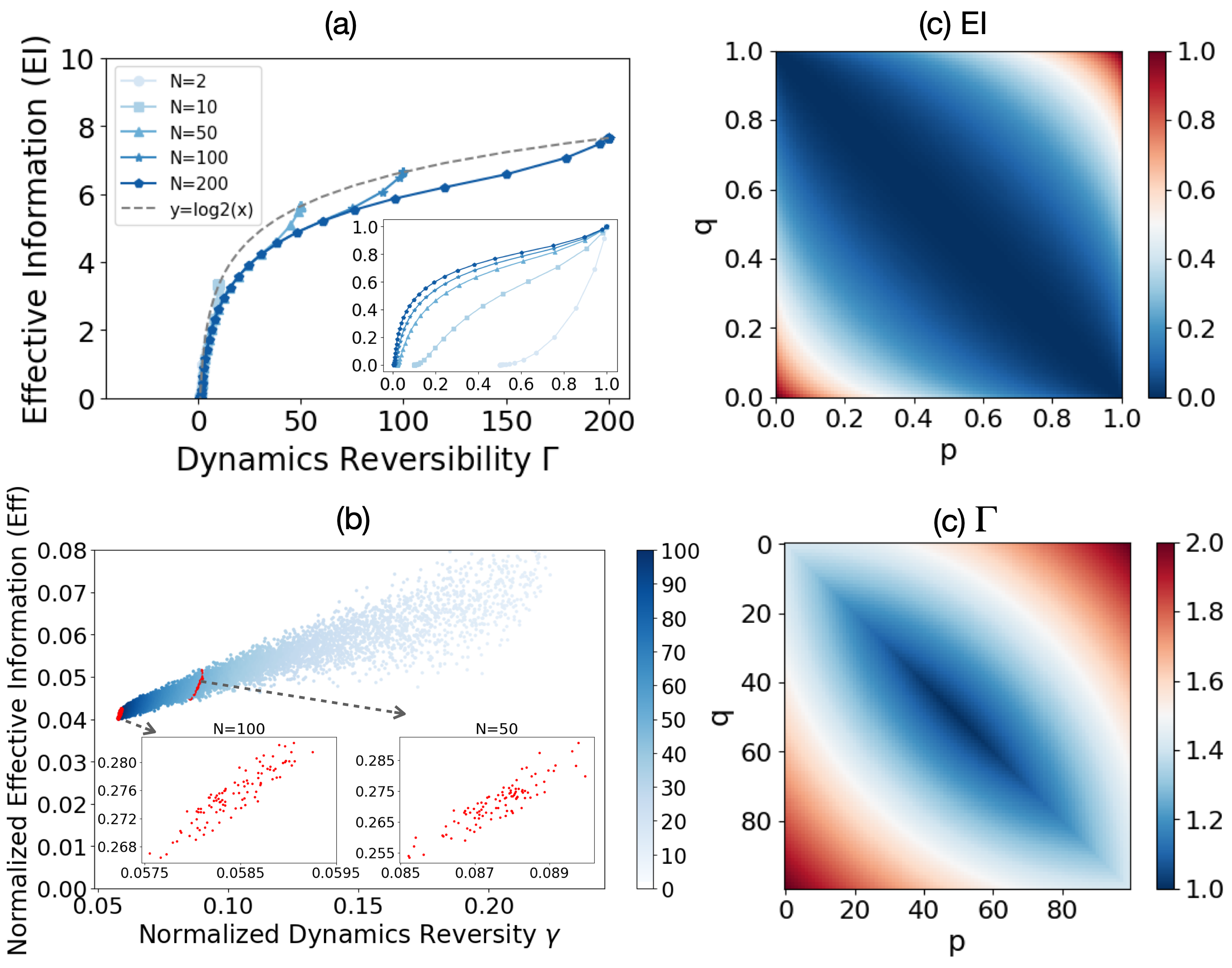
Figure 2: Comparison between $EI$ and $\Gamma$ for various randomly generated TPMs. (a) shows the approximately asymptotic relationship $EI\sim\Gamma$ for randomly generated TPMs which are perturbations of permutation matrices, the inset shows the normalized one. Each curve is obtained by tune up the magnitude of perturbation on a randomly generated permutation matrix with different sizes. (b) demonstrates the same relationship between normalized $Eff$ and $\gamma$ for the TPMs which are the combination of $N$ randomly sampled normalized row vectors for various sizes ($N\in[2,100]$) with different colors. On each size, 100 such random matrices are sampled to get the scatter points with a same color. The inset shows two exampled scatter point plots for particular sizes $N=50,100$. (c) and (d) shows the density plots of $EI$(c) and $\Gamma$(d) with different parameters $p$ and $q$ computed for a parameterized simplest TPM: $P=\begin{pmatrix}p&1-p\\ 1-q&q\end{pmatrix}$ with size $2\times 2$

We further compare $\Gamma$ and $EI$ on a variety of TPMs generated by a random perturbation on a randomly selected permutation matrix with size $N$ or composed by random normalized row vectors (the details are in Appendix A). As shown in Figure 2(a) and (b), a positive correlation is observed on all these examples, and an approximately asymptotic relationship is conjectured for large $N\gg 1$:

$$EI\sim\log\Gamma.$$ (5)

This relation is obviously observed in Figure 2(a), but degenerates to a nearly linear relation in Figure 2(b) since limited value region of $\Gamma$ is covered. However, the logarithm relation of Equation 5 can also be observed in another set experiments by controlling the degeneracy of the TPM (see Appendix A.3).

We also obtain the analytic solution for $EI$ and $\Gamma$ on the simplest parameterized TPM with size $N=2$(see Appendix B), and we show the landscape how $EI$ and $\Gamma$ are dependent on the parameters $p$ and $q$. It is clear that both $EI$ and $\Gamma$ obtain their maximum values on the anti-diagonal regions ($p=q=0$ or $p=q=1$, in this case, $P$ is a permutation matrix). The differences between Figure 2(c) and (d) are apparent: 1)$\Gamma$ has a peak value when $p\approx 1-q$ but $EI$ has not; 2) a broader region with $EI\approx 0$ is observed, while the region with $\Gamma\approx 1$ is much smaller; 3)an asymptotic transition from 0 to maximal $N=2$ is observed for $\Gamma$, but not for $EI$.

Therefore, we conclude $EI$ and $\Gamma$ are highly correlated on various TPMs. This implies we may use $\Gamma$ to replace $EI$ to build a new theory of causal emergence.
We have witness the power of singular values to characterize the property of the Markov dynamics in previous sections, therefore, we will build such a theory based on singular values. First, we will give two definitions for causal emergence.

Definition 2.

For a given markov chain $\chi$ with TPM $P$, if $r\equiv rank(P)<N$ then clear causal emergence occurs in this system. And the degree of causal emergence is

$$\Delta\Gamma=\Gamma\cdot(1/r-1/N).$$ (6)

This definition is independent of any coarse-graining method or external parameters. As a result, it represents an intrinsic and objective property of Markov dynamics.

Definition 3.

For a given markov chain $\chi$ with TPM $P$, suppose its singular values are $\sigma_{1}\geq\sigma_{2}\geq\cdot\cdot\cdot\geq\sigma_{N}$. For a given small real value $\epsilon$, if there is an integer $r\in[1,N)$, such that $\sigma_{r+1}<\epsilon$, then there is vague causal emergence with the level of vagueness $\epsilon$ occured in the system. And the degree of causal emergence is:

$$\Delta\Gamma(\epsilon)=\frac{\sum_{i=1}^{r}\sigma_{i}}{r}-\frac{\sum_{i=1}^{N}\sigma_{i}}{N}.$$ (7)

This definition applies when there is no distinct cutoff in the singular value spectrum, necessitating the manual selection of a threshold $\epsilon$.

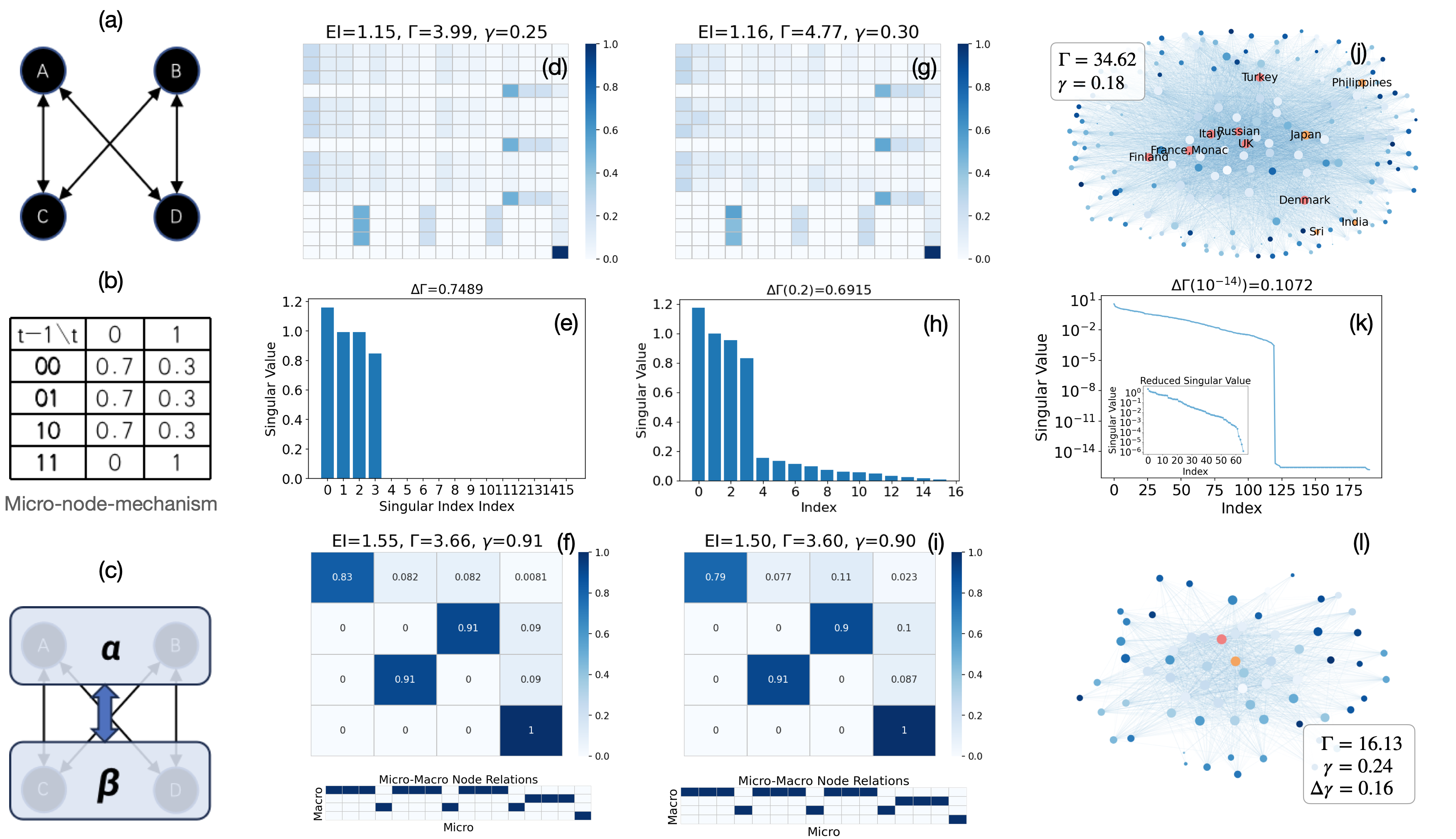
Figure 3: Examples of clear and vague causal emergence and their coarse-grained models based on SVD method. (a) The original stochastic boolean network model, each node can only interact with its network neighbors; (b) Node dynamics in (a). Each row corresponds to the states combination of one node’s all neighbors in previous time step, and each column is the probability that to take 0 or 1 of the node at current time step. (c) The coarse-grained boolean network of (a) which is extracted from the TPMs of (f) and (i). (d) The corresponding TPM of (a) and (b). (e) The singular value spectrum for (d). (g) A perturbed TPM from (d). (h) The singular value spectrum for (g). (f) and (i) are the reduced TPMs and the projection matrices (below) after the applications of our coarse-graining method on the original TPMs in (d) and (g), respectively. (j) is the original network of global trade flows at year 2000(with 190 countries as nodes, and 7,074 directed weighted edges representing the total trade flows between two countries of all products at that year). The TPM is obtained by normalizing each node’s export flow. (l) is the reduced network of (j) by utilizing our coarse-graining method twice (with 66 country clusters as nodes, and 1,382 coarse-grained trade flows as edges). The clusters of countries represented by Japan and Russian are highlighted in different colors in (j) and (l).

Two examples of TPMs for clear emergence and vague emergence are shown in Figure 3(a-i), respectively. The TPM in Figure 3(d) is derived from the boolean network and its node-mechanism in Figure 3(a) and (b) directly. Their singular value spectra are shown in Figure 3(e). There are only 4 non-zero singular values (Figure 3(e)) for the first example in (d), therefore, clear causal emergence occurs, and the degree of causal emergence is $\Delta\Gamma=0.75$.

Vague causal emergence can be shown on the TPM in Figure 3(g), which is derived from (d) by adding random Gaussian noise with strength ($\sigma=0.03$) on the TPM in (d). As a result, the singular spectrum is obtained as shown in Figure 3(h). We select $\epsilon=0.2$ as the threshold such that only 4 large singular values are left. The degree of causal emergence is $\Delta\Gamma(0.2)=0.69$.

Therefore, the occurrences of both clear and vague causal emergence, as well as the extent of such emergence, can be objectively quantified without dependence on any specific coarse-graining method.
Finally, our theory can also provide a concise coarse-graining method based on the singular value decomposition of $P$ to obtain a macro-level reduced TPM. The basic idea is to project the row vectors $P_{i},\forall i\in[1,N]$ in $P$ onto the sub-spaces spanned by the eigenvectors of $P\cdot P^{T}$ such that the major information of $P$ is conserved, as well as $\Gamma$ is kept unchanged. The coarse-graining method contains five steps: 1). SVD decomposition for the TPM according to Equation 4; 2) selecting an $\epsilon$ as the threshold to cut off the singular value spectrum, and to obtain $r(\epsilon)$ as the number of retained states; 3)dimensionality reduction for all $P_{i}$ in $P$ by calculating $P\cdot V_{N\times r}$, where only the first $r$ eigenvectors are retained; 4)clustering all row vectos in $P\cdot V_{N\times r}$ into $r$ groups to obtain a projection matrix $\Phi$; and 5) obtain a new TPM by using $\Phi$ and $P$ such that the total stationary flux is kept unchanged. If there is clear cut off of the singular value spectrum of the reduced network, then repeat the steps from 1) to 5). The detailed information about this method and why it does work can be referred in Appendix C.

We test our method on the two examples shown in Figure 3(d) and (g), and the coarse TPMs are shown in (f) and (i). The macro-level boolean network model(3 (c)) can be read out from the TPMs and the projection matrix $\Phi$. To be noticed, $\Gamma$s in the coarse TPMs are almost identical to the original ones, which means our method is $\Gamma$ conservative. We further test the examples of causal emergence in the references [5, 6], and almost identical coarse TPMs can be obtained.

Finally, to illustrate one of the potential applications, we employ our method on the world trade network in 2000(Figure 3(j)) to obtain a coarse-grained network, as depicted in Figure 3(l). In which, fewer than half the original nodes and only about one-seventh of the edges are retained, while the measure $\Gamma$ is halved. Interestingly, the degree of causal emergence, as assessed by the normalized measure $\gamma$, actually rises. Consequently, a smaller and more tightly connected core network is identified, which facilitates the major trade flows.

In summary, we have discovered that the nuclear norm, which is the sum of all singular values of a TPM, can be utilized to quantify the reversibility of the Markov dynamics. Both theoretical findings and empirical experiments provide support for the existence of positive correlation, where the $EI$ is approximately and asymptotically proportional to the logarithm of the measure $\Gamma$. Building upon this measure, we have developed a new theory of causal emergence that provides a clearer definition, reflecting the intrinsic properties of the system and independent of any specific coarse-graining method. Additionally, through the SVD decomposition of a TPM, we have identified a more concise approach to coarse-grain the system.

Further, this work establishes a potential link between thermodynamics and causal emergence. The emergence of causation corresponds to the emergence of dynamical reversibility, which in turn implies a reduction in entropy. Therefore, the interest in emergent behaviors can be explained by the desire to achieve macro-dynamics with a lower rate of entropy production. However, this is contingent upon the entropy production during the process of coarse-graining. Hence, the balance between the rates of entropy productions in macro-dynamics and coarse-graining deserves further attention.

Nevertheless, there are limitations in this work. Firstly, all the aforementioned discussions have been centered around the state space, whereas an extension to the variable space would be more practical. However, it should be noted that the size of the state space grows exponentially with the number of variables, which poses a challenge. Secondly, while $\Gamma$ is a convex function that aids in optimization, it cannot be decomposed into determinism and degeneracy like $EI$ [5], thereby reducing its interpretability. As a result, further research is warranted to address these issues.

Appendix A Experiments on testing the correlation between $EI$ and $\Gamma$

In this section of the appendix, we will introduce the details of our experiments on the relationship between dynamical reversibility $\Gamma$ and $EI$ on various generated TPMs. The generative model of TPMs have three classes: perturbation on permutation matrix, random normalized, and perturbation on controlled degenerative TPMs.

A.1 Perturbation on Permutation Matrix

In this series experiments, we will find out what the relationships between $\Gamma$ and $EI$ are on a variety of TPMs with different deviations from the reversible TPMs (permutation matrix) and different sizes.

For given size $N$, The TPM is generated by three steps: 1). Randomly sample a permutation matrix with dimension $N\times N$; 2). For each row vector $P_{i}$ in $P$, and suppose the position of the sole 1 element is $j_{i}$, fill out all entries of $P_{i}$ with the probabilities of a Gaussion distribution center at $j_{i}$, that is, $P^{\prime}_{i,j}=\frac{1}{\sqrt{2\pi}\sigma}\exp{-\frac{(j-j_{i})^{2}}{\sigma^{2}}}$, where, $j_{i}$ is the position where the sole 1 element locates in $P_{i}$, and $\sigma$ is a free parameter; 3). Normalize this new row vector $P^{\prime}_{i}$ by dividing $\sum_{j=1}^{N}P^{\prime}_{ij}=1$, such that the modified matrix $P^{\prime}$ is also a TPM.

In this model, the unique parameter $\sigma$ can control the degree of deviations from the original TPM. When $\sigma=0$, we recover the original TPM. And when $\sigma$ increases to very large value, then the row vectors converge to the vector $\mathbbm{1}/N$. Figure S1 shows the TPMs before and after the update on $\sigma=10$, where the colors represent the probabilities.

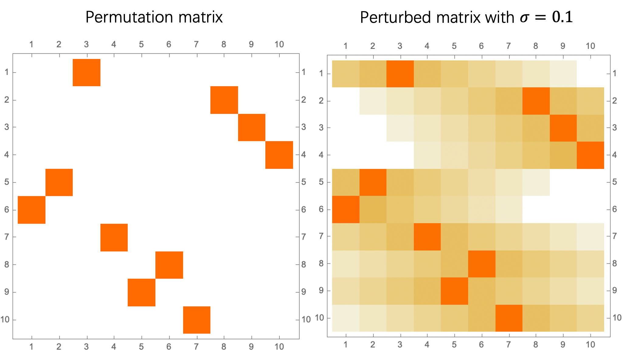
Figure S1: The original TPM and the perturbed one.

A.2 Random Normalization

In this model, only two step can generate a TPM: 1). Sample a row random vector, 2) normalize this row vector such that the generated matrix is a TPM.

A.3 Perturbation on Controlled Degeneracy

The third model is very similar to the first one, however, the original matrix is not a permutation matrix, but a degenerated permutation matrix. Here, a TPM is degenerative means that there are some row vectors are identical, and the number of identical row vectors is denoted as $\alpha$ which is the controlled variable. By tuning $\alpha$, we can control the degeneracy [5] of the $TPM$ as Figure S2 shows.

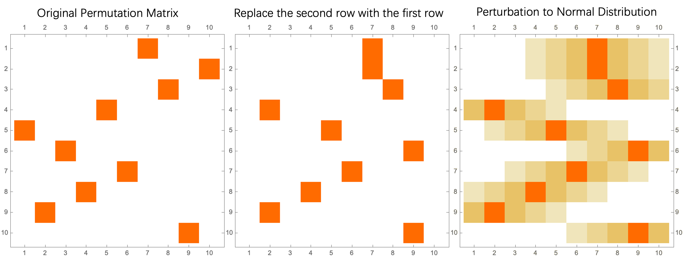
Figure S2: The original TPM, the replaced one to by controlling $\alpha=2$, and the perturbed TPM of the replaced one. Different colors represent different values of probability.

The experimental results are as follows. First, we will justify if degeneracy of the TPM can be controlled by $\alpha$. We work with a $100\times 100$ matrix, progressively adjusting $\alpha$ from 0 to 99, corresponding to the process of increasing degeneracy. We also introducing disturbance noise as another control parameter, here we test $\sigma$ from $10^{-3}$ to $10^{3}$. Figure. S3(a) shows the degeneracy of different disturbance change as $\alpha$ . Figure S3(b) shows EI versus $\Gamma$ for different degeneracy.

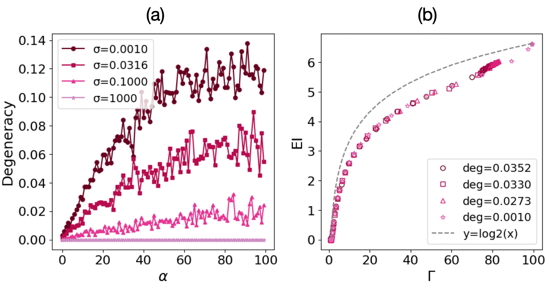
Figure S3: (a). Degeneracy of different disturbance change as $\alpha$. Here, we choose $\sigma=0.001,1000$, 1/2 and 1/3 quantiles under logarithmic division, that is $\sigma=0.0316,0.1$ to display. (b). EI versus $\Gamma$ for different degeneracy. Each point here is the average result of a different certainty under different disturbance noise $\sigma$.

Appendix B Analytic solutions on the parameterized 2*2 TPM

We compare $EI$ and $\Gamma$ on a simplest example, the TPM is as:

$$P=\begin{pmatrix}p&1-p\\ 1-q&q\end{pmatrix},$$ (1)

where $p$ and $q$ are all free parameters in the range of $[0,1]$. With this TPM, we can explicitly write down the expression for $EI$:

$$EI= \frac{1}{2}\left[p\log_{2}\frac{2p}{1+p-q}+(1-p)\log_{2}\frac{2(1-p)}{1-p+q}\right.$$ (2)

$$+\left.(1-q)\log_{2}\frac{2(1-q)}{1+p-q}+q\log_{2}\frac{2q}{1-p+q}\right],$$

and $\Gamma$:

$$\Gamma=\sqrt{p^{2}+(1-p)^{2}+(1-q)^{2}+q^{2}+2|1-q-p|}.$$ (3)

According these two expressions, we plot the landscapes in Figure 2(c) and (d).

Appendix C The coarse graining method based on SVD decomposition

We will first give the detailed introduction of the coarse-graining method based on SVD, and then we give an explanation why this simple method can work in practice.

C.1 The method

Intuitively, the basic idea of our method is to treat all row vectors $P_{i}$ in $P$ as data vectors with dimensionality of $N$, then we first take $PCA$ dimensionality reduction for these row vectors, second to cluster them into $r$ clusters where $r$ is selected according to the threshold $\epsilon$ for singular value spectrum. With the clusters, we can reduce the original TPM according to the principle that all the stationary flows are conservative.

Concretely, the coarse-graining method contains five steps:

1) We first make SVD decomposition for $P$ (suppose $P$ is irreducible and recurrent such that stationary distribution exist):

$$P=U\cdot\Sigma\cdot V^{T},$$ (4)

where, $U$ and $V$ are two orthogonal and normalized matrices with dimension $N\times N$, and $\Sigma=diag(\sigma_{1},\sigma_{2},\cdot\cdot\cdot,\sigma_{N})$ is a diagonal matrix which contains all the ordered singular values.

2) Selecting a threshold $\epsilon$ and the corresponding $r$ if there is a clear cut off on the singular value spectrum;

3) Reducing the dimensionality of row vectors $P_{i}$ in $P$ from $N$ to $r$ by calculating the following Equation:

$$P^{\prime}\equiv P\cdot V_{N\times r},$$ (5)

where $V_{N\times r}=(V_{1}^{T},V_{2}^{T},\cdot\cdot\cdot,V_{r}^{T})$.

4) Clustering all row vectors in $P^{\prime}$ into $r$ groups by K-means algorithm to obtain a projection matrix $\Phi$, which is defined as:

$$\Phi_{ij}=\begin{cases}1&\mbox{if $P_{i}^{\prime}$ is in the $r$th group}\\ 0&\mbox{otherwise},\end{cases}$$ (6)

for $\forall i,j\in[1,N]$.

5) Obtain the reduced TPM according to $P$ and $\Phi$.

To illustrate how we can obtain the reduced TPM, we will first define a matrix called stationary flow matrix as follows:

$$F_{ij}\equiv\mu_{i}\cdot P_{ij},\forall i,j\in[1,N],$$ (7)

where $\mu$ is the stationary distribution of $P$ which satisfies $P\cdot\mu=\mu$. In the example of trade network in the main text, $F$ is actually proportional to the trade flow matrix of the whole network.

Secondly, we will derive the reduced flow matrix according to $\Phi$ and $F$:

$$F^{\prime}=\Phi^{T}\cdot F\cdot\Phi,$$ (8)

where, $F^{\prime}$ is the reduced stationary flow matrix. The trade flow network in Figure 3(l) is obtained by $F^{\prime}$ and multiplying the total trade volume of each country. Finally, the reduced TPM can be derived directly by the following formula:

$$P^{\prime}_{i}=F^{\prime}_{i}/\sum_{j=1}^{N}(F^{\prime}_{i})_{j},\forall i\in[1,N].$$ (9)

Finally, $P^{\prime}$ is the coarse-grained TPM.

If there is still apparently cut-off in the singular value spectrum of $P^{\prime}$, then repeat step 2) to 5). The reduced flow network in the example of trade network is obtained by running 1) to 5) twice.

C.2 Explanation

We will explain why this coarse-graining strategy outlined in the previous sub-section works here.

In the first step, the reason why we SVD decompose the matrix $P$ is that the singular values of $P$ actually are the squared roots of the eigenvalues of $P^{T}\cdot P$ because:

$$P^{T}\cdot P=(P\cdot P^{T})^{T}=(V\cdot\Sigma\cdot U^{T})\cdot(U\cdot\Sigma\cdot V^{T})=V\cdot\Sigma^{2}\cdot V^{T},$$ (10)

thus, we will try our best to utilize the corresponding eigenvectors in $V$ to reduce $P$, because they may contain more important information of $P$.

Actually, the eigenvectors with the largest eigenvalues are the major axes to explain the auto-correlation matrix $P^{T}\cdot P$. Therefore we can use PCA method to reduce the dimensionality of $P_{i},\forall i\in[1,N]$s, it is equivalent to projecting $P_{i}$ onto the subspace spanned by the $r$ first eigenvectors.

In the fourth step, we cluster all the row vectors $P_{i},\forall i\in[1,N]$ into $k<r$ groups according to the new feature vectors of $P_{i}$. Actually, according to the previous studies [24], these $r$ major eigenvectors can be treated as the centroids of the clusters obtained by K-means algorithm for the row vectors $P_{i},\forall i\in[1,N]$. Therefore, we cluster all row vectors in $P$ by K-means algorithm, and the row vectors in one group should aggregate around the corresponding eigenvectors.

The final step is to obtain the reduced TPM according to the clustering result or $\Phi$ in the previous step. This is a classic problem of lumping a Markov chain [25, 26]. There are many lumping methods, and we adopt the one in  [27].

The basic idea of this method is to keep the stationary distribution and the total stationary flux unchanged during lumping process because they can be understood as a conservative quantity such as trade volume. As a result, we derive the method mentioned in the previous sub-section.

Appendix D Applying our coarse-graining method on more examples

D.1 Examples of boolean networks in Hoel(2003)

To compare our method and EI maximization method, we apply our method to the examples of causal emergence in Hoel et al’s original papers [5] and [6]. All the examples show clear causal emergence. And almost identical reduced TPMs are obtained for all the examples.

In Figure S4, we present the results for the same example Hoel mentioned, which uses a directed Boolean network of 6 nodes. Our findings align perfectly with Hoel’s, proving that the equivalence of the two theoretic frameworks.

Figures S5 and S6 show additional examples from the SI, where our model predicts a higher macro EI compared to Hoel’s findings. The main difference lies in our approach: Hoel groups variables to form a new macro network and then calculates EI for the TPM. We, on the other hand, group states directly, which might result in a TPM that doesn’t fully represent the original Boolean network in terms of variables. Therefore, the extension of our method to variable-based coarse-graining method is deserve future studies.

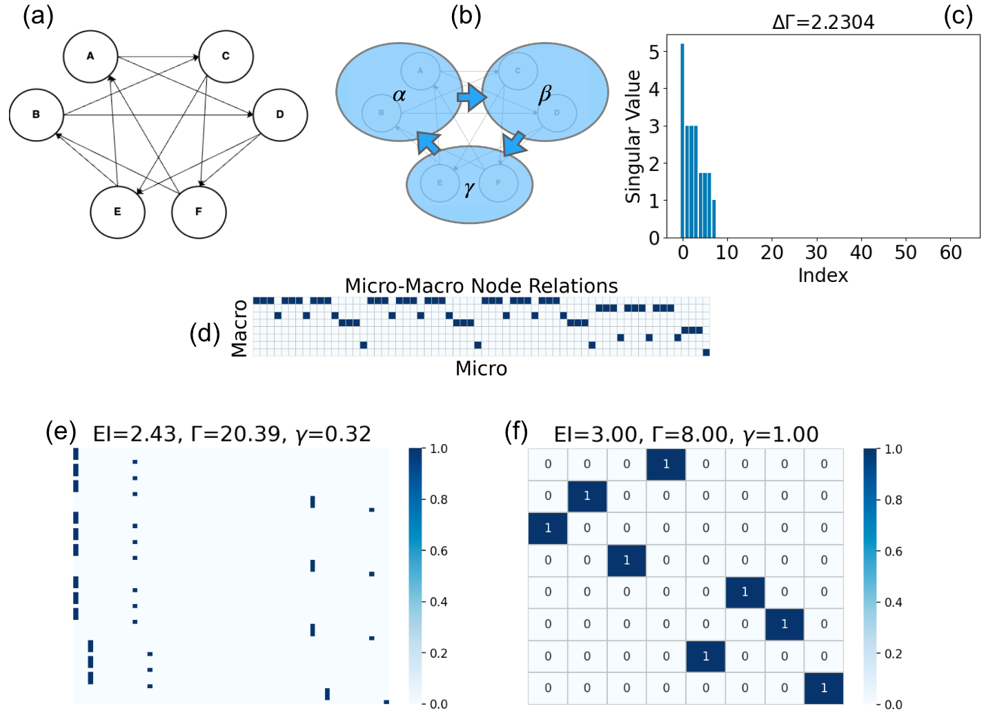
Figure S4: Directed boolean network with 6 nodes. (a) and (b) are micro and macro network respectively. (c) is the singular spectuam of micro TPM. (d) is projection matrix from our method. (e) and (f) are corresponding TPM of (a) and (b). The result is totally consistent with [5].

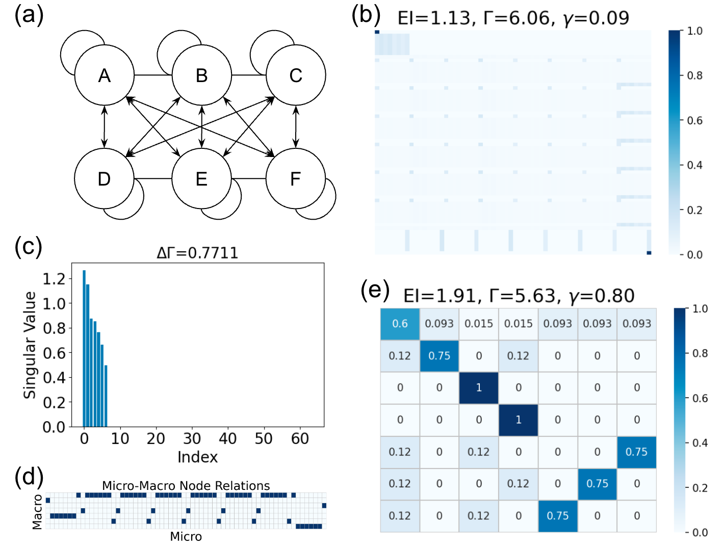
Figure S5: (a) is a full-connection boolean network with two different types of edges. (b)is TPM reproducted from for Fig.S2 of [5]. (c) is the singular spectuam of (b). (d) is projection matrix. (e)is coarse-grained TPM with our method. Here we get a larger macro EI than [5] (1.91 here and 1.84 in Hoel et al.’s work). It is because the macro TPM in [5] has 9 states, while our results only have 7. They treats {000111} and {111000} as two separate additional macro state as {02} and {20}, while ours treats them as {11}.

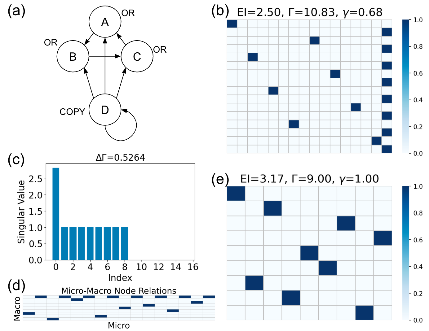
Figure S6: (a) is a directed booloean network. (b) is the TPM of (a). (c) is the singular spectuam of (b). (d) is projection matrix. (e) is course-grained TPM. We also get a larger macro EI than Hoel’s (3.17 here and 3.00 in [6]). It is because we have 9 macro states and [6] only has 8. We combined all the 8 micro states that transform to {11111111} as a seperate macro state, while [5] combines them into each of the other 8 groups.

D.2 Example of trade flow network in 2000

To show one of the potential applications of our coarse-graining method, we apply the method on international trade network. The dataset is downloaded from the NBER-United Nations trade data (http://cid.econ.ucdavis.edu/nberus.html), and it covers the details of world trade flow from 1962 to 2000, and SITC4 (4-digit Standard International Trade Classification,Revision 4) standard [23] is used to organize hundreds types of products in the dataset. We select the network at year 2000 and ignore the products and aggregate the trade flows for all products. The network contains 190 nodes(countries) and 7,074 edges(trade relations) with weights representing trade flows.

Suppose the trade flow matrix is $F$, where each entry $F_{ij}$ represents the trade flow from country $i$ to $j$, then the TPM is calculated as:

$$P_{ij}=F_{ij}/\sum_{k=1}^{N}F_{ik},\forall i,j\in[1,N].$$ (11)

We plot the spectrum of singular values of $P$ as shown in Figure S7.

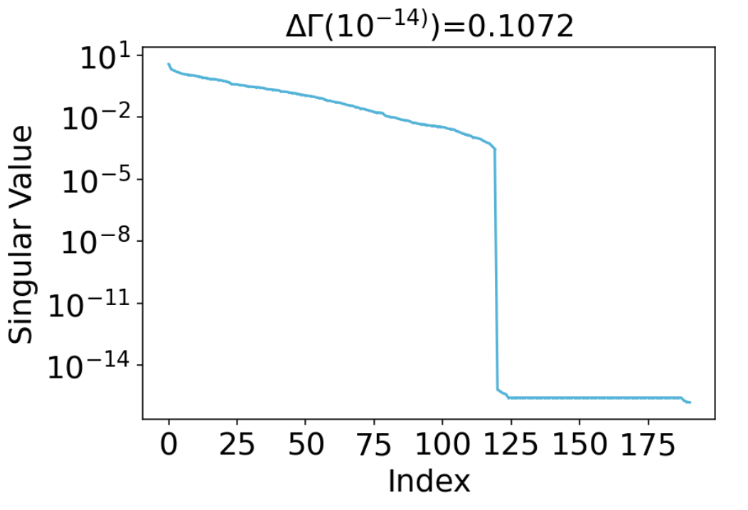
Figure S7: Spectrum of singular values for original network.

And there is an apparent cut off, thus we implement the coarse-graining method mentioned in section C on this network to obtain a reduced network. The threshold $\epsilon$ is set as $10^{-14}$, and the corresponding $r=120$.

Next, we further plot the singular value spectrum as shown in Figure S8(a).

And there still is an apparent cut off, thus we run the coarse-graining method on this reduced network. The threshold $\epsilon$ is set $10^{-8}$, and the corresponding number of retained nodes $r=66$ to obtain the final reduced network as shown in Figure 3(l), and the spectrum of this final network is as shown in Figure S8(b).

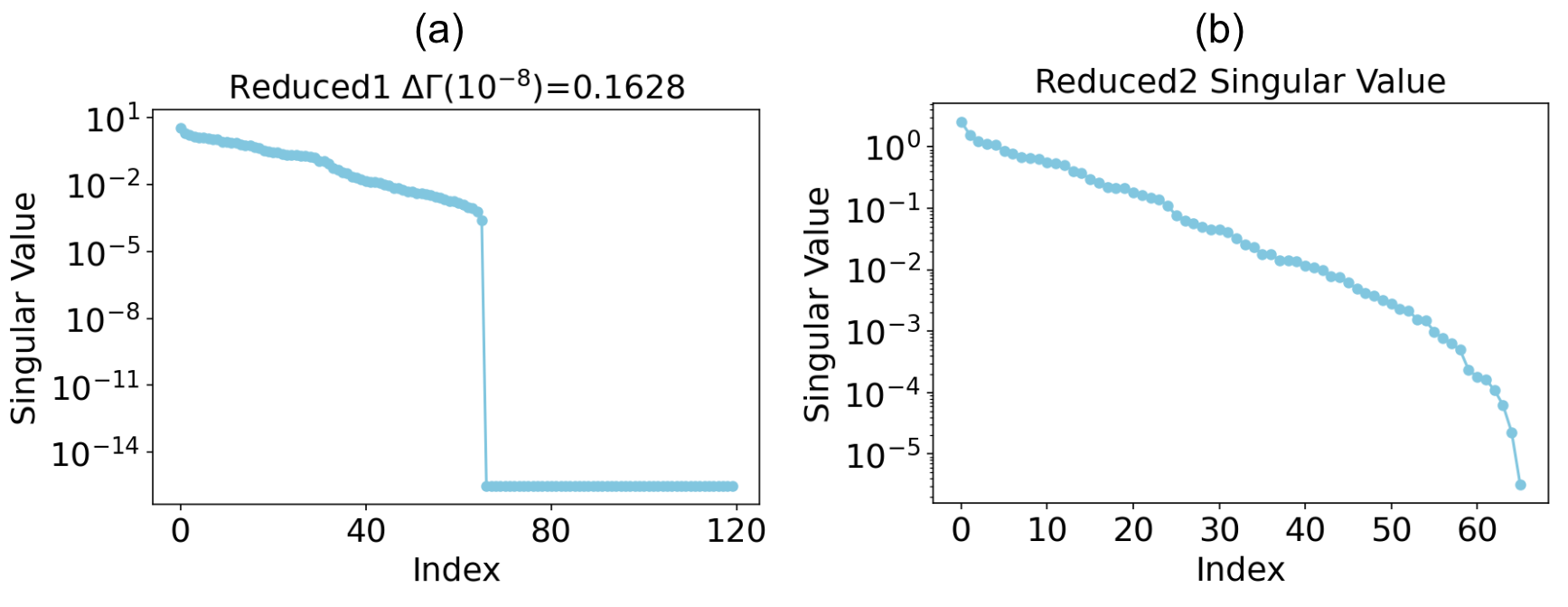
Figure S8: Spectrum of singular values for reduced networks. (a) and (b) are the results of the first and the second implementations of our coarse-graining method, respectively.

Appendix E Theorems and Proves

E.1 Theorems and proves for $EI$

We will layout the theorems about $EI$ and give the proves for them in this sub-section.

Theorem 1.

The $EI$ can reach its minimum at $0$ if and only if the row vectors of the probability transition matrix $P$ are identical.

Proof.

The $EI$ can be expressed as:

$$EI=\frac{1}{N}\sum_{i=1}^{N}D_{KL}(P_{i}||\bar{P})=\frac{1}{N}\sum_{i=1}^{N}\sum_{j=1}^{N}p_{ij}\log\frac{N\cdot p_{ij}}{\sum_{k=1}^{N}p_{kj}},$$ (12)

where, $P_{i}$ is the $i$th row vector in $P$, and $\log$ is the logarithm function with base $2$. By taking derivative, and using the normalization condition of probability distribution $\sum_{j=1}^{N}p_{ij}=1$ for $1\leq i\leq N$, we obtain that:

$$\frac{\partial EI}{\partial p_{ij}}=\log\left(\frac{p_{ij}}{p_{iN}}\right)-\log\left(\frac{\bar{p}_{\cdot j}}{\bar{p}_{\cdot N}}\right)$$ (13)

for $1\leq i\leq N$ and $1\leq j\leq N-1$, where $\bar{p}_{\cdot j}=\frac{1}{N}\sum_{k=1}^{N}p_{kj}$ for $1\leq j\leq N$. Therefore, Equation 13 is equal to 0 if and only if:

$$p_{ij}=p^{*}_{ij}=\bar{p}_{\cdot j}=\frac{1}{N}\sum_{k=1}^{N}p_{kj}$$ (14)

for any $1\leq i,j\leq N$. That is to say, all the row vectors are identical: $P_{i}=P_{j}=\bar{P}$ for any $1\leq i,j\leq N$. And the corresponding value of $EI$ is:

$$EI_{min}=0.$$ (15)

∎

Therefore, $EI$ can reach its minimum value $0$ when all the row vectors are identical. For the special matrix $P=\frac{1}{N}\cdot\mathbbm{1}$, $EI$ also equals 0, however, it is not the unique minimum point. Actually, all the matrix with identical normalized probability vector can make $EI=0$.

By further taking the second order derivative of $EI$, we can prove that $EI$ is not a convex function.

Corollary 1.

The second order derivative of $EI$ with respect to the distribution $p_{st}$ with $1\leq s\leq N$ and $1\leq t\leq N-1$ is:

$$\frac{\partial^{2}EI}{\partial p_{ij}\partial p_{st}}=\frac{1}{N}\cdot\left(\frac{\delta_{i,s}\delta_{j,t}}{p_{ij}}+\frac{\delta_{i,s}}{p_{iN}}-\frac{\delta_{j,t}}{N\cdot\bar{p}_{\cdot j}}-\frac{1}{N\cdot\bar{p}_{\cdot N}}\right),$$ (16)

and the $EI(\{p_{ij}\})$ is not a convex function.

Proof.

By further taking the derivative of Equation 13 with respect to the distribution $p_{st}$ with $1\leq s\leq N$ and $1\leq t\leq N-1$, we obtain Equation 16.

When $i=s$ and $j=t$, the second order derivative of $EI$ is:

$$\frac{\partial^{2}EI}{\partial p_{ij}^{2}} =\frac{1}{p_{ij}}+\frac{1}{p_{iN}}-\frac{1}{N\cdot\bar{p}_{\cdot j}}-\frac{1}{N\cdot\bar{p}_{\cdot N}}$$ (17)

$$=\frac{\sum_{k=1}^{N-1}p_{kj}-p_{ij}}{p_{ij}\cdot\bar{p}_{\cdot j}}+\frac{\sum_{k=1}^{N-1}p_{kN}-p_{iN}}{p_{iN}\cdot\bar{p}_{\cdot N}}$$

$$=\frac{\sum_{k\neq i}p_{kj}}{p_{ij}\cdot\bar{p}_{\cdot j}}+\frac{\sum_{k\neq i}p_{kN}}{p_{iN}\cdot\bar{p}_{\cdot N}}\geq 0,$$

but when $i\neq s$,

$$\frac{\partial^{2}EI}{\partial p_{ij}\partial p_{st}}=-\frac{\delta_{j,t}}{N\cdot\bar{p}_{\cdot j}}-\frac{1}{N\cdot\bar{p}_{\cdot N}}\leq 0$$ (18)

holds no matter if $j=t$ or not. Therefore, the Hessian matrix is not positive-definite, $EI$ is not a convex function. ∎

We will further discuss the condition and the properties of the maximum point of $EI$.

Theorem 2.

The effective information measure can reach its maximum $\log N$ if and only if $P$ is a permutation matrix.

Proof.

By noticing that

$$\sum_{i=1}^{N}\sum_{j=1}^{N}p_{ij}\log\bar{p}_{\cdot j} =\sum_{j=1}^{N}\left(\sum_{i=1}^{N}p_{ij}\right)\log\bar{p}_{\cdot j}$$ (19)

$$=\sum_{j=1}^{N}\bar{p}_{\cdot j}\log\bar{p}_{\cdot j}=-H(\bar{P}),$$

where $H(\bar{P})$ is the Shannon entropy of the average distribution $\bar{P}\equiv\sum_{i=1}P_{i}/N$. Thus, the $EI$ can also be separated as:

$$EI =\frac{1}{N}\sum_{i=1}^{N}\sum_{j=1}^{N}p_{ij}\log p_{ij}-\frac{1}{N}\sum_{i=1}^{N}\sum_{j=1}^{N}p_{ij}\log\bar{p}_{\cdot j}$$ (20)

$$=\frac{1}{N}\sum_{i=1}^{N}\left(-H(P_{i})\right)+H(\bar{P}).$$

Where $H(P_{i})=-\sum_{j=1}^{N}p_{ij}\log p_{ij}$ is the Shannon entropy of the distribution $P_{i}$. Furthermore, we have:

$$-H(P_{i})\leq 0,$$ (21)

the equality holds when $P_{i}$ is a one hot vector, and we also have:

$$H(\bar{P})\geq\log N,$$ (22)

and the equality holds when $\bar{P}=\frac{1}{N}\cdot\mathbbm{1}$. By combining these two inequality together, we can obtain:

$$EI\leq 0+\log N=\log N.$$ (23)

The condition that make the equality in Equation 21 and the equality in Equation 22 hold simantanously is that all row vectors in $P$ are one-hot vectors, and they are all different such that

$$\frac{1}{N}\sum_{i}P_{i}=\bar{P}=\frac{1}{N}\cdot\mathbbm{1}.$$ (24)

Therefore, we reach the statement claimed by this theorem that $P$ must be a permutation matrix.

∎

E.2 Theorems and proves for dynamical reversibility and $\Gamma$

E.2.1 Dynamical Reversibility and Time Reversibility

Theorem 3.

For a given markov chain $\chi$ and the corresponding TPM $P$, if $P$ simoutanously satisfy: 1. $P$ is reversible, that is, there is a matrix $P^{-1}$, such that $P\cdot P^{-1}=I$; and 2. $P^{-1}$ is also a TPM of another markov chain $\chi^{-1}$, then $P$ must be a permutation matrix.

Proof.

Because $P$ is reversible, therefore,

$$P=U\cdot diag(\lambda_{1},\lambda_{2},\cdot\cdot\cdot,\lambda_{N})\cdot U^{-1},$$ (25)

where, $\lambda_{1},\lambda_{2},\cdot\cdot\cdot,\lambda_{N}$ are the eigenvalues of $P$, and their modulus are less than or equal to 1:

$$|\lambda_{i}|\leq 1,\forall i\in[1,N],$$ (26)

these inequality holds because $P$ is a TPM of a Markov chain according to [28].

Thus, the inverse of $P$ can be expressed by:

$$P^{-1}=U\cdot diag(\lambda_{1}^{-1},\lambda_{2}^{-1},\cdot\cdot\cdot,\lambda_{N}^{-1})\cdot U^{-1},$$ (27)

and:

$$|\lambda_{i}|^{-1}\geq 1,\forall i\in[1,N],$$ (28)

However, this conflicts with the conclusion that the modulus of all the eigenvalues of a TPM must be less or equals to 1 if the inequality holds strictly. Thus, we have:

$$|\lambda_{1}|=|\lambda_{2}|=\cdot\cdot\cdot=|\lambda_{N}|=1.$$ (29)

Therefore, the eigenvalues are the complex solutions for the equation of $x^{N}=1$, thus $P$ is a permutation matrix. ∎

Next, we will prove dynamical reversibility implies time reversibility for Markov chains.

Theorem 4.

For a recurrent discrete Markov chain $\chi$, suppose its TPM is $P$ on the space of states $\mathcal{S}$ and its stationary distribution is $\mu$, if $P$ is dynamically reversible, then $\chi$ also satisfies time reversibility.

Proof.

Suppose $\chi$’s time reversed Markov chain is $\chi^{\prime}$, and its TPM $Q_{ij}\equiv P(X_{t}=s_{i}|X_{t+1}=s_{j})$, where $s_{i}$ and $s_{j}\in\mathcal{S}$ are the states at time steps $t$ and $t+1$, respectively. Then $P,Q,\mu$ should satisfy the detailed balance condition:

$$P(X_{t+1},X_{t})=P(X_{t},X_{t+1}),$$ (30)

By using Bayesian formulation,

$$P(X_{t},X_{t+1})=P(X_{t+1}|X_{t})P(X_{t})=P(X_{t+1})P(X_{t}|X_{t+1}),$$ (31)

and let $t\rightarrow\infty$ such that $P(X_{t})=P(X_{t+1})=\mu$, Equation 31 can be written as:

$$Q_{ij}\cdot\mu_{i}=P_{ji}\cdot\mu_{j}$$ (32)

If $\chi$ is time reversible, then $Q=P$, therefore:

$$P_{ij}\cdot{\mu_{i}}=P_{ji}\cdot\mu_{j}.$$ (33)

Equation 33 is the sufficient and necessary condition for $\chi$ being time reversible.

If $P$ is dynamically reversible, then $P$ is a permutation matrix, and satisfies $P=P^{-1}=P^{T}$, then the corresponding stationary distribution must be $\mathbbm{1}/N$ such that any permutation on elements in $\mathbbm{1}/N$ is the same vector. Therefore, by taking all these special values into Equation 33, we have

$$left=P_{ij}\cdot\frac{1}{N}=P_{ji}\cdot\frac{1}{N}=right.$$ (34)

Therefore, the dynamical reversibility of $\chi$ implies its time reversibility. But its reverse is not, apparently.

∎

E.2.2 The Measure of Dynamical Reversibility $\Gamma$

We will present the theorems and the proves about the measure of dynamical reversibility $\Gamma$ in this sub-section. Before the theorems are presented, we will prove the lemma related with the theorem that will be used in the following parts.

Lemma 1.

For a TPM $P=(P_{1},P_{2},\cdot\cdot\cdot,P_{N})^{T}$, where $P_{i}$ is the $i$-th row vector, then:

$$P_{i}\cdot P_{j}\leq 1,\forall i,j\in[1,N]$$ (35)

Proof.

Because $P_{i}$ is a probability distribution, therefore, it should satisfy normalization condition which can be expressed as:

$$|P_{i}|=\sum_{j=1}^{N}p_{ij}=1,$$ (36)

where, $|\cdot|$ is 1-norm for vector, which is defined as the summation of the absolute values of all elements. Thus:

$$P_{i}\cdot P_{j}=|P_{i}\cdot P_{j}|_{1}\leq|P_{i}|_{1}\cdot|P_{j}|_{1}=1.$$ (37)

∎

Lemma 2.

For a given TPM $P$, suppose its singular values are $(\sigma_{1},\sigma_{2},\cdot\cdot\cdot,\sigma_{N})$, we have:

$$\sum_{i=1}^{N}\sigma_{i}^{2}=\sum_{i=1}^{N}P_{i}^{2}\leq N$$ (38)

Proof.

Because $\sigma_{i}^{2},\forall i\in[1,N]$ are the eigenvalues of $P\cdot P^{T}$, thus, $P$ can be written:

$$P\cdot P^{T}=U\Sigma^{2}U^{T},$$ (39)

where $U$ is a orthonormal matrix with size $N$, $\Sigma^{2}=diag(\sigma_{1}^{2},\sigma_{2}^{2},\cdot\cdot\cdot,\sigma_{N}^{2})$. Thus,

$$\sum_{i=1}^{N}\sigma_{i}^{2} =\operatorname{Tr}{\Sigma^{2}}=\operatorname{Tr}{(U\Sigma^{2}U^{T})}=\operatorname{Tr}{\left(P\cdot P^{T}\right)}$$ (40)

$$=\sum_{i=1}^{N}P_{i}^{2}\leq N.$$

The last inequality holds because of Lemma 1. And the equality hold if and only if:

$$P_{i}\cdot P_{i}=1,\forall i\in[1,N]$$ (41)

∎

Lemma 3.

For a TPM $P$, we can write it in the following way:

$$P=(P_{1},P_{2},\cdot\cdot\cdot,P_{N})^{T},$$ (42)

where $P_{i}$ is the $i$-th row vector. And suppose $P$’s singular values are $\sigma_{1}\geq\sigma_{2}\geq\cdot\cdot\cdot\geq\sigma_{N}$. Thus, if

$$P_{i}\cdot P_{i}=1,\forall i\in[1,N],$$ (43)

then the singular values of $P$ satisfy:

$$\sigma_{1}\geq\sigma_{2}\geq\cdot\cdot\cdot\geq\sigma_{r}\geq 1$$ (44)

and

$$\sigma_{r+1}=\sigma_{r+2}=\cdot\cdot\cdot=\sigma_{N}=0,$$ (45)

where $r$ is the rank of the matrix $P$.

Proof.

If $P_{i}\cdot P_{i}=1$, then $\sum_{j}p_{ij}^{2}=1$, that means $P_{i}$ is a unit vector with modulus 1. While, $|P_{i}|_{1}=\sum_{j=1}^{N}p_{ij}=1$ for all $i$, so $P_{i}$ must be a one hot vector which means only one element is 1 and others are zeros.

Therefore, there are two cases for $P$: 1. There are $1\leq i,j\leq N$, such that $P_{i}=P_{j}$; 2. For any $1\leq i,j\leq N$, $P_{i}\neq P_{j}$.

Case 1: If $P_{i}=P_{j}$ and because both of them are one-hot vectors, therefore $P_{i}\cdot P_{j}=1$ and $P_{j}\cdot P_{i}=1$ due to the symmetry of inner product. Therefore, both the element at the $i$th row and $j$th column and the element at the $j$th row and $i$th column are ones, and others are zeros. Notice that, $P_{i}\cdot P_{i}=1$ holds in the same time according to the condition, thus, the matrix of $P\cdot P^{T}$ has the following form:

$$P\cdot P^{T}=\bordermatrix{&&&i&&j&&\cr&1&\cdot\cdot\cdot&\cdot\cdot\cdot&\cdot\cdot\cdot&\cdot\cdot\cdot&\cdot\cdot\cdot\cr&\cdot\cdot\cdot&\ddots&\cdot\cdot\cdot&\cdot\cdot\cdot&\cdot\cdot\cdot&\cdot\cdot\cdot\cr i&\cdot\cdot\cdot&\cdot\cdot\cdot&1&\cdot\cdot\cdot&1&\cdot\cdot\cdot\cr&\cdot\cdot\cdot&\cdot\cdot\cdot&\cdot\cdot\cdot&\ddots&\cdot\cdot\cdot&\cdot\cdot\cdot\cr j&\cdot\cdot\cdot&\cdot\cdot\cdot&1&\cdot\cdot\cdot&1&\cdot\cdot\cdot\cr&\cdot\cdot\cdot&\cdot\cdot\cdot&\cdot\cdot\cdot&\cdot\cdot\cdot&\cdot\cdot\cdot&\cdot\cdot\cdot\cr},$$ (46)

in which, all the elements are 0 except the diagonal entries and the elements at $i,j$ and $j,i$.

From the Equation 46, we know that the $i$th row is identical to the $j$th row. Thus, the minimum eigenvalue of $PP^{T}$ which is also the last singular value of $P$ must be 0.

If there are multiple (say $N-r$) pairs of $(i,j)$ and $i\neq j$ which satisfies $P_{i}\cdot P_{j}=1$, then the last $N-r$ singular values are all zeros. And the rank of $P$ is $r$. Therefore:

$$\sigma_{r+1}=\sigma_{r+2}=\cdot\cdot\cdot=\sigma_{N}=0.$$ (47)

According to Lemma 2, $\sum_{i}\sigma_{i}^{2}=\sum_{i}P_{i}\cdot P_{i}=N$, therefore:

$$\sigma_{1}\geq\sigma_{2}\geq\cdot\cdot\cdot\geq\sigma_{r}\geq 1,$$ (48)

Case 2: If $P_{i}\cdot P_{j}=1$ holds only for $i=j$, then the non-zero elements all locate on the diagonal of $PP^{T}$, thus, $PP^{T}=I$. In this case $P^{T}=P^{-1}$, and $P$ must be a permutation matrix, and all singular values are 1. This is also in accordance with the Lemma.

∎

We want to prove that it is reasonable that the proposed measure $\Gamma$ to characterize the dynamical reversibility. First, we will prove that $\Gamma$ is upper bounded by the system size $N$, and it can reach the maximum value if and only if $P$ is reversible.

Theorem 5.

For a given TPM $P$, the measure of dynamical reversibility $\Gamma$ is less than or equal to the size of the system $N$. And when $P$ is reversible, the upper bound can be achieved.

Proof.

Suppose any entry of the matrix $\sqrt{P\cdot P^{T}}$ is $q_{ij}$. It is easy to prove that $q_{ij}\geq 0$ for any $1\leq i,j\leq N$ since all the eigenvalues of $\sqrt{P\cdot P^{T}}$ (the singular values of $P$) are non-negative. We will prove that $q_{ij}\leq 1$.

According to the definition of $\sqrt{P\cdot P^{T}}$, the relations between the entries of the matrix $P\cdot P^{T}$ and $\sqrt{P\cdot P^{T}}$ are:

$$\left[\sum_{k=1}^{N}q_{ik}\cdot q_{kj}\right]_{N\times N}=\left(\sqrt{P\cdot P^{T}}\right)^{2}=P\cdot P^{T}=\left[P_{i}\cdot P_{j}\right]_{N\times N}.$$ (49)

where $P_{i}$ is the $i$th row vector of $P$, thus, according to Lemma 1, we have:

$$\sum_{k=1}^{N}q_{ik}\cdot q_{kj}=P_{i}\cdot P_{j}\leq 1.$$ (50)

The inequality holds because of Lemma 1. Therefore, for the diagonal elements:

$$(q_{ii})^{2}\leq\sum_{k=1}^{N}q_{ik}q_{ki}=P_{i}\cdot P_{i}\leq 1,$$ (51)

thus, $q_{ii}\leq 1$. Finally,

$$\Gamma =\sum_{i=1}^{N}\sigma_{i}=\operatorname{Tr}{\left(\sqrt{P\cdot P^{T}}\right)}=\sum_{i=1}^{N}q_{ii}\leq N.$$ (52)

The condition for $P_{i}$ that makes the equality holds is $P_{i}^{2}=1$ for all $i\in[1,N]$.

Therefore, according to Lemma 3, there are two cases need to be discussed separately.

Case 1: If there are two rows of $P$ are identical: $P_{i}\cdot P_{j}=1$ for some $i,j$, then the rank of $P$ is $r<N$. Then, according to Lemma 3 the first $r$ singular values satisfy:

$$\sum_{i=1}^{r}\sigma_{i}^{2}=N,$$ (53)

and $\sigma_{i}\geq 1$ for any $i\in[1,r]$.

Suppose there are $s\leq r$ singular values strictly larger than 1, then $\sigma_{i}^{2}>\sigma_{i}$ for those $1\leq i\leq s$, thus:

$$\sum_{i=1}^{s}\sigma_{i}<\sum_{i=1}^{s}\sigma_{i}^{2},$$ (54)

And for $i>s$, the singular values are either 0 or 1, and therefore $\sigma_{i}=\sigma_{i}^{2}$. Finally, we have:

$$\Gamma=\sum_{i=1}^{N}\sigma_{i}<\sum_{i=1}^{N}\sigma_{i}^{2}=N,$$ (55)

Case 2: If $P_{i}\cdot P_{j}\neq 1$ for any $i\neq j$, and $P_{i}\cdot P_{i}=1$ for $\forall i\in[1,N]$, then according to Lemma 3, if and only if all the singular values are $1$, which implies $P$ is reversible. ∎

Corollary 2.

If $P_{i}$ in $P=(P_{1},P_{2},\cdot\cdot\cdot,P_{N})^{T}$ is one hot vector for $\forall i\in[1,N]$, and $P$ is degenerative, then the following equation holds:

$$\Gamma<\sum_{i=1}^{N}\sigma_{i}^{2}=N.$$ (56)

Proof.

Because $P_{i}$ are all one hot vectors, thus, $P_{i}\cdot P_{i}=1$ for all $i\in[1,N]$. According to Lemma 3, there are two cases. And because $P$ is degenerative, which means there are two rows of $P$ are identical: $P_{i}\cdot P_{j}=1$ for some $i,j$. This is exactly the first case in the proof of Theorem 5. Thus, we have:

$$\Gamma=\sum_{i=1}^{N}\sigma_{i}<\sum_{i=1}^{N}\sigma_{i}^{2}=N.$$ (57)

∎

This theorem implies $\sum_{i}\sigma_{i}$ is a better indicator for dynamical inversibility than $\sum_{i}\sigma_{i}^{2}$ although both of them can achieve the maximized value $N$ when $P$ is reversible. However, if $P$ is degenerative, $\sum_{i}\sigma_{i}^{2}$ is also $N$, but $\sum_{i}\sigma_{i}$ is not.

Theorem 6.

For a given TPM $P=(P_{1},P_{2},\cdot\cdot\cdot,P_{N})^{T}$, $\Gamma=\sum_{i=1}^{N}\sigma_{i}$ can reach its global minimum 1 if and only if $P_{i}=\frac{1}{N}(1,1,\cdot\cdot\cdot,1)$ for $\forall i\in[1,N]$, and this is the unique minimum for $\Gamma$.

Proof.

When $P_{i}=\frac{1}{N}(1,1,\cdot\cdot\cdot,1)$ for $\forall i\in[1,N]$,

$$P\cdot P^{T}=\frac{1}{N}\cdot\mathbbm{1},$$ (58)

therefore, it has a sole eigenvalue $1$. And this leads to that there is a solely one singular value for $P$, which is also 1. Therefore,

$$\Gamma=\sum_{i=1}^{N}\sigma_{i}=1.$$ (59)

On the other hand, the minimum value $\Gamma$ is also $1$, this can be achieved when $P_{i}=\frac{1}{N}(1,1,\cdot\cdot\cdot,1)$ for $\forall i\in[1,N]$.

Because the minimum value of $\sigma_{i}$ is zero, and $\Gamma=\sum_{i}\sigma_{i}\geq 0$, thus $\Gamma$ can be minimized if the number of zero singular values is maximized. Notice that number of non-zero singular values of $P$ is the same as the rank of $P$. Thus, the minimized value of $\Gamma$ can be reached when all the row vectors of $P$ are linearly dependent. In such case, there is only one non-zero singular value because $P$ is not zero, and all other row vectors can be expressed by the first vector $P_{1}$.

Thus, according to Lemma 2:

$$\sum_{i=1}^{N}\sigma_{i}^{2}=\sum_{i=1}^{N}P_{i}\cdot P_{i}=P_{1}\cdot P_{1}.$$ (60)

However, because $P_{1}$ is a probability distribution which satisfies $|P_{i}|_{1}=1$, thus, $P_{1}\cdot P_{1}$ can be minimized when all the elements are equal. Thus,

$$P_{1}=\frac{1}{N}\cdot\mathbbm{1}.$$ (61)

For any other vector $P_{i}$, because it is linearly dependent on $P_{1}$, thus

$$P_{i}=k\cdot P_{1},$$ (62)

with $k>0$. However, because $|P_{i}|_{1}=1$, thus $k$ must be zero. Therefore, $P=\frac{1}{N}\cdot\mathbbm{1}$.

Furthermore, because $\Gamma$ is the nuclear norm of the matrix $P$(Schatten norm for $p=1$), thus, $\Gamma$ is a convex function[29]. Therefore, the minimum $\frac{1}{N}\cdot\mathbbm{1}$ is the global minimum. It is also the unique minimum according to [30].

∎

Thus, the module of probability vector has lower bound of $1/N$.

Next, to illustrate why the dynamics reversibility measure $\Gamma$ increases as the probability matrix $P$ asymptotically converges to a permutation matrix, or reversible, we have the following lemmas and theorem.

Lemma 4.

The reversibility measure $\Gamma$ is lower bounded by $\sqrt{\operatorname{Tr}(P\cdot P^{T})}$, and $\Gamma$ increases as the probability vectors $P_{i},\forall i\in[1,N]$ are close to one hot vectors.

Proof.

Because the singular values are non-negative, so:

$$\Gamma^{2}=\left(\sum_{i=1}^{N}\sigma_{i}\right)^{2}\geq\sum_{i=1}^{N}\sigma_{i}^{2}=\sum_{i=1}^{N}P_{i}^{2}=\operatorname{Tr}(P\cdot P^{T}),$$ (63)

The last equality holds because of Lemma 2. Therefore:

$$\Gamma\geq\sqrt{\operatorname{Tr}(P\cdot P^{T})}.$$ (64)

∎

As $P_{i}$ can achieve its maximum when it is a one-hot vector, therefore the lower bound of $\Gamma$ increases as $P$ approaches a matrix with one-hot row vectors. However, $P$ may not be a permutation matrix because some row vectors may be similar, which means $P_{i}$ for all $i\in[1,N]$ are not orthogonal each other but they collapse to one direction. Thus, we need to further prove a theorem to exclude this case.

Finally, we can conclude the following theorem by combining the conclusions of Lemma 4 and Theorem LABEL:thm:upperbound_gamma.

Theorem 7.

The reversibility measure $\Gamma$ is increased when the row vectors $P_{i},\forall i\in[1,N]$ in $P$ converges to one-hot vectors, and they are orthogonal each other.

Proof.

Because $|P_{i}|_{1}=1$ for all $1\leq i\leq N$, therefore $||P_{i}||^{2}\leq 1$ and the equality holds if and only if $P_{i}$ is a one-hot vector. According to Lemma 4, we know that

$$\Gamma\geq\sqrt{\operatorname{Tr}{\left(P\cdot P^{T}\right)}}=\sqrt{\sum_{i=1}^{N}P_{i}^{2}}.$$ (65)

Thus, as each row vector $P_{i},\forall i\in[1,N]$ converges to a one-hot vector, $\Gamma$ increases. However, to reach the maximum value of $\Gamma$, these one-hot vectors are not identical. According to Theorem 5, when $P$ is reversible, the reversibility measure $\Gamma$ can reach the maximum value $N$. This implies that $P$ is a permutation matrix, and all row vectors are orthogonal each other. ∎