Elastic interactions compete with persistent cell motility to drive durotaxis

Abstract

Many animal cells crawling on elastic substrates exhibit durotaxis – that is – directed migration towards stiffer substrate regions. Guidance of cell motility by substrate rigidity gradients has implications in several biological processes including tissue development, and tumor progression. Here, we introduce a phenomenological model for durotactic migration incorporating both elastic deformation-mediated cell-substrate interactions and the stochasticity of cell migration. Our model is motivated by and explains the key observation in one of the first demonstrations of durotaxis: a single contractile cell at an interface between a softer and a stiffer region of an elastic substrate reorients and migrates towards the stiffer region. We model migrating cells as self-propelling, persistently motile agents that exert contractile, dipolar traction forces on the underlying elastic substrate. The resulting substrate deformations induce elastic interactions with mechanical boundaries, captured by an elastic potential that depends on cell position and orientation relative to the boundary. The potential is attractive or repulsive depending on whether the mechanical boundary condition is clamped or free, which represent the cell being on the softer and stiffer side, respectively, of a confining boundary. The model dynamics is determined by two crucial parameters: the strength of the cellular traction-induced boundary elastic interaction ($A$) , and the persistence of cell motility ($Pe$). The elastic forces and torques resulting from the elastic potential drive the cells to orient perpendicular (parallel) to the boundary and accumulate (deplete) at the clamped (free) boundary. Thus, a clamped boundary induces an attractive potential that drives durotaxis, while a free boundary induces a repulsive potential that prevents anti-durotaxis. By quantifying the steady state positional and orientational probability densities, we show how the extent of accumulation (depletion) depends on strength of the elastic potential ($A$) and motility ($Pe$). While the elastic interaction drives durotaxis, cell migratory movements such as random reorientation and self-propulsion enable escape of the cell from the attractive elastic potential thereby reducing durotaxis. We distinguish between and calculate the mean escape time for weak and strong regimes of the elastic potential: escape through self-propulsion following reorientation away from the confining boundary ($Pe>A$), and through random translational protrusions ($A>Pe$), a scenario captured by a modified Kramer’s theory of barrier crossing. We define metrics quantifying boundary accumulation and durotaxis, and present a phase diagram that identifies three possible regimes: durotaxis, adurotaxis without accumulation and adurotaxis with motility-induced accumulation at a confining boundary. Overall, our model predicts how durotaxis depends on cell contractility and motility, and successfully explains some of its aspects seen in previous experiments, while providing testable predictions to guide future experiments.

Keywords

Mechanobiology, Cell Motility, Elastic dipoles, Active Brownian Particles, Durotaxis

I Introduction

Animal cells migrate by crawling on elastic substrates during many crucial biological processes such as wound healing and tissue development [1].

Motile cells also serve as excellent examples of active matter interacting with their complex environments [2]. Migrating cells consume energy in the form of ATP to generate directed motion interspersed with reorientations. Their trajectories maybe described by active particle models [3]. Collections of such active particles are out-of-equilibrium complex systems, that exhibit unusual statistical distributions and properties such as motility-induced phase separation and accumulation at confining boundaries [4, 5].

While crawling cells exhibit different migration modes [6], they share common mechanical processes underlying their motion. Migration relies on the formation of actin polymerization-induced protrusions at the leading edge, myosin-motor induced retraction of the trailing edge, adhesive interactions at the cell-substrate interface, [7] as well as dynamic positioning of the cell nucleus [8]. These components are coupled by the polarizable active cytoskeleton and together play the dual role of sensing the cell’s local microenvironment and driving its net motion. At the cellular scale, this machinery leads to coordinated, functional migration, which manifests as persistent random motion on uniform two-dimensional substrates. The complex polarity processes and protrusion formation can be effectively captured by the self-propulsion speed with a characteristic persistent time scale, and the translational noise in phenomenological models for cell motility [9]. As cells migrate, they also exert traction forces on the underlying substrate. These forces are generated within the cell by its actomyosin cytoskeletal machinery and are communicated to the extracellular substrate through localized focal adhesions [10]. These traction forces can be significant and generate measurable deformation in the elastic extracellular substrate [11, 12]. By actively deforming the substrate, the cells also sense geometric and physical cues in their micro-environment, including material properties such as the substrate stiffness [13] and viscoelasticity [14]. The cells may then use these cues, in addition to chemical signaling that is ubiquitous in biology, to direct and modulate their persistent migration [15, 16].

The observed preferential migration of cells along gradients in substrate stiffness - usually towards stiffer regions - has been termed “durotaxis” [17, 18, 19]. Durotaxis has been observed both in single cells in culture [20, 21, 22, 23], as well as in collections of confluent migrating cells [24], including in vivo [25]. Small cell clusters have also been observed to exhibit negative durotaxis and migrate towards softer substrate regions [26]. Durotaxis is influenced by matrix composition, as observed in the case of vascular smooth muscle cells on fibronectin substrates but not on cells on laminin-coated substrates [27]. Suggested biophysical mechanisms for durotaxis include enhanced persistent cell motility due to enhanced cell polarizations on stiffer substrates [28], larger local deformation of the softer substrate when the cell or collective is spread across a gradient resulting in overall translation of the center of mass towards the stiffer side [24, 26], and more stable focal adhesions on the stiffer side. While the higher persistence of cell motion on stiffer substrates may be rationalized based on the strongly polarized cell shapes in stiffer environments [29, 30], this does not address the important roles of cell traction forces exerted on the substrate, and cell-substrate adhesion in driving durotaxis. Recent work using molecular clutch models at the level of single cells or confluent tissue have explained durotaxis as arising from stiffness-dependent cell-substrate adhesive interaction [24, 26, 31, 32]. However, these mechanistic models do not lend easily to the evaluation of the statistical distributions of numerous cell trajectories at long times.

Experimental measurements of time-averaged traction forces mapped to cell shapes [33] suggest that stresses can be effectively resolved into a contractile force dipole acting along a preferred axis [34]. Thus, traction force patterns exerted by a cell on underlying elastic substrates may be modeled as a force dipole. This force distribution also satisfies internal force balance [13] as required. Such a minimal theoretical description of traction forces exerted by an adherent cell leads to a natural organization principle for cells in compliant media [35]. By orienting along directions of maximal stretch as determined by consideration of the underlying deformation field, as well as moving towards stretched regions of the substrate, a contractile cellular force dipole can lower the elastic deformation energy of the substrate. This naturally allows for a relaxation process where emergent configuration dependent torques and forces may drive directed motion or “durotaxis” of the cellular force dipole near an elastic interface between a softer and stiffer region [36]. While this theoretical model predicts the alignment and attraction of the cell towards the stiffer region, it does not address the detailed dynamics of how a self-propelling and intrinsically noisy cell moves to this favored configuration.

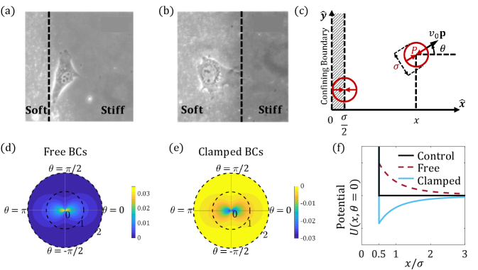
Figure 1: Experimental motivation and model setup. (a, b) Isolated fibroblasts near interfaces between soft and stiffer regions of a polyacrylamide gel substrate (reproduced with permission from Ref. [17]). (a) A cell approaching the interface from the stiffer side (left) aligns parallel to the interface and remains in the stiffer region. (b) A cell on the softer side aligns normal to the interface and eventually crosses over to the stiffer side. (c) Schematic of a cell moving on a flat linear elastic substrate with uniform stiffness (given by Young’s modulus $E$, and Poisson’s ratio $\nu$) near a confining boundary. Clamped or free elastic boundary conditions are employed to distinguish between the cell being on the softer or stiffer region of the substrate, respectively. Unlike the experiment, the simulated cell is not allowed to cross the boundary. Traction forces generated by the cell are reduced to a contractile force dipole of strength ${\mathbf{P}}$ (red, inward pointing arrows) acting on the substrate. Cells are modeled as circular discs (shown here as red circles) of diameter $\sigma$. The direction of propulsion ${\mathbf{p}}$ is assumed to be along the cell dipole axis and makes an angle $\theta$ with the horizontal axis. The cell lies a horizontal distance $x$ from the boundary (the $y$ axis). An excluded region of extent $\sigma/2$ (a lower limit) at the boundary models confinement. (d,e) The spatial map of the elastic interaction potential experienced by the cell as a function of distance from the boundary and the orientation is shown for free and clamped boundaries, respectively. (f) The potential is plotted as a function of distance for the control case representing pure confinement without elastic interactions (solid black), the repulsive free boundary (dashed, brown) and the attractive clamped boundary (solid, cyan).

A complete description of durotaxis thus requires combining the dipole-based model for cell traction-induced matrix deformations by adherent cells, with an appropriate model for stochastic cell movement [37, 38, 39]. We consider here persistently motile cells that move in a directed manner for a characteristic time before reorienting. Since migrating cells generate protrusions that may be randomly driven by noisy internal signalling cues [40], the motion of our model cells feature stochastic reorientations and velocity fluctuations [9]. Cells are also known to actively modulate this stochasticity and thereby move persistently along the direction of their contractility, such that the polarization is along the dipole or principal traction axis [41]. We here propose and study a general, phenomenological model that incorporates these key elements to provide a statistical physics description of durotaxis.

Figs. 1(a) and (b), reproduced from Ref. 17, illustrate the scenario we wish to analyze theoretically. The authors here examined the behavior of a fibroblast cell cultured on a deformable polyacrylamyde hydrogel substrate, and located near an interface separating a soft region from a stiffer region. When the cell is on the stiff side, it aligns parallel to the interface and remains on the stiffer side. On the other hand, when the cell starts off on the soft side, it aligns perpendicular to the interface and eventually moves and crosses over to the stiffer side (not shown). This behavior may be understood by considering the polarized cell as a force dipole acting along its axis of elongation [36]. When on the stiffer side (Fig. 1(a)), the cell deforms the interface and the softer elastic medium on the other side of the interface can easily displace, resulting in an effectively stress-free boundary condition. Conversely, when the cell is on the soft side (Fig. 1 (b)), the rigid medium on the other side undergoes minimal displacement at the interface, resulting in an effectively clamped boundary. In fact, it was shown in Ref. [36] that when the interface acts as a clamped (free) boundary, the effective elastic interaction potential between a cell dipole and the interface computed by a full consideration of the virtual image stress distribution required to satisfy the relevant boundary condition, yields an attractive (repulsive) force on the dipole. Additionally, elastic interactions also result in a torque that orients the dipole perpendicular (parallel) to the interface.

While this static model for an adherent cell provides a heuristic explanation for single-cell durotaxis [36], we consider here the role of cell motility, in the presence of such an elastic boundary interaction arising from cell traction. Unlike the original durotactic experiment [17], we also choose to confine the model cell to either the softer or stiffer region. This mimics complex or micro-patterned environments and allows us to study the interplay of motility,confinement and elastic interactions. The model setup of a cell moving on an elastic substrate near a confining boundary is illustrated in Fig. 1c. The substrate deformation-mediated elastic interaction potential experienced by a stationary cell is depicted in Figs. 1 (d)-(f). The elastic potential as a function of the cell orientation is shown for free and clamped boundaries in Figs. 1(d) and (e), respectively. These highlight the repulsive and attractive nature of the interactions, as well as the favored parallel and perpendicular orientations. Fig. 1(f) shows the long-range spatial decay of the potential away from the interface in the clamped, free and “control” regions, the latter corresponding to only steric interactions with the confining boundary. Using this model setup, described in more detail in the next section, we seek to predict how statistical distributions of cells depend on the persistent and stochastic aspects of motility, as well as the strength and nature of the elastic interactions with the boundary. Fig. 1(e).

II Model for cell motility and elastic cell-boundary interactions

The motion of each cell is modeled using Langevin dynamics in the overdamped limit since inertial effects are negligible at the microscale. Each cell is treated as a disk of diameter of diameter $\sigma$ moving on a 2D $xy$-plane corresponding to the surface of an idealized, infinitely thick elastic substrate. The state of each cell is defined by its position vector ${\bf r}$ corresponding to the cell center, and unit orientation vector ${\bf p}$ associated with its self-propulsion direction (Fig. 1(c)). Cells move with speed $v_{0}$ in the direction $\mathrm{\bf p}$ (with Cartesian components $(\cos\theta,\sin\theta)$), and interact with boundaries through a potential $U(x,\theta)$ that depends on the normal distance from the boundary $x$ (see Fig. 1 -(f)), and on the angle $\theta$ [36]. The equations that govern the dynamics of a cell modeled as an active Brownian particle in an elastic potential are,

$$\frac{\partial\mathbf{r}}{\partial t} = v_{\mathrm{0}}{\mathbf{p}}-\mu_{T}\mathbf{\nabla}U+\sqrt{2D_{T}}\bm{\eta}_{\mathrm{T}}(t),$$ (1)

$$\frac{\partial\theta}{\partial t} = -\mu_{R}\frac{\partial U}{\partial\theta}+\sqrt{2D_{R}}\eta_{\mathrm{R}}(t),$$ (2)

where $D_{R}$ and $D_{T}$ are diffusion coefficients associated with orientational and translational fluctuations of the cell’s principal axis and center of mass, respectively, while $\mu_{R}$ and $\mu_{T}$ represent the corresponding rotational and translational mobility. For passive bodies in an ambient viscous medium, these mobility coefficients depend on the medium’s viscosity and thermodynamic temperature, and are also coupled via the body’s geometry, through Stokes-Einstein relations [42, 43]. Living cells, however, being active and not at equilibrium, do not have to adhere to this constraint. Their self-propulsion velocity can be resolved into a persistent as well as a stochastic part, the latter arising from random protrusions created by cytoskeletal processes. Thus, in principle, the cell is free to set effective translational and rotational diffusivities, $D_{T}$ and $D_{R}$, independently. For migratory cells, mobility coefficients arise from dissipative frictional mechanisms at the cell-substrate interface. The friction can contribute additional terms due to memory and inertial effects in the cell dynamics [44], while the statistics of the cell trajectory may deviate from a persistent random walk [45] in 3D [46], effects which we ignore here for simplicity. We include the effects of stochastic noise via the last terms on the right hand side of Eqs. (1) and (2), $\bm{\eta}_{\mathrm{T}}(t)$ and $\eta_{\mathrm{R}}(t)$ respectively, and correspond to white noise.

The boundary interaction potential $U$ includes contributions from cell-boundary interactions mediated by the underlying elastic substrate, and an additional short-range steric interaction term that prevents cells from penetrating the boundaries. Exact implementations of this steric interaction will be discussed later. The elastic potential arising from the interaction of the cell force dipole with the substrate deformation (strain) it generates in the vicinity of the free or clamped boundary is of the form [35],

$$U(x,\theta)=-\left(\frac{P^{2}}{256\pi E}\right)\frac{f_{\nu}(\theta)}{x^{3}},$$ (3)

where $P$ is the strength of the cellular force dipole that is aligned with the cell major axis, parallel to the direction of motility ${\bf p}$, and $f_{\nu}(\theta)=(a_{\nu}+b_{\nu}\cos^{2}\theta+c_{\nu}\cos^{4}\theta)$ encodes the angular dependence of the potential $U$ that is separable in $x$ and $\theta$ coordinates. Substrate elastic properties affect the potential $U$ through its dependence on the Young’s modulus $E$, and the Poisson’s ratio $\nu$.

Specifically, the angular factor $f_{\nu}(\theta)$depends on the substrate Poisson ratio via constants $a_{\nu}$, $b_{\nu}$ and $c_{\nu}$ (see Appendix A). Importantly, the constants vary depending on the type of boundary condition - i.e., whether the boundary is free or clamped. Exact forms of these from Ref. [35] are provided in Appendix A.

The spatial dependence of the potential may be rationalized as follows. The cellular force dipole exerted by the cell interacts with local deformation arising due to the presence of the boundary. This strain field is generated by the associated “image” dipole configuration required to satisfy the free or clamped condition on the boundary [47]. The strain created by a dipole in an elastic half-space decays with distance as $~{}1/x^{3}$, while it is linear in the magnitude of the dipole moment, $P$. The dipole-dipole interaction potential therefore scales as $P^{2}/x^{3}$. In writing down equations Eqs. (1), (2) and (3), we made a simplifying assumption, valid for highly polarized cells such as fibroblasts, by identifying the dipole axis with the direction of motion [28, 38]. The coarse-grained model of cell traction force distribution as a force dipole is a far-field approximation, valid when the cell-boundary distance is greater than the cell diameter.

Our model features four dimensionless parameters controlling cell trajectories:

$$Pe \equiv\frac{v_{\mathrm{0}}}{D_{R}\sigma},\>A\equiv\frac{1}{50}\left(\frac{\mu_{T}P^{2}}{ED_{R}\sigma^{5}}\right),\>B\equiv\frac{1}{50}\left(\frac{\mu_{R}P^{2}}{ED_{R}\sigma^{3}}\right),$$ (4)

$$D \equiv{D_{T}\over D_{R}\sigma^{2}}.$$

The Péclet number $Pe$ quantifies the relative importance of directed self-propulsion and random motion, and is a measure of persistent motion of the particles in the absence of boundary potential $U$. Parameter $A$ quantifies the strength of the force, while $B$ quantifies the strength of re-orienting torque, both acting on the cell due to cell-boundary elastic interactions. Both parameters depend on the elastic properties of the substrate but are notably independent of active self-propulsion. The factor of $50$ in the definition of $A$ and $B$ results from the angular average $\langle f_{\nu}(\theta)\rangle\equiv(1/2\pi)\int_{0}^{2\pi}f_{\nu}(\theta)d\theta=1/50$. In this work, we set the substrate Poisson’s ratio to a representative value of $\nu=0.3$ [17, 48].

In general, $A$ and $B$ can differ in value depending on the specific mode of cell migration. The ratio $A/B$ is equivalent to ($\mu_{T}/\mu_{R}\sigma^{2}$). For a passive spherical particle at equilibrium in a viscous medium, the ratio $A/B=1/3$. For elongated rod-like objects, the ratio depends on the aspect ratio and tends to $1/9$ in the limit of infinitesimally thin rods [49, 50, 51]. The case of cells on an elastic substrate is more complex. The values of $A$ and $B$ can strongly depend on the internal mechanisms driving cell motility, an example being internal changes in cell biochemistry that determine the direction of protrusions in the cells.

To estimate $A$ in cell culture experiments, we use the typical value for the traction force of a contractile cell adhered to an elastic substrate $F\sim 10-100$ $\mathrm{n}\mathrm{N}$, with a distance of $\sigma\sim 10-50$ $\mu\mathrm{m}$ separating the adhesion sites. This results in a force dipole moment for a single cell, $P=F\cdot\sigma\sim 10^{-12}-10^{-11}$ $\mathrm{J}$ [35]. Using typical values of substrate stiffness in durotaxis experiments, $E\sim 10$ $\mathrm{k}\mathrm{P}\mathrm{a}$ [23], rotational diffusion, $D_{R}\sim 10^{-2}$ $\mathrm{m}\mathrm{i}\mathrm{n}^{-1}$ [30], cell size $\sigma\sim 20$ $\mu\mathrm{m}$, and previously estimated translational mobility [52], $\mu_{T}\sim 0.1\,\mu\mathrm{m/min}\cdot\mathrm{pN}^{-1}$, we estimate $A\sim 1$. By changing substrate stiffness and allowing for variation in cell types, we estimate a typical range of $A\sim 0.1-10$, where $A$ can be small on very stiff substrates. Further using $\mu_{R}\sim 10^{-4}$ $\mu\mathrm{m}^{-1}\mathrm{m}\mathrm{i}\mathrm{n}^{-1}\mathrm{p}\mathrm{N}^{-1}$, we estimate $B\sim 1$. We again estimate a typical range of $B\sim 0.1-10$ by changing the substrate stiffness, where $B$ is small on high substrate stiffness.

We estimate $Pe\sim 0-10$ based on typical cell migration velocities [30], $v_{0}\sim 0-100$ $\mu\mathrm{m}\mathrm{/}\mathrm{h}\mathrm{r}$. We choose to keep the parameter $D=(D_{T}/D_{R}\sigma^{2})$ fixed at $0$ or $1$ in our simulations. The former simplifying choice corresponds to the regime of highly persistent cell migration characterized by high $Pe$ values, where the effective translational diffusion results from cell reorientations, and is given by $\ v_{0}^{2}/D_{R}$. We also fix the size of the simulation box to $L=40\sigma$.

III Results

III.1 Elastic interactions determine steady state distributions near clamped and free elastic boundaries

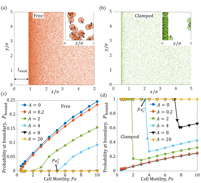
Figure 2: Spatial probability density profiles of motile dipole cells near free, and near clamped elastic boundaries. Distribution of particles as distance from the boundary is plotted as scatter plot for (a) free ($A=B=16$, $Pe=8$), and for (b) clamped boundaries ($A=B=8$, $Pe=8$) with insets showing motile cells. Cells can interact sterically with each other and some overlap is permitted. In (a) the repulsive potential from the free boundaries results in void region of extent $\ell_{\mathrm{void}}$ which particles cannot occupy or populate. Particles close to the boundary are oriented parallel to the boundary due to elastic realignment torques (see also inset. In (b) we show snapshots in the case of a clamped boundary. The interface is attractive, and particles localize at the boundaries compared to the bulk. Additionally, the elastic torque from the clamped boundaries orients the particles orthogonal to the boundary (see inset in (b)). (c,d) We quantify the localization of particles at the free (c) and clamped (d) boundaries as a function of $Pe$ for various values of $A(=B)$. (c) For free boundaries, the localization at the boundary decreases with $A$. The value of $P_{\mathrm{bound}}$ increases with $Pe$ due to persistence driven accumulation at the boundary. At very high $A$, the particles cannot get close to the boundary leading to $P_{\mathrm{bound}}=0$. $Pe^{*}_{f}$ corresponds to the critical value of $Pe$ at which the cell’s motility can overcome the repulsive boundary force and reach the boundary at any specific value of $A$. $Pe^{*}_{f}$ increases with $A$ (only shown for $A=4$). (d) In case of clamped boundaries, the localization at the boundaries increased with $A$. At low $A$, the boundary probability $P_{\mathrm{bound}}$ increases with $Pe$, since particles have a higher tendency to encounter the boundary. At higher values of $A$, the particles stay at the boundary until reorientation events occurs. The high speed (high $Pe$) leads to rapid escape, resulting in a sharp drop in $P_{\mathrm{bound}}$. There is further increase in $P_{\mathrm{bound}}$ due to persistence driven accumulation. At very high $A$ the particles don’t leave the boundary leading to $P_{\mathrm{bound}}=1$. Here, $Pe^{*}_{c}$ corresponds to the critical value of $Pe$ at which the cell’s motility can overcome the attractive boundary force and populate the bulk at any specific value of $A$. We notw that $Pe^{*}_{c}$ increases with $A$, here we show the trend $A=4$).

Theoretical models describing the statistical behavior of active particles under confinement have been studied extensively in earlier works that compute the density, surface density, polarization, and orientation distributions of active particles between two parallel confining boundaries or at straight or curved boundaries [53, 54, 55, 56, 57]. These studies show that statistical steady state distributions depend strongly on particle activity, the shape of the particles, and the curvature of the boundaries. Passive particles moving in a constant temperature, non-deforming medium without persistent self-propulsion ($Pe=0$), are expected to reach thermodynamic equilibrium and have uniform distribution between the boundaries that maximizes entropy. In contrast, as $Pe\to\infty$, particles populate the boundaries at all times with the probability of finding particles at the boundary tending to unity resulting in a diverging surface density. The surface density also depends on the curvature of the surface, and specifically on whether it is concave or convex shaped [58].

Cell-boundary interactions mediated by an ambient material medium have also been investigated in detail for a related class of problems – the interaction of low Reynolds number microswimmers such as bacteria, algae and sperm with boundaries [59, 60, 61, 62, 63, 64, 65, 66, 67, 68, 69]. Unlike the cells studied here that act as contractile dipoles, free swimming organisms can act as pushers (bacteria, and sperm) or pullers (algal cells). Far from interfaces, pushers generate extensile force dipoles on the ambient fluid, while pullers exert contractile force dipolar stresses. Additional stresses on the fluid are generated in pushers due to “rotlet” dipoles arising from counter-rotation of the cell body and the flagellar bundle. The presence of interfaces near swimming cells results in wall induced forces and torques on these swimmers; these effects arise due to the requirement that the overall fluid fields generated by the moving cells, and mediated by the interface(s), satisfy appropriate boundary conditions – that is no-slip for solid walls, or stress-free for free surfaces.

Experimental studies on swimmers near surfactant-free, solid, no-slip surfaces indicate that, irrespective of the type of dipolar swimmer, microorganisms tend to accumulate near the interface albeit with varying orientations. Pushers tend to align parallel to no-slip solid interfaces due to hydrodynamic torques, and swim along the surface exhibiting long residence times [59, 67]. Analyzing the competition between cell-wall hydrodynamic attraction and rotational diffusion, Drescher et al. estimated characteristic cell-wall interaction time scales and deduced that hydrodynamic wall-induced attraction dominates provided the distance from the wall $x<P(a/v_{o}D_{R})$ where $\sigma$ is the cell (body) size, $P$ is the hydrodynamic dipole strength, and $v_{0}$ is the self propulsion speed. Contractile pullers meanwhile have been observed to align perpendicular to the interface and remain trapped until they can reorient and escape due to thermal noise or rotational diffusion arising from variations in the swimming mechanism [59]. Interestingly, pushers are found to be always attracted to surfactant-free (clean) interfaces with the Stokes dipole oriented and aligned parallel to the interface, for both free surfaces as well as for solid walls [67, 65].

In this work, we investigate the effects of cell-interface elastic and steric interactions on the surface and bulk distributions of active particles representing motile cells on elastic substrates. Motivated by the process of single cell durotaxis across sharp gradients of substrate stiffness as shown in Figs. 1a , we study the effect of elastic forces and torques on the density and orientational distributions of motile cells at the confining boundary. We carry out simulations of cell trajectories using the model Eqs. 1-2 for a range of values of self-propulsion, $Pe=0.5-10$, and elastic interaction, $A(=B)=0$ to $20$, that were estimated in the model section for cell culture experiments. From these simulations, we compute the probability of finding a particle at the boundary using $P_{\mathrm{bound}}=N_{\mathrm{bound}}/{N_{\mathrm{total}}}$, where $N_{\mathrm{bound}}$ is the total number of times a particle is at the boundary – that is, its center is located at $x=x_{b}\equiv\sigma/2$ after the instantaneous displacement/reassignment step (Appendix C). ${N_{\mathrm{total}}}$ meanwhile is the total number times the particle is observed. To aid in the analysis and interpretation of results, we set $D=0$, that is switch off translational diffusivity $D_{T}=0$, in our simulations. In the short time limit relative to the persistence time $D_{R}^{-1}$, this allows cells to localize and stay at the boundary except when they self-propel. Over longer times however, an effective diffusivity that is $v_{0}^{2}/D_{R}$ arises due to the combination of self-propulsion and re-orientations represented by rotational diffusion.

As a point of departure, we first describe the results in the absence of elastic interactions with the boundary, $A=B=0$. Geometric confinement prevents cells from leaving the system in the direction normal to the boundaries. Consistent with previous studies on non-interacting Active Brownian Particles (ABPs) [53], we observe localization of cells at the boundaries, with the associated number densities at the boundaries ($N_{\mathrm{bound}}$) increasing with the Péclet number ($Pe$). To rationalize this, we note that increasing Péclet number is equivalent to faster cell migration speed and more persistent motion (Fig. 2 (c), (d)). Cells are able to translate over longer distances due to decreased effects of diffusion. Once the cells reach the boundaries however, they tend to remain there since they are oriented towards the wall, until reorientation is caused by rotational diffusion over the characteristic timescale $\sim D_{R}^{-1}$. Upon reorientation, the cell’s orientation given by the polarization vector’s angle $\theta$ is pointed away from the boundary, and its self-propulsion enables escape and movement into the bulk. Increasing cell Péclet number decreases the time spent between the confining boundaries which in turn increases their probability to be at the boundary.

Such localization at the boundary, while well-known for microswimmers as previously described and also for synthetic active particles, is yet to be demonstrated for crawling animal cells. We propose that this effect may be detected by tracking spatial probability of cells in a dilute cell culture experiment where confinement is created by micro-patterning the underlying elastic substrate into two discrete regions, only one of which favors adhesion. The interface between these two regions will act as a confining boundary that restricts cell migration into the unfavorable region where cells cannot adhere. Henceforth in this work, we term this increased localization of cells at the confining boundary by purely kinetic means, motility-induced accumulation (MIA).

The probability of a cell being at the boundary is strongly modulated by the nature of elastic interactions in our model. Specifically, the sign of elastic interaction depends on the type of boundary condition, clamped (i.e. “zero displacement”) or free (i.e., “zero stress”). For stress-free boundary conditions representing an interface with a softer substrate, increasing repulsive forces act on the cells as they approach the boundary. Therefore in this case, cells are unable to reach the boundary and remain a distance away from it, see Fig. 2(a). Furthermore, the torque from the elastic interaction induces cells close to the boundary to align parallel to it, see inset to Fig. 2. Increasing the interaction parameter $A$ (here we set $B=A$) increases the length of the region over which the repulsive force acts and reduces the probability of a cell being at the boundary. For $A>0$ and low $Pe$, there is no localization at the boundary, Fig. 2(c). Quantifying this localization by a probability density of observing particles at the boundary we find from our simulations that for each value of $A$, there exists a critical Péclet number $Pe_{\mathrm{f}}^{*}$ at which the localization probability, $P_{\textrm{bound}}$ at the boundary becomes non-zero. For $A>0$, increasing the Péclet number to values larger than $Pe_{\mathrm{f}}^{*}$, increases the probability of the cells to localize at the boundary. When $Pe<Pe_{\mathrm{f}}^{*}$, cells cannot reach the boundary resulting in a void region evident in Fig. 2 (a). We find that $Pe_{\mathrm{f}}^{*}$ increases with the interaction parameter $A$. This increase is expected to be linear from force balance.

The situation is quite different for cells interacting with clamped boundaries. In this case, cell-boundary elastic interactions are attractive and increasing $A$ localizes more cells at the boundary, Fig. 2(b). In addition, the elastic torque from the boundary orients cells orthogonal to the boundary, seen in Fig. 2(b) (inset). At low values of $A$ (for $A<2$), we find that $P_{\mathrm{bound}}$ increases monotonically with $Pe$. This is a consequence of the enhanced flux towards the boundary due to the higher speed ($Pe$), and the attractive potential that traps the cells. For higher $A$ ($A>2$), and at low $Pe$, cells are strongly localized at the boundary with $P_{\mathrm{bound}}=1$ due to the strongly attractive elastic force from the clamped boundary. For $Pe\geq 1$, we see a reduction in $P_{\mathrm{bound}}$ as escape from the boundary is increasingly facilitated by the greater speed. The critical Péclet number $Pe_{\mathrm{c}}^{*}$ at which the cells overcome the attractive interaction with the clamped boundary and escape into the bulk increases with $A$ and is expected to be linear from force balance. Eventually however as $Pe\gg 1$, the role of the elastic potential becomes subdominant to the effects of increased motility, and particles are more likely to be observed at the boundary than in the bulk. In contrast, for a clamped elastic boundary, when the strength of the elastic attraction $A$ is sufficiently larger than the persistent cell motility $Pe$, $P_{\mathrm{bound}}=1$ implying cells are strongly localized at the boundary. These cells have a higher chance of crossing over to the stiffer side. On the other hand, an elastic free boundary decreases $P_{\mathrm{bound}}$ thereby reducing the cells’ tendency to go towards the softer substrate. Both these types of interactions from clamped and free boundaries, while distinct, promote durotaxis. On the other hand, higher cell migration speeds promote their motility-induced accumulation at a confining boundary without discriminating between stiffer and softer substrates.

III.2 Free elastic (repulsive) boundary induces depletion

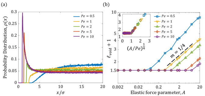
Figure 3: Depletion region near a free boundary, and its dependence on motility and elastic strength interaction parameters. (a) The probability distribution $\rho(x)$ of a particle is plotted as a function of closest distance $x$ from the boundary for $A=20$ with $Pe=0.5,1,2,5,10$. Increasing $Pe$ leads to a reduction in the length of the void region. (b) The void length scales as $A^{1/4}$, and $Pe^{-{1/4}}$ (for constant $A$) as predicted from force balance,see Eq. (5). Inset shows the collapse of the $\ell_{\mathrm{void}}+1$ vs $\left(A/Pe\right)^{1/4}$ for $Pe=0.5,1,2,5,10$.

We have demonstrated that our simulated cells are repelled by the free boundary due to the nature of the elastic potential. We track the positions of all cells over time and establish the closest distance from the boundary accessed by each. We showed in Sec. IIA that the repulsive force from the free boundary induces a effective void region where cell do not penetrate, see Fig. 2(a). To characterize this void region systematically, we plot the statistically attained (time averaged and ensemble averaged for all cells ) probability distribution function $\rho(x)$ as a function of $x$ (the distance from the boundary) for various values of $A$ and $Pe$. To obtain $\rho(x)$, we simply record the positions of the cells after sufficient time required to reach steady state has elapsed. The length of the void region $\ell_{\mathrm{void}}$ is evaluated through these distributions, and is measured as the minimum distance at which the spatial density attains a non-zero value. For fixed values of A (for instance, $A$=20 in Fig. 3 - (a)), we find that increasing $Pe$ decreases the length of the void region. In general, increasing $A$ increases $\ell_{\mathrm{void}}$ while increasing $Pe$ decreases it.

We estimate $\ell_{\mathrm{void}}$ for $Pe$ from $0.1$ to $10$ and for $A=B$ from $0.002$ to $20$ to discern trends from physical scaling. Consider the balance of forces acting on a cell located at $x=\ell_{\mathrm{void}}$. Balancing the self-propulsion ($\sim Pe$) and elastic interaction forces ($\sim A/(x/\sigma+1)^{4}$) that move the cell, we obtain (see also Eq. (17)),

$$(\ell_{\mathrm{void}}/\sigma)+1\sim\left({A/Pe}\right)^{\frac{1}{4}}.$$ (5)

Indeed, void lengths extracted from simulated probability distributions confirm this theoretically predicted scaling in Fig. 3(b). Experimentally, the presence of a void region may be detected by culturing and tracking cells on a stiff adhesive region of an elastic substrate, adjoining a very soft, non-adhesive region that acts as a free boundary. Our model predicts low probability of finding cells in a void region.

III.3 Clamped (attractive) boundary: trapping and motility-assisted escape ($Pe>A$) by reorientation

The clamped boundary condition corresponds to the cell being on the softer substrate in our model. It facilitates durotaxis by inducing an attractive force and aligning torque on the cellular force dipole. However, cells have a finite probability to escape from this attractive confinement at the boundary, by reorienting through random internal fluctuations in cell polarity, and migrating away, provided that $Pe\gtrsim A$. When $A\geq 1$ and $Pe\sim 1$, cells tend to localize at the clamped boundary, as seen in Figs. 2(b) and (d). On the other hand, a large elastic torque, $B\geq 1$, orients the direction of propulsion directly towards or away from the boundary, as shown in the schematic Fig. 4(a).

We now quantitatively investigate the rate at which the cells trapped at the boundary flip their orientation from pointing towards the boundary to pointing away from the boundary. Such a calculation will help us estimate the time scale over which escape of trapped cells is possible. Since reorientation dynamics is dominated by the boundary-induced elastic torque, we focus on $B$ as our parameter of interest in this subsection. Since escape after rotation diffusion-enabled reorientation is possible through persistent motility alone when $Pe>A$, we continue to keep the translational diffusion parameter $D=0$ in this section.

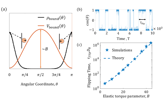
Figure 4: Cell reorientation (flip) kinetics at clamped (attractive) boundary quantified by barrier crossing theory. (a) For a clamped boundary, and at very high values of $A$ and $B$, cells localize at the boundary even at high values of $Pe$, and are oriented perpendicular to the boundary. (b) Rotational diffusion enables the cell to transition from the parallel to the anti-parallel configuration. These random flips are recorded for a cell stuck at the boundary for $A=B=20$. (c) The average frequency of these flips is observed as a function of $B$. The flipping time follows Kramer’s theory of barrier crossing and is given by Eq. (6).

As depicted in Fig. 4(a), cells can reside in one of two possible states given by the minima of the potential well $U(x=x_{b},\theta)$. It can switch randomly from one state to the other. Flips are defined as these large reorientation events when $\theta$ changes from $\pi$ to $0$ or vice versa. To estimate the frequency of flips, we track the change in orientation of cells localized at the boundary, given by the angle $\theta$, see Fig. 1(c). Thus, flips result in change in sign of $\cos{\theta}$ , seen in Fig. 4(a). A typical simulation trajectory in Fig. 4(b) shows that flipping occurs multiple times during a given simulation run, even at high values of $B$. We measure this effect as a flipping time $\tau_{\mathrm{flip}}$ for a cell, which is the residence time of the cell in either state. Following the orientation of a single cell over the time it is trapped at the boundary provides a distribution of flipping times. Here we specifically calculate the mean flipping time $\tau_{\mathrm{flip}}$ for all cells for $B$ ranging from $4$ to $45$ with $A$ set to equal $B$. The results in Fig. 4(c) show that $\tau_{\mathrm{flip}}$ increases with $B$. The dependence of $\tau_{\mathrm{flip}}$ with $B$ may be analytically determined from Kramer’s theory of barrier crossing [70] and has the form,

$$\tau_{\mathrm{flip}}=\frac{2\pi}{\mu_{R}\sqrt{U^{\prime\prime}(0)|U^{\prime\prime}({\pi/2})|}}\exp{\left(\mu_{R}\frac{U({\pi/2})-U(0)}{D_{R}}\right)}\sim\frac{1}{B}\exp{\left(-B\frac{(b_{\nu}^{c}+c_{\nu}^{c})}{864\pi}\right)}.$$ (6)

where we used the form of the elastic potential $U(x,\theta)$ given in Eq. 3. Note that since our simulation is for cells trapped at the boundary that are free to change orientation, the potential $U(x,\theta)$ is evaluated at a fixed value of $x=\sigma/2$. The theoretically predicted flipping times from Eq. 6 (dashed line) closely agree with the simulation data in Fig. 4(c).

In the limit of very large $B$, cells at the boundary are always oriented orthogonal to the boundary, either oriented away or towards it, as seen in the schematic Fig. 4(a). For low values of $B$ however, cells may adopt other orientations. To study this, we calculate in Fig. 5 the orientational probability density $\rho_{\mathrm{bound}}(\theta)$ of the cells at the boundary for $B(=A)$ equal to $0.2$ and $2$. At $A=B=0.2$, Fig. 5(a), both force and torque from the elastic interactions with the boundary are low. Cells pointing away from the boundary with $\cos{\theta>0}$ are no longer strongly attracted by the boundary and may escape by self-propulsion. The angle at which these cells lose contact with the boundary, defined here as $\theta_{\textrm{esc}}$, is then the minimum angle at which $\rho_{\textrm{bound}}(\theta)$ just becomes non-zero. In the case of $B=A=0.2$, this escape angle is close to, but smaller than $\pi/2$. Increasing $Pe$ increases the $\theta_{\textrm{esc}}$ slightly towards $\pi/2$, as shown in the inset to Fig. 5(a).

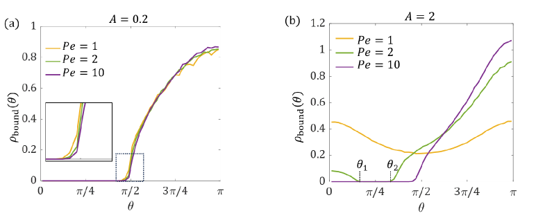
Figure 5: Orientational probability profiles of cells at clamped boundary provides bounds for escape. The angular probability distribution at the boundary $\rho_{\mathrm{bound}}(\theta)$ is plotted for $A=0.2$ and $A=2$. Here we set $B=A$ in both cases. (a) For $A=0.2$, cells are weakly attracted by the boundary and since $B=0.2$, the torque due to elastic interaction is low. Under these conditions $\rho_{\mathrm{bound}}(\theta)>0$ when cells are oriented towards the boundary. Increasing the $Pe$ increases the angle through which the cell can escape from the boundary (inset (a)). $\theta_{\textrm{esc}}$ is observed to be $77.4^{0}$, $81^{0}$ and $84.6^{0}$ for $Pe=1$, $2$ and $10$ respectively. (b) When $A=B=2$, we identify 3 distinct regimes that are $Pe$ dependent. For $Pe=1$, the cells are stuck to the boundary but free to reorient due to rotational diffusion, preferentially orthogonal to the boundary. At $Pe=10$ the cells can escape the boundary forces when the cell is oriented away from the boundary. At $Pe=2$, the cells are only able to escape when their orientation lies in the angular pocket between $\theta=0$ and $\pi/2$, denoted by dotted lines at $\theta_{1}=30.7^{0}$ and $\theta_{2}=55.8^{0}$.

The orientational probability density $\rho_{\mathrm{bound}}(\theta)$ is controlled by the elastic torque which induces cell alignment orthogonal to the boundary. For moderate values of $B$, such as when $B=A=2$, we observe three distinct regimes separated by two transition Péclet numbers, $Pe_{1}$ and $Pe_{2}$, as seen in Fig. 5(b). For low values of $Pe\leq Pe_{1}$, the elastic attractive force from the boundary, given by $A$, is strong enough to prevent cell escape, even when the cell is oriented away from the boundary. At high Péclet number, $Pe>Pe_{2}$, cells are able to escape the boundary interactions provided the orientation angle $\theta<\theta_{\textrm{esc}}$, where $0<\theta_{\textrm{esc}}<\pi/2$. As $Pe$ increases from $2$ to $10$, we see that the angular pocket (or the range in angular coordinates) required for escape, increases.

In these simulations without translational diffusion ($D=0$), a cell can escape from the boundary only if the attractive force from the boundary is overcome by the normal component of its self-propulsive force. In the intermediate motility regime corresponding to $Pe_{1}<Pe<Pe_{2}$, cells may escape only when their orientation lies between $\theta_{1}$ and $\theta_{2}$ (here, $0\leq\theta_{1}\leq\theta\leq\theta_{2}<\pi/2$). The transition Péclet numbers $Pe_{1}$ and $Pe_{2}$ are determined by balancing the $x$-component of the self-propulsive force (that is proportional to $Pe$) with the elastic force at the boundary. Evaluated at the boundary position, $x=x_{b}=\sigma/2$, this force balance takes the form

$$Pe\cos\theta=\frac{3A}{\left(x_{b}/\sigma+1\right)^{4}}\tilde{f}_{\nu}(\theta)$$ (7)

where $\tilde{f}_{\nu}(\theta)$ is the rescaled form of $f_{\nu}(\theta)$ in Eq. 3, defined as $\tilde{f}_{\nu}(\theta)\equiv\frac{50}{256\pi}f_{\nu}(\theta)$, such that $\tilde{f}_{\nu}(\theta)\sim 1$. The values of $Pe_{1}$ and $Pe_{2}$ are then evaluated using the orientation probability distributions (see Appendix D). From these, the region of escape in $\theta$ can be readily identified. When $A=2$, we find $Pe_{1}=1.82$ and $Pe_{2}=2.14$, respectively. When $A=0.2$, we estimate $Pe_{1}$ and $Pe_{2}$ to be $0.182$ and $0.214$ respectively. These values explain our simulation results in Figs. 5. In Fig. 5a, for $B=A=0.2$, all the three curves shown correspond to $Pe>Pe_{2}$, and can escape only below $\theta<\theta_{\textrm{esc}}$. In Fig. 5b, for $B=A=2$, all the three regimes discussed above are visible.

If the elastic force from the boundary is very strong, i.e., $A\gg Pe$ the cells cannot escape the influence of the boundary and will eventually show durotaxis. Since cell migration is stochastic and not deterministic, they can sometimes go opposite to the durotactic direction. This is possible in our model through an escape from the elastic attraction. This is likelier when the gradient in substrate stiffness is small, such that the boundary attractive force and the cell’s active propulsive force are comparable. The rotational diffusion in our model corresponds to random protrusions and internal chemical signaling that can reverse the polarization of the cells, while the propulsion drives them away from the boundary. Our predictions for the orientational distribution and dependence of reorientation (flipping) timescales may be checked in experiment by tracking the orientation and polarization (i.e. the direction of migration) of cells cultured on elastic substrates. How these quantities depend on on $A$ and $Pe$ may be checked by performing experiments on substrates of varying stiffness and quantifying cell traction (related to $A$) and migration speed (related to $Pe$).

III.4 Clamped (attractive) elastic boundary: escape facilitated by random translational protrusions ($Pe<A$)

In the previous section, we derived conditions for the motility-enabled escape after re-orientation of a cell away from the clamped boundary at which it was trapped. Our analysis of flipping dynamics and analytical prediction of the relevant time scale allows us to predict the first part of the overall escape process - i.e., the cell switching to a configuration favourable for escape, and concomitant conditions on $Pe$ for cells to leave the boundary.

Now, we consider the situation where random protrusions enable translational motion of the cell away from the attractive clamped boundary. Such protrusions, when large and frequent, lead to random movements of the cell center of mass, that has to be taken into account through non-zero values of the translational diffusion co-efficient, which we now set $D=D_{T}/D_{R}=1$. We extend our analysis and derive analytical expressions for the time required for cells to escape from the boundary to a dimensionless length-scale $L_{\mathrm{esc}}\gg 1$. This corresponds to a distance far enough from the potential well at $x=0$, where the torque and force arising from boundary interactions are negligible relative to random noise.

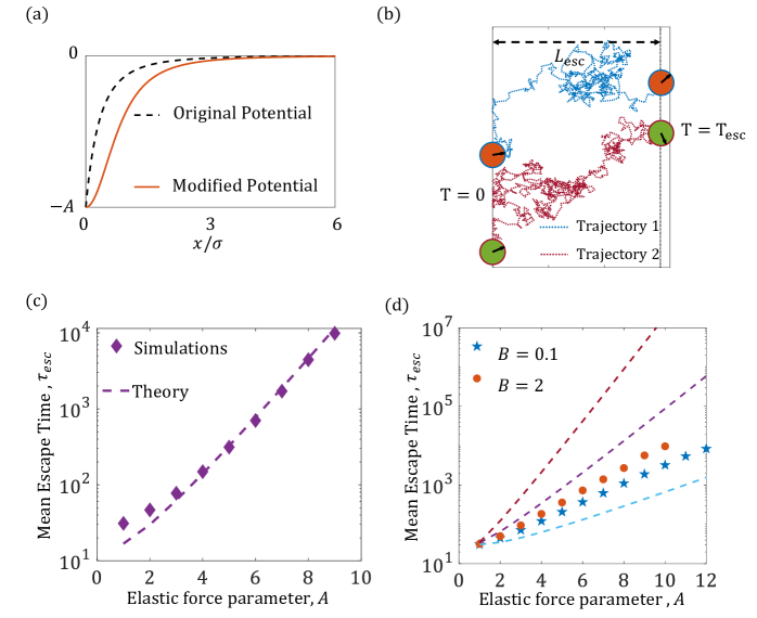
Figure 6: Diffusive escape from clamped boundary is governed by modified Kramers’ theory. (a) The angle-averaged original potential (black, dashed),given by Eq. (3), is modified to a form (orange, solid), given by Eq. (8), that introduces an analytical minimum at the boundary ($x=0$), thus making the potential amenable to analysis in terms of barrier crossing theory. The potential at the boundary is equal for both cases, and importantly the long range asymptotic form is the same for both. (b) cells are initialized at the boundary ($x=0$) at time $T=0$ with random orientations. Trajectories are then followed, until the cell reaches a position $x/\sigma=L_{\mathrm{esc}}$, upon which it is assumed to have escaped. The escape time $T=T_{\mathrm{esc}}$ is calculated for each cell trajectory when they cross the escape length for the first time. In the simulations we choose $L_{\mathrm{esc}}=6$. A distribution of first passage times is obtained from which the average escape time $\tau_{\mathrm{esc}}=\langle T_{\mathrm{esc}}\rangle$ is calculated. (c) Average (mean) escape time is plotted for a simplified 1D potential which is orientation angle independent. We observe that the results follow a modified version of Kramer’s theory given by Eq. (9) for $\tilde{f}_{\nu}(\theta)=1$. (d) $\tau_{\mathrm{esc}}$ for the 2D potential with both spatial and orientation dependence is plotted vs $A$ at $B=0.1$ and $2$. The dashed lines represent the analytical escape times (purple, for $\tilde{f}_{\nu}(\theta)=1$), escape along the direction of least resistance (light blue, escape along $\theta=\pi/2$) and escape along the direction of maximum resistance (brown, escape along $\theta=0$ or $\pi$). At $B=0.1$, torque is low and rotational diffusion aligns the cells in random directions but cells also prefer to escape along the direction of least resistance. At $B=2$, the escape time of cells is shifted towards escape along maximum resistance.

To aid the analytical derivation of the escape time from barrier crossing theory and enable comparison with our simulation results, we initialize our cells at a position corresponding to the local minimum in a potential $V$ satisfying the constraints $\partial V/\partial x=0$ and $\partial^{2}V/\partial x^{2}>0$ at $x=0$. This is done by modifying the functional form of the elastic potential while taking care to not change the long range behavior at $x\gg 1$ (see Fig. 6-a). This modified potential has a local minimum at the boundary as required for fidelity and consistency:

$$V(x,\theta)=-\frac{A}{((x/\sigma)^{2}+1)^{3/2}}\tilde{f}_{\nu}(\theta).$$ (8)

When $x/\sigma\sim L_{\mathrm{esc}}$, the magnitude of the potential is significantly lower than at the boundary. This furnishes the constraint that needs to be satisfied for escape, $A/L_{\mathrm{esc}}^{3}\ll 1$ (Fig. 6-a, b). Thus complete escape from the boundary is achieved if a cell starting at the boundary is able to leave the region $x/\sigma<L_{\mathrm{esc}}$ (Fig. 6-b).

The potential in Eq. (8) is used to obtain asymptotic estimates of the escape time, and also to investigate escape dynamics in our simulations. To allow for accurate statistics, we tracked $N=10^{4}$ cells in this potential for various values of $Pe$, $A$, and $B$. The position and orientation were tracked for cells initialized at the boundary ($x=\sigma/2$) until they crossed $x/\sigma=L_{\mathrm{esc}}$ for the first time. This data was used to relate the probability of escape and the average time of escape $\tau_{\mathrm{esc}}$, to interaction parameters $A$ and $B$, and to the motility parameter $Pe$.

As a prelude to developing a theoretical expression for active barrier crossing in a 2D potential, we first evaluate the mean escape time $\tau_{\mathrm{esc}}$ for cells without persistent motility ($Pe=0$), that is when cell dynamics correspond to thermally diffusive particles. We further reduce the dimensionality of the problem by considering a potential that is independent of the orientation of cells, thus fixing the angular factor $\tilde{f}_{\nu}(\theta)$ to be a constant. This corresponds to a particle either maintaining a constant orientation $\theta$, or exploring all angles equally such that the angular factor averages out to unity. This reformulated problem is equivalent to a 1D escape problem of a diffusing particle in an external potential, here arising from cell-boundary elastic interaction. Adapting previous work on Kramer’s theory applied to a particle in a generalized Lennard-Jones potential [71] to our modified potential, we find that the average escape time increases exponentially with the interaction parameter $A$, as seen in Fig. 6-(c). Here, the theoretical curve is calculated from the expression for escape time given by,

$$\tau^{\mathrm{1D}}_{\mathrm{esc}}\simeq\frac{1}{D_{R}}\left({{L_{\mathrm{esc}}-A^{1\over 3}}\over\sqrt{A}}\right)e^{A\tilde{f}_{\nu}(\theta)}\qquad{\mathrm{for}}\>\>\>\>\frac{A}{L_{\mathrm{esc}}^{3}}\ll 1,$$ (9)

where the calculation is detailed in Appendix E. As shown in Eq. (39), the pre-factor of the rate of barrier crossing in this long-range power law potential differs from the classical Kramer’s theory. In our simulations, we choose $L_{\mathrm{esc}}=6$ such that $A/L_{\mathrm{esc}}^{3}$ ranges from 0.005 to 0.055, thus ensuring the validity of the approximation, $A\ll L_{\mathrm{esc}}^{3}$, required to obtain the asymptotic expression for mean escape time. The simulation results are consistent with theoretical predictions for all values of $A\geq 3$ reported in Fig. 6(c). The average escape time, $\tau_{\mathrm{esc}}$ is seen to increase exponentially with interaction parameter $A$.

Starting from the orientation-independent asymptotic calculation for $\tau_{\mathrm{esc}}$, we next proceed to incorporate the orientation dependence of the potential $U$, while still keeping $Pe=0$. The escape problem is now two-dimensional, being in $x$-$\theta$ space, and the dynamics of cell reorientation affects the trajectories and probability of escape. In Fig. 6(d), we compare the simulation results of mean escape time $\tau_{\mathrm{esc}}$ with the theoretical bounds corresponding to escape along the direction of least resistance (light blue, Eq. (9) corresponding to $\tilde{f}_{\nu}(\theta=\pi/2)=0.53$), escape along direction of maximum resistance (brown, Eq. (9) ) corresponding to $\tilde{f}_{\nu}(\theta=0)=\tilde{f}_{\nu}(\theta=\pi)=1.8$ and the effectively 1D result (purple, Eq. (9) corresponding to averaging out the angular degree of freedom, $\tilde{f}_{\nu}(\theta)=1$). Note that the force resisting escape corresponds to the attractive elastic force generated by the clamped boundary, which scales with the angular factor, $\tilde{f}_{\nu}(\theta)$. The elastic force and torque parameters, $A$ and $B$, are chosen from representative values in the range $A=1-12$, and $B=0.1,2$ respectively.

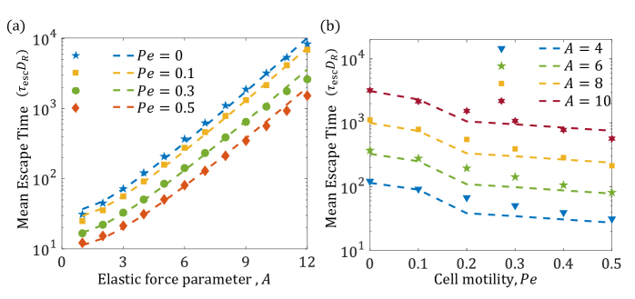
Figure 7: Self propulsion-assisted escape from the attractive clamped boundary (at fixed $B=0.1$). (a) The normalized mean escape time $\tau_{\mathrm{esc}}D_{R}$ in simulation for varying $Pe$ (shown by markers) follows the modified exponential relations in Eq. (13) with increasing $A$ (shown by dashed lines) by only fitting pre-factor $m(\mathrm{Pe})$ at the given range of values of $\mathrm{Pe}=0.1-0.5$. Here, we assume the coupling between position and orientation results in an effective value of $f^{*}=0.651$, which is determined from fitting values for 2D passive particles at the given value of $B=0.1$. The function $m$ is linear in the Péclet number and is found to be $m(Pe)=4.13-3.17Pe$. (b) Simulation results of the mean escape time (shown by markers) $\tau_{\mathrm{esc}}D_{R}$ for $A=4,6,8,10$ also follows the theoretical Ansatz, Eq. (13) (dashed lines) with $Pe$ based on the fitting pre-factor $m(Pe)$.

The two representative values of $B$ are chosen to highlight different regimes of orientation fluctuations during escape. In the low torque regime represented by $B=0.1$, cells can freely reorient due to rotational diffusion and tend to escape first along the angle that results in least resistive force from the boundary. However, constant fluctuations in their orientation cause them to deviate from this path. This leads to a higher $\tau_{\mathrm{esc}}$ than the theoretical prediction for the minimum resistance direction ($\theta=\pi/2$, light blue curve) in Fig. 6(d). However, the $\tau_{\mathrm{esc}}$ values remain below that given by the average of all orientations (brown). In the high torque regime, $B=2$, cells get aligned orthogonal to the boundary ($\theta=0$ or $\pi/2$ ) when they are close to it. They thus experience a stronger attractive force from the boundary, and have higher $\tau_{\mathrm{esc}}$ values, than in the low $B$ case. We do not report the cases when both $A$ and $B$ are high, because the mean escape times become too long to observe in our simulation time scale.

Motivated by the theoretical analysis for the 1D or angle-independent case, we now account for this effect of orientation fluctuations by assuming the Ansatz,

$$\tau^{\mathrm{2D}}_{\mathrm{esc}}\simeq{1\over D_{R}}m(B)\left({{L_{\mathrm{esc}}-A^{1\over 3}}\over\sqrt{A}}\right)\mathrm{e}^{Af^{*}(B)},$$ (10)

and estimating the functions $m(B)$ and $f^{*}(B)$ by fitting to simulation data. Here, we interpret $f^{*}(B)$ as a function of an effective weighted mean of the angle of escape of the cells, which corrects the deviation from the ideal 1D escape result. Thus, the function $f^{*}(B)$ quantifies the effect of coupling between the positional and orientational degrees of freedom on the effective energy landscape. The parameter $m(B)$ explicitly corrects for orientational effects on the frequency of possible escape trajectories, and thus on the escape time. By definition, for passive particles in 1D, $f^{*}=1$. The function $m(B)$ satisfies $m=1$ for the passive 1D case, and deviates from this value when $B>0$. Qualitatively, introducing the pre-factor $m(B)$ allows us to treat the full 2D escape problem as an appropriately averaged 1D escape problem.

Intuitively, we expect that self-propulsion helps particles escape from a confining potential. Thus our expectation is that $\tau_{\mathrm{esc}}$ is reduced for $Pe>0$ in comparison to $Pe=0$, as confirmed by the simulation results in Fig. 7. The effective potential barrier that the cell has to escape, modified now by its self propulsion velocity, can be written as [72]

$$\phi=\frac{Af^{*}}{({C_{1}}^{2}+1)^{3/2}}-\frac{Af^{*}}{({C_{2}}^{2}+1)^{3/2}}-Pe\left({C_{2}}-{C_{1}}\right).$$ (11)

Here $C_{1}$ and $C_{2}$ are the positions where the active self-propulsive force of the cell is equal to the attractive force from the boundary elastic potential (derivation and details in Appendix E). For the case at hand, this force balance provides a relationship between the constants ($C_{1}$ and $C_{2}$) and parameters $Pe$, $A$, and $B$,

$$\frac{\left(\tilde{x}^{2}+1\right)^{5\over 2}}{\tilde{x}}|_{C_{2},C_{1}}=3\frac{Af^{*}}{Pe}$$ (12)

which we solve for $\tilde{x}$ to determine $C_{1}$ and $C_{2}$ (see Appendix E-3). The final expression for the mean escape time of a self-propelling cell for the full potential is

$$\tau_{\mathrm{esc}}\simeq\frac{1}{D_{R}}\left(\frac{L_{\mathrm{esc}}-A^{1\over 3}}{\sqrt{A}}\right)\>m(B,Pe)\>\exp{\left(Af^{*}\left(\frac{1}{(C_{1}^{2}+1)^{3/2}}-\frac{1}{(C_{2}^{2}+1)^{3/2}}\right)-Pe\left(C_{2}-C_{1}\right)\right)}.$$ (13)

We observe that the function $m(B,Pe)$ changes with activity (via $Pe$), and the elastic potential (via $B$), see Eq. (10). An estimate for $m(B)$ obtained by comparing the theoretical prediction with the simulation results is provided in the Appendix E. We simulate and observe the effect of $Pe$ on $\tau_{\mathrm{esc}}$, for $B=0.1$ and $A$ ranging from $1-12$. We show that the escape time $\tau_{\mathrm{esc}}$ increases exponentially with $A$ (Fig. 7-a), and decreases exponentially with $Pe$ (Fig. 7-b). Thus, in this $A\gg Pe$ regime, where escape from the large elastic attractive potential is facilitated by translational random movements, increasing persistent motility is expected to reduce the extent of durotaxis.

III.5 Comparison with experiment and predicted durotactic phase diagram

Thus far, we have shown that elastic interactions promote accumulation and trapping at the clamped boundary, thus facilitating durotaxis. On the other hand, cell motility enables escape from the boundary, thus counteracting durotaxis. We now quantify the extent of durotaxis in terms of some possible definitions of tactic index used in prior work. Based on our theory and simulations, we predict how the extent of durotaxis varies with the two main control parameters in our model: the elastic cell-boundary interactions, $A=B$, and persistent cell motility, $Pe$. We focus on the case of a clamped boundary relevant for the cell located on the softer part of the substrate.

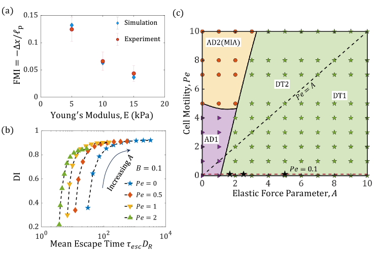
Figure 8: Comparison of cell migration index with experiment and a predicted durotactic phase diagram. (a) The forward migration index defined as the ratio of cell displacement towards the boundary and its total path length, FMI = $-{\Delta}x/l_{p}$, is calculated from simulations at $Pe=0.1$. Simulation results (blue diamonds) compare well with experimental data (orange circles) obtained by DuChez et al. for U-87 gliblastoma cells on a gradient of elastic substrate stiffness $2-18$ kPa.[23] The substrate had three different stiffness regions with effective Young’s modulus of $5$ kPa(soft), $10$ kPa(medium) and $15$ kPa (stiff). (b) Cells are more likely to show durotaxis if they have higher escape time. For given $Pe$ and $B$, increasing $A$ increases mean escape time, corresponding to Fig. (7), as well as DI. On the other hand, increasing $Pe$ reduces both mean escape time and DI. (c) We obtain a predicted phase diagram by classifying the simulation data points into three distinct regions. The durotactic region (green) corresponds to simulated cells (green pentagrams) with a durotactic index (DI, defined in Eq. (14)) greater than a threshold value DI$>0.4$, which corresponds to $A=1$ at $Pe=0$. The $Pe=A$ line separates the durotactic region into the diffusion-dominated regime (DT1) and motility-dominated regime (DT2). The cells outside the durotactic region (DI$<0.4$) are classified as adurotactic, AD1 (purple), or adurotactic with motility induced accumulation, AD2(MIA) (orange), depending on the accumulation of the cells at the boundary which is measured by accumulation index AI, defined in Eq. (48). Simulation points obtained for AD1 and AD2(MIA) regions are shown by triangles and circles respectively. Experimental data points observed by DuChez et al. ([23]) which are estimated to lie on the line $Pe=0.1$ are in the durotactic region (DT1) and represented by big pentagrams.

The elastic interaction parameter in our model, $A\sim P^{2}/E$, can be tuned by varying substrate stiffness, $E$. For a cell with fixed contractility $P$, the elastic interaction scales inversely with $E$, thus predicting a reduction in durotaxis with increasing substrate stiffness. We first compare our predictions with DuChez et al. [23], where the authors observed durotaxis of migrating U-87 glioblastoma cells up a stiffness gradient on polyacrylamide substrates. They quantified the extent of durotaxis as a forward migration index (FMI), defined as the ratio of the displacement of a cell up the stiffness gradient to its total path length. In our simulation setup, this corresponds to $-{\Delta}x/l_{p}$, that is, the ratio of displacement of the cell towards the clamped boundary to the total path length traversed along its trajectory. The substrate in the experiment comprised of three, connected, $250$ $\mu\mathrm{m}$-wide regions, labelled soft, medium, and stiff, with average Young’s moduli ($E$) of $5$ kPa, $10$ kPa and $15$ kPa, respectively. Thus, this work allows us to map the dependence of a tactic index on $A$ and $Pe$, thereby enabling direct comparison with our model predictions.

Using typical values for cell diameter, $\sigma\sim 20$ ${\mu}$m, and traction forces $\sim 2.5$ $nN$ [73], we estimate the elastic interaction parameter $A=B$ to be $5$, $2.5$, and $1.7$, corresponding to the three average substrate stiffness values in the experiment. We estimate $Pe\sim 0.1$ for cells in all these regions, based on their measured migration speed, $v_{0}\approx 0.4$ $\mu\mathrm{m}\mathrm{/}\mathrm{h}\mathrm{r}$,

and persistence time, $D_{R}^{-1}\approx 0.1$\mathrm{h}\mathrm{r}$$. The results from the simulation are plotted along with experimental data in Fig. 8(a). We find that the three data points for FMI from the experiment agree closely with those obtained from simulations for corresponding estimated $A=B$ values. Overall, this demonstrates that durotaxis increases when the cell is initially on softer substrates.

To classify our simulated results into qualitatively different regimes, we define tactic indices that predict the dependence of durotaxis on two key model parameters. These are $A$ (here we have chosen $B=A$) which represents the elastic cell-boundary interactions that drive durotaxis, and the persistent cell motility represented by $Pe$. Higher values of $Pe$ induce accumulation of cells at a confining boundary but also facilitate escape from “durotactic trapping” induced by the elastic potential. Thus, in our model setup, accumulation does not imply durotaxis. To distinguish accumulation from durotaxis, we separately define and calculate a durotactic index (DI) and an accumulation index (AI). We define these two quantities based on the steady state distribution of the simulated cells, specifically the previously defined $N_{\textrm{bound}}$, which represents the number of occurrences of a cell at the boundary. To define DI, we need to consider the accumulation driven by elastic interactions alone. We thus compare $N_{\textrm{bound}}$ at the same $Pe$ for $A\neq 0$ and $A=0$, and define DI as,

$$\mathrm{DI}=\frac{N_{\textrm{bound}}(A,Pe)-N_{\textrm{bound}}(A=0,Pe)}{N_{\textrm{bound}}(A,Pe)+N_{\textrm{bound}}(A=0,Pe)};$$ (14)

which allows us to subtract out the effect of motility-induced accumulation from the net accumulation. This may be visualized by considering a hypothetical simulation setup where say the left confining boundary has clamped elastic condition corresponding to $A\neq 0$, while the right confining boundary has no elastic interactions, $A=0$. This is represented in Fig. 13 in the Appendix, Section E. The difference in the number of accumulated cells on the left (expected to be more because of the elastic attraction) and the right at steady state is then our chosen measure of durotaxis. This is analogous to the definition of DI used in previous works [30, 28], where DI was taken to be the normalized difference in the number of steps $N_{f}$ in a cell trajectory in the “forward” direction - that is, the direction up a stiffness gradient, and the number of steps $N_{r}$ in the “reverse” (down the stiffness gradient) direction, $(N_{f}-N_{r})/(N_{f}+N_{r})$.

We observe that the DI metric clearly corresponds to the escape time trends as shown in (Fig. 7). We expect cells to be more durotactic when escape time is longer, which corresponds to higher $A$ and lower $Pe$. This is indeed borne out by the correlation between the values of DI and mean escape time ($\tau_{esc}$) measured in simulation, and shown in Fig. 8b. Each data point corresponds to the same values of $A$, $Pe$ and $B=0.1$. We thus show that the mean escape time from a confining boundary, which we can analytically calculate in the $Pe<A$ regime, is indeed a metric and predictor for the extent of durotaxis.

Next, we synthesize all simulation results for the clamped boundary case and organize them into a phase diagram. In the simulated $A-Pe$ phase diagram in Fig. 8c, we classify the region corresponding to DI above a critical value (DI $\geq 0.4$) to be “durotactic”. This choice corresponds to the calculated value of DI at $Pe=0$, $A=1$, since for $A\geq 1$ at $Pe=0$, we expect elastic attraction to dominate over diffusion (random cell motion). The phase boundaries are constructed by interpolating smoothly through 200 simulation data points ($A=0$ to $10$ and $Pe=0$ to $10$). The durotactic region can be further separated into two regimes by the line $Pe=A$. The $Pe<A$ region corresponds to a diffusion-dominated regime (DT1), where escape from the attractive boundary is facilitated by protrusion-facilitated random motion, corresponding to the analysis in Section D. The motility-dominated regime (DT2) occurs when $Pe>A$, and in this case escape from the attractive boundary is driven by persistent motility, without requiring any random translational motion, corresponding to the analysis in Section C. Thus, in each case, it is the random or persistent motility, given by $D$ and $Pe$ respectively, which primarily competes with elastic interactions to reduce durotaxis.

For $A<1$ or at high motility relative to elastic interactions $Pe\geq 5A$, the cells do not show sufficient durotaxis. These cells yield DI $<0.4$, and are not considered to be in the DT regime. They can still accumulate at the boundary if the motility is high enough. We denote this latter regime “motility induced accumulation” (AD2-MIA), and distinguish it from the adurotactic (AD1) region without accumulation, using an accumulation index (AI) defined in Eq. 48, in a complementary manner to the DI. The definition of AI is motivated by the form of the simulation setup used to define the DI, where the left (right) confining boundaries correspond to $A\neq 0$ and $A=0$ respectively, for a given $Pe$, (Appendix, Fig. 13). It extracts the amount of accumulation due to motility ($Pe$) alone by removing the effect of accumulation due to elastic interactions. At $A=0$, we consider the value of AI at $Pe=5$ to be the cut-off value (AI $=0.15$) to separate regions AD1 and AD2(MIA). AI $>0.15$ corresponds to MIA while AI $<0.15$ corresponds to AD1. All three datapoints from the DuChez et al. experiment [23] shown in Fig. 8a lie in the DI region of the phase diagram and are indicated by large stars Fig. 8b.

The main prediction of our simulation phase diagram is that durotaxis occurs when the strength of cell-boundary elastic interactions are large enough compared to random or persistent cell motility. This is realized when $A>A_{c}$, where the threshold value $A_{c}=1$ at $Pe=0$, and decreases with $Pe$. A higher $A$ can result from increased cell contractility, reduced substrate stiffness and less random cell movement. A higher persistent motility $Pe$ helps the cell escape the boundary interaction and reduces durotaxis. While the predicted dependence on substrate stiffness is borne out by the data from Ref. 23, the dependence on migration speed ($Pe$) is yet to be systematically tested in experiments, possibly because of the low value $Pe<1$ in many durotaxis experiments.

IV Discussion

In this work, we realize a statistical physical model for cell durotaxis by combining an elastic dipole model for an adherent cell with a phenomelogical model for persistent cell motility. We use this model to simulate cell dynamics during durotaxis at an elastic interface. The elastic dipole model for cell traction was invoked by Bischofs et al. [35, 36] to rationalize experimental observations of Lo et al. [17] that a fibroblast that is initially on the stiffer (softer) region, changes its orientation and aligns parallel (perpendicular) to the interface. The model as proposed was static and did not include the effect of cell motility (self-propulsion), which we now include. Our predictions for the reorientation (flipping) time given in Eq. (6), mean escape time from the attractive boundary in the presence of diffusion and self-propulsion, given by Eq. (13), and cell migration index values (Fig. 8) may be used to infer how durotaxis depends on cell traction force (via $A$, and $B$), substrate stiffness values (also via $A$ and $B$), and motility (via $Pe$). In this model setup, the accumulation of cells at the clamped (attractive) boundary facilitates durotaxis, since these cells can then cross over to the stiffer side. On the other hand, the motility-assisted escape from this boundary reduces durotaxis, since the cell can reorient and make its way back to the softer side.

Taken together, our theory and simulations indicate that the escape time $\tau_{\mathrm{esc}}$ depends on both cell-substrate elastic interaction and on motility, but in competing fashion. Consider a motile cell with $Pe>0$ that is initially oriented towards the stiffer side and at the interface. A “successful” durotaxis step would be the cell moving over to the stiffer side before it can reorient towards the softer side while at the interface, and migrate away. Our prediction that the escape time increases exponentially with the strength of cell-substrate elastic interaction, implies that the tendency for durotaxis increases as well. On the other hand, the cell’s motility enables its escape from the minimum of the elastic potential well arising from cell-substrate interactions and reduces the tendency to stay trapped at the attractive boundary. When diffusivity and elasticity parameters are held constant, our analysis predicts an exponential suppression of escape time with increasing $Pe$. Thus the extent of durotaxis may decrease substantially at larger values of the migration speed and persistence time. Our analysis of the escape time also suggests a dimensionless parameter that may be used to investigate cells moving up a smooth stiffness gradient. In the case of a gradient in the $x$ direction, a characteristic length scale $\lambda_{w}$ given by $\lambda^{-1}_{w}\sim E^{-1}(dE/dx)$ may be defined from the stiffness field $E(x)$. We interpret the continuous gradient as a series of potential wells, and use $\lambda_{w}$, as an estimate of the well width. Thus locally, a cell may be treated as undergoing persistent (durotactic) migration provided there is no significant reorientation and escape in the opposite direction as it is traversing this width. This happens provided $\lambda_{w}/v_{0}\ll D^{-1}_{R}\tau_{\mathrm{esc}}(E)$, suggesting that the dimensionless parameter $v_{0}D^{-1}_{R}\tau_{\mathrm{esc}}\lambda^{-1}_{w}$ may be a suitable metric to quantify the durotactic efficiency. A direct test of these predictions requires combined quantification of the cell migration trajectories and cell traction forces in the same experimental setup.

Based on our simulations, we predict a phase diagram of cell durotactic behavior. We show that durotaxis is enhanced when the cell-substrate elastic interactions are large enough, and the cell is not too motile. Our results quantitatively explain the finding by DuChez et al. [23] that the tactic index decreases with increasing local substrate stiffness. Our results are also qualitatively supported by the recent observation of Yeoman et al. [21] that weakly adherent breast cancer cells show comparatively less durotaxis than their strongly adherent counterparts. Weakly adherent cells are expected to undergo rapid assembly/disassembly of focal adhesions leading to faster motility as was indeed observed in the study. Faster cells are expected to have higher $Pe$ value according to an established universal exponential correlation between cell migration speed and persistence [74] based on experimental data. The observation that breast cancer cells are less durotactic is thus consistent with our predictions in Fig. 8(b). Yeoman et al. also performed traction force measurements and drug-treatment assays that inhibit the actomyosin cytoskeletal activity, but did not separately measure the effects of drug treatment on cell motility and contractility. Further experimental exploration using substrates of varying stiffness and adhesivity (e.g. by micropatterning) is needed to make quantitative and conclusive comparisons with our theoretical predictions for the dependence of escape time and durotactic index on cell traction and migration velocity. We also predict a motility-induced accumulation regime where cells are expected to be preferentially located near the confining boundary. While this has been demonstrated for active synthetic particles and swimming bacteria, this hitherto unexplored effect for crawling cells requires experiments on micropatterned substrates to confirm.

Recent observations of “negative durotaxis”, i.e., directed migration from softer to stiffer substrates suggest that cells do not always move up stiffness gradients, but rather move towards an optimal substrate stiffness where their contractility is maximal [26]. We note that the elastic dipole model can give rise to such an optimal stiffness when the mechanosensitivity of the cell to substrate properties is incorporated by including explicit feedback between cell traction force (the contractile dipole strength) and substrate deformation [29]. This is motivated by experiments that suggest that cells sense and adapt their traction and effective force dipole moment to substrate strain [75]. The inclusion of cell polarizability in the elastic dipole model creates additional interaction terms of the cell dipole with its image dipoles induced by the confining boundary. These additional pairwise interaction terms can be stronger and have the opposite sign from the direct interactions [76]. This may result in the clamped(free) boundary switching roles and being repulsive (attractive), which would drive negative durotaxis in our model. This effect will be explored in future work. In general, our work paves the way for exploring active cell migration under confinement and various tactic stimuli [77] that may be expressed as effective potentials.

Appendix

Appendix A Model for substrate mediated cell-interface interactions

Adherent cells exert dipolar contractile stresses on the underlying elastic substrate; these are generated by actomyosin fibers (actin and myosin II complexes), usually referred to as stress fibers, that generally connect the opposite sides of the cell and terminate at focal adhesions (FAs) [78, 13, 79]. On a larger scale, the entire contractile cell can be represented as a force dipole that deforms its extracellular environment typically modeled as a linear elastic continuum [13, 12]. The concept of force dipoles has found wide-ranging applications in various biological phenomena. [35, 36, 80, 81, 13, 82, 13, 29, 13, 83, 13].

Here, we use the force dipole concept and extend current theory to the interactions of active, motile cells with an underlying elastic substrate and constrained to remain within a domain (with boundaries) using a combination of simulations and analytical theory. In this minimal model, the entire, polarized cell, is coarse-grained and approximated as a single, evolving force dipole that moves on an elastic substrate, and is further subject to forces generated due to its interaction with the substrate and its boundaries. For the purposes of the analysis however, we use the word active to specifically mean self-propelling cells. Given the assumption of isotropic linear elasticity of the extracellular material, and the strength and orientation of the cell generated dipole, we can calculate stress and strain fields by solving the elastic equations with appropriate boundary conditions. These stress/strain fields then affect the motion of the cell by allowing cells to re-orient towards preferred alignments in order to optimize the deformation energy generated by the dipole in the substrate. Two canonical reference cases, namely 1) free boundaries, where the normal traction vanishes at the stiff-soft boundary (useful to analyze cells located on stiffer side), and 2) clamped boundaries, where the displacements vanish at the stiff-soft boundary (relevant to cells initially located on softer side) are analyzed. Such reduced descriptions are particularly appropriate when the stiffness contrast is high. The corresponding elastic boundary value problems with these limiting boundary conditions can be solved using the method of images [36].

In general, the interaction energy of the adherent cell (force dipole) with the surface [36] scales as $U\sim P^{2}f_{\nu}(\theta)/(Ex^{3})$, where $f_{\nu}$ is a function of substrate Poisson’s ratio $\nu$, and the orientation of the cell relative to boundaries. Here, the spatial and angular coordinates $x$ and $\theta$ are as defined in Fig. 11 -(c). The substrate mediated elastic cell-boundary interaction can be modeled as an effective potential $U(x,\theta)$ acting on the adherent cells (generating a force dipole) thus,

$$U(x,\theta) =-\left(\frac{P^{2}}{256\pi E}\right)\frac{f_{\nu}(\theta)}{\left(x+\sigma\right)^{3}},$$ (15)

$$f_{\nu}(\theta) =a_{\nu}+b_{\nu}\cos^{2}\theta+c_{\nu}\cos^{4}\theta,$$

with $P$ being the force dipole, $E$ and $\nu$ being the Young’s modulus and Poisson’s ratio of the substrate, respectively. The parameters $a_{\nu},b_{\nu},c_{\nu}$ are different for free and for clamped boundary conditions. These are, respectively (with superscript $f$ denoting free, and superscript $c$ denoting clamped)

$$a_{\nu}^{f} =-\frac{(1+v)[5+2v(6v-1)]}{(1-v)},$$ (16)

$$a_{\nu}^{c} =\frac{(1+v)[15+32v(v-1)]}{(1-v)(3-4v)}$$

$$b_{\nu}^{f} =-\frac{(1+v)[22+4v(2v-9)]}{(1-v)},$$

$$b_{\nu}^{c} =\frac{\left.(1+v)\left(34+32v^{2}-72v\right)\right]}{(1-v)(3-4v)}$$

$$c_{\nu}^{f} =-\frac{(1+v)\left[13(1-2v)+12v^{2}\right]}{(1-v)},$$

$$c_{\nu}^{c} =\frac{(1+v)(7-8v)}{(1-v)(3-4v)}$$

Preferred cell orientations, as predicted by calculating configurations that minimize deformation energy, are parallel/perpendicular to the boundary line for free/clamped boundaries. Hypothesizing that this holds even for motile cells, and accounting for the effects of self-propulsion, we deduce that motile cells preferentially move toward a clamped boundary, but tend to migrate away from a free boundary.

In addition to elastic effects, boundaries may physically constrain cells from crossing. This constraint is implemented by explicit displacements of the cells, as explained in the next section.

Table 1: List of biophysical parameters.

Parameter	Meaning	Value(s)
$\sigma$	Cell diameter	$10-100$   $\mu$m
$v_{0}$	Cell velocity	$0-80$   $\mu$m hr-1
$\mu_{T}$	Translational Mobility	0.1   m2 min-1 pN-1
$\mu_{R}$	Rotational Mobility	$25$  $\mu$m2 min-1
$D_{\mathrm{eff}}$	Rotational Diffusivity	$0.01-0.1$  min-1
$E$	Young’s modulus	$0.5-100$ kPa
$\nu$	Poisson’s ratio	$0.3$
$P$	Contractility	$10^{-12}-10^{-11}$ $\mathrm{N}\cdot\mathrm{m}$

Table 2: List of simulation parameters.

Parameter	Meaning	Definition	Value(s)
$A$	Cell-boundary force parameter	${\mu_{T}P^{2}\over(ED_{T}\sigma^{3})}$	$0.1-100$
$B$	Cell-boundary torque parameter	${\mu_{R}P^{2}\over(ED_{R}\sigma^{3})}$	$0.1-100$
$Pe$	Péclet Number	$v_{\mathrm{0}}\over\left(\sigma D_{\mathrm{R}}\right)$	$0-10$

Appendix B Simulation model details

The position and orientation of the cells is governed by over-damped Langevin equations. The simulation box has a square geometry with lateral dimension $L$ with $x$ representing the scaled distance measured normal to the boundary (see Fig. 1). We perform the simulations in dimensionless units. To do this, we choose $1/D_{R}$ as the characteristic time scale, and introduce dimensionless time $t^{*}$ related to dimensional time $t^{\prime}$ by $t^{*}\equiv t^{\prime}D_{R}$. The diameter of the cell $\sigma$ is used to scale lengths, so that the dimensionless positions $(x^{*},y^{*})$ are related to the dimensional ones $(x^{\prime},y^{\prime})$ via $x^{*}\equiv x^{\prime}/\sigma$, $y^{*}\equiv y^{\prime}/\sigma$ and ${\bf{r}}^{*}\equiv{\bf r}^{\prime}/\sigma$. The equations when scaled assume the form

$$\frac{d\mathbf{r}^{*}}{dt^{*}} = {Pe}\>\mathbf{p}\>-\frac{3A}{(x^{*}+1)^{4}}\tilde{f}_{\nu}(\theta)\hat{\mathbf{x}}+\sqrt{2D}{\bm{\eta}^{*}_{T}}$$ (17)

$$\frac{d\theta}{dt^{*}} = -\frac{B}{(x^{*}+1)^{3}}\frac{\partial\tilde{f}_{\nu}(\theta)}{\partial\theta}+\sqrt{2}\eta^{*}_{R}$$ (18)

where $A$ and $B$ are the dimensionless interaction parameters for force and torque respectively and $Pe$ is the Péclet number which determines the persistent motion of the cells( Eq. 4)). $D$ is the scaled coefficient of diffusion (Eq. (4)) while $\bm{\eta}_{T}^{*}$ and $\eta_{R}^{*}$ are the scaled Gaussian white noise for translation and rotation respectively. In our simulations $\nu$ is fixed at $0.3$ [17] and $f_{\nu}(\theta)$ is scaled such that $\tilde{f}_{\nu}(\theta)=(50/256\pi)f_{\nu}(\theta)$. Superscripts ^∗ in Eqs. (17) and (18) denote non-dimensional quantities. Henceforth, we will drop this superscript for ease of use and thus in the final equations simulated $(x,y,t)$ are all dimensionless.

Figure 9: The force from the boundary and active force orthogonal to the boundary both depend on the angle of orientation with the boundary. We compare the forces at the boundary to graphically estimate the angle of escape of the particles. We compare the force from the boundary (solid blue) at (a) $A=0.2$ and (b) $A=2$ with active forces perpendicular to the boundary (dashed) at $Pe=1,2,10$. The particle can escape at angles where the orthogonal component of the active force is greater than the boundary interaction. (a) At $A=0.2$, for all values of $Pe$, the particles can escape the boundary through any angle $\theta$ such that $cos{\theta}>0$. Increasing $Pe$ increases the angle of escape. (b) At $A=2$ we observe 3 different behaviors. For $Pe=1$ orthogonal component of active force is always less than the boundary force. At $Pe=10$, the active force is higher than the boundary force and intersect each other at 1 point. The active force is higher than the boundary force only inside angular pockets for $Pe=2$.

Appendix C Simulation methodology

Simulations are conducted, unless mentioned otherwise, with $N=200$ active Brownian particles (cells) of diameter $\sigma$. In scaled units, the cells have diameter of 1, and move within a square box of size $L=40$. Cells do not interact with each other. We choose the origin and coordinate axes $x$ and $y$ so that the domain is $-L/2\leq x\leq L/2$ and $-L/2\leq y\leq L/2$. Periodic boundary conditions are imposed at the lower and upper boundaries.

Lateral boundaries correspond to flat interfaces that interact elastically with cells and also impose confinement. We ignore deformations of the boundary so that these interfaces are always parallel to the y-axis at $x=-L/2$ and $x=L/2$. Confinement is directly imposed by maintaining an exclusion region of $\sigma/2$ exists around each interface; cells are thus prevented from partially or fully penetrating the wall. We implement this condition as follows. We make sure that if a particle makes a virtual displacement where the center of the particle is $x+\Delta x>L/2-\sigma/2$, it is brought back to a distance $L/2-\sigma/2$ and similarly to $-L/2+\sigma/2$ on the other confining boundary. The free and clamped boundary conditions are associated with the confining boundaries to ensure that the particles cannot cross the threshold potential. The coordinate system shown in Fig. 1-(c), demonstrates symmetry (in both the type of boundary conditions, and potential field from the boundary) about the origin $x=0$, and reflection symmetry about the $y$ axis. Since $x$ denotes the variable quantifying the normal distance measured from the edge of the boundary, our simulation methodology implies that particles are excluded from occupying a region of width $1/2$ (corresponding to the radius of the cell $\sigma/2$ in dimensional units) at the boundary (see Fig. 1-(c, f)).

Dimensionless forms of the dynamical equations Eq. 17-18 are discretized and numerically solved using the explicit half-order Euler-Maruyama method [84]. We initialize 200 non-interacting particles uniformly distributed inside the simulation box and study its probability distribution as function of distance from the boundary. These particles interact with the elastic boundaries depending on the proximity and orientation with respect to the boundary. Simulating a large number of non-interacting cells at the same time allows us to obtain detailed statistics for single particle interaction with the elastic boundary in a speedy and efficient manner. The dimensionless time step is $dt=10^{-3}$ such that the displacement in each time step is small ($\sim 10^{-2}\sigma$ or smaller). We sample the data every $10^{3}$ steps. When the probability distribution does not change with time (subject to a pre-specified precision), we consider that statistical steady state has been reached. Steady state is achieved at different times which depend on the parameters $A$, $B$ and $Pe$. Steady state time under no force or torque from the boundary can be estimated to be $\sim L^{2}/D_{\mathrm{eff}}$ where $D_{\mathrm{eff}}=v_{0}^{2}/D_{R}$. In our initial simulations, we set the scaled translational diffusion $D=0$. Thereafter, we study the distribution of particles as a function of distance from the boundary by averaging over all particles and time after steady state is achieved. We count the number of particles at $x=\sigma/2$ to determine the localization of particles at the boundary.

At steady state we look at the distribution of particles throughout the domain from the left wall to the midpoint of the domain, and also analyze the localization of particles near the boundary (over a region ranging from a cell diameter to a few cell diameters). This is done by studying the time evolution of the effective number of particles/cells a certain distance from the wall. If the interface was a penetrable surface, higher localization at the boundary would imply a higher probability of cells and a larger current/flux crossing the interface. For a free boundary, we study the effect of simulation parameters on the void length and orientation dynamics of particles at the clamped boundary. Our simulations complemented by a simple model for barrier crossing based on Kramer’s theories allow us to identify conditions particles can escape the influence of the boundary interactions.

Appendix D Determining escape conditions

Here we graphically explore the escape of particles from the boundary at different different interaction parameters, $A$, and Péclet number, $Pe$. We further determine the critical values $Pe_{1}(A)$ and $Pe_{2}(A)$ which dictate the different regimes of particle localization at the boundary. Particles remain trapped at the boundary when $Pe<Pe_{1}$. For $Pe>Pe_{2}$, there exists a characteristic angle $\theta$, above which trapped particles can attain a configuration favorable for escape from the boundary. This critical angle, $\theta_{\textrm{esc}}$ depends on $Pe$ (Fig. 5(a), Fig. 9(a)). For $Pe_{1}<Pe<Pe_{2}$ particles can only escape the boundary when their orientation $\theta$ lie in the angular region between $\theta_{1}$ and $\theta_{2}$ (Fig. 5(b)).

The particles can potential attain a configuration favorable for escape escape when the self-propulsion active force of the particle has an orthogonal component sufficient large to overcome the elastic attraction from the boundary. For a particle/cell trapped at the boundary $x=x_{b}=\sigma/2$, a balance yields

$$Pe={1\over\cos{\theta}}\>\frac{3A}{\left(x+1\right)^{4}}\tilde{f}_{\nu}(\theta),\quad\tilde{f}_{\nu}(\theta)=\frac{50}{256\pi}f_{\nu}(\theta).$$ (19)

At $Pe=Pe_{1}$, the tangent construction evaluating the elastic force originating due to cell-boundary interactions (see figure 9) provides $Pe_{1}$,

$$Pe_{1}=\frac{3A}{(x+1)^{4}}\frac{50}{256\pi}\left(2|b_{\nu}^{c}|\cos{\theta}+4|c_{\nu}^{c}|\cos^{3}{\theta}\right)$$ (20)

Eqs. (19) and (20) provide the ratio $Pe_{1}/A=0.91$ at $x=x_{b}=\frac{\sigma}{2}$. At $A=2$, $Pe_{1}=1.819$ and at $A=0.2$, $Pe_{1}$ is expected to be $0.182$.
To determine $Pe_{2}$, we consider $\theta_{1}=0$, since beyond $Pe_{2}$, $\theta_{1}$ would cease to exist as particles can escape at angles less than $\theta_{2}$. Balancing forces at $\theta=0$, we get

$$Pe_{2}=\frac{3A}{(x+1)^{4}}\frac{50}{256\pi}(|a_{\nu}^{c}|+|b_{\nu}^{c}|+|c_{\nu}^{c}|)$$ (21)

This gives the ratio $Pe_{2}/A=1.07$. For $A=2$, $Pe_{2}$ is determined to be $2.14$ and for $A=0.2$, it is $0.214$.

Appendix E Escape of cells from the attractive clamped boundary

E.1 Adaptation of Kramer’s theory to the frequency of orientation flips for spatially localized cells

Figure 10: (a) Schematic of the classical Kramers’ Problem for escape from a potential well and across a potential barrier. Particles move in a spatially varying potential $U(z)$, shown as the black curve, that is a function of a general coordinate $z$. The potential $U(z)$ exhibits two minima: the first at location $z=A$, and a second minimum beyond point $z=C$. Additionally, to get from $A$ to $C$, particles subject to $U(z)$ have to surmount and pass through a barrier with a local maximum at $z=B$ where $A<B<C$. We analyze an ensemble of particles initially in an equilibrium distribution at the bottom of the cell $z\sim A$, and study the rate at which they escape the barrier at $B$, and reach $C$. (b) Schematic of the barrier crossing problem for active self-propelled particle escaping from a potential well.

We analyze the flips in cell orientation, that is in the angle $\theta$, when the cell is at a fixed location near the boundary. This is done via an adaptation of the classical theory due to Kramer [70]. Consider a collection of independent Brownian cells/particles in an external 1D potential $U(z)$ that depends on a generalized coordinate $z$. Let the potential exhibit a meta-stable minimum at location $A$, with the maximum in the value occurring at the crest of a potential barrier at $B$, as shown in Fig. (10). The well is sufficiently deep so particles inside the well cannot escape in short time intervals. Assuming that particles in the well minima are close to equilibrium and cross the barrier diffusively, we aim to obtain the rate at which this escape takes place. The dynamics of a test particle can be described by the over-damped Langevin equation in 1D,

$$\frac{dz_{p}}{dt}=-\mu U^{\prime}(z_{p})+\eta(t)$$ (22)

with $\mu$ being the mobility and $-U^{\prime}(z_{p})$ the linear drag force acting on the particle located at $z_{p}$. The particle is also subject to a white noise $\eta(t)$, with zero mean $\langle\eta(t)\rangle=0$ and variance $\left\langle\eta(t)\eta\left(t^{\prime}\right)\right\rangle=2D\delta\left(t-t^{\prime}\right)$. Here $D$ and $\mu$ are generalized diffusivity and mobility coefficients that characterize the random diffusion and frictional effects as the particle/cell moves along $z$. Barrier crossing is achieved after many attempts - that is, the crossing is driven by diffusive processes.

These approximations allow us to move from the Langevin equation to the Fokker-Planck equivalent. We recast the problem in terms of a probability distribution function $P(z,t)$ that may be mapped to either the probability of a single particle or the density of a collection of particles (as in simulations). We assume that the system is close to equilibrium so that crossing flux $J(z,t)$ may be related to gradients in $P(z,t)$,

$$\frac{\partial P(z,t)}{\partial t} = \frac{\partial}{\partial z}\left[\mu\frac{\partial U}{\partial z}P+D\frac{\partial P}{\partial z}\right]=-\frac{\partial J}{\partial z}$$ (23)

$$J = -\mu P(z,t)\partial_{z}U-D\partial_{z}P(z,t)$$ (24)

$$J = -De^{-\frac{U(z)}{k_{B}T}}\frac{\partial}{\partial z}\left(e^{\frac{U(z)}{k_{B}T}}P(z)\right).$$ (25)

We have invoked the Stokes-Einstein relationship so that $D=\mu k_{B}T$. For a system that is approximately in equilibrium and in quasi-steady conditions with a large barrier height satisfying $[U(B)-U(A)]/(k_{B}T)\ll 1$, the current $J$ across the barrier is small and the rate of depletion at the well is small. Since the system is close to quasi-steady sate, the probability distribution $P(z,t)$ doesn’t change quickly with time, and so $\partial_{t}P(z,t)\approx 0$. Moreover, based on Eq. 23, the current is then to leading order constant and independent of $z$ and $t$.

$$\frac{J}{D}e^{\frac{U(z)}{k_{B}T}}=-\frac{\partial}{\partial z}\left[e^{\frac{U(z)}{k_{B}T}}P(z,t)\right].$$ (26)

Due to the barrier crossing event being a rare event, we next invoke the approximation $P(A)\gg P(C)\sim 0$.

To calculate the escape flux, we assume that re-crossings into the well are not permitted once the particle reaches location $C$. That is, we let $C$ correspond to an absorbing boundary so that the probability density there is zero. Integrating Eq. 26 between locations $A$ and $C$, and using $P(C)=0$, we obtain

$$\frac{J}{D}{\int_{A}^{C}e^{\frac{U\left(z\right)}{k_{B}T}}dz}=e^{\frac{U(A)}{k_{B}T}}P(A).$$ (27)

The left side integral can be asymptotically estimated to leading order by using the saddle point method by expanding $U(z)$ in a Taylor series approximation and noting that the first derivative at $B$ is zero,

$$\int_{A}^{C}e^{\frac{U\left(z\right)}{k_{B}T}}dz\approx\int_{A}^{C}e^{\frac{U(B)+\frac{1}{2}U^{\prime\prime}(B)\left(z-B\right)^{2}}{k_{B}T}}dz$$ (28)

$$\approx e^{\frac{U(B)}{k_{B}T}}\int_{-\infty}^{\infty}e^{\frac{-\left|U^{\prime\prime}(B)\right|\left(z-B\right)^{2}}{2k_{B}T}}dz=e^{\frac{U(B)}{k_{B}T}}\sqrt{\frac{2\pi k_{B}T}{\left|U^{\prime\prime}(B)\right|}}.$$

To evaluate the escape rate $r_{\mathrm{esc}}$, we recognize that this rate is the same as the current going out of the metastable well at $A$, given that the particles are initially situated inside it, $J=p_{A}r_{\mathrm{esc}}$. Assuming an initial close equilibrium state with

$$P(z)=P(A)\exp\left[-[U(z)-U(A)]/k_{B}T\right]$$

and using the expansion

$$U(z)\approx U(A)+\frac{1}{2}U^{\prime\prime}(A)(z-A)^{2},$$

the probability to be inside the well is approximately

$$p_{A}=\int_{A-\Delta}^{A+\Delta}P(z)\>dz \approx P(A)\int_{-\infty}^{\infty}e^{-\frac{U^{\prime\prime}(A)\left(z-A\right)^{2}}{2k_{B}T}}dz$$ (29)

$$=P(A)\sqrt{\frac{2\pi k_{B}T}{U^{\prime\prime}(A)}}.$$

Here $\Delta$ denotes a suitably small range in the neighborhood of point A. The saddle point approximation allows us to eventually extend the domain of integration from $-\infty$ to $\infty$. Thus, the escape time satisfies,

$$\tau_{\mathrm{esc}}={1\over r_{\mathrm{esc}}}=\frac{p_{A}}{J}={{2\pi k_{B}T\exp{\left(\frac{U(B)-U(A)}{k_{B}T}\right)}}\over{D{\sqrt{U^{\prime\prime}(A)\left|U^{\prime\prime}(B)\right|}}}}$$ (30)

To use Eq. 30 to study flipping dynamics, we consider a particle located at a fixed position $x$ and study the time it takes to reorient from $\theta=0$ (bottom of the potential well), to $\theta=\pi/2$ (top of the barrier). The escape time can be mapping into the $1D$ circle motion with periodic boundary condition $P(\theta=0)=P(\theta=2\pi)$ (cite Sommerfeld’s book). Identifying the coordinate $z$ as $\theta$ and reintroducing the location dependence $x$ (here considered constant), we obtain the escape time at fixed $x$

$$\tau_{\mathrm{esc}}D_{R} =\frac{2\pi k_{B}T\exp\left(\frac{U(x,\pi/2)-U(x,0)}{k_{B}T}\right)}{\sqrt{\left[U^{\prime\prime}(x,0)\left|U^{\prime\prime}(x,\pi/2)\right|\right]}}$$ (31)

$$\sim\frac{1}{B}\exp\left(\frac{B}{B^{*}}\right).$$

Figure 11: (a) The mean escape time evaluated from simulation (solid black circles) follows the modified Kramer’s theory of barrier crossing for passive particles with $Pe=0$ moving in the 1D modified potential without the coupling between position and orientation ($\tilde{f}=1$). In the limiting cases resulting in Eq. 39, the solid line and dashed line represent the analytical results and the approximation, respectively. (b) Results for the mean escape time from simulations (black circle, red square and blue star symbols) for passive particles in 1D, and with $B=2,0.1$ in 2D, respectively. Values of effective $f^{*}$ averaged over orientational degrees of freedom is by fitting and estimated to be $0.788$ and $0.651$ for $B=2,0.1$, respectively. For larger $B$, the particles always flip between orientations $\theta=0$ and $\theta=\pi$, and thus confirm to the 1D situation. Thus, the upper bound of $f^{*}$ is given by $1$ corresponding to 1D case. The lower bound could be estimated by the $f^{*}\approx\tilde{f}(\theta=\pi/2)$.

E.2 1D and 2D passive case: Escape time without self-propulsion in attractive power-law potentials

Here we focus on a motile test cell $Pe>0$ that is in the attractive domain. As discussed earlier, the wall induced elastic potential $U(x,\theta)$ depends on both cell distance normal to the boundary $x$, and cell orientation $\theta$. To understand the escape for motile cells, we first investigate escape dynamics for non-motile cells and set $Pe=0$. This result will form the foundation for our analysis of activity assisted escape that is valid for small values of $Pe$.

Let us first consider possibly the simplest case - the dynamics of a non-motile cell/particle in one dimension. Specifically, we assume there is no orientation coupling $f_{\nu}(\theta)=1$ and so the potential $U$ is a function of $x$ alone. The physical motivation for this comes from the recognition that $U(x,\theta)$ is the product of two functions one of which depends only on $x$, and the second (via $f_{\nu}(\theta)$) depends on $\theta$ alone. When cell reorientations occur on time-scales that are much shorter than the time for cells to escape, it is possible to average over accessible orientations and replace the function $f$ with a suitably averaged constant (which for our simulations with fixed $D$ and $D_{R}$ is a pure number). Biologically, such a process is applicable to cells with rapid and highly stochastic blebbing.

Since there is no saddle point in the original potential derived from elastic interactions (a power-law potential), we consider a modified potential $U(z)$ (in $k_{B}T$ units) with $z$ being a (scaled) coordinate obtained by replacing the term $(z+1)^{-3}$ with $(z^{2}+1)^{-3/2}$ so that

$$U(z)=-{A\over(z^{2}+1)^{3/2}},\>\>\>{\mathrm{with}}\>\>\>A\equiv\left({{P^{2}\langle f_{\nu}\rangle}\over{256\pi Ek_{B}T}}\right).$$ (32)

The Fokker-Planck equation for the probability ${\Psi}$ in terms of $z$ and (scaled) time $\tau$ may then be written

$$\frac{\partial\Psi}{\partial\tau} = \frac{\partial}{\partial z}\left(\frac{\partial\Psi}{\partial z}+\Psi\frac{\mathrm{d}U}{\mathrm{~{}d}z}\right)$$ (33)

We use the method of separation of variables to convert Eq. 33 into an eigenvalue problem. Setting $\Psi(z,\tau)=\mathrm{e}^{-U(z)}g(z)\mathrm{e}^{-\mu\tau}$ where $g(z)$ then quantifies a small deviation from the equilibrium solution as $\tau\rightarrow\infty$, we find

$$\frac{\mathrm{d}^{2}g}{\mathrm{~{}d}z^{2}}-\frac{\mathrm{d}U}{\mathrm{~{}d}z}\frac{\mathrm{d}g}{\mathrm{~{}d}z}+\mu g=0.$$ (34)

The appropriate boundary conditions may be deduced from the simulations. At the local minimum $z^{*}=z=0$, we assume an impenetrable boundary that prevents particles from escaping, and so $g^{\prime}(0)=0$. Meanwhile, we can define the annihilation point being $z=L_{\rm esc}$ where the potential is indeed nearly flat at this point.

Now, if the potential well is sufficiently deep, the method of dominant balance can be used to show that the behavior of $g(z)$ is largely determined by the asymptotic behavior of $U(z)$ for $z\gg 1$. We denote this long-range attraction by $U(z)=-Az^{3}$, and exploit the fact that $\mu$ is exponentially small. Thus we may write

$$\frac{\mathrm{d}^{2}g}{\mathrm{~{}d}z^{2}}-\frac{\mathrm{d}U}{\mathrm{~{}d}z}\frac{\mathrm{d}g}{\mathrm{~{}d}z}=0$$ (35)

and therefore,

$$g(z)=\int_{z}^{L_{\rm esc}}e^{U(z^{\prime})}dz^{\prime}.$$ (36)

Since $g(z)$ was computed under the assumption that $\mu\simeq 0$, it represents a pseudo-steady solution. Applying this to the corresponding Kramers formulation for the escape flux, which gives the rate constant as the ratio of the steady-state flux to the number of reactant particles, and using $g(L_{\rm esc})$ = 0, we get

$$\mu =\frac{g\left(z^{*}\right)-g(L_{\rm esc})}{\int_{z^{*}}^{L_{\rm esc}}\mathrm{e}^{U(z^{\prime})}\mathrm{d}z^{\prime}\int_{0}^{L_{\rm esc}}\mathrm{e}^{-U(z^{\prime})}g(z^{\prime})\mathrm{d}z^{\prime}}$$ (37)

$$=\left[\int_{0}^{L_{\rm esc}}\mathrm{e}^{U(z)}\mathrm{d}z\int_{0}^{L_{\rm esc}}\mathrm{e}^{-U(z)}\mathrm{d}z\right]^{-1}.$$

We estimate the integrals as follows:

$$\int_{0}^{L_{\rm esc}}\mathrm{e}^{U(z)}\mathrm{d}z =\frac{{L_{\rm esc}}}{3}\left(\frac{A}{L_{\rm esc}^{3}}\right)^{\frac{1}{3}}\Gamma\left[-\frac{1}{3},\frac{A}{{L_{\rm esc}^{3}}}\right]$$ (38)

$$\stackrel{{\scriptstyle\frac{A}{L_{\rm esc}^{3}}\ll 1}}{{\longrightarrow}}{L_{\rm esc}}+\frac{1}{3}\Gamma[-\frac{1}{3}]A^{\frac{1}{3}}$$

$$\int_{0}^{L_{\rm esc}}\mathrm{e}^{-U(z)}\mathrm{d}z \sim\frac{1}{\sqrt{A}}\mathrm{e}^{A}$$

where we retained only the leading order asymptotic terms in the expansion leading to Eq. 38. Note that our simulation parameters are $L_{\rm esc}=6$, with $1<A<12$, and hence ${L_{\rm esc}}>A^{1/3}$ as required for this approximation to hold. The specific parameter evaluates to $\Gamma[-1/3]/3=-1.35$, which we approximate to obtain an asymptotic estimate for the escape time,

$$\tau_{\mathrm{esc}}\approx(L_{\rm esc}+\frac{1}{3}\Gamma[-\frac{1}{3}]A^{\frac{1}{3}})\frac{1}{\sqrt{A}}\mathrm{e}^{A}\approx\frac{(L_{\rm esc}-A^{\frac{1}{3}})}{\sqrt{A}}\mathrm{e}^{A}$$ (39)

In the 1D passive case considered here, there is no rotational diffusion $D_{R}$, and the characteristic relaxation time $\sigma^{2}/D_{T}$ is used to convert dimensional times to dimensionless ones.

The form of Eq. 39 motivates an extension of the results to the escape of a particle subject to a more complex orientation and space dependent 2D potential $U(z,\theta)$. We still assume a passive particle so that $\mathrm{Pe}=0$. The physical boundary is such that the test cell particle is on the soft side. Since orientational effects are to be considered here, we expect that the escape time will now depend on both $A$ and $B$ rather than on $A$ alone. Based on these observations, propose the ansatz

$${\tau_{\mathrm{esc}}}=\left({1\over D_{R}}\right)\>m(B)\left(\frac{L_{\rm esc}-A^{1\over 3}}{\sqrt{A}}\right)\exp{\left[Af^{*}(B)\right]}.$$ (40)

Here $f^{*}(B)$ is an effective parameter which comes from the coupling between the positional and orientational coupling. Parameter $m(B)$ takes into account the two dimensional nature of the potential and explicitly corrects for orientational effects on possible escape trajectories, and thus escape time.

It is useful to briefly consider the $(L_{\rm esc}-A^{1\over 3})$ term in Eq. 40. Escape from the potential well is dominated by two effects depending on the distance from the well minimum. Close to the minimum, the potential dominates and the particle moves with an effective speed that depends on the force due to the potential. At distances $\sim A^{1\over 3}$, the strength of the potential is unity, and thus for distances larger than this value, diffusion dominates and aides the escape over the barrier. One may treat $(L_{\rm esc}-A^{1\over 3})$ as an effective distance over which particles diffuse in order to leave the well.

Figure 12: (a) The fitting pre-factor $m(Pe)$ (black squares) follows a linear form $m(Pe)=4.24-1.74\>Pe$ (dashed line) for $B=0.1$. (b) For $f^{*}=1$, the magnitude (extent) of the $\Delta C$ region increases as $A$ increase, but decreases as $Pe$ increases.

E.3 Activity-assisted escape from the attractive clamped boundary for small and $O(1)$ $Pe$: Reduced durotaxis

We conclude by analyzing the escape dynamics of migratory, motile cells from clamped boundaries. In our simplified model, they correspond to active motile particles with $Pe>0$ moving in a suitable 2D potential with orientational coupling.

Even for the 2D passive case, the substrate-mediated cell-boundary potential $U(x,\theta)$ with full coupling between position $r$ and orientation $\theta$ it is difficult to exactly calculate the escape time. To make the theory tractable while still remaining faithful to the physics of the problem, we introduced a parameters $f^{*}$ to quantify the effective coupling effects as in Eq. 40. Since the orientation dynamics are highly dependent on parameter $B$, we further assumed $f^{*}$ is determined by $B$. Using this approximate treatment, the escape time problem can be reduced to barrier crossing of run and tumble particles (or diffusing particles) in a 1D trap.

Recently, it was shown for a run-and-tumble active particles that the escape time from a trap depends on the detailed structure of the potential [72]. Importantly, it is not a simply exponential function of the potential depth as shown in the classical Kramer’s theory. Woillez et al [72] recently investigated the activated escape of run-and-tumble particles from metastable wells, an example of which is illustrated in Fig. 10 (b). In the figure, $C_{1},C_{2}$ are locations satisfying $\partial_{z}U(C_{i})=v_{0}/\mu_{T}$ where the potential force arising from the elastic interaction equals the self-propulsion force. The minimal action for the particle to escape from the potential well is to move right away from the base of the well (with orientation angle, $\theta=0$). The most probable path is then given by

$$\mathcal{A}[z]=\frac{1}{4}\int_{\infty}^{\infty}(\dot{z}+\mu_{T}\partial_{z}U(z)-v_{0})^{2}dt^{\prime}$$ (41)

Following the arguments in Woillez et al [72], we find the instanton solution obeys $\dot{z}=\partial_{z}\{\mu_{T}[U(z)-U(C_{1})]-v_{0}(z-C_{1})\}\equiv\partial_{z}\varphi(z)$. The problem with self-propulsion may then be analyzed in an equilibrium setting with an effective tilted potential $\varphi(z)/\mu_{T}$ that is modified by the activity. Thus the escape time from the trap depends exponentially on the modified potential barrier as $\langle\tau_{\mathrm{esc}}\rangle\propto\exp(\phi/D_{T})$ in the limit of $D_{T}\to 0$. The quasi-potential barrier is $\phi=\mu_{T}[U(z)-U(C_{1})]-v_{0}(z-C_{1})$, after modification by the self-propulsion speed $v_{0}$.

In our case, the escape dynamics for the 2D passive particles from the barrier (the annihilation point $L$) in the 1D power-law like potential $U(x)/k_{B}T=-{Af^{*}/(x^{2}+1)^{3/2}}$, can be reduced to barrier crossing of diffusing particles in a 1D trap by introducing an effective parameter $f^{*}$. Then, the escape dynamics in the 2D active particles simplify to the escape problem of run-and-tumble particles in the power-law-like potential as in Woillez et al [72]. We assume the pre-factor depending on the dimensionless parameters $A$ in the active case is the same as the passive case. The mean escape time of particles crossing the barrier can be written as

$$\tau_{\mathrm{esc}}=\left(\frac{L_{\rm esc}-A^{1\over 3}}{\sqrt{A}}\right)m(B,Pe)\exp\left(\frac{\phi\left(v_{\mathrm{0}}\right)}{D_{T}}\right)$$ (42)

$$\phi(v_{0})=\mu_{T}\left[U\left(C_{2}\right)-U\left(C_{1}\right)\right]-v_{\mathrm{0}}\left(C_{2}-C_{1}\right).$$ (43)

where the effective dimensional potential $\phi(v_{0})$ involves the effects of active work due to the self-propulsion speed $v_{0}>0$ ($Pe>0$). Note that for the passive case, $v_{0}=0$ and therefore $Pe=0$. Coordinate values (points) $C_{2},C_{1}$ that are spatial locations are functions of ${\mathrm{Pe}}$ and $A$ where the active self-propulsion force balances the elastically derived interaction force. In dimensional form, these locations satisfy the conditions

$${v_{\mathrm{0}}\over\mu_{T}}=|\partial_{x}U(x,\theta)|,\>\>\>{\mathrm{at}}\>\>\>x=C_{1},\>x=C_{2}.$$ (44)

For the passive case $v_{0}=0$ and so $Pe=0$, and we find $C_{1}=0$ and $C_{2}\sim L$ (that is $L_{\mathrm{esc}}$ in simulation terminology). For the active motile case where $Pe>0$, the dimensional balance when scaled yields,

$$\frac{\left(\tilde{x}^{2}+1\right)^{\frac{5}{2}}}{\tilde{x}}|_{\tilde{C_{2}},\tilde{C_{1}}}=\frac{3Af^{*}}{Pe},$$ (45)

Note that the two points $\tilde{C}_{i}=C_{i}/\sigma$ depend on dimensionless parameters $A,B$ and $\mathrm{Pe}$. The form of the quasi-potential barrier is as follows,

$$\frac{\phi}{D_{T}}=\frac{Af^{*}}{(\tilde{C_{1}}^{2}+1)^{3\over 2}}-\frac{Af^{*}}{(\tilde{C_{2}}^{2}+1)^{3\over 2}}-Pe\left(\tilde{C_{2}}-\tilde{C_{1}}\right).$$ (46)

Further imposing that $f^{*}$ depend only the parameter $B$ (in the limit of small $Pe$), we replace $f^{*}$ by the corresponding values for the 2D $Pe=0$ passive case at the same $B$. The pre-factor function $m(B,Pe)$ however remains dependent on both $B$ and on $Pe$. In order for the $Pe\rightarrow 0$ limit of this theory to yield the 2D escape time estimate calculated earlier, we require $m(B,Pe)$ to be a linear function of $Pe$. Combining these ideas, we propose that

$$\tau_{\mathrm{esc}}=\left(\frac{L_{\rm esc}-A^{1\over 3}}{\sqrt{A}}\right)\>m(B,\mathrm{Pe})\exp(\frac{\phi}{D_{T}})$$ (47)

At $B=0.1$, $f^{*}=0.651$. The fitting pre-factor $m$ is found to be $m(Pe)=4.24-1.74\>Pe$ as shown in Fig. 12-(a). Furthermore, $\Delta C(Af^{*},Pe)\equiv\tilde{C_{2}}-\tilde{C_{1}}$ depends strongly on $A$ and $Pe$ as shown in Fig. 12 (b).

Appendix F Measurement of tactic indices from simulation

Figure 13: To calculate DI (Eq. 14) and AI (Eq. 48) we simulate and combine results of four cases – $(A\neq 0,Pe\neq 0)$, $(A=0,Pe\neq 0)$, $(A\neq 0,Pe=0)$, and $(A=0,Pe=0)$ as illustrated here. For the $A\neq 0$ cases, we simulate a clamped impenetrable boundary and an elastic substrate on which cells move towards or away from the boundary. For $A=0$, we simulate an impenetrable boundary and a non-elastic substrate on which cells move. To calculate DI, we compute the accumulation of cells at each boundary – specifically $N_{\mathrm{bound}}(A\neq 0)$ and $N_{\mathrm{bound}}(A=0)$. We define AI by accounting for the the increased boundary accumulation due to cell motility ($Pe>0$) via (Eq. 48).

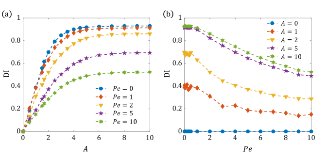
Figure 14: The durotactic index DI as defined in Eq. 14 is plotted here in two ways. In (a), we observe that DI increases with elastic force parameter, $A$ when $Pe$ is held constant and reaches limiting values. (b) For $A$ held fixed, we find that DI decreases with cell motility, $Pe$. The index is $0$ by definition for $A=0$.

Here we summarize the methodology used to compute the various tactic indices used in the main text, from our simulations. One of these metrics, the FMI is used to compare our results with the analysis of experiments in Ref. 23. In these experiments, cells were tracked every 15 minutes and the FMI was calculated at $1$ hour intervals, for a total period of $24$ hours. The authors also quantified the persistence of trajectories by estimating the ratio of displacement and the distance covered by the cell in these $1$ hour intervals. This quantity was measured to be approximately $0.35$ for cells moving in all three regions. The persistence time – that is, the time over which the cells travel more-or-less in the same direction – is around $0.1$ hour. To calculate the FMI defined in Ref. 23 from our simulations, the following procedure was used. The position of a test cell is tracked every ${\Delta}T=2.5$ dimensionless times ($15$ minutes in experiments). From these positions, the FMI is evaluated every ${\Delta}T=10$ times ($1$ hour in experiments). Cells move in the domain and sometimes upon reaching the boundary travel long its side. We do not consider the contribution of particles trapped at the boundary or traveling along the boundary in the FMI calculation, since the biological experiments are in unconfined geometries (corresponding to cells at the boundary just crossing over). We also only evaluated the FMI for up to a dimensionless observation time $T=10$ since most particles reach the boundary within that time. We calculate FMI inside a region $6\sigma$ from the boundary since we already established that beyond this region the influence from the boundary elastic potential is very low.

To calculate durotactic index (DI) and accumulation index (AI), we combine the results of two different simulations, $A\neq 0$ and $A=0$, corresponding to the same value of $Pe$. Here $A$ ranges from $0-10$. In these simulations we consider the same elastic force and torque interaction parameters for cells with the boundary such that $A=B$. Then, we consider the difference in the steady state numbers of cells localized at the boundary between $A\neq 0$ and $A=0$, to calculate the DI. We observe that DI increases with $A$ and reaches a limiting va$A\neq 0$ and $A=0$.lue at all values of $Pe$ (Fig. 14(a)), while for given $A$, the DI decreases with $Pe$ (Fig. 14(b)). The accumulation index (AI) used in the main text is defined as:

$$\mathrm{AI}=\frac{N_{\mathrm{bound}}(A,Pe)+N_{\mathrm{bound}}(A=0,Pe)-(N_{\mathrm{bound}}(A,Pe=0)+N_{\mathrm{bound}}(A=0,Pe=0))}{N_{\mathrm{total}}(A,Pe)+N_{\mathrm{total}}(A=0,Pe)}$$ (48)

which is motivated by the form of the simulation setup used to define the DI, shown in Fig. 13. Here, the left (right) confining boundaries correspond to $A\neq 0$ and $A=0$ respectively, for a given $Pe$. This choice of AI allows us to subtract out the effect of accumulation due to $A$ only, from from the net accumulation. We thus obtain the amount of accumulation due to motility ($Pe$) alone.

References

- Yamada and Sixt [2019] K. M. Yamada and M. Sixt, Mechanisms of 3d cell migration, Nature Reviews molecular cell biology 20, 738 (2019).
- Bechinger et al. [2016] C. Bechinger, R. Di Leonardo, H. Löwen, C. Reichhardt, G. Volpe, and G. Volpe, Active particles in complex and crowded environments, Reviews of Modern Physics 88, 045006 (2016).
- Romanczuk et al. [2012] P. Romanczuk, M. Bär, W. Ebeling, B. Lindner, and L. Schimansky-Geier, Active brownian particles, The European Physical Journal Special Topics 202, 1 (2012).
- Redner et al. [2013] G. S. Redner, M. F. Hagan, and A. Baskaran, Structure and dynamics of a phase-separating active colloidal fluid, Biophysical Journal 104, 640a (2013).
- Cates and Tailleur [2015] M. E. Cates and J. Tailleur, Motility-induced phase separation, Annual Review of Condensed Matter Physics 6, 219 (2015).
- SenGupta et al. [2021] S. SenGupta, C. A. Parent, and J. E. Bear, The principles of directed cell migration, Nature Reviews Molecular Cell Biology 22, 529 (2021).
- Alberts [2017] B. Alberts, Molecular biology of the cell (Garland science, 2017).
- Friedl et al. [2011] P. Friedl, K. Wolf, and J. Lammerding, Nuclear mechanics during cell migration, Current opinion in cell biology 23, 55 (2011).
- Selmeczi et al. [2005] D. Selmeczi, S. Mosler, P. H. Hagedorn, N. B. Larsen, and H. Flyvbjerg, Cell motility as persistent random motion: theories from experiments, Biophysical journal 89, 912 (2005).
- Gardel et al. [2010] M. L. Gardel, I. C. Schneider, Y. Aratyn-Schaus, and C. M. Waterman, Mechanical integration of actin and adhesion dynamics in cell migration, Annual Review of Cell and Developmental Biology 26, 315 (2010), pMID: 19575647.
- Pelham and Wang [1997] R. J. Pelham and Y.-l. Wang, Cell locomotion and focal adhesions are regulated by substrate flexibility, Proceedings of the National Academy of Sciences 94, 13661 (1997).
- Balaban et al. [2001] N. Q. Balaban, U. S. Schwarz, D. Riveline, P. Goichberg, G. Tzur, I. Sabanay, D. Mahalu, S. Safran, A. Bershadsky, L. Addadi, et al., Force and focal adhesion assembly: a close relationship studied using elastic micropatterned substrates, Nature cell biology 3, 466 (2001).
- Schwarz and Safran [2013] U. S. Schwarz and S. A. Safran, Physics of adherent cells, Rev. Mod. Phys. 85, 1327 (2013).
- Chaudhuri et al. [2020] O. Chaudhuri, J. Cooper-White, P. A. Janmey, D. J. Mooney, and V. B. Shenoy, Effects of extracellular matrix viscoelasticity on cellular behaviour, Nature 584, 535 (2020).
- Angelini et al. [2010] T. E. Angelini, E. Hannezo, X. Trepat, J. J. Fredberg, and D. A. Weitz, Cell migration driven by cooperative substrate deformation patterns, Phys. Rev. Lett. 104, 168104 (2010).
- Notbohm et al. [2016] J. Notbohm, S. Banerjee, K. J. Utuje, B. Gweon, H. Jang, Y. Park, J. Shin, J. P. Butler, J. J. Fredberg, and M. C. Marchetti, Cellular contraction and polarization drive collective cellular motion, Biophysical journal 110, 2729 (2016).
- Lo et al. [2000] C.-M. Lo, H.-B. Wang, M. Dembo, and Y.-l. Wang, Cell movement is guided by the rigidity of the substrate, Biophysical journal 79, 144 (2000).
- Shellard and Mayor [2021a] A. Shellard and R. Mayor, Durotaxis: the hard path from in vitro to in vivo, Developmental cell 56, 227 (2021a).
- Sunyer and Trepat [2020] R. Sunyer and X. Trepat, Durotaxis, Current Biology 30, R383 (2020).
- Raab et al. [2012] M. Raab, J. Swift, P. D. P. Dingal, P. Shah, J.-W. Shin, and D. E. Discher, Crawling from soft to stiff matrix polarizes the cytoskeleton and phosphoregulates myosin-ii heavy chain, Journal of Cell Biology 199, 669 (2012).
- Yeoman et al. [2021] B. Yeoman, G. Shatkin, P. Beri, A. Banisadr, P. Katira, and A. J. Engler, Adhesion strength and contractility enable metastatic cells to become adurotactic, Cell reports 34, 108816 (2021).
- Park et al. [2016] J. Park, D.-H. Kim, H.-N. Kim, C. J. Wang, M. K. Kwak, E. Hur, K.-Y. Suh, S. S. An, and A. Levchenko, Directed migration of cancer cells guided by the graded texture of the underlying matrix, Nat. Mater. 15, 792 (2016).
- DuChez et al. [2019] B. J. DuChez, A. D. Doyle, E. K. Dimitriadis, and K. M. Yamada, Durotaxis by human cancer cells, Biophysical journal 116, 670 (2019).
- Sunyer et al. [2016] R. Sunyer, V. Conte, J. Escribano, A. Elosegui-Artola, A. Labernadie, L. Valon, D. Navajas, J. M. García-Aznar, J. J. Muñoz, P. Roca-Cusachs, et al., Collective cell durotaxis emerges from long-range intercellular force transmission, Science 353, 1157 (2016).
- Shellard and Mayor [2021b] A. Shellard and R. Mayor, Collective durotaxis along a self-generated stiffness gradient in vivo, Nature 600, 690 (2021b).
- Isomursu et al. [2022] A. Isomursu, K.-Y. Park, J. Hou, B. Cheng, M. Mathieu, G. A. Shamsan, B. Fuller, J. Kasim, M. M. Mahmoodi, T. J. Lu, et al., Directed cell migration towards softer environments, Nature materials 21, 1081 (2022).
- Hartman et al. [2016] C. D. Hartman, B. C. Isenberg, S. G. Chua, and J. Y. Wong, Vascular smooth muscle cell durotaxis depends on extracellular matrix composition, Proc. Natl. Acad. Sci. 113, 11190 (2016).
- Yu et al. [2017] G. Yu, J. Feng, H. Man, and H. Levine, Phenomenological modeling of durotaxis, Physical Review E 96, 010402 (2017).
- Zemel et al. [2010] A. Zemel, F. Rehfeldt, A. E. X. Brown, D. E. Discher, and S. A. Safran, Optimal matrix rigidity for stress-fibre polarization in stem cells, Nature Physics 6, 468 (2010).
- Novikova et al. [2017] E. A. Novikova, M. Raab, D. E. Discher, and C. Storm, Persistence-driven durotaxis: Generic, directed motility in rigidity gradients, Physical review letters 118, 078103 (2017).
- Chen et al. [2022] P.-C. Chen, X.-Q. Feng, and B. Li, Unified multiscale theory of cellular mechanical adaptations to substrate stiffness, Biophysical Journal 121, 3474 (2022).
- Shu and Kaplan [2023] W. Shu and C. N. Kaplan, Effects of matrix viscoelasticity and geometrical constraint on cell migrations: A multiscale bio-chemo-mechanical model, Biophysical Journal 122, 535a (2023).
- Mandal et al. [2014] K. Mandal, I. Wang, E. Vitiello, L. A. C. Orellana, and M. Balland, Cell dipole behaviour revealed by ecm sub-cellular geometry, Nature Communications 5, 5749 (2014).
- Murrell et al. [2015a] M. Murrell, P. W. Oakes, M. Lenz, and M. L. Gardel, Forcing cells into shape: the mechanics of actomyosin contractility, Nature Reviews Molecular Cell Biology 16, 486 (2015a), review Article.
- Bischofs and Schwarz [2003] I. B. Bischofs and U. S. Schwarz, Cell organization in soft media due to active mechanosensing, Proceedings of the National Academy of Sciences 100, 9274 (2003).
- Bischofs et al. [2004] I. B. Bischofs, S. A. Safran, and U. S. Schwarz, Elastic interactions of active cells with soft materials, Phys Rev E Stat Nonlin Soft Matter Phys 69, 021911 (2004).
- Palmieri et al. [2019] B. Palmieri, C. Scanlon, D. Worroll III, M. Grant, and J. Lee, Substrate mediated interaction between pairs of keratocytes: Multipole traction force models describe their migratory behavior, Plos one 14, e0212162 (2019).
- Bose et al. [2021] S. Bose, K. Dasbiswas, and A. Gopinath, Matrix stiffness modulates mechanical interactions and promotes contact between motile cells, Biomedicines 9 (2021).
- Godeau et al. [2022] A. L. Godeau, M. Leoni, J. Comelles, T. Guyomar, M. Lieb, H. Delanoë-Ayari, A. Ott, S. Harlepp, P. Sens, and D. Riveline, 3d single cell migration driven by temporal correlation between oscillating force dipoles, Elife 11, e71032 (2022).
- Sens [2020] P. Sens, Stick–slip model for actin-driven cell protrusions, cell polarization, and crawling, Proceedings of the National Academy of Sciences 117, 24670 (2020).
- Carlsson [2011] A. Carlsson, Mechanisms of cell propulsion by active stresses, New journal of physics 13, 073009 (2011).
- Caraglio and Franosch [2022] M. Caraglio and T. Franosch, Analytic solution of an active brownian particle in a harmonic well, Physical Review Letters 129, 158001 (2022).
- Di Trapani et al. [2023] F. Di Trapani, T. Franosch, and M. Caraglio, Active brownian particles in a circular disk with an absorbing boundary, Physical Review E 107, 064123 (2023).
- Brückner et al. [2020] D. B. Brückner, P. Ronceray, and C. P. Broedersz, Inferring the dynamics of underdamped stochastic systems, Phys. Rev. Lett. 125, 058103 (2020).
- Dieterich et al. [2008] P. Dieterich, R. Klages, R. Preuss, and A. Schwab, Anomalous dynamics of cell migration, Proceedings of the National Academy of Sciences 105, 459 (2008).
- Wu et al. [2014] P.-H. Wu, A. Giri, S. X. Sun, and D. Wirtz, Three-dimensional cell migration does not follow a random walk, Proceedings of the National Academy of Sciences 111, 3949 (2014).
- Walpole [1996] L. Walpole, An elastic singularity in joined half-spaces, International journal of engineering science 34, 629 (1996).
- Li et al. [1993] Y. Li, Z. Hu, and C. Li, New method for measuring poisson’s ratio in polymer gels, Journal of applied polymer science 50, 1107 (1993).
- Tao et al. [2006] Y.-G. Tao, W. K. den Otter, J. Dhont, and W. J. Briels, Isotropic-nematic spinodals of rigid long thin rodlike colloids by event-driven brownian dynamics simulations, The Journal of chemical physics 124 (2006).
- Heyes [2019] D. Heyes, Translational and rotational diffusion of rod shaped molecules by molecular dynamics simulations, The Journal of Chemical Physics 150 (2019).
- Doi and Edwards [1978] M. Doi and S. Edwards, Dynamics of rod-like macromolecules in concentrated solution. part 1, Journal of the Chemical Society, Faraday Transactions 2: Molecular and Chemical Physics 74, 560 (1978).
- Noerr et al. [2023] P. S. Noerr, J. E. Zamora Alvarado, F. Golnaraghi, K. E. McCloskey, A. Gopinathan, and K. Dasbiswas, Optimal mechanical interactions direct multicellular network formation on elastic substrates, Proceedings of the National Academy of Sciences 120, e2301555120 (2023).
- Ezhilan et al. [2015] B. Ezhilan, R. Alonso-Matilla, and D. Saintillan, On the distribution and swim pressure of run-and-tumble particles in confinement, Journal of Fluid Mechanics 781 (2015).
- Yan and Brady [2015] W. Yan and J. F. Brady, The force on a boundary in active matter, Journal of Fluid Mechanics 785, R1 (2015).
- Elgeti and Gompper [2015] J. Elgeti and G. Gompper, Run-and-tumble dynamics of self-propelled particles in confinement, EPL (Europhysics Letters) 109, 58003 (2015).
- Wensink et al. [2013] H. H. Wensink, H. Löwen, M. Marechal, A. Härtel, R. Wittkowski, U. Zimmermann, A. Kaiser, and A. M. Menzel, Differently shaped hard body colloids in confinement: From passive to active particles, The European Physical Journal Special Topics 222, 3023 (2013).
- Wagner et al. [2017] C. G. Wagner, M. F. Hagan, and A. Baskaran, Steady-state distributions of ideal active brownian particles under confinement and forcing, Journal of Statistical Mechanics: Theory and Experiment 2017, 043203 (2017).
- Fily et al. [2017] Y. Fily, Y. Kafri, A. P. Solon, J. Tailleur, and A. Turner, Mechanical pressure and momentum conservation in dry active matter, Journal of Physics A: Mathematical and Theoretical 51, 044003 (2017).
- Drescher et al. [2011] K. Drescher, J. Dunkel, L. H. Cisneros, S. Ganguly, and R. E. Goldstein, Fluid dynamics and noise in bacterial cell–cell and cell–surface scattering, Proceedings of the National Academy of Sciences 108, 10940 (2011).
- Lopez and Lauga [2014] D. Lopez and E. Lauga, Dynamics of swimming bacteria at complex interfaces, Physics of Fluids 26, 071902 (2014).
- Tailleur and Cates [2009] J. Tailleur and M. Cates, Sedimentation, trapping, and rectification of dilute bacteria, EPL (Europhysics Letters) 86, 60002 (2009).
- Berke et al. [2008] A. P. Berke, L. Turner, H. C. Berg, and E. Lauga, Hydrodynamic attraction of swimming microorganisms by surfaces, Physical Review Letters 101, 038102 (2008).
- Smith et al. [2009] D. Smith, E. Gaffney, J. Blake, and J. Kirkman-Brown, Human sperm accumulation near surfaces: a simulation study, Journal of Fluid Mechanics 621, 289 (2009).
- Giacché et al. [2010] D. Giacché, T. Ishikawa, and T. Yamaguchi, Hydrodynamic entrapment of bacteria swimming near a solid surface, Physical Review E 82, 056309 (2010).
- Li et al. [2011] G. Li, J. Bensson, L. Nisimova, D. Munger, P. Mahautmr, J. X. Tang, M. R. Maxey, and Y. V. Brun, Accumulation of swimming bacteria near a solid surface, Physical Review E 84, 041932 (2011).
- Berg and Turner [1990] H. C. Berg and L. Turner, Chemotaxis of bacteria in glass capillary arrays. escherichia coli, motility, microchannel plate, and light scattering, Biophysical Journal 58, 919 (1990).
- Lauga et al. [2006] E. Lauga, W. R. DiLuzio, G. M. Whitesides, and H. A. Stone, Swimming in circles: motion of bacteria near solid boundaries, Biophysical journal 90, 400 (2006).
- Lemelle et al. [2010] L. Lemelle, J.-F. Palierne, E. Chatre, and C. Place, Counterclockwise circular motion of bacteria swimming at the air-liquid interface, Journal of bacteriology 192, 6307 (2010).
- Patteson et al. [2016] A. E. Patteson, A. Gopinath, and P. E. Arratia, Active colloids in complex fluids, Current Opinion in Colloid & Interface Science 21, 86 (2016).
- Kramers [1940] H. A. Kramers, Brownian motion in a field of force and the diffusion model of chemical reactions, Physica 7, 284 (1940).
- Larson and Lightfoot [1988] R. S. Larson and E. J. Lightfoot, Thermally activated escape from a lennard-jones potential well, Physica A: Statistical Mechanics and its Applications 149, 296 (1988).
- Woillez et al. [2019] E. Woillez, Y. Zhao, Y. Kafri, V. Lecomte, and J. Tailleur, Activated escape of a self-propelled particle from a metastable state, Phys. Rev. Lett. 122, 258001 (2019).
- Ketebo et al. [2021] A. A. Ketebo, C. Park, J. Kim, M. Jun, and S. Park, Probing mechanobiological role of filamin a in migration and invasion of human u87 glioblastoma cells using submicron soft pillars, Nano Convergence 8, 19 (2021).
- Mai [2015] Actin flows mediate a universal coupling between cell speed and cell persistence, Cell 161, 374 (2015).
- Ghibaudo et al. [2008] M. Ghibaudo, A. Saez, L. Trichet, A. Xayaphoummine, J. Browaeys, P. Silberzan, A. Buguin, and B. Ladoux, Traction forces and rigidity sensing regulate cell functions, Soft Matter 4, 1836 (2008).
- [76] A. Zemel, private communication.
- Yu et al. [2022] X. Yu, H. Wang, F. Ye, X. Wang, Q. Fan, and X. Xinpeng, Biphasic curvature-dependence of cell migration inside microcylinders: persistent randomness versus directionality, bioRxiv , 2022 (2022).
- Mohammadi and McCulloch [2014] H. Mohammadi and C. A. McCulloch, Impact of elastic and inelastic substrate behaviors on mechanosensation, Soft Matter 10, 408 (2014).
- Murrell et al. [2015b] M. Murrell, P. W. Oakes, M. Lenz, and M. L. Gardel, Forcing cells into shape: the mechanics of actomyosin contractility, Nature reviews Molecular cell biology 16, 486 (2015b).
- Dasanayake et al. [2011] N. L. Dasanayake, P. J. Michalski, and A. E. Carlsson, General mechanism of actomyosin contractility, Physical review letters 107, 118101 (2011).
- Soares e Silva et al. [2011] M. Soares e Silva, M. Depken, B. Stuhrmann, M. Korsten, F. C. MacKintosh, and G. H. Koenderink, Active multistage coarsening of actin networks driven by myosin motors, Proceedings of the National Academy of Sciences 108, 9408 (2011).
- De et al. [2007] R. De, A. Zemel, and S. A. Safran, Dynamics of cell orientation, Nature Physics 3, 655 (2007).
- Ranft et al. [2010] J. Ranft, M. Basan, J. Elgeti, J.-F. Joanny, J. Prost, and F. Jülicher, Fluidization of tissues by cell division and apoptosis, Proceedings of the National Academy of Sciences 107, 20863 (2010).
- Allen and Tildesley [2017] M. P. Allen and D. J. Tildesley, Computer simulation of liquids (Oxford university press, 2017).