Moving higher-order Taylor approximations method for smooth constrained minimization problems

Abstract

In this paper we develop a higher-order method for solving composite (non)convex minimization problems with smooth (non)convex functional constraints. At each iteration our method approximates the smooth part of the objective function and of the constraints by higher-order Taylor approximations, leading to a moving Taylor approximation method (MTA). We present convergence guarantees for MTA algorithm for both, nonconvex and convex problems. In particular, when the objective and the constraints are nonconvex functions, we prove that the sequence generated by MTA algorithm converges globally to a KKT point. Moreover, we derive convergence rates in the iterates when the problem’s data satisfy the Kurdyka-Lojasiewicz (KL) property. Further, when the objective function is (uniformly) convex and the constraints are also convex, we provide (linear/superlinear) sublinear convergence rates for our algorithm. Finally, we present an efficient implementation of the proposed algorithm and compare it with existing methods from the literature.

68Q25, 68R10, 68U05

1 Introduction

In this paper, we consider the following composite optimization problem with functional constraints:

(1) $$\min_{x\in\mathbb{E}}F(x) :=F_{0}(x)+h(x)$$

s.t. $$:\;F_{i}(x)\leq 0\quad\forall i=1:m,$$

where $F_{i}:\mathbb{E}\mapsto\mathbb{R}$, for $i=0:m$, are continuous differentiable functions and $h:\mathbb{E}\mapsto\mathbb{R}$ is continuous and convex function. Here, $\mathbb{E}$ is a finite-dimensional real vector space. Nonlinear programming problems have a long and rich history (see, for example, the monograph [5]), because they model many practical applications. Some of the most common are power systems, engineering design, control, signal and image processing, machine learning, statistics, see e.g. [3, 14, 25, 27, 28, 29]. Several algorithms with complexity guarantees have been developed for solving (1). For example the successive linearization methods [8, 26, 33] are based on solving a sequence of quadratic regularized subproblems over a set of linearized approximations of the constraints (known as SCP/SQP type algorithms). Furthermore, the augmented Lagrangian (AL) methods reformulate the nonlinear problem (1) via unconstrained minimization problems (known as methods of multipliers), see e.g., [4, 19]. For the particular class of constrained optimization problems with smooth data, [2] introduces a moving ball approximation method (MBA) that approximates the objective function with a quadratic and the feasible set by a sequence of appropriately defined balls. The authors provide asymptotic convergence guarantees for the sequence generated by MBA when the data is (non)convex, and linear convergence if the objective function is strongly convex. Later, several papers considered variants of the MBA algorithm, see [10, 11, 31]. For example, in [31] the authors present a line search MBA algorithm for difference-of-convex minimization problems and derive asymptotic convergence in the nonconvex settings and local convergence in the iterates when a special potential function related to the objective satisfies the Kurdyka-Lojasiewicz (KL) property. In [10], the authors consider convex composite minimization problems that cover, in particular, problems of the form (1), and use a similar MBA type scheme for solving such problems, deriving sublinear convergence rate for it. Note that all these previous methods are first-order methods, and despite their empirical success to solve difficult optimization problems, their convergence speed is known to be slow.

A natural way to ensure faster convergence rates is to increase the power of the oracle, i.e., to use higher-order information (derivatives) to build a higher-order (Taylor) model. For example, [24] derives the first global convergence rate of cubic regularization of Newton method for unconstrained smooth minimization problems with the hessian Lipschitz continuous (i.e., using second-order oracle). For example, [24] derives global convergence guarantees (in function value) in the convex case of order $\mathcal{O}(\frac{1}{k^{2}})$. Higher-order methods are recently popular due to their performance in dealing with ill conditioning and fast rates of convergence. However, the main obstacle in the implementation of these (higher-order) methods lies in the complexity of the corresponding model approximation formed by a high-order multidimensional polynomial, which may be difficult to handle and minimize (see for example [7, 13]). Nevertheless, for convex unconstrained smooth problems [23] proved that a regularized Taylor approximation becomes convex when the corresponding regularization parameter is sufficiently large. This observation opened the door for using higher-order Taylor approximations to different structured problems (see, for example, [16, 17, 18, 20]). To the our best knowledge, there are few papers proposing methods for solving optimization problems of the form (1) using higher-order information with complexity guarantees [6, 17]. For example, in a recent paper [17], the authors consider fully composite problems (which covers, as a particular case, (1)), and when the data are $p$ times continuously differentiable with the $p$th derivative Lipschitz and uniformly convex, it derives linear convergence rate in function values. In [6], the authors present worst-case complexity bounds for computing approximate first-order critical points using higher-order derivatives for problem (1) with nonlinear equalities. Therefore, the class of nonsmooth (non)convex optimization models with smooth nonlinear inequality constraints studied in this paper within the framework of higher-order approximation, has not been addressed in the literature. In this paper we develop a higher-order method for solving composite (non)convex minimization problems with smooth (non)convex functional constraints (1). At each iteration our method approximates the smooth part of the objective function and of the constraints by a higher-order Taylor approximation, leading to a moving Taylor approximation method. We present convergence guarantees for our algorithm for both, nonconvex and convex problems.

	Convergence rates	Theorem
Nonconvex	Measure of optimality (see section 4.1): $\min\limits_{i=1:k}{\cal M}(x_{i})\leq\mathcal{O}\left(k^{-\min\left(\frac{p}{p+1},\frac{q}{q+1}\right)}\right)$	4.5
	$x_{k}\to x^{*}$ sublinearly or linearly under KL	4.17
Convex	$F(x_{k})-F^{*}\leq\mathcal{O}\left(k^{-\min(p,q)}\right)$	5.1
Uniformly convex	$F(x_{k})\to F^{*}$ linearly or superlinearly	5.4

Table 1: Summary of the convergence results obtained in this paper for the iterates $(x_{k})_{k\geq 0}$ generated by MTA algorithm.

Contributions. Our main contributions are as follows:
(i) We introduce a new moving Taylor approximation (MTA) method for solving problem (1). Our framework is flexible in the sense that we approximate the objective function and the constraints with higher-order Taylor approximations of different degrees (i.e., we approximate the smooth part of the objective function with a Taylor approximation of degree $p$ and the constraints with a Taylor of degree $q$).
(ii) We derive convergence guarantees for MTA algorithm for (non)convex problems with smooth (non)convex functional constraints. More precisely, when the data is nonconvex, we show that the iterates generated by MTA converge to a KKT point and the convergence rate is of order $\mathcal{O}(k^{-\min\left(\frac{p}{p+1},\frac{q}{q+1}\right)})$, where $k$ is the iteration counter and $p$ and $q$ are the degrees of the Taylor approximations for objective and constraints, respectively. When the data of the problem are semialgebraic, we derive (linear) sublinear convergence rates in the iterates (depending on the parameter of the KL property). Moreover, for convex problems, we derive a global sublinear convergence rate of order $\mathcal{O}\left(k^{-\min(p,q)}\right)$ in function values and additionally if the objective function is uniformly convex, we derive (superlinear) linear convergence rate (depending on the degree of the uniform convexity). The convergence rates obtained in this paper are summarized in Table 1.

(iii) Note that the subproblem we need to solve at each iteration of MTA is usually nonconvex and it can have local minima. However, we show for $p,q\leq 2$ that our approach is implementable, since this subproblem is equivalent to minimizing an explicitly written convex function over a convex set that can be solve using efficient convex optimization tools. We believe that this is an additional step towards practical implementation of higher-order (tensor) methods in smooth nonconvex optimization problems with smooth nonconvex functional constraints.

Besides providing a unifying analysis of higher-order methods, in special cases, where complexity bounds are known for some particular algorithms, our convergence results recover the existing bounds. For example, for $p=q=1$, we recover the convergence results obtained in [2, 31] in the nonconvex setting. We also recover the sublinear convergence rate in the convex case derived in [10] for $p=q=1$, as well as the linear convergence rate in function values obtained in [17], but we only assume uniform convexity on the objective and not on the constraints.

2 Notations and preliminaries

We denote a finite-dimensional real vector space with $\mathbb{E}$ and $\mathbb{E}^{*}$ its dual space composed of linear functions on $\mathbb{E}$. For $s\in\mathbb{E}^{*}$, the value of $s$ at point $x\in\mathbb{E}$ is denoted by $\langle s,x\rangle$. Using a self-adjoint positive-definite operator $B:\mathbb{E}\rightarrow\mathbb{E}^{*}$, we endow these spaces with conjugate Euclidean norms:

$$\lVert x\rVert=\langle Bx,x\rangle^{\frac{1}{2}},\quad x\in\mathbb{E},\qquad\lVert g\rVert_{*}=\langle g,B^{-1}g\rangle^{\frac{1}{2}},\quad g\in\mathbb{E}^{*}.$$

For a twice differentiable function $\phi$ on a convex and open domain $\text{dom}\;\phi\subseteq\mathbb{E}$, we denote by $\nabla\phi(x)$ and $\nabla^{2}\phi(x)$ its gradient and hessian evaluated at $x\in\text{dom}\;\phi$, respectively. Then, $\nabla\phi(x)\in\mathbb{E}^{*}$ and $\nabla^{2}\phi(x)h\in\mathbb{E}^{*}$ for all $x\in\text{dom}\;\phi$, $h\in\mathbb{E}$. Throughout the paper, we consider $p,q$ positive integers. In what follows, we often work with directional derivatives of function $\phi$ at $x$ along directions $h_{i}\in\mathbb{E}$ of order $p$, $D^{p}\phi(x)[h_{1},\cdots,h_{p}]$, with $i=1:p$. If all the directions $h_{1},\cdots,h_{p}$ are the same, we use the notation $D^{p}\phi(x)[h]$, for $h\in\mathbb{E}.$ Note that if $\phi$ is $p$ times differentiable, then $D^{p}\phi(x)$ is a symmetric $p$-linear form. Then, its norm is defined as [23]:

$$\lVert D^{p}\phi(x)\rVert=\max\limits_{h\in\mathbb{E}}\left\{D^{p}\phi(x)[h]^{p}:\lVert h\rVert\leq 1\right\}.$$

Further, the Taylor approximation of order $p$ of $\phi$ at $x\in\text{dom}\;\phi$ is denoted with:

$$T_{p}^{\phi}(y;x)=\phi(x)+\sum_{i=1}^{p}\frac{1}{i!}D^{i}\phi(x)[y-x]^{i}\quad\forall y\in\mathbb{E}.$$

Let $\phi:\mathbb{E}\mapsto\mathbb{R}$ be a $p$ differentiable function on $\mathbb{E}$. Then, the $p$ derivative is Lipschitz continuous if there exist a constant $L_{p}^{\phi}>0$ such that:

(2) $$\|D^{p}\phi(x)-D^{p}\phi(y)\|\leq L_{p}^{\phi}\|x-y\|\quad\forall x,y\in\mathbb{E}.$$

It is known that if (2) holds, then the residual between the function and its Taylor approximation can be bounded [23]:

(3) $$|\phi(y)-T_{p}^{\phi}(y;x)|\leq\frac{L_{p}^{\phi}}{(p+1)!}\lVert y-x\rVert^{p+1}\quad\forall x,y\in\mathbb{E}.$$

If $p\geq 2$, we also have the following inequalities valid for all $x,y\in\mathbb{E}$:

(4) $$\|\nabla\phi(y)-\nabla T_{p}^{\phi}(y;x)\|_{*}\leq\frac{L_{p}^{\phi}}{p!}\|y-x\|^{p},$$

(5) $$\|\nabla^{2}\phi(y)-\nabla^{2}T_{p}^{\phi}(y;x)\|\leq\frac{L_{p}^{\phi}}{(p-1)!}\|y-x\|^{p-1}.$$

For the Hessian, the norm defined in (5) corresponds to the spectral norm of self-adjoint linear operator (maximal module of all eigenvalues computed w.r.t. $B$). We say that $\phi$ is uniformly convex of degree $\theta$ with constant $\sigma$ if:

$$\phi(y)\geq\phi(x)+\langle\nabla\phi(x),y-x\rangle+\frac{\sigma}{\theta}\|y-x\|^{\theta}\quad\forall x,y\in\mathbb{E}.$$

For a convex function $h:\mathbb{E}\mapsto\mathbb{R}$, we denote by $\partial h(x)$ its subdifferential at $x$ that is defined as $\partial h(x):=\{\lambda\in\mathbb{E}^{*}:h(y)\geq h(x)+\langle\lambda,y-x\rangle\;\forall y\in\mathbb{E}\}$. Denote $S_{f}(x):=\text{dist}(0,\partial f(x))$. Let us also recall the definition of a function satisfying the Kurdyka-Lojasiewicz (KL) property (see [9] for more details).

Definition 2.1.

A proper lower semicontinuous function $f:\mathbb{E}\rightarrow(-\infty,+\infty]$ satisfies Kurdyka-Lojasiewicz (KL) property on the compact set $\Omega\subseteq\text{dom}\;f$ on which $f$ takes a constant value $f_{*}$ if there exist $\delta,\epsilon>0$ such that one has:

(6) $$\kappa^{\prime}(f(x)-f_{*})\cdot S_{f}(x)\geq 1\quad\forall x\!:\emph{dist}(x,\Omega)\leq\delta,\;f_{*}<f(x)<f_{*}+\epsilon,$$

where $\kappa:[0,\epsilon]\mapsto\mathbb{R}$ is concave differentiable function satisfying $\kappa(0)=0$ and $\kappa^{\prime}>0$.

This definition is satisfied by a large class of functions, for example, functions that are semialgebric (e.g., real polynomial functions), vector or matrix (semi)norms (e.g., $\|\cdot\|_{p}$ with $p\geq 0$ rational number), see [9] for a comprehensive list.

3 A moving Taylor approximation method

In this section, we introduce a new higher-order algorithm, which we call Moving Taylor Approximation (MTA) algorithm, for solving the constrained optimization problem (1). We denote the feasible set of (1) by ${\cal F}=\{x\in\mathbb{E}:F_{i}(x)\leq 0\;\;\forall i=1:m\}$. In this paper, we consider the following assumptions for the objective and the constraints:

Assumption 1.

We have the following assumptions for problem (1):

1. The (possibly nonconvex) function $F_{0}$ is $p$-times continuously differentiable (with $p\geq 1$) and its $p$th derivative satisfy the Lipschitz condition:

   $$\|D^{p}F_{0}(x)-D^{p}F_{0}(y)\|\leq L_{p}\|x-y\|\quad\forall x,y\in\mathbb{E}.$$

2. The (possibly nonconvex) constraints $F_{i}$ are $q$-times continuously differentiable (with $q\geq 1$) and their $q$th derivatives satisfy the Lipschitz condition:

   $$\|DF_{i}^{q}(x)-DF_{i}^{q}(y)\|\leq L_{q}^{i}\|x-y\|\quad\forall x,y\in\mathbb{E},\;i=1:m.$$

3. $h$ is simple proper lower semicontinuous and convex function.

Next, we assume that our problem is feasible and has bounded level sets:

Assumption 2.

Problem (1) is feasible, i.e., $\mathcal{F}\neq\emptyset$ and the set $\mathcal{A}(x_{0}):=\{x\in\mathbb{E}:x\in{\cal F}\;\text{and}\;F(x)\leq F(x_{0})\}$ is bounded for any fixed $x_{0}\in{\cal F}$.

Finally, we assume that the Mangasarian-Fromovitch constraint qualification (MFCQ) holds for the problem (1):

Assumption 3.

The MFCQ holds for the optimization problem (1):

$$\forall x\in{\cal F}\;\;\exists d\in\mathbb{E}\;\;\text{s.t.}\;\;\langle\nabla F_{i}(x),d\rangle<0\;\;\forall i\in I(x),$$

where $I(x):=\{i\in[m],\;F_{i}(x)=0\}.$

Note that Assumptions 2 and 3 are standard in the context of nonlinear programming. In particular, the MFCQ guarantees the existence of Lagrange multipliers satisfying the KKT optimality conditions. From Assumption 1, we have for all $x,y\in\mathbb{E}$ [23]:

(7) $$|F_{0}(y)-T_{p}^{F_{0}}(y;x)|\leq\frac{L_{p}}{(p+1)!}\|y-x\|^{p+1},$$

(8) $$|F_{i}(y)\!-\!T_{q}^{F_{i}}(y;x)|\leq\frac{L_{q}^{i}}{(q+1)!}\|y\!-\!x\|^{q+1},\;i=1\!:\!m,$$

At each iteration our algorithm constructs Taylor approximations for the objective function and the functional constraints using the inequalities given in (7) and (8). To this end, for simplicity, we consider the following notations:

$$s_{M_{p}}^{M}(y;x)\stackrel{{\scriptstyle\text{def}}}{{=}}T_{p}^{F_{0}}(y;x)+\frac{M_{p}}{(p+1)!}\|y-x\|^{p+1}+\frac{M}{(q+1)!}\|y-x\|^{q+1},$$

$$s_{M_{q}^{i}}(y;x)\stackrel{{\scriptstyle\text{def}}}{{=}}T_{q}^{F_{i}}(y;x)+\frac{M_{q}^{i}}{(q+1)!}\|y-x\|^{q+1},$$

where $M_{p}$, $M$ and $M_{q}^{i}$, for $i=1:m$, are positive constants. The MTA algorithm is defined below.

Algorithm 1 MTA: Moving Taylor approximation

  Given $x_{0}\in{\cal F}$ and $M_{p},M,M_{q}^{i}>0$, for $i=1:m$, and $k=0$.

  while stopping criteria do

     compute $x_{k+1}$ a stationary point of the subproblem:

(9) $$\min_{x\in\mathbb{E}}s_{M_{p}}^{M}(x;x_{k})+h(x)$$

$$\;\;\text{s.t.}:\;s_{M_{q}^{i}}(x;x_{k})\leq 0,\;\;i=1:m,$$

satisfying the following descent:

(10) $$s_{M_{p}}^{M}(x_{k+1};x_{k})+h(x_{k+1})\leq s_{M_{p}}^{M}(x_{k};x_{k})+h(x_{k})\;(:=F(x_{k})).$$

     update $k=k+1$.

  end while

Note that if $F_{i}$’s, for $i=0:m$, are convex functions, then the subproblem (9) is also convex. Indeed, if $M_{p}\geq pL_{p}$ and $M_{q}^{i}\geq qL_{q}^{i}$ for $i=1:m$, then the Taylor approximations $s_{M_{p}}^{M}(\cdot;x_{k})$ and $s_{M_{q}^{i}}(\cdot;x_{k})$ for $i=1:m$ are (uniformly) convex functions (see Theorem 2 in [23]). Hence, in the convex case, we assume that $x_{k+1}$ is the global optimum of the subproblem (9). However, in the nonconvex case, we cannot always guaranty the convexity of the subproblem (9). In this case, we just assume that $x_{k+1}$ is a stationary (KKT) point of the subproblem (9) satisfying the descent (10). In Section 6 we show that one can still use the powerful tools from convex optimization for solving subproblem (9) even in the nonconvex case. Note that our novelty comes from using two regularization terms in the objective function of the subproblem (9), i.e., $\frac{M_{p}}{(p+1)!}\|x-x_{k}\|^{p+1}$ is to insure the convexity of the subproblem in the convex case (provided that $M_{p}\geq pL_{p}$), while $\frac{M}{(q+1)!}\|x-x_{k}\|^{q+1}$ is to ensure a descent for an appropriate Lyapunov function (see Lemma 4.12) and a better convergence rate (see Remark 4.7). We denote the feasible set of subproblem (9) by ${\cal F}(x):=\{y\in\mathbb{E}:\;s_{M_{q}^{i}}(y;x)\leq 0,\;i=1:m\}$. Note that ${\cal F}(x)\neq\emptyset$ since $x\in{\cal F}(x)$ (recall that $x\in{\cal F}$). We always have ${\cal F}(x)\subseteq{\cal F}$ for any $x\in{\cal F}$.

4 Nonconvex convergence analysis

In this section we assume that the constrained optimization problem (1) is nonconvex, i.e., $F_{i}$’s, for $i=0:m$, are nonconvex functions. Then, the subproblem (9) is also nonconvex. Consequently, we only assume that $x_{k+1}$ is a stationary (KKT) point of the subproblem (9) satisfying the descent (10). Next, we show that the sequence $(F(x_{k}))_{k\geq 0}$ is strictly noninecreasing.

Lemma 4.1.

Let Assumptions 1, 2, and 3 hold and $(x_{k})_{k\geq 0}$ be generated by MTA algorithm with $M_{p}>L_{p}$. Then, we have:

• The sequence $(F(x_{k}))_{k\geq 0}$ is nonincreasing and satisfies the descent:

  $$F(x_{k+1})\leq F(x_{k})-\left(\frac{M_{p}\!-\!L_{p}}{(p+1)!}\|x_{k+1}-x_{k}\|^{p+1}+\frac{M}{(q+\!1)!}\|x_{k+\!1}-x_{k}\|^{q+\!1}\right).$$

• The sequence $(x_{k})_{k\geq 0}$ is feasible for (1), bounded, and has a finite length:

  $$\sum_{k=0}^{\infty}\left(\|x_{k+1}-x_{k}\|^{q+1}+\|x_{k+1}-x_{k}\|^{p+1}\right)<\infty.$$

Proof 4.2.

Writing inequality (10) explicitly, we have:

$$T_{p}^{F_{0}}(x_{k+1};x_{k})+\frac{M_{p}}{(p+1)!}\|x_{k+1}\!\!-\!x_{k}\|^{p+1}+\frac{M}{(q+1)!}\|x_{k+1}\!\!-\!x_{k}\|^{q+1}+h(x_{k+1})\leq F(x_{k}).$$

On the other hand, from (7) we have:

$$-\frac{L_{p}}{(p+1)!}\|x_{k+1}-x_{k}\|^{p+1}+F_{0}(x_{k+1})\leq T_{p}^{F_{0}}(x_{k+1};x_{k}),$$

which combined with the previous inequality yields:

$$\frac{M_{p}-L_{p}}{(p+1)!}\|x_{k+1}-x_{k}\|^{p+1}+\frac{M}{(q+1)!}\|x_{k+1}-x_{k}\|^{q+1}+F(x_{k+1})\leq F(x_{k}),$$

proving the first assertion. Further, since $x_{0}$ is feasible and $x_{k+1}\in{\cal F}(x_{k})\subseteq{\cal F}$, it follows that $(x_{k})_{k\geq 0}$ is feasible for problem (1). Further, since $(F(x_{k}))_{k\geq 0}$ is nonincreasing, then $x_{k}\in\mathcal{A}(x_{0})$ and hence from Assumption 2 the sequence $(x_{k})_{k\geq 0}$ is bounded. Finally, the last statement follows by summing up the last inequality.

From previous lemma it follows that there exists $D>0$ such that $\|x_{k}\|\leq D$ for all $k\geq 0$. Therefore, sequence $(x_{k})_{k\geq 0}$ has limit points. In the sequel we impose the following assumption, which states that subproblem (9) admits KKT points.

Assumption 4.

There exist multipliers $u^{k+1}=(u_{1}^{k+1},\cdots,u_{m}^{k+1})\geq 0$ and $\Lambda_{k+1}\in\partial h(x_{k+1})$ such that the following KKT conditions hold for (9):

(11) $$\nabla s_{M_{p}}^{M}(x_{k+1};x_{k})+\Lambda_{k+1}+\sum_{i=1}^{m}u_{i}^{k+1}\nabla s_{M_{q}^{i}}(x_{k+1};x_{k})=0,$$

$$u_{i}^{k+1}s_{M_{q}^{i}}(x_{k+1};x_{k})=0,\;\;s_{M_{q}^{i}}(x_{k+1};x_{k})\leq 0\quad\forall i=1:m.$$

Note that, in general, if the original problem (1) satisfies some constraint qualification (e.g., MFCQ), then the corresponding subproblem (9) also inherits this condition. Then, any local minimum $x_{k+1}$ of (9) will satisfy Assumption 4. For example, if the original problem satisfies MFCQ and the subproblem is convex, then Slater condition holds for the subproblem and consequently Assumption 4 is valid. Indeed, let us prove that Slater condition holds under MFCQ (Assumption 3), i.e., for any $x\in{\cal F}$ fixed, there exists a $\zeta\in\mathbb{E}$ such that the inequality constraints in (9) hold strictly for all $i=1:m$, i.e.:

$$F_{i}(x)+\langle\nabla F_{i}(x),\zeta-x\rangle+\sum_{j=2}^{q}\frac{1}{j!}\nabla^{j}F_{i}(x)[\zeta-x]^{j}+\frac{M_{q}^{i}}{(q+1)!}\|\zeta-x\|^{q+1}<0,$$

Using a similar argument as in [2], we show that a point of the form $\zeta=x+td$, with $t\in\mathbb{R}_{+}$ and $d\in\mathbb{E}$ such that $\|d\|=1$, satisfies strictly these inequalities provided that $t$ is sufficiently small. Indeed, for all $i\not\in I(x)$ we have $F_{i}(x)<0$ and thus:

$$F_{i}(x)+\langle\nabla F_{i}(x),\zeta-x\rangle+\sum_{j=2}^{q}\frac{1}{j!}\nabla^{j}F_{i}(x)[\zeta-x]^{j}+\frac{M_{q}^{i}}{(q+1)!}\|\zeta-x\|^{q+1}$$

$$=F_{i}(x)+t\langle\nabla F_{i}(x),d\rangle+\sum_{j=2}^{q}t^{j}\frac{1}{j!}\nabla^{j}F_{i}(x)[d]^{j}+t^{q+1}\frac{M_{q}^{i}}{(q+1)!}\|d\|^{q+1}$$

$$\leq F_{i}(x)+t\|\nabla F_{i}(x)\|+\sum_{j=2}^{q}t^{j}\frac{1}{j!}\|\nabla^{j}F_{i}(x)\|+t^{q+1}\frac{M_{q}^{i}}{(q+1)!}<0,$$

where the first inequality follows from Cauchy-Schwartz and the last inequality from $F_{i}(x)<0$ and $t$ is sufficiently small. If $i\in I(x)$, then from Assumption 3 we have $\langle\nabla F_{i}(x),d\rangle<0$ for some $d$ and $F_{i}(x)\leq 0$. Hence, using a similar argument, we have:

$$F_{i}(x)+\langle\nabla F_{i}(x),\zeta-x\rangle+\sum_{j=2}^{q}\frac{1}{j!}\nabla^{j}F_{i}(x)[\zeta-x]^{j}+\frac{M_{q}^{i}}{(q+1)!}\|\zeta-x\|^{q+1}$$

$$\leq t\langle\nabla F_{i}(x),d\rangle+\sum_{j=2}^{q}t^{j}\frac{1}{j!}\|\nabla^{j}F_{i}(x)\|+t^{q+1}\frac{M_{q}^{i}}{(q+1)!}<0,$$

provided that $t$ is sufficiently small. This shows that the Taylor approximation inequality constraints in (9) have a nonempty interior and thus the Slater condition holds. Finally, the previous assumption can be relaxed to the following inexact optimality criterion for $x_{k+1}$ (Complementary Approximate KKT (CAKKT) [1]):

$$\left\|\nabla s_{M_{p}}^{M}(x_{k+1};x_{k})+\Lambda_{k+1}+\sum_{i=1}^{m}u_{i}^{k+1}\nabla s_{M_{q}^{i}}(x_{k+1};x_{k})\right\|\leq\theta_{1}\|x_{k+1}-x_{k}\|^{\min(p,q)},$$

$$|u_{i}^{k+1}s_{M_{q}^{i}}(x_{k+1};x_{k})|\leq\theta_{2}\|x_{k+1}-x_{k}\|^{\min(p+1,q+1)},\;s_{M_{q}^{i}}(x_{k+1};x_{k})\leq 0,\;\;i=1:m,$$

for $\theta_{1},\theta_{2}>0$. Note that any local minimum satisfies the CAKKT condition (see Theorem 3.1 in [1]). For simplicity of the exposition we assume that $x_{k+1}$ satisfies the KKT condition given in Assumption 4, although our results can be derived also using the approximate optimality KKT condition from above (CAKKT). Next, we show that the sequence of the multipliers $(u^{k})_{k\geq 1}$ given in (11) is bounded.

Lemma 4.3.

Let Assumptions 1, 2, 3 and 4 hold. Then, the multipliers $(u^{k})_{k\geq 0}$ defined in (11) are bounded, i.e., there exists $C_{u}>0$ such that:

$$\|u^{k}\|\leq C_{u}\;\;\forall k\geq 0.$$

Proof 4.4.

We use a similar reasoning as in [2, 31]. Suppose the contrary, that is, there exist $u_{i}\geq 0$, for $i=1:m$, $x_{\infty}\in\mathcal{F}$, a subsequence $(u^{k})_{k\in K}$, $(x_{k})_{k\in K}$ with $K\subseteq\mathbb{N}$ and $\Lambda_{k+1}\in\partial h(x_{k+1})$ such that:

$$\lim_{k\mapsto\infty,k\in K}\sum_{i=1}^{m}u_{i}^{k+1}=+\infty,\;\lim_{k\mapsto\infty,k\in K}\frac{u_{i}^{k+1}}{\sum_{i=1}^{m}u_{i}^{k+1}}=u_{i},\;\text{with}\sum_{i=1}^{m}u_{i}=1,$$

and additionally $\lim\limits_{k\mapsto\infty,k\in K}x_{k+1}=x_{\infty}$ and $\lim\limits_{k\mapsto\infty,k\in K}\Lambda_{k+1}=\Lambda\in\partial h(x_{\infty})$ (since $\partial h(x)$ is closed and bounded for all $x\in\mathbb{E}$). Further, dividing the first and second equalities in (11) with the quantity $\sum_{i=1}^{m}u_{i}^{k+1}$, we get:

$$\frac{1}{\sum_{i=1}^{m}u_{i}^{k+1}}\left(\nabla s_{M_{p}}^{M}(x_{k+1};x_{k})+\Lambda_{k+1}+\sum_{i=1}^{m}u_{i}^{k+1}\nabla s_{M_{q}^{i}}(x_{k+1};x_{k})\right)=0,$$

$$\frac{u_{i}^{k+1}}{\sum_{i=1}^{m}u_{i}^{k+1}}\left(s_{M_{q}^{i}}(x_{k+1};x_{k})\right)=0,\;\;s_{M_{q}^{i}}(x_{k+1};x_{k})\leq 0,\;\;\text{for}\;i=1:m.$$

Since the Taylor functions $s_{M_{p}}^{M}$ and $s_{M_{q}^{i}}$’s, for $i=1:m$, are continuous, then passing to the limit as $k\mapsto\infty,\;k\in K$, we obtain:

$$\sum_{i=1}^{m}u_{i}\nabla s_{M_{q}^{i}}(x_{\infty};x_{\infty})=0, u_{i}s_{M_{q}^{i}}(x_{\infty};x_{\infty})=0,\;s_{M_{q}^{i}}(x_{\infty};x_{\infty})\leq 0\;\;\text{for}\;i=1:m.$$

It follows from the definition of $s_{M_{q}^{i}}$, for $i=1:m$, that:

$$\sum_{i=1}^{m}u_{i}\nabla F_{i}(x_{\infty})=0,\;\;u_{i}F_{i}(x_{\infty})=0,\;\;F_{i}(x_{\infty})\leq 0\;\;\text{for}\;i=1:m.$$

If $I(x_{\infty})=\emptyset$ (see Assumption 3), then for all $i=1:m$, $F_{i}(x_{\infty})<0$ and hence $u_{i}=0$, for $i=1:m$. This is a contradiction with $\sum_{i=1}^{m}u_{i}=1$. Further, assume that there exist $\zeta\subset I(x_{\infty})$ such that $F_{j}(x_{\infty})=0$ for all $j\in\zeta$. Then, there exist $\zeta_{1}\subseteq\zeta$ such that $u_{j}>0$ for all $j\in\zeta_{1}$. From Assumption 3, there exists $d\in\mathbb{E}$ such that:

$$0=\left\langle\sum_{i=1}^{m}u_{i}\nabla F_{i}(x_{\infty}),d\right\rangle=\sum_{j\in\zeta_{1}}u_{j}\langle\nabla F_{j}(x_{\infty}),d\rangle<0,$$

which is a contradiction with MFCQ assumption. Hence our statement follows.

4.1 Convergence rate to KKT points

In the general nonconvex case we want to see how fast we can satisfy (approximately) the KKT optimality conditions for the problem (1). We consider points satisfying the first order local necessary optimality conditions for problem (1), i.e., points which belong to ${\cal S}$:

(12) $${\cal S}= \left\{x\in{\cal F}:\exists\;u_{i}\geq 0,\;\Lambda\in\partial h(x)\;\text{s.t.}:\nabla F_{0}(x)+\Lambda\!+\!\sum_{i=1}^{m}u_{i}\nabla F_{i}(x)\!=\!0,\right.$$

$$\qquad\qquad\qquad\qquad\qquad\left.u_{i}F_{i}(x)\!=\!0,\;i=1\!:\!m\right\}.$$

Hence, an appropriate measure of optimality is optimality and complementary violations of KKT conditions. Therefore, for $\Lambda_{k+1}\in\partial h(x_{k+1})$ we define the map:

$${\cal M}(x_{k+1})=\max \left\{\left\|\nabla F_{0}(x_{k+1})+\Lambda_{k+1}+\sum_{i=1}^{m}u^{k+1}_{i}\nabla F_{i}(x_{k+1})\right\|,\right.$$

$$\qquad\left.\Big{(}-u^{k+1}_{i}F_{i}(x_{k+1})\Big{)}^{\frac{q}{q+1}},\;i=1:m\right\}.$$

Assume $M_{p}>L_{p}$ and, for simplicity, let us introduce the following constants $C_{1}=\frac{L_{p}+M_{p}}{p!}$, $C_{2}=\left(\frac{C_{u}\sum_{i=1}^{m}(M_{q}^{i}+L_{q}^{i})+M}{q!}+\left(C_{u}\max\limits_{i=1:m}\frac{M_{q}^{i}+L_{q}^{i}}{(q+1)!}\right)^{\frac{q}{q+1}}\right)$ and

$$C=\max \left(\frac{((q+1)!)^{\frac{q}{q+1}}\left(C_{1}(2D)^{p-q}+C_{2}\right)^{\frac{q+1}{q}}(q+1)!}{M^{\frac{q}{q+1}}},\right.$$

$$\qquad\qquad\qquad\qquad\quad\left.\frac{((p+1)!)^{\frac{p}{p+1}}\left(C_{1}+C_{2}(2D)^{q-p}\right)^{\frac{p+1}{p}}(p+1)!}{(M_{p}-L_{p})^{\frac{p}{p+1}}}\right).$$

Then, we have the following convergence rate for the measure of optimality $\mathcal{M}(x_{k})$:

Theorem 4.5.

Let Assumptions 1, 2, 3 and 4 hold and $(x_{k})_{k\geq 0}$ be generated by MTA algorithm. Then, there exists $\Lambda_{k+1}\in\partial h(x_{k+1})$ such that:

1. The following bound hold:

   $${\cal M}(x_{k+1})\leq C_{1}\|x_{k+1}-x_{k}\|^{p}+C_{2}\|x_{k+1}-x_{k}\|^{q}.$$

2. The sequence $\left(\mathcal{M}(x_{k})\right)_{k\geq 0}$ converges to $0$ with the following sublinear rate:

   $$\min_{j=1:k}{\cal M}(x_{j})\leq\frac{C(F(x_{0})-F_{\infty})}{k^{\min\left(\frac{q}{q+1},\frac{p}{p+1}\right)}}.$$

Proof 4.6.

Since $u^{k+1}_{i}\geq 0$, then from (8) we get for all $i=1:m$:

$$-u^{k+1}_{i}\frac{L_{q}^{i}}{(q+1)!}\|x_{k+1}-x_{k}\|^{q+1}\leq u^{k+1}_{i}\Big{(}F_{i}(x_{k+1})-T^{F_{i}}_{q}(x_{k+1};x_{k})\Big{)}$$

$$\qquad\qquad=u^{k+1}_{i}F_{i}(x_{k+1})-u^{k+1}_{i}\left(T^{F_{i}}_{q}(x_{k+1};x_{k})+\frac{M_{q}^{i}}{(q+1)!}\|x_{k+1}-x_{k}\|^{q+1}\right)$$

$$\quad\qquad\qquad+u^{k+1}_{i}\frac{M_{q}^{i}}{(q+1)!}\|x_{k+1}-x_{k}\|^{q+1}$$

$$\qquad\qquad=u^{k+1}_{i}F_{i}(x_{k+1})+u^{k+1}_{i}\frac{M_{q}^{i}}{(q+1)!}\|x_{k+1}-x_{k}\|^{q+1},$$

where the last equality follows from (11). Since the multipliers are bounded, taking the maximum, we get:

(13) $$\max_{i=1:m}\left\{\left(-u^{k+1}_{i}F_{i}(x_{k+1})\right)^{\frac{q}{q+1}}\right\} \leq\max_{i=1:m}\left\{\left(u^{k+1}_{i}\frac{M_{q}^{i}+L_{q}^{i}}{(q+1)!}\right)^{\frac{q}{q+1}}\|x_{k+1}-x_{k}\|^{q}\right\}$$

$$\leq\left(C_{u}\max_{i=1:m}\frac{M_{q}^{i}+L_{q}^{i}}{(q+1)!}\right)^{\frac{q}{q+1}}\|x_{k+1}-x_{k}\|^{q}.$$

Further, let $\Lambda_{k+1}\in\partial h(x_{k+1})$, then we have:

$$\left\|\nabla F_{0}(x_{k+1})+\Lambda_{k+1}+\sum_{i=1}^{m}u^{k+1}_{i}\nabla F_{i}(x_{k+1})\right\|$$

$$\leq\|\nabla F_{0}(x_{k+1})-\nabla T^{F_{0}}_{p}(x_{k+1};x_{k})\|+\left\|\nabla T^{F_{0}}_{p}(x_{k+1};x_{k})+\Lambda_{k+1}\right.$$

$$\qquad\left.+\frac{M_{p}}{p!}\|x_{k+1}-x_{k}\|^{p-1}(x_{k+1}-x_{k})+\frac{M}{q!}\|x_{k+1}-x_{k}\|^{q-1}(x_{k+1}-x_{k})\right.$$

$$\qquad\left.+\sum_{i=1}^{m}u^{k+1}_{i}\left(\nabla T^{F_{i}}_{q}(x_{k+1};x_{k})+\frac{M_{q}^{i}}{q!}\|x_{k+1}-x_{k}\|^{q-1}(x_{k+1}-x_{k})\right)\right\|$$

$$\quad+\left\|-\frac{M_{p}}{p!}\|x_{k+1}-x_{k}\|^{p-1}(x_{k+1}-x_{k})\right.$$

$$\left.\qquad\quad-\frac{\sum_{i=1}^{m}u^{k+1}_{i}M_{q}^{i}+M}{q!}\|x_{k+1}-x_{k}\|^{q-1}(x_{k+1}-x_{k})\right\|$$

$$\quad+\left\|\sum_{i=1}^{m}u^{k+1}_{i}\left(\nabla F_{i}(x_{k+1})-\nabla T^{F_{i}}_{q}(x_{k+1};x_{k})\right)\right\|$$

$$\leq\frac{L_{p}+M_{p}}{p!}\|x_{k+1}-x_{k}\|^{p}+0+\frac{\sum_{i=1}^{m}u^{k+1}_{i}(M_{q}^{i}+L_{q}^{i})+M}{q!}\|x_{k+1}-x_{k}\|^{q}$$

$$\leq\frac{L_{p}+M_{p}}{p!}\|x_{k+1}-x_{k}\|^{p}+\frac{C_{u}\sum_{i=1}^{m}(M_{q}^{i}+L_{q}^{i})+M}{q!}\|x_{k+1}-x_{k}\|^{q},$$

where the second inequality follows from (7), (8), and (11). The last inequality follows from Lemma 4.3. Combining this inequality with (13), we get:

$${\cal M}(x_{k+1})\leq\frac{L_{p}+M_{p}}{p!}\|x_{k+1}-x_{k}\|^{p}+\left(\frac{C_{u}\sum_{i=1}^{m}(M_{q}^{i}+L_{q}^{i})+M}{q!}\right.$$

$$\quad\left.+\left(C_{u}\max_{i=1:m}\frac{M_{q}^{i}+L_{q}^{i}}{(q+1)!}\right)^{\frac{q}{q+1}}\right)\|x_{k+1}-x_{k}\|^{q}=C_{1}\|x_{k+1}-x_{k}\|^{p}+C_{2}\|x_{k+1}-x_{k}\|^{q}.$$

Hence, the first assertion follows. Further, if $q\leq p$, then it follows that:

$${\cal M}(x_{k+1})\leq\left(C_{1}\|x_{k+1}-x_{k}\|^{p-q}+C_{2}\right)\|x_{k+1}-x_{k}\|^{q}.$$

Since we have $\|x_{k+1}-x_{k}\|\leq 2D$ (see Lemma 4.1), then:

$$\mathcal{M}(x_{k+1})\leq\left(C_{1}(2D)^{p-q}+C_{2}\right)\|x_{k+1}-x_{k}\|^{q}.$$

Combining this inequality with the descent (10), we get:

$$\mathcal{M}(x_{k+1})^{\frac{q+1}{q}}\leq\frac{\left(C_{1}(2D)^{p-q}+C_{2}\right)^{\frac{q+1}{q}}(q+1)!}{M}\big{(}F(x_{k})-F(x_{k+1})\big{)}.$$

Summing up this inequality and taking the minimum, we obtain:

(14) $$\min_{j=1:k}{\cal M}(x_{j})\leq\frac{((q+1)!)^{\frac{q}{q+1}}(C_{1}(2D)^{p-q}+C_{2})(F(x_{0})-F_{\infty})}{M^{\frac{q}{q+1}}k^{\frac{q}{q+1}}}.$$

On the other hand, if $p\leq q$, then we also have:

$${\cal M}(x_{k}) \leq\left(C_{1}+C_{2}\|x_{k+1}-x_{k}\|^{q-p}\right)\|x_{k+1}-x_{k}\|^{p}$$

$$\leq\left(C_{1}+C_{2}(2D)^{q-p}\right)\|x_{k+1}-x_{k}\|^{p}.$$

Combining this inequality with the descent (10), we get:

$$\mathcal{M}(x_{k+1})^{\frac{p+1}{p}}\leq\frac{\left(C_{1}+C_{2}(2D)^{q-p}\right)^{\frac{p+1}{p}}(p+1)!}{M_{p}-L_{p}}\left(F(x_{k})-F(x_{k+1})\right).$$

Summing up this inequality and taking the minimum, we obtain:

(15) $$\min_{j=1:k}{\cal M}(x_{j})\leq\frac{((p+1)!)^{\frac{p}{p+1}}(C_{1}+C_{2}(2D)^{q-p})(F(x_{0})-F_{\infty})}{(M_{p}-L_{p})^{\frac{p}{p+1}}k^{\frac{p}{p+1}}}.$$

Hence, combining inequalities (14) and (15), our assertion follows.

Remark 4.7.

If $p=q$, then the convergence rate is of order $\mathcal{O}(k^{-\frac{p}{p+1}})$, which is the usual convergence rate for higher-order algorithms for (unconstrained) nonconvex problems [21, 15]. From our best knowledge, this rate is new for nonconvex problems with smooth nonconvex functional constraints of the form (1) using higher-order information. If $M=0$ (in this case (14) is replaced with an inequality similar to the one in (15)), then the convergence rate in the minimum of the optimality map $\mathcal{M}(x_{k})$ is of order $\mathcal{O}\left(k^{-\min\left(\frac{q}{p+1},\frac{p}{p+1}\right)}\right)$. Thus, if $q\leq p$ we have $\frac{q}{p+1}\leq\frac{p}{p+1}$, and hence the convergence rate becomes $\mathcal{O}\left(k^{-\frac{q}{p+1}}\right)$, which is worse than the rate $\mathcal{O}\left(k^{-\frac{q}{q+1}}\right)$. For understanding better this situation, consider a particular case: $p=2$ and $q=1$. Then, for $M=0$, the rate is $\mathcal{O}(k^{\frac{1}{3}})$, while for $M>0$ the rate is $\mathcal{O}(k^{\frac{1}{2}})$. In conclusion, it is beneficial to have additionally the regularization of order $q+1$ in the objective function, since it leads to faster convergence rates.

4.2 Better convergence under KL

In this section, we derive convergence rates for our algorithm under the KL property. To this end, consider the following Lagrangian function for the problem (1) and for the subproblem given in (9):

$$\mathcal{L}_{p}(x;u){=}F(x)+\sum_{i=1}^{m}u_{i}F_{i}(x),\;\;\;\mathcal{L}_{sp}(y;x;u){=}s_{M_{p}}^{M}(y;x)+h(x)+\sum_{i=1}^{m}u_{i}s_{M_{q}^{i}}(y;x).$$

Next, we establish the following results, known as descent-ascent [12]:

Lemma 4.8.

Let the assumptions of Theorem 4.5 hold and assume that $M_{q}^{i}>L_{q}^{i}$ for $i=1:m$. Then, we have:

(16) $$\mathcal{L}_{p}(x_{k+1};u^{k+1})-\mathcal{L}_{p}(x_{k};u^{k})\leq-\frac{(M_{p}-L_{p})}{(p+1)!}\|x_{k+1}-x_{k}\|^{p+1}$$

$$-\left(\frac{M+\sum_{i=1}^{m}u_{i}^{k+1}(M_{q}^{i}-L_{q}^{i})}{(q+1)!}\right)\|x_{k+1}-x_{k}\|^{q+1}+\frac{C_{u}\|M_{q}+L_{q}\|}{(q+1)!}\|x_{k}-x_{k-1}\|^{q+1}.$$

Proof 4.9.

We have:

$$\frac{M_{p}-L_{p}}{(p+1)!}\|x_{k+1}-x_{k}\|^{p+1}+\frac{M}{(q+1)!}\|x_{k+1}-x_{k}\|^{q+1}\leq F(x_{k})-F(x_{k+1})$$

$$=F(x_{k})-F(x_{k+1})-\sum_{i=1}^{m}u^{k+1}_{i}s_{M_{q}^{i}}(x_{k+1};x_{k})$$

$$\leq F(x_{k})-F(x_{k+1})-\sum_{i=1}^{m}u^{k+1}_{i}\left(F_{i}(x_{k+1})+\frac{M_{q}^{i}\!-\!L_{q}^{i}}{(q+1)!}\|x_{k+1}-x_{k}\|^{q+1}\right)$$

$$=\mathcal{L}_{p}(x_{k};u^{k+1})\!-\!\mathcal{L}_{p}(x_{k+1};u^{k+1})\!-\!\!\!\sum_{i=1}^{m}u^{k+1}_{i}F_{i}(x_{k})\!-\!\!\sum_{i=1}^{m}u^{k+1}_{i}\!\!\left(\frac{M_{q}^{i}\!\!-\!\!L_{q}^{i}}{(q\!+\!1)!}\|x_{k+1}\!\!-\!x_{k}\|^{q+1}\!\!\right),$$

where the first inequality follows from Lemma 4.1 (i), the first equality follows from the KKT conditions (11), the second inequality follows from (3) and $u_{i}^{k}\geq 0$. The last equality follows from the definition of $\mathcal{L}_{p}$. Furthermore, we have:

$$\mathcal{L}_{p}(x_{k};u^{k+1})-\mathcal{L}_{p}(x_{k+1};u^{k+1})-\sum_{i=1}^{m}u^{k+1}_{i}F_{i}(x_{k})$$

$$=\mathcal{L}_{p}(x_{k};u^{k})-\mathcal{L}_{p}(x_{k+1};u^{k+1})+\mathcal{L}_{p}(x_{k};u^{k+1})-\mathcal{L}_{p}(x_{k};u^{k})-\sum_{i=1}^{m}u^{k+1}_{i}F_{i}(x_{k})$$

$$=\mathcal{L}_{p}(x_{k};u^{k})-\mathcal{L}_{p}(x_{k+1};u^{k+1})+\sum_{i=1}^{m}u_{i}^{k+1}F_{i}(x_{k})-\sum_{i=1}^{m}u_{i}^{k}F_{i}(x_{k})-\sum_{i=1}^{m}u^{k+1}_{i}F_{i}(x_{k})$$

$$=\mathcal{L}_{p}(x_{k};u^{k})-\mathcal{L}_{p}(x_{k+1};u^{k+1})-\sum_{i=1}^{m}u_{i}^{k}F_{i}(x_{k}),$$

where the second equality follows from the definition of the Lagrangian function $\mathcal{L}_{p}$. On the other hand, from (3) and $u_{i}^{k}\geq 0,\;i=1:m$, we have:

$$- \sum_{i=1}^{m}u_{i}^{k}F_{i}(x_{k})\leq-\sum_{i=1}^{m}u_{i}^{k}s_{M_{q}^{i}}(x_{k};x_{k-1})+\frac{\sum_{i=1}^{m}u_{i}^{k}(M^{i}_{q}+L^{i}_{q})}{(q+1)!}\|x_{k}-x_{k-1}\|^{q+1}$$

$$\qquad\quad=0+\frac{\sum_{i=1}^{m}u_{i}^{k}(M^{i}_{q}+L^{i}_{q})}{(q+1)!}\|x_{k}-x_{k-1}\|^{q+1}\leq\frac{C_{u}\|M_{q}+L_{q}\|}{(q+1)!}\|x_{k}-x_{k-1}\|^{q+1}.$$

Hence, our statement follows by combining these three inequalities.

Consider the following Lyapunov function:

$$\xi_{p}(x;u;z):=\mathcal{L}_{p}(x;u)+\frac{\theta_{1}}{(p+1)!}\|x-z\|^{p+1}+\frac{\theta_{2}}{(q+1)!}\|x-z\|^{q+1},$$

where $\theta_{1},\theta_{2}$ are positive constants that will be defined later. The following lemma derives a relation between the critical points of the functions $\xi_{p}$ and $\mathcal{L}_{p}$.

Lemma 4.10.

For any $x,y\in\mathbb{E}$ and $u\in\mathbb{R}^{m}$, it holds that:

$$(x,u,z)\in\emph{crit}\;\xi_{p}\Rightarrow(x,u)\in\emph{crit}\;\mathcal{L}_{p}\;\;\emph{and}\;\;\xi_{p}(x;u;z)=\mathcal{L}_{p}(x;u).$$

Proof 4.11.

If $0\in\partial\xi_{p}(x;u;z)=\big{(}\partial_{x}\xi_{p}(x;u;z),\nabla_{u}\xi_{p}(x;u;z),\nabla_{z}\xi_{p}(x;u;z)\big{)}$, then:

$$0\in\partial_{x}\xi_{p}(x;u;z)=\partial_{x}\mathcal{L}_{p}(x;u)+\left(\frac{\theta_{1}}{p!}\|x-z\|^{p-1}+\frac{\theta_{2}}{q!}\|x-z\|^{q-1}\right)(x-z),$$

$$0=\nabla_{u}\xi_{p}(x;u;z)=\nabla_{u}\mathcal{L}_{p}(x;u),$$

$$0=\nabla_{z}\xi_{p}(x;u;z)=\left(\frac{\theta_{1}}{p!}\|x-z\|^{p-1}+\frac{\theta_{2}}{q!}\|x-z\|^{q-1}\right)(z-x).$$

Hence, from the last equality we get that $z=x$. This implies that $0\in\partial\mathcal{L}_{p}(x;u)$ and $\xi_{p}(x;u;z)=\mathcal{L}_{p}(x;u)$, which proves our assertion.

Up to this stage, we have not considered any assumption on the constant $M$ given in subproblem (9). Hence, by restricting the choice of this constant, we can derive the following descent in the Lyapunov function $\xi_{p}$.

Lemma 4.12.

Let the assumptions of Theorem 4.5 hold and assume that $\theta_{1}=\frac{M_{p}-L_{p}}{2}$, $\theta_{2}=2C_{u}\|M_{q}+L_{q}\|$ and $M=3C_{u}\|M_{q}+L_{q}\|$. Then, we have:

$$\xi_{p}(x_{k+1};u^{k+1};x_{k}) -\xi_{p}(x_{k};u^{k};x_{k-1})\leq\!-\frac{(M_{p}\!-\!L_{p})}{2(p\!+\!1)!}\!\left(\|x_{k+1}\!-\!x_{k}\|^{p+1}\!+\!\|x_{k}\!-\!x_{k-1}\|^{p+1}\right)$$

$$\qquad\qquad-\left(\frac{C_{u}\|M_{q}+L_{q}\|}{(q+1)!}\right)\left(\|x_{k+1}\!-x_{k}\|^{q+1}+\|x_{k}\!-x_{k-1}\|^{q+1}\right).$$

Proof 4.13.

We have:

$$\xi_{p}(x_{k+1};u^{k+1};x_{k})-\xi_{p}(x_{k};u^{k};x_{k-1})$$

$$=\mathcal{L}_{p}(x_{k+1};u^{k+1})+\frac{\theta_{1}}{(p+1)!}\|x_{k+1}-x_{k}\|^{p+1}+\frac{\theta_{2}}{(q+1)!}\|x_{k+1}-x_{k}\|^{q+1}$$

$$\quad-\mathcal{L}_{p}(x_{k};u^{k})-\frac{\theta_{1}}{(p+1)!}\|x_{k}\!-\!x_{k-1}\|^{p+1}-\frac{\theta_{2}}{(q+1)!}\|x_{k}\!-\!x_{k-1}\|^{q+1}$$

$$\stackrel{{\scriptstyle\eqref{eq:th3}}}{{\leq}}-\frac{(M_{p}-L_{p})-\theta_{1}}{(p+1)!}\|x_{k+1}-x_{k}\|^{p+1}-\frac{\theta_{1}}{(p+1)!}\|x_{k}-x_{k-1}\|^{p+1}$$

$$\!\!\!-\!\left(\!\!\frac{M\!\!+\!\!\sum_{i=1}^{m}u_{i}^{k+1}(M_{q}^{i}\!-\!L_{q}^{i})\!-\!\theta_{2}}{(q+1)!}\!\!\right)\!\|x_{k+1}\!-\!x_{k}\|^{q+1}\!\!-\!\left(\!\frac{\theta_{2}\!-\!C_{u}\|M_{q}\!+\!L_{q}\|}{(q+1)!}\!\right)\!\|x_{k}\!-\!x_{k-1}\|^{q+1}.$$

Then, it follows that:

$$\xi_{p}(x_{k+1};u^{k+1};x_{k})-\xi_{p}(x_{k};u^{k};x_{k-1})\leq-\frac{(M_{p}-L_{p})}{2(p+1)!}\|x_{k+1}-x_{k}\|^{p+1}$$

$$\qquad\qquad-\left(\frac{C_{u}\|M_{q}+L_{q}\|+\sum_{i=1}^{m}u_{i}^{k+1}(M_{q}^{i}-L_{q}^{i})}{(q+1)!}\right)\|x_{k+1}-x_{k}\|^{q+1}$$

$$\qquad\qquad-\left(\frac{C_{u}\|M_{q}+L_{q}\|}{(q+1)!}\right)\|x_{k}-x_{k-1}\|^{q+1}-\frac{(M_{p}-L_{p})}{2(p+1)!}\|x_{k}-x_{k-1}\|^{p+1}.$$

Hence, our statement follows.

Remark 4.14.

The main difficulty in getting the descent in the Lagrangian function $\mathcal{L}_{p}(x;u)$ is the extra positive term that depends on the multipliers (see Theorem 4.8). We overcome this challenge by introducing a new Lyapunov function $\xi_{p}$ for which we can establish the strict descent.

Define the following constants $\beta_{1}=\left(C_{1}+\frac{M_{p}-L_{p}}{2p!}\right)$ and $\beta_{2}=\left(C_{2}+\frac{2D\|M_{q}+L_{q}\|}{(q+1)!}\right)$. Next, we establish a bound on the (sub)gradient of the Lyapunov function $\xi_{p}$:

Lemma 4.15.

Let the assumptions of Lemma 4.12 hold. Then, there exists $G_{k+1}\in\\ \partial\xi_{p}(x_{k+1};u^{k+1};x_{k})$ such that we have the following bound:

$$\|G_{k+1}\|\leq\beta_{1}\|x_{k+1}-x_{k}\|^{p}+\beta_{2}\|x_{k+1}-x_{k}\|^{q}.$$

Proof 4.16.

We have:

$$\nabla_{z}\xi_{p}(x_{k+1};u^{k+1};z)_{z=x_{k}} =\frac{M_{p}-L_{p}}{2p!}\|x_{k+1}-x_{k}\|^{p-1}(x_{k+1}-x_{k})$$

$$\quad+\frac{2C_{u}\|M_{q}+L_{q}\|}{q!}\|x_{k+1}-x_{k}\|^{q-1}(x_{k+1}-x_{k}).$$

Then, it follows that:

$$\|\nabla_{z}\xi_{p}(x_{k+1};u^{k+1};z)_{z=x_{k}}\| \leq\frac{M_{p}-L_{p}}{2p!}\|x_{k+1}-x_{k}\|^{p}+\frac{C_{u}\|M_{q}+L_{q}\|}{q!}\|x_{k+1}-x_{k}\|^{q}.$$

Further, for $\Lambda_{k+1}\in\partial h(x_{k+1})$ given in Theorem 4.5, we have:

$$\nabla F(x_{k+1})+\Lambda_{k+1}+\sum_{i=1}^{m}u_{i}^{k+1}\nabla F_{i}(x_{k+1})\in\partial_{x}\xi_{p}(x;u^{k+1};x_{k})_{x=x_{k+1}}$$

$$\left\|\nabla F(x_{k+1})+\Lambda_{k+1}+\sum_{i=1}^{m}u_{i}^{k+1}\nabla F_{i}(x_{k+1})\right\|\leq\mathcal{M}(x_{k+1}),$$

where the last inequality follows from definition of $\mathcal{M}(x_{k+1})$. From (8) we have:

$$F_{i}(x_{k+1}) \leq s_{M_{q}^{i}}(x_{k+1};x_{k})+\frac{M_{q}^{i}+L_{q}^{i}}{(q+1)!}\|x_{k+1}-x_{k}\|^{q+1}\leq\frac{M_{q}^{i}+L_{q}^{i}}{(q+1)!}\|x_{k+1}-x_{k}\|^{q+1},$$

where the last inequality follows from $s_{M_{q}^{i}}(x_{k+1};x_{k})\leq 0$. We get:

$$\|\nabla_{u}\xi_{p}(x_{k+1};u;x_{k})_{u=u^{k+1}}\|=\|\left(F_{1}(x_{k+1}),\cdots,F_{m}(x_{k+1})\right)\|$$

$$\qquad\qquad\qquad\qquad\qquad\leq\frac{\|L_{q}+M_{q}\|}{(q+1)!}\|x_{k+1}-x_{k}\|^{q+1}\leq\frac{2D\|L_{q}+M_{q}\|}{(q+1)!}\|x_{k+1}-x_{k}\|^{q}.$$

Denote $G_{k+1}=\left(\nabla F(x_{k+1})+\Lambda_{k+1}+\sum_{i=1}^{m}u_{i}^{k+1}F_{i}(x_{k+1});\nabla_{u}\xi_{p}(x_{k+1};u^{k+1};x_{k})\right.;\\ \left.\nabla_{z}\xi_{p}(x_{k+1};u^{k+1};z)_{z=x_{k}}\right)$. Then, combining the last three inequalities we get:

$$\|G_{k+1}\| \leq\frac{M_{p}-L_{p}}{2p!}\|x_{k+1}-x_{k}\|^{p}+\frac{C_{u}\|M_{q}+L_{q}\|}{q!}\|x_{k+1}-x_{k}\|^{q}$$

$$\quad+\mathcal{M}(x_{k+1})+\frac{2D\|M_{q}+L_{q}\|}{(q+1)!}\|x_{k+1}-x_{k}\|^{q}$$

$$\leq\left(C_{1}+\frac{M_{p}-L_{p}}{2p!}\right)\|x_{k+1}-x_{k}\|^{p}+\left(C_{2}+\frac{2D\|M_{q}+L_{q}\|}{(q+1)!}\right)\|x_{k+1}-x_{k}\|^{q},$$

where the last inequality follows from Theorem 4.5. This proves our assertions.

From Lemma 4.12, we have that $(\xi_{p}(x_{k},u^{k},x_{k-1}))_{k\geq 1}$ is monotonically nonincreasing. Since $\xi_{p}$ is continuous, then it is bounded from below and hence $(\xi_{p}(x_{k},u^{k},x_{k-1}))_{k\geq 1}$ convergences, let us say to $\xi_{p}^{*}$. For simplicity, we assume that $p\leq q$ and denote $S_{k}:=\xi_{p}(x_{k};u^{k};x_{k-1})-\xi_{p}^{*}$. Next, we establish global convergence.

Theorem 4.17.

Let the assumptions of Lemma 4.12 hold and let $(x_{k})_{k\geq 0}$ be generated by MTA algorithm. Then, the following hold:

1. If $\xi_{p}$ satisfies the KL property at $(x^{*},u^{*},x^{*})$, where $u^{*}$ is a limit point of the bounded sequence $(u^{k})_{k\geq 1}$, and $x^{*}$ is a limit point of $(x_{k})_{k\geq 0}$, then the hull sequence $(x_{k})_{k\geq 0}$ converges to $x^{*}$ and there exists $k_{1}\geq 1$ such that:

   $$\|x_{k}-x^{*}\|\leq\rho\max\left(\kappa(S_{k}),S_{k}^{\frac{1}{p+1}}\right)\;\;\forall k\geq k_{1}.$$

2. Moreover, if $\xi_{p}$ satisfies KL with $\kappa(s)=s^{1-\nu}$, where $\nu\in[0,1)$, then the following rates hold:

   1. If $\nu=0$, then $x_{k}$ converges to $x^{*}$ in a finite number of iterations.

   2. If $\nu\in\left(0,\frac{p}{p+1}\right]$, then we have the following linear rate:

      $$\|x_{k}-x^{*}\|\leq\rho\left(\frac{\Gamma^{\frac{p}{\nu(p+1)^{2}}}}{(1+\Gamma^{\frac{p}{\nu(p+1)}})^{\frac{1}{p+1}}}\right)^{k-(1+k_{1})}S_{0}^{\frac{1}{p+1}}\;\;\forall k>k_{1}.$$

   3. If $\nu\in\left(\frac{p}{p+1},1\right)$, then there exists $\alpha>0$ such that we have the following sublinear rate:

      $$\|x_{k}-x^{*}\|\leq\frac{\rho\alpha^{1-\nu}}{(k-k_{1})^{\frac{p(1-\nu)}{\nu(p+1)-p}}}\;\;\forall k>k_{1}.$$

Proof 4.18.

For simplicity denote $\xi_{p}^{k}=\xi_{p}(x_{k};u^{k};x_{k-1})$ and consider $p\leq q$ (the case where $q\leq p$ is similar). From Lemma 4.12, we have:

(17) $$\|x_{k+1}-x_{k}\|^{p+1}\leq\frac{2(p+1)!}{M_{p}-L_{p}}(\xi_{p}^{k}-\xi_{p}^{k+1})=\frac{2(p+1)!}{M_{p}-L_{p}}(S_{k}-S_{k+1}).$$

Further, since $\xi_{p}$ satisfies the inequality (6), then there exists an integer $k_{1}$ and $G_{k}\in\partial\xi_{p}(x_{k};u^{k};x_{k-1})$ such that for all $k\geq k_{1}$ we have:

$$\|x_{k+1}-x_{k}\|^{p+1}\leq\|x_{k+1}-x_{k}\|^{p+1}\kappa^{{}^{\prime}}(S_{k})\|G_{k}\|$$

$$\leq\frac{2(p+1)!}{M_{p}-L_{p}}\kappa^{{}^{\prime}}(S_{k})(S_{k}-S_{k+1})\|G_{k}\|\leq\frac{2(p+1)!}{M_{p}-L_{p}}(\kappa(S_{k})-\kappa(S_{k+1}))\|G_{k}\|$$

$$\leq\frac{2(p+1)!}{M_{p}-L_{p}}\left(\kappa\left(S_{k}\right)-\kappa\left(S_{k+1}\right)\right)(\beta_{1}+\beta_{2}D^{q-p})\|x_{k}-x_{k-1}\|^{p}$$

$$=\frac{2(\beta_{1}+\beta_{2}D^{q-p})(p+1)!}{M_{p}-L_{p}}(\kappa(S_{k})-\kappa(S_{k+1}))\|x_{k}-x_{k-1}\|^{p},$$

where the second inequality follows from (17), the third inequality follows from $\kappa$ is concave, and the last inequality follows from Lemma 4.15. Denote for simplicity $T=\frac{2(\beta_{1}+\beta_{2}D^{q-p})p!}{M_{p}-L_{p}}$. We further get:

$$\|x_{k+1}-x_{k}\| \leq\Big{(}T(p+1)\big{(}\kappa(S_{k})-\kappa(S_{k+1})\big{)}\Big{)}^{\frac{1}{p+1}}\|x_{k}-x_{k-1}\|^{\frac{p}{p+1}}$$

$$\leq\frac{T(p+1)}{p+1}\big{(}\kappa(S_{k})-\kappa(S_{k+1})\big{)}+\frac{p}{p+1}\|x_{k}-x_{k-1}\|$$

$$=T\big{(}\kappa(S_{k})-\kappa(S_{k+1})\big{)}+\frac{p}{p+1}\|x_{k}-x_{k-1}\|,$$

where in the second inequality we use the following classical result: if $a,b$ are positive constants and $0\leq\alpha_{1},\alpha_{2}\leq 1$, such that $\alpha_{1}+\alpha_{2}=1$, then $a^{\alpha_{1}}b^{\alpha_{2}}\leq\alpha_{1}a+\alpha_{2}b$. Summing up the above inequality over $k\geq k_{1}$, we get:

$$\sum_{k\geq k_{1}}\|x_{k+1}-x_{k}\|\leq(p+1)T\kappa(S_{k_{1}})+p\|x_{k_{1}}-x_{k_{1}-1}\|.$$

Hence, it follows that $(x_{k})_{k\geq 0}$ is a Cauchy sequence and thus converges to $x^{*}$. Further:

$$\|x_{k}-x^{*}\|\leq\sum_{t\geq k}\|x_{t+1}-x_{t}\|\leq(p+1)T\kappa(S_{k})+p\|x_{k}-x_{k-1}\|$$

$$\leq(p+1)T\kappa(S_{k})+p\left(\frac{2(p+1)!}{M_{p}-L_{p}}\right)^{\frac{1}{p+1}}S_{k-1}^{\frac{1}{p+1}}\leq\rho\max\left(\kappa(S_{k}),S_{k-1}^{\frac{1}{p+1}}\right),$$

where the third inequality follows from (17) and $S_{k}\geq 0$. The last inequality is straightforward by introducing $\rho=2\max\left((p+1)T,p\left(\frac{2(p+1)!}{M_{p}-L_{p}}\right)^{\frac{1}{p+1}}\right)$. Thus, we have:

(18) $$\|x_{k}-x^{*}\|\leq\rho\max\left(\kappa(S_{k}),S_{k-1}^{\frac{1}{p+1}}\right).$$

Let us assume now that $\kappa(s)=s^{1-\nu}$, where $\nu\in[0,1)$. Then, it follows that:

(19) $$\|x_{k}-x^{*}\|\leq\rho\max\left(S_{k}^{1-\nu},S_{k-1}^{\frac{1}{p+1}}\right).$$

Further, from the KL property (6) and Lemma 4.15, we have:

$$S_{k}^{\nu}\leq(1-\nu)\|G_{k}\|\leq(\beta_{1}+\beta_{2}D^{q-p})\|x_{k}-x_{k-1}\|^{p}.$$

Hence, combining this inequality with inequality (17), we further get:

$$S_{k}^{\nu}\leq(\beta_{1}+\beta_{2}D^{q-p})\left(\frac{2(p+1)!}{M_{p}-L_{p}}(S_{k-1}-S_{k})\right)^{\frac{p}{p+1}}.$$

Denote $\Gamma=\left(\beta_{1}+B_{2}D^{q-p}\right)^{\frac{p+1}{p}}\frac{2(p+1)!}{M_{p}-L_{p}}$, then we have the following recurrence:

(20) $$S_{k}^{\frac{\nu(p+1)}{p}}\leq\Gamma(S_{k-1}-S_{k}).$$

1. Let $\nu=0$. If $S_{k}>0$ for all $k\geq k_{1}$, then we have $\frac{1}{\Gamma}\leq S_{k-1}-S_{k}$. Letting $k\mapsto\infty$ we get $0<\frac{1}{\Gamma}\leq 0$ which is a contradiction. Hence, there exist $k>k_{1}$ such that $S_{k}=0$ and finally $S_{k}\mapsto 0$ in a finite number of steps and from (19), $x_{k}\mapsto x^{*}$ in a finite number of iterations.

2. Let $\nu\in(0,\frac{p}{p+1}]$, then $\frac{\nu(p+1)}{p}\leq 1$ and $1-\nu\geq\frac{1}{p+1}$. Thus using Lemma 3 in [20], for $\theta=\frac{\nu(p+1)}{p}$, we get:

   $$S_{k}\leq\left(\frac{\Gamma^{\frac{p}{\nu(p+1)}}}{1+\Gamma^{\frac{p}{\nu(p+1)}}}\right)^{k-k_{1}}S_{0}.$$

   Since we have $S_{k}<1$ for all $k>k_{1}$ and $S_{k}$ is nonincreasing, then we have $\max\left(S_{k}^{1-\nu},S_{k-1}^{\frac{1}{p+1}}\right)=S_{k-1}^{\frac{1}{p+1}}$ and thus:

   $$\|x_{k}-x^{*}\|\leq\rho\left(\frac{\Gamma^{\frac{p}{\nu(p+1)^{2}}}}{(1+\Gamma^{\frac{p}{\nu(p+1)}})^{\frac{1}{p+1}}}\right)^{k-(1+k_{1})}S_{0}^{\frac{1}{p+1}}.$$

3. Let $\frac{p}{p+1}<\nu<1$, then $\frac{\nu(p+1)}{p}>1$ and thus using Lemma 3 in [20] for $\theta=\frac{\nu(p+1)}{p}$, there exists $\alpha>0$ such that:

   $$S_{k}\leq\frac{\alpha}{(k-k_{1})^{\frac{p}{\nu(p+1)-p}}}.$$

   In this case, we have $\max\left(S_{k}^{1-\nu},S_{k-1}^{\frac{1}{p+1}}\right)=S_{k-1}^{1-\nu}$ and thus we have:

   $$\|x_{k}-x^{*}\|\leq\frac{\rho\alpha^{1-\nu}}{(k-k_{1})^{\frac{p(1-\nu)}{\nu(p+1)-p}}}.$$

Hence, our assertions follow.

Remark 4.19.

In this section, we derived global convergence rates using higher-order information for solving nonconvex problems with functional constraints provided that the Lyapunov function $\xi_{p}$ satisfies the KL property. Note that if $F$ and $F_{i}$’s, for $i=1:m$, satisfy the KL property, then $\xi_{p}$ also satisfies the KL property. For $p=q=1$, we recover the convergence results from [31, 11].

5 Convex convergence analysis

In this section we assume that the functions $F_{i}$’s, for $i=0:m$, are convex functions. Then, the subproblem (9) is also convex and $x_{k+1}$ is a corresponding minimum point, for sufficiently large $M_{p},M_{q}^{i}$, for i=1:m. Note that since the Lagrangian function (see section 4.2) $x\mapsto\mathcal{L}_{sp}(y;x;u)$, is convex (provided that $M_{p}\geq pL_{p}$ and $M_{q}^{i}\geq qL_{q}^{i}$ for $i=1:m$, see [23]), then from the optimality condition of $x_{k+1}$ it follows that $x_{k+1}$ is the global minimizer of the function $\mathcal{L}_{sp}(y;x_{k};u^{k+1})$. Let introduce the following constants $D_{1}=\frac{M_{p}+L_{p}}{(p+1)!}$ and $D_{2}=\left(\frac{M+\sum_{i=1}^{m}C_{u}(M_{q}^{i}+L_{q}^{i})}{(q+1)!}\right)$, then we have the following sublinear convergence rate:

Theorem 5.1.

Let Assumptions 1, 2 and 3 hold, and, additionally, let $F_{i}$’s for $i=0:m$ be convex functions. Let $(x_{k})_{k\geq k}$ be generated by MTA algorithm. Then, we have the following sublinear convergence rate:

$$F(x_{k})-F^{*}\leq\frac{2\max\Big{(}(p\!+\!1)^{p+1},(q\!+\!1)^{q+1}\Big{)}\Big{(}D_{1}(2D)^{p+1}+D_{2}(2D)^{q+1}\Big{)}}{k^{\emph{min}(p,q)}}\;\;\forall k\geq 1.$$

Proof 5.2.

We have:

$$F(x_{k+1}) \stackrel{{\scriptstyle\eqref{eq:fineq},\eqref{eq:kkt}}}{{\leq}}T_{p}^{F_{0}}(x_{k+1};x_{k})+\frac{M_{p}}{(p+1)!}\|x_{k+1}-x_{k}\|^{p+1}+\frac{M}{(q+1)!}\|x_{k+1}-x_{k}\|^{q+1}$$

$$\quad+h(x)+\sum_{i=1}^{m}u_{i}^{k+1}\left(T^{F_{i}}_{q}(x_{k+1};x_{k})+\frac{M_{q}^{i}}{(q+1)!}\|x_{k+1}-x_{k}\|^{q+1}\right)$$

$$=\min_{x}T_{p}^{F_{0}}(x;x_{k})+\frac{M_{p}}{(p+1)!}\|x-x_{k}\|^{p+1}+\frac{M}{(q+1)!}\|x-x_{k}\|^{q+1}$$

$$\quad+h(x)+\sum_{i=1}^{m}u_{i}^{k+1}\left(T^{F_{i}}_{q}(x;x_{k})+\frac{M_{q}^{i}}{(q+1)!}\|x-x_{k}\|^{q+1}\right)$$

$$\stackrel{{\scriptstyle\eqref{eq:fineq}}}{{\leq}}\min_{x}F(x)+\frac{M_{p}+L_{p}}{(p+1)!}\|x-x_{k}\|^{p+1}+\frac{M}{(q+1)!}\|x-x_{k}\|^{q+1}$$

$$\quad+\sum_{i=1}^{m}u_{i}^{k+1}\left(F_{i}(x)+\frac{(M_{q}^{i}+L_{q}^{i})}{(q+1)!}\|x-x_{k}\|^{q+1}\right)$$

$$\leq\min_{\alpha\in[0,1]}\alpha F^{*}+(1-\alpha)F(x_{k})+\alpha^{p+1}\frac{M_{p}+L_{p}}{(p+1)!}\|x_{k}-x^{*}\|^{p+1}$$

$$\quad+\frac{\alpha^{q+1}M}{(q+1)!}\|x_{k}-x^{*}\|^{q+1}+\sum_{i=1}^{m}u_{i}^{k+1}\Big{(}\alpha F_{i}(x^{*})+(1-\alpha)F_{i}(x_{k})\Big{)}$$

$$\quad+\alpha^{q+1}\frac{u_{i}^{k+1}(M_{q}^{i}+L_{q}^{i})}{(q+1)!}\|x_{k}-x^{*}\|^{q+1}$$

$$\leq\min_{\alpha\in[0,1]}\alpha F^{*}+(1-\alpha)F(x_{k})+\alpha^{p+1}\frac{M_{p}+L_{p}}{(p+1)!}\|x_{k}-x^{*}\|^{p+1}$$

$$\quad+\frac{\alpha^{q+1}M}{(q+1)!}\|x_{k}-x^{*}\|^{q+1}+\sum_{i=1}^{m}\alpha^{q+1}\frac{u_{i}^{k+1}(M_{q}^{i}+L_{q}^{i})}{(q+1)!}\|x_{k}-x^{*}\|^{q+1},$$

where the first equality follows from $x_{k+1}$ being the global minimum of the Lagrangian function $\mathcal{L}_{sp}(y;x_{k};u^{k+1})$, the last inequality follows from the fact that $x_{k}$ and $x^{*}$ are feasible for the problem (1). Since the multipliers are bounded, we get:

$$F(x_{k+1}) \leq\min_{\alpha\in[0,1]}\alpha F^{*}+(1-\alpha)F(x_{k})+\alpha^{p+1}\frac{M_{p}+L_{p}}{(p+1)!}\|x_{k}-x^{*}\|^{p+1}$$

$$\quad+\alpha^{q+1}\left(\frac{M+\sum_{i=1}^{m}C_{u}(M_{q}^{i}+L_{q}^{i})}{(q+1)!}\right)\|x_{k}-x^{*}\|^{q+1}.$$

Hence, we get the following relation:

(21) $$F(x_{k+1}) \leq\min_{\alpha\in[0,1]}\alpha F^{*}\!+\!(1\!-\!\alpha)F(x_{k})+\alpha^{p+1}D_{1}\|x_{k}-x^{*}\|^{p+1}+\alpha^{q+1}D_{2}\|x_{k}-x^{*}\|^{q+1},$$

which implies that:

(22) $$F(x_{k+1})\leq\min_{\alpha\in[0,1]}\alpha F^{*}+(1\!-\!\alpha)F(x_{k})+\alpha^{p+1}D_{1}(2D)^{p+1}+\alpha^{q+1}D_{2}(2D)^{q+1}.$$

If $q\leq p$, then from inequality (22), we get:

$$F(x_{k+1})\leq\min_{\alpha\in[0,1]}\alpha F^{*}+(1\!-\!\alpha)F(x_{k})+\alpha^{q+1}\left(D_{1}(2D)^{p+1}+D_{2}(2D)^{q+1}\right).$$

Since the previous inequality holds for all $\alpha\in[0,1]$, then we consider:

$$A_{k}:=k(k+1)\cdots(k+p),\;\;a_{k+1}:=A_{k+1}-A_{k},\;\;\alpha_{k}:=\frac{a_{k+1}}{A_{k+1}}.$$

Therefor, we obtain:

$$F(x_{k+1}) \leq\frac{a_{k+1}}{A_{k+1}}F^{*}+\frac{A_{k}}{A_{k+1}}F(x_{k})+\left(\frac{a_{k+1}}{A_{k+1}}\right)^{q+1}\left(D_{1}(2D)^{p+1}+D_{2}(2D)^{q+1}\right)$$

$$\leq\frac{a_{k+1}}{A_{k+1}}F^{*}+\frac{A_{k}}{A_{k+1}}F(x_{k})+\left(\frac{p+1}{k+p+1}\right)^{q+1}\left(D_{1}(2D)^{p+1}+D_{2}(2D)^{q+1}\right).$$

Multiplying both sides with $A_{k+1}$, we get:

$$A_{k+1}(F(x_{k+1})-F^{*}) \leq A_{k}(F(x_{k})-F^{*})$$

$$\quad+A_{k+1}\left(\frac{p+1}{k+p+1}\right)^{q+1}\left(D_{1}(2D)^{p+1}+D_{2}(2D)^{q+1}\right)$$

$$\leq A_{k}(F(x_{k})-F^{*})+(q+1)^{q+1}\left(D_{1}(2D)^{p+1}+D_{2}(2D)^{q+1}\right).$$

Summing up this inequality, we get for all $k\geq 1$:

$$F(x_{k})-F^{*} \leq\frac{1}{A_{k}}k(q+1)^{q+1}\left(D_{1}(2D)^{p+1}+D_{2}(2D)^{q+1}\right)$$

$$\leq\frac{(q+1)^{q+1}\left(D_{1}(2D)^{p+1}+D_{2}(2D)^{q+1}\right)}{k^{q}}.$$

Further, if $p\leq q$, then from inequality (22), we get:

$$F(x_{k+1})\leq\min_{\alpha\in[0,1]}\alpha F^{*}+(1-\alpha)F(x_{k})+\alpha^{p+1}\left(D_{1}(2D)^{p+1}+D_{2}(2D)^{q+1}\right).$$

Following the same procedure as before, we get:

$$F(x_{k})-F^{*}\leq\frac{(p+1)^{p+1}\left(D_{1}(2D)^{p+1}+D_{2}(2D)^{q+1}\right)}{k^{p}}.$$

Hence, our assertion follows.

Remark 5.3.

To the best of our knowledge, this is the first convergence rate using higher-order information for a convex problem with smooth functional constraints. Note that for $p=1$ and $q=1$, we recover the convergence rate in [10]. If $m=0$, then we recover the convergence rate in [23].

5.1 Uniform convex convergence analysis

In this section, we derive (super)linear convergence in function value for the sequence $(x_{k})_{k\geq 0}$ generated by MTA algorithm, provided that the objective function $F$ is uniformly convex of degree $\theta$ with constant $\sigma$ and the constraints $F_{i}$’s are only convex functions. For simplicity, let us introduce the following constants $U=\frac{(D_{1}(2D)^{p-q}+D_{2})(q+1)!}{\sigma}$ and $\bar{U}=\frac{(D_{1}+D_{2}(2D)^{q-p})(p+1)!}{\sigma}$, where $D_{1}$ and $D_{2}$ are defined in Section 5. Then, we can establish the following convergence rate in function values:

Theorem 5.4.

Let the assumptions of Theorem 5.1 hold. Additionally, assume that $F$ is uniformly convex of order $\theta$ with constant $\sigma$. Then, the following hold:
(i) If $\theta=\min(p+1,q+1)$, then:

$$F(x_{k+1})-F^{*} \leq\max\left(\left(1-\frac{q}{U^{\frac{1}{q}}(q\!+\!1)^{1+\frac{1}{q}}}\right)\!,\!\left(1-\frac{p}{\bar{U}^{\frac{1}{p}}(p\!+\!1)^{1+\frac{1}{p}}}\right)\right)(F(x_{k})-F^{*}).$$

(ii) If $\theta<\min(p+1,q+1)$, then:

$$F(x_{k+1})-F^{*}\leq \max\left(\frac{(D_{1}D^{p-q}+D_{2})\theta^{\frac{q+1}{\theta}}}{\sigma^{\frac{q+1}{\theta}}},\frac{(D_{1}+D_{2}D^{q-p})\theta^{\frac{p+1}{\theta}}}{\sigma^{\frac{p+1}{\theta}}}\right)$$

$$\left(F(x_{k})-F^{*}\right)^{\frac{\min(p+1,q+1)}{\theta}}.$$

Proof 5.5.

If $q\leq p$, then, from inequality (21), we get:

$$F(x_{k+1})\leq\alpha F^{*}+(1-\alpha)F(x_{k})+\alpha^{q+1}(D_{1}(2D)^{p-q}+D_{2})\|x_{k}-x^{*}\|^{q+1}.$$

Let $\Lambda^{*}\in h(x^{*})$. Since $F$ is uniformly convex, we get:

$$F(x_{k}) \geq F^{*}+\langle\nabla F_{0}(x^{*})+\Lambda^{*},x_{k}-x^{*}\rangle+\frac{\sigma}{(q+1)!}\|x_{k}-x^{*}\|^{q+1}$$

$$\geq F^{*}+\frac{\sigma}{(q+1)!}\|x_{k}-x^{*}\|^{q+1},$$

where the last inequality follows from the fact that $x^{*}$ satisfies the optimality condition: $\langle\nabla F(x^{*})+\Lambda^{*},x-x^{*}\rangle\geq 0,\;\forall x\in\mathcal{F}$ and that the sequence $(x_{k})_{k\geq 0}$ is feasible, i.e., $x_{k}\in\mathcal{F}$ for all $k\geq 0$. Combining the last two inequalities, we get:

$$F(x_{k+1})\leq\min_{\alpha\in[0,1]}\alpha F^{*}+(1\!-\!\alpha)F(x_{k})+\alpha^{q+1}\frac{(D_{1}(2D)^{p-q}\!+\!D_{2})(q\!+\!1)!}{\sigma}(F(x_{k})\!-\!F^{*}).$$

Hence, it follows that:

$$F(x_{k+1})-F^{*} \leq\min_{\alpha\in[0,1]}\left(1\!-\!\alpha\!+\!\alpha^{q+1}\frac{(D_{1}(2D)^{p\!-\!q}\!+\!D_{2})(q\!+\!1)!}{\sigma}\right)(F(x_{k})\!-\!F^{*}).$$

By minimizing the right-hand side over $\alpha$, the optimal choice is:

$$0\leq\alpha=\frac{1}{(q+1)^{\frac{1}{q}}U^{\frac{1}{q}}}\leq 1.$$

Replacing this choice in the last inequality, we get:

$$F(x_{k+1})-F^{*} \leq\left(1-\frac{1}{(q+1)^{\frac{1}{q}}U^{\frac{1}{q}}}+\frac{U}{(q+1)^{\frac{q+1}{q}}U^{\frac{q+1}{q}}}\right)(F(x_{k})-F^{*})$$

$$\leq\left(1-\frac{q}{U^{\frac{1}{q}}(q+1)^{1+\frac{1}{q}}}\right)(F(x_{k})-F^{*}).$$

Further, if $p\leq q$, then we have:

$$F(x_{k+1})\leq\alpha_{k}F^{*}+(1-\alpha_{k})F(x_{k})+\alpha^{p+1}(D_{1}+D_{2}(2D)^{q-p})\|x_{k}-x^{*}\|^{p+1}.$$

Since $F$ is uniformly convex of degree $p+1$, we get:

$$F(x_{k})\geq F^{*}+\frac{\sigma}{(p+1)!}\|x_{k}-x^{*}\|^{p+1}.$$

Combining the last two inequalities and following the same procedure as in the first case, we get the following statement:

$$F(x_{k+1})-F^{*}\leq\left(1-\frac{p}{\bar{U}^{\frac{1}{p}}(p+1)^{1+\frac{1}{p}}}\right)(F(x_{k})-F^{*}).$$

Hence, our first assertion holds. Further, we have:

(23) $$F(x_{k})\geq F^{*}+\frac{\sigma}{\theta}\|x_{k}-x^{*}\|^{\theta}.$$

Taking $\alpha=1$ in inequality (21) we get:

$$F(x_{k+1})-F^{*}\leq D_{1}\|x_{k}-x^{*}\|^{p+1}+D_{2}\|x_{k}-x^{*}\|^{q+1}.$$

Assume $q\leq p$. Since the sequence $(x_{k})_{k\geq 1}$ is bounded, then we further get:

$$F(x_{k+1})-F^{*}\leq(D_{1}D^{p-q}+D_{2})\|x_{k}-x^{*}\|^{q+1}.$$

Combining this inequality with (23), we get:

$$F(x_{k+1})-F^{*}\leq\frac{(D_{1}D^{p-q}+D_{2})\theta^{\frac{q+1}{\theta}}}{\sigma^{\frac{q+1}{\theta}}}\left(F(x_{k})-f^{*}\right)^{\frac{q+1}{\theta}}.$$

If $p\leq q$, then we also get:

$$F(x_{k+1})-F^{*}\leq\frac{(D_{1}+D_{2}D^{q-p})\theta^{\frac{p+1}{\theta}}}{\sigma^{\frac{p+1}{\theta}}}\left(F(x_{k})-f^{*}\right)^{\frac{p+1}{\theta}},$$

which proves the second statement of the theorem.

Remark 5.6.

In [17] the authors propose an algorithm, different from MTA, for solving problem (1) based on lower approximations of the functions $F_{i}$, for $i=0:m$. Moreover, in [17] both the objective and the constraints functions $F_{i}$’s are assumed uniformly convex. Under these settings, [17] derives linear convergence in function values for their algorithm. Our result is less conservative since we require only the objective function to be uniformly convex and the functional constraints are assumed convex. Note also that if $p=q=1$ and $h=0$ we recover the convergence rate in [2].

6 Efficient solution of subproblem for (non)convex problems

For $p=q=1$ it has been shown that the subproblem (9) can be solved efficiently, see [2]. In this section, we show that the subproblem (9) for $p=q=2$ (or $p=2$ and $q=1$) can be also solved efficiently using efficient convex optimization tools. To this end, for $p=q=2$ and $h=0$, in order to compute $x_{k+1}$ in subproblem (9), one needs to solve the following problem (here $M_{0}=M_{p}+M$):

(24) $$\min_{x\in\mathbb{R}^{n}}F_{0}(x_{k})+\langle\nabla F_{0}(x_{k}),x-x_{k}\rangle+\frac{1}{2}\left\langle\nabla^{2}F_{0}(x_{k})(x-x_{k}),(x-x_{k})\right\rangle+\frac{M_{0}}{6}\|x-x_{k}\|^{3}$$

$$\text{s.t.}:F_{i}(x_{k})+\langle\nabla F_{i}(x_{k}),x-x_{k}\rangle+\frac{1}{2}\left\langle\nabla^{2}F_{i}(x_{k})(x-x_{k}),(x-x_{k})\right\rangle$$

$$\qquad\qquad\qquad\qquad+\frac{M_{i}}{6}\|x-x_{k}\|^{3}\leq 0\;\;i=1\!:\!m.$$

Denote $u=(u_{0},u_{1},\cdots,u_{m})$. Then, this problem is equivalent to:

$$\min_{x\in\mathbb{R}^{n}} \max_{\begin{subarray}{c}u\in\mathbb{R}^{m+1}_{+}\\ u_{0}=1\end{subarray}}\;\sum_{i=0}^{m}u_{i}F_{i}(x_{k})+\left\langle\sum_{i=0}^{m}u_{i}\nabla F_{i}(x_{k}),x-x_{k}\right\rangle$$

$$\qquad\quad+\frac{1}{2}\left\langle\sum_{i=0}^{m}u_{i}\nabla^{2}F_{i}(x_{k})(x-x_{k}),(x-x_{k})\right\rangle+\frac{\sum_{i=0}^{m}u_{i}M_{i}}{6}\|x-x_{k}\|^{3}.$$

Further, we get:

$$\min_{x\in\mathbb{R}^{n}}\max_{\begin{subarray}{c}u\in\mathbb{R}^{m+1}_{+}\\ u_{0}=1\end{subarray}}\;\sum_{i=0}^{m}u_{i}F_{i}(x_{k})+\left\langle\sum_{i=0}^{m}u_{i}\nabla F_{i}(x_{k}),x\!-\!x_{k}\right\rangle$$

$$+\frac{1}{2}\left\langle\sum_{i=0}^{m}u_{i}\nabla^{2}F_{i}(x_{k})(x\!-\!x_{k}),(x\!-\!x_{k})\right\rangle\!+\max_{w\geq 0}\left(\frac{w}{4}\|x\!-\!x_{k}\|^{2}-\frac{1}{12(\sum_{i=0}^{m}u_{i}M_{i})^{2}}w^{3}\right).$$

Denote for simplicity $H(u,w)=\sum_{i=0}^{m}u_{i}\nabla^{2}F_{i}(x_{k})+\frac{w}{2}I$, $g(u)=\sum_{i=0}^{m}u_{i}\nabla F_{i}(x_{k})$, $l(u)=\sum_{i=0}^{m}u_{i}F_{i}(x_{k})$ and $\tilde{M}(u)=\sum_{i=0}^{m}u_{i}M_{i}$. Then, the dual formulation of this problem takes the form:

$$\min_{x\in\mathbb{R}^{n}}\max_{\begin{subarray}{c}(u,w)\in\mathbb{R}^{m+2}_{+}\\ u_{0}=1\end{subarray}}\; l(u)\!+\!\left\langle g(u),x\!-\!x_{k}\right\rangle\!+\!\frac{1}{2}\left\langle H(u,w)(x\!-\!x_{k}),(x\!-\!x_{k})\right\rangle\!-\!\frac{w^{3}}{12(\sum_{i=0}^{m}u_{i}M_{i})^{2}}.$$

Consider the following notations:

$$\theta(x,u)\!=l(u)\!+\!\langle g(u),x\!-\!x_{k}\rangle\!+\!\frac{1}{2}\!\left\langle\!\!\left(\sum_{i=0}^{m}u_{i}\nabla^{2}F_{i}(x_{k})\right)\!(x\!-\!x_{k}),x\!-\!x_{k}\!\!\right\rangle\!+\!\frac{\tilde{M}(u)}{6}\|x\!-\!x_{k}\|^{3},$$

$$\beta(u,w)=l(u)-\frac{1}{2}\left\langle H(u,w)^{-1}g(u),g(u)\right\rangle-\frac{1}{12(\tilde{M}(u))^{2}}w^{3},$$

$$D=\left\{(u_{0},u_{1},\cdots,u_{m},w)\in\mathbb{R}^{m+2}_{+}:\;u_{0}=1\;\text{and}\;\sum_{i=0}^{m}u_{i}\nabla^{2}F_{i}(x_{k})+\frac{w}{2}I\succ 0\right\}.$$

Then, we have the following theorem:

Theorem 6.1.

If there exists an $M_{i}>0$, for some $i=0:m$, then we have the following relation:

$$\theta^{*}:=\min_{x\in\mathbb{R}^{n}}\max_{u\geq 0}\theta(x,u)=\max_{(u,w)\in D}\beta(u,w)=\beta^{*}.$$

Moreover, for any $(u,w)\in D$ the direction $x(u,w)=x_{k}-H(u,w)^{-1}g(u)$ satisfies:

(25) $$0\leq\theta(x(u,w),u)-\beta(u,w)=\frac{\tilde{M}(u)}{12}\left(\frac{w}{\tilde{M}(u)}+2r_{k}\right)\left(r_{k}-\frac{w}{\tilde{M}(u)}\right)^{2},$$

where $r_{k}=\|x(u,w)-x_{k}\|$.

Proof 6.2.

First, we show that $\theta^{*}\geq\beta^{*}$. Indeed, using a similar reasoning as in [24], we have:

$$\theta^{*} =\min_{x\in\mathbb{R}^{n}}\max_{\begin{subarray}{c}(u,w)\in\mathbb{R}^{m+2}_{+}\\ u_{0}=1\end{subarray}}l(u)+\left\langle g(u),x-x_{k}\right\rangle+\frac{1}{2}\left\langle H(u,w)(x-x_{k}),(x-x_{k})\right\rangle\!-\!\frac{w^{3}}{12\tilde{M}(u)^{2}}$$

$$\geq\max_{\begin{subarray}{c}(u,w)\in\mathbb{R}^{m+2}_{+}\\ u_{0}=1\end{subarray}}\min_{x\in\mathbb{R}^{n}}l(u)+\left\langle g(u),x-x_{k}\right\rangle+\frac{1}{2}\left\langle H(u,w)(x-x_{k}),(x-x_{k})\right\rangle\!-\!\frac{w^{3}}{12\tilde{M}(u)^{2}}$$

$$\geq\max_{(u,w)\in D}\min_{x\in\mathbb{R}^{n}}l(u)+\left\langle g(u),x-x_{k}\right\rangle+\frac{1}{2}\left\langle H(u,w)(x-x_{k}),(x-x_{k})\right\rangle-\frac{w^{3}}{12\tilde{M}(u)^{2}}$$

$$=\max_{(u,w)\in D}l(u)-\frac{1}{2}\left\langle H(u,w)^{-1}g(u),g(u)\right\rangle-\frac{1}{12(\sum_{i=0}^{m}u_{i}M_{i})^{2}}w^{3}=\beta^{*}.$$

Let $(u,w)\in D$. Then, we have $g(u)=-H(u,w)(x(u,w)-x_{k})$ and thus:

$$\theta(x(u,w),u)=l(u)+\langle g(u),x(u,w)-x_{k}\rangle+\frac{\tilde{M}(u)}{6}r_{k}^{3}$$

$$\quad+\frac{1}{2}\left\langle\left(\sum_{i=0}^{m}u_{i}\nabla^{2}F_{i}(x_{k})\right)(x(u,w)-x_{k}),x(u,w)-x_{k}\right\rangle$$

$$=l(u)-\left\langle H(u,w)(x(u,w)-x),x(u,w)-x\right\rangle+\frac{\tilde{M}(u)}{6}r_{k}^{3}$$

$$\quad+\frac{1}{2}\left\langle\left(\sum_{i=0}^{m}u_{i}\nabla^{2}F_{i}(x_{k})\right)(x(u,w)-x_{k}),x(u,w)-x_{k}\right\rangle$$

$$=l(u)\!-\!\frac{1}{2}\!\!\left\langle\!\!\left(\sum_{i=0}^{m}u_{i}\nabla^{2}F_{i}(x_{k})+\frac{w}{2}I\right)(x(u,w)-x_{k}),x(u,w)-x_{k}\right\rangle\!-\!\frac{w}{4}r_{k}^{2}+\frac{\tilde{M}(u)}{6}r_{k}^{3}$$

$$=\beta(u,w)+\frac{1}{12\tilde{M}(u)^{2}}w^{3}-\frac{w}{4}r_{k}^{2}+\frac{\tilde{M}(u)}{6}r_{k}^{3}$$

$$=\beta(u,w)+\frac{\tilde{M}(u)}{12}\!\left(\frac{w}{\tilde{M}(u)}\right)^{3}\!\!\!-\!\frac{\tilde{M}(u)}{4}\!\!\left(\frac{w}{\tilde{M}(u)}\right)\!r_{k}^{2}\!+\!\frac{\tilde{M}(u)}{6}r_{k}^{3}$$

$$=\beta(u,w)+\frac{\tilde{M}(u)}{12}\left(\frac{w}{\tilde{M}(u)}+2r_{k}\right)\left(r_{k}-\frac{w}{\tilde{M}(u)}\right)^{2},$$

which proves (25). Note that we have:

$$\nabla_{w}\beta(u,w) =\frac{1}{4}\|x(u,w)-x_{k}\|^{2}-\frac{1}{4\tilde{M}(u)^{2}}w^{2}=\frac{1}{4}\left(r_{k}+\frac{w}{\tilde{M}(u)}\right)\left(r_{k}-\frac{w}{\tilde{M}(u)}\right).$$

Therefore if $\beta^{*}$ is attained at some $(u^{*},w^{*})>0$ from $D$, then we have $\nabla\beta(u^{*},w^{*})=0$. This implies $\frac{w^{*}}{\tilde{M}(u^{*})}=r_{k}(u^{*},w^{*})$ and by (25) we conclude that $\theta^{*}=\beta^{*}$.

Remark 6.3.

Note that in nondegenerate situations the global minimum of nonconvex cubic problem over nonconvex cubic constraints (24) can be computed by:

$$x_{k+1}=x_{k}-H(u,w)^{-1}g(u),$$

where recall that $H(u,w)=\sum_{i=0}^{m}u_{i}\nabla^{2}F_{i}(x_{k})+\frac{w}{2}I$, $g(u)=\sum_{i=0}^{m}u_{i}\nabla F_{i}(x_{k})$ and $l(u)=\sum_{i=0}^{m}u_{i}F_{i}(x_{k})$, with $(u,w)$ the solution of the following dual problem:

(26) $$\max_{(u,w)\in D}\;l(u)-\frac{1}{2}\left\langle H(u,w)^{-1}g(u),g(u)\right\rangle-\frac{1}{12(\sum_{i=0}^{m}u_{i}M_{i})^{2}}w^{3},$$

i.e., a maximization of a concave function over a convex set $D$. Hence, if $m$ is not too large, this dual problem can be solved very efficiently by interior point methods [22].

Corollary 6.4.

If there exist $M_{i}>0$, then the set $D$ is nonempty and convex. If the problem (26) has solution, then strong duality holds for the subproblem (24).

In conclusion, MTA algorithm can be implementable for $p=q=2$ even for nonconvex problems, since we can effectively compute the global minimum $x_{k+1}$ of subproblem (9) using the powerful tools from convex optimization. Note that a similar analysis can be derived for $p=2$ and $q=1$. Next, we show the efficiency of the MTA algorithm numerically and compare it with existing methods from literature.

7 Experimental results

In this section we present numerical experiments illustrating the performance of MTA algorithm and compare it with existing algorithms from the literature. We consider an optimization problem that is based on the convex function $x\mapsto\log\left(1+\exp(a_{0}^{T}x)\right)$ having gradient Lipschitz with constant $\|a_{0}\|^{2}$ and hessian Lipschitz with constant $2\|a_{0}\|^{3}$, and on the nonconvex function $x\mapsto\log\left(\frac{(c^{T}x+e)^{2}}{2}+1\right)$ having also gradient Lipschitz with constant $2\|c\|^{2}$ and hessian Lipschitz with constant $4\|c\|^{3}$. These functions appear frequently in machine learning applications [32]. In order to make our problem nontrivial and highly nonconvex, we add quadratic regularizers, i.e., we consider the problem:

(27) $$\min_{x}F(x)=\log\left(1+\exp(a_{0}^{T}x)\right)+\frac{1}{2}x^{T}Q_{0}x+c_{0}^{T}x+d_{0}$$

$$\text{s.t.}:\;F_{i}(x)=\log\left(\frac{(a_{i}^{T}x+b_{i})^{2}}{2}+1\right)+\frac{1}{2}x^{T}Q_{i}x+c_{i}^{T}x+d_{i}\leq 0,\;i=1:m.$$

We generate the data $a_{i},b_{i},Q_{i},c_{i},d_{i}$, for $i=0:m$, randomly, where $Q_{i}$’s are symmetric indefinite matrices such that the problem is strictly feasible (this is ensured by the choice $d_{i}<\log\left(\frac{b_{i}^{2}}{2}\right)$ for $i=1:m$). Hence, the problem (27) is nonconvex, i.e., both the objective and the constraints are nonconvex functions. Our numerical simulation are performed as follows: for given problem data and an initial feasible point $x_{0}$ we compute an approximate $F^{*}$ and $x^{*}$ solution of (27) using IPOPT [30]; then, we implement our algorithm MTA(2,1) (i.e., $p=2,q=1$), MTA(2,2) (i.e., $p=q=2$), and compare with SCP [26] and MBA algorithm proposed in [2]. Note that MBA coincides with MTA for $p=q=1$. The stopping criterion are: $F(x_{k})-F^{*}\leq 10^{-3}$ and $\max_{i=1:m}(0,F_{i}(x_{k}))\leq 10^{-3}$ and each subproblem is solved using IPOPT. The results are given in Table 2 for different choices of the problem dimension ($n$) and number of constraints ($m$). In the table we report the cpu time and number of iterations for each method. From our numerical simulations, one can observe that our MTA(2,1) performs better than MBA and SCP methods, although the theoretical convergence rates are the same for all three methods (see [2, 31]). Moreover, increasing $p$ and $q$, e.g., algorithm MTA(2,2), leads to even much better performance for our algorithm, i.e., MTA(2,2) is superior to MTA(2,1), MBA and SCP, which is expected from our convergence theory. Figure 1 also shows that increasing the approximation orders $p$ and $q$ is beneficial in our MTA algorithm, leading to better performance than first order methods (e.g. MBA and SCP) or than MTA(2,1).

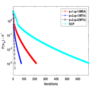
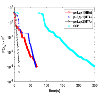
Figure 1: Behaviour of residual function for MTA with $q=2,p=1$ and with $q=p=2$, MBA and SCP along iterations (left) and time in sec (right): $n=100,m=10$.

		SCP		MBA[2] (MTA(1,1))		MTA(2,1)		MTA(2,2)
n	m	cpu	iter	cpu	iter	cpu	iter	cpu	iter
10	10	16.3	565	9.2	230	5.5	131	1.3	20
	20	24.5	458	9.8	149	4.2	64	2.5	23
	50	81.5	401	52.5	184	30.9	118	8.5	18
	100	428.7	818	145.6	246	55.2	90	25	19
	500	1119	146	534.7	50	252.8	27	135.9	9
	$10^{3}$	1.1$\cdot 10^{4}$	394	6.7$\cdot 10^{3}$	188	4.2$\cdot 10^{3}$	103	499.3	10
20	10	149.8	2477	40.7	700	25	243	13.5	84
	20	396.5	4134	166.9	1253	69.1	494	25.3	122
	50	544.5	1288	266.7	580	151.6	331	37.5	37
	100	862.4	551	441	243	264.2	148	72.3	23
	500	1.9$\cdot 10^{4}$	1078	$10^{4}$	454	5052	245	767.2	26
100	10	247	696	69.3	211	66	76	15.5	17
	20	6159	1179	713.3	306	350	79	252	28
	50	2.3$\cdot 10^{4}$	1460	5974	235	1026	25	711.3	18
	100	5.6$\cdot 10^{4}$	5611	$10^{4}$	1138	2055	89	1252	40
	500	$10^{6}$	1384	3$\cdot 10^{4}$	338	6325	67	2155	20

Table 2: Comparison between MTA with $q=2,p=1$ and with $q=p=2$, MBA and SCP in terms of iterations and cpu time (sec) for different values $m$ and $n$.

8 Conclusions

In this paper we have proposed a higher-order method for solving composite problems with smooth functional constraints. Our method uses higher-order derivatives to build a model that approximates the objective and the functional constraints. We have proved global convergence guarantees in both nonconvex and convex cases. We have also shown that our method is implementable and it is efficient in numerical simulations.

References

- [1] R. Andreani, J. M. Martínez and B. F. Svaiter, A new sequential optimality condition for constrained optimization and algorithmic consequences, SIAM Journal on Optimization, 20(6): 3533–3554, 2010.
- [2] A. Auslender, R. Shefi, and M. Teboulle, A moving balls approximation method for a class of smooth constrained minimization problems, SIAM Journal on Optimization, 20(6): 3232–3259, 2010.
- [3] J.W. Bandler, Optimization of design tolerances using nonlinear programming, Journal of Optimization Theory and Applications, 14(1): 99–114, 1974.
- [4] D. Bertsekas, Constrained Optimization and Lagrange Multiplier Methods, Academic Press, 1982.
- [5] D. Bertsekas, Nonlinear Programming, 2nd ed., Athena Scientific, Belmont, MA, 1999.
- [6] E. Birgin, J. Gardenghi, J. Martìnez, S. Santos and P. Toint, Evaluation complexity for nonlinear constrained optimization using unscaled KKT conditions and high-order models, SIAM Journal on Optimization, 26(2): 951–967, 2016.
- [7] E.G. Birgin, J.L. Gardenghi, J.M. Martinez, S.A. Santos, and P. L. Toint, Worst-case evaluation complexity for unconstrained nonlinear optimization using high-order regularized models, Mathematical Programming, 163: 359–368, 2017.
- [8] P.T. Boggs, and J.W. Tolle, Sequential quadratic programming, Act. Num., 4: 1–51, 1995.
- [9] J. Bolte, A. Daniilidis, A. Lewis and M. Shiota, Clarke subgradients of stratifiable functions, SIAM Journal on Optimization, 18(2): 556–572, 2007.
- [10] J. Bolte, Z. Chen and E. Pauwels, The multiproximal linearization method for convex composite problems, Mathematical Programming, 182: 1–36, 2020.
- [11] J. Bolte and E. Pauwels, Majorization-minimization procedures and convergence of SQP methods for semi-algebraic and tame programs, Math. Oper. Res., 41(2): 442–465, 2016.
- [12] J. Bolte, S. Sabach and M. Teboulle, Nonconvex Lagrangian-based optimization: monitoring schemes and global convergence, Math. Oper. Res., 43(4): 1210–1232, 2018.
- [13] C. Cartis, N.I.M. Gould and P.L. Toint, Universal regularized methods: varying the power, the smoothness and the accuracy, SIAM Journal on Optimization, 29(1): 595–615, 2019.
- [14] M. Chiang, C. Tan, D. Palomar, D. O. Neill and D. Julian, Power control by geometric programming, IEEE Trans. Wireless Commun., 6(7): 2640–2651, 2007.
- [15] C. Cartis, N.M. Gould and P.L. Toint, A concise second-order complexity analysis for unconstrained optimization using high-order regularized models, Optimization Methods and Software, 35(2): 243–256, 2020.
- [16] N. Doikov and Yu. Nesterov, Inexact tensor methods with dynamic accuracies, International Conference on Machine Learning, 2577–2586, 2020.
- [17] N. Doikov and Yu. Nesterov Optimization methods for fully composite problems, SIAM Journal on Optimization, 32(3): 2402–2427, 2022.
- [18] G.N. Grapiglia and Yu. Nesterov, Tensor methods for minimizing convex functions with Hölder continuous higher-order derivatives, SIAM Journal on Optimization, 30(4): 2750–2779, 2020.
- [19] M.R. Hestenes, Multiplier and gradient methods, Journal of Optimization Theory and Applications, 4: 303–320, 1969.
- [20] Y. Nabou, I. Necoara, Efficiency of higher-order algorithms for minimizing general composite functions, arXiv preprint: 2203.13367, 2022.
- [21] I. Necoara and D. Lupu, General higher-order majorization-minimization algorithms for (non) convex optimization, arXiv preprint: 2010.13893, 2020.
- [22] Yu. Nesterov and A. Nemirovskii, Interior-Point Polynomial Algorithms in Convex Programming, SIAM, Philadelphia, 1994.
- [23] Yu. Nesterov, Implementable tensor methods in unconstrained convex optimization, Mathematical Programming, 186: 157–183, 2021.
- [24] Yu. Nesterov and B.T. Polyak, Cubic regularization of Newton method and its global performance, Mathematical Programming, 108: 177–205, 2006.
- [25] D.P. Palomar and M. Chiang, Alternative decompositions for distributed maximization of network utility: framework and applications, IEEE Trans. Aut. Control, 52(12), 2007.
- [26] F. Messerer, K. Baumgärtner and M. Diehl, Survey of sequential convex programming and generalized Gauss-Newton methods, ESAIM: Proceedings and Surveys, 2021.
- [27] P. Rigollet and X. Tong, Neyman-pearson classification, convexity and stochastic constraints, Journal of Machine Learning Research, 12: 2831–2855, 2011.
- [28] A. Jr. Santos and G.R. Da Costa, Optimal-power-flow solution by Newton’s method applied to an augmented Lagrangian function, IEEE Proceedings - Generation, Transmission and Distribution, 142(1): 33–36, 1995.
- [29] P. Shen and K. Zhang, Global optimization of signomial geometric programming using linear relaxation, Applied Mathematics and Computation, 150: 99–114, 2004.
- [30] A. Wächter and L.T. Biegler, On the implementation of a primal-dual interior point filter line search algorithm for large-scale nonlinear programming, Math. Prog., 106: 25–57, 2006.
- [31] P. Yu, T.K. Pong and Z. Lu, Convergence Rate Analysis of a Sequential Convex Programming Method with Line Search for a Class of Constrained Difference-of-Convex Optimization Problems, SIAM Journal on Optimization, 31(3): 2024–2054, 2021.
- [32] D. Zhou, P. Xu and Q. Gu, Stochastic variance-reduced cubic regularized Newton methods, International Conference on Machine Learning, 5990–5999, 2018.
- [33] G. Zoutendijk, Method of Feasible Directions, Elsevier, Amsterdam, 1960.