Microscopic bell-shape nonlocality: the case of proton scattering off ⁴⁰Ca at 200 MeV

Abstract

This work is part of an ongoing effort to build microscopically-driven nonlocal optical potentials easily tracktable in scattering codes. Based on the separable ‘$JvH$’ structure proposed recently arellano_22 , where the potential can be cast as the product of a radial and nonlocality form factors, we investigate its angular dependence in momentum space. We find that scattering observables have a weak angular dependence between the momentum transfer $\bm{q}=\bm{k}-\bm{k}^{\prime}$, and $\bm{K}=(\bm{k}+\bm{k}^{\prime})/2$. The study is focussed on proton elastic scattering off ⁴⁰Ca at 200 MeV, where the $JvH$ structure is found to be inadequate. We conclude that any improvement of the $JvH$ structure of the potential can be made to the lowest order in multipole expansions in $Kq-$representation of the potential.

1 Introduction

In the early sixties, Perey and Buck (PB) proposed a phenomenological nonlocal optical potential for neutron scattering off spherical nuclei perey_62 . This potential factorizes into a Gaussian nonlocal form factor and a Woods-Saxon radial shape. The PB potential model has been further used as a starting point for numerous phenomenological studies. In addition to its extension to proton projectiles tian_15 , its imaginary component has been made energy dependent lovell_17 ; jaghoub_18 and also dispersive mahzoon_14 ; mahzoon_17 ; atkinson_20 .

In a previous work arellano_22 , we have studied microscopic optical model potentials based on a $g$-matrix approach arellano_89 , where the potential can be reduced to lowest order to the so-called $JvH$ form which relates directly to PB form factor. The work is done in momentum space, where a simplification is obtained with the use of mean momentum $\mathbf{K}$ and momentum transfer $\mathbf{q}$ instead of the usual $\mathbf{k}$ and $\mathbf{k^{\prime}}$ relative momenta. This $JvH$ potential is shown to reproduce elastic observables for incident energies up to 40 MeV.

In the present work we explore this microscopically-driven potential at 200 MeV incident energy. We start from microscopic potential based on a density-dependent infinite nuclear-matter model to represent the in-medium effective $NN$ interaction arellano_95 ; arellano_07a ; aguayo_08 , folded with proton and neutron densities from Gogny D1S Hartree-Fock calculations decharge_80 . The Brueckner-Hartree-Fock $g$-matrix is obtained using AV18 bare interaction wiringa_95 . We restrict this work to proton elastic scattering off ⁴⁰Ca at 200 MeV. In Sec. 2, we define two alternative representations: $kk^{\prime}$ and $Kq$, named after the coordinate system used. We truncate the angular dependence in the $Kq$-representation. The truncated potential is then expanded in $kk^{\prime}$ which is suitable to solve the scattering equations. The convergence of this multipolar expansion is assessed in Sec. 3. The underlying idea is to investigate whether lower orders in $Kq$-expansion retains the leading physics at 200 MeV incident energy. In Sec. 4, we assess the $JvH$ form for the optical potential. Limitations of the $JvH$ form relative to its original potential is illustrated in the context of elastic scattering.

Results from this work show that the $Kq$-representation exhibits a weak angular dependence between ${\bm{q}}$ and ${\bm{K}}$ allowing to focus on the term participating to $J$, $v$ and $H$ terms. This microscopically-driven potential should be tracktable for further phenomenology. Conclusions and perspectives are drawn in Sec. 5.

2 Expansions

We consider the general structure of the optical potential in momentum space. In all these approaches the optical potential for NA elastic scattering, ${\cal U}({\bm{k}}^{\prime},{\bm{k}};E)$, can be cast in the form arellano_22

$${\cal U}({\bm{k}^{\prime}},{\bm{k}};E)={\cal U}_{c}({\bm{k}^{\prime}},{\bm{k}})+i{\bm{\sigma}}\cdot\hat{\bm{n}}\,{\cal U}_{so}({\bm{k}^{\prime}},{\bm{k}})\;,$$ (1)

with $\hat{\bm{n}}$ the unit vector perpendicular to the scattering plane given by

$$\hat{\bm{n}}=\frac{\bm{k}^{\prime}\times\bm{k}}{|\bm{k}^{\prime}\times\bm{k}|}\,,$$ (2)

and ${\bm{\sigma}}$ the spin of the projectile. Here ${\cal U}_{c}$ and ${\cal U}_{so}$ represent the central and spin-orbit components of the potential. From now on, dependences on the energy $E$ are implicit. One can expand the potential in Eq. (1) in terms of relative momenta, $k$ and $k^{\prime}$, and the angle between ${\bm{k}}$ and ${\bm{k}}^{\prime}$ expressed by $u\!=\!\hat{\bm{k}}\cdot\hat{\bm{k}}^{\prime}$, as

$${\cal U}({\bm{k}^{\prime}},{\bm{k}})=\sum_{l=0}^{\infty}U_{l}(k,k^{\prime})P_{l}(u).$$ (3)

In the following, this expansion is referred to as $kk^{\prime}-$expansion, where $l$ represents the orbital angular momentum joachain_75 . This is the form we use to obtain the scattering observables using SWANLOP code arellano_21b that allows treatment of optical potential in momentum space as input.
Let us now define the following alternative variables,

$${\bm{K}}= \textstyle{\frac{1}{2}}({\bm{k}}+{\bm{k}}^{\prime}),$$ (4)

$${\bm{q}}= {\bm{k}}-{\bm{k}}^{\prime},$$ (5)

$$w= \hat{\bm{K}}\cdot\hat{\bm{q}},$$ (6)

with ${\bm{K}}$ the mean momentum and ${\bm{q}}$ the momentum transfer. We observe that ${\bm{k}^{\prime}}\times{\bm{k}}\!=\!{\bm{K}}\times{\bm{q}}$. As done in Ref. arellano_22 , we investigate the structure of the potential in terms of ${\bm{K}}$ and ${\bm{q}}$. Accordingly, we introduce the notation,

$${\cal U}({\bm{k}^{\prime}},{\bm{k}};E)={U}({\bm{K}},{\bm{q}})={U}_{c}(K,q,w)+i{\bm{\sigma}}\cdot({\bm{K}}\times{\bm{q}})\,{U}_{so}(K,q,w)\;.$$ (7)

Now we consider the following expansions,

$${U}_{c}(K,q,w) =\sum_{\begin{subarray}{c}n=0\\ n\ even\end{subarray}}^{N}\,{U}^{(c)}_{n}(K,q)P_{n}(w)\;,$$ (8a)

$$|{\bm{K}}\times{\bm{q}}|{U}_{so}(K,q,w) =Kq\sum_{\begin{subarray}{c}n=0\\ n\ even\end{subarray}}^{N}\,{U}^{(so)}_{n+1}(K,q)P^{1}_{n+1}(w)\;,$$ (8b)

for the central part and the spin-orbit potentials, respectively. In principle $N\!\rightarrow\!\infty$, but in practice we choose an upper limit. $P^{m}_{n}(w)$ is the associated Legendre polynomials. These expansions are referred to as $Kq-$expansion. Restriction of summation to even $n$ values in the central term comes from symmetry considerations. Note that the spin orbit term is summed over odd values. Details of spin-orbit derivations in Eq. (8b) can be found in Appendix A.

3 Convergence

We now explore the ability of different $Kq-$truncations to reproduce the full potential result in the context of the test case: proton elastic scattering off ⁴⁰Ca at 200 MeV. First of all, we verify that the exact results are reproduced when using high values of $N$.

In Fig. 1, we present the calculated differential cross sections obtained from full potential as in Eq. (1). We also show results considering the cases $N\!=\!0$, and $N\!=\!2$ from Eqs. (8a) and (8b). We observe that the agreement between the full calculation and that obtained for $N\!=\!0$, is already remarkable. The result for $N\!=\!2$ overlaps perfectly to the eye with the full calculation. For the sake of scrutinity, we include an inset where the differential cross section is plotted in linear scale, to strengthen this statement. In Table 1, we summarize the calculated reaction cross sections considering the full representation of the potential and its expressions up to $N\!=\!0$ and $2$. The difference between the full potential and the case of $N\!=\!0$ is about 0.4 %, reaching agreement up to four significant figures in the case of $N\!=\!2$. These results validate considering the former case as starting point.

Scheme	$\sigma_{R}$ [mb]
Full	526.5
$N\!=\!0$	528.4
$N\!=\!2$	526.5

Table 1: Reaction cross sections for p+⁴⁰Ca at 200 MeV for the full potential scattering calculation, the $N\!=\!0$ and $N\!=\!2$ truncations in the $Kq-$representation.

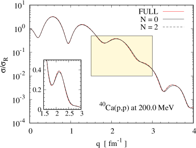
Figure 1: Ratio-to-Rutherford differential cross section as a function of the momentum transfer for p + ⁴⁰Ca at 200 MeV. Red curves correspond to the full potential, whereas solid and dashed black curves represent results in $Kq-$repesentation truncated at $N\!=\!0$ and $2$, respectively. The inset shows a close-up in linear scale.

4 $JvH$ and beyond

We have shown that the optical potential in the $Kq-$representation exhibits a weak dependence on the angle between $\bm{K}$ and $\bm{q}$. Actually, the truncation up to $N\!=\!0$ is reasonably good to retain the leading features present in the original potential in $kk^{\prime}-$representation. This feature justifies to focus on the $N\!=\!0$ truncated expansion of the potential. In this case Eqs. (8a) and (8b) become

$${U}_{c}(K,q,w) \approx{U}^{(c)}_{n=0}(K,q)\;,$$ (9a)

$${U}_{so}(K,q,w) \approx{U}^{(so)}_{n=1}(K,q)\,.$$ (9b)

Note that both terms are independent of $w$, namely the angle between ${\bm{K}}$ and ${\bm{q}}$. Following Ref.arellano_22 we define

$$V^{(c)}(K,q) =\frac{U_{c}(K,q)}{U_{c}(K,0)},$$ (10a)

$$H^{(c)}(K) =\frac{U_{c}(K,0)}{U_{c}(0,0)}.$$ (10b)

The term $U_{c}(0,0)$ is directly related to the volume integral through, $J^{(c)}=(2\pi)^{3}U_{c}(0,0)$. The same construction is applied to the spin-orbit term. Below $E\!=\!40$ MeV, $V^{(c)}$ and $V^{(so)}$ are $K$-independent arellano_22 . This is the key point to recover the Perey-Buck separability between a nonlocal form factor and a radial shape. Therefore we introduce the radial form factors,

$$V^{(c)}(K,q) \approx V^{(c)}(0,q)\equiv v^{(c)}(q)\,,$$ (11)

$$V^{(so)}(K,q) \approx V^{(so)}(0,q)\equiv v^{(so)}(q)\,.$$ (12)

In this way one gets the $JvH$ form of the potential,

$$U^{JvH}(K,q)=\frac{J^{(c)}}{(2\pi)^{3}}\,v^{(c)}(q)\,H^{(c)}(K)+i{\bm{\sigma}}\cdot({\bm{K}}\times{\bm{q}})\frac{J^{(so)}}{(2\pi)^{3}}\,v^{(so)}(q)\,H^{(so)}(K).$$ (13)

The behavior of the nonlocality of the microscopic optical potential is illustrated in Fig. 2, where we plot the nonlocality form factor $H$ as a function of $K$. Black and red curves correspond to the central and spin-orbit nonlocality form factors extracted from the microscopic optical potential, respectively. Solid and dashed curves correspond to their real (Re) and imaginary (Im) components, respectively. Here we also include the nonlocality form factor proposed by Perey-Buck perey_62 , namely

$$H^{PB}(K)=e^{-\beta^{2}K^{2}/4}\;,$$ (14)

where the nonlocality parameter is taken as $\beta\!=\!0.85$ fm.

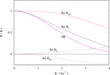
Figure 2: Bell-shape nonlocality form factor $H(K)$ in Eq. (13) for p + ⁴⁰Ca potential at 200 MeV. Results for central (c) and spin-orbit (so) compared with Perey-Buck nonlocality form factor with $\beta\!~{}=~{}\!0.85$ fm in Eq. (14).

We observe two features worth mentioning. First, the microscopic nonlocality form factor is complex, with a small imaginary contribution at the origin but increasing in magnitude as $K$ increases. Second, the curvature of $H$ at the origin is a measure of the range of the nonlocality. Thus, the nonlocality of the spin-orbit term is smaller than that in the central part. Interestingly, the curvature of the central potential and PB appear comparable.

In Fig. 3, we show results for the ratio-to-Rutherford differential cross sections $\sigma/\sigma_{R}$, analyzing power $A_{y}$ and spin-rotation $Q$ as functions of the momentum transfer $q$. The data are taken from Refs. hutcheon_88 and stephenson_85 . Red solid curves represent results based on the full potential. Black dashed curves correspond to $Kq-$representation considering $N\!=\!0$. These results illustrate the close correspondence between the full potential and its $Kq-$representation up to $N\!=\!0$, whereas clear differences are evidenced when compared to the $JvH$ form. Thus, the origin of these differences can be traced back to the use of Eqs. (11) and (12), where the $K$ dependence is neglected. This observation indicates that any improvement of the $JvH$ factorization would require corrections in $K$ at this level. Work along this line is underway.

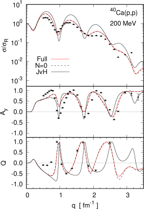
Figure 3: Ratio-to-Rutherford differential cross section, analyzing power and spin rotation as functions of the momentum transfer for p + ⁴⁰Ca elastic scattering at 200 MeV. Red solid curves are based on the full potential. Black dashed curves are based on its $Kq-$representation of order zero. Black solid curves represent results based on its $JvH$ factorization. The data are taken from Refs. hutcheon_88 and stephenson_85 .

5 Conclusions

The main result of this work is that $Kq-$representation of the optical model potential retains the main physics at its zero-th multipolar order. This feature is unveiled from a microscopic optical model potentials based on realistic bare nucleon-nucleon potentials. Although the $JvH$ form has been validated at low incident energies in Ref. arellano_22 , its limitations above 100 MeV can be corrected after a close scrutiny of the $K$ dependance in Eqs. (11) and (12). The long term aim of this effort is to provide guidance to phenomenomogical constructions of optical potentials resulting from detailed microscopic approaches.

Appendix A Spin-orbit term

We describe in details how to get the expansion for the spin-orbit contribution in Eq. (8a). We start from the usual expression of the spin-orbit,

$$\hat{U}=\hat{U}_{so}\,{\bm{\ell}}\cdot{\bm{\sigma}}\;.$$

Then we get the $kk^{\prime}-$representation of the potential,

$$\langle{\bm{k}^{\prime}}|\hat{U}|{\bm{k}}\rangle =\langle{\bm{k}^{\prime}}|\hat{U}_{so}\,{\bm{\ell}}\cdot{\bm{\sigma}}|{\bm{k}}\rangle$$ (15)

$$=\langle{\bm{k}^{\prime}}|\hat{U}_{so}\,i\hbar({\bm{r}}\times{\bm{p}})\cdot{\bm{\sigma}}|{\bm{k}}\rangle$$ (16)

$$=i\hbar\langle{\bm{k}^{\prime}}|\hat{U}_{so}\,\nabla_{k}\times{\bm{k}}\,|{\bm{k}}\rangle\cdot{\bm{\sigma}}.$$ (17)

Denote with $\partial_{i}$ the partial derivative with respect to the $i$-th component of momentum ${\bm{k}}$, we get

$$\langle{\bm{k}^{\prime}}|\hat{U}|{\bm{k}}\rangle =i\hbar\sum_{n}\epsilon_{imn}\partial_{i}\left(k_{m}\langle{\bm{k}^{\prime}}|\hat{U}_{so}\,|{\bm{k}}\rangle\right){\sigma}_{n}$$ (18)

$$=i\hbar\sum_{n}\epsilon_{imn}k_{m}\partial_{i}\left(\langle{\bm{k}^{\prime}}|\hat{U}_{so}\,|{\bm{k}}\rangle\right){\sigma}_{n}$$ (19)

$$=i\hbar\sum_{n}\epsilon_{nim}{\sigma}_{n}\partial_{i}\left(\langle{\bm{k}^{\prime}}|\hat{U}_{so}\,|{\bm{k}}\rangle\right)k_{m}$$ (20)

$$=i\hbar{\bm{\sigma}}\cdot\left(\nabla\langle{\bm{k}^{\prime}}|\hat{U}_{so}\,|{\bm{k}}\rangle\right)\times{\bm{k}}.$$ (21)

Let us define,

$$\langle{\bm{k}^{\prime}}|\hat{U}_{so}\,|{\bm{k}}\rangle=\sum_{l}U_{l}(k^{\prime},k)P_{l}(\hat{k}\cdot\hat{k}^{\prime}),$$

with ${\bm{k}^{\prime}}$ the azimuthal, then the non vanishing contribution above comes from angular variations in $\cos\theta=\hat{k}\cdot\hat{k}^{\prime}$. Hence

$$\langle{\bm{k}^{\prime}}|\hat{U}|{\bm{k}}\rangle =i\hbar{\bm{\sigma}}\cdot\left(\nabla\langle{\bm{k}^{\prime}}|\hat{U}_{so}\,|{\bm{k}}\rangle\right)\times{\bm{k}}$$ (22)

$$=i\hbar{\bm{\sigma}}\cdot\left(\frac{\partial}{k\,\partial\theta}\left[\sum_{l}U_{l}(k^{\prime},k)P_{l}(\hat{k}\cdot\hat{k}^{\prime})\right]\hat{\theta}\right)\times{\bm{k}}$$ (23)

$$=i\hbar{\bm{\sigma}}\cdot(\hat{\theta}\times\hat{k})\left(\frac{\partial}{\partial\theta}\left[\sum_{l}U_{l}(k^{\prime},k)P_{l}(\hat{k}\cdot\hat{k}^{\prime})\right]\right)$$ (24)

$$=i\hbar{\bm{\sigma}}\cdot\hat{n}\left(\sum_{l}U_{l}(k^{\prime},k)P_{l}^{1}(\hat{k}\cdot\hat{k}^{\prime})\right),$$ (25)

where we identify

$$\hat{n}=\frac{{\bm{k}^{\prime}}\times{\bm{k}}}{|{\bm{k}^{\prime}}\times{\bm{k}}|},$$

and

$$P_{l}^{1}(\cos\theta)=-\sin\theta\,\frac{dP_{l}(u)}{du},$$

with $P_{l}^{m}(x)$ the associated Legendre polynomials.

References

- (1) H.F. Arellano, G. Blanchon, The European Physical Journal A 58, 119 (2022)
- (2) F. Perey, B. Buck, Nucl. Phys. 32, 353 (1962)
- (3) Y. Tian, D.Y. Pang, Z.Y. Ma, International Journal of Modern Physics E 24, 1550006 (2015)
- (4) A.E. Lovell, P.L. Bacq, P. Capel, F.M. Nunes, L.J. Titus, Phys. Rev. C 96, 051601 (2017)
- (5) M.I. Jaghoub, A.E. Lovell, F.M. Nunes, Phys. Rev. C 98, 024609 (2018)
- (6) M.H. Mahzoon, R.J. Charity, W.H. Dickhoff, H. Dussan, S.J. Waldecker, Phys. Rev. Lett. 112, 162503 (2014)
- (7) M.H. Mahzoon, M.C. Atkinson, R.J. Charity, W.H. Dickhoff, Phys. Rev. Lett. 119, 222503 (2017)
- (8) M.C. Atkinson, W.H. Dickhoff, M. Piarulli, A. Rios, R.B. Wiringa, Phys. Rev. C 102, 044333 (2020)
- (9) H.F. Arellano, F.A. Brieva, W.G. Love, Phys. Rev. Lett. 63, 605 (1989)
- (10) H.F. Arellano, F.A. Brieva, W.G. Love, Phys. Rev. C 52, 301 (1995)
- (11) H.F. Arellano, M. Girod, Phys. Rev. C 76, 034602 (2007)
- (12) F.J. Aguayo, H.F. Arellano, Phys. Rev. C 78, 014608 (2008)
- (13) J. Dechargé, D. Gogny, Phys. Rev. C 21, 1568 (1980)
- (14) R.B. Wiringa, V.G.J. Stoks, R. Schiavilla, Phys. Rev. C 51, 38 (1995)
- (15) C.J. Joachain, Quantum Collision Theory (North-Holland Publishing Company, Amsterdam, 1975)
- (16) H.F. Arellano, G. Blanchon, Comp. Phys. Comm. 259, 107543 (2021)
- (17) D. Hutcheon, W. Olsen, H. Sherif, R. Dymarz, J. Cameron, J. Johansson, P. Kitching, P. Liljestrand, W. McDonald, C. Miller et al., Nuclear Physics A 483, 429 (1988)
- (18) E.J. Stephenson, J. Phys. Soc. Jpn. Conf. Proc. (Suppl.) 55, 316 (1985)