Repro Samples Method for a Performance Guaranteed Inference in General and Irregular Inference Problems

Abstract

Rapid advancements in data science require us to have fundamentally new frameworks to tackle prevalent but highly non-trivial “irregular” inference problems, to which the large sample central limit theorem does not apply. Typical examples are those involving discrete or non-numerical parameters and those involving non-numerical data, etc. In this article, we present an innovative, wide-reaching, and effective approach, called repro samples method, to conduct statistical inference for these irregular problems plus more. The development relates to but improves several existing simulation-inspired inference approaches, and we provide both exact and approximate theories to support our development. Moreover, the proposed approach is broadly applicable and subsumes the classical Neyman-Pearson framework as a special case. For the often-seen irregular inference problems that involve both discrete/non-numerical and continuous parameters, we propose an effective three-step procedure to make inferences for all parameters. We also develop a unique matching scheme that turns the discreteness of discrete/non-numerical parameters from an obstacle for forming inferential theories into a beneficial attribute for improving computational efficiency. We demonstrate the effectiveness of the proposed general methodology using various examples, including a case study example on a Gaussian mixture model with unknown number of components. This case study example provides a solution to a long-standing open inference question in statistics on how to quantify the estimation uncertainty for the unknown number of components and other associated parameters. Real data and simulation studies, with comparisons to existing approaches, demonstrate the far superior performance of the proposed method.

Key words: Artificial (Monte-Carlo) data; Conformal inference; Discrete or non-numerical parameters; Gaussian mixture; Generative model; Inversion method; Parametric and nonparametric settings

1 Introduction

The approaches of repeatedly creating Monte-Carlo (artificial) data to help assess uncertainty and make statistical inference have proven to be an effective method in the literature; see, e.g., Efron and Tibshirani (1993); Fishman (1996); Robert (2016); Hannig et al. (2016), and references therein. Most of these approaches, however, rely on the large sample central limit theorem (CLT) or related works to justify their inference validity. Their applicability to more complicated problems, especially those involving discrete or non-numerical parameters and non-numerical data (e.g., the unknown number of clusters; models A, B, …; architecture parameters (layers/number of neurons) in neural networks; space partitions in tree models; graphical network models; population ranks; etc.), is limited. In this article, we develop a fundamentally new and wide-reaching artificial-sample-inspired inferential framework and provide comprehensive supporting theories that can be used for such complicated problems plus more. The proposed framework, called repro samples method, does not need to rely on large sample theories or likelihood functions. It is especially effective for difficult irregular inference problems. Here, following wasserman2020universal, the irregular inference problems refer to those “highly non-trivial” and “complex setups” to which the regularity assumptions (for large sample theories) do not apply. Although our focus is mostly on finite-sample inference, the proposed framework has direct extensions to the situations where the large sample theorem does hold.

Suppose that the sample data $\bm{Y}\in{\cal Y}$ are generated from a model or a distribution $\bm{Y}|{\mathop{\theta\kern-4.49997pt\hbox{$\theta$}}\nolimits}_{0}\sim F_{{\bf\theta}_{0}}(\cdot),$ where ${\mathop{\theta\kern-4.49997pt\hbox{$\theta$}}\nolimits}_{0}\in\Theta$ is the true value of the model parameters that can either be numerical, or non-numerical, or a mixture of both. The sample data $\bm{Y}$ typically contain $n$ observations $\bm{Y}=(Y_{1},\ldots,Y_{n})^{\top}$ as in most publications, but in this paper we also allow $\bm{Y}$ to be a summary or function of $\bm{Y}$, or even non-numerical types of data (e.g., image; voice; object data; etc.). We assume only that we know how to simulate $\bm{Y}$ data from $F_{\bf\theta}(\cdot)$, given $\mathop{\theta\kern-4.49997pt\hbox{$\theta$}}\nolimits$. Often, $\bm{Y}|{\mathop{\theta\kern-4.49997pt\hbox{$\theta$}}\nolimits}\sim F_{{\bf\theta}}(\cdot)$ can be re-expressed in the form of generative algorithmic model:

$$\bm{Y}=G({\mathop{\theta\kern-4.49997pt\hbox{$\theta$}}\nolimits},\bm{U}),$$ (1)

where $G(\cdot,\cdot)$ is a known mapping from $\Theta\times{\cal U}\mapsto{\cal Y}$ and $\bm{U}=(U_{1},\ldots U_{r})^{\top}\in{\cal U}$, for some $r>0$, is a random vector whose distribution is free of $\bm{\theta}$. Let

$$\bm{y}_{obs}=G({\mathop{\theta\kern-4.49997pt\hbox{$\theta$}}\nolimits}_{0},\bm{u}^{rel})$$

be the realized observation and $\bm{u}^{rel}$ be the corresponding (unobserved) realization of $\bm{U}$. The algorithmic model formulation (1) is common in the literature (e.g., dalmasso2022; Robert2016; Hannig2016; Martin2015). It is very general. For instance, it can be a machine learning generative model or a differential equation based model. It also subsumes the traditional statistical models specified using a (parametric) family of density functions.

The repro samples framework relies on a simple yet fundamental idea: study the performance of artificial samples obtained by mimicking the sampling mechanism of the observed data; then use them to help quantify inference uncertainty. The intuition is that, if an artificial sample, say $\bm{y}^{*}$, generated using a $\mathop{\theta\kern-4.49997pt\hbox{$\theta$}}\nolimits\in\Theta$ can match well with the observed $\bm{y}_{obs}$, then we cannot dismiss the possibility that such a $\mathop{\theta\kern-4.49997pt\hbox{$\theta$}}\nolimits$ equals $\mathop{\theta\kern-4.49997pt\hbox{$\theta$}}\nolimits_{0}$. In particular, for any $\mathop{\theta\kern-4.49997pt\hbox{$\theta$}}\nolimits\in\Theta$ and a copy of $\bm{u}^{*}\sim\bm{U}$, we can use equation (1) to get a copy of artificial sample $\bm{y}^{*}=G({\mathop{\theta\kern-4.49997pt\hbox{$\theta$}}\nolimits},\bm{u}^{*})$, which we refer to in this paper as a repro sample. When $\mathop{\theta\kern-4.49997pt\hbox{$\theta$}}\nolimits=\mathop{\theta\kern-4.49997pt\hbox{$\theta$}}\nolimits_{0}$ and $\bm{u}^{*}$ matches $\bm{u}^{rel}$, the corresponding $\bm{y}^{*}$ will match $\bm{y}_{obs}$. The obstacle is that both $\mathop{\theta\kern-4.49997pt\hbox{$\theta$}}\nolimits_{0}$ and $\bm{u}^{rel}$ are unknown. However, we can use the fact that $\bm{u}^{rel}$ and $\bm{u}^{*}$ are both realizations from the same $\bm{U}$ distribution (and also a so-called nuclear mapping function to be introduced in Section 2) to first quantify $\bm{u}^{*}$. For the collection of $\bm{u}^{*}$’s that have a relative high possibility of being a potential candidate of $\bm{u}^{rel}$, we find those $\mathop{\theta\kern-4.49997pt\hbox{$\theta$}}\nolimits$ values that can produce repro samples $\bm{y}^{*}=G(\mathop{\theta\kern-4.49997pt\hbox{$\theta$}}\nolimits,\bm{u}^{*})$ that match $\bm{y}_{obs}$. Our proposal is to use such $\mathop{\theta\kern-4.49997pt\hbox{$\theta$}}\nolimits$’s to recover and make inference for $\mathop{\theta\kern-4.49997pt\hbox{$\theta$}}\nolimits_{0}$. The repro samples method is broadly applicable for any, including the complex irregular, inference problems.

In this paper, we formally formulate the above idea to develop a general framework to construct level-$\alpha$ confidence sets, $\alpha\in(0,1)$, for parameters of interest in the generative model (1) and a generalized semiparametric model setup. The development covers both regular and irregular problems and also both finite and large sample settings. We show that confidence sets constructed by the method have theoretically guaranteed frequency coverage rates. Furthermore, most inference problems in statistics applications and machine learning models often involve nuisance parameters and are complicated. We further provide several theoretical developments on handling nuisance parameters, the use of a data-driven candidate set to reduce computing costs, among others. We also show that the traditional Neyman-Pearson test procedure can be viewed as a special case of the proposed framework, in the sense that the confidence sets obtained by the repro samples method are never worse than (i.e., either the same as or smaller than) the confidence sets constructed by the Neyman-Pearson procedure. This framework is effective and it overcomes (or sidesteps) several drawbacks of several existing simulation-based inference approaches.

The repro samples method is particularly useful for irregular inference problems, which are prevalent and “highly non-trivial” (cf., wasserman2020universal; Xie2009). For these problems, point estimators (if exist) do not provide uncertainty quantification, and the often-used bootstrap approaches lack theoretical support. Bayesian methods may construct credible sets, but the sets are highly sensitive to the prior choices and their frequency coverage performance is typically poor even when the sample sizes are large (hastie2012; Kass1995). These difficulties are because the large sample CLT and Bernstein-von-Mises (BvM) theorem do not apply in these irregular cases. On the contrary, the repro samples method can be used to solve the difficult inference problems. In this paper, we specifically proposed and highlight an effective three-step procedure to handle irregular inference problems with model parameters $\mathop{\theta\kern-4.49997pt\hbox{$\theta$}}\nolimits=(\eta,{\bm{\beta}}^{\top})^{\top}$, where $\eta$ are discrete or non-numerical parameters and, when given $\eta$, the remaining parameters $\bm{\beta}$ may be handled by a regular approach. This three-step approach dissects a complicated irregular inference problem into manageable steps. Furthermore, the discrete nature of $\eta,$ an obstacle in developing inference theories, transforms into a beneficial attribute within our repro samples framework, to greatly improve computational and inference efficiency.

Major contributions and significance.

1. We develop a novel and broadly applicable inferential framework to construct performance-guaranteed confidence sets for parameters of interest under a general generative model. The proposed framework is likelihood-free and general. In addition to the regular inference problems under the conventional settings, the method is particularly useful for irregular inference problems and can effectively handle discrete or non-numerical parameters and non-numerical data. (Sections 2-6)

2. We introduce a so-called nuclear mapping function to greatly increase the flexibility and utility of the proposed method. A nuclear mapping function plays a similar role as a test statistic but is more general and does not need to be a test statistic. In the special case where the nuclear mapping function is a test statistic, we show that a confidence set obtained by the repro samples method is always better than (either the same as or smaller than) that obtained by inverting the Neyman-Pearson test procedure. We obtain optimality results that an optimal Neyman-Pearson method correspond to optimal confidence sets by the repro samples method; we also provide examples that the repro samples method improves the result by a Neyman-Pearson method when it is not optimal. (Sections 2.1 & 6)

3. Although the repro samples method is a simulation-inspired method, it can provide explicit mathematical solutions without involving simulation in many cases. In the cases when an explicit expression is unavailable, we develop effective algorithms to compute confidence sets using simulated samples. To reduce computing costs, we develop a novel data-driven approach, with supporting theories, to significantly reduce the search space of discrete/non-numerical parameters, by utilizing a many-to-one mapping that is unique in repro samples. For continuous parameters, we can use a quantile regression technique similar to that described in dalmasso2022. (Sections 2.2, 3.2 & Appendix)

4. We develop a novel profiling method to handle nuisance parameters under the proposed repro samples framework. Unlike the conventional ‘hybrid’ or ‘likelihood profiling’ methods that often rely on asymptotics (e.g., Chuang2000; dalmasso2022), the proposed method is developed based on $p$-values constructed under the repro samples framework, and it guarantees the finite sample coverage rates of the constructed confidence sets for the target parameters. The approach is computationally efficient and effective for many complex irregular inference problems. (Sections 3.1 & 4)

5. We provide a case study example to demonstrate the effectiveness of the repro samples method in handling irregular inference problems with varying number of parameters. Specifically, we provide a solution to an open and “highly nontrivial” inference problem in statistics on how to quantify the uncertainty in estimating the unknown number of the components (say $\tau_{0}$) and also associated parameters in a Gaussian mixture model (cf. wasserman2020universal; chen_inference_2012). Numerical studies, comparing with existing frequentist and Bayesian approaches, show that the repro samples method is the only effective approach that can always cover $\tau_{0}$ with the desired accuracy. (Section 4)

6. The repro samples framework stems from several simulation-based approaches across Bayesian, frequentist and fiducial (BFF) paradigms, namely, bootstrap, approximate Bayesian computing (ABC), generalized fiducial inference (GFI) and inferential model (IM), but it addresses or sidesteps several drawbacks of these existing approaches. Moreover, it provides a unique perspective to bridge the foundation of statistical inference across BFF paradigms. As a purely frequentist approach, it is transformative both theoretically and practically and has unique strengths in many areas. (Section 1 & Appendix)

Relation to other work: Beside the classical Neyman-Pearson testing method (Item 2 above), there are several relevant inferential approaches in the literature. More details and additional discussions are provided in Appendix C.

Efron’s Bootstrap and related methods are perhaps the most successful and broadly-used artificial-sample-based inference approach to date. The key justification is the so-called bootstrap central limit theorem (Singh1981; Bickel1981) in which the randomness of resampling (multinomial-distributed) is matched with the sampling randomness of the data (often not-multinomial distributed) using the large sample central limit theorem. Instead of resampling, the repro samples method directly generates artificial samples using $\bm{u}^{*}$. It does not need any large sample theorems, and can effectively address many problems that the bootstrap methods cannot.

Approximate Bayesian Computing (ABC) methods refer to a family of techniques used to approximate posterior distributions of $\mathop{\theta\kern-4.49997pt\hbox{$\theta$}}\nolimits$ by bypassing direct likelihood evaluations (e.g., csillery2010approximate). Both ABC and repro samples methods look for artificial samples that are similar to $\bm{y}_{obs}$, but the repro samples method utilizes many copies of artificial samples at each parameter value while ABC typically uses only one copy. The repro samples method sidesteps two difficulties encountered in an ABC method, i.e., requiring a) the summary statistic used in an ABC algorithm be sufficient and b) a pre-specified approximation value $\epsilon\to 0$ at a fast rate as sample size $n\to\infty$ (Li2016). Furthermore, the repro samples method is a frequentist method and need not assume a prior distribution.

Generalized fiducial Inference (GFI) is a generalization of Fisher’s fiducial method, which is understood in contemporary statistics as an “inversion method” to solve a pivot equation for model parameter $\mathop{\theta\kern-4.49997pt\hbox{$\theta$}}\nolimits$ (Zabell1992; Hannig2016). A GFI method can be viewed as a constrained optimization method that limits artificial data within an $\epsilon$-neighborhood of $\bm{y}_{obs}$, and it relies on large-sample and the so-called fiducial Berstein-von-Mises theorem to justify its inference validity (Hannig2016). Different than the repro samples method, The GFI method has the same issue as the ABC method, requiring a pre-specified $\epsilon\to 0$ at a fast rate, as sample size $n\to\infty$. Furthermore, the repro samples method has a guaranteed finite-sample frequentist performance and can effectively handle irregular inference problems in which large-sample theorems do not apply.

Inferential Model (IM) is a new framework to produce an epistemic “prior-free exact probabilistic inference” for unknown parameter $\mathop{\theta\kern-4.49997pt\hbox{$\theta$}}\nolimits_{0}$ (Martin2015). A novel aspect of the IM method (beyond a typical fiducial procedure) is that inferential uncertainty is quantified through $\bm{U}$ in (1) using random sets. The repro samples method also uses the distribution of $\bm{U}$ for uncertainty quantification, but through a nuclear mapping function and a fixed level-$\alpha$ set. The repro samples method additionally stresses the actual matching of simulated $\bm{u}^{*}$ with the unknown $\bm{u}^{rel}$, leading to a novel method for obtaining a data-driven candidate set that is particularly useful for irregular inference problems. Unlike IM, the repro samples method is fully a frequentist approach without needing any additional probability system (e.g., Dempster-Shafer calculus, etc.). The repro samples methods can also cover large sample inferences. They are less restrictive, more flexible, and easier to implement than the IM method.

Universal inference is another novel framework developed for conducting performance-guaranteed inferences without regularity conditions (wasserman2020universal). The method typically requires a tractable likelihood function and data splitting. It relies on a Markov inequality to justify its validity (testing size), at some expanse of power (Dunn2022; TseDavison2023). The framework can handle irregular inference problems and is particularly effective for sequential testing problems (ramdas2020admissible; Xie2023Discussion). The case study example of Gaussian mixture is also studied in wasserman2020universal but, unlike the repro samples method, it cannot provide a two-sided confidence set for $\tau_{0}$. The repro samples method is a likelihood-free approach that is also effective for irregular inference problems. Unlike the universal inference method, it does not systemically suffer a loss of power while maintaining its inference validity.

Organization of the remaining sections

Section 2 develops a basic yet general framework of the repro samples method with supporting theories. Section 3 provides further developments, including handling of nuisance parameters, developing a data-driven candidate set to improve computational efficiency, and developing an effective three-step procedure tailored for irregular inference problems. Section 4 is a case study example that addresses a long-standing open inference problem in a Gaussian mixture model on how to quantify the estimation uncertainty of the unknown number of components in the mixture and make associate inference for other parameters. Section 5 contains a real data analysis and simulation studies that demonstrate the effectiveness of the proposed method. To better understand the scope of the proposed repro samples framework, we compare it with the classical Neyman-Pearson procedure in Section 6, showing that the repro samples method subsumes the classical method as a special case. Section 7 provides further remarks and some future research directions.

2 A general inference framework by repro samples

Let $(\Omega,{\cal F},\mathbb{P})$ be a probability space and $\bm{U}\in{\cal U}\subset\mathbb{R}^{r}$ is a measurable $r\times 1$ random vector with $\{\bm{U}\leq\bm{u}\}=\{\omega\in\Omega:\bm{U}(\omega)\leq\bm{u}\}$. For a given $\mathop{\theta\kern-4.49997pt\hbox{$\theta$}}\nolimits^{*}$ and a simulated $\bm{u}^{*}\sim\bm{U}$, we call $\bm{y}^{*}=G({\mathop{\theta\kern-4.49997pt\hbox{$\theta$}}\nolimits}^{*},\bm{u}^{*})$ an (artificial) repro sample of $\bm{y}_{obs}$ and $\bm{u}^{*}$ a repro copy of $\bm{u}^{rel}$. Section 2.1 presents a basic yet general framework of a repro samples method, including a nonparametric (semi-parametric) extension to which model (1) is not fully specified. Section 2.2 provides a generic algorithm to construct a confidence set for the cases when an explicit mathematical expression is not available.

2.1 A general formulation of a repro samples method

Under model (1), the sampling uncertainty of $\bm{Y}$ is solely determined by the uncertainty of $\bm{U}$, whose distribution is free of the unknown parameters $\mathop{\theta\kern-4.49997pt\hbox{$\theta$}}\nolimits_{0}$. As in Martin2015 we first focus on the easier task of quantifying the uncertainty of $\bm{U}$; however we use a single fixed level-$\alpha$ Borel set $B_{\alpha}\subset{\cal U}$. Specifically, let $B_{\alpha}$ be a set such that $\mathbb{P}\{\bm{U}\in B_{\alpha}\}\geq\alpha,$ for some $0<\alpha<1$ (e.g., $\alpha=.95$ or $.99$). It follows that we have more than $\alpha$-level confidence that $\bm{u}^{rel}\in B_{\alpha}$ for the realized unknown $\bm{u}^{rel}$ corresponding to $\bm{y}_{obs}$. We define

$$\Gamma_{\alpha}(\bm{y}_{obs})=\big{\{}\mathop{\theta\kern-4.49997pt\hbox{$\theta$}}\nolimits:\exists\,\bm{u}^{*}\in B_{\alpha}\mbox{ s.t. }\bm{y}_{obs}=G({\mathop{\theta\kern-4.49997pt\hbox{$\theta$}}\nolimits},\bm{u}^{*})\big{\}}\subset\bm{\Theta},$$ (2)

where s.t. is an abbreviation for such that. That is, for a potential value $\mathop{\theta\kern-4.49997pt\hbox{$\theta$}}\nolimits$, if there exists a $\bm{u}^{*}\in B_{\alpha}$ such that the repro sample ${\bm{y}}^{*}=G({\mathop{\theta\kern-4.49997pt\hbox{$\theta$}}\nolimits},{\bm{u}}^{*})$ matches with $\bm{y}_{obs}$ (i.e., $\bm{y}^{*}=\bm{y}_{obs}$), then we keep this $\mathop{\theta\kern-4.49997pt\hbox{$\theta$}}\nolimits$ in the set $\Gamma_{\alpha}(\bm{y}_{obs})$. Note that the observed sample $\bm{y}_{obs}$ can be produced by the pair $({\mathop{\theta\kern-4.49997pt\hbox{$\theta$}}\nolimits},\bm{u}^{*})$ with $\bm{u}^{*}$ being an realization of $\bm{U}$, so we cannot rule out the possibility of $\mathop{\theta\kern-4.49997pt\hbox{$\theta$}}\nolimits=\mathop{\theta\kern-4.49997pt\hbox{$\theta$}}\nolimits_{0}.$ Since $\bm{y}_{obs}=G({\mathop{\theta\kern-4.49997pt\hbox{$\theta$}}\nolimits}_{0},\bm{u}^{rel})$, if $\bm{u}^{rel}\in B_{\alpha}$ then $\mathop{\theta\kern-4.49997pt\hbox{$\theta$}}\nolimits_{0}\in\Gamma_{\alpha}(\bm{y}_{obs})$. Similarly, under the model $\bm{Y}=G({\mathop{\theta\kern-4.49997pt\hbox{$\theta$}}\nolimits}_{0},\bm{U})$, we have $\left\{\bm{U}\in B_{\alpha}\right\}\subseteq\left\{\mathop{\theta\kern-4.49997pt\hbox{$\theta$}}\nolimits_{0}\in\Gamma_{\alpha}(\bm{Y})\right\}$. Thus,

$$\mathbb{P}\left\{\mathop{\theta\kern-4.49997pt\hbox{$\theta$}}\nolimits_{0}\in\Gamma_{\alpha}(\bm{Y})\right\}\geq\mathbb{P}\big{\{}\bm{U}\in B_{\alpha}\big{\}}\geq\alpha.$$

Thus, by construction, the set $\Gamma_{\alpha}(\bm{y}_{obs})$ in (2) is a level-$\alpha$ confidence set for $\mathop{\theta\kern-4.49997pt\hbox{$\theta$}}\nolimits_{0}$.

To expand the scope of our framework, we propose to replace the requirement $\mathbb{P}(\bm{U}\in B_{\alpha})\geq\alpha$ by

$$\mathbb{P}\left\{T(\bm{U},\mathop{\theta\kern-4.49997pt\hbox{$\theta$}}\nolimits)\in B_{\alpha}(\mathop{\theta\kern-4.49997pt\hbox{$\theta$}}\nolimits)\right\}\geq\alpha,$$ (3)

for any fixed $\mathop{\theta\kern-4.49997pt\hbox{$\theta$}}\nolimits$, where $T(\cdot,\cdot)$ is a (given) mapping function from ${\cal U}\times\Theta\to$ ${\cal T}\subseteq\mathbb{R}^{q}$, for some $q\leq n$. Then, the constructed confidence set in (2) becomes

$$\Gamma_{\alpha}(\bm{y}_{obs})=\big{\{}\mathop{\theta\kern-4.49997pt\hbox{$\theta$}}\nolimits:\exists\,\bm{u}^{*}\in{\cal U}\mbox{ s.t. }\bm{y}_{obs}=G({\mathop{\theta\kern-4.49997pt\hbox{$\theta$}}\nolimits},\bm{u}^{*}),\,T(\bm{u}^{*},\mathop{\theta\kern-4.49997pt\hbox{$\theta$}}\nolimits)\in B_{\alpha}(\mathop{\theta\kern-4.49997pt\hbox{$\theta$}}\nolimits)\big{\}}\subset\Theta.$$ (4)

The mapping function $T$, which we refer to as a nuclear mapping, adds much flexibility to the proposed repro-samples method and is necessary for many more complicated problems, as we will see in the rest of the paper. For now, we assume that the nuclear mapping function $T$ is given. Further discussions on the choice of $T$ will be included in Sections 3 - 6. At the outset, we state that the role of the nuclear mapping $T$ is similar to, but broader than, that of a test statistic in the classical Neyman-Pearson testing framework.

Theorem 1 below states that the set $\Gamma_{\alpha}(\bm{y}_{obs})$ in (4) is a level-$\alpha$ confidence set, including both finite-sample exact inference and potential (large sample or other) approximations.

Theorem 1.

Assume model (1) holds with $\bm{\theta}=\bm{\theta}_{0}$. If inequality (3) holds exactly for any fixed $\bm{\theta}$, then the following inequality holds exactly

$$\mathbb{P}\left\{{\mathop{\theta\kern-4.49997pt\hbox{$\theta$}}\nolimits}_{0}\in\Gamma_{\alpha}(\bm{Y})\right\}\geq\alpha\,\,\,\hbox{for}\,\,0<\alpha<1.$$ (5)

Furthermore, if the inequality (3) holds approximately with $\mathbb{P}\big{\{}T(\bm{U},\mathop{\theta\kern-4.49997pt\hbox{$\theta$}}\nolimits)\in B_{\alpha}(\mathop{\theta\kern-4.49997pt\hbox{$\theta$}}\nolimits)\big{\}}\geq\alpha\{1+o(\delta^{{}^{\prime}})\}$, then (5) holds approximately with $\mathbb{P}\left\{{\mathop{\theta\kern-4.49997pt\hbox{$\theta$}}\nolimits}_{0}\in\Gamma_{\alpha}(\bm{Y})\right\}\geq\alpha\{1+o(\delta^{{}^{\prime}})\}$, for $0<\alpha<1$, where $\delta^{{}^{\prime}}>0$ is a small value that may or may not depend on sample size $n$.

A proof of the theorem is in Appendix A. In Theorem 1, the $\delta^{{}^{\prime}}$ may or may not depend on the sample size $n$. In examples involving large sample approximations, $\delta^{{}^{\prime}}$ is often a function of $n$ with $\delta^{{}^{\prime}}\to 0$ as $n\to 0$. However, there are also examples in which $\delta^{{}^{\prime}}$ does not involve $n$. For example, suppose that $Y|\theta=\lambda\sim\text{Poisson}(\lambda)$. Then, $U=(Y-\lambda)/\sqrt{\lambda}\to N(0,1)$, when $\lambda$ is large. So, if we take $T(U,\lambda)=U$, $\mathbb{P}\{T(U,\lambda)\in B\}=\int_{{t}\in B}\phi({t})d{t}\{1+o(\lambda^{-1})\}$, for any Borel set $B$; thus $\delta^{{}^{\prime}}=\lambda^{-1}$. Here, $\phi(t)$ is the density function of $N(0,1)$.

To illustrate the proposed repro samples method, we consider below a binomial example.

 Example 1.

[Binomial sample with small $\theta_{0}$] Assume $Y\sim Binomial(r,\theta_{0})$, $0<\theta_{0}<1$, and we observe $y_{obs}$. We can re-express the model as $Y=\sum_{i=1}^{r}{\bf 1}{(U_{i}\leq\theta_{0})}$ for $U_{1},\ldots,U_{r}\sim U(0,1)$. It follows that $y_{obs}=\sum_{i=1}^{r}{\bf 1}{(u_{i}^{rel}\leq\theta_{0})},$ where $\bm{u}^{rel}=(u_{1}^{rel},\ldots,u_{r}^{rel})$ is the realization of $\bm{U}=(U_{1},\ldots,U_{r})$ corresponding to $y_{obs}$.

For a given vector $\bm{u}=(u_{1},\ldots,u_{r})$, we consider the nuclear mapping function $T(\bm{u},\theta)=\sum_{i=1}^{r}{\bf 1}{(u_{i}\leq\theta)}$. We have $T(\bm{U},\theta)=\sum_{i=1}^{r}{\bf 1}{(U_{i}\leq\theta)}\sim Binomial(r,\theta)$, for each given $\theta\in\Theta=(0,1)$. Let $B_{\alpha}(\theta)$ in (3) be an interval $B_{\alpha}(\theta)=[a_{L}(\theta),a_{U}(\theta)]$, where the bounds

$$\left(a_{L}(\theta),a_{U}(\theta)\right)=\arg\min\nolimits_{\big{\{}(i,j):\sum^{j}_{k=i}{r\atopwithdelims( )k}\theta^{k}(1-\theta)^{(r-k)}\geq\alpha\big{\}}}|j-i|,$$ (6)

are the pair of $(i,j)$ in $\{(i,j):\sum^{j}_{k=i}{r\atopwithdelims( )k}\theta^{k}(1-\theta)^{(r-k)}\geq\alpha\}$ that makes the shortest interval $\left[a_{L}(\theta),a_{U}(\theta)\right]$. By a direct calculation, it follows that $P\left\{T(\bm{U},\theta)\in[a_{L}(\theta),a_{U}(\theta)]\right\}\geq\alpha$, for any $\theta\in(0,1)$; thus, equation (3) is satisfied. The confidence set in (4) is then

$$\Gamma_{\alpha}(y_{obs}) = \bigg{\{}\theta\big{|}\exists\,\bm{u}^{*}\in{\cal U}\,\hbox{s.t.}\,\,y_{obs}=\sum\nolimits_{i=1}^{r}{\bf 1}{(u_{i}^{*}\leq\theta)},\sum\nolimits_{i=1}^{r}{\bf 1}{(u_{i}^{*}\leq\theta)}\in[a_{L}(\theta),a_{U}(\theta)]\bigg{\}}$$

$$= \left\{\theta\big{|}y_{obs}=\sum\nolimits_{i=1}^{r}{\bf 1}{(u_{i}^{*}\leq\theta)},y_{obs}\in[a_{L}(\theta),a_{U}(\theta)],\exists\,\bm{u}^{*}\in{\cal U}\right\}$$

$$= \left\{\theta\big{|}y_{obs}=\sum\nolimits_{i=1}^{r}{\bf 1}{(u_{i}^{*}\leq\theta)},\exists\,\bm{u}^{*}\in{\cal U}\right\}\cap\left\{\theta\big{|}y_{obs}\in[a_{L}(\theta),a_{U}(\theta)]\right\}$$

$$= \left\{\theta\big{|}a_{L}(\theta)\leq y_{obs}\leq a_{U}(\theta)\right\}.$$

The last equation holds, because for any given $\theta\in\Theta=(0,1)$ there always exists at least a $\bm{u}^{*}\in{\cal U}$ such that $y_{obs}=\sum_{i=1}^{r}{\bf 1}{(u_{i}^{*}\leq\theta)}$, i.e., $\{\theta\big{|}y_{obs}=\sum_{i=1}^{r}{\bf 1}{(u_{i}^{*}\leq\theta)},\exists\,\bm{u}^{*}\in{\cal U}\}=\Theta$.

Table 1 provides a numerical study comparing the empirical performance of $\Gamma_{.95}(y_{obs})$ (Repro) against 95% confidence intervals obtained using the traditional Wald method and the fiducial approach (GFI) of Hannig2009, both of which are asymptotic methods that can ensure coverage only when $n$ is large. The rerpo sampling method is an exact method that improves the performance of existing methods, especially when $n\theta_{0}<5$ (a rule of thumb on asymptotic approximation of binomial data; cf., tCAS90a).

		$n=20,\theta_{0}=0.1$			$n=20,\theta_{0}=0.4$			$n=20,\theta_{0}=0.8$
		Coverage	Width		Coverage	Width		Coverage	Width
Repro		0.949(0.007)	0.281(0.059)		0.963(0.006)	0.408(0.026)		0.959(0.006)	0.342(0.045)
Wald		0.877(0.010)	0.236(0.052)		0.927(0.008)	0.418(0.028)		0.915(0.009)	0.332(0.071)
GFI		0.988(0.003)	0.293(0.065)		0.963(0.006)	0.438(0.022)		0.973(0.004)	0.365(0.056)

Table 1: Comparison of $95\%$ confidence intervals by the repro, Wald and GFI methods in Binomial$(n,\theta_{0})$ data; repetitions $=1000$; standard errors (sd’s) are enclosed in brackets.

Corollary 1 below states that the repro samples method can be used to test a hypothesis.

Corollary 1.

To test a hypothesis $H_{0}:\bm{\theta}\in\Theta_{0}$ vs $H_{1}:\bm{\theta}\not\in\Theta_{0}$, we can define a p-value

$$p(\bm{y}_{obs})=1-\inf\nolimits_{\bm{\theta}\in\Theta_{0}}\left[\inf\left\{\alpha:\bm{\theta}\in\Gamma_{\alpha}(\bm{y}_{obs})\right\}\right],$$

where $\Theta_{0}\subsetneq\Theta$ and $\Gamma_{\alpha}(\bm{y}_{obs})$ is defined in (4). Rejecting $H_{0}$ when $p(\bm{y}_{obs})\leq\gamma$ leads to a size $\gamma$ test, for any $0<\gamma<1$.

A proof of the corollary is in Appendix A. Section 6 further investigates the relationship between the repro samples method and the classical Neyman-Pearson testing procedure.

The repro samples method can also be applied in cases when model (1) is not fully available. For instance, consider a nonparametric problem of making inference for the $\zeta$-th quantile of a completely unknown distribution $F$, say, $\theta_{0}=F^{-1}(\zeta)$. If $Y\sim F$, we have $I(Y<\theta_{0})\sim\text{Bernoulli}(\zeta)$ and equation $I(Y<\theta_{0})=U$, where $U\sim\text{Bernoulli}(\zeta)$. Now suppose we observe data $\bm{y}_{obs}=(y_{1}\ldots,y_{n})^{\top}$, for a fixed $n$, then the equation becomes

$$\sum_{i=1}^{n}I(Y_{i}-\theta_{0}<0)=\sum_{i=1}^{n}U_{i}$$ (7)

where $Y_{i}\overset{iid}{\sim}F$ and $U_{i}\overset{iid}{\sim}\text{Bernoulli}(\zeta)$. Equation (7) is weaker than and cannot be re-expressed in the form of (1). We cannot generate a repro sample ${\bm{y}}^{*}$ based on (7) that is directly comparable to the observed $\bm{y}_{obs}$. However, we can still use a repo samples approach to provide an exact inference for such a nonparametric inference problem.

In particular, we consider the following generalized generative model:

$$g(\bm{Y},\mathop{\theta\kern-4.49997pt\hbox{$\theta$}}\nolimits,\bm{U})=\bm{0},$$ (8)

where $g$ is a given function from ${\cal Y}\times\Theta\times{\cal U}\to\mathbb{R}^{s}$ and $(\bm{Y},\mathop{\theta\kern-4.49997pt\hbox{$\theta$}}\nolimits,\bm{U})$ are defined as in (1). Note that equation (7) is a special case of (8) with $g(\bm{Y},\mathop{\theta\kern-4.49997pt\hbox{$\theta$}}\nolimits_{0},\bm{U})=\sum_{i=1}^{n}I(Y_{i}-\theta_{0}<0)-\sum_{i=1}^{n}U_{i}$. The realization version of (8) is $g(\bm{y}_{obs},\mathop{\theta\kern-4.49997pt\hbox{$\theta$}}\nolimits_{0},\bm{u}^{rel})=\bm{0}$. We modify $\Gamma_{\alpha}(\bm{y}_{obs})$ in (4) as follows:

$$\Gamma_{\alpha}(\bm{y}_{obs})=\big{\{}\mathop{\theta\kern-4.49997pt\hbox{$\theta$}}\nolimits:\exists\,\bm{u}^{*}\in{\cal U}\mbox{ s.t. }g(\bm{y}_{obs},\mathop{\theta\kern-4.49997pt\hbox{$\theta$}}\nolimits,\bm{u}^{*})=0,T(\bm{u}^{*},\mathop{\theta\kern-4.49997pt\hbox{$\theta$}}\nolimits)\in B_{\alpha}(\mathop{\theta\kern-4.49997pt\hbox{$\theta$}}\nolimits)\big{\}}\subset\Theta.$$ (9)

The following theorem states that the set $\Gamma_{\alpha}(\bm{y}_{obs})$ defined in (9) is a level-$\alpha$ confidence interval for $\mathop{\theta\kern-4.49997pt\hbox{$\theta$}}\nolimits_{0}$. The proof, presented in Appendix A, is similar to that of Theorem 1.

Theorem 2.

Assume the generalized model equation (8) holds with $\bm{\theta}=\bm{\theta}_{0}$. If the inequality (3) holds exactly for any fixed $\bm{\theta}$, then for $\Gamma_{\alpha}(\bm{y}_{obs})$ defined in (9) the following inequality holds exactly,

$$\mathbb{P}\left\{{\mathop{\theta\kern-4.49997pt\hbox{$\theta$}}\nolimits}_{0}\in\Gamma_{\alpha}(\bm{Y})\right\}\geq\alpha\quad\hbox{for $0<\alpha<1$.}$$ (10)

Furthermore, if (3) holds approximately with $\mathbb{P}\left\{T(\bm{U},\mathop{\theta\kern-4.49997pt\hbox{$\theta$}}\nolimits)\in B_{\alpha}(\mathop{\theta\kern-4.49997pt\hbox{$\theta$}}\nolimits)\right\}\geq\alpha\{1+o(\delta^{{}^{\prime}})\}$, then (10) holds approximately with $\mathbb{P}\left\{{\mathop{\theta\kern-4.49997pt\hbox{$\theta$}}\nolimits}_{0}\in\Gamma_{\alpha}(\bm{Y})\right\}\geq\alpha\{1+o(\delta^{{}^{\prime}})\}$, for $0<\alpha<1$, where $\delta^{{}^{\prime}}>0$ is a small value that may depend on sample size $n$.

We present in Appendix B (due to space limitation) two examples, Examples B1 and B2, to illustrate how we can use the repro samples method to make inference when model (1) is not fully given. Example B1 demonstrates how to make a nonparametric inference for the quantile $\theta_{0}=F^{-1}(\zeta)$ with a completely unknown distribution $F$. In Example A1, the confidence set $\Gamma_{\alpha}(\bm{y}_{obs})$ obtained using (9) works well in terms of coverage rate and interval length even for $\zeta$ close to $0$ or $1$, whereas the conventional bootstrap method has coverage issues, when $\bm{y}_{obs}$ is simulated from a Cauchy or a negative binomial distribution. The method described in Example A1 with $\xi=\frac{1}{2}$ is also further utilized to provide a robust approach to estimating location and scale parameters in a Gaussian mixture model. Further details on estimating location and scale parameters in a Gaussian mixture model are also provided in Section 4.3 and Example B2 of Appendix B.

Unless specified otherwise, from now on, the set $\Gamma_{\alpha}(\bm{y}_{obs})$ refers to the general expression of (4), instead of the special case (2) or the extended case (9). All results developed for $\Gamma_{\alpha}(\bm{y}_{obs})$ in (4) cover the special case $\Gamma_{\alpha}(\bm{y}_{obs})$ in (2) and have direct extensions to $\Gamma_{\alpha}(\bm{y}_{obs})$ in (9).

2.2 A generic Monte-Carlo algorithm

In many cases such as those of Examples 1 and A1, the distributions of the nuclear mapping $T({\bm{U}},\mathop{\theta\kern-4.49997pt\hbox{$\theta$}}\nolimits)$ are explicitly defined and their confidence sets $\Gamma_{\alpha}(\bm{y}_{obs})$ have explicit forms. We do not need to use any Monte-Carlo method. In more complex situations, however, the distribution of $T({\bm{U}},\mathop{\theta\kern-4.49997pt\hbox{$\theta$}}\nolimits)$ is not readily available and we may need to use a Monte-Carlo method to obtain $\Gamma_{\alpha}(\bm{y}_{obs})$. A generic Monte-Carlo algorithm is as below:

Algorithm 1 A generic Monte-Carlo algorithm

1:For a given value of $\mathop{\theta\kern-4.49997pt\hbox{$\theta$}}\nolimits\in\Theta$,
(a) Use a Monte-Carlo method to a level-$\alpha$ Borel set $B_{\alpha}(\mathop{\theta\kern-4.49997pt\hbox{$\theta$}}\nolimits)$ in (3).
(b) Check whether there exists a $\bm{u}^{*}\in{\cal U}$ such that ${\bm{y}_{obs}}=G({\mathop{\theta\kern-4.49997pt\hbox{$\theta$}}\nolimits},\bm{u}^{*})$ and $T(\bm{u}^{*},\mathop{\theta\kern-4.49997pt\hbox{$\theta$}}\nolimits)\in B_{\alpha}(\mathop{\theta\kern-4.49997pt\hbox{$\theta$}}\nolimits)$. If both of the above criteria are satisfied, keep the $\mathop{\theta\kern-4.49997pt\hbox{$\theta$}}\nolimits$.

2:Collect all kept $\mathop{\theta\kern-4.49997pt\hbox{$\theta$}}\nolimits$ to form a level-$\alpha$ confidence set $\Gamma_{\alpha}(\bm{y}_{obs})$.

For Step 1 (a), we can typically simulate many copies of ${\bm{u}^{s}}\sim\bm{U}$, the collection of which forms a set ${\cal V}$. We may compute $\{T({\bm{u}^{s}},\mathop{\theta\kern-4.49997pt\hbox{$\theta$}}\nolimits),{\bm{u}^{s}}\in{\cal V}\}$, for a given $\mathop{\theta\kern-4.49997pt\hbox{$\theta$}}\nolimits\in\Theta$, and derive an empirical distribution of $T(\bm{U},\mathop{\theta\kern-4.49997pt\hbox{$\theta$}}\nolimits)$. Based on the empirical distribution, we can then get a level-$\alpha$ Borel set $B_{\alpha}(\mathop{\theta\kern-4.49997pt\hbox{$\theta$}}\nolimits)$. In particular, if $T(\bm{u},{\mathop{\theta\kern-4.49997pt\hbox{$\theta$}}\nolimits})$ is a scalar, we can directly compute its empirical distribution $F_{\cal V}(t)=$ $\sum_{\bm{u}^{s}\in{\cal V}}I\big{(}T(\bm{u}^{s},{\mathop{\theta\kern-4.49997pt\hbox{$\theta$}}\nolimits})\leq t\big{)}\big{/}|{\cal V}|$ and use the (upper/lower) quantiles of $F_{\cal V}(t)$ to get a level-$\alpha$ interval as the Borel set $B_{\alpha}({\mathop{\theta\kern-4.49997pt\hbox{$\theta$}}\nolimits})$. When $T(\bm{u},{\mathop{\theta\kern-4.49997pt\hbox{$\theta$}}\nolimits})$ is a vector in ${\cal T}\subseteq\mathbb{R}^{q}$, we may use some development in the data depth literature and follow Liu2021 to construct the Borel set $B_{\alpha}({\mathop{\theta\kern-4.49997pt\hbox{$\theta$}}\nolimits})$. Specifically, let $D_{{\cal S}_{\theta}}(\bm{t})$ be the empirical depth function for any $\bm{t}\in\cal T$ that is computed based on the Monte-Carlo points in ${\cal S}_{\theta}=\{T(\bm{u}^{s},{\mathop{\theta\kern-4.49997pt\hbox{$\theta$}}\nolimits})$, $\bm{u}^{s}\in{\cal V}\}$. Then, $F_{{\cal V}|D}(t)=$ $\sum_{\bm{u}^{s}\in{\cal V}}I\big{(}D_{{\cal S}_{\theta}}(T(\bm{u}^{s},{\mathop{\theta\kern-4.49997pt\hbox{$\theta$}}\nolimits}))\leq t\big{)}\big{/}|{\cal V}|$ is the empirical cumulative distribution function of $D_{{\cal S}_{\theta}}(T(\bm{u}^{s},{\mathop{\theta\kern-4.49997pt\hbox{$\theta$}}\nolimits})).$ By Lemma 1 (a) of Liu2021, the level-$\alpha$ (empirical) central region $B_{\alpha}({\mathop{\theta\kern-4.49997pt\hbox{$\theta$}}\nolimits})=\{\bm{t}:F_{{\cal V}|D}(D_{{\cal S}_{\theta}}(\bm{t}))\geq 1-\alpha\}$ is a level-$\alpha$ Borel set on ${\cal T}$. Here, the empirical depth function $D_{{\cal S}_{\theta}}(\cdot)$ can be computed, for example, by R package ddalpha (pokotylo_depth_2019). Alternatively, we may also get an (empirical) central region $B_{\alpha}({\mathop{\theta\kern-4.49997pt\hbox{$\theta$}}\nolimits})$ on ${\cal T}$ using a more recent development of empirical center-outward quantiles (developed based on optimal transport mapping). See hallin2021distribution for further details.

We note that, in appearance, the generic algorithm needs to screen through every $\mathop{\theta\kern-4.49997pt\hbox{$\theta$}}\nolimits\in\Theta$ when $T(\cdot,\mathop{\theta\kern-4.49997pt\hbox{$\theta$}}\nolimits)$ is not a pivot quantity and its distribution depends on $\mathop{\theta\kern-4.49997pt\hbox{$\theta$}}\nolimits$. The computation cost may be expensive. Fortunately, in most situations, we can avoid such an exhaustive screen search of all possible values of $\mathop{\theta\kern-4.49997pt\hbox{$\theta$}}\nolimits$. In this paper in particular, we will describe two approaches to help mitigate this potential computing issue, one in Section 3.2 and the other in Appendix B-II. The first one is to significantly reduce the search space from $\Theta$ to a much smaller subset of $\Theta$. This approach is particularly effective for discrete or non-numerical target parameters, a full development of which utilizes a unique many-to-one mapping in the repro samples setup and is provided in Section 3.2. The second approach is for the case when $\mathop{\theta\kern-4.49997pt\hbox{$\theta$}}\nolimits\in\Theta$ is continuous and $T(\bm{u}^{s},{\mathop{\theta\kern-4.49997pt\hbox{$\theta$}}\nolimits})$ is a smooth function in $\mathop{\theta\kern-4.49997pt\hbox{$\theta$}}\nolimits$. In this case, we can utilize the developments of nonparametric quantile regression to obtain the set $B_{\alpha}(\mathop{\theta\kern-4.49997pt\hbox{$\theta$}}\nolimits)$ in Step 1(a) while avoiding grid search of continuous $\mathop{\theta\kern-4.49997pt\hbox{$\theta$}}\nolimits\in\Theta$. Due to space limitations, a detailed description of the second approach is only provided in Appendix B-II. A similar computing method using nonparametric quantile regression techniques is also developed in dalmasso2022 for inverting a generic Neyman test to obtain a confidence set.

3 Repro samples method in presence of nuisance parameters and for irregular inference problems

Most inference problems in contemporary statistics and data science are very complicated, often involving nuisance parameters and many times even irregular discrete or non-numerical parameters. In this section, we discuss how to use the repro sample method to tackle several challenges on handling nuisance parameters and on making inference in irregular problems concerning discrete or non-numerical parameters. For ease of presentation, we partition the parameters by $\mathop{\theta\kern-4.49997pt\hbox{$\theta$}}\nolimits=(\eta,{\bm{\beta}}^{\top})^{\top}$; but with a slight abuse of notation, $\eta$ and $\bm{\beta}$ have different meanings in different subsections. In Section 3.1, $\eta$ denotes the target parameter and $\bm{\beta}$ are the nuisance parameters. We present a general profiling method to define a nuclear mapping function for making inference of $\eta$ while controlling the impact of the nuisance parameters $\bm{\beta}$. Sections 3.2 - 3.3 focus on a commonly-seen setting of irregular inference problems, where $\eta\in{\it\Upsilon}$ are discrete or non-numeric parameters in a parameter space ${\it\Upsilon}$ and $\bm{\beta}$ are remaining parameters whose inference can be handled when given $\eta$. Section 3.2 provides a unique many-to-one mapping approach that is inherent in a repo samples method to get a data-dependent candidate set in ${\it\Upsilon}$ to drastically reduce the searching space of $\eta$. Section 3.3 presents an effective three-step procedure to make inference for $\eta$ and $\bm{\beta}$ and jointly for $\mathop{\theta\kern-4.49997pt\hbox{$\theta$}}\nolimits=(\eta,{\bm{\beta}}^{\top})^{\top}$, respectively. Note that, for different values of $\eta$, the length of the parameters $\bm{\beta}$ may change. The issues associated with the changing length (thus changing the dimension of the parameter space for $\bm{\beta}$) add another level of complication for our inference tasks and make the problems “non-trivial” (wasserman2020universal).

3.1 Repro sample method in presence of nuisance parameters

Among the large number of literature on handling nuisance parameters, profiling and conditional inference methods remain to be two major techniques (e.g., CoxReid1987; Davison2003, and references therein). These techniques typically lead to a test statistic, say $\widetilde{T}(\bm{y},\eta)$, that does not involve $\bm{\beta}$ in its expression, but the distribution of $\widetilde{T}(\bm{Y},\eta)=$ $\widetilde{T}(G({\small(\eta,{\bm{\beta}}^{\top})^{\top}},\bm{U}),\eta)$ still often depends on the unknown nuisance parameter $\bm{\beta}$ and thus not readily available. To handle this problem and get the distribution of $\widetilde{T}(\bm{Y},\eta)$, researchers typically require large samples and often assume that there exists a consistent plug-in estimator of the nuisance parameters (e.g., Chuang2000; Reid2015). In this subsection, we we develop a profile method for the repro samples method. Our development does not require a large sample or a plug-in estimator, and it can guarantee the finite sample performance of our inference.

Let $T_{a}(\bm{u},\mathop{\theta\kern-4.49997pt\hbox{$\theta$}}\nolimits)$ be a mapping function from ${\cal U}\times\Theta\to\mathbb{R}^{d}$. For instance, we can use $T_{a}(\bm{u},\mathop{\theta\kern-4.49997pt\hbox{$\theta$}}\nolimits)=\widetilde{T}(\bm{y},\eta)$, a test statistic mentioned above in the previous paragraph, or more generally $T_{a}(\bm{u},\mathop{\theta\kern-4.49997pt\hbox{$\theta$}}\nolimits)$ is a nuclear mapping function $T(\bm{u},\mathop{\theta\kern-4.49997pt\hbox{$\theta$}}\nolimits)$ used to make a joint inference for $\mathop{\theta\kern-4.49997pt\hbox{$\theta$}}\nolimits=(\eta,{\bm{\beta}}^{\top})^{\top}$. Suppose we have an artificial sample $\bm{y}=G(\mathop{\theta\kern-4.49997pt\hbox{$\theta$}}\nolimits,\bm{u})$ and let $\Gamma_{\alpha^{\prime}}(\bm{y})$ be a level-$\alpha^{\prime}$ confidence set for $\mathop{\theta\kern-4.49997pt\hbox{$\theta$}}\nolimits$, where $\Gamma_{\alpha^{\prime}}(\bm{y})$ has the expression of (4) or (9) but with $\bm{y}_{obs}$ replaced by the artificial data $\bm{y}=G(\mathop{\theta\kern-4.49997pt\hbox{$\theta$}}\nolimits,\bm{u})$ and the nuclear mapping function replaced by $T_{a}(\bm{u},\mathop{\theta\kern-4.49997pt\hbox{$\theta$}}\nolimits)$. Now, let us consider another copy of parameter vector $\widetilde{\mathop{\theta\kern-4.49997pt\hbox{$\theta$}}}\nolimits=(\eta,\widetilde{\bm{\beta}}^{\top})^{\top}\in\Theta$ that has the same $\eta$ but perhaps a different $\widetilde{\bm{\beta}}\not=\bm{\beta}$. To explore the impact of a potentially misspeficied nuisance parameter $\widetilde{\bm{\beta}}\not=\bm{\beta}$, we define

$$\nu(\bm{u};\eta,\bm{\beta},\widetilde{\bm{\beta}})=\inf\nolimits_{\alpha^{\prime}}\{\alpha^{\prime}:\widetilde{\mathop{\theta\kern-4.49997pt\hbox{$\theta$}}}\nolimits\in\Gamma_{\alpha^{\prime}}(\bm{y})\}=\inf\nolimits_{\alpha^{\prime}}\{\alpha^{\prime}:\widetilde{\mathop{\theta\kern-4.49997pt\hbox{$\theta$}}}\nolimits\in\Gamma_{\alpha^{\prime}}(G(\bm{u},\mathop{\theta\kern-4.49997pt\hbox{$\theta$}}\nolimits))\}.$$ (11)

From Corollary 1, we can interpret $1-\nu(\bm{u};\eta,\bm{\beta},\widetilde{\bm{\beta}})$ as a ‘$p$-value’ when we test the null hypothesis that the data $\bm{y}$ is from $\widetilde{\mathop{\theta\kern-4.49997pt\hbox{$\theta$}}}\nolimits=(\eta,\widetilde{\bm{\beta}}^{\top})^{\top}$ but in fact $\bm{y}=G(\mathop{\theta\kern-4.49997pt\hbox{$\theta$}}\nolimits,\bm{u})$ is from $\mathop{\theta\kern-4.49997pt\hbox{$\theta$}}\nolimits=(\eta,{\bm{\beta}}^{\top})^{\top}$. To make inferences for the target $\eta$, we propose to use a profile nuclear mapping function:

$$T_{p}(\bm{u},\mathop{\theta\kern-4.49997pt\hbox{$\theta$}}\nolimits)=\min_{\widetilde{\bm{\beta}}}\,\,\nu(\bm{u};\eta,\bm{\beta},\widetilde{\bm{\beta}}).$$ (12)

Although $T_{p}(\bm{u},\mathop{\theta\kern-4.49997pt\hbox{$\theta$}}\nolimits)=T_{p}(\bm{u},(\eta,{\bm{\beta}}^{\top})^{\top})$ still depends on $\mathop{\theta\kern-4.49997pt\hbox{$\theta$}}\nolimits=(\eta,{\bm{\beta}}^{\top})^{\top}$, including the unknown nuisance parameter $\bm{\beta}$, its random version $T_{p}(\bm{U},\mathop{\theta\kern-4.49997pt\hbox{$\theta$}}\nolimits)$ is dominated by a $U(0,1)$ random variable as stated in Lemma 1 below. Here, $\bm{U}$ is the random vector defined in our model (1). A proof of the lemma is in Appendix A.

Lemma 1.

Suppose $T_{p}(\bm{u},\mathop{\theta\kern-4.49997pt\hbox{$\theta$}}\nolimits)$ is a profile nuclear mapping function from ${\cal U}\times\Theta\to[0,1]$ defined in (12). Then, we have $\mathbb{P}\left\{T_{p}(\bm{U},\mathop{\theta\kern-4.49997pt\hbox{$\theta$}}\nolimits)\leq\alpha\right\}\geq\alpha.$

By Lemma 1, the Borel set for our repro samples method is $B_{\alpha}=(0,\alpha]$. Thus, following the construction proposal outlined in Section 2.1, we define

The next theorem states that $\Xi_{\alpha}(\bm{y}_{obs})$ in (13) is a level-$\alpha$ confidence set of the target parameter $\eta$. A proof of the theorem is provided in Appendix A.

Theorem 3.

Suppose $\bm{Y}=G(\mathop{\theta\kern-4.49997pt\hbox{$\theta$}}\nolimits,\bm{U})$ with $\mathop{\theta\kern-4.49997pt\hbox{$\theta$}}\nolimits=\mathop{\theta\kern-4.49997pt\hbox{$\theta$}}\nolimits_{0},$ where $\mathop{\theta\kern-4.49997pt\hbox{$\theta$}}\nolimits_{0}=(\eta_{0},\bm{\beta}_{0}^{\top})^{\top}$ is the true parameter, and $\Xi_{\alpha}(\cdot)$ is defined in (13). Then, we have $\mathbb{P}\left\{\eta_{0}\in\Xi_{\alpha}(\bm{Y})\right\}\geq\alpha$.

The profile nuclear mapping function $T_{p}(\bm{u},\mathop{\theta\kern-4.49997pt\hbox{$\theta$}}\nolimits)$ in (12) is defined through $\nu(\cdot;\eta,\bm{\beta},\widetilde{\bm{\beta}})$ in (11). If $\nu(\cdot;\eta,\bm{\beta},\widetilde{\bm{\beta}})$ has no explicit expression, Lemma 2 below suggests that we can use a Monte-Carlo method to get $\nu(\cdot;\eta,\bm{\beta},\widetilde{\bm{\beta}})$ for each given $(\eta,\bm{\beta},\widetilde{\bm{\beta}})$.

Lemma 2.

Let $D_{{\cal S}_{\theta}}(\bm{t})$ be the empirical data depth function (liu_multivariate_1999-1) that is computed based on the Monte-Carlo points in ${\cal S}_{\theta}$, where ${{\cal S}_{\theta}}=\{T_{a}(\bm{u}^{s},\mathop{\theta\kern-4.49997pt\hbox{$\theta$}}\nolimits),\bm{u}^{s}\in{\cal V}\}$ is the Monte-Carlo set defined in Algorithm 1 for a given $\mathop{\theta\kern-4.49997pt\hbox{$\theta$}}\nolimits=(\eta,{\bm{\beta}}^{\top})^{\top}$. Let $F_{\mathcal{V}|D}(s)=\frac{1}{|{\cal V}|}\sum_{\bm{u}^{s}\in{\cal V}}I\big{\{}D_{{\cal S}_{\theta}}\big{(}T_{a}(\bm{u}^{s},\mathop{\theta\kern-4.49997pt\hbox{$\theta$}}\nolimits)\big{)}\leq s\big{\}}$ be the empirical cumulative distribution function of
$D_{{\cal S}_{\theta}}\big{(}T_{a}(\bm{u}^{s},\mathop{\theta\kern-4.49997pt\hbox{$\theta$}}\nolimits)\big{)}.$ Then,

$$\nu(\bm{u};\eta,\bm{\beta},\widetilde{\bm{\beta}})=\inf\nolimits_{\{\bm{u}^{*}:G(\tilde{\theta},\bm{u}^{*})=G(\theta,\bm{u})\}}\left\{1-F_{\mathcal{V}|D}\left(D_{{\cal S}_{\tilde{\theta}}}\big{(}T_{a}(\bm{u}^{*},\tilde{\mathop{\theta\kern-4.49997pt\hbox{$\theta$}}}\nolimits)\big{)}\right)\right\},$$

where $\tilde{\mathop{\theta\kern-4.49997pt\hbox{$\theta$}}}\nolimits=(\eta,\widetilde{\bm{\beta}}^{\top})^{\top}.$

A proof is provided in Appendix A. Using the lemma, we can evaluate $T_{p}(\bm{u},(\eta,{\bm{\beta}}^{\top})^{\top})$ in (13). Specifically, for a given $(\bm{u},(\eta,{\bm{\beta}}^{\top})^{\top})$, $\nu(\bm{u};\eta,\bm{\beta},\widetilde{\bm{\beta}})$ in Lemma 2 is a function of $\widetilde{\bm{\beta}}$ only. We can use (12) and a build-in optimization function in R (or another computing package) to obtain $T_{p}(\bm{u},(\eta,{\bm{\beta}}^{\top})^{\top})$. An illustration of this approach is in the case study example in Section 4, where we use it to construct a confidence set of (13) for the unknown number of components in a Gaussian mixture model.

3.2 Space reduction for discrete or non-numerical parameters

In this subsection, the target parameter $\eta\in{\it\Upsilon}$ is discrete or non-numerical, and $\bm{\beta}$ are nuisance parameters of any types. We take advantage of an inherited “many-to-one” mapping to get a data-dependent candidate set to drastically reduce $\eta$’s search space of ${\it\Upsilon}$. By doing so, the discrete nature of $\eta,$ a hurdle for many large-sample-based regular inference methods, becomes an advantage for computation and theory derivation in our development.

We first note that $\bm{y}_{obs}=G((\eta_{0},\bm{\beta}_{0}^{\top})^{\top},\bm{u}^{rel}),$ so we can rewrite $\eta_{0}$ as a solution of an optimization problem $\eta_{0}=\arg\min\nolimits_{\eta}\min\nolimits_{\bm{\beta}}\|\bm{y}_{obs}-G((\eta,\bm{\beta}^{\top})^{\top},\bm{u}^{rel})\|$ or, more generally,

$$\eta_{0}=\arg\min\nolimits_{\eta}\min\nolimits_{\bm{\beta}}L\big{(}\bm{y}_{obs},G((\eta,\bm{\beta}^{\top})^{\top},\bm{u}^{rel})\big{)},$$ (14)

where $L\big{(}\bm{y},\bm{y}^{\prime}\big{)}$ is a continuous loss function that measures the difference between two copies of data $\bm{y}$ and $\bm{y}^{\prime}$. However, since we do not observe the unknown $\bm{u}^{rel}$, we replace $\bm{u}^{rel}$ with a repro copy $\bm{u}^{*}$ in (14). It leads to a function that maps a value $\bm{u}^{*}\in{\cal U}$ to a value $\eta^{*}\in{\it\Upsilon}$,

$$\eta^{*}=\arg\min\nolimits_{\eta}\min\nolimits_{\bm{\beta}}L\big{(}\bm{y}_{obs},G((\eta,\bm{\beta}^{\top})^{\top},\bm{u}^{*})\big{)}.$$ (15)

In our setting, ${\cal U}$ is often uncountable and ${\it\Upsilon}$ is countable, so the mapping in (15) is “many-to-one”; i.e., many $\bm{u}^{*}\in{\cal U}$ correspond to a single one $\eta^{*}\in{\it\Upsilon}$.

We are particularly interested in the subset $S=\big{\{}\bm{u}^{*}:\eta_{0}=\arg\min_{\eta}\min_{\bm{\beta}}L\big{(}\bm{y}_{obs},G((\eta,$ $\bm{\beta}^{\top})^{\top},\bm{u}^{*})\big{)}\big{\}}$ $\subset{\cal U}$, where for any $\bm{u}^{*}\in S$ the mapping in (15) produces $\eta^{*}=\eta_{0}$. Because $\bm{u}^{rel}\in S$, we know that $S\not=\emptyset$. Now, let us assume $S\subset{\cal U}$ is a nontrivial set, i.e., $\mathbb{P}\big{\{}\bm{U}\in S\big{|}\bm{y}_{obs}\big{\}}>0$ has a positive probability. We can then use a Monte-Carlo method to obtain a candidate set $\widehat{\it\Upsilon}=\widehat{\it\Upsilon}(\bm{y}_{obs})$ such that $\eta_{0}\in\widehat{\it\Upsilon}(\bm{y}_{obs})$ with a high (Monte-Carlo) probability. The idea is to simulate a sequence of $\bm{u}^{s}\sim\bm{U}$, say, ${\cal V}=$ $\big{\{}\bm{u}_{1}^{s},\ldots,$ $\bm{u}_{N}^{s}\big{\}}$. When $N=|{\cal V}|$ is large enough, we have ${\cal V}\cap S\not=\emptyset$ and thus $\eta_{0}\in\widehat{\it\Upsilon}_{{\cal V}}(\bm{y}_{obs})$, with a high (Monte-Carlo) probability. Specifically, we define our candidate set $\widehat{\it\Upsilon}=\widehat{\it\Upsilon}(\bm{y}_{obs})$ as

$$\widehat{\it\Upsilon}_{{\cal V}}(\bm{y}_{obs})=\left\{\eta^{*}=\arg\min\nolimits_{\eta}\min\nolimits_{\bm{\beta}}L\big{(}\bm{y}_{obs},G((\eta,\bm{\beta}^{\top})^{\top},\bm{u}^{s})\big{)}\,\,\big{|}\,\,\bm{u}^{s}\in{\cal V}\right\}.$$ (16)

Formally, let $\bm{U}^{*}$ be an independent copy of $\bm{U}$. We assume the following condition holds:

• For any $\bm{u}^{rel}\in\mathcal{U}$, there exists a neighborhood of $\bm{u}^{rel}$, say $S_{\cal N}(\bm{u}^{rel})$, such that

  and $\mathbb{P}_{\bm{U}^{*},\bm{U}}\left\{\bm{U}^{*}\in S_{\cal N}(\bm{U})\right\}\geq c_{\cal N}>0$, for a positive number $c_{\cal N}$.

Here, $\mathbb{P}_{\bm{U}^{*},\bm{U}}(\cdot)$ refers to the join distribution of $(\bm{U}^{*},\bm{U})$. Although the neighborhood $S_{\cal N}$ and the number $c_{\cal N}$ are problem specific, Condition (N1) is often satisfied when $L(\cdot,\cdot)$ is a continuous loss function and $|{\cal U}|$ is uncountable. The following lemma states that, under Condition (N1) and as $|{\cal V}|\to\infty$, $\widehat{\it\Upsilon}_{{\cal V}}(\bm{Y})$ in (16) contains $\eta_{0}$ with a high probability. Here, $\mathbb{P}_{\bm{U},{\cal V}}(\cdot)$ refers to the joint distribution of $\bm{U}$ and $|{\cal V}|$ copies of Monte-Carlo $\bm{U}^{*}$’s in ${\cal V}$, and $\bm{Y}$ is generated with $\bm{\theta}=\bm{\theta}_{0}=(\eta_{0},\bm{\beta}_{0}^{\top})^{\top}.$ A proof of the lemma is in Appendix A.

Lemma 3.

If Condition (N1) holds, then $\mathbb{P}_{\bm{U},{\cal V}}\big{\{}\eta_{0}\not\in\widehat{\it\Upsilon}_{{\cal V}}(\bm{Y})\big{\}}\leq(1-c_{\cal N})^{|{\cal V}|}.$

In Theorem 4 below, the probability $\mathbb{P}_{\bm{U}|{\cal V}}(\cdot)$ refers to the condition distribution of $\bm{U}$ given the Monte-Carlo set ${\cal V}$ and the “in probability” statement is regarding to the Monte-Carlo randomness of ${\cal V}$. Theorem 4 contains a clear frequentist statement: if we use the proposed Monte-Carlo method to obtain the candidate set $\widehat{\it\Upsilon}_{{\cal V}}(\bm{Y})$, we have a near $100\%$ chance (a Monte-Carlo probability statement regarding the Monte-Carlo set ${\cal V}$) that $\eta_{0}\in\widehat{\it\Upsilon}_{{\cal V}}(\bm{Y})$ and in addition the coverage provability of the repro sample confidence set $\Gamma_{\alpha}^{\prime}(\bm{Y})=\Gamma_{\alpha}(\bm{Y})\cap\{\mathop{\theta\kern-4.49997pt\hbox{$\theta$}}\nolimits:\eta\in\widehat{\it\Upsilon}_{{\cal V}}(\bm{Y})\}$ is at least $\alpha$ (the regular frequentist statement regarding $\bm{Y}$ or $\bm{U}$). Here again, $\bm{Y}=G(\bm{U},(\eta_{0},\bm{\beta}_{0}^{\top})^{\top})$ is generated with $\bm{\theta}_{0}=(\eta_{0},\bm{\beta}_{0}^{\top})^{\top}.$ A proof of the theorem is in Appendix A.

Theorem 4.

Suppose Condition (N1) holds and $\widehat{\it\Upsilon}(\bm{y}_{obs})$ is defined in (16). Then, (a) there exists a positive number $c$ such that we have, in probability, $\mathbb{P}_{\bm{U}|{\cal V}}\big{\{}\eta_{0}\in\widehat{\it\Upsilon}_{{\cal V}}(\bm{Y})\big{\}}=1-o_{p}\big{(}e^{-c|{\cal V}|}\big{)}$. (b) Let $\Gamma_{\alpha}^{\prime}(\bm{Y})=\Gamma_{\alpha}(\bm{Y})\cap\{\mathop{\theta\kern-4.49997pt\hbox{$\theta$}}\nolimits:\eta\in\widehat{\it\Upsilon}_{{\cal V}}(\bm{Y})\}$ where $\Gamma_{\alpha}(\bm{Y})$ is defined in Theorem 1 or 2, then $\mathbb{P}_{\bm{U}|{\cal V}}\big{\{}\mathop{\theta\kern-4.49997pt\hbox{$\theta$}}\nolimits_{0}\in\Gamma_{\alpha}^{\prime}(\bm{Y})\big{\}}\geq\alpha-o_{p}\left(e^{-c|{\cal V}|}\right)$, in probability.

In Theorem 4, the term $o_{p}\left(e^{-c|{\cal V}|}\right)$ tends to $0$ as the size of the Monte-Carlo set $|{\cal V}|\to\infty$ and the results hold for any fixed (data) sample size $n<\infty$; so they are finite sample results. We will further discuss and elaborate Condition (N1) and Theorem 4 in Section 4.

3.3 A three step procedure for irregular inference problems

In many irregular inference problems, the model parameters $\bm{\theta}=(\eta,\bm{\beta}^{\top})^{\top}$ involve both discrete or non-numerical parameters $\eta$ and the remaining (often more standard) parameters $\bm{\beta}$ whose length may depend on $\eta$. In this subsection, we propose a three-step procedure to dissect this difficult irregular inference problem into manageable steps. For notation simplicity, we focus on the case of $\bm{\theta}=(\eta,\bm{\beta}^{\top})^{\top}$ and making inference for $\eta$, $\bm{\beta}$ and jointly $(\eta,\bm{\beta}^{\top})^{\top}$, respectively. A more general case of $\bm{\theta}=(\eta,\bm{\beta}^{\top},\bm{\varsigma}^{\top})^{\top}$ with additional unknown nuisance parameters $\bm{\varsigma}$ is discussed at the end of the subsection. Illustrations and further discussions of the three step procedure, including an example of the more general case, are provided in the case study example of Gaussian mixture models in Section 4.

The proposed three steps are:

• 1: [Inference of $\eta_{0}$] Use a repro samples method to construct a candidate set $\widehat{\it\Upsilon}_{\mathcal{V}}(\bm{y}_{obs})$ and then a level-$\alpha$ confidence set $\Xi_{\alpha,1}(\bm{y}_{obs})$ for $\eta_{0}$, treating $\bm{\beta}$ as nuisance parameters;

• 2: [Inference of $\bm{\beta}_{0}$] For a given $\eta\in\Xi_{\alpha,1}(\bm{y}_{obs})$ or $\eta\in\widehat{\it\Upsilon}_{\mathcal{V}}(\bm{y}_{obs})$, use either a repro samples method or a regular inference approach to construct a level-$\alpha$ confidence set $\Xi_{\alpha,2}(\bm{y}_{obs})$ for $\bm{\beta}_{0}$.

• 3: [Joint Inference of $(\eta_{0},\bm{\beta}_{0}^{\top})^{\top}$] Construct a level-$\alpha$ joint confidence set, say $\Xi_{\alpha,3}(\bm{y}_{obs})$, for $\bm{\theta}_{0}=(\eta_{0},\bm{\beta}_{0}^{\top})^{\top}$ based on the results in Steps 1 and 2.

In Step 1, we first use the development in Section 3.2 and formula (16) to obtain a data dependent candidate set $\widehat{\it\Upsilon}_{\mathcal{V}}(\bm{y}_{obs})$. Then, we treat parameters $\bm{\beta}$ as nuisance parameters and use the development in Section 3.1 and formula (13) to construct a set in $\it\Upsilon$:

$$\Xi_{\alpha,1}(\bm{y}_{obs})=\big{\{}\eta:\exists\,\bm{u}^{*}\in{\cal U}\,\text{and}\,\bm{\beta},$$

$$\qquad\text{ s.t. }{\footnotesize\begin{pmatrix}\eta\\ \bm{\beta}\end{pmatrix}}\in\Theta,\bm{y}_{obs}=G\left({\footnotesize\begin{pmatrix}\eta\\ \bm{\beta}\end{pmatrix}},\bm{u}^{*}\right),\,T_{p}\left(\bm{u}^{*},{\footnotesize\begin{pmatrix}\eta\\ \bm{\beta}\end{pmatrix}}\right)\leq\alpha\big{\}}\bigcap\widehat{\it\Upsilon}_{\mathcal{V}}(\bm{y}_{obs}),$$ (17)

where $T_{p}\left(\bm{u}^{*},{\footnotesize\begin{pmatrix}\eta\\ \bm{\beta}\end{pmatrix}}\right)$ is defined following (12) for discrete $\eta$. Because we already have $\widehat{\it\Upsilon}_{\mathcal{V}}(\bm{y}_{obs})\subset{\it\Upsilon}$, we limit ourselves to check only those $\eta\in\widehat{\it\Upsilon}_{\mathcal{V}}(\bm{y}_{obs})$. Corollary 2 at the end of this subsection states that $\Xi_{\alpha,1}(\bm{y}_{obs})$ is a level-$\alpha$ confidence set for $\eta_{0}$.

In Step 2, for each $\eta\in\widehat{\it\Upsilon}_{\mathcal{V}}(\bm{y}_{obs})$, we treat it as given so the only parameters in this part is $\bm{\beta}$. By using the repro samples approach in Section 2 (e.g., formula (4)) or using a regular inference approach, we can construct a representative set of $\bm{\beta}_{0}$, given a $\eta\in\widehat{\it\Upsilon}_{\mathcal{V}}(\bm{y}_{obs})$:

$$\Gamma_{\alpha}^{[\eta]}(\bm{y}_{obs})=\big{\{}\bm{\beta}:\exists\,\bm{u}^{*}\in{\cal U}\mbox{ s.t. }\bm{y}_{obs}=G^{[\eta]}(\bm{\beta},\bm{u}^{*}),\,T^{[\eta]}(\bm{u}^{*},\bm{\beta})\in B_{\alpha}^{[\eta]}(\bm{\beta})\big{\}}\subset{\cal B}.$$ (18)

Here, to highlight $\eta$ is given, we denote $G^{[\eta]}(\bm{\beta},\bm{u}^{*})=G((\eta,\bm{\beta}^{\top})^{\top},\bm{u}^{*})$, $T^{[\eta]}(\bm{u}^{*},\bm{\beta})=T(\bm{u}^{*},(\eta,\bm{\beta}^{\top})^{\top})$ and $B_{\alpha}^{[\eta]}(\bm{\beta})=B_{\alpha}((\eta,\bm{\beta}^{\top})^{\top})$. If $\eta=\eta_{0}$, $\Gamma_{\alpha}^{[\eta])}(\bm{y}_{obs})$ is a level-$\alpha$ confidence set of $\bm{\beta}_{0}$. But we do not know whether the given $\eta$ is $\eta_{0}$, so we instead refer to $\Gamma_{\alpha}^{(\eta)}(\bm{y}_{obs})$ in (18) as a representative set of $\bm{\beta}_{0}$. To get a level-$\alpha$ confidence set for $\bm{\beta}_{0}$ with an unknown $\eta_{0}$ and to accommodating the uncertainty of estimating $\eta_{0}$, we consider the combined set:

$$\Xi_{\alpha,2}(\bm{y}_{obs})=\cup_{\bm{\eta}\in\widehat{\it\Upsilon}(\bm{y}_{obs})}\Gamma_{\alpha}^{[\eta]}(\bm{y}_{obs})$$

$$\qquad=\big{\{}\bm{\beta}:\exists\,\bm{u}^{*}\in{\cal U}\mbox{ s.t. }\bm{y}_{obs}=G^{[\eta]}(\bm{\beta},\bm{u}^{*}),\,T^{[\eta]}(\bm{u}^{*},\bm{\beta})\in B_{\alpha}^{[\eta]}(\bm{\beta}),\eta\in\widehat{\it\Upsilon}_{\mathcal{V}}(\bm{y}_{obs})\big{\}}.$$ (19)

Corollary 2 at the end of the section suggests that $\Xi_{\alpha,2}(\bm{y}_{obs})$ constructed in (3.3) is a level-$\alpha$ confidence set for $\bm{\beta}_{0}$.

Alternative to (3.3), if the size $|\widehat{\it\Upsilon}_{\mathcal{V}}|$ is large and we have many union terms in (3.3), we can instead replace $\eta\in\widehat{\it\Upsilon}_{\mathcal{V}}(\bm{y}_{obs})$ with $\eta\in\Xi_{\alpha^{\prime},1}(\bm{y}_{obs})$, where $1>\alpha^{\prime}>\alpha$ and $\Xi_{\alpha,1}(\bm{y}_{obs})$ is a level-$\alpha^{\prime}$ confidence set from $\eta_{0}$ obtained using Step 1. We then construct a representative set of $\bm{\beta}$, say $\Gamma_{\alpha^{\prime\prime}}^{[\eta]}(\bm{y}_{obs})$, as in (18) but of the level $\alpha^{\prime\prime}=1-(\alpha^{\prime}-\alpha)>\alpha$ instead of $\alpha$. An example is $\alpha=.95$ and $\alpha^{\prime}=\alpha^{\prime\prime}=.975$. Now, the set $\Xi_{\alpha,2}(\bm{y}_{obs})$ in (3.3) is replaced by

$$\Xi_{\alpha,2}(\bm{y}_{obs})=\cup_{\bm{\eta}\in\Xi_{\alpha,1}(\bm{y}_{obs})}\Gamma_{\alpha^{\prime\prime}}^{[\eta]}(\bm{y}_{obs})$$

$$\qquad=\big{\{}\bm{\beta}:\exists\,\bm{u}^{*}\in{\cal U}\mbox{ s.t. }\bm{y}_{obs}=G^{[\eta]}(\bm{\beta},\bm{u}^{*}),\,T^{[\eta]}(\bm{u}^{*},\bm{\beta})\in B_{\alpha^{\prime\prime}}^{[\eta]}(\bm{\beta}),\bm{\eta}\in\Xi_{\alpha^{\prime},1}(\bm{y}_{obs})\big{\}}.$$ (20)

Corollary 2 at the end of the section suggests that $\Xi_{\alpha,2}(\bm{y}_{obs})$ constructed in (3.3) is also a level-$\alpha$ confidence set for $\bm{\beta}_{0}$. Note that, since $\widehat{\it\Upsilon}(\bm{y}_{obs})$ can be viewed as a level-$100\%$ confidence set for $\eta_{0}$, (3.3) is a special case of (3.3) with $\alpha^{\prime}=1$ and $\alpha^{\prime\prime}=\alpha$.

We remark that, since the length of the parameters $\bm{\beta}$ may be different for different $\eta$’s, the parameter space ${\cal B}$ of $\bm{\beta}$, which is also the space that the representative set $\Gamma_{\alpha^{\prime\prime}}^{[\eta]}(\bm{y}_{obs})$ is in, may have different dimensions for different $\eta$’s. Thus, $\Xi_{\alpha,2}(\bm{y}_{obs})$ defined in (3.3) and (3.3) may be a union of sets in spaces of different dimensions. See Figure 1 of wang2022highdimenional for an illustration, where a joint confidence set of the true regression coefficients $\bm{\beta}_{\tau_{0}}$ in a (sparse) high dimensional linear model is a union (collection) of level-$\alpha^{\prime\prime}$ ellipsoids $\Gamma_{\alpha^{\prime\prime}}^{[\eta]}(\bm{y}_{obs})$ of different dimensions of the models in $\Xi_{\alpha^{\prime},1}(\bm{y}_{obs})$.

In Step 3, the construction of a joint confidence set for $\bm{\theta}_{0}=(\eta_{0},\bm{\beta}_{0}^{\top})^{\top}$ is similar to that of (3.3), but the set is a subset in $\Theta={\it\Upsilon}\otimes{\cal B}$, instead of ${\cal B}$; thus we use a product instead of a union to construct the joint confidence set:

$$\Xi_{\alpha,3}(\bm{y}_{obs})=\Xi_{\alpha^{\prime},1}(\bm{y}_{obs})\otimes\Gamma_{\alpha^{\prime\prime}}^{[\eta]}(\bm{y}_{obs})$$ (21)

$$=\big{\{}\bm{\theta}=(\eta,\bm{\beta}):\exists\,\bm{u}^{*}\in{\cal U}\mbox{ s.t. }\bm{y}_{obs}=G^{[\eta]}(\bm{\beta},\bm{u}^{*}),\,T^{[\eta]}(\bm{u}^{*},\bm{\beta})\in B_{\alpha^{\prime\prime}}^{[\eta]}(\bm{\beta}),\bm{\eta}\in\Xi_{\alpha^{\prime},1}(\bm{y}_{obs})\big{\}}.$$

Here, the product $\otimes$ refers to that an element in ${\it\Upsilon}$ and a (corresponding) element in ${\cal B}$ jointly form an element in $\Theta$. Also, $(\alpha^{\prime},\alpha^{\prime\prime})$ and other terms involved are defined as in (3.3). Corollary 2 below suggests that $\Xi_{\alpha,3}(\bm{y}_{obs})$ is a level-$\alpha$ confidence set of $\bm{\theta}_{0}=(\eta_{0},\bm{\beta}_{0}^{\top})^{\top}$.

We formally formulate the coverage of the confidence sets proposed above in the following corollary, and we provide the proof of the corollary in Appendix A.

Corollary 2.

Under the setup of this subsection and assuming the conditions in Theorems 1 and 4 hold, we have (a) $\mathbb{P}\{\eta_{0}\in\Xi_{\alpha,1}(\bm{Y})\}\geq\alpha-o_{p}(e^{-c_{1}|{\cal V}|});$ (b) $\mathbb{P}\{\bm{\beta}_{0}\in\Xi_{\alpha,2}(\bm{Y})\}\geq\alpha-$ $o_{p}(e^{-c_{2}|{\cal V}|});$ (c) $\mathbb{P}\{\bm{\theta}_{0}\in\Xi_{\alpha,3}(\bm{Y})\}\geq\alpha-o_{p}(e^{-c_{3}|{\cal V}|}).$ Here, $c_{i}>0$ is some constant for $i=1,2,3$.

Finally, we want to comment that the three step procedure can be extended to a more general case of $\bm{\theta}_{0}=(\eta_{0},\bm{\beta}_{0}^{\top},\bm{\varsigma}_{0}^{\top})^{\top}$, for which we need to slightly modify the formulations in (18) - (21). Here, the inference targets are $\eta_{0}$, $\bm{\beta}_{0}$ and $(\eta_{0},\bm{\beta}_{0}^{\top})^{\top}$ and $\bm{\varsigma}_{0}$ are additional nuisance parameters. We can have a similar Corollary 2. Due to the space limitation, the modified formulas and the corresponding proofs are not included in this section, but we instead illustrate them using specific examples in the case study Section 4 on Gaussian mixture models. For instance, in Section 4.3 we consider the inference problem of $(\tau_{0},\mu_{j}^{(0)})$, for a given $j$, $1\leq j\leq\tau_{0}$, where $\tau_{0}$ is the unknown number of mixture components and $\mu_{j}^{(0)}$ is the location parameter of the $j$th component. In the example, $\eta_{0}=\tau_{0}$, $\bm{\beta}_{0}=\mu_{j}^{(0)}$ and $\bm{\varsigma}_{0}=$ $(\bm{M}_{\tau_{0}},\bm{\mu}_{(-j)}^{(0)},\bm{\sigma}_{0})$, where $\bm{M}_{\tau_{0}}$ is the membership assignment matrix, $(\bm{\mu}_{0},\bm{\sigma}_{0})$ are the location and scale parameters of the $\tau_{0}$ components, and $\bm{\mu}_{(-j)}^{(0)}$ is $\bm{\mu}_{0}$ minus $\mu_{j}^{(0)}$. Further details are in Section 4. Another example is in the high dimensional linear model example of wang2022highdimenional, where a repro samples method is used to construct a confidence set for a single coefficient, say $\bm{\beta}_{j}$ corresponding to covariate $X_{j}$. There, $\eta_{0}$ is the true sparse model, $\bm{\beta}_{0}=\beta_{j}^{(0)}$ and $\bm{\varsigma}_{0}$ is the remaining regression $p-1$ coefficients plus the error variance. wang2022highdimenional compared the method with the state-of-art debiased methods (zhang_confidence_2014; javanmard_confidence_2014) and demonstrated the repro samples method has superior empirical performance, especially when the true $\beta_{j}^{(0)}\not=0$.

4 Case study example: Inference for Gaussian mixture model with unknown number of components

The Gaussian mixture model has a long history and is commonly used in statistics and data science; however the task of making inference for the number of components, say $\tau_{0}$, when it is unknown remains to be a “highly non-trivial” and challenging task (cf., wasserman2020universal). Although there exist several procedures to obtain point estimators of $\tau_{0}$, the question of assessing the uncertainty in these estimations remains open. The difficulty is is due to the fact that the unknown $\tau_{0}$ is a discrete natural number and the standard tools relying on the large sample central limit theorem are no longer applicable to the estimators of $\tau_{0}$. In this section, we demonstrate how a repro samples method can solve this open question by constructing a finite sample level-$\alpha$ confidence set for the unknown $\tau_{0}$. In addition, we provide a set of well-performed confidence sets for the location and scale parameters while accommodating the unknown $\tau_{0}$, which is also an unaddressed inference problem in statistics to the best of our knowledge.

Consider a Gaussian mixture model with

$$Y_{i}\sim N\big{(}\mu_{k},\sigma_{k}^{2}\big{)},i=1,\ldots,n,$$

where $k$ indicates one of the $\tau$ models in ${\cal M}=\{N\big{(}\mu_{j},\sigma_{j}^{2}\big{)},$ $j\in\{1,\ldots,\tau\}\}$. The model parameters are ${\mathop{\theta\kern-4.49997pt\hbox{$\theta$}}\nolimits}=(\tau,\bm{M}_{\tau},{\bm{\mu}}_{\tau},\bm{\sigma}_{\tau}^{2})^{\top}$, where $\bm{\mu}_{\tau}=(\mu_{1},\dots,\mu_{\tau})^{\top},\bm{\sigma}_{\tau}=(\sigma_{1},\dots,\sigma_{\tau})^{\top}$ and ${\bm{M}}_{\tau}$ $=({\bm{m}}_{1},\ldots,{\bm{m}}_{n})^{\top}$ is the unobserved $n\times\tau$ membership assignment matrix with ${\bm{m}}_{i}=(m_{i1},\ldots,m_{i\tau})^{\top}$ and $m_{ik}$ being the indicator of whether $Y_{i}$ is from the $k$th distribution $N(\mu_{k},\sigma_{k}^{2})$. We denote the corresponding true values as $\tau_{0}$, $\bm{M}_{0}=({\bm{m}}^{(0)}_{1},\ldots,{\bm{m}}^{(0)}_{n})^{\top}$ $=$ $\big{(}(m^{(0}_{11},\ldots,m^{(0)}_{1\tau})^{\top},\dots,(m^{(0)}_{n1},$ $\ldots,$ $m^{(0)}_{n\tau})^{\top}\big{)}^{\top}$, ${\bm{\mu}}_{0}=(\mu_{1}^{(0)},\ldots,\mu_{{}_{\tau_{0}}}^{(0)})^{\top}$, $\bm{\sigma}_{0}=(\sigma^{(0)}_{1},\dots,\sigma^{(0)}_{\tau_{0}})^{\top}$ and ${\bm{\theta}}_{0}$ $=$ $(\tau_{0},\bm{M}_{0},{\bm{\mu}}_{0},$ $\bm{\sigma}_{0})^{\top}$, respectively. We are interest in making inference for the unknown $\tau_{0}$ and also the location and scale parameters $\mu_{j}^{(0)}$ and $\sigma_{j}^{(0)}$, $j=1,\ldots,\tau_{0}$.

We can re-express $Y_{i}$ as $Y_{i}=\sum_{k=1}^{\tau}m_{ik}(\mu_{k}+\sigma_{k}U_{i})$, for $U_{i}\sim N(0,1)$. In a vector form,

$${\bm{Y}}={\bm{M}}{\bm{\mu}}+\hbox{diag}(\bm{U})\bm{M}{\bm{\sigma}}={\bm{M}}{\bm{\mu}}+\hbox{diag}(\bm{M}{\bm{\sigma}})\bm{U},$$ (22)

where ${\bm{Y}}=(Y_{1},\ldots,Y_{n})^{\top}$ and $\bm{U}=(U_{1},\ldots,U_{n})^{\top}$. The realization of (22) with true $\bm{\theta}_{0}$ is

$${\bm{y}_{obs}}={\bm{M}}_{0}{\bm{\mu}}_{0}+\,\hbox{diag}({\bm{u}}^{rel}){\bm{M}}_{0}\bm{\sigma}_{0}.$$

An alternative setup $Y_{i}\sim\sum_{k=1}^{\tau}p_{k}N(\mu_{k},\sigma_{k}^{2})$ further assumes that ${\bm{m}}_{i}=(m_{i1},\ldots,m_{i\tau})^{\top}$ is a random draw from multinomial distribution $\text{Multinomial}(\tau;p_{1},\ldots,$ $p_{\tau})$ with unknown proportion parameters $(p_{1},\ldots,p_{\tau})$, $\sum_{k=1}^{\tau}p_{k}=1$ (cf., chen_inference_2012). In this case, $\bm{M}_{0}$ is the realized membership assignment matrix that generates $\bm{y}_{obs}$.

It is known in the literature that there is an identifiability issue in a mixture model; i.e., multiple sets of parameters could possibly generate the same data (LiuShao2003). To account for this identifiability issue, we re-define the true parameters as those that correspond to the ones with the smallest $\tau$, i.e.,

$$(\tau_{0},\bm{M}_{0},{\bm{\mu}}_{0},\bm{\sigma}_{0}^{2})={\arg\min}_{\{(\tau,\bm{M}_{\tau},{\bm{\mu}}_{\tau},\bm{\sigma}^{2})|{\bm{M}}_{\tau}{\bm{\mu}}_{\tau}={\bm{M}}_{0}{\bm{\mu}}_{0},\,{\bm{M}}_{\tau}{\bm{\sigma}}_{\tau}={\bm{M}}_{0}{\bm{\sigma}}_{0}\}}\tau.$$ (23)

Here, $\bm{M}_{0}$ and ${\bm{\mu}}_{0}$ on the right-hand side are the true parameter values that generate $\bm{y}^{obs}.$ With a slight abuse of notation, we still use the same notations on the left-hand side to denote the ones with the smallest $\tau$. We further assume that $(\tau_{0},\bm{M}_{0},{\bm{\mu}}_{0},\bm{\sigma}_{0}^{2})$ defined in (23) is unique and $0<\sigma_{\min}\leq\sigma_{\max}<\infty,$ where $\sigma_{\min}=\|\bm{\sigma}_{0}\|_{0}$ and $\sigma_{\max}=\|\bm{\sigma}_{0}\|_{\infty}.$ Thus, among the $\tau_{0}$ components, no $\sigma_{k}^{2}$ can completely dominate another $\sigma_{j}^{2}$, for any $j\not=k$. Finally, the inference procedure we develop is for the set of parameters defined in (23).

Once again we remark that the inference problems associated with the Gaussian mixture model are nontrivial. First, the unknown $\tau_{0}$ is discrete and the question on how to quantify the uncertainty in estimating $\tau_{0}$ is still not addressed. Second, the sizes of the remaining parameters vary for different values of $\tau$ and there are both types: $(\bm{\mu}_{\tau},\bm{\sigma}_{\tau})$ are continuous and $\bm{M}_{\tau}$ are discrete and potentially high-dimensional. The questions on how to make inference for $\bm{\mu}_{0}$ and $\bm{\sigma}_{0}$ while accommodating the uncertainty in estimating $\tau_{0}$ remain to be elusive as well. In this Section, we address these open problems using the repro samples method. In Section 4.1, we extend the approach introduced in Section 3.1 to get a performance-guaranteed confidence set of $\tau_{0}$. In Section 4.2, we use a many-to-one mapping described in Section 3.2 to construct a candidate set for $(\tau,\bm{M}_{\tau})$. In Section 4.3, we follow the recommendation of Section 3.3 to obtain a confidence set for each component’s location and scale parameter, i.e., $\mu_{j}^{(0)}$ and $\sigma_{j}^{(0)}$, $j=1,\ldots,\tau_{0}$, respectively. Specific results tailored to the Gaussian mixture models are provided in each of the three subsections.

4.1 Confidence set for unknown number of components $\tau_{0}$

To make inference for $\tau_{0}$, we need to handle the nuisance parameters $(\bm{M}_{\tau},\bm{\mu}_{\tau},\bm{\sigma}_{\tau}).$ In the Gaussian mixture model, when given $(\tau,\bm{M}_{\tau})$, we have sufficient statistics for $(\bm{\mu}_{\tau},\bm{\sigma}^{2}_{\tau})$ which can be obtained by projecting $\bm{Y}$ onto the space expanded by $\bm{M}_{\tau}$. A conditional approach, which will be discussed in the later part of this subsection, can effectively handle the nuisance $(\bm{\mu}_{\tau},\bm{\sigma}^{2}_{\tau})$. In the first part of the subsection, we use the profiling method described in Section 3.1 (letting $\eta=\tau$ and $\bm{\beta}=\bm{M}_{\tau}$) to handle the nuisance parameters $\bm{M}_{\tau}$.

First, let us assume that we are able to obtain a nuclear mapping function $T_{a}(\bm{U},\mathop{\theta\kern-4.49997pt\hbox{$\theta$}}\nolimits)$ and the corresponding Borel set $B_{\alpha}$ that satisfies $\mathbb{P}(T_{a}(\bm{U},\mathop{\theta\kern-4.49997pt\hbox{$\theta$}}\nolimits)\in B_{\alpha})\geq\alpha.$ How to get such $T_{a}(\bm{U},\mathop{\theta\kern-4.49997pt\hbox{$\theta$}}\nolimits)$ that is free of $(\bm{\mu}_{\tau},\bm{\sigma}_{\tau})$ through a statistic $\widetilde{T}(\bm{Y},(\tau,{\bm{M}_{\tau}}))$, for a given $(\tau,{\bm{M}_{\tau}}))$, is provided in the later part of this subsection after Corollary 3. Now, following the approach described in Section 3.1, for a sample data $\bm{y}$ that is generated from the given parameters $(\tau,\bm{M}_{\tau})$, we test whether it is from $(\tau,\widetilde{\bm{M}}_{\tau})$, where $\widetilde{\bm{M}}_{\tau}\not=\bm{M}_{\tau}$. As in (11), we define

$$\nu(\bm{u},\tau,\widetilde{\bm{M}_{\tau}})=\tilde{\nu}(\bm{y},\tau,\widetilde{\bm{M}_{\tau}})=\inf_{\alpha^{\prime}}\{\alpha^{\prime}:\widetilde{T}(\bm{y},(\tau,\widetilde{\bm{M}_{\tau}}))\in B_{\alpha^{\prime}}\}.$$

Then, the (profile) nuclear mapping function for $\tau$ is

$$T_{p}(\bm{u},\bm{\theta})=\widetilde{T}_{p}(\bm{y},\tau)=\min\nolimits_{\widetilde{\bm{M}}_{\tau}}\tilde{\nu}(\bm{y},\tau,\widetilde{\bm{M}_{\tau}})=\min\nolimits_{\widetilde{\bm{M}}_{\tau}}\inf\nolimits_{\alpha^{\prime}}\{\alpha^{\prime}:\widetilde{T}(\bm{y},(\tau,\widetilde{\bm{M}_{\tau}}))\in B_{\alpha^{\prime}}\}.$$ (24)

Following Lemma 1 and (3.3), we construct a confidence set for $\tau_{0}$:

$$\Xi_{\alpha}(\bm{y}_{obs}) =\big{\{}\tau:\exists\bm{u}^{*}\mbox{ and }(\bm{\mu}_{\tau},\bm{\sigma}_{\tau},\bm{M}_{\tau})\mbox{ s.t. }\bm{y}_{obs}=\bm{M}_{\tau}\bm{\mu}_{\tau}+\hbox{diag}(\bm{M}_{\tau}{\bm{\sigma}_{\tau}})\bm{u}^{*},T_{p}(\bm{u}^{*},\mathop{\theta\kern-4.49997pt\hbox{$\theta$}}\nolimits)\leq\alpha\big{\}}$$

$$=\big{\{}\tau:\exists\bm{u}^{*}\mbox{ and }(\bm{\mu}_{\tau},\bm{\sigma}_{\tau},\bm{M}_{\tau})\mbox{ s.t. }\bm{y}_{obs}=\bm{M}_{\tau}\bm{\mu}_{\tau}+\hbox{diag}(\bm{M}_{\tau}{\bm{\sigma}_{\tau}})\bm{u}^{*},\widetilde{T}_{p}(\bm{y}^{*},\tau)\leq\alpha,$$

$$\hskip 56.9055pt\bm{y}^{*}=\bm{M}_{\tau}\bm{\mu}_{\tau}+\hbox{diag}(\bm{M}_{\tau}{\bm{\sigma}_{\tau}})\bm{u}^{*}\big{\}}$$

$$=\leavevmode\resizebox{408.68454pt}{}{$\big{\{}\tau:\exists\bm{u}^{*}\mbox{ and }(\bm{\mu}_{\tau},\bm{\sigma}_{\tau},\bm{M}_{\tau})\mbox{ s.t. }\bm{y}_{obs}=\bm{M}_{\tau}\bm{\mu}_{\tau}+\hbox{diag}(\bm{M}_{\tau}{\bm{\sigma}_{\tau}})\bm{u}^{*},\widetilde{T}_{p}(\bm{y}_{obs},\tau)\leq\alpha\big{\}}$}$$

$$=\big{\{}\tau:\widetilde{T}_{p}(\bm{y}_{obs},\tau)\leq\alpha\big{\}}.$$ (25)

The second equality follows from (24), and the fourth equality holds since we can always find a $\bm{u}^{*}$ that matches $\bm{y}_{obs}$ for any $\mathop{\theta\kern-4.49997pt\hbox{$\theta$}}\nolimits$ by setting $\bm{u}^{*}=(\hbox{diag}(\bm{M}_{\tau}{\bm{\sigma}_{\tau}}))^{-1}(\bm{y}_{obs}-\bm{M}_{\tau}\bm{\mu}_{\tau}).$ Corollary 3 below states that $\Xi_{\alpha}(\bm{y}_{obs})$ in (25) is a level-$\alpha$ confidence set. Its proof is in Appendix A.

Corollary 3.

Let $T_{a}(\bm{u},\mathop{\theta\kern-4.49997pt\hbox{$\theta$}}\nolimits)=\widetilde{T}(\bm{y},(\tau,{\bm{M}_{\tau}}))$ for $\bm{y}=\bm{M}_{\tau}\bm{\mu}+\hbox{diag}(\bm{M}_{\tau}{\bm{\sigma}})\bm{u}$, for a set of fixed $\mathop{\theta\kern-4.49997pt\hbox{$\theta$}}\nolimits=(\tau,{\bm{M}_{\tau}},\bm{\mu},\bm{\sigma})$. Suppose $\mathbb{P}(T_{a}(\bm{U},\mathop{\theta\kern-4.49997pt\hbox{$\theta$}}\nolimits)\in B_{\alpha})\geq\alpha$ for some Borel set $B_{\alpha}$ for any given $\bm{\theta}.$ If $\widetilde{T}_{p}(\bm{y},\tau)$ is defined following from (24), then $\Xi_{\alpha}(\bm{y}_{obs})$ in (25) is a level $\alpha$ confidence set for $\tau_{0}$, i.e. $\mathbb{P}(\tau_{0}\in\Xi_{\alpha}(\bm{Y}))\geq\alpha$ for a random sample $\bm{Y}$ that is generated with the set $\bm{\theta}=\bm{\theta}_{0}=(\tau_{0},{\bm{M}_{0}},\bm{\mu}_{0},\bm{\sigma}_{0})$.

We now turn to the task of finding a nuclear mapping $T_{a}(\bm{u},\mathop{\theta\kern-4.49997pt\hbox{$\theta$}}\nolimits)=\widetilde{T}(\bm{y},(\tau,{\bm{M}_{\tau}}))$ with $\bm{y}=$ $\bm{M}_{\tau}\bm{\mu}+\hbox{diag}(\bm{M}_{\tau}{\bm{\sigma}})\bm{u}$ and a Borel set $B_{\alpha}$ such that $\mathbb{P}(T_{a}(\bm{U},\mathop{\theta\kern-4.49997pt\hbox{$\theta$}}\nolimits)\in B_{\alpha})\geq\alpha$, for any given $\bm{\theta}.$ To do so, let $\hat{\tau}(\bm{y})$ be an estimator of $\tau$; e.g., we use in our paper a BIC-based estimator

$$\hat{\tau}(\bm{y}) =\arg\min_{\tau\in{\it\Upsilon}}\left[\left\{-2\max\nolimits_{(\tau,\bm{M}_{\tau},{\bm{\mu}},\bm{\sigma})}\log\ell(\bm{M}_{\tau},{\bm{\mu}},\bm{\sigma}|\bm{y})\right\}+2\tau\log(n)\right],$$

$$=\arg\min_{\tau\in{\it\Upsilon}}\min_{\bm{M}_{\tau}}\left\{2\sum\nolimits_{k=1}^{\tau}n_{k}\log\left(\|(I-\bm{H}_{\tau}^{(k)})\bm{y}^{(k)}\|\right)-\sum\nolimits_{k=1}^{\tau}n_{k}\log n_{k}+2\tau\log(n)\right\},$$

where $\ell(\tau,\bm{M}_{\tau},{\bm{\mu}},\bm{\sigma}|\bm{y})=\sum\nolimits_{k=1}^{\tau}\{-n_{k}\log(\sigma^{(k)})-\frac{1}{2(\sigma^{(k)})^{2}}\|\bm{y}^{(k)}-\mu^{(k)}\|^{2}\}$ is the log-likelihood function of $(\tau,\bm{M}_{\tau},{\bm{\mu}},\bm{\sigma})$ given $\bm{y}$. Here, $\bm{H}_{\tau}^{(k)}=\bm{H}_{\tau}[\mathcal{I}_{k},\mathcal{I}_{k}]$ is the submatrix of $\bm{H}_{\tau}={\bm{M}}_{\tau}({\bm{M}}_{\tau}^{\top}{\bm{M}}_{\tau})^{-1}{\bm{M}}_{\tau}^{\top}$ corresponding to the $k$th component, and ${\bm{y}}^{(k)}=\bm{y}[\mathcal{I}_{k}]$ is the corresponding subvector of $\bm{y}$, where $\mathcal{I}_{k}=\{i:m_{ik}=1\}$ is the index set for component $k$. In the next paragraph, we define our nuclear mapping function $T_{a}(\bm{u},\mathop{\theta\kern-4.49997pt\hbox{$\theta$}}\nolimits)=\widetilde{T}(\bm{y},(\tau,{\bm{M}_{\tau}}))$ through this point estimator ${\hat{\tau}}(\bm{Y})$ for a given $(\tau,\bm{M}_{\tau})$. At the same time, we take care of the complication of the unknown nuisance parameters $(\bm{\mu}_{\tau},\bm{\sigma}_{\tau})$.

Suppose temporally that we can compute $P_{{\bm{Y}}}(\bar{\tau})=\mathbb{P}_{{\bm{Y}}}\{\hat{\tau}({\bm{Y}})=\bar{\tau}\}$, for any $\bar{\tau}\in{\cal T}$, where $\mathbb{P}_{{\bm{Y}}}\{\cdot\}$ refers the probability of the random sample $\bm{Y}$ that is generated using $\bm{U}$ and the set of fixed $\bm{\theta}=(\tau,{\bm{M}_{\tau}},\bm{\mu},\bm{\sigma})$. Then, following the practice and idea of defining a $p$-value, we can assess how ‘extreme’ the realized $\hat{\tau}({\bm{y}})$ is, i.e.,

$${\cal P}(\bm{y})=\sum_{\{\bar{\tau}:\,P_{{\bm{Y}}}(\bar{\tau})>P_{{\bm{Y}}}(\hat{\tau}(\bm{y}))\}}P_{{\bm{Y}}}(\bar{\tau}).$$

We expect the distribution of ${\cal P}(\bm{Y})$ is closely related to $U(0,1)$. A complication is that the nuisance parameters $(\bm{\mu}_{\tau},\bm{\sigma}_{\tau})$ are unknown, we cannot directly compute the distribution $P_{{\bm{Y}}}(\bar{\tau})$ or simulate $\bm{Y}=\bm{M}_{\tau}\bm{\mu}_{\tau}+\hbox{diag}(\bm{M}_{\tau}{\bm{\sigma}_{\tau}})\bm{U}$ when only given $(\tau,\bm{M}_{\tau})$. However, when $(\tau,\bm{M}_{\tau})$ is given, we have sufficient statistics $\big{(}\mathbf{a}_{\tau}(\bm{y}),$ $\mathbf{b}_{\tau}(\bm{y})\big{)}$ for the unknown $(\bm{\mu}_{\tau},\bm{\sigma}_{\tau})$, where $\mathbf{a}_{\tau}(\bm{y})=(\bm{M}_{\tau}^{\top}\bm{M}_{\tau})^{-1}\bm{M}_{\tau}^{\top}\bm{y}$ and $\mathbf{b}_{\tau}(\bm{y})=\big{(}\|(I-\bm{H}_{\tau}^{(1)})\bm{y}^{(1)}\|,$ $\cdots,\|(I-\bm{H}_{\tau}^{(\tau)})\bm{y}^{(\tau)}\|\big{)}^{T}$ are their point estimators with an observed sample set $\bm{y}$. Thus, we can generate a repro sample $\bm{Y}^{\prime}$ using $(\tau,M_{\tau},\mathbf{a}_{\tau}(\bm{y}),\mathbf{b}_{\tau}(\bm{y}))$ instead. Specifically, we simulate an independent copy ${\bm{U}}^{\prime}$ from the distribution of $\bm{U}$ and let ${\bm{Y}}^{\prime}=\bm{M}_{\tau}\mathbf{a}_{\tau}(\bm{y})+\hbox{diag}\left\{\bm{M}_{\tau}\mathbf{b}_{\tau}(\bm{y})\right\}\mathbf{c}_{\tau}({\bm{U}^{\prime}})$ with $\mathbf{c}_{\tau}(\bm{U}^{\prime})=\big{(}\frac{\{(I-\bm{H}_{\tau}^{(1)})\bm{U}^{\prime(1)}\}^{T}}{\|(I-\bm{H}_{\tau}^{(1)})\bm{U}^{\prime(1)}\|},\cdots,$ $\frac{\{(I-\bm{H}_{\tau}^{(\tau)})\bm{U}^{\prime(\tau)}\}^{T}}{\|(I-\bm{H}_{\tau}^{(\tau)})\bm{U}^{\prime(\tau)}\|}\big{)}^{T}$ and $\bm{U}^{\prime(k)}=\bm{U}^{\prime}[\mathcal{I}_{k}].$ We define our nuclear mapping function $T_{a}(\bm{u},\mathop{\theta\kern-4.49997pt\hbox{$\theta$}}\nolimits)$ as

$$T_{a}(\bm{u},\mathop{\theta\kern-4.49997pt\hbox{$\theta$}}\nolimits)=\widetilde{T}(\bm{y},(\tau,{\bm{M}_{\tau}}))=\sum\nolimits_{\{\bar{\tau}:P_{{\bm{Y}}^{\prime}}(\bar{\tau})>P_{{\bm{Y}}^{\prime}}(\hat{\tau}(\bm{y}))\}}P_{{\bm{Y}}^{\prime}}(\bar{\tau}).$$ (26)

Since $\mathbf{c}_{\tau}({\bm{U}^{\prime}})\sim\mathbf{c}_{\tau}(\bm{U})$ and $\mathbf{c}_{\tau}(\bm{U})$ is independent of $(\mathbf{a}_{\tau}(\bm{Y}),\mathbf{b}_{\tau}(\bm{Y})),$ the repro samples ${\bm{Y}}^{\prime}$ and ${\bm{Y}}$ have the same conditional distribution

$${\bm{Y}}^{\prime}\big{|}\{\mathbf{a}_{\tau}(\bm{Y}^{\prime}),\mathbf{b}_{\tau}(\bm{Y}^{\prime})\}=\{\mathbf{a}_{\tau}(\bm{y}),\mathbf{b}_{\tau}(\bm{y})\}\sim\bm{Y}\big{|}\{\mathbf{a}_{\tau}(\bm{Y})\mathbf{b}_{\tau}(\bm{Y})\}=\{\mathbf{a}_{\tau}(\bm{y}),\mathbf{b}_{\tau}(\bm{y})\}.$$

Based on this fact, we can prove the theorem below; A proof is provided in Appendix A.

Theorem 5.

, Given a set of $\bm{\theta}$ and $T_{a}(\bm{u},\mathop{\theta\kern-4.49997pt\hbox{$\theta$}}\nolimits)$ defined in (26), we have $\mathbb{P}(T_{a}(\bm{U},\mathop{\theta\kern-4.49997pt\hbox{$\theta$}}\nolimits)\leq\alpha)\geq\alpha.$

By Theorem 5 and (26), $\mathbb{P}(\widetilde{T}(\bm{Y},(\tau,{\bm{M}_{\tau}}))\in B_{\alpha})\geq\alpha$, for $B_{\alpha}=[0,\alpha].$ It follows that the function $T_{p}(\bm{u},\bm{\theta})$ in (24) can be simplified to be $T_{p}(\bm{u},\bm{\theta})=\min_{\widetilde{\bm{M}}_{\tau}}$ $\inf_{\alpha^{\prime}}$ $\{\alpha^{\prime}:\widetilde{T}(\bm{y},(\tau,\widetilde{\bm{M}_{\tau}}))\leq\alpha^{\prime}\}=\min_{\widetilde{\bm{M}}_{\tau}}\widetilde{T}(\bm{y},$ $(\tau,\widetilde{\bm{M}_{\tau}})).$ Thus, the confidence set in (25) becomes

$$\Xi_{\alpha}(\bm{y}_{obs})=\big{\{}\tau:\min\nolimits_{{}_{{\bm{M}}_{\tau}}}\widetilde{T}(\bm{y}_{obs},(\tau,{\bm{M}_{\tau}}))\leq\alpha\big{\}}.$$ (27)

To obtain (27), it only suffices to compute $\widetilde{T}(\bm{y}_{obs},(\tau,{\bm{M}_{\tau}}))$ for any given $(\tau,{\bm{M}}_{\tau})$.

We propose to use a Monte-Carlo method to compute $\widetilde{T}(\bm{y}_{obs},(\tau,{\bm{M}_{\tau}}))$. Specifically, we simulate many $\bm{u}^{s}\sim\bm{U}$ and collect them to form a set $\mathcal{V}$. For each $\bm{u}^{s}\in\mathcal{V}$ and given $(\tau,{\bm{M}}_{\tau}),$ we compute $\bm{y}^{s}={\bm{M}}_{\tau}\mathbf{a}_{\tau}(\bm{y}_{obs})+\hbox{diag}\{{\bm{M}}_{\tau}\mathbf{b}_{\tau}(\bm{y}_{obs})\}\mathbf{c}_{\tau}(\bm{u}^{s})$ and $\hat{\tau}(\bm{y}^{s})$. Then a Monte-Carlo approximation of $P_{{\bm{Y}}^{\prime}}(\bar{\tau})$ is $\widehat{P}_{\mathcal{V}}(\bar{\tau})=\frac{1}{|\mathcal{V}|}\sum_{\bm{u}^{s}\in\mathcal{V}}$ $I(\hat{\tau}(\bm{y}^{s})=\bar{\tau})$, where ${\bm{Y}}^{\prime}=\bm{M}_{\tau}\mathbf{a}_{\tau}(\bm{y}_{obs})$ $+\hbox{diag}\left\{\bm{M}_{\tau}\mathbf{b}_{\tau}(\bm{y}_{obs})\right\}\mathbf{c}_{\tau}({\bm{U}^{\prime}})$ for ${\bm{U}}^{\prime}\sim\bm{U}$. It follows that when $|\cal V|$ is large enough, we can approximate the nuclear statistic by $\widetilde{T}(\bm{y}_{obs},(\tau,{\bm{M}_{\tau}}))\approx\sum_{\{\bar{\tau}:\hat{P}_{\mathcal{V}}(\bar{\tau})>\hat{P}_{\mathcal{V}}(\hat{\tau}(\bm{y}_{obs}))\}}\hat{P}_{\mathcal{V}}(\bar{\tau}).$

4.2 Candidates for $(\tau_{0},\bm{M}_{0})$ and modified confidence set for $\tau_{0}$

To avoid searching through all values of $(\tau,\bm{M}_{\tau})$ in (27), we follow Section 3.2 to construct a data-driven candidate set $\widehat{\it\Upsilon}(\bm{y}_{obs})$ where, in the notation of Section 3.2, the target parameter is $\eta=(\tau,\bm{M}_{\tau})$. Corresponding to (15), we use a modified BIC as our lost function and define our many-to-one mapping for $\eta^{*}=(\tau^{*},\bm{M}^{*}_{\tau})$ as

By (16), a data-dependent candidate set for $\eta_{0}=(\tau_{0},\bm{M}_{0})$ is

(29)

where ${\cal V}=\{\bm{u}_{1}^{s},\ldots,\bm{u}_{N}^{s}\}$ is a collection of simulated $\bm{u}_{j}^{s}\sim N(\bm{0},\bm{I})$, $j=1,\ldots,N$. Then, as in Theorem 4 and using (27), we define a modified confidence set for $\tau_{0}$ as

$$\Xi^{\prime}_{\alpha}(\bm{y}_{obs})=\big{\{}\tau:\min\nolimits_{(\tau,{\bm{M}}_{\tau})\in\widehat{\it\Upsilon}_{{\cal V}}(\bm{y}_{obs})}\widetilde{T}(\bm{y}_{obs},(\tau,{\bm{M}_{\tau}}))\leq\alpha\big{\}}$$ (30)

One complication under the mixture model setting that prevents us from directly using Theorem 4 to claim a level-$\alpha$ coverage rate for $\Xi^{\prime}_{\alpha}(\bm{y}_{obs})$ is: condition (N1) may not hold for some probability arbitrarily small events. These events are: (i) when $\bm{u}^{rel}$ hits certain directions (i.e., the two vectors $\hbox{diag}(\bm{M}_{0}\bm{\sigma}_{0})\bm{u}^{rel}$ and $\{I-\bm{M}_{\tau}(\bm{M}_{\tau}^{\top}\bm{M}_{\tau})^{-1}$ $\bm{M}_{\tau}^{\top}\}\bm{M}_{0}\bm{\mu}_{0}$ are on the same direction for some $\bm{M}_{\tau}\not=\bm{M}_{0}$, $\tau\leq\tau_{0}$), or (ii) when $\|\bm{u}^{rel}\|$ is extremely large. Fortunately, we can control both these events so condition (N1) still holds most of the time. Thus, $\widehat{\it\Upsilon}_{{\cal V}}(\bm{Y})$ and $\Xi^{\prime}_{\alpha}(\bm{y}_{obs})$ can still have the desired coverage rates except for a reduction of an arbitrarily small $\delta>0$, as shown in the following Theorem 6 that is tailored to the Gaussian mixture model. See Appendix A for a proof of the theorem.

Theorem 6.

Suppose $n-\tau_{0}>4.$ Let the distance metric between $\bm{U}$ and $\bm{U}^{*}$ be $\rho(\bm{U},\bm{U}^{*})=\frac{\bm{U}^{T}\bm{U}^{*}}{\|\bm{U}\|\|\bm{U}^{*}\|},$ then for any arbitrarily small $\delta>0,$ there exist $\gamma_{\delta}>0,c>0$ and also an interval of positive width $\Lambda_{\delta}=[\frac{\gamma_{\delta}^{1.5}}{\log(n)/n},$ $\frac{\log\{0.5C^{2}_{\min}\sigma_{\max}\gamma_{\delta}/\sigma_{\min}+1\}}{2\tau_{0}\log(n)/n}]$ such that when $\lambda\in\Lambda_{\delta},$
aa (a) $\mathbb{P}_{\bm{U}|{\cal V}}\{(\tau_{0},\bm{M}_{0})\in\widehat{\it\Upsilon}_{{\cal V}}(\bm{Y})\}$ $\geq 1-\delta-o_{p}(e^{-c|\mathcal{V}|})$, and
aa (b) $\mathbb{P}_{\bm{U}|{\cal V}}\{\tau_{0}\in\Xi^{\prime}_{\alpha}(\bm{Y})\}\geq\alpha-\delta-o_{p}(e^{-c|\mathcal{V}|}).$
Here, a random sample $\bm{Y}$ that is generated with the set $\bm{\theta}=\bm{\theta}_{0}=(\tau_{0},{\bm{M}_{0}},\bm{\mu}_{0},\bm{\sigma}_{0})$. Also, $\Xi^{\prime}_{\alpha}(\cdot)$ is defined in (30) and $C_{\min}={\min}_{\small\{\bm{M}_{\tau}:\,|\tau|\leq|\tau_{0}|,\tau\neq\tau_{0}\}}\|(\bm{I}-\bm{M}_{\tau})\bm{M}_{0}\bm{\mu}_{0}\|>0$.

Theorem 6 states that we can recover both $\tau_{0}$ and $\bm{M}_{0}$ with a high certainty, if we have an unlimited computing resource that allows $|\mathcal{V}|$ going to infinity. Nevertheless, getting each element in $\bm{M}_{0}$ correctly is a much harder task, requiring a larger $|\mathcal{V}|$, than the task of recovering $\tau_{0}$. This is because a repro sample $\bm{y}^{s}$ generated by a wrong ${\bm{M}}_{\tau}$ can very well produce the same estimate of the number of components as that by using $\bm{M}_{0}$, if ${\bm{M}}_{\tau}$ is not too different from $\bm{M}_{0}$. In practice, our computing power is limited so we focus only the task of making inference for $\tau_{0}$. Our numerical studies in Section 5 suggest that the confidence set for $\tau_{0}$ in (30) can often achieve its desirable coverage rate empirically.

4.3 Inference for cluster mean $\mu_{k}^{(0)}$ and standard deviation $\sigma_{k}^{(0)}$

The repro samples method also offers further developments and a novel approach to make inference for the location and scale parameters $\bm{\mu}_{0}$ and $\bm{\sigma}_{0}$ with an unknown $\tau_{0}.$ To our knowledge, this inference problem is not fully addressed even when $\tau_{0}$ is known, let alone the situation when $\tau_{0}$ is unknown. We face several challenges for the inference problem. First, the lengths of the parameters ${\bm{\mu}}_{\tau}$ and $\bm{\sigma}_{\tau}$ vary with $\tau$. When $\tau\not=\tau_{0}$, the elements of the vectors ${\bm{\mu}}_{\tau}$ and ${\bm{\sigma}}_{\tau}$ do not necessarily lineup with those of the target parameters ${\bm{\mu}}_{0}$ and $\bm{\sigma}_{0}$ at all. Thus, to make an inference for $\bm{\mu}_{0}$ or $\bm{\sigma}_{0}$ when $\tau_{0}$ is unknown, we need to consider it jointly with the unknown discrete parameter $\tau_{0}$. Furthermore, even if $\tau_{0}$ is given, the membership assignment matrix $\bm{M}_{0}$ is a set of discrete nuisance parameters and this matrix often cannot be fully well estimated, especially for those at the overlapping tails of two neighboring components. In this subsection, we provide an inference method under the repro samples framework to address these problems. To simplify our presentation, our development focuses only on making inference for each mixture component’s mean $\mu_{k}^{(0)}$ and standard deviation $\sigma_{k}^{(0)}$. Or, more specifically, we make a joint inference for each $(\tau_{0},\mu_{k}^{(0)})$ and $(\tau_{0},\sigma_{k}^{(0)})$, for $k=1\dots\tau_{0}$. Other inference problems concerning the location and scale parameters $\bm{\mu}_{0}$ and $\bm{\sigma}_{0}$ can be handled in a similar fashion.

At the outset, we follow the three-step procedure proposed in Section 3.3 to tackle the problem. Here, the first step is already done in Sections 4.1 and 4.2, so we directly get into Steps 2 and 3. Specifically, for each unique $(\tau^{*},\bm{M}^{*})$ in the candidate set $\widehat{\it\Upsilon}_{{\cal V}}(\bm{y}_{obs})$, we first obtain a level-$\alpha$ representative interval for $\mu_{k}$ and $\sigma_{k}$, say, $(a_{k}^{M^{*}},b_{k}^{M^{*}})$ and $(q_{k}^{M^{*}},r_{k}^{M^{*}})$, for $k=1,\ldots,\tau^{*}$, respectively. We then follow the discussion in Section 3.3 and construct a confidence set for $(\tau_{0},\mu_{k}^{(0)})$ and $(\tau^{0},\sigma_{k}^{(0)})$, respectively,

$$\Xi^{(\mu_{k})}(\bm{y}_{obs})=\bigcup\nolimits_{\tau^{*}\in\widehat{\it\Upsilon}^{(\tau)}_{{\cal V}}(\bm{y}_{obs})}\{\tau^{*}\}\times(a^{*}_{k},b^{*}_{k})\,\,\hbox{and}\,\,\Xi^{(\sigma_{k})}(\bm{y}_{obs})=\bigcup\nolimits_{\tau^{*}\in\widehat{\it\Upsilon}^{(\tau)}_{{\cal V}}(\bm{y}_{obs})}\{\tau^{*}\}\times(q^{*}_{k},r^{*}_{k}),$$

where $(a_{k}^{*},b_{k}^{*})$=$\big{(}\inf_{\{\bm{M}^{*}:(\tau^{*},\bm{M}^{*})\in\widehat{\it\Upsilon}_{{\cal V}}(\bm{y}_{obs})\}}a_{k}^{M^{*}},\allowbreak\sup_{\{\bm{M}^{*}:(\tau^{*},\bm{M}^{*})\in\widehat{\it\Upsilon}_{{\cal V}}(\bm{y}_{obs})\}}b_{k}^{M^{*}}\big{)}$, $(q_{k}^{*},r_{k}^{*})$=$\big{(}\inf_{\{\bm{M}^{*}:}$ ${}_{(\tau^{*},\bm{M}^{*})\in\widehat{\it\Upsilon}_{{\cal V}}(\bm{y}_{obs})\}}q_{k}^{M^{*}},\,\sup_{\{\bm{M}^{*}:(\tau^{*},\bm{M}^{*})\in\widehat{\it\Upsilon}_{{\cal V}}(\bm{y}_{obs})\}}r_{k}^{M^{*}}\big{)}$, and $\widehat{\it\Upsilon}^{(\tau)}_{{\cal V}}(\bm{y}_{obs})$=$\{\tau^{*}:(\tau^{*},\bm{M}^{*})\in\widehat{\it\Upsilon}_{{\cal V}}(\bm{y}_{obs})$ $\mbox{for some }\bm{M}^{*}\}$ is the collection of unique $\tau^{*}$’s in $\widehat{\it\Upsilon}_{{\cal V}}(\bm{y}_{obs}).$ From Corollary 2 in Section 3.3, if $(a_{k}^{*},b_{k}^{*})$ is a valid level-$\alpha$ confidence set for $\mu_{k}^{(0)}$ when $\tau^{*}=\tau_{0}$, then $\Xi^{(\mu_{k})}(\bm{y}_{obs})$ is a level-$\alpha$ confidence set for $(\tau_{0},\mu_{k}^{(0)}).$ Similarly, $\Xi^{(\sigma_{k})}(\bm{y}_{obs})$ is a level-$\alpha$ confidence set for $(\tau^{0},\sigma_{k}^{(0)})$.

The remaining task is to obtain the representative sets $(a_{k}^{M^{*}},b_{k}^{M^{*}})$ and $(q_{k}^{M^{*}},r_{k}^{M^{*}})$, given $(\tau^{*},\bm{M}^{*})\in\widehat{\it\Upsilon}_{{\cal V}}(\bm{y}_{obs}).$ If one set of these $(a_{k}^{M^{*}},b_{k}^{M^{*}})$ and $(q_{k}^{M^{*}},r_{k}^{M^{*})})$ cover $\mu_{k}^{(0)}$ and $\sigma_{k}^{(0)}$ with probability $\alpha,$ then $(a^{*}_{k},b^{*}_{k})$ and $(q_{k}^{*},r_{k}^{*})$ are valid confidence sets for $\mu_{k}^{(0)}$ and $\sigma_{k}^{(0)}$ respectively when $\tau^{*}=\tau_{0}.$ By Theorem 4, with enough computing power allowing $|{\cal V}|\to\infty$, we can always capture $(\tau_{0},\bm{M}_{0})$ in the candidate set $\widehat{\it\Upsilon}_{{\cal V}}(\bm{y}_{obs})$ thus $(a^{*}_{k},b^{*}_{k})$ and $(q_{k}^{*},r_{k}^{*})$ are valid confidence sets. In practice with limited computing resources, we can well recover $\tau_{0}$ in the candidate set $\widehat{\it\Upsilon}_{{\cal V}}(\bm{y}_{obs})$ (as evidenced in our empirical study in Section 5) but it might be hard to exactly recover $\bm{M}_{0}$. To counter this issue, we propose a robust version of $(a_{k}^{M^{*}},b_{k}^{M^{*}})$ and $(q_{k}^{M^{*}},r_{k}^{M^{*}})$ that only requires $\bm{M}^{*}$ to be reasonably close to $\bm{M}_{0}$ for $(a_{k}^{M^{*}},b_{k}^{M^{*}})$ to cover $\mu_{k}^{(0)}$ and $(q_{k}^{M^{*}},r_{k}^{M^{*}})$ to cover $\sigma_{k}^{(0)}$ with the desirable rate. There are many $\bm{M}^{*}$’s that are close to $\bm{M}_{0}$, so in practice we can use a far smaller $\mathcal{V}$ to achieve the desirable coverage rate.

Specifically, for a given $(\tau^{*},\bm{M}^{*})\in\widehat{\it\Upsilon}_{{\cal V}}(\bm{y}_{obs})$, let ${\cal D}_{k}^{*}=\{y_{i}:m^{*}_{ik}=1,i=1,\dots,n_{k}\}$ be the data points assigned to the $k$ component, $1\leq k\leq\tau^{*}$. We may use the classical sign test for the population median to get a representative set for the $k$th component’s location parameter $\mu_{k}$; It happens to be equivalent to a special case of the repro sample approach developed for nonparametric quantile inference in Example B1-B2 of Appendix B:

$$(a_{k}^{\bm{M}^{*}},b_{k}^{\bm{M}^{*}})=\big{\{}\mu:a_{L}(.5)\leq\sum\nolimits_{y_{i}\in{\cal D}_{k}^{*}}I(y_{i}\leq\mu)\leq a_{U}(.5)\big{\}}.$$

Here, $a_{L}(.5)$ and $a_{U}(.5)$ are level-$\alpha$ lower and upper bounds defined in Example 1 with $r=|{\cal D}_{k}^{*}|$ and the quantile $\zeta=\frac{1}{2}$. Further details and discussions are provided Appendix B.

Under the assumption that $y_{i}\in{\cal D}_{k}^{*}$ are from $N(\mu_{k},\sigma_{k}^{2})$, a consistent robust estimator for the scale parameter $\sigma_{k}$ is $\hat{\sigma}_{k}={\it MAD}/\Psi^{-1}(.5)$, where the median absolute deviation ${\it MAD}=$ ${\it med}\{|y_{i}-M_{k}|:y_{i}\in{\cal D}_{k}^{*}\}$, $M_{k}={\it med}\{y_{i}:y_{i}\in{\cal D}_{k}^{*}\}$ and $\Psi(t)=P(|Z_{j}-M_{z}|<t)$ is the cumulative distribution function of $|Z_{j}-M_{z}|$, $j=1,\ldots,|{\cal D}_{k}^{*}|$. Here, $Z_{j}\overset{iid}{\sim}N(0,1)$ and $M_{z}=$ ${\it med}\{Z_{1},\ldots,Z_{|{\cal D}_{k}^{*}|}\}$. In the form of generalized data generating equation (8), we have

$$\sum\nolimits_{y_{i}\in{\cal D}_{k}^{*}}I\{|y_{i}-M_{k}|\leq{\small\Psi^{-1}(.5)}\sigma\}-\sum\nolimits_{j=1}^{|{\cal D}_{k}^{*}|}U^{\prime}_{j}=0,$$

where $U^{\prime}_{j}=I\{|Z_{j}-M_{z}|\leq{\small\Psi^{-1}(.5)}\}$ are dependent Bernoulli$(\frac{1}{2})$ variables. Since the distribution of $\sum\nolimits_{j=1}^{|{\cal D}_{k}^{*}|}U^{\prime}_{j}$ can be simulated, we can get a Borel interval $B_{\alpha}=[a^{\prime}_{L},a^{\prime}_{U}]$, with $(a_{L}^{\prime},$ $a_{U}^{\prime})=\arg\min_{\{(l,r):P(l<\sum\nolimits_{j=1}^{|{\cal D}_{k}^{*}|}U^{\prime}_{j}<r)\geq\alpha\}}|r-l|$. Then, given $(\tau^{*},\bm{M}^{*})$, a representative set of $\sigma_{k}$ is:

$$(q_{k}^{\bm{M}^{*}},r_{k}^{\bm{M}^{*}})=\big{\{}\sigma_{k}:a^{\prime}_{L}\leq\sum\nolimits_{y_{i}\in{\cal D}_{k}^{*}}I(|y_{i}-M_{k}|\leq{\small\Psi^{-1}(.5))}\sigma_{k})\leq a^{\prime}_{U}\big{\}}.$$

Further details are provided in Appendix B.

5 Numerical studies: Real and simulated data

5.1 Real data analysis: red blood cell SLC data

The data set consists of red blood cell sodium-lithium countertransport (SLC) activity measurements from 190 individuals (dudley_assessing_1991). The SLC measurement is known to be correlated with blood pressure, and considered as an essential cause of hypertension by some researchers. roeder_graphical_1994 and chen_inference_2012 analyzed the same SLC data set using a Gaussian mixture model and tested the unknown number of components $H_{0}:\tau_{0}=k$ vs $H_{1}:\tau_{0}>k$ for a small integer $k.$ roeder_graphical_1994 concluded that $\tau_{0}=3$ is the smallest value of $\tau_{0}$ not rejected by the data assuming $\sigma_{j}^{2}$’s are the same. chen_inference_2012 concluded instead the smallest $\tau_{0}$ value is $\tau_{0}=2$ after dropping the assumption of equal variances. We use the repro samples approach developed in Section 4 to re-analyze the SLC data and and provide additional inference results.

We first obtain a 95% confidence set for the discrete unknown number of components $\tau_{0}$. To do so we first obtain a candidate a candidate set for $(\tau_{0},\bm{M}_{0})$ by grid search $\tau\in\{1,\dots,10\}$ and, for each $\tau$, solve the objective function inside the brackets of $\eqref{eq:modefied_BIC}$ via fitting a mixture linear regression model with $\bm{y}_{obs}$ as the response vector and $\bm{u}^{*}$ as the covariate using the R package flexmix (grun2007fitting). The collection of $(\tau^{*},\widehat{M}_{\tau}^{*})$’s forms the candidate set $\widehat{\it\Upsilon}(\bm{y}_{obs})$. We then proceed and use the formula (30) to obtain a 95% confidence set for $\tau_{0}$, which is $\Xi^{\prime}_{\alpha}(\bm{y}_{obs})=\{2,3,4\}$.

The $\tau_{0}$ confidence set $\Xi^{\prime}_{\alpha}(\bm{y}_{obs})=\{2,3,4\}$ suggests that both hypothesis $\tau_{0}=2$ and $\tau_{0}=3$ are plausible. In genetics, a two-component mixture distribution corresponds to a simple dominance model and a three-component corresponds to an additive model (roeder_graphical_1994). Evidently, we can not rule out either of these two models based on the SLC data alone. An advantage of our proposed method is that the confidence set of $\tau_{0}$ provides both lower and upper bounds, whereas inverting one-sided tests proposed by roeder_graphical_1994 and chen_inference_2012 can only give us one-sided confidence sets. Here we manage to tackle the challenge by using the repro samples developments described in Section 4. The upper bound of the confidence set for $\tau_{0}$ in the SLC data is $4.$ In Figure 1, we plot the histogram of the SLC measurements together with estimated Gaussian mixture densities with $\tau=2,3,4$ using an EM algorithm (e.g., R package flexmix). The Gaussian mixture model with $\tau=4$ captures the three spikes in the histogram, while still smoothly fitting the rest of the histogram. A Gaussian mixture model with $\tau=4$ also demands some further investigation, since it appears to effectively represent the data empirically as well.

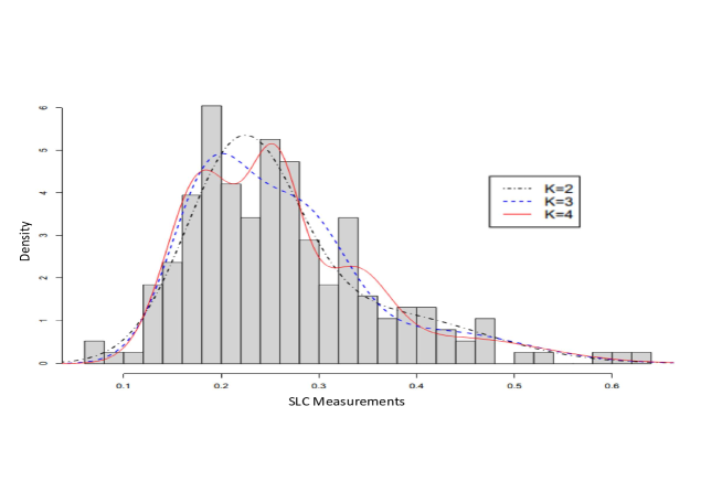
Figure 1: Histogram of 190 SLC measurements and estimated Gaussian mixture density curves.

We also conducted a Bayesian analysis on the SLD data using R package mixAK (komarek2014capabilities), where the Bayesian inference procedure on Gaussian mixture model with unknown number of components is discussed in richardson_bayesian_1997. We implement four different priors on $\tau$: uniform, Poisson(0.4), Poisson(1) and Poisson(5), all of which are truncated outside the set $\{1,\dots,10\}$. The priors used on $(\bm{\mu},\bm{\sigma})$ are the default priors (i.e., Gaussian and inverse Gamma priors) in mixAK. The posterior distributions for the four priors are plotted in Figure 2, with corresponding 95% credible sets $\{2,3\}$, $\{2\}$, $\{2,3\}$, $\{2,3,4\}$, respectively. It turns out the posterior distributions and their corresponding 95% credible sets of $\tau$ are quite different for different priors. Even in the cases with the same credible set, the posterior distributions are quite different. It is clear that the Bayesian inference of $\tau$ is very sensitive to the choice of the prior. A simulation study in Section 5.2 affirms this observation. The simulation study further suggests that the Bayesian procedure is not suited for the task of recovering the true $\tau_{0}$ (under repeated experiments) and its outcomes are also affected greatly by the default priors on $\bm{\mu}$ and $\bm{\sigma}$.

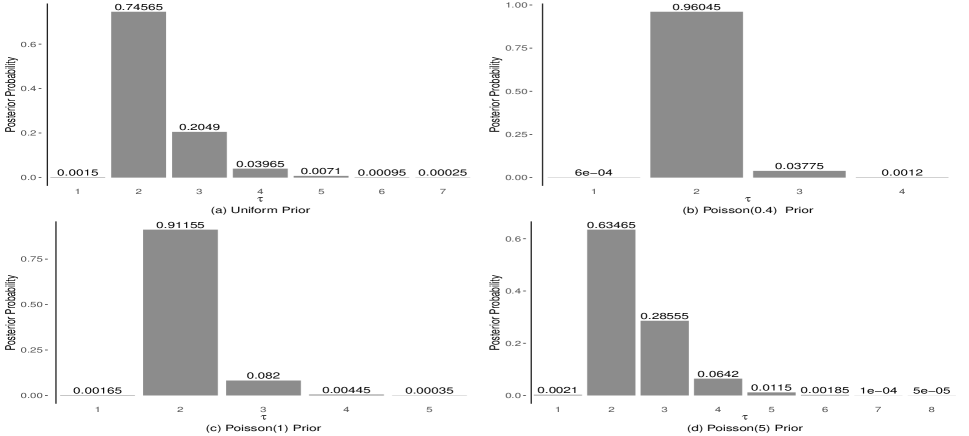
Figure 2: Posterior distributions of $\tau$ under four different priors: (a) uniform; (b) Poisson($\mu=0.4$); (c) Poisson($\mu=1$); (d) Poisson($\mu=5$); All priors are truncated outside the set $\{\tau:\tau=1,\dots,10\}$.

Reported in Table 2(a) are the corresponding estimated mean, standard deviation and weight of each component. We can also use the development of Section 4.3 to make inference for cluster mean $\mu_{k}^{(0)}$ and standard deviation $\sigma_{k}^{(0)}$, for $k=1,\ldots,\tau_{0}$. Reported in Table 2(b) are the level-$95\%$ representative intervals $(a_{k}^{*},b_{k}^{*})$ and $(q_{k}^{*},r_{k}^{*})$ of $\mu_{k}$ and $\sigma_{k}$, for $1\leq k\leq\tau$ and $\tau=2,3,4$, respectively. See Sections 3.3 and 4.3 for the definition of representative intervals. If $\tau_{0}$ is indeed one of the $\tau=2,3$ or $4$, then the representative intervals $(a_{k}^{*},b_{k}^{*})$ and $(q_{k}^{*},r_{k}^{*})$ of the corresponding row are level-$95\%$ confidence intervals for $\mu_{k}^{(0)}$ and $\sigma_{k}^{(0)}$, for $1\leq k\leq\tau_{0}$, respectively. However, we do not know which $\tau\in\Xi^{\prime}_{\alpha}(\bm{y}_{obs})=\{2,3,4\}$. To accommodate the uncertain in estimating $\tau_{0}$, we report instead that $90\%$ confidence sets of $(\tau_{0},\mu_{k}^{(0)})$ and $(\tau_{0},\sigma_{k}^{(0)})$, for a given $1\leq k\leq\tau_{0}$, are $\cup_{\tau^{*}\in\{2,3,4\}}\left(\{\tau^{*}\}\times(a_{k}^{*},b_{k}^{*})\right)$ and $\cup_{\tau^{*}\in\{2,3,4\}}\left(\{\tau^{*}\}\times(q_{k}^{*},r_{k}^{*})\right)$, respectively. This set of results provides a full picture on the uncertainty of the parameter estimations, across both the discrete parameter of the unknown number of components and the continuous location and scale parameters.

(a)
	Component Mean	Component SD	Weight
$\tau=2$	(0.2206,0.3654)	(0.0571,0.1012)	(0.7057,0.2943)
$\tau=3$	(0.1887,0.2809,0.4199)	(0.0414,0.0474,0.0886)	(0.4453,0.3866,0.168)
$\tau=4$	(0.1804,0.2556,0.3351,0.4403)	(0.0362,0.0268,0.0359,0.086)	(0.4018,0.2941,0.1742,0.1299)
(b)

	Confidence Intervals for $\mu_{k}^{(0)}$, $k=1,\ldots,\tau$	Confidence Intervals for $\sigma_{k}^{(0)}$, $k=1,\ldots,\tau$
$\tau=2$	(0.212, 0.258), (0.379, 0.495)	(0.055, 0.087), (0.019, 0.114)
$\tau=3$	(0.193, 0.245), (0.219, 0.439), (0.398, 0.463)	(0.0391, 0.075), (0.013, 0.321), (0.025, 0.078)
$\tau=4$	(0.168, 0.188), (0.212, 0.242), (0.321, 0.349), (0.404, 0.508)	(0.021, 0.062), (0.035, 0.053), (0.024, 0.063), (0.017, 0.161)

Table 2: Analysis of SLC data: (a) Estimated mean, standard deviation and weight of each component; (b) Corresponding level-$95\%$ representative intervals for $\mu_{k}$ and $\sigma_{k}$, $k=1,\ldots,\tau$. If $\tau_{0}$ is one of those in the level-$95\%$ confidence set of $\tau_{0}$ $\{2,3,4\}$, then the representative intervals in the corresponding row are level-$95\%$ confidence intervals for $\mu_{k}^{(0)}$ and $\sigma_{k}^{(0)}$, for $1\leq k\leq\tau_{0}$, respectively.

5.2 Simulation Study: Inference for $\tau_{0}$, $\mu_{j}^{(0)}$ and $\sigma_{j}^{(0)}$, $j=1,\ldots,\tau_{0}$

To further demonstrate the performance of our repro samples method, we carry out simulation studies in which the simulated Gaussian mixture data mimic the real SLC data. In particular, the true parameters of Gaussian mixture models used in our simulation studies are those in Table 2(a) with $\tau=3$ and $\tau=4$, respectively. In each setting of $\tau_{0}=3$ or $\tau_{0}=4$, we simulate $n=190$ data points using the corresponding parameters. For each simulated data, we apply the proposed repro samples method. The experiments are repeated 200 times in each setting.

The bar plots in Figure 3 summarize the 200 level-95% confidence sets of $\tau_{0}$ obtained using the proposed repro samples method for $\tau_{0}=3$ and $\tau_{0}=4$, respectively. It demonstrates good empirical performances of the proposed confidence set for $\tau_{0}$. Specifically, as shown in the plots, in both settings of $\tau_{0}=3$ and $\tau_{0}=4$, the proposed confidence set achieves the coverage rate of 99% and 96.5% respectively, both greater than 95%. Since the parameter space for $\tau_{0}$ is discrete, it is not always possible to achieve the exact level of 95%, and an over coverage is expected. In the study with $\tau_{0}=3,$ the average size of the proposed confidence set is about $3$, with a standard error of $0.05$. In Figure 3, we see our approach produces a confidence set of $\{2,3,4\}$ for the majority of the $200$ simulations. As for $\tau_{0}=4,$ more than 80% of the times, we get a confidence set of either $\{2,3,4\}$ or $\{2,3,4,5\}$, with the average size of the confidence set around $3.65$ and a standard error $0.05$.

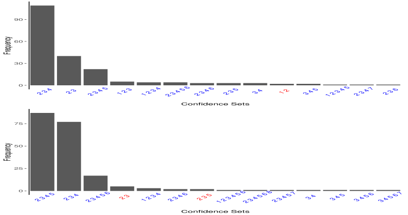
Figure 3: Bar plots of 200 level 95% repro samples confidence sets obtained in the simulation study (200 repetitions). The upper panel is for true $\tau_{0}=3$; lower for true $\tau_{0}=4.$

The simulation study can further demonstrate the importance of having a confidence set for $\tau_{0}$, as evidenced by the inferior performance of point estimations. For example, using the same simulated data, the classical BIC method recovers the true value of $\tau_{0}=3$ only 13 times (6.5%) out of the 200 repetitions. The number of times drops to $0$ (out of 200 repetitions) when the true $\tau_{0}=4.$ The results are not surprising, since with a strong penalty term the BIC point estimator is often biased towards smaller $\tau$ values in practice, even though the BIC estimator is known to be a consistent estimator. These two extremely low rates of correctly estimating the true $\tau_{0}$ highlight the challenge of the traditional point estimation method in our simulation examples, and more generally the risk of using just a point estimation in a Gaussian mixture model. Indeed, this result highlights the critical need to quantify the estimation uncertainty through a confidence set.

Additionally, we also illustrate the advantage of our proposed confidence set over the existing one-sided hypothesis testing approaches in roeder_graphical_1994 and chen_inference_2012, both of which advocate the use of the smallest $\tau_{0}$ that can not be rejected. We observe from our simulation study that such practices could very well mislead us to an overly small model, resulting in incorrect scientific interpretation. In particular, we find that, when the true $\tau_{0}=3$ and we perform the PLR test of chen_inference_2012 on $H_{0}:\tau_{0}=2$ versus $H_{1}:\tau_{0}=3$, only 74% times we fail to reject $H_{0}:\tau_{0}=2$. When the true $\tau_{0}=4$ and we perform the PLR test on $H_{0}:\tau_{0}=3$ versus $H_{1}:\tau_{0}=4$, we fail 93% times to reject $H_{0}:\tau_{0}=3$. These results suggest that most of the time, the PLR test prefers a wrong $\tau$ over the true one. Furthermore, inverting either of the one-sided tests does not produce an as useful confidence set, since the upper bound of the set is $\infty$. In conclusion, the proposed confidence set by the repro samples method is a more intact approach to conducting inference on $\tau_{0}$ compared to the one that uses only a hypothesis testing method.

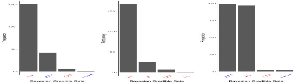
(a)                                          (b)                                           (c)

Figure 4: Bar plots of the 200 95% Bayesian credible sets obtained in the simulation study (200 repetitions) with $\tau_{0}=4$. Prior choices are (a) uniform; (b) Poisson($\mu=1$); (c) Poisson($\mu=5$); All priors truncated over $\{\tau=1,\dots,10\}$.

We further compare the performance of the Bayesian procedure described in richardson_bayesian_1997 when the number of components is unknown. The data used are the same as those in Figure 3 with $\tau_{0}=4$. Figure 4 summarizes the results from the Bayesian procedure by R package mixAK. Here, we display the credible sets produced using (a) uniform prior on $\tau=1,\dots,10$; (b) Poisson(1) prior, which prefers smaller $\tau$; and (c) Poisson(5) prior, whose mode is $4$ and matches with the true $\tau_{0}$. We see that the Bayesian level-$95\%$ credible sets consistently underestimate and fail to cover $\tau_{0}$, with the coverage rate equal to 21.5%, $0\%$ and $50.5\%$, respectively. In addition, the outcomes of the Bayesian procedure are sensitive to the specification of the prior distribution of $\tau,$ as evidenced by the drastic differences among the three panels of Figure 4.

At first glance, the underestimation of $\tau_{0}$ observed in Figure 4(a) with the uniform prior is somewhat surprising. However, further investigation reveals that the priors on $\bm{\mu}$ and $\bm{\sigma}$ also have a significant impact on estimating $\tau$, and the underestimation is attributable to the shrinkage effect of implementing a multilevel hierarchical model (richardson_bayesian_1997). Indeed, it is well known that shrinkage is ubiquitous when parameters are modeled hierarchically. Here both the means and variances of the components would share a common prior, thus over-promoting smaller $\tau$ as observed across all three plots in Figure 4.

Finally, we use the same $200$ simulated data sets with $\tau_{0}=3$ and $4$, respectively, to evaluate the performance of the confidence sets for $\mu_{j}^{(0)}$ and $\sigma_{j}^{(0)}$, $j=1,\ldots,\tau_{0}$, using the method described in Section 4.3. Table 3 reports the coverage rates and average widths of these confidence sets, where the values in the brackets are the corresponding standard errors. When $\tau_{0}=3,$ the proposed confidence sets have a high coverage rate across the board. When $\tau_{0}=4$, the coverages for $\sigma_{j}^{(0)}$’s still meet or exceed the 95% confidence level for three of all four clusters, with the coverage for the remaining cluster 92.5%. As for $\mu_{j}^{(0)}$’s, two clusters seem to slightly undercover at 91.0% and 92.5%, respectively. The undercover might be because more overlapping between the clusters complicates the computation of the candidate set. Another contributing factor might be the smaller sample size of each cluster compared to when $\tau_{0}=3$, which leads to greater volatility in the resulting confidence sets. Regardless, these results indicate that the proposed robust confidence sets generally achieve desired coverage rates for both $\mu^{(0)}$’s and $\sigma^{(0)}$’s. To the best of our knowledge (in private communications), this set of empirical coverage rates on means and variances (even if $\tau_{0}$ is given) are among the best in simulation studies mimicking the SLC data.

		Coverage	Average Width (SD)
$\tau_{0}=3$	$\mu_{j}^{(0)}$	.985, .965, .975	.136(.004), .202(.006), .330(.004)
	$\sigma_{j}^{(0)}$	.995, .985, .995	.029(.002), .010(.006), .042(.003)
$\tau_{0}=4$	$\mu_{j}^{(0)}$	.910, .926, .940, .955	.100(.004), .192(.008), .256(.011), .215(.006)
	$\sigma_{j}^{(0)}$	.950, .925, .965, .960	.015(.002), .060(.005), .076(.008), .048(.004)

Table 3: Simulation Results: Coverage and average width of $\mu_{j}^{(0)}$ and $\sigma_{j}^{(0)}$, $j=1,\ldots,\tau_{0}$, $\tau_{0}=3$ and $4$; SD is for standard deviation; Repetitions is $200$.

In summary, the inference problems in the Gaussian mixture model are ‘highly nontrivial’, as stated in wasserman2020universal. Existing methods, including the point estimation, hypothesis testing methods, and Bayesian procedures that we compared, all predominantly miss the true $\tau_{0}$, with outcomes frequently biased toward smaller $\tau$ values. Furthermore, the credible sets by the Bayesian method do not have frequentist coverage rates and they are also very sensitive to the choices of priors on $\tau$, $\bm{\mu}$, and $\bm{\sigma}$. The proposed repro samples method, on the contrary, provides valid confidence sets with desirable coverage rates. It is also the only method that gives us a two-sided confidence set for $\tau_{0}$ with guaranteed performance. It can effectively quantify uncertainty and makes inferences for both the discrete $\tau_{0}$ and the continuous $\bm{\mu}_{j}^{(0)}$ and $\bm{\sigma}_{j}^{(0)}$, $j=1,\ldots,\tau_{0}$.

6 Nuclear mapping by a test statistic and connection to classical Neyman-Pearson method

In a classical Neyman-Pearson testing problem $H_{0}:\mathop{\theta\kern-4.49997pt\hbox{$\theta$}}\nolimits_{0}=\mathop{\theta\kern-4.49997pt\hbox{$\theta$}}\nolimits$ versus $H_{1}:\mathop{\theta\kern-4.49997pt\hbox{$\theta$}}\nolimits_{0}\not=\mathop{\theta\kern-4.49997pt\hbox{$\theta$}}\nolimits$, we often construct a test statistic, say $\widetilde{T}(\bm{y}_{obs},\mathop{\theta\kern-4.49997pt\hbox{$\theta$}}\nolimits)$, and assume that we know the distribution of $\widetilde{T}(\bm{Y},\mathop{\theta\kern-4.49997pt\hbox{$\theta$}}\nolimits)$ for $\bm{Y}=G(\mathop{\theta\kern-4.49997pt\hbox{$\theta$}}\nolimits,\bm{U})$ generated under $H_{0}:\mathop{\theta\kern-4.49997pt\hbox{$\theta$}}\nolimits_{0}=\mathop{\theta\kern-4.49997pt\hbox{$\theta$}}\nolimits$. Under the classical framework, we can derive a level-$\alpha$ acceptance region $A_{\alpha}(\mathop{\theta\kern-4.49997pt\hbox{$\theta$}}\nolimits)=\big{\{}\bm{y}_{obs}\big{|}\widetilde{T}(\bm{y}_{obs},\mathop{\theta\kern-4.49997pt\hbox{$\theta$}}\nolimits)\in B_{\alpha}(\mathop{\theta\kern-4.49997pt\hbox{$\theta$}}\nolimits)\big{\}}$, where the set $B_{\alpha}(\mathop{\theta\kern-4.49997pt\hbox{$\theta$}}\nolimits)$ satisfies $\mathbb{P}\big{\{}\widetilde{T}(\bm{Y},\mathop{\theta\kern-4.49997pt\hbox{$\theta$}}\nolimits)\in B_{\alpha}(\mathop{\theta\kern-4.49997pt\hbox{$\theta$}}\nolimits)\big{\}}\geq\alpha$. Then, by the property of test duality (i.e., the so-called Neyman Inversion method), a level-$\alpha$ confidence set is

$$\widetilde{\Gamma}_{\alpha}(\bm{y}_{obs})=\left\{\mathop{\theta\kern-4.49997pt\hbox{$\theta$}}\nolimits:\bm{y}_{obs}\in A_{\alpha}(\mathop{\theta\kern-4.49997pt\hbox{$\theta$}}\nolimits)\right\}=\left\{\mathop{\theta\kern-4.49997pt\hbox{$\theta$}}\nolimits:\widetilde{T}(\bm{y}_{obs},\mathop{\theta\kern-4.49997pt\hbox{$\theta$}}\nolimits)\in B_{\alpha}(\mathop{\theta\kern-4.49997pt\hbox{$\theta$}}\nolimits)\right\}.$$

Now suppose our nuclear mapping $T(\bm{u},\mathop{\theta\kern-4.49997pt\hbox{$\theta$}}\nolimits)$ for a potential $\mathop{\theta\kern-4.49997pt\hbox{$\theta$}}\nolimits$ is defined through this test statistic by the formula below:

$$T(\bm{U},\mathop{\theta\kern-4.49997pt\hbox{$\theta$}}\nolimits)=\widetilde{T}(\bm{Y},\mathop{\theta\kern-4.49997pt\hbox{$\theta$}}\nolimits)=\widetilde{T}(G({\mathop{\theta\kern-4.49997pt\hbox{$\theta$}}\nolimits},\bm{U}),\mathop{\theta\kern-4.49997pt\hbox{$\theta$}}\nolimits),$$ (31)

where $\bm{Y}=G(\mathop{\theta\kern-4.49997pt\hbox{$\theta$}}\nolimits,\bm{U})$ using the same $\mathop{\theta\kern-4.49997pt\hbox{$\theta$}}\nolimits$. Since $\mathbb{P}\left\{T(\bm{U},\mathop{\theta\kern-4.49997pt\hbox{$\theta$}}\nolimits)\in B_{\alpha}(\mathop{\theta\kern-4.49997pt\hbox{$\theta$}}\nolimits)\right\}=\mathbb{P}\big{\{}\widetilde{T}(\bm{Y},\mathop{\theta\kern-4.49997pt\hbox{$\theta$}}\nolimits)\in B_{\alpha}(\mathop{\theta\kern-4.49997pt\hbox{$\theta$}}\nolimits)\big{\}}$ $\geq\alpha$ for the same $B_{\alpha}(\cdot)$, a level-$\alpha$ confidence set of (4) by the repro samples method is

$$\Gamma_{\alpha}(\bm{y}_{obs})=\left\{\mathop{\theta\kern-4.49997pt\hbox{$\theta$}}\nolimits:\exists\bm{u}^{*}\in{\cal U}\mbox{ s.t. }\bm{y}_{obs}=G({\mathop{\theta\kern-4.49997pt\hbox{$\theta$}}\nolimits},\bm{u}^{*}),\widetilde{T}(G({\mathop{\theta\kern-4.49997pt\hbox{$\theta$}}\nolimits},\bm{u}^{*}),\mathop{\theta\kern-4.49997pt\hbox{$\theta$}}\nolimits)\in B_{\alpha}(\mathop{\theta\kern-4.49997pt\hbox{$\theta$}}\nolimits)\right\}.$$

Lemma 4 below suggests that this $\Gamma_{\alpha}(\bm{y}_{obs})$ is always smaller than or equal to the confidence set $\widetilde{\Gamma}_{\alpha}(\bm{y}_{obs})$ by the Neyman method; i.e., $\Gamma_{\alpha}(\bm{y}_{obs})\subseteq\widetilde{\Gamma}_{\alpha}(\bm{y}_{obs})$. See Appendix A for a proof.

Lemma 4.

If the nuclear mapping function is defined through a test statistic as in (31), then we have $\Gamma_{\alpha}(\bm{y}_{obs})\subseteq\widetilde{\Gamma}_{\alpha}(\bm{y}_{obs})$. The two sets are equal $\Gamma_{\alpha}(\bm{y}_{obs})=\widetilde{\Gamma}_{\alpha}(\bm{y}_{obs})$, when $\widetilde{\Gamma}_{\alpha}(\bm{y}_{obs})\subseteq\big{\{}\mathop{\theta\kern-4.49997pt\hbox{$\theta$}}\nolimits:\bm{y}_{obs}=G({\mathop{\theta\kern-4.49997pt\hbox{$\theta$}}\nolimits},\bm{u}^{*}),\exists\,\bm{u}^{*}\in{\cal U}\big{\}}$.

We note that it is possible that $\Gamma_{\alpha}(\bm{y}_{obs})$ is strictly smaller than $\widetilde{\Gamma}_{\alpha}(\bm{y}_{obs})$; i.e., $\Gamma_{\alpha}(\bm{y}_{obs})\subsetneq\widetilde{\Gamma}_{\alpha}(\bm{y}_{obs})$. The following is such an example where $\Gamma_{\alpha}(\bm{y}_{obs})$ is strictly smaller than $\widetilde{\Gamma}_{\alpha}(\bm{y}_{obs})$.

 Example 2.

Suppose $\bm{y}_{obs}=(y_{1},\ldots,y_{n})^{\top}$ is a set of samples from the model

$$Y_{i}=\theta_{0}+U_{i},\qquad U_{i}\sim U(-1,1),\quad i=1,\ldots,n.$$

Here, $\Theta=(-\infty,+\infty)$, ${\cal Y}=(-\infty,\infty)$. An unbiased point (and also $\sqrt{n}$-consistent) estimator is $\bar{Y}=\frac{1}{n}\sum_{i=1}^{n}Y_{i}$. Suppose we use the test statistic $\widetilde{T}(\bm{y}_{obs},\theta)=$ $\bar{y}-\theta$. Since $n\{(\bar{Y}-\theta)$ $+1\}/2=\sum_{i=1}^{n}\frac{U_{i}+1}{2}$ follows an Irwin-Hall distribution when $\theta$ is the true value $\theta_{0}$, by the classical testing method a level-$95\%$ confidence interval is $\widetilde{\Gamma}_{.95}(\bm{y}_{obs})=(\bar{y}-\frac{2}{n}q_{.975}+1,\bar{y}+\frac{2}{n}q_{.975}-1)$. Here, $q_{.975}$ is the $97.5\%$ quantile of the Irwin-Hall distribution. If we use our repro samples method, our confidence set is then $\Gamma_{.95}(\bm{y}_{obs})=\big{\{}\theta:y_{i}=\theta+u_{i}^{*},i=1,\ldots,n;\,\bar{y}\in(\theta-\frac{2}{n}q_{.975}+1,\theta+\frac{2}{n}q_{.975}-1);\exists\bm{u}^{*}\in(-1,1)^{n}\big{\}}=\left\{\theta:\theta\in\cap_{i=1}^{n}(y_{i}-1,y_{i}+1)\right\}\cap\widetilde{\Gamma}_{.95}(\bm{y}_{obs})$. Since the constraint $\{\theta\in\cap_{i=1}^{n}(y_{i}-1,y_{i}+1)\}$ is often in tack, the strictly smaller statement $\Gamma(\bm{y}_{obs})\subsetneq\widetilde{\Gamma}(\bm{y}_{obs})$ holds for many realizations of $\bm{y}_{obs}$.

As an illustration, consider the case $\theta=0$ and $n=3$, in which $q_{.975}=2.4687$. Suppose we have a sample realization $\bm{y}_{obs}=(-0.430,0.049,0.371)^{\top}$. By a direct calculation, $\widetilde{\Gamma}_{\alpha}(\bm{y}_{obs})=(-.6458,.6458)$ and $\Gamma_{\alpha}(\bm{y}_{obs})=\big{\{}\mathop{\theta\kern-4.49997pt\hbox{$\theta$}}\nolimits:y_{obs,i}=\theta+u_{i}^{*},i=1,2,3;\,\exists(u_{1}^{*},u_{2}^{*},u_{3}^{*})\in(-1,1)\times(-1,1)\times(-1,1)\big{\}}\cap\widetilde{\Gamma}_{\alpha}(\bm{y}_{obs})=\big{\{}(-1.430,.570)\cap(-.951,1.049)\cap(-.629,1.371)\big{\}}\cap(-.6458,.6458)=(-.629,.570)$. Clearly, $\Gamma_{\alpha}(\bm{y}_{obs})\subsetneq\widetilde{\Gamma}_{\alpha}(\bm{y}_{obs})$. We repeated the experiment $1,000$ times. The coverage rates of $\widetilde{\Gamma}_{\alpha}(\bm{y}_{obs})$ and $\Gamma_{\alpha}(\bm{y}_{obs})$ are both $95.1\%$. Among the $1,000$ repetitions, $219$ times $\Gamma_{\alpha}(\bm{y}_{obs})=\widetilde{\Gamma}_{\alpha}(\bm{y}_{obs})$ and $781$ times $\Gamma_{\alpha}(\bm{y}_{obs})\subsetneq\widetilde{\Gamma}_{\alpha}(\bm{y}_{obs})$. The average lengths of $\Gamma_{\alpha}(\bm{y}_{obs})$ and $\widetilde{\Gamma}_{\alpha}(\bm{y}_{obs})$ are $0.915$ and $1.292$, respectively.

We note that a nuclear mapping function does not need to be a test statistic, but if it is defined through a test statistics as in (31) then there are immediate implications. First, the confidence set $\Gamma(\bm{y}_{obs})$ by the repro samples method is more desirable, since by Lemma 4 $\Gamma(\bm{y}_{obs})$ is either smaller or the same as the one obtained by the classical testing approach. Second, if the test statistic is optimal (in the sense that it leads to a powerful test), then $\Gamma(\bm{y}_{obs})$ constructed by the corresponding nuclear mapping defined as in (31) is also optimal. We have a formal statement in Corollary 4 below, where a level-$\alpha$ uniformly most accurate (UMA) confidence set (also called Neyman shortest) refers to a level-$\alpha$ confidence set that minimizes the probability of false coverage (i.e., probability of covering a wrong parameter value) over a class of level-$\alpha$ confidence sets; cf., tCAS90a. A proof of the corollary is provided in Appendix A.

Corollary 4.

(a) If the test statistic $\widetilde{T}(\bm{y}_{obs},\mathop{\theta\kern-4.49997pt\hbox{$\theta$}}\nolimits)$ corresponds to the uniformly most powerful test and $\widetilde{\Gamma}(\bm{y}_{obs})$ is a level-$\alpha$ UMA confidence set, then the set $\Gamma(\bm{y}_{obs})$ by the corresponding repro sample method is also a level-$\alpha$ UMA confidence set.
(b) If the test statistic $\widetilde{T}(\bm{y}_{obs},\mathop{\theta\kern-4.49997pt\hbox{$\theta$}}\nolimits)$ corresponds to the uniformly most powerful unbiased test and $\widetilde{\Gamma}(\bm{y}_{obs})$ is a level-$\alpha$ UMA unbiased confidence set, then the confidence set $\Gamma(\bm{y}_{obs})$ by the corresponding repro sample method is also a level-$\alpha$ UMA unbiased confidence set.

We note that the repro samples method is more general and flexible than the often-recommended likelihood inference approach. Typical hypothesis testing framework often involves finding a pivotal quantity and its distribution, and the most commonly used pivotal quantity is perhaps the likelihood ratio test statistics (LRT) (cf., Reid2015). It is well known that the negative two log-LRT statistic is asymptotically $\chi^{2}$-distributed and a test developed based on the LRT statistic is asymptotically efficient (tCAS90a, p381) under some regularity conditions. When these regularity conditions hold, one can define the nuclear mapping function through the LRT statistic and our repro samples method enjoys the same large sample optimality. When these regularity conditions do not hold and the chi-square approximation fails, the repro samples method can achieve improved performance over the LRT-based inference, even though by the Neyman-Pearson Lemma the LRT is uniformly most powerful for a simple-versus-simple test. Below is one such example.

 Example 3 (Likelihood inference; Example 2 continues).

The likelihood function under the setting of Example 2 is $L(\theta|\bm{y}^{obs})=\prod\nolimits_{i=1}^{n}\big{[}I\{-1<y_{i}-\theta\leq 1\}/2\big{]}\propto I\big{\{}\max\nolimits_{1\leq i\leq n}|y_{i}-\theta|<1\big{\}}.$. The LRT statistic for test $H_{0}:\mathop{\theta\kern-4.49997pt\hbox{$\theta$}}\nolimits_{0}=\mathop{\theta\kern-4.49997pt\hbox{$\theta$}}\nolimits$ vs $H_{1}:\mathop{\theta\kern-4.49997pt\hbox{$\theta$}}\nolimits_{0}\not=\mathop{\theta\kern-4.49997pt\hbox{$\theta$}}\nolimits$ is $\lambda_{\theta}(\bm{y}_{obs})=I\big{\{}\max\nolimits_{1\leq i\leq n}|y_{i}-\theta|<1\big{\}}$, but $-2\log\{\lambda_{\theta}(\bm{Y})\}$ does not converge to a $\chi^{2}$ distribution. Since $\lambda_{\theta}(\bm{y}_{obs})$ is decreasing in $\widetilde{T}(\bm{y}_{obs},\theta)=\max\nolimits_{1\leq i\leq n}|y_{i}-\theta|$, the LRT rejects $H_{0}$ with a large $\widetilde{T}(\bm{y}_{obs},\theta)$, which leads to a level-$\alpha$ confidence set

$$\widetilde{\Gamma}_{\alpha}(\bm{y}_{obs})=\{\theta:\max\nolimits_{1\leq i\leq n}|y_{i}-\theta|<\alpha^{1/n}\}=(y_{(n)}-\alpha^{1/n},y_{(1)}+\alpha^{1/n}).$$

We get the same confidence set if we directly define our nuclear mapping function through $\widetilde{T}(\bm{y}_{obs},\theta)=\max\nolimits_{1\leq i\leq n}|y_{i}-\theta|$. Alternatively, we consider another choice of a vector nuclear mapping function $T(\bm{u},\theta)=(u_{(1)},u_{(n)})$, where $u_{(k)}$ is the $k$th order statistic of a sample from $U(-1,1)$. Let $c_{\alpha}\in(0,1)$ be a solution of $({c_{\alpha}+1})^{n}-2^{n-1}c_{\alpha}^{n}=2^{n-1}{(1-\alpha)}$. We can show $\mathbb{P}\{(U_{(1)},U_{(n)})\in B_{\alpha}\}=\alpha$ for $B_{\alpha}=(-1,-c_{\alpha})\times(c_{\alpha},1)$. Thus, a level-$\alpha$ confidence set is $\Gamma_{\alpha}(\bm{y}_{obs})$ $=\{\theta:y_{(n)}-1<\theta<y_{(1)}+1;y_{(1)}-\theta<-c_{\alpha},y_{(n)}-\theta>c_{\alpha}\},$ which is simplified to

$$\Gamma_{\alpha}(\bm{y}_{obs})=\big{(}\max\big{\{}y_{(1)}+c_{\alpha},y_{(n)}-1\big{\}},\min\big{\{}y_{(n)}-c_{\alpha},y_{(1)}+1\big{\}}\big{)}.$$

Note that, if we consider the space of $(U_{(1)},U_{(n)})$, the Borel set for the LRT confidence set $\widetilde{\Gamma}_{\alpha}(\bm{y}_{obs})$ is $\tilde{B}_{\alpha}=(-\alpha^{1/n},\alpha^{1/n})\times(-\alpha^{1/n},\alpha^{1/n})$, which is much bigger than the Borel set $B_{\alpha}=(-1,-c_{\alpha})\times(c_{\alpha},1)$ of the alternative method.

We have conducted a numerical study with true $\theta_{0}=0$ and $n=5,20,200$, respectively. In all cases, the coverage rates of both confidence intervals are right on target around $95\%$ in 3000 repetitions. The intervals by the repro sample method are on average consistently shorter than those obtained using the LRT method across all sample sizes, as evidenced in Figure 5. Although a LRT is uniformly most powerful for a simple-versus-simple test by the Neyman-Pearson Lemma, it is not the case for the two-sided test in this example. Here, we can explore and use the repro samples method to obtain a better confidence interval.

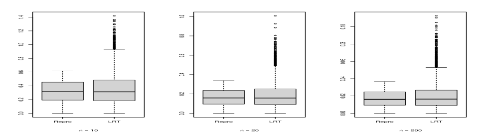
Figure 5: Side-by-side box plots comparing the widths of the two 95% confidence intervals discussed in Example 4, for $n=10,20$ and $200$, respectively; The number of repetitions $=5000$. The empirical coverage rates are $(.952,.954,.949)$ for the repro method and $(.950,.952,.950)$ for the LRT method, respectively, all on the target. The average interval lengths are $(.320,.166,.017)$, respectively, for the repro method, all smaller than the corresponding lengths $(.351,.184,.020)$ for the LRT method.

Finally, we emphasize that the nuclear mapping function $T(\bm{u},\mathop{\theta\kern-4.49997pt\hbox{$\theta$}}\nolimits)$ does not need to be a test statistic since it is not necessarily a function of data $\bm{y}^{\prime}=G(\mathop{\theta\kern-4.49997pt\hbox{$\theta$}}\nolimits,\bm{u})$. Allowing the nuclear mapping to be a function of $\bm{u}$ provides more flexibility for developing inference procedures than the conventional testing approach. For example, consider a simple $\text{Bernoulli}(\theta)$ model with a single observation $y_{obs}$ generated by $Y=I(U<\theta_{0})$, $U\sim\text{Uniform}(0,1).$ To get a confidence set for $\theta_{0}$, we can let $T(u,\theta)=u$, and define

$$B_{\alpha}(\theta)=\begin{cases}[1-\alpha,1]&\theta>0.5\\ [\frac{1-\alpha}{2},\frac{1+\alpha}{2}]&\theta=0.5\\ [0,\alpha]&\theta<0.5\end{cases}.$$

Then, following (4), we construct the repro samples confidence set by $\Gamma_{\alpha}(y_{obs})=[1-\alpha,1]{\bf 1}_{\{y_{obs}=1\}}+[0,\alpha]{\bf 1}_{\{y_{obs}=0\}}$. Apparently, $U$ is not a function of $Y$, since it is impossible to solve for $U$ in the structure equation $Y=I(U<\theta)$ when given $(Y,\theta)$. Thus, $T(U,\theta)=U$ is not a test statistic. A more complex example is in ChandraWorking1 in which the authors use the repro samples method (with a nuclear mapping function that cannot be expressed as a test statistic) to obtain confidence intervals for the ranks of $78$ Veterans Health Administration Hospitals in the US.

7 Concluding remarks and future research

This paper develops a repro samples method to provide an innovative, flexible, and efficient framework for making inferences for a broad range of problems, including many previously challenging open problems. The proposed framework utilizes (explicitly or implicitly) artificially generated samples that mimic the observed data to quantify inference uncertainty, and we provide both finite and approximate (large sample) theories to support the framework. Further developments and discussions cover topics such as the effective handling of nuisance parameters, the use of a data-driven candidate set to enhance computing efficiency, and examining the relationship and advantages over the classical hypothesis testing procedures, along with the associated optimality results. To construct the confidence sets, in many cases, the repro samples method provides explicit mathematical solutions, while in other scenarios, it employs Monte-Carlo approaches to attain numerical solutions. A notable strength of the repro samples framework is that it does not rely on the likelihood or large sample CLT for inference developments. Furthermore, the framework is flexible, making it particularly effective for a diverse set of challenging inference problems, including those irregular problems that involve discrete or non-numerical inference targets.

The article also includes a case study example of Gaussian mixture models to demonstrate the use of the repro samples procedure. The classic Gaussian mixture models have a long history and are prevalent in statistics and data science. Although the models may appear simple, the associated inference problems are highly non-trivial and challenging, particularly when the number of components is unknown. This is because it involves a mixed type (discrete and continuous) of unknown parameters, many of which have varying lengths. In the case study example, we provide a comprehensive solution for the long-standing, important, yet still open inference problems using the repro samples method. Theoretical derivations specifically tailored to the Gaussian mixture models are provided. Moreover, numerical studies in a real-data setting and comparisons with existing approaches demonstrate that the repro samples method is the only effective approach that can consistently cover model parameters (both discrete and continuous types) with the desired coverage rates. Another example of addressing open challenging problems is demonstrated in wang2022highdimenional, in which the authors provide the first comprehensive method to incorporate model selection uncertainty in inference problems for high dimensional linear models. In particular, the authors have developed confidence sets for the unknown true (sparse) model, the regression coefficients, or jointly for both the true model and the coefficients with guaranteed finite-sample performances, providing a full picture of inference uncertainties covering model space, regression coefficients, and more.

Indeed, by considering broad types of parameters and models, the repro samples method significantly extends the scope and reach of statistical inference. Besides the two classical case study examples mentioned in the previous paragraph, The repro samples method can also be used to provide interpretable inference for many complex black-box machine learning models. For instance, it can be used in a tree model to provide a confidence set for the underlying ‘true’ tree model that generates observed data, and using the confidence tree set to develop a principled random forest (that only ensemble trees in a confidence set). Preliminary results have demonstrated both theoretical and numerical advantages over the regular ensemble tree methods (e.g., the standard random forest method, etc.). The repro samples method can further be used to construct a confidence set for the architecture parameters (layer and vertices) of the smallest neural network model(s) that can generate observed data. Due to space limitation, these results will be reported in separate research papers. Finally, the data $\bm{y}^{obs}$ mentioned in this paper can also be non-numerical (e.g., graphical network data; voice data; image data; etc). In this case, we can still apply the repro sample method to make inference for such data, as long as we still have a generative model and a metric to measure certain conformity among the non-numerical data. This is also a future research direction. We anticipate that the repro samples method can potentially serve as a stepping stone for establishing theoretical foundations in data science and for providing informed statistical inference and prediction in many machine learning problems.

The assumed algorithmic model (1) or its extension (8) encompass most models assumed in the current literature. Nevertheless, it is still of interest to investigate the impact if the assumed model (1) or (8) is misspecified; for example, the distribution of $\bm{U}$ is unknown or the form $G(\cdot)$ is misspecified. We first note that, in some cases, it is possible to estimate the distribution of $\bm{U}$. For instance, in the high dimensional sparse linear model studies in wang2022highdimenional,it is possible to use their model candidate set to get a supper model, use the super model to get residuals, and then use the residuals to estimate the distribution of $\bm{U}$. Alternatively, instead of assuming Gaussian errors in the linear model, we can also assume the error distribution is from a more general family, i.e., $\propto e^{-|u_{i}|^{\eta_{1}}/\eta_{2}}$, and then estimate the additional parameters $\eta_{1}>0$ and $\eta_{2}>0$ together with other model parameters. In cases when the form of $G(\cdot,\cdot)$ is unknown, the target parameter can perhaps be defined as the parameter in the misspecified model family that is closest to the true model that generated the observed data. Relevant research at this front includes model calibration (e.g., smith2007calibration) and variational Bayes (e.g., wang2019variational). Similar to all model-based approaches, model robustness against misspecification is an important research topic here as well. It is certainly an interesting future topic to be further investigated.

Finally, most of our theoretical developments are centered on showing the validity of the approaches. Section 6 shows that the repro samples development subsumes the classical Neyman procedure in the sense that a confidence set obtained by our repro samples method is always better than (either the same as or smaller than) that obtained by inverting the Neyman test procedure. If a confidence set obtained by the classical Neyman procedure is optimal, our repro samples method can also get the same optimal set. Furthermore, the repro samples development borrows the inversion idea that is deeply rooted in a fiducial method, and such an inversion method does not lose any information and often enjoys “good finite-sample performance” (Hannig2016). Nevertheless, the choice of the nuclear mapping function and its associated are problem specific and have impact on the size of confidence sets. Further research on these efficiency issues is also an interesting research topic. Due to space limitations, we will carry out the research in a separate paper.

Appendix A: Theoretical Proofs

A-I. Proofs of Theoretical Results in Section 2

Proof of Theorem 1.

Since $\bm{y}_{obs}=G({\mathop{\theta\kern-4.49997pt\hbox{$\theta$}}\nolimits}_{0},{\bm{u}}^{rel})$ always holds, if $T({\bf u}^{rel},\mathop{\theta\kern-4.49997pt\hbox{$\theta$}}\nolimits_{0})\in B_{\alpha}(\mathop{\theta\kern-4.49997pt\hbox{$\theta$}}\nolimits_{0})$, then $\mathop{\theta\kern-4.49997pt\hbox{$\theta$}}\nolimits_{0}\in\Gamma_{\alpha}(\bm{y}_{obs})\not=\emptyset$. That is, $\{\mathop{\theta\kern-4.49997pt\hbox{$\theta$}}\nolimits_{0}\in\Gamma_{\alpha}(\bm{y}_{obs})\}\supseteq\{T({\bf u}^{rel},\mathop{\theta\kern-4.49997pt\hbox{$\theta$}}\nolimits_{0})\in B_{\alpha}(\mathop{\theta\kern-4.49997pt\hbox{$\theta$}}\nolimits_{0})\}$. Similarly, for the random version $\bm{Y}=$ $G({\mathop{\theta\kern-4.49997pt\hbox{$\theta$}}\nolimits}_{0},{\bf U})$, we have $\left\{\mathop{\theta\kern-4.49997pt\hbox{$\theta$}}\nolimits_{0}\in\Gamma_{\alpha}({\bm{Y}})\right\}\supseteq\left\{T({\bf U},\bm{\theta}_{0})\in B_{\alpha}(\bm{\theta}_{0})\right\}$. Thus, $\mathbb{P}\{\mathop{\theta\kern-4.49997pt\hbox{$\theta$}}\nolimits_{0}\in\Gamma_{\alpha}(\bm{Y})\}\geq\mathbb{P}\{T(\bm{U},\mathop{\theta\kern-4.49997pt\hbox{$\theta$}}\nolimits_{0})\in B_{\alpha}(\mathop{\theta\kern-4.49997pt\hbox{$\theta$}}\nolimits_{0})\}\geq\alpha$, where the last equation is by (3). The same proof applies in the situation when (3) holds approximately. ∎

Proof of Corollary 1.

Under $H_{0}$, we have $\bm{\theta}_{0}\in\Theta_{0}$ and thus

$$\mathbb{P}\{p(\bm{Y})\leq\gamma\}\leq\mathbb{P}\left[\inf\left\{\alpha^{\prime}:\bm{\theta}_{0}\in\Gamma_{\alpha^{\prime}}(\bm{Y})\right\}\geq 1-\gamma\right]=\mathbb{P}\left\{\bm{\theta}_{0}\not\in\Gamma_{\alpha^{\prime}}(\bm{Y}),\forall\,\alpha^{\prime}<1-\gamma\right\}\leq\gamma,$$

for any significance level $\gamma.$ Thus, the Type I error is controlled. ∎

Proof of Theorem 2.

The proof is similar to that of Theorem 1. Specifically, since $g(\bm{Y},\mathop{\theta\kern-4.49997pt\hbox{$\theta$}}\nolimits,$ $\bm{U})$ $=0$ holds for $\bm{\theta}=\bm{\theta}_{0}$, we have $\big{\{}\mathop{\theta\kern-4.49997pt\hbox{$\theta$}}\nolimits_{0}\in\Gamma_{\alpha}({\bm{Y}})\big{\}}\subseteq\big{\{}T({\bf U},\bm{\theta}_{0})\in B_{\alpha}(\bm{\theta}_{0})\big{\}}$ for the set $\Gamma_{\alpha}({\bm{Y}})$ defined in (9). Thus, Theorem 2 follows from $\mathbb{P}\{\mathop{\theta\kern-4.49997pt\hbox{$\theta$}}\nolimits_{0}\in\Gamma_{\alpha}(\bm{Y})\}\geq\mathbb{P}\{T(\bm{U},\mathop{\theta\kern-4.49997pt\hbox{$\theta$}}\nolimits_{0})\in B_{\alpha}(\mathop{\theta\kern-4.49997pt\hbox{$\theta$}}\nolimits_{0})\}\geq\alpha,$ where the last inequality is by (3). The same proof applies in the situation when (3) holds approximately.

∎

A-II. Proofs of Theoretical Results in Section 3

Proof of Lemma 1.

It follows from the definitions in (11) and (12) that $\mathbb{P}\left\{T_{p}(\bm{U},\mathop{\theta\kern-4.49997pt\hbox{$\theta$}}\nolimits)\leq\alpha\right\}\geq\mathbb{P}\left\{\nu(\bm{U},\eta,\bm{\beta},\bm{\beta})\ \leq\alpha\right\}\geq\mathbb{P}\{\mathop{\theta\kern-4.49997pt\hbox{$\theta$}}\nolimits\in\Gamma_{\alpha}(G(\bm{U},\mathop{\theta\kern-4.49997pt\hbox{$\theta$}}\nolimits))\}\geq\alpha,$ where $\Gamma_{\alpha}(G(\bm{u},\mathop{\theta\kern-4.49997pt\hbox{$\theta$}}\nolimits))$ is that used in (11). ∎

Proof of Theorem 3.

Similar to the proof of Theorem 1, we can show that $\{\eta_{0}\in\Xi_{\alpha}(\bm{Y})\}\supseteq\{T_{p}(\bm{U},\bm{\theta}_{0})$ $\leq\alpha\}$. The coverage probability is therefore bounded by $\mathbb{P}\left\{\eta_{0}\in\Xi_{\alpha}(\bm{Y})\right\}\geq\mathbb{P}\{T_{p}(\bm{U},\bm{\theta}_{0})\leq\alpha\}.$ Thus, Theorem 3 holds by Lemma 1. ∎

Proof of Lemma 2.

Let $B_{\alpha}(\mathop{\theta\kern-4.49997pt\hbox{$\theta$}}\nolimits)=\{\bm{t}:F_{\mathcal{V}|D}\big{(}D_{{\cal S}_{\theta}}(\bm{t})\big{)}\geq 1-\alpha\}.$ Then $\Gamma_{\alpha}(\bm{y})$ inside (11) is

$$\Gamma_{\alpha}(\bm{y})=\left\{\mathop{\theta\kern-4.49997pt\hbox{$\theta$}}\nolimits:\exists\bm{u}^{*},\mbox{\,s.t. }\bm{y}=G(\bm{u}^{*},\mathop{\theta\kern-4.49997pt\hbox{$\theta$}}\nolimits),F_{\mathcal{V}|D}\left(D_{{\cal S}_{\theta}}\big{(}T_{a}(\bm{u}^{*},\mathop{\theta\kern-4.49997pt\hbox{$\theta$}}\nolimits)\big{)}\right)\geq 1-\alpha\right\}.$$

Therefore, it follows that

$$\nu(\bm{u},\eta,\bm{\beta},\widetilde{\bm{\beta}}) =\inf\nolimits_{\alpha^{\prime}}\big{\{}\alpha^{\prime}:\exists\bm{u}^{*}\mbox{ s.t. }G(\bm{u},\mathop{\theta\kern-4.49997pt\hbox{$\theta$}}\nolimits)=G(\bm{u}^{*},\widetilde{\mathop{\theta\kern-4.49997pt\hbox{$\theta$}}\nolimits}),\alpha^{\prime}\geq 1-F_{\mathcal{V}|D}\big{(}D_{{\cal S}_{\tilde{\theta}}}\big{(}T_{a}(\bm{u}^{*},\widetilde{\mathop{\theta\kern-4.49997pt\hbox{$\theta$}}\nolimits})\big{)}\big{)}\big{\}}$$

$$=\inf\nolimits_{\{\bm{u}^{*}:G(\bm{u}^{*},\tilde{\theta})=G(\bm{u},\theta)\}}\big{\{}1-F_{\mathcal{V}|D}\big{(}D_{{\cal S}_{\tilde{\theta}}}\big{(}T_{a}(\bm{u}^{*},\tilde{\mathop{\theta\kern-4.49997pt\hbox{$\theta$}}}\nolimits)\big{)}\big{)}\big{\}}.$$

∎

Proof of Lemma 3.

Let $\mathbb{P}_{\bm{U},\mathcal{V}}$ denote the joint probability function with respect to $\bm{U}$ and $\mathcal{V},$ where $\mathcal{V}$ is the set of a collection of independent samples of $\bm{U}^{s}\sim\bm{U},$ then

$$\mathbb{P}_{\bm{U},\mathcal{V}}\big{\{}\eta_{0}\not\in\widehat{\it\Upsilon}_{{\cal V}}(\bm{Y})\big{\}}=\mathbb{P}_{\bm{U},\mathcal{V}}\left\{\eta_{0}\not\in\widehat{\it\Upsilon}_{{\cal V}}(\bm{Y}),\bigcap_{\bm{U}^{s}\in\mathcal{V}}\{\bm{U}^{s}\not\in S_{\cal N}(\bm{U})\}\right\}$$

$$\qquad\qquad+\mathbb{P}_{\bm{U},\mathcal{V}}\left\{\eta_{0}\not\in\widehat{\it\Upsilon}_{{\cal V}}(\bm{Y}),\bigcup_{\bm{U}^{s}\in\mathcal{V}}\{\bm{U}^{s}\in S_{\cal N}(\bm{U})\}\right\}$$

$$\qquad=\mathbb{P}_{\bm{U},\mathcal{V}}\left\{\eta_{0}\not\in\widehat{\it\Upsilon}_{{\cal V}}(\bm{Y}),\bigcap_{\bm{U}^{s}\in\mathcal{V}}\{\bm{U}^{s}\not\in S_{\cal N}(\bm{U})\}\right\}\leq\mathbb{P}_{\bm{U},\mathcal{V}}\left\{\bigcap_{\bm{U}^{s}\in\mathcal{V}}\{\bm{U}^{s}\not\in S_{\cal N}(\bm{U})\}\right\}$$

$$\qquad=E_{\bm{U}}\left[\mathbb{P}_{\mathcal{V}|U}\left\{\bigcap_{\bm{U}^{s}\in\mathcal{V}}\{\bm{U}^{s}\not\in S_{\cal N}(\bm{U})\}\middle|\bm{U}\right\}\right]=E_{\bm{U}}\left[\left\{1-\mathbb{P}_{\bm{U}^{s}|\bm{U}}\left(\bm{U}^{s}\in S_{\cal N}(\bm{U})\middle|\bm{U}\right)\right\}^{|\mathcal{V}|}\right]$$

$$\qquad\leq\{1-E_{\bm{U}}\mathbb{P}_{\bm{U}^{s}|\bm{U}}\left(\bm{U}^{s}\in S_{\cal N}(\bm{U})\middle|\bm{U}\right)\}^{|\mathcal{V}|}=\left\{1-\mathbb{P}_{\bm{U},\bm{U}^{s}}\left(\bm{U}^{s}\in S_{\cal N}(\bm{U})\right)\right\}^{|\mathcal{V}|}=(1-P_{\cal N})^{|\mathcal{V}|},$$ (A1)

where the last inequality follows from Jensen’s inequality. ∎

Proof of Theorem 4.

By Lemma 3 and Markov Inequality,

$$\mathbb{P}_{\cal V}\left[\mathbb{P}_{\bm{U}|\mathcal{V}}\{\eta_{0}\not\in\widehat{\it\Upsilon}_{{\cal V}}(\bm{Y})\}\geq(1-P_{\cal N})^{|\mathcal{V}|/2}\right] \leq\frac{E_{\mathcal{V}}\mathbb{P}_{\bm{U}|\mathcal{V}}\{\eta_{0}\not\in\widehat{\it\Upsilon}_{{\cal V}}(\bm{Y})\}}{(1-P_{\cal N})^{|\mathcal{V}|/2}}$$

$$\leq\frac{\mathbb{P}_{\bm{U},\mathcal{V}}\{\eta_{0}\not\in\widehat{\it\Upsilon}_{{\cal V}}(\bm{Y})\}}{(1-P_{\cal N})^{|\mathcal{V}|/2}}=(1-P_{\cal N})^{|\mathcal{V}|/2}.$$

Theorem 4(a) then follows by making $c<-\frac{1}{2}\log(1-P_{\cal N}).$

Moreover, we have

$$\mathbb{P}_{\bm{U}|\mathcal{V}}\big{\{}\mathop{\theta\kern-4.49997pt\hbox{$\theta$}}\nolimits_{0}\in\Gamma_{\alpha}(\bm{Y})\big{\}} =\mathbb{P}_{\bm{U}|\mathcal{V}}\big{\{}\mathop{\theta\kern-4.49997pt\hbox{$\theta$}}\nolimits_{0}\in\Gamma_{\alpha}(\bm{Y}),\eta_{0}\in\widehat{\it\Upsilon}_{{\cal V}}(\bm{Y})\big{\}}+\mathbb{P}_{\bm{U}|\mathcal{V}}\big{\{}\mathop{\theta\kern-4.49997pt\hbox{$\theta$}}\nolimits_{0}\in\Gamma_{\alpha}(\bm{Y}),\eta_{0}\not\in\widehat{\it\Upsilon}_{{\cal V}}(\bm{Y})\big{\}}$$

$$=\mathbb{P}_{\bm{U}|\mathcal{V}}\big{\{}\mathop{\theta\kern-4.49997pt\hbox{$\theta$}}\nolimits_{0}\in\Gamma_{\alpha}^{\prime}(\bm{Y})\big{\}}+\mathbb{P}_{\bm{U}|\mathcal{V}}\big{\{}\mathop{\theta\kern-4.49997pt\hbox{$\theta$}}\nolimits_{0}\in\Gamma_{\alpha}(\bm{Y}),\eta_{0}\not\in\widehat{\it\Upsilon}_{{\cal V}}(\bm{Y})\big{\}}\geq\alpha.$$

It then follows that $\mathbb{P}_{\bm{U}|\mathcal{V}}\big{\{}\mathop{\theta\kern-4.49997pt\hbox{$\theta$}}\nolimits_{0}\in\Gamma_{\alpha}^{\prime}(\bm{Y})\big{\}}\geq\alpha-\mathbb{P}_{\bm{U}|\mathcal{V}}\big{\{}\mathop{\theta\kern-4.49997pt\hbox{$\theta$}}\nolimits_{0}\in\Gamma_{\alpha}(\bm{Y}),\mathop{\theta\kern-4.49997pt\hbox{$\theta$}}\nolimits_{0}\not\in\widehat{\it\Upsilon}_{{\cal V}}(\bm{Y})\big{\}}\geq\alpha-\mathbb{P}\big{\{}\theta_{0}\not\in\widehat{\it\Upsilon}_{{\cal V}}(\bm{Y})\big{\}}.$ Theorem  4(b) then follows immediately from Theorem 4(a).

∎

Proof of Corollary 2.

Following the definition in (13), by Theorem 4,

$$\mathbb{P}\{\eta_{0}\not\in\Xi_{\alpha,1}(\bm{Y})\}\leq\mathbb{P}(T_{p}(\bm{U},\bm{\theta}_{0})>\alpha)+\mathbb{P}\{\eta_{0}\not\in\hat{\Upsilon}_{\mathcal{V}}(\bm{Y})\}\leq 1-\alpha+o_{p}(e^{-c_{1}|\mathcal{V}|}),$$

for some $c_{1}>0.$ Corollary 2(a) then follows immediately. Similarly, by definition (3.3), it follows from the above that

$$\mathbb{P}\{\bm{\beta}_{0}\not\in\Xi_{\alpha,2}(\bm{Y})\} \leq\mathbb{P}(T_{p}(\bm{U},\bm{\theta}_{0})>\alpha^{\prime})+\mathbb{P}\{\eta_{0}\not\in\Xi_{\alpha^{\prime\prime},2}(\bm{Y})\}\leq 1-\alpha^{\prime}+1-\alpha^{\prime\prime}+o_{p}(e^{-c_{2}|\mathcal{V}|})$$

$$=1-\alpha+o_{p}(e^{-c_{2}|\mathcal{V}|}),$$

for some $c_{2}>0,$ which proves Corollary 2(b). Finally by (21)

$$\mathbb{P}\{\bm{\theta}_{0}\not\in\Xi_{\alpha,3}(\bm{Y})\} \leq\mathbb{P}(T_{p}(\bm{U},\bm{\theta}_{0})>\alpha^{\prime})+\mathbb{P}\{\eta_{0}\not\in\Xi_{\alpha^{\prime\prime},2}(\bm{Y})\}\leq 1-\alpha^{\prime}+1-\alpha^{\prime\prime}+o_{p}(e^{-c_{3}|\mathcal{V}|})$$

$$=1-\alpha+o_{p}(e^{-c_{3}|\mathcal{V}|}),$$

for some $c_{3}>0,$ from which Corollary 2(c) follows. ∎

A-III. Proofs of Theoretical Results in Section 4

A-III-1 Proofs of Corollary 3 and Theorem 5

Proof of Corollary 3.

By (24), (25) and that the condition $\mathbb{P}(\widetilde{T}(\bm{Y},(\tau,\bm{M}_{\tau}))\in B_{\alpha})=\mathbb{P}(T_{a}(\bm{U},\bm{\theta})\in B_{\alpha})\geq\alpha$ holds for any $\mathop{\theta\kern-4.49997pt\hbox{$\theta$}}\nolimits,$ we have

$$\mathbb{P}(\tau_{0}\in\Xi_{\alpha}(\bm{Y}))\geq\mathbb{P}(\widetilde{T}_{p}(\bm{Y},\tau_{0})\leq\alpha)\geq\mathbb{P}(\widetilde{T}(\bm{Y},(\tau_{0},\bm{M}_{0}))\leq\alpha)\geq\alpha.$$

∎

Proof of Theorem 5.

Let $\mathop{\theta\kern-4.49997pt\hbox{$\theta$}}\nolimits=(\tau,{\bm{M}_{\tau}},\bm{\mu},\bm{\sigma})$ be a given set of parameters, $\bm{Y}=\bm{M}_{\tau}\bm{\mu}+\hbox{diag}(\bm{M}_{\tau}{\bm{\sigma}})\bm{U}$, and $\bm{y}$ be its realization with a realized $\bm{u}$ of $\bm{U}$. For the clarity of the proof, we slightly modified the notations here by rewrite $\mathbf{a}_{\bm{M}_{\tau}}(\bm{y})=\mathbf{a}_{\tau}(\bm{y})$, $\mathbf{b}_{\bm{M}_{\tau}}(\bm{y})=\mathbf{b}_{\tau}(\bm{y})$ and $\mathbf{c}_{\bm{M}_{\tau}}(\bm{y})=\mathbf{c}_{\tau}(\bm{y})$.

Because, when given $(\tau,{\bm{M}}_{\tau})$, the statistics $(\mathbf{a}_{\bm{M}_{\tau}}(\bm{Y}),\mathbf{b}_{\bm{M}_{\tau}}(\bm{Y}))$ are minimal sufficient for $(\bm{\mu},\bm{\sigma})$ and $\mathbf{c}_{\bm{M}_{\tau}}(\bm{Y})=\mathbf{c}_{\bm{M}_{\tau}}(\bm{U})$ is ancillary, it follows from the Basu’s Theorem that

$$\{\mathbf{a}_{\bm{M}_{\tau}}(\bm{Y}),\mathbf{b}_{\bm{M}_{\tau}}(\bm{Y})\}\perp\mathbf{c}_{\bm{M}_{\tau}}(\bm{Y})=\mathbf{c}_{\bm{M}_{\tau}}(\bm{U}).$$

Also, when given $\{\mathbf{a}_{\bm{M}_{\tau}}(\bm{Y}),\mathbf{b}_{\bm{M}_{\tau}}(\bm{Y})\}=(\bm{a},\bm{b}),$ we have $\bm{Y}=\bm{M}_{\tau}\bm{a}+\hbox{diag}\{\bm{M}_{\tau}\bm{b}\}\mathbf{c}_{\bm{M}_{\tau}}(\bm{Y})=\bm{M}_{\tau}\bm{a}+\hbox{diag}\{\bm{M}_{\tau}\bm{b}\}\mathbf{c}_{\bm{M}_{\tau}}(\bm{U}).$ Therefore,

$$\left\{\bm{Y}|\mathbf{a}_{\bm{M}_{\tau}}(\bm{Y})=\bm{a},\mathbf{b}_{\bm{M}_{\tau}}(\bm{Y})=\bm{b}\right\}\sim\{\bm{M}_{\tau}\bm{a}+\hbox{diag}\{\bm{M}_{\tau}\bm{b}\}\mathbf{c}_{\bm{M}_{\tau}}(\bm{U})\},$$

which does not involve $(\bm{\mu},\bm{\sigma}).$ It then follows from the above that for any fixed $\bm{y}$

$$\bm{Y}\big{|}\mathbf{a}_{\bm{M}_{\tau}}(\bm{Y})=\mathbf{a}_{\bm{M}_{\tau}}(\bm{y}),\mathbf{b}_{\bm{M}_{\tau}}(\bm{Y})=\mathbf{b}_{\bm{M}_{\tau}}(\bm{y})$$

$$\sim\bm{M}_{\tau}\mathbf{a}_{\bm{M}_{\tau}}(\bm{y})+\hbox{diag}\{\bm{M}_{\tau}\mathbf{b}_{\bm{M}_{\tau}}(\bm{y})\}\mathbf{c}_{\bm{M}_{\tau}}(\bm{U})$$

$$\sim\bm{M}_{\tau}\mathbf{a}_{\bm{M}_{\tau}}(\bm{y})+\hbox{diag}\{\bm{M}_{\tau}\mathbf{b}_{\bm{M}_{\tau}}(\bm{y})\}\mathbf{c}_{\bm{M}_{\tau}}({\bm{U}^{\prime}})={\bm{Y}}^{\prime}.$$ (A2)

That is, conditional on $\big{\{}\mathbf{a}_{\bm{M}_{\tau}}(\bm{Y}),\mathbf{b}_{\bm{M}_{\tau}}(\bm{Y})\big{\}}=\big{\{}\mathbf{a}_{\bm{M}_{\tau}}(\bm{y}),\mathbf{b}_{\bm{M}_{\tau}}(\bm{y})\big{\}}$, we have

$${\bm{Y}}^{\prime}\big{|}\{\mathbf{a}_{\tau}(\bm{Y}^{\prime}),\mathbf{b}_{\tau}(\bm{Y}^{\prime})\}=\{\mathbf{a}_{\tau}(\bm{y}),\mathbf{b}_{\tau}(\bm{y})\}\sim\bm{Y}\big{|}\{\mathbf{a}_{\tau}(\bm{Y})\mathbf{b}_{\tau}(\bm{Y})\}=\{\mathbf{a}_{\tau}(\bm{y}),\mathbf{b}_{\tau}(\bm{y})\}.$$

Moreover, by definition

$$\widetilde{T}(\bm{y},(\tau,\bm{M}_{\tau}))=\sum_{\{\bar{\tau}:P_{{\bm{Y}}^{\prime}}(\bar{\tau})>P_{{\bm{Y}}^{\prime}}(\hat{\tau}(\bm{y}))\}}P_{{\bm{Y}}^{\prime}}(\bar{\tau})\leq\alpha,$$

if and only if

$$\hat{\tau}(\bm{y})\in\mathcal{T}^{[\alpha]},$$ (A3)

where the model set $\mathcal{T}^{[\alpha]}=\left\{\tau^{*}:\sum_{\{\bar{\tau}:P_{{\bm{Y}}^{\prime}}(\bar{\tau})>P_{{\bm{Y}}^{\prime}}(\tau^{*})\}}P_{{\bm{Y}}^{\prime}}(\bar{\tau})\leq\alpha\right\}$ only depends $(\tau,\bm{M}_{\tau})$ and the values of $\{\mathbf{a}_{\tau}(\bm{y}),\mathbf{b}_{\tau}(\bm{y})\}$. We can rewrite

$$\mathcal{T}^{[\alpha]}=\{\bar{\tau}:P_{{\bm{Y}}^{\prime}}(\bar{\tau})\geq P_{{\bm{Y}}^{\prime}}(\tau_{\alpha}^{*})\},$$

where

$$\tau^{*}_{\alpha}=\arg\min_{\{\tau^{*}\in\mathcal{T}^{[\alpha]}\}}P_{{\bm{Y}}^{\prime}}(\tau^{*}).$$

Here, $\tau^{*}_{\alpha}$ is the “cut-off” that separates $\mathcal{T}^{[\alpha]}=\{\bar{\tau}:P_{{\bm{Y}}^{\prime}}(\bar{\tau})\geq P_{{\bm{Y}}^{\prime}}(\tau_{\alpha}^{*})\}$ and its complement set $({\mathcal{T}^{[\alpha]}})^{c}=\{\bar{\tau}:P_{{\bm{Y}}^{\prime}}(\bar{\tau})<P_{{\bm{Y}}^{\prime}}(\tau_{\alpha}^{*})\}$.

Then, it follows from (Proof of Theorem 5.) that

$$\mathbb{P}_{\bm{Y}|\mathbf{a}_{\bm{M}_{\tau}}(\bm{Y}),\mathbf{b}_{\bm{M}_{\tau}}(\bm{Y})}\left(\hat{\tau}(\bm{Y})\in\mathcal{T}^{[\alpha]}\middle|\big{\{}\mathbf{a}_{\bm{M}_{\tau}}(\bm{Y}),\mathbf{b}_{\bm{M}_{\tau}}(\bm{Y})\big{\}}=\big{\{}\mathbf{a}_{\bm{M}_{\tau}}(\bm{y}),\mathbf{b}_{\bm{M}_{\tau}}(\bm{y})\big{\}}\right)$$

$$=\mathbb{P}_{{\bm{Y}}^{\prime}}\left(\hat{\tau}({\bm{Y}}^{\prime})\in\mathcal{T}^{[\alpha]}\right)=\sum_{\bar{\tau}\in\mathcal{T}^{[\alpha]}}P_{{\bm{Y}}^{\prime}}(\bar{\tau})\geq\alpha.$$ (A4)

The last inequality of (Proof of Theorem 5.) holds, because $\sum_{\tau^{*}\in\mathcal{T}^{[\alpha]}}P_{{\bm{Y}}^{\prime}}(\tau^{*})=\sum_{\{\tau^{*}:P_{{\bm{Y}}^{\prime}}(\tau^{*})\geq P_{{\bm{Y}}^{\prime}}(\tau^{*}_{\alpha})\}}P_{{\bm{Y}}^{\prime}}(\tau^{*})$ is the cumulative probability masses of all models whose probability mass $P_{{\bm{Y}}^{\prime}}(\tau^{*})$ is great than or equal to $P_{{\bm{Y}}^{\prime}}(\tau^{*}_{\alpha})$. This cumulative mass is greater than or equal to $\alpha$.

Finally, following from (A3) and since (Proof of Theorem 5.) holds for any $\{\mathbf{a}_{\bm{M}_{\tau}}(\bm{y}),\mathbf{b}_{\bm{M}_{\tau}}(\bm{y})\}$, we have

$$\mathbb{P}(T_{a}(\bm{U},\bm{\theta})\leq\alpha)=\mathbb{P}(\widetilde{T}(\bm{Y},(\tau,\bm{M}_{\tau}))\leq\alpha)=\mathbb{P}\left(\hat{\tau}(\bm{Y})\in\mathcal{T}^{[\alpha]}\right)$$

$$=E\left[\mathbb{P}_{\bm{Y}|\mathbf{a}_{\bm{M}_{\tau}}(\bm{Y}),\mathbf{b}_{\bm{M}_{\tau}}(\bm{Y})}\left(\hat{\tau}(\bm{Y})\in\mathcal{T}^{[\alpha]}\middle|\mathbf{a}_{\bm{M}_{\tau}}(\bm{Y}),\mathbf{b}_{\bm{M}_{\tau}}(\bm{Y})\right)\right]\geq\alpha.$$

∎

A-III-2 Proofs of Theorem 6

To prove Theorem 6, we first prove three additional technical lemmas. Lemma A1 and A2 quantify the probabilities bound of the (angle) distance between $\bm{U}^{*}$ and $\hbox{diag}(\bm{M}_{0}\bm{\sigma}_{0})\bm{U}$, and the (angle) distance between $(I-\bm{H}_{\tau})\bm{M}_{0}\bm{\mu}_{0}$ and $(\bm{I}-\bm{H}_{\tau})\bm{U}^{*}$. Here, the (angle) distance of two vectors is defined as

$$\rho(\bm{v}_{1},\bm{v}_{2})=\frac{\bm{v}^{\top}_{1}\bm{v}_{2}}{\|\bm{v}_{1}\|\|\bm{v}_{2}\|},\quad\hbox{for any two vectors $\bm{v}_{1}$ and $\bm{v}_{2}$,}$$

and $\bm{H}_{\tau}=\bm{M}_{\tau}(\bm{M}_{\tau}^{\top}\bm{M}_{\tau})^{-1}\bm{M}^{\top}_{\tau}$ is the projection matrix of $\bm{M}_{\tau}$. We calculate these angle distances, because we can recover the truth $\bm{M}_{0}$ with $\bm{M}^{*}$ in (28) when $\bm{U}^{*}$ is in a neighborhood of $\hbox{diag}(\bm{M}_{0}\bm{\sigma}_{0})\bm{U}$ and $(\bm{I}-\bm{H}_{\tau})\bm{U}^{*}$ is not too close to $(I-\bm{H}_{\tau})\bm{M}_{0}\bm{\mu}_{0}$ in terms of the angle distance. Lemma A3 uses these results to derive a finite sample probability bound that the candidate set $\widehat{\it\Upsilon}_{{\cal V}}(\bm{Y})$ of (29) covers $(\tau_{0},\bm{M}_{0})$. The proof of Theorem 6 is after Lemma A3 at the end of this subsection.

Throughout this subsection, we denote $\bm{H}_{\bm{S}}=\bm{S}(\bm{S}^{\top}\bm{S})^{-1}\bm{S}^{\top}$ be the projection matrix of $\bm{S}$, for any matrix $\bm{S}.$ Thus, $\bm{H}_{\tau}=\bm{H}_{\bm{M}_{\tau}}$ for simplicity.

Lemma A1.

Suppose $\tau<n$. Let $\bm{W}=\hbox{diag}(\bm{U})\bm{M}_{0}\bm{\sigma}_{0},$ then for any $0\leq\gamma_{1},\gamma\leq 1,$

$$\mathbb{P}_{\bm{U}}\left\{\rho((\bm{I}-\bm{H}_{\tau})\bm{U},(\bm{I}-\bm{H}_{\tau})\bm{M}_{0}\bm{\mu}_{0})<\gamma_{1}^{2}\right\}>1-2\{\arccos(\gamma_{1})\}^{n-|\tau|-1},$$ (A5)

and

$$\mathbb{P}_{(\bm{U},\bm{U}^{*})}\{\rho(\bm{W},\bm{U}^{*})>1-\gamma^{2}\}>\frac{\gamma^{n-2}\arcsin(\gamma)}{n-1}.$$ (A6)

Furthermore $\rho((\bm{I}-\bm{H}_{\tau})\bm{U},(\bm{I}-\bm{H}_{\tau})\bm{M}_{0}\bm{\mu}_{0})$ and $\rho(\bm{W},\bm{U}^{*})$ are independent.

Proof of Lemma A1.

The inequality (A5) follows from Lemma 2 of wang2022highdimenional.

For (A6), we carry out a spherical transformation on $\bm{U}^{*}.$ Then conditional on $\bm{W}=\bm{w}$, we can show that

$$\mathbb{P}_{\bm{U}^{*}|\bm{W}}\left\{{\|\bm{W}^{T}\bm{U}^{*}\|}\big{/}{(\|\bm{W}\|\|\bm{U}^{*}\|)}>\sqrt{1-\gamma^{2}}\bigg{|}\bm{W}^{*}=\bm{w}\right\}$$

$$\qquad=\mathbb{P}_{\psi}\left\{|\sin(\psi)|<\gamma\right\}$$

$$\qquad=\frac{2}{c_{1}}\int_{0}^{\arcsin\gamma}\sin^{n-2}(s)ds$$

$$\qquad>\frac{2}{c_{1}}\int_{0}^{\arcsin\gamma}(\frac{s\gamma}{\arcsin\gamma})^{n-2}ds>\frac{\gamma^{n-2}\arcsin\gamma}{n-1},$$ (A7)

where $\psi=\psi(\bm{U}^{*},\bm{w})$ (or $\pi-\psi$) is the angle between $\bm{U}^{*}$ and $\bm{w}$ and the normalizing constant $c_{1}=\int_{0}^{\pi}\sin^{n-2}(\psi)d\psi=2\int_{0}^{\frac{\pi}{2}}\sin^{n-2}(\psi)d\psi$. Because (Proof of Lemma A1.) does not involve $\bm{U}^{*}$ and $\bm{w}$, we have

$$\mathbb{P}_{(\bm{U},\bm{U}^{*})}\big{\{}\rho(\bm{U},\bm{W})>1-\gamma^{2}\big{\}} =E_{\bm{W}}\left[\mathbb{P}_{\bm{U}^{*}|\bm{W}}\left\{{\|\bm{W}^{T}\bm{U}^{*}\|}\big{/}{(\|\bm{W}\|\|\bm{U}^{*}\|)}>\sqrt{1-\gamma^{2}}\bigg{|}\bm{W}^{*}\right\}\right]$$

$$>\frac{\gamma^{n-2}\arcsin\gamma}{n-1}.$$

The above statement also suggests that $\rho(\bm{U}^{*},\bm{W})$ and $\bm{U}$ are independent, hence $\rho(\bm{U}^{*},\bm{W})$ and $\rho((\bm{I}-\bm{H}_{\tau})\bm{U},(\bm{I}-\bm{H}_{\tau})\bm{M}_{0}\bm{\mu}_{0})$ are independent.

∎

Lemma A2.

Let $g_{\bm{M}_{\tau}}(\bm{U})=\frac{\|(I-\bm{H}_{\tau})\bm{U}\|}{\|\bm{U}\|},$ $\tilde{\gamma}_{1}=(1-\sqrt{\tilde{\gamma}})\gamma_{1}-\sqrt{2-2\sqrt{1-\tilde{\gamma}^{2}}}$ and $\tilde{\gamma}=\frac{\sigma_{\max}}{\sigma_{\min}}\gamma.$ If $g_{\bm{M}_{\tau}}(\bm{U})>\sqrt{\tilde{\gamma}},\rho((\bm{I}-\bm{H}_{\tau})\bm{U},(\bm{I}-\bm{H}_{\tau})\bm{M}_{0}\bm{\mu}_{0})<\tilde{\gamma}_{1}^{2}$ and $\rho(\bm{W},\bm{U}^{*})>1-\gamma^{2},$ then

$$\rho((\bm{I}-\bm{H}_{\tau})\bm{U}^{*},(\bm{I}-\bm{H}_{\tau})\bm{M}_{0}\bm{\mu}_{0})<\gamma_{1}^{2}.$$

Proof of Lemma A2.

First, by $\rho(\bm{W},\bm{U}^{*})>1-\gamma^{2},$

$$\gamma^{2}>\frac{\|(\bm{I}-\bm{H}_{\bm{W}})\bm{U}^{*}\|^{2}}{\|\bm{W}\|^{2}}>\frac{\sigma^{2}_{\min}\|(\bm{I}-\bm{H}_{\bm{U}})\bm{U}^{*}\|^{2}}{\sigma^{2}_{\max}\|\bm{U}\|^{2}}=\frac{\sigma^{2}_{\min}}{\sigma^{2}_{\max}}\{1-\rho(\bm{U},\bm{U}^{*})\}.$$

Therefore $\rho(\bm{U},\bm{U}^{*})>1-\frac{\sigma^{2}_{\max}}{\sigma^{2}_{\min}}\gamma^{2}=1-\tilde{\gamma}^{2}.$

It then follows from the above that

$$\frac{1}{\|(\bm{I}-\bm{H}_{\tau}){\bm{U}^{*}}\|}{\bm{U}^{*}}^{T}(\bm{I}-\bm{H}_{\tau})\bm{M}_{0}\bm{\mu}_{0}$$

$$=\frac{1}{\|(\bm{I}-\bm{H}_{\tau})\bm{U}\|}\bm{U}^{T}(\bm{I}-\bm{H}_{\tau})\bm{M}_{0}\bm{\mu}_{0}+\left(\frac{1}{\|\bm{U}\|}-\frac{1}{\|(\bm{I}-\bm{H}_{\tau})\bm{U}\|}\right)(\bm{U}^{T}(\bm{I}-\bm{H}_{\tau})\bm{M}_{0}\bm{\mu}_{0}$$

$$\hskip 56.9055pt+\left({\bm{U}^{*}}^{T}/\|{\bm{U}^{*}}\|-\bm{U}^{T}/\|\bm{U}\|\right)(\bm{I}-\bm{H}_{\tau})\bm{M}_{0}\bm{\mu}_{0}$$

$$\hskip 113.81102pt+\left(\frac{1}{\|(\bm{I}-\bm{H}_{\tau}){\bm{U}^{*}}\|}-\frac{1}{\|{\bm{U}^{*}}\|}\right){\bm{U}^{*}}^{T}(\bm{I}-\bm{H}_{\tau})\bm{M}_{0}\bm{\mu}_{0}$$

$$\leq\frac{\|(\bm{I}-\bm{H}_{\tau})\bm{U}\|}{\|\bm{U}\|}\frac{1}{\|(\bm{I}-\bm{H}_{\tau})\bm{U}\|}\bm{U}^{T}(\bm{I}-\bm{H}_{\tau})\bm{M}_{0}\bm{\mu}_{0}$$

$$\hskip 56.9055pt+\left\|\frac{{\bm{U}^{*}}^{T}}{\|{\bm{U}^{*}}\|}-\frac{\bm{U}^{T}}{\|\bm{U}\|}\right\|\|(\bm{I}-\bm{H}_{\tau})\bm{M}_{0}\bm{\mu}_{0}\|$$

$$\hskip 113.81102pt+\frac{\|{\bm{U}^{*}}\|-\|(\bm{I}-\bm{H}_{\tau}){\bm{U}^{*}}\|}{\|{\bm{U}^{*}}\|}\frac{1}{\|(\bm{I}-\bm{H}_{\tau}){\bm{U}^{*}}\|}{\bm{U}^{*}}^{T}(\bm{I}-\bm{H}_{\tau})\bm{M}_{0}\bm{\mu}_{0}$$

$$\leq g_{\bm{M}_{\tau}}(\bm{U})\tilde{\gamma}_{1}\|(\bm{I}-\bm{H}_{\tau})\bm{M}_{0}\bm{\mu}_{0}\|+\sqrt{2-2\frac{{\bm{U}^{*}}^{t}\bm{U}}{\|{\bm{U}^{*}}^{t}\|\|\bm{U}\|}}\|(\bm{I}-\bm{H}_{\tau})\bm{M}_{0}\bm{\mu}_{0}\|$$

$$\hskip 56.9055pt+(1-g_{\bm{M}_{\tau}}({\bm{U}^{*}}))\frac{1}{\|(\bm{I}-\bm{H}_{\tau}){\bm{U}^{*}}\|}{\bm{U}^{*}}^{T}(\bm{I}-\bm{H}_{\tau})\bm{M}_{0}\bm{\mu}_{0}$$

$$\leq g_{\bm{M}_{\tau}}(\bm{U})\tilde{\gamma}_{1}\|(\bm{I}-\bm{H}_{\tau})\bm{M}_{0}\bm{\mu}_{0}\|+\sqrt{2-2\sqrt{1-\tilde{\gamma}^{2}}}\|(\bm{I}-\bm{H}_{\tau})\bm{M}_{0}\bm{\mu}_{0}\|$$

$$\hskip 56.9055pt+(1-g_{\bm{M}_{\tau}}({\bm{U}^{*}}))\frac{1}{\|(\bm{I}-\bm{H}_{\tau}){\bm{U}^{*}}\|}{\bm{U}^{*}}^{T}(\bm{I}-\bm{H}_{\tau})\bm{M}_{0}\bm{\mu}_{0}.$$

It then follows that

$$\frac{1}{\|(\bm{I}-\bm{H}_{\tau}){\bm{U}^{*}}\|}{\bm{U}^{*}}^{T}(\bm{I}-\bm{H}_{\tau})\bm{M}_{0}\bm{\mu}_{0}$$

$$\leq\frac{g_{\bm{M}_{\tau}}(\bm{U})}{g_{\bm{M}_{\tau}}({\bm{U}^{*}})}\tilde{\gamma}_{1}\|(\bm{I}-\bm{H}_{\tau})\bm{M}_{0}\bm{\mu}_{0}\|+\frac{1}{g_{\bm{M}_{\tau}}({\bm{U}^{*}})}\sqrt{2-2\sqrt{1-\tilde{\gamma}^{2}}}\|(\bm{I}-\bm{H}_{\tau})\bm{M}_{0}\bm{\mu}_{0}\|.$$

Further because $\|(\bm{I}-\bm{H}_{\tau}){\bm{U}^{*}}\|\leq\|(\bm{I}-\bm{H}_{\tau}\bm{H}_{\bm{U}}){\bm{U}^{*}}\|$, if $\rho({\bm{U}^{*}},\bm{U})>1-\tilde{\gamma}^{2},$ we have

$$g_{\bm{M}_{\tau}}({\bm{U}^{*}}) \leq\frac{\|(I-\bm{H}_{\bm{U}}){\bm{U}^{*}}\|}{\|{\bm{U}^{*}}\|}+\frac{\|(\bm{H}_{\bm{U}}-\bm{H}_{\tau}\bm{H}_{\bm{U}}){\bm{U}^{*}}\|}{\|{\bm{U}^{*}}\|}$$

$$\leq\tilde{\gamma}+\frac{\|(\bm{I}-\bm{H}_{\tau})\bm{H}_{\bm{U}}{\bm{U}^{*}}\|}{\|\bm{H}_{\bm{U}}{\bm{U}^{*}}\|}=\tilde{\gamma}+g_{\bm{M}_{\tau}}(\bm{U}).$$

Similarly, we can show that $g_{\bm{M}_{\tau}}(\bm{U})\leq g_{\bm{M}_{\tau}}({\bm{U}^{*}})+\tilde{\gamma}.$ Then

$$\frac{g_{\bm{M}_{\tau}}({\bm{U}^{*}})}{g_{\bm{M}_{\tau}}(\bm{U})}\geq 1-\frac{\tilde{\gamma}}{g_{\bm{M}_{\tau}}(\bm{U})}.$$

It then follows that a sufficient condition for $\frac{1}{\|(\bm{I}-\bm{H}_{\tau}){\bm{U}^{*}}\|}{\bm{U}^{*}}^{T}(\bm{I}-\bm{H}_{\tau})\bm{M}_{0}\bm{\mu}_{0}\leq\gamma_{1}$ is

$$\tilde{\gamma}_{1}\leq\left(1-\frac{\tilde{\gamma}}{g_{\bm{M}_{\tau}}(\bm{U})}\right)\gamma_{1}-\sqrt{2-2\sqrt{1-\tilde{\gamma}^{2}}}\leq\frac{g_{\bm{M}_{\tau}}({\bm{U}^{*}})}{g_{\bm{M}_{\tau}}(\bm{U})}\gamma_{1}-\sqrt{2-2\sqrt{1-\tilde{\gamma}^{2}}}.$$

Because $g_{\bm{M}_{\tau}}(\bm{U})=\sqrt{1-\rho^{2}(\bm{U},\tau)}>\sqrt{\tilde{\gamma}},$ the above inequality holds for $\tilde{\gamma}_{1}=(1-\sqrt{\tilde{\gamma}})\gamma_{1}-\sqrt{2-2\sqrt{1-\tilde{\gamma}^{2}}}.$ ∎

Lemma A3.

Suppose $n-\tau_{0}>4$ and let $\widetilde{\gamma}=\frac{\sigma_{\max}}{\sigma_{\min}}\gamma$, then for any $\gamma>0$ such that $2.1\widetilde{\gamma}^{1/4}<1$, and $\lambda\in[\frac{\gamma^{1.5}}{\log(n)/n},\frac{\log\{0.5C^{2}_{\min}\widetilde{\gamma}+1\}}{2\tau_{0}\log(n)/n}],$

$$\mathbb{P}\left\{(\tau_{0},\bm{M}_{0})\not\in\widehat{\it\Upsilon}_{{\cal V}}(\bm{Y})\right\} \leq\sum^{\tau_{\max}}_{\tau=\tau_{0}+1}\exp\left\{-\frac{2(\tau-\tau_{0})}{3\sigma^{2}_{\min}\sqrt{\gamma}}+0.25n+\tau\log(n)\right\}$$

$$\quad\quad+\sum_{K=1}^{\tau_{0}}\exp\left\{-\frac{\sigma^{1/2}_{max}}{15\sigma^{5/2}_{\min}\sqrt{\gamma}}C_{\min}\ +0.25n+\tau\log(n)\right\}$$

$$\quad\quad+2n^{3\tau_{0}/2}\widetilde{\gamma}^{\frac{n-\tau_{0}}{2}-1}+4(20\widetilde{\gamma})^{\frac{n-\tau_{0}-1}{4}}n^{\tau_{0}}+\left(1-\frac{\gamma^{n-1}}{n-1}\right)^{|{\cal V}|},$$ (A8)

where $\tau_{\max}\geq\tau_{0}$ is any upper bound for $\tau_{0}.$

Proof of Lemma A3.

Let $RSS(\bm{M}_{\tau},\bm{U}^{*})=\|(\bm{I}-\bm{H}_{\bm{M}_{\tau},\bm{U}^{*}})\bm{Y}\|^{2}$ and $RSS(\bm{M}_{0},\bm{U}^{*})=\|(\bm{I}-\bm{H}_{\bm{M}_{0},\bm{U}^{*}})\bm{Y}\|^{2}$. Then, by (28), we have $RSS(\bm{M}^{*},\bm{U}^{*})-e^{2\lambda(\tau_{0}-\tau)\log(n)/n}RSS(\bm{M}_{0},\bm{U}^{*})+1-e^{2\lambda(\tau_{0}-\tau)\log(n)/n}\leq 0,$ therefore

$$\mathbb{P}({\bm{M}}^{*}=\bm{M}_{\tau})$$

$$\leq\mathbb{P}\left\{RSS(\bm{M}_{\tau},\bm{U}^{*})-e^{2\lambda(\tau_{0}-\tau)\log(n)/n}RSS(\bm{M}_{0},\bm{U}^{*})+1-e^{2\lambda(\tau_{0}-\tau)\log(n)/n}\leq 0\right\}$$

$$=\mathbb{P}\big{\{}\|(\bm{I}-\bm{H}_{\bm{M}_{\tau},\bm{U}^{*}})\bm{M}_{0}\bm{\mu}_{0}\|^{2}+\|(\bm{I}-\bm{H}_{\bm{M}_{\tau},\bm{U}^{*}})\bm{W}\|^{2}+2(\bm{W})^{T}(\bm{I}-\bm{H}_{\bm{M}_{\tau},\bm{U}^{*}})\bm{M}_{0}\bm{\mu}_{0}$$

$$\quad\qquad\qquad\qquad-e^{2\lambda(\tau_{0}-\tau)\log(n)/n}\|(\bm{I}-\bm{H}_{\bm{M}_{0},\bm{U}^{*}})\bm{W}\|^{2}+1-e^{2\lambda(\tau_{0}-\tau)\log(n)/n}<0\big{\}}.$$

Let $C_{\bm{M}_{0},\bm{M}_{\tau}}=\|(\bm{I}-\bm{M}_{\tau})\bm{M}_{0}\bm{\mu}_{0}\|.$ Then for $\tau>\tau_{0},$ , when $\lambda\geq\frac{\gamma^{1.5}}{\log(n)/n},$ we have

$$\mathbb{P}\big{\{}{\bm{M}}^{*}=\bm{M}_{\tau},\rho(\bm{W},\bm{U}^{*})>1-\gamma^{2}\big{\}}$$

$$\leq\mathbb{P}\big{\{}-e^{2\lambda(\tau_{0}-\tau)\log(n)/n}\|(\bm{I}-\bm{H}_{\bm{U}^{*}})\bm{W}\|^{2}+1-e^{2\lambda(\tau_{0}-\tau)\log(n)/n}<0,\rho(\bm{W},\bm{U}^{*})>1-\gamma^{2}\big{\}}$$

$$\leq\mathbb{P}\big{\{}-e^{2\lambda(\tau_{0}-\tau)\log(n)/n}\gamma^{2}\|\bm{W}\|^{2}+1-e^{2\lambda(\tau_{0}-\tau)\log(n)/n}<0,\rho(\bm{W},\bm{U}^{*})>1-\gamma^{2}\big{\}}$$

$$=\mathbb{P}\bigg{\{}\|\bm{W}\|^{2}>\frac{1-e^{2\lambda(\tau_{0}-\tau)\log(n)/n}}{e^{2\lambda(\tau_{0}-\tau)\log(n)/n}\gamma^{2}},\rho(\bm{W},\bm{U}^{*})>1-\gamma^{2}\bigg{\}}$$

$$\leq\mathbb{P}\bigg{\{}\|\bm{W}\|^{2}>\frac{1-e^{2\lambda(\tau_{0}-\tau)\log(n)/n}}{e^{2\lambda(\tau_{0}-\tau)\log(n)/n}\gamma^{2}}\bigg{\}}$$

$$\leq\mathbb{P}\bigg{\{}\|\bm{W}\|^{2}>\frac{-2\lambda(\tau_{0}-\tau)\log(n)/n}{\gamma^{2}}\bigg{\}}$$

$$\leq\mathbb{P}\bigg{\{}\|\bm{W}\|^{2}>\frac{-2(\tau_{0}-\tau)}{\sqrt{\gamma}}\bigg{\}}$$

$$=\mathbb{P}\left\{\|\bm{W}\|^{2}>C^{I}_{\gamma,\tau}\right\},$$ (A9)

where $C^{I}_{\gamma,\tau}=\frac{-2(\tau_{0}-\tau)}{\sqrt{\gamma}}$, and the second-to-last inequality holds because $\frac{1-x}{x}\geq-\log(x)$ for any $0<x\leq 1.$

Because $\|\bm{W}\|^{2}$ follows a weighted chi-square distribution, then for any $c>0$, we can bound the probability

$$\mathbb{P}(\|\bm{W}\|^{2}>c)\leq E\exp\{t\|\bm{W}\|^{2}-tc\}=\prod_{i=1}^{N}\left(\frac{1}{1-2\sigma^{2}_{i}t}\right)^{1/2}e^{-tc}.$$ (A10)

Make $t=1/(3\sigma_{\min}),$ then for any $\bm{M}_{\tau},\tau>\tau_{0}$

$$\mathbb{P}({\bm{M}}^{*}=\bm{M}_{\tau})\leq\exp\left\{-\frac{1}{3\sigma^{2}_{\min}}C^{I}_{\gamma,\tau}+0.25n\right\}.$$

For $\tau\leq\tau_{0},$ we would need $\lambda$ to satisfy

$$\lambda\leq\frac{\log\{C^{2}_{\min}(1-\gamma^{2}_{1})/2+1\}}{2\tau_{0}\log(n)/n}.$$ (A11)

Then on the event $\{\rho(\bm{W},\bm{U}^{*})>1-\gamma^{2},\rho((\bm{I}-\bm{H}_{\tau})\bm{U}^{*},(\bm{I}-\bm{H}_{\tau})\bm{M}_{0}\bm{\mu}_{0})<\gamma_{1}^{2}\},$ we have

$$\mathbb{P}\left({\bm{M}}^{*}=\bm{M}_{\tau},\rho(\bm{W},\bm{U}^{*})>1-\gamma^{2},\rho((\bm{I}-\bm{H}_{\tau})\bm{U}^{*},(\bm{I}-\bm{H}_{\tau})\bm{M}_{0}\bm{\mu}_{0})<\gamma_{1}^{2}\right)$$

$$\leq\mathbb{P}\big{\{}\|(\bm{I}-\bm{H}_{\bm{M}_{\tau},\bm{U}^{*}})\bm{M}_{0}\bm{\mu}_{0}\|^{2}+2(\bm{W})^{T}(\bm{I}-\bm{H}_{\bm{M}_{\tau},\bm{U}^{*}})\bm{M}_{0}\bm{\mu}_{0}$$

$$\quad\qquad\qquad\qquad-e^{2\lambda(\tau_{0}-\tau)\log(n)/n}\|(\bm{I}-\bm{H}_{\bm{M}_{0},\bm{U}^{*}})\bm{W}\|^{2}+1-e^{2\lambda(\tau_{0}-\tau)\log(n)/n}<0,$$

$$\quad\qquad\qquad\qquad\qquad\rho(\bm{W},\bm{U}^{*})>1-\gamma^{2},\rho((\bm{I}-\bm{H}_{\tau})\bm{U}^{*},(\bm{I}-\bm{H}_{\tau})\bm{M}_{0}\bm{\mu}_{0})<\gamma_{1}^{2}\big{\}}$$

$$\leq\mathbb{P}\big{\{}\|(\bm{I}-\bm{H}_{\bm{M}_{\tau},\bm{U}^{*}})\bm{M}_{0}\bm{\mu}_{0}\|^{2}+2(\bm{W})^{T}(\bm{I}-\bm{H}_{\bm{M}_{\tau},\bm{U}^{*}})\bm{M}_{0}\bm{\mu}_{0}$$

$$\quad\qquad\qquad\qquad-e^{2\lambda(\tau_{0}-\tau)\log(n)/n}\|(\bm{I}-\bm{H}_{\bm{M}_{0},\bm{U}^{*}})\bm{W}\|^{2}+1-e^{2\lambda(\tau_{0}-\tau)\log(n)/n}<0\big{\}}$$

$$\leq\mathbb{P}\big{\{}(1-\gamma^{2}_{1})\|(\bm{I}-\bm{H}_{\bm{M}_{\tau}})\bm{M}_{0}\bm{\mu}_{0}\|^{2}-2\|(\bm{I}-\bm{H}_{\bm{M}_{\tau},\bm{U}^{*}})(\bm{W})\|\|(\bm{I}-\bm{H}_{\bm{M}_{\tau},\bm{U}^{*}})\bm{M}_{0}\bm{\mu}_{0}\|$$

$$\quad\qquad\qquad\qquad-e^{2\lambda(\tau_{0}-\tau)\log(n)/n}\|(\bm{I}-\bm{H}_{\bm{M}_{0},\bm{U}^{*}})\bm{W}\|^{2}+1-e^{2\lambda(\tau_{0}-\tau)\log(n)/n}<0\big{\}}$$

$$\leq\mathbb{P}\big{\{}(1-\gamma^{2}_{1})\|(\bm{I}-\bm{H}_{\bm{M}_{\tau}})\bm{M}_{0}\bm{\mu}_{0}\|^{2}-2\gamma\|\bm{W}\|\|(\bm{I}-\bm{H}_{\bm{M}_{\tau}})\bm{M}_{0}\bm{\mu}_{0}\|$$

$$\quad\qquad\qquad\qquad-e^{2\lambda(\tau_{0}-\tau)\log(n)/n}\gamma^{2}\|\bm{W}\|^{2}+1-e^{2\lambda(\tau_{0}-\tau)\log(n)/n}<0\big{\}}$$

$$\leq\mathbb{P}\bigg{\{}{\|\bm{W}\|\gamma}>$$

$$\frac{-C_{\bm{M}_{0},\bm{M}_{\tau}}+\sqrt{C^{2}_{\bm{M}_{0},\bm{M}_{\tau}}+e^{2\lambda(\tau_{0}-\tau)\log(n)/n}\{(1-e^{2\lambda(\tau_{0}-\tau)\log(n)/n})+(1-\gamma_{1}^{2})C^{2}_{\bm{M}_{0},\bm{M}_{\tau}}\}}}{e^{2\lambda(\tau_{0}-\tau)\log(n)/n}}\bigg{\}}$$

$$\leq\mathbb{P}\bigg{\{}{\|\bm{W}\|}>\frac{-C_{\bm{M}_{0},\bm{M}_{\tau}}+\sqrt{C^{2}_{\bm{M}_{0},\bm{M}_{\tau}}+(1-\gamma_{1}^{2})C^{2}_{\bm{M}_{0},\bm{M}_{\tau}}/2}}{\gamma}\bigg{\}}$$

$$\leq\mathbb{P}\bigg{\{}\|\bm{W}\|>C_{\min}\frac{-1+\sqrt{1+(1-\gamma_{1}^{2})/2}}{\gamma}\bigg{\}}$$

$$\leq\mathbb{P}\bigg{\{}\|\bm{W}\|>C_{\min}\frac{(1-\gamma_{1}^{2})}{5\gamma}\bigg{\}}$$

$$=\mathbb{P}\left\{\|\bm{W}\|>C^{II}_{\gamma,\tau}\right\}$$

$$\leq\exp\left\{-\frac{1}{3\sigma^{2}_{\min}}C^{II}_{\gamma,\tau}\ +0.25n\right\},$$

where $C^{II}_{\gamma,\tau}=C_{\min}\frac{(1-\gamma_{1}^{2})}{5\gamma}$, and the last inequality follows from (A10) and making $t=1/(3\sigma_{\min}).$ The second to last inequality holds because $-1+\sqrt{1+x}\geq 0.4x$ for any $0\leq x\leq 1.$

It then follows from the above and Lemma A2 that for any $\bm{M}_{\tau},\tau\leq\tau_{0}$

$$\mathbb{P}\big{\{}{\bm{M}}^{*}=\bm{M}_{\tau},\rho(\bm{W},\bm{U}^{*})>1-\gamma^{2}\}$$

$$=\mathbb{P}\big{\{}{\bm{M}}^{*}=\bm{M}_{\tau},\rho(\bm{W},\bm{U}^{*})>1-\gamma^{2},\rho((\bm{I}-\bm{H}_{\tau})\bm{U}^{*},(\bm{I}-\bm{H}_{\tau})\bm{M}_{0}\bm{\mu}_{0})<\gamma_{1}^{2}\}$$

$$\qquad+\mathbb{P}\big{\{}{\bm{M}}^{*}=\bm{M}_{\tau},\rho(\bm{W},\bm{U}^{*})>1-\gamma^{2},\rho((\bm{I}-\bm{H}_{\tau})\bm{U}^{*},(\bm{I}-\bm{H}_{\tau})\bm{M}_{0}\bm{\mu}_{0})\geq\gamma_{1}^{2}\}$$

$$\leq\mathbb{P}\left\{\|\bm{W}\|>C^{II}_{\gamma_{1},\gamma,\tau}\right\}+\mathbb{P}\big{\{}\rho(\bm{W},\bm{U}^{*})>1-\gamma^{2},\rho((\bm{I}-\bm{H}_{\tau})\bm{U}^{*},(\bm{I}-\bm{H}_{\tau})\bm{M}_{0}\bm{\mu}_{0})\geq\gamma_{1}^{2}\}$$

$$\leq\mathbb{P}\left\{\|\bm{W}\|>C^{II}_{\gamma_{1},\gamma,\tau}\right\}+\mathbb{P}\left\{g_{\bm{M}_{\tau}}(\bm{U})\leq\sqrt{\tilde{\gamma}}\right\}+\mathbb{P}\left\{\rho((\bm{I}-\bm{H}_{\tau})\bm{U},(\bm{I}-\bm{H}_{\tau})\bm{M}_{0}\bm{\mu}_{0})\geq\tilde{\gamma}_{1}^{2}\right\}.$$

To bound the probability $\mathbb{P}\left\{g_{\bm{M}_{\tau}}(\bm{U})\leq\sqrt{\tilde{\gamma}}\right\},$ we have

$$\mathbb{P}(g_{\bm{M}_{\tau}}(\bm{U})\leq\sqrt{\tilde{\gamma}})=\mathbb{P}\left(\frac{\|(\bm{I}-\bm{H}_{\tau})\bm{U}\|^{2}}{\|\bm{H}_{\tau}\bm{U}\|^{2}}\leq\frac{\tilde{\gamma}}{1-\tilde{\gamma}}\right)=F_{n-\tau,\tau}\left(\frac{\tilde{\gamma}/(n-\tau)}{(1-\tilde{\gamma})/\tau}\right).$$

When $n-\tau>4$ and $\tilde{\gamma}<0.6$,

$$F_{n-\tau,\tau}\left(\frac{\tilde{\gamma}/(n-\tau)}{(1-\tilde{\gamma})/\tau}\right) =\frac{{\int}_{0}^{\tilde{\gamma}}t^{\frac{n-\tau}{2}-1}(1-t)^{\frac{\tau}{2}-1}dt}{\mathcal{B}(\frac{n-\tau}{2},\frac{\tau}{2})}\leq\frac{\tilde{\gamma}^{\frac{n-\tau}{2}-1}}{\mathcal{B}(\frac{n-\tau}{2},\frac{\tau}{2})}\leq\left(\frac{n-\tau}{2}\right)^{\frac{\tau}{2}}\tilde{\gamma}^{\frac{n-\tau}{2}-1},$$

since the beta function $\mathcal{B}(\frac{n-|\tau|}{2},\frac{|\tau|}{2})\geq\left(\frac{n-|\tau|}{2}\right)^{-\frac{|\tau|}{2}}.$ Moreover, By Lemma A1, we have

$$\mathbb{P}\left\{\rho((\bm{I}-\bm{H}_{\tau})\bm{U},(\bm{I}-\bm{H}_{\tau})\bm{M}_{0}\bm{\mu}_{0})\geq\tilde{\gamma}_{1}^{2}\right\}\leq 2(\arccos\tilde{\gamma}_{1})^{n-\tau-1}.$$

Then for any $\bm{M}_{\tau}$, with $\tau\leq\tau_{0},$ we now have the following probability bound

$$\mathbb{P}\big{\{}{\bm{M}}^{*}=\bm{M}_{\tau},\rho(\bm{W},\bm{U}^{*})>1-\gamma^{2}\}$$

$$\leq\exp\left\{-\frac{1}{3\sigma^{2}_{\min}}C^{II}_{\gamma,\tau}\ +0.25n\right\}+\left(\frac{n-\tau}{2}\right)^{\frac{\tau}{2}}\tilde{\gamma}^{\frac{n-\tau}{2}-1}+2(\arccos\tilde{\gamma}_{1})^{n-\tau-1}.$$

Therefore,

$$\sum_{\{\bm{M}_{\tau},\tau\leq\tau_{0}\}}\mathbb{P}\big{\{}{\bm{M}}^{*}=\bm{M}_{\tau},\rho(\bm{W},\bm{U}^{*})>1-\gamma^{2}\}$$

$$\leq\sum_{\tau=1}^{\tau_{0}}{n\choose\tau}\left\{\exp\left(-\frac{1}{3\sigma^{2}_{\min}}C^{II}_{\gamma,\tau}\ +0.25n\right)+\left(\frac{n-\tau}{2}\right)^{\frac{\tau}{2}}\tilde{\gamma}^{\frac{n-\tau}{2}-1}+2(\arccos\tilde{\gamma}_{1})^{n-\tau-1}\right\}$$

$$\leq\sum_{\tau=1}^{\tau_{0}}n^{\tau}\left\{\exp\left(-\frac{1}{3\sigma^{2}_{\min}}C^{II}_{\gamma,\tau}\ +0.25n\right)+\left(\frac{n-\tau}{2}\right)^{\frac{\tau}{2}}\tilde{\gamma}^{\frac{n-\tau}{2}-1}+2(\arccos\tilde{\gamma}_{1})^{n-\tau-1}\right\}$$

$$\leq\sum_{\tau=1}^{\tau_{0}}\exp\left\{-\frac{1}{3\sigma^{2}_{\min}}C^{II}_{\gamma,\tau}\ +0.25n+\tau\log(n)\right\}+n^{3\tau_{0}/2}\tilde{\gamma}^{\frac{n-\tau_{0}}{2}-1}\sum_{t=0}^{\tau_{0}-1}\left(\frac{\tilde{\gamma}}{n^{3}}\right)^{t}$$

$$\qquad\qquad\qquad+2(\arccos\tilde{\gamma}_{1})^{n-\tau_{0}-1}n^{\tau_{0}}\sum_{t=0}^{\tau_{0}-1}\left(\frac{\arccos\tilde{\gamma}_{1}}{n}\right)^{t}$$

$$\leq\sum_{\tau=1}^{\tau_{0}}\exp\left\{-\frac{1}{3\sigma^{2}_{\min}}C^{II}_{\gamma,\tau}\ +0.25n+\tau\log(n)\right\}+2n^{3\tau_{0}/2}\tilde{\gamma}^{\frac{n-\tau_{0}}{2}-1}+4(\arccos\tilde{\gamma}_{1})^{n-\tau_{0}-1}n^{\tau_{0}}.$$

It then follows from (A9) and the above and $\{\bm{M}^{*}\neq\bm{M}_{0}\}=\{\bm{M}^{*}=\bm{M}_{\tau},\bm{M}_{\tau}\neq\bm{M}_{0},\tau\leq\tau_{0}\}\bigcup\{\bm{M}^{*}\neq\bm{M}_{\tau},\bm{M}_{\tau}\neq\bm{M}_{0},\tau\leq\tau_{0}\}$ that

$$\mathbb{P}\{{\bm{M}}^{*}\neq\bm{M}_{0}\} =\mathbb{P}\{{\bm{M}}^{*}\neq\bm{M}_{0},\rho(\bm{W},\bm{U}^{*})>1-\gamma^{2}\}+\mathbb{P}\{{\bm{M}}^{*}\neq\bm{M}_{0},\rho(\bm{W},\bm{U}^{*})\leq 1-\gamma^{2}\}$$

$$\leq\mathbb{P}\{{\bm{M}}^{*}\neq\bm{M}_{0},\rho(\bm{W},\bm{U}^{*})>1-\gamma^{2}\}+\mathbb{P}\{\rho(\bm{W},\bm{U}^{*})\leq 1-\gamma^{2}\}$$

$$\leq\sum^{K_{\max}}_{\tau=\tau_{0}+1}\exp\left\{-\frac{1}{3\sigma^{2}_{\min}}C^{I}_{\gamma,\tau}+0.25n+\tau\log(n)\right\}$$

$$\quad\quad+\sum_{\tau=1}^{\tau_{0}}\exp\left\{-\frac{1}{3\sigma^{2}_{\min}}C^{II}_{\gamma_{1},\gamma,\tau}\ +0.25n+\tau\log(n)\right\}$$

$$\quad\quad+2n^{3\tau_{0}/2}\tilde{\gamma}^{\frac{n-\tau_{0}}{2}-1}+4(\arccos\tilde{\gamma}_{1})^{n-\tau_{0}-1}n^{\tau_{0}}+\mathbb{P}\{\rho(\bm{W},\bm{U}^{*})\leq 1-\gamma^{2}\}.$$

The above is similar to Condition (N1) with the difference being the first four terms, all of which, we will show below, can be arbitrarily small. It then follows immediately from (A1) in the proof of Lemma 3 and Lemma A1 that

$$\mathbb{P}\{\bm{M}_{0}\not\in\widehat{\it\Upsilon}_{{\cal V}}(\bm{Y})\} \leq\sum^{K_{\max}}_{\tau=\tau_{0}+1}\exp\left\{-\frac{1}{3\sigma^{2}_{\min}}C^{I}_{\gamma,\tau}+0.25n+\tau\log(n)\right\}$$

$$\quad+\sum_{\tau=1}^{\tau_{0}}\exp\left\{-\frac{1}{3\sigma^{2}_{\min}}C^{II}_{\gamma_{1},\gamma,\tau}\ +0.25n+\tau\log(n)\right\}$$

$$\quad+2n^{3\tau_{0}/2}\tilde{\gamma}^{\frac{n-\tau_{0}}{2}-1}+4(\arccos\tilde{\gamma}_{1})^{n-\tau_{0}-1}n^{\tau_{0}}+\left(1-\frac{\gamma^{n-2}\arcsin(\gamma)}{n-1}\right)^{|{\cal V}|}.$$ (A12)

Finally, we try to simplify the bound by first making $\gamma_{1}=\sqrt{1-\tilde{\gamma}^{1/2}},$ then $\tilde{\gamma}_{1}=(1-\sqrt{\tilde{\gamma}}^{1/2})\sqrt{1-\tilde{\gamma}}-\sqrt{2-2\sqrt{1-\tilde{\gamma}^{2}}}\geq 1-2\sqrt{\tilde{\gamma}}\geq 0$ for $0\leq\tilde{\gamma}\leq 0.25,$ from which we have $\arccos\tilde{\gamma}_{1}\leq\arccos(1-2\sqrt{\tilde{\gamma}})\leq 2.1\tilde{\gamma}^{1/4}<1.$ Further $C^{II}_{\gamma_{1},\gamma,\tau}=\frac{1-\gamma_{1}^{2}}{5\gamma}C_{\min}=\frac{\sigma^{1/2}_{\max}}{5\sigma^{1/2}_{\min}\gamma^{1/2}}C_{\min},$ and the bound for $\lambda$ in (A11) is reduced to $\lambda\leq\frac{\log\{C^{2}_{\min}(1-\gamma^{2}_{1})/2+1\}}{2\tau_{0}\log(n)/n}=\frac{\log\{0.5C^{2}_{\min}\tilde{\gamma}^{1/2}+1\}}{2\tau_{0}\log(n)/n}.$

Moreover, because $\arcsin x\geq x$, we have

$$1-\frac{\gamma^{n-2}\arcsin(\gamma)}{n-1}\leq 1-\frac{\gamma^{n-1}}{n-1}.$$

Then the bound in (Proof of Lemma A3.) is simplified as

$$\mathbb{P}\{\bm{M}_{0}\not\in\widehat{\it\Upsilon}_{{\cal V}}(\bm{Y})\} \leq\sum^{K_{\max}}_{\tau=\tau_{0}+1}\exp\left\{-\frac{2(\tau-\tau_{0})}{3\sigma^{2}_{\min}\sqrt{\gamma}}+0.25n+\tau\log(n)\right\}$$

$$\quad\quad+\sum_{\tau=1}^{\tau_{0}}\exp\left\{-\frac{\sigma^{1/2}_{max}}{15\sigma^{5/2}_{\min}\sqrt{\gamma}}C_{\min}\ +0.25n+\tau\log(n)\right\}$$

$$\quad\quad+2n^{3\tau_{0}/2}\tilde{\gamma}^{\frac{n-\tau_{0}}{2}-1}+4(20\tilde{\gamma})^{\frac{n-\tau_{0}-1}{4}}n^{\tau_{0}}+\left(1-\frac{\gamma^{n-1}}{n-1}\right)^{|{\cal V}|}.$$

∎

Proof of Theorem 6.

Because the first four terms of (A3) converges to 0 as $\gamma$ goes to 0, for any $\delta>0$, there exist a $\gamma_{\delta}$ that the probability bound in (A3) reduces to

$$\ \mathbb{P}_{\bm{U},{\cal V}}\{(\tau_{0},\bm{M}_{0})\not\in\widehat{\it\Upsilon}_{{\cal V}}(\bm{Y})\} \leq\delta+\left[1-\mathbb{P}\left\{\mathcal{\rho}(\bm{U},\bm{U}^{*})\leq\gamma_{\delta}\right\}\right]^{|{\cal V}|}$$

$$\leq\delta+\left(1-\frac{\gamma_{\delta}^{n-1}}{n-1}\right)^{|{\cal V}|}.$$ (A13)

Moreover, the range for $\lambda$ in Lemma A3 reduces to $\Lambda_{\delta}=[\frac{\gamma_{\delta}^{1.5}}{\log(n)/n},\frac{\log\{0.5C^{2}_{\min}\sigma_{\max}\gamma_{\delta}/\sigma_{\min}+1\}}{2\tau_{0}\log(n)/n}].$ Here the interval $\Lambda_{\delta}$ is of positive length because $x^{1.5}\leq\frac{1}{\tau_{0}}\log(cx+1)$ in a neighbourhood of 0 for any constant $c>0.$

Finally, let $P_{\delta}=\left(1-\frac{\gamma_{\delta}^{n-1}}{n-1}\right)$. By (Proof of Theorem 6.) and Markov Inequality,

$$\mathbb{P}_{{\cal V}}\left[\mathbb{P}_{\bm{U}|{\cal V}}\{(\tau_{0},\bm{M}_{0})\not\in\widehat{\it\Upsilon}_{{\cal V}}(\bm{Y})\}-\delta\geq(1-P_{\delta})^{|{\cal V}|/2}\right]$$

$$\leq\frac{E_{{\cal V}}\mathbb{P}_{\bm{U}|{\cal V}}\{(\tau_{0},\bm{M}_{0})\not\in\widehat{\it\Upsilon}_{{\cal V}}(\bm{Y})\}}{(1-P_{\delta})^{|{\cal V}|/2}}$$

$$=\frac{\mathbb{P}_{\bm{U},{\cal V}}\{(\tau_{0},\bm{M}_{0})\not\in\widehat{\it\Upsilon}_{{\cal V}}(\bm{Y})\}}{(1-P_{\delta})^{|{\cal V}|/2}}\leq{(1-P_{\delta})^{|{\cal V}|/2}},$$

from which (a) follows by making $c<-\frac{1}{2}\log(1-P_{\delta}).$ Then (b) follows from (a) and Corollary 5.

∎

A-IV: Proofs of Theoretical Results in Section 6

Proof of Lemma 4.

$$\Gamma_{\alpha}(\bm{y}_{obs}) = \big{\{}\mathop{\theta\kern-4.49997pt\hbox{$\theta$}}\nolimits:\exists\bm{u}^{*}\in{\cal U}\mbox{ s.t. }\bm{y}_{obs}=G({\mathop{\theta\kern-4.49997pt\hbox{$\theta$}}\nolimits},\bm{u}^{*}),T(\bm{u}^{*},\mathop{\theta\kern-4.49997pt\hbox{$\theta$}}\nolimits)\in B_{\alpha}(\mathop{\theta\kern-4.49997pt\hbox{$\theta$}}\nolimits)\big{\}}$$

$$= \big{\{}\mathop{\theta\kern-4.49997pt\hbox{$\theta$}}\nolimits:\exists\bm{u}^{*}\in{\cal U}\mbox{ s.t. }\bm{y}_{obs}=G({\mathop{\theta\kern-4.49997pt\hbox{$\theta$}}\nolimits},\bm{u}^{*}),\tilde{T}(G({\mathop{\theta\kern-4.49997pt\hbox{$\theta$}}\nolimits},\bm{u}^{*}),\mathop{\theta\kern-4.49997pt\hbox{$\theta$}}\nolimits)\in B_{\alpha}(\mathop{\theta\kern-4.49997pt\hbox{$\theta$}}\nolimits)\big{\}}$$

$$= \big{\{}\mathop{\theta\kern-4.49997pt\hbox{$\theta$}}\nolimits:\exists\bm{u}^{*}\in{\cal U}\mbox{ s.t. }\bm{y}_{obs}=G({\mathop{\theta\kern-4.49997pt\hbox{$\theta$}}\nolimits},\bm{u}^{*}),\tilde{T}(\bm{y}_{obs},\mathop{\theta\kern-4.49997pt\hbox{$\theta$}}\nolimits)\in B_{\alpha}(\mathop{\theta\kern-4.49997pt\hbox{$\theta$}}\nolimits),\big{\}}$$

$$= \big{\{}\mathop{\theta\kern-4.49997pt\hbox{$\theta$}}\nolimits:\bm{y}_{obs}=G({\mathop{\theta\kern-4.49997pt\hbox{$\theta$}}\nolimits},\bm{u}^{*}),\exists\,\bm{u}^{*}\in{\cal U}\big{\}}\cap\big{\{}\mathop{\theta\kern-4.49997pt\hbox{$\theta$}}\nolimits:\tilde{T}(\bm{y}_{obs},\mathop{\theta\kern-4.49997pt\hbox{$\theta$}}\nolimits)\in B_{\alpha}(\mathop{\theta\kern-4.49997pt\hbox{$\theta$}}\nolimits)\big{\}}$$

$$\subseteq \big{\{}\mathop{\theta\kern-4.49997pt\hbox{$\theta$}}\nolimits:\tilde{T}(\bm{y}_{obs},\mathop{\theta\kern-4.49997pt\hbox{$\theta$}}\nolimits)\in B_{\alpha}(\mathop{\theta\kern-4.49997pt\hbox{$\theta$}}\nolimits)\big{\}}\overset{denote}{=}\tilde{\Gamma}_{\alpha}(\bm{y}_{obs}),$$

The two sets $\Gamma_{\alpha}(\bm{y}_{obs})=\tilde{\Gamma}_{\alpha}(\bm{y}_{obs})$, when $\tilde{\Gamma}_{\alpha}(\bm{y}_{obs})\subset\big{\{}\mathop{\theta\kern-4.49997pt\hbox{$\theta$}}\nolimits:\bm{y}_{obs}=G({\mathop{\theta\kern-4.49997pt\hbox{$\theta$}}\nolimits},\bm{u}^{*}),\exists\,\bm{u}^{*}\in{\cal U}\big{\}}$. ∎

Proof of Corollary 4.

Let $\mathop{\theta\kern-4.49997pt\hbox{$\theta$}}\nolimits_{0}$ be the true parameter with $\bm{y}_{obs}=G(\mathop{\theta\kern-4.49997pt\hbox{$\theta$}}\nolimits_{0},\bm{u}^{rel})$ (realized version) and $\bm{Z}=G(\mathop{\theta\kern-4.49997pt\hbox{$\theta$}}\nolimits_{0},\bm{U})$ (random version). Let $\mathop{\theta\kern-4.49997pt\hbox{$\theta$}}\nolimits^{\prime}\not=\mathop{\theta\kern-4.49997pt\hbox{$\theta$}}\nolimits_{0}$ be a false parameter value.

(a) Since $\tilde{\Gamma}_{\alpha}(\bm{Y})$ is an UMA confidence set, by the definition of UMA (tCAS90a, Section 9.2.1), we have

$$\mathbb{P}\left\{\mathop{\theta\kern-4.49997pt\hbox{$\theta$}}\nolimits^{\prime}\in\widetilde{\Gamma}_{\alpha}(\bm{Y})\right\}\leq\mathbb{P}\left\{\mathop{\theta\kern-4.49997pt\hbox{$\theta$}}\nolimits^{\prime}\in C_{\alpha}(\bm{Y})\right\},$$

where $C_{\alpha}(\bm{y}_{obs})$ is any level-$\alpha$ confidence set. However, by Lemma 4, we have $\Gamma_{\alpha}(\bm{Y})\subseteq\widetilde{\Gamma}_{\alpha}(\bm{Y})$. It follows that

$$\mathbb{P}\left\{\mathop{\theta\kern-4.49997pt\hbox{$\theta$}}\nolimits^{\prime}\in\Gamma_{\alpha}(\bm{Y})\right\}\leq\mathbb{P}\big{\{}\mathop{\theta\kern-4.49997pt\hbox{$\theta$}}\nolimits^{\prime}\in\widetilde{\Gamma}_{\alpha}(\bm{Y})\big{\}}\leq\mathbb{P}\left\{\mathop{\theta\kern-4.49997pt\hbox{$\theta$}}\nolimits^{\prime}\in C_{\alpha}(\bm{Y})\right\}.$$

So, the repro sample level-$\alpha$ confidence set $\Gamma_{\alpha}(\bm{y}_{obs})$ is also UMA.

(b) Since $\widetilde{\Gamma}_{\alpha}(\bm{Y})$ is unbiased, we have $\mathbb{P}\left\{\mathop{\theta\kern-4.49997pt\hbox{$\theta$}}\nolimits^{\prime}\in\widetilde{\Gamma}_{\alpha}(\bm{Y})\right\}\leq\alpha$, for any $\mathop{\theta\kern-4.49997pt\hbox{$\theta$}}\nolimits^{\prime}\not=\mathop{\theta\kern-4.49997pt\hbox{$\theta$}}\nolimits_{0}$. By Lemma 4, we have $\Gamma_{\alpha}(\bm{Y})\subseteq\widetilde{\Gamma}_{\alpha}(\bm{Y})$, it follows that $\mathbb{P}\left\{\mathop{\theta\kern-4.49997pt\hbox{$\theta$}}\nolimits^{\prime}\in\Gamma_{\alpha}(\bm{Y})\right\}\leq\mathbb{P}\left\{\mathop{\theta\kern-4.49997pt\hbox{$\theta$}}\nolimits^{\prime}\in\widetilde{\Gamma}_{\alpha}(\bm{Y})\right\}\leq\alpha$, for any $\mathop{\theta\kern-4.49997pt\hbox{$\theta$}}\nolimits^{\prime}\not=\mathop{\theta\kern-4.49997pt\hbox{$\theta$}}\nolimits_{0}$. So $\widetilde{\Gamma}_{\alpha}(\bm{Y})$ is also unbiased. The UMA part of proof is the same as in (a). ∎

Appendix B: Additional Examples and Further Derivations

B-I Two additional examples: Nonparametric quantile inference and robust method for contaminated Gaussian data

In this subsection, we provide two additional examples that are relevant to the derivations in Sections 2 & 4.3. Example B1 provides an illustration of using (9) in the extended framework to construct confidence intervals for nonparametric quantiles. As a result, the intervals by the repro samples method in Example B1 are compared favorably to those obtained using bootstrap methods. Example B2 extends Example B1 to develop a robust method for analysis of contaminated Gaussian data, such as those in a Gaussian mixture model where the membership assignments are often difficult to recover accurately.

 Example B1 (Nonparametric inference of quantiles).

Assume $\bm{y}_{obs}=(y_{1},\ldots,y_{n})^{\top}$ are from an unknown distribution $F$. Our goal is to make inference about the population quantile $\theta_{0}=F^{-1}(\zeta)$, for a given $0<\zeta<1$. In the form of (8), we have

$$g(\bm{Y},\theta,\bm{U})=\sum_{i=1}^{n}I(Y_{i}\leq\theta)-\sum_{i=1}^{n}U_{i}=0,$$

where $Y_{i}\sim F$ and $U_{i}\sim\text{Bernoulli}(\zeta)$. Let us define $T(\bm{U},\theta)=T(\bm{U})=\sum_{i=1}^{n}U_{i}$. It follows that $T(\bm{U})\sim\text{Binomial}(n,\zeta)$ and thus $B_{\alpha}=[a_{L}(\zeta),a_{U}(\zeta)]$, where $a_{L}(\cdot)$ and $a_{U}(\cdot)$ are defined (6) with $r=n$. By (9), a finite sample level-$\alpha$ confidence set is

$$\Gamma_{\alpha}(\bm{y}_{obs}) =\big{\{}\theta:\sum_{i=1}^{n}I(y_{i}\leq\theta)-\sum_{i=1}^{n}u_{i}=0,\sum_{i=1}^{n}u_{i}\in[a_{L}(\zeta),a_{U}(\zeta)]\big{\}}$$

$$=\big{\{}\theta:a_{L}(\zeta)\leq\sum_{i=1}^{n}I(y_{i}\leq\theta)\leq a_{U}(\zeta))\big{\}}$$

$$=\big{[}y_{(a_{L}(\zeta))},y_{(a_{U}(\zeta)+1)}\big{)},$$

where $y_{(k)}$ is the $k$th order statistic of the sample $\{y_{1},\ldots,y_{n}\}$, $y_{(0)}$ and $y_{(n+1)}$ are the infimum and supremum of support of $F.$

Figure B1 provides summarizes a numerical study that compares the empirical performance of $\Gamma_{.95}(y_{obs})$ against 95% intervals obtained by the conventional bootstrap method under two types of distributions $F$: (a) $F$ is $\text{Cauchy}(0,1)$ and (b) $F$ is $\text{NB}(2,0.1)$. The repro samples method works well in terms of coverage rate and interval length even for $\zeta$’s close to $0$ or $1$, whereas the bootstrap method has coverage issues under these settings.

Also, see Example 2B of XieWang2022 for a related work on much more complex finite-sample semi-parametric inference development on a censored regression model (powell_censored_1986).

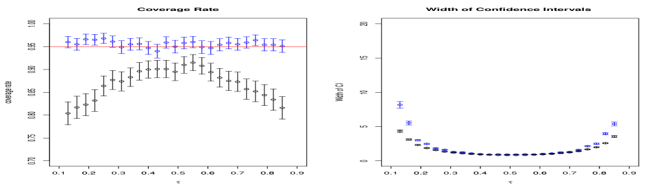
(a) Cauchy Distribution

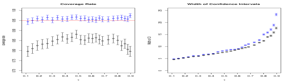
(b) Negative Binomial Distribution

Figure B1: Coverage rates and widths of 95% confidence intervals for $\theta_{0}=F^{-1}(\zeta)$ of an (unknown) distribution $F$ for a range of percentile $\zeta$ values. Bars and dots colored in blue are produced by the repro samples method and those in black are by the conventional bootstrap method. In (a) $F$ is $\text{Cauchy}(0,1)$ and in (b) $F$ is $\text{NB}(2,0.1)$. Both cases have a sample size of $n=60.$ The simulations are replicated for $1000$ times. The error bars display the mean $\pm 2$ standard errors.

 Example B2 (Robust method for contaminated Gaussian data).

Suppose the observations $\bm{y}_{obs}=(y_{1},\ldots,$ $y_{n})^{\top}$ in Example B1 are from $N(\mu_{0},\sigma_{0}^{2})$, a small percentage of which, however, are contaminated. If $I(Y_{i}\leq\mu_{0})\sim{\rm Bernoulli}(.5)$ remains hold for the contaminated $Y_{i}$’s, the approach in Example B1 can be directly applied to obtain a confidence set for $\mu_{0}$ with $\zeta=.5$. That is, a level-$\alpha$ confidence interval for $\mu_{0}$ is

$$\big{\{}\mu:a_{L}(.5)\leq\sum_{i=1}^{n}I(y_{i}\leq\mu)\leq a_{U}(.5))\big{\}}=\big{(}y_{(a_{L}(.5))},y_{(a_{U}(.5)+1)}\big{)}$$ (B1)

where $a_{L}(\cdot)$ and $a_{U}(\cdot)$ are defined defined in (6) with $r=n$; i.e.,

$$\left(a_{L}(.5),a_{U}(.5)\right)={\arg\min}_{\left\{(i,j):\sum^{j}_{k=i}{n\choose k}\left(\frac{1}{2}\right)^{n}\geq\alpha\right\}}|j-i|.$$

This interval in (B1) corresponds to conducting the sign test on median $H_{0}:\mu=\mu_{0}$ versus $H_{a}:\mu\not=\mu_{0}$. Since the sample median has a high breakdown point $BP=0.5$, the method has a high breakdown point as well.

In cases that the assumption of $I(Y_{i}\leq\mu_{0})\sim{\rm Bernoulli}(.5)$ does not hold, we typically have $I(Y_{i}\leq\mu_{0}+\delta)\sim{\rm Bernoulli}(.5)$ instead, where $\delta=\mu_{c}-\mu_{0}$ with $\mu_{c}$ being the (population) median of the contaminated data $Y_{i}$. In this case, we may adjust the confidence interval in (B1) by $\big{\{}\mu:a_{L}(.5)\leq\sum_{i=1}^{n}I(y_{i}\leq\mu+\delta)\leq a_{U}(.5))\big{\}}=\big{(}y_{(a_{L}(.5))}-\delta,y_{(a_{U}(.5)+1)}-\delta\big{)}$. Practically, $\delta$ is often unknown, however. We need to have some empirical knowledge of $\delta$ or a way to estimate $\delta$. In our numerical studies in Section 5 for the Gaussian mixture model, for each given Gaussian component we estimate the unknown $\delta$ by $\hat{\delta}=M-\tilde{M},$ where $M$ is the sample median, and $\tilde{M}$ is the weighted sample median. Although a more sophisticated weighting scheme could be developed, for simplicity we simply assigned a weight of $1.5$ for all observations overlapping with other components. Here, we say an observation overlaps with another component if it falls in the span of any other components given the (estimated) membership matrix, where the span of a component refers to the interval from the minimum to the maximum of members in the component assigned by the membership matrix. Our empirical studies suggest that this simple weighting scheme works well in the settings of Gaussian mixture models.

To obtain a robust confidence interval for $\sigma_{0}$, we utilized a robust and consistent estimator of $\sigma_{0}$: $\hat{\sigma}={\it MAD}/\Psi_{n}^{-1}(.5)$, where ${\it MAD}={\it med}\{|y_{i}-M|:i=1,\ldots,n\}$ is the median absolute deviation, $M={\it med}\{y_{i}:i=1,\ldots,n\}$ and $\Psi_{n}(t)=P(Z_{i}-M_{z}<t)$ is the cumulative distribution function of $Z_{i}-M_{z}$, $i=1,\ldots,n$. Here, $Z_{i}\overset{iid}{\sim}N(0,1)$ and $M_{z}={\it med}\{Z_{i}:i=1,\ldots,n\}.$ We have a generalized data generating model in the form of (8),

$$\sum_{i=1}^{n}I(|Y_{i}-M|\leq\Psi_{n}^{-1}(.5)\sigma)-\sum_{i=1}^{n}U_{i}^{\prime}=0,$$

where $U^{\prime}_{i}=I\{|Z_{i}-M_{z}|\leq{\small\Psi_{n}^{-1}(.5)}\}$ are dependent Bernoulli$(.5)$ variables. Since the distribution of $\sum\nolimits_{i=1}^{n}U^{\prime}_{i}$ can be simulated, we can get a Borel interval $B_{\alpha}=[a^{\prime}_{L},a^{\prime}_{U}]$, similarly as in (6); i.e., $\left[a_{L}^{\prime},a_{U}^{\prime}\right]=\arg\min_{\left\{(l,r):P(l<\sum_{i=1}^{n}U^{\prime}_{i}<r)\geq\alpha\right\}}|r-l|$. A level-$\alpha$ confidence set of $\sigma_{0}$ is then

$$\big{\{}\sigma:a^{\prime}_{L}\leq\sum_{i=1}^{n}I(|y_{i}-M|\leq{\small\Psi_{n}^{-1}(.5)}\sigma)\leq a^{\prime}_{U}\big{\}}.$$

Since $MAD$ has a high breakdown point of 50%, the above method is expected to have a high breakdown point as well.

B-II Techniques to improve computing efficiency

In this subsection, we describe two techniques that may be used to improve the computing efficiency of the generic Algorithm 1. The first technique is using the quantile regression method for the situation when the target parameter $\theta$ is continuous. The second one specifies a condition under which a data-dependent candidate set can be used.

B-II-1 Use of quantile regression to find $B_{\alpha}(\mathop{\theta\kern-4.49997pt\hbox{$\theta$}}\nolimits)$

When the target parameter(s) are discrete, we develop in Sections 3.2 and 4.2 an effective method to significantly reduce the search space of the discrete parameters. Here, we consider the case when the target parameters are continuous. We discuss how to utilize the continuity and quantile regression techniques to side-step the issues of (grid) search of the entire parameter space.

Without loss of generality, we first assume that our parameter of interest is $\mathop{\theta\kern-4.49997pt\hbox{$\theta$}}\nolimits$ in a continuous parameter space $\Theta$ and we do not have any nuisance parameters. We further assume that $T(\bm{U},\mathop{\theta\kern-4.49997pt\hbox{$\theta$}}\nolimits)$ is a mapping from ${\cal U}\times\Theta\to{\cal T}\in\mathbb{R}$, and it is continuous in $\mathop{\theta\kern-4.49997pt\hbox{$\theta$}}\nolimits$. In this case, we can use the following technique based on quantile regression to improve the computation efficiency of the repro samples method in Algorithm 1 of Section 2.2

• Let $\pi(\mathop{\theta\kern-4.49997pt\hbox{$\theta$}}\nolimits)$ be a proposal distribution that has no-zero probability over the range of $\Theta$. In addition to $|{\cal V}|$ copies of $\bm{u}^{s}\sim\bm{U}$, we simulate $|{\cal V}|$ copies of $\mathop{\theta\kern-4.49997pt\hbox{$\theta$}}\nolimits^{s}\sim\pi(\mathop{\theta\kern-4.49997pt\hbox{$\theta$}}\nolimits)$. We then fit a level-$\alpha$ quantile regression model with $t^{s}=T(\bm{u}^{s},{\mathop{\theta\kern-4.49997pt\hbox{$\theta$}}\nolimits}^{s})$ as response and ${\mathop{\theta\kern-4.49997pt\hbox{$\theta$}}\nolimits^{s}}$ as covariates. We output the conditional level-$\alpha$ quantile, say $\widehat{C}(\alpha|\theta))$, via regression of $t^{s}$ on $\mathop{\theta\kern-4.49997pt\hbox{$\theta$}}\nolimits^{s}$. The Borel set $B_{\alpha}(\mathop{\theta\kern-4.49997pt\hbox{$\theta$}}\nolimits)$ for our repro samples method is either $(-\infty,\widehat{C}(\alpha|\theta))$ or $(\widehat{C}((1-\alpha)/2|\theta),\widehat{C}(1-(1-\alpha)/2|\theta))$.

This method is similar to Algorithm 1 of dalmasso2022 in which the authors use a quantile regression to get a level-$(1-\alpha)$ rejection region for a Neyman-Pearson test problem. The difference is that the $t^{s}$ in dalmasso2022 is computed from a test statistic while our $t^{s}$ is from a nuclear mapping function. Ours is simpler since we do not need to generate any data points $\bm{y}^{s}=G(\mathop{\theta\kern-4.49997pt\hbox{$\theta$}}\nolimits^{s},\bm{u}^{s})$, especially in cases when $\bm{y}^{s}$ is expensive to generate. dalmasso2022 showed that the output conditional level-$\alpha$ quantile (say, $\widehat{C}(\alpha|\mathop{\theta\kern-4.49997pt\hbox{$\theta$}}\nolimits))$ via regression of $t^{s}$ on $\mathop{\theta\kern-4.49997pt\hbox{$\theta$}}\nolimits^{s}$ is a level-$(1-\alpha)$ critical value, if the quantile regression estimator is consistent (koenker1994quantile; takeuchi2006nonparametric), as $|{\cal V}|\to\infty$. Similarly, in our case, if the quantile regression estimator is consistent, then $B_{\alpha}(\mathop{\theta\kern-4.49997pt\hbox{$\theta$}}\nolimits)=(-\infty,\widehat{C}(\alpha|\theta))$ or $B_{\alpha}(\mathop{\theta\kern-4.49997pt\hbox{$\theta$}}\nolimits)=(\widehat{C}((1-\alpha)/2|\theta),\widehat{C}(1-(1-\alpha)/2|\theta))$ satisfies (3).

Using the quantile regression method, we only need to calculate total $|{\cal V}|$ copies of $t^{s}=T(\bm{u}^{s},{\mathop{\theta\kern-4.49997pt\hbox{$\theta$}}\nolimits^{s}})$, instead of computing $|{\cal V}|$ copies of $T(\bm{u}^{s},{\mathop{\theta\kern-4.49997pt\hbox{$\theta$}}\nolimits})$ at each grid $\mathop{\theta\kern-4.49997pt\hbox{$\theta$}}\nolimits$ value. The method often significantly improves our computational efficiency. Here, we require that $T(\bm{u},{\mathop{\theta\kern-4.49997pt\hbox{$\theta$}}\nolimits})$ be a smooth function of ${\mathop{\theta\kern-4.49997pt\hbox{$\theta$}}\nolimits}$ to ensure the consistency of quantile regression estimators. The method holds for any $\pi(\mathop{\theta\kern-4.49997pt\hbox{$\theta$}}\nolimits)$, as long as the proposal distribution $\pi(\mathop{\theta\kern-4.49997pt\hbox{$\theta$}}\nolimits)>0$ for all $\mathop{\theta\kern-4.49997pt\hbox{$\theta$}}\nolimits\in\Theta$. Practically, we often pick a proposal distribution $\pi(\mathop{\theta\kern-4.49997pt\hbox{$\theta$}}\nolimits)$ that is easy to simulate from and also that is dispersed over the range of $\Theta$ (so that there is not a region that $\mathop{\theta\kern-4.49997pt\hbox{$\theta$}}\nolimits^{s}$ has a much smaller chance to reach than other regions in $\Theta$). For example, if $\Theta$ is a bounded set, $\pi(\mathop{\theta\kern-4.49997pt\hbox{$\theta$}}\nolimits)$ can be a uniform distribution over $\Theta$. If $\Theta$ is unbounded, $\pi(\mathop{\theta\kern-4.49997pt\hbox{$\theta$}}\nolimits)$ can be a Gaussian distribution with a large variance or a heavy-tailed distribution such as Laplace.

When $\bm{t}^{s}=T(\bm{u}^{s},{\mathop{\theta\kern-4.49997pt\hbox{$\theta$}}\nolimits}^{s})$ is a vector, we instead fit a multivariate nonparametric quantile regression using the recent work by delbarrio2022nonparametric, in which the authors adopt the optimal transport concept to define multivariate center-outward quantiles and develop a quantile regression approach. Theoretically for the multivariate case, delbarrio2022nonparametric shows that the output level-$\alpha$ conditional (nested center-outward) quantile regression contour/region, say $\widehat{C}_{\pm}(\alpha|\theta)$, is a consistent reconstruction of their population version, when $|{\cal V}|\to\infty$ and under some regularity conditions. It follows that, when $|{\cal V}|\to\infty$ and by taking $B_{n}(\mathop{\theta\kern-4.49997pt\hbox{$\theta$}}\nolimits)=\widehat{C}_{\pm}(\alpha|\theta))$, we have (3).

Finally, suppose $\mathop{\theta\kern-4.49997pt\hbox{$\theta$}}\nolimits=(\eta,{\bm{\beta}}^{\top})^{\top}$, in which $\eta$ is the parameter of interest and $\bm{\beta}$ are nuisance parameters. If the true parameter value $\eta_{0}$ is inside a continuous space ${\it\Upsilon}$ and $T_{a}(\bm{u},\bm{\theta})=T_{a}(\bm{u},(\eta,{\bm{\beta}}^{\top})^{\top})$ defined in Section 3.1 is continuous in $\eta$, we can use the same quantile regression techniques to reduce the computational burden of the profile nuclear mapping function in (12). Specifically, suppose we have simulated $|{\cal V}|$ copies of $\bm{u}^{s}\sim\bm{U}$ and $|{\cal V}|$ copies of $\eta^{s}\sim\pi(\eta)$, where $\pi(\eta)$ is a proposal distribution that has non-zero probability over the range of ${\it\Upsilon}$. For any $\bm{\beta}$, we can compute $t^{s}=T_{a}(\bm{u}^{s},(\eta^{s},{\bm{\beta}}^{\top})^{\top})$ and fit a quantile regression model with $t^{s}$ being the response and $\eta^{s}$ being the covariate. The output conditional level-$\alpha^{\prime}$ quantile can give us a level-$\alpha^{\prime}$ Borel set, based on which we can get $\Gamma_{\alpha^{\prime}}(\bm{y})$. We can then define $\nu(\bm{u};\eta,\bm{\beta},\widetilde{\bm{\beta}})$ for a given $(\bm{\beta},\tilde{\bm{\beta}})$ as in (11) and use an optimization program to get rid of $\widetilde{\bm{\beta}}$ and obtain a profile nuclear mapping function $T_{p}(\bm{u},\mathop{\theta\kern-4.49997pt\hbox{$\theta$}}\nolimits)$ as defined in (12). In the situation when $\eta$ is continuous, this method can often reduce the computing effort of the direct Monte-Carlo method in Lemma 2.

B-II-2 Data dependent candidate set

Another technique for reducing the computation cost is to reduce the search space of $\Theta$, as we discussed in Section 3.2 for discrete or non-numerical parameters. In this subsection, we state a necessary condition for constructing a data-dependent candidate set (a subset of $\Theta$), say $\widehat{\Theta}(\bm{y}_{obs})$, so that we can still maintain inference validity when searching through $\widehat{\Theta}(\bm{y}_{obs})$ instead of the entire $\Theta$. Here, $\widehat{\Theta}(\bm{y}_{obs})$ is pre-screened using the observed data $\bm{y}_{obs}$. While there can be different ways to obtain this pre-screened candidate set, a key question is to overcome the potential problem of “double usage” of the observed data. In particular, after constructing this candidate set $\widehat{\Theta}=\widehat{\Theta}(\bm{y}_{obs})$, we obtain a level-$\alpha$ confidence set as

$$\Gamma_{\alpha}^{\prime}(\bm{y}_{obs})=\widehat{\Theta}(\bm{y}_{obs})\cap\Gamma_{\alpha}(\bm{y}_{obs})$$

$$\qquad=\big{\{}\mathop{\theta\kern-4.49997pt\hbox{$\theta$}}\nolimits:\exists\,\bm{u}^{*}\in{\cal U},\mathop{\theta\kern-4.49997pt\hbox{$\theta$}}\nolimits\in\widehat{\Theta},\,\hbox{s.t.}\,\bm{y}_{obs}=G_{z}({\mathop{\theta\kern-4.49997pt\hbox{$\theta$}}\nolimits},\bm{u}^{*}),\,T(\bm{u}^{*},\mathop{\theta\kern-4.49997pt\hbox{$\theta$}}\nolimits)\in B_{\alpha}(\mathop{\theta\kern-4.49997pt\hbox{$\theta$}}\nolimits)\big{\}}.$$ (B2)

Here, the “double usage” refers to the fact that we use the observed data in constructing both the candidate set $\widehat{\Theta}(\bm{y}_{obs})$ and confidence set $\Gamma_{\alpha}(\bm{y}_{obs})$.

To achieve our goal, a necessary condition that we impose on our data-dependent candidate set is

$$\mathbb{P}\big{\{}\mathop{\theta\kern-4.49997pt\hbox{$\theta$}}\nolimits_{0}\in\widehat{\Theta}(\bm{Y})\big{\}}=1-o(\delta^{\prime}),$$ (B3)

where $\delta^{\prime}>0$ is a small number as described in Theorem 1. The corollary below suggests that $\Gamma_{\alpha}^{\prime}(\bm{y}_{obs})$ in (B-II Techniques to improve computing efficiency) remains to be an (approximate) level-$\alpha$ confidence set. The result applies to both situations when $\theta$ is continuous or discrete (or non-numerical). This corollary (or a slight extension to accommodate possible nuisance parameters) has been implicitly used in the proofs of Sections 3.2, 4.2, and 4.3.

Corollary 5.

Let $\bm{Y}=G(\bm{U},\mathop{\theta\kern-4.49997pt\hbox{$\theta$}}\nolimits_{0})$ and $\widehat{\Theta}=\widehat{\Theta}(\bm{Y})$ is a candidate set that satisfies (B3). Then, we have $\mathbb{P}\big{\{}\mathop{\theta\kern-4.49997pt\hbox{$\theta$}}\nolimits_{0}\in\Gamma_{\alpha}^{\prime}(\bm{Y})\big{\}}\geq\alpha-o(\delta^{\prime}).$

Proof of Corollary 5.

By the fact that $\mathbb{P}\big{\{}T(\bm{U},\mathop{\theta\kern-4.49997pt\hbox{$\theta$}}\nolimits_{0})\in B_{\alpha}(\mathop{\theta\kern-4.49997pt\hbox{$\theta$}}\nolimits_{0})\big{\}}\geq\alpha,$ we have

$$\mathbb{P}\big{\{}T(\bm{U},\mathop{\theta\kern-4.49997pt\hbox{$\theta$}}\nolimits_{0})\in B_{\alpha}(\mathop{\theta\kern-4.49997pt\hbox{$\theta$}}\nolimits_{0})\big{\}} =\mathbb{P}\big{\{}T(\bm{U},\mathop{\theta\kern-4.49997pt\hbox{$\theta$}}\nolimits_{0})\in B_{\alpha}(\mathop{\theta\kern-4.49997pt\hbox{$\theta$}}\nolimits_{0}),\mathop{\theta\kern-4.49997pt\hbox{$\theta$}}\nolimits_{0}\in\widehat{\Theta}\big{\}}+\mathbb{P}\big{\{}T(\bm{U},\mathop{\theta\kern-4.49997pt\hbox{$\theta$}}\nolimits_{0})\in B_{\alpha}(\mathop{\theta\kern-4.49997pt\hbox{$\theta$}}\nolimits_{0}),\mathop{\theta\kern-4.49997pt\hbox{$\theta$}}\nolimits_{0}\not\in\widehat{\Theta}\big{\}}$$

$$=\mathbb{P}\big{\{}\theta_{0}\in\Gamma_{\alpha}^{\prime}(\bm{Y})\big{\}}+\mathbb{P}\big{\{}T(\bm{U},\mathop{\theta\kern-4.49997pt\hbox{$\theta$}}\nolimits_{0})\in B_{\alpha}(\mathop{\theta\kern-4.49997pt\hbox{$\theta$}}\nolimits_{0}),\mathop{\theta\kern-4.49997pt\hbox{$\theta$}}\nolimits_{0}\not\in\widehat{\Theta}\big{\}}\geq\alpha.$$

It then follows that $\mathbb{P}\big{\{}\theta_{0}\in\Gamma_{\alpha}^{\prime}(\bm{Y})\big{\}}\geq\alpha-\mathbb{P}\big{\{}T(\bm{U},\mathop{\theta\kern-4.49997pt\hbox{$\theta$}}\nolimits_{0})\in B_{\alpha}(\mathop{\theta\kern-4.49997pt\hbox{$\theta$}}\nolimits_{0}),\mathop{\theta\kern-4.49997pt\hbox{$\theta$}}\nolimits_{0}\not\in\widehat{\Theta}\big{\}}\geq\alpha-\mathbb{P}\big{\{}\theta_{0}\not\in\widehat{\Theta}\big{\}}$ and thus Corollary 5. ∎

If the size of the candidate set $\widehat{\Theta}(\bm{y}_{obs})$ is much smaller than that of $\Theta$, we can significantly lower the computing cost of Algorithm 1 and related computations, by only considering $\mathop{\theta\kern-4.49997pt\hbox{$\theta$}}\nolimits\in\widehat{\Theta}$. This reduction is particularly achievable when the parameter space is discrete. In Sections 3.2 and 4.2, we discuss an inherent “many-to-one” mapping in the repro samples method, based on which we can effectively obtain candidate sets that satisfies (B3). These candidate sets can significantly reduce the search space for discrete parameters and also accommodate cases with additional nuisance parameters.

Appendix C: A Brief Review and Comparison with Existing and Relevant Inference Procedures

The repro samples method is a (pure) frequentist approach, but its development inherits some key ideas from several existing inferential procedures across Bayesian, fiducial, and frequentist (BFF) paradigms. For readers’ convenience, we first provide in Appendix C-I a brief review of several relevant BFF inferential approaches. We then provide in Appendix C-II a comparative discussion to highlight the strengths and uniqueness of the proposed repro samples method. We also describe a role that the repro samples method can play in bridging across BFF inference approaches.

C-I A Brief Review of Existing and Relevant BFF procedures

The repro samples method is a framework that utilizes artificial sample sets for inference, and there are several relevant artificial sample-based inferential approaches across the BFF paradigms. Several relevant and important ones are briefly reviewed below.

(i) Approximate Bayesian Computing (ABC) refers to a family of techniques used to approximate posterior densities of $\mathop{\theta\kern-4.49997pt\hbox{$\theta$}}\nolimits$ by bypassing direct likelihood evaluations (cf. Rubin1984; Tavare1997; csillery2010approximate; Peters2012). A basic version of the so-called rejection ABC algorithm has the following [a] - [c] steps:

• [Step a] Simulate an artificial model parameter $\mathop{\theta\kern-4.49997pt\hbox{$\theta$}}\nolimits^{*}$ from a prior distribution $\pi(\mathop{\theta\kern-4.49997pt\hbox{$\theta$}}\nolimits)$ and, given the simulated $\mathop{\theta\kern-4.49997pt\hbox{$\theta$}}\nolimits^{*}$, simulate an artificial data set ${\bf y}^{*}$ (e.g., set ${\bf y}^{*}=G(\mathop{\theta\kern-4.49997pt\hbox{$\theta$}}\nolimits^{*},{\bf u}^{*})$ for a simulated ${\bf u}^{*}$); [Step b] If ${\bf y}^{*}\approx{\bf y}_{obs}$, we collect the artificial parameter $\mathop{\theta\kern-4.49997pt\hbox{$\theta$}}\nolimits^{*}$; [Step c] Repeat Steps [a] and [b] to obtain a large set of $\mathop{\theta\kern-4.49997pt\hbox{$\theta$}}\nolimits^{*}$.

ABC is in fact a Bayesian inversion method, since keeping $\mathop{\theta\kern-4.49997pt\hbox{$\theta$}}\nolimits^{*}$ that has the match ${\bf y}^{*}\approx{\bf y}_{obs}$ is equivalent to keep the $\mathop{\theta\kern-4.49997pt\hbox{$\theta$}}\nolimits^{*}$ that solves $G(\mathop{\theta\kern-4.49997pt\hbox{$\theta$}}\nolimits,{\bf u}^{*})\approx{\bf y}_{obs}$.

Operationally, because it is difficult to match ${\bf y}^{*}\approx{\bf y}_{obs}$, the ABC method instead suggests to match $|S({\bf y}_{obs})-S({\bf y}^{*})|\leq\epsilon$ for a pre-chosen summary statistic $S(\cdot)$ and tolerance $\epsilon>0$. The kept $\mathop{\theta\kern-4.49997pt\hbox{$\theta$}}\nolimits^{*}$ form an ABC posterior, $p_{\epsilon}(\mathop{\theta\kern-4.49997pt\hbox{$\theta$}}\nolimits|\bm{y}_{obs})$. If $S(\cdot)$ is a sufficient statistic, then the ABC posterior $p_{\epsilon}(\mathop{\theta\kern-4.49997pt\hbox{$\theta$}}\nolimits|\bm{y}_{obs})\to p(\mathop{\theta\kern-4.49997pt\hbox{$\theta$}}\nolimits|\bm{y}_{obs})$, the target posterior distribution, as $\epsilon\to 0$ at a fast rate (Barber2015; Li2016). To improve its computing efficiency, this basic ABC algorithm has been extended to, for instance, more complex ABC-Markov Chain Monte Carlo (ABC-MCMC) type of algorithms, but the key matching and Bayesian inversion ideas remain. Note that, the ABC method seeks to match each single artificial sample copy $\bm{y}^{*}$ with the observed data $\bm{y}_{obs}$ through a summary statistic and a preset tolerance level $\epsilon$ to form a rejection rule.

There are two remaining issues unsolved in the ABC method (cf., Li2016; Thornton2018). First, When $S(\cdot)$ is not sufficient, $p_{\epsilon}(\mathop{\theta\kern-4.49997pt\hbox{$\theta$}}\nolimits|\bm{y}_{obs})\not\to p(\mathop{\theta\kern-4.49997pt\hbox{$\theta$}}\nolimits|\bm{y}_{obs})$. In this case, there is no guarantee that an ABC posterior is a Bayesian posterior, thus the interpretation of the inferential result by the ABC posterior is unclear. However, it is not possible to derive a sufficient statistic when the likelihood is intractable. Thus, the requirement that $S(\cdot)$ is sufficient places a limitation on the practical use of the ABC method (as a likelihood-free inference approach). Second, the ABC method requires the preset threshold value $\epsilon\to 0$ at a fast rate, leading to a degeneracy of computing efficiency. This is because the acceptance probability in Step [b] goes to $0$ for a very small $\epsilon\to 0$, In practice, there is no clear-cut choice for an appropriate $\epsilon$ to balance the procedure’ computational efficiency and inference validity. It remains to be an unsolved question in the literature (e.g., Li2016).

(ii) Generalized fiducial inference (GFI) is a generalization of Fisher’s fiducial method, which is understood in contemporary statistics as an inversion method to solve a pivot equation for model parameter $\mathop{\theta\kern-4.49997pt\hbox{$\theta$}}\nolimits$ (Zabell1992; Hannig2016). The GFI method extends the inversion approach from a pivot to actual data; i.e., it solves for $\mathop{\theta\kern-4.49997pt\hbox{$\theta$}}\nolimits^{*}$ from ${\bf y}_{obs}=G(\mathop{\theta\kern-4.49997pt\hbox{$\theta$}}\nolimits,{\bf u}^{*})$ for artificially generated ${\bf u}^{*}$’s. However, since a solution is not always possible, the GFI method proposes to consider an optimization under an $\epsilon$-approximation:

$$\mathop{\theta\kern-4.49997pt\hbox{$\theta$}}\nolimits_{\epsilon}^{*}={\rm argmin}_{\theta\in\{\theta:\,\,||{\bf y}_{obs}-G(\theta,{\bf u}^{*})||^{2}\leq\epsilon\}}||{\bf y}_{obs}-G({\theta},{\bf u}^{*})||^{2}$$ (C1)

and let $\epsilon\to 0$ at a fast rate (Hannig2016). The GFI method many times has a guaranteed statistical (frequentist) performance, provided the sample size $n\to\infty$ and $G$ is smooth/differentiable in $\mathop{\theta\kern-4.49997pt\hbox{$\theta$}}\nolimits$ (Hannig2009; Hannig2016). Different than the ABC method that uses the rejection sampling approach, the GFI uses an optimization to approximately solve the equation $\bm{y}_{obs}=G(\mathop{\theta\kern-4.49997pt\hbox{$\theta$}}\nolimits,\bm{u}^{*})$ within a $\epsilon$-constrained set in $\Theta$. Operationally, the GFI method suffers the same computational issue as in the ABC method on the choice of the pre-specified $\epsilon$, since, as $\epsilon\to\infty$ at a fast rate, equation (C1) may not have a solution.

(iii) Efron’s bootstrap and other related artificial sampling methods, in which many copies of artificial data are generated, are a popular way to help quantify uncertainty in complicated estimation problems in statistics. Let $\hat{\bm{\theta}}({\bm{y}}_{obs})$ be a point estimator of the true parameter $\mathop{\theta\kern-4.49997pt\hbox{$\theta$}}\nolimits_{0}$ and $\mathop{\theta\kern-4.49997pt\hbox{$\theta$}}\nolimits^{*}=\hat{\mathop{\theta\kern-4.49997pt\hbox{$\theta$}}\nolimits}(\bm{y}^{*})$ be the corresponding bootstrap estimator calculated using a bootstrap sample $\bm{y}^{*}$. The key validity justification of bootstrap methods relies on the so-called bootstrap central limit theorem (CLT) (e.g., Singh1981; Bickel1981):

$$\hat{\mathop{\theta\kern-4.49997pt\hbox{$\theta$}}\nolimits}(\bm{Y}^{*})-\hat{\bm{\theta}}({\bm{y}}_{obs})|\hat{\bm{\theta}}({\bm{y}}_{obs})\sim\hat{\bm{\theta}}(\bm{Y})-\mathop{\theta\kern-4.49997pt\hbox{$\theta$}}\nolimits_{0}|\mathop{\theta\kern-4.49997pt\hbox{$\theta$}}\nolimits_{0},$$

in which the (multinomial distributed) uncertainty in resampled artificial data $\bm{Y}^{*}$ asymptotically matches the (often non-multinomial distributed) uncertainty in $\hat{\mathop{\theta\kern-4.49997pt\hbox{$\theta$}}}\nolimits(\bm{Y})$ inherited from the target random sample $\bm{Y}$. When the CLT does not apply (e.g., the parameter space $\Theta$ is a discrete set), the bootstrap methods are not supported by theory and often perform poorly.

Furthermore, the repro samples method is also related the so-called Inferential Model (IM) that seeks to produce (epistemic) probabilistic inference for $\mathop{\theta\kern-4.49997pt\hbox{$\theta$}}\nolimits_{0}$:

(iv) Inferential model (IM) is an attempt to develop a general framework for “prior-free exact probabilistic inference” (Martin2015). As described in Martin2015 and under the model assumption (1), an IM procedure include three steps:

• [A-step] Associate $(\bm{Y},\mathop{\theta\kern-4.49997pt\hbox{$\theta$}}\nolimits)$ with the unobserved auxiliary statistic $\bm{U}$, i.e., $\bm{Y}=G({\mathop{\theta\kern-4.49997pt\hbox{$\theta$}}\nolimits},{\bm{U}})$; [P-Step] Predict the unobserved auxiliary statistic $\bm{U}$ with a random set ${\cal S}$ with distribution ${\mathbb{P}}_{\cal S}$; [C-step] Combine observed $\bm{y}_{obs}$ with random set ${\cal S}$ into a new data-dependent random set $\Theta_{\bm{y}_{obs}}({\cal S})=\bigcup_{\bm{u}\in{\cal S}}\left\{\mathop{\theta\kern-4.49997pt\hbox{$\theta$}}\nolimits:\bm{y}_{obs}=G(\mathop{\theta\kern-4.49997pt\hbox{$\theta$}}\nolimits,\bm{u})\right\}$.

A novel aspect of the IM development that is different than a typical fiducial procedure is that the uncertainty quantification of $\bm{Y}$ is through the parameter-free $\bm{U}$ using a random set in [P-step]. This separation removes the impact of parameter $\bm{\theta}$ and makes the task of uncertainty quantification easier. In order to fully express the outcomes in probabilistic forms, the IM development needs to use a system of imprecise probability known as Dempster-Shafer Calculus. The outcomes of an IM algorithm are the so-called plausible and belief functions (or lower and upper probability functions) for $\mathop{\theta\kern-4.49997pt\hbox{$\theta$}}\nolimits_{0}$, which can be used for frequentist inference. The plausible and belief functions are akin to the so-called upper or lower confidence distributions (e.g., Thornton2022), although the IM method is not considered by most (including Martin and Liu) as a frequentist development.

In addition to the four reviewed methods, the repro samples also has some connections to the universal inference (wasserman2020universal) and conformal prediction (shafer2008tutorial) approaches, which be further discussed in the next subsection.

C-II Repro samples method and Connections to BFF Inferential Approaches

The repro samples method borrows two important ideas from the aforementioned BFF procedures. First, the repro samples method utilizes artificial data samples to help quantify the uncertainty of statistical inference. This idea has been used in the bootstrap, ABC, GFI, and Monte-Carlo hypothesis testing procedures, among others. A key aspect of utilizing artificial data samples for inference in these procedures is the common attempt to match (in a certain way) the artificial data with the observed sample. See Thornton2022 for a more elaborated discussion. This matching is done by directly comparing either the value or distribution of the artificial $\bm{y}^{*}$ (or its summary statistic) with that of $\bm{y}_{obs}$ (or its summary statistic). The proposed repro samples method fully utilizes the artificial samples and the matching idea to both develop inference and solve computational questions. In addition, the repro samples method also borrows an idea from the IM development to quantify the inference uncertainty by first assessing the uncertainty of the unobserved $\bm{u}^{rel}$. These two important ideas have guided us to develop both finite and asymptotic inferences under the frequentist framework without the need to use any likelihood or decision theoretical criteria. We consider that the repro samples method is a further development (generalization and refinements) of these aforementioned existing BFF procedures.

In the remaining of this subsection, we provide some comparative discussions, comparing the repro samples method with: (i) the ABC and GFI methods; (ii) the IM method; (iii) the universal inference method; (iv) the conformal prediction approach; and (v) the Monte-Carlo hypothesis testing procedure. We further describe the role that the repro samples method can play in bridging across BFF inference approaches.

(i) Repro samples method versus ABC and GFI methods. Both the GFI and repro samples approach highlight the matching of equation $\bm{y}_{obs}=G(\mathop{\theta\kern-4.49997pt\hbox{$\theta$}}\nolimits,\bm{u}^{*})$ and the fact that when $\bm{u}^{*}$ matches or is close to $\bm{u}^{rel}$, the solution of $\mathop{\theta\kern-4.49997pt\hbox{$\theta$}}\nolimits$ from the equation is equal or close to the true $\mathop{\theta\kern-4.49997pt\hbox{$\theta$}}\nolimits_{0}$. The difference lies in that the GFI approach compares each single copy of artificial sample $\bm{y}^{*}=G(\mathop{\theta\kern-4.49997pt\hbox{$\theta$}}\nolimits,\bm{u}^{*})$ with the single copy of the observed $\bm{y}_{obs}$, so does the ABC method. In the Monte-Carlo implementation of the repro samples method (e.g., Algorithm 1), however, we compare the single copy of the observed $\bm{y}_{obs}$ with multiple copies of $\bm{y}^{s}=G(\mathop{\theta\kern-4.49997pt\hbox{$\theta$}}\nolimits,\bm{u}^{s})$ (or, more accurately, the realized $T(\mathop{\theta\kern-4.49997pt\hbox{$\theta$}}\nolimits,\bm{u}^{rel})$ with multiple copies of $T(\mathop{\theta\kern-4.49997pt\hbox{$\theta$}}\nolimits,\bm{u}^{s})$’s), for $\bm{u}^{s}\in{\cal V}$, where ${\cal V}$ is the collection of many copies of $\bm{u}^{s}$. By comparing observed sample $\bm{y}_{obs}$ (or realized $\bm{u}^{rel}$) with many copies of artificially generated $\bm{y}^{s}=G(\mathop{\theta\kern-4.49997pt\hbox{$\theta$}}\nolimits,\bm{u}^{s})$ (or $\bm{u}^{s}\in{\cal V}$), it allows us to use a confidence level $\alpha$ to calibrate the uncertainty thus side-step the difficult issue in both GFI and ABC methods on how to appropriately preset the threshold $\epsilon$. Furthermore, the use of the nuclear mapping adds much flexibility to the repro samples method. Unlike the ABC method, the often inconvenient requirement of using a sufficient statistic to ensure inference validity is not needed for the repro samples method. Additionally, the repro samples method is a frequentist method. It does not need to make the additional model assumption of a prior distribution. It also avoids the potential philosophical issues that are often associated with fiducial inference on its interpretations.

(ii) Repro samples method versus IM method. The repro samples and IM methods both promote first quantifying the uncertainty of $\bm{U}$ and use it to help address the overall uncertainty inherited in the sampling data. To produce a level $\alpha$ confidence set, the repro sample method uses a single fixed Borel set and a $\mathop{\theta\kern-4.49997pt\hbox{$\theta$}}\nolimits$-dependent nuclear mapping function to help quantify the uncertainty in $\bm{U}$. Moreover, the repro samples method is a fully frequentist approach developed using only the standard probability tool. The IM method, on the other hand, attempts to achieve a higher level goal of producing a prior-free probabilistic inference for the unknown parameter $\mathop{\theta\kern-4.49997pt\hbox{$\theta$}}\nolimits$. To achieve this goal, it requires to use random sets and a complex imprecise probability system known as Dempster-Shafer calculus. Furthermore, the IM method focuses on finite sample inference, while the repro samples can be used for both finite and large sample inferences. In addition, the introduction and promotion of the so-called nuclear mapping function in the repro samples method allows it to greatly extend the scope of the inferential framework, making it more flexible and effective for many complex inference problems in both statistics and data science. Finally, the repro samples method emphasizes the actual matching of simulated artificial $\bm{u}^{*}$ with the (unknown) realized $\bm{u}^{rel}$ as well. The development of candidate set for discrete parameter $\eta$ in Section 3.2 is rooted in the fact that when $\bm{u}^{*}$ is equal or in a neighborhood of $\bm{u}^{rel}$ can give us the same $\eta_{0}$ in the many-to-one mapping function (15). This matching scheme cannot be easily adapted in an IM approach.

(iii) Repro samples method versus universal inference approach. Universal inference (wasserman2020universal) is a framework recently developed to provide performance-guaranteed inferences without regularity conditions. The universal inference method typically requires a tractable likelihood function and data splitting. It relies on a Markov inequality to justify its validity (testing size), at some expanse of power (Dunn2022; TseDavison2023). The framework can handle irregular inference problems and is particularly effective for sequential testing problems (ramdas2020admissible; Xie2023Discussion). The case study example of Gaussian mixture is also studied in wasserman2020universal but, unlike the repro samples method, it cannot provide a two-sided confidence set for the unknown number of components $\tau_{0}$. The repro samples method is a likelihood-free approach that is also effective for irregular inference problems, and it does not systemically suffer a loss of power while maintaining inference validity.

(iv) Repro samples method versus conformal prediction method. Conformal prediction is a popular nonparametric prediction method used to construct a level-$\alpha$ confidence set for a future (unobserved) observation, say $y_{new}$, given observed $n$ exchangeable data points $\{y_{1},\ldots,y_{n}\}$ (vovk2005algorithmic; shafer2008tutorial). Particularly, for a potential value $y$ of $y_{new}$, if it is within a $\alpha$-level central region of $\{y_{1},\ldots,y_{n}\}$, then the value $y$ is conformal with $\{y_{1},\ldots,y_{n}\}$ at the $\alpha$-level. The collection of such $y$ values forms a level-$\alpha$ predictive set of $y_{new}$. In our case, we are interested in a fixed unknown parameter $\mathop{\theta\kern-4.49997pt\hbox{$\theta$}}\nolimits_{0}$, instead of a random $y_{new}$. Nevertheless, we can use the same conformal concept to intuitively explain the Monte-Carlo repro samples approach (cf., Algorithm 1 in Section 2.2): For a potential value $\mathop{\theta\kern-4.49997pt\hbox{$\theta$}}\nolimits$ of $\mathop{\theta\kern-4.49997pt\hbox{$\theta$}}\nolimits_{0}$, we generate $|{\cal V}|$ sets of artificial data $\bm{y}^{s}=G(\mathop{\theta\kern-4.49997pt\hbox{$\theta$}}\nolimits,\bm{u}^{s})$ (or, more accurately, $|{\cal V}|$ copies of $T(\mathop{\theta\kern-4.49997pt\hbox{$\theta$}}\nolimits,\bm{u}^{s})$’s), for $\bm{u}^{s}\in{\cal V}$; If the observed data set $\bm{y}_{obs}$ is conformal with the $|{\cal V}|$ artificial data sets $\bm{y}_{s}$’s (or, more accurately, if there exists an $\bm{u}^{*}\in{\cal U}$ such that $\bm{y}_{obs}=G(\mathop{\theta\kern-4.49997pt\hbox{$\theta$}}\nolimits,\bm{u}^{*})$ and the value $T(\bm{u}^{*},\mathop{\theta\kern-4.49997pt\hbox{$\theta$}}\nolimits)$ is conformal with multiple copies of $T(\mathop{\theta\kern-4.49997pt\hbox{$\theta$}}\nolimits,\bm{u}^{s})$’s), for $\bm{u}^{s}\in{\cal V}$, we collect the $\mathop{\theta\kern-4.49997pt\hbox{$\theta$}}\nolimits$ value. The collection of such $\mathop{\theta\kern-4.49997pt\hbox{$\theta$}}\nolimits$ values forms a level-$\alpha$ confidence set of $\mathop{\theta\kern-4.49997pt\hbox{$\theta$}}\nolimits_{0}$.

(v) Repro samples method versus the classical Monte-Carlo hypothesis testing approach. As stated in (iv) above, the Monte-Carlo Algorithm 1 for the repro samples method in Section 2.2 can be described as follows: for any potential value $\mathop{\theta\kern-4.49997pt\hbox{$\theta$}}\nolimits\in\Theta$, we generate multiple copies of $\bm{u}^{s}$ (denote the set of their collection ${\cal V}$) and compute corresponding $T(\bm{u}^{s},\mathop{\theta\kern-4.49997pt\hbox{$\theta$}}\nolimits)$’s. If there exists an $\bm{u}^{*}\in{\cal U}$ such that $\bm{y}_{obs}=G(\mathop{\theta\kern-4.49997pt\hbox{$\theta$}}\nolimits,\bm{u}^{*})$ and the value $T(\bm{u}^{*},\mathop{\theta\kern-4.49997pt\hbox{$\theta$}}\nolimits)$ is conformal with the multiple copies of $T(\bm{u}^{s},\mathop{\theta\kern-4.49997pt\hbox{$\theta$}}\nolimits)$, $\bm{u}^{s}\in{\cal V}$, at the level $\alpha$, then we keep the $\mathop{\theta\kern-4.49997pt\hbox{$\theta$}}\nolimits$ in $\Gamma_{\alpha}(\bm{y}_{obs})$. Here, the matching of a single copy of $T(\bm{u}^{*},\mathop{\theta\kern-4.49997pt\hbox{$\theta$}}\nolimits)$ with the multiple copies of $T(\bm{u}^{s},\mathop{\theta\kern-4.49997pt\hbox{$\theta$}}\nolimits)$’s is evaluated by a conformal measure at level-$\alpha$. Here, the concept of “conformal” is the same as in the recent development of conformal prediction (vovk2005algorithmic).

In the special case when the nuclear mapping is defined through a test statistic $T(\bm{u},\mathop{\theta\kern-4.49997pt\hbox{$\theta$}}\nolimits)=\tilde{T}(\bm{y},\mathop{\theta\kern-4.49997pt\hbox{$\theta$}}\nolimits)$ where $\bm{y}=G(\mathop{\theta\kern-4.49997pt\hbox{$\theta$}}\nolimits,\bm{u})$ (as discussed in Section 6) and also that we can always find a $\bm{u}^{*}\in{\cal U}$ such that $\bm{y}_{obs}=G(\mathop{\theta\kern-4.49997pt\hbox{$\theta$}}\nolimits,\bm{u}^{*})$ for any $\mathop{\theta\kern-4.49997pt\hbox{$\theta$}}\nolimits$, the Monte-Carlo Algorithm 1 is simplified to: for any potential value $\mathop{\theta\kern-4.49997pt\hbox{$\theta$}}\nolimits\in\Theta$, we generate $|{\cal V}|$ copies of artificial data $\bm{y}^{s}=G(\mathop{\theta\kern-4.49997pt\hbox{$\theta$}}\nolimits,\bm{u}^{s})$ and compute the corresponding $\tilde{T}(\bm{y}^{s},\mathop{\theta\kern-4.49997pt\hbox{$\theta$}}\nolimits)$, for $\bm{u}^{s}\in{\cal V}$. If the test statistic $\tilde{T}(\bm{y}_{obs},\mathop{\theta\kern-4.49997pt\hbox{$\theta$}}\nolimits)$ is conformal with the many copies of $\tilde{T}(\bm{y}^{s},\mathop{\theta\kern-4.49997pt\hbox{$\theta$}}\nolimits)$’s at level $\alpha$, then we keep this $\mathop{\theta\kern-4.49997pt\hbox{$\theta$}}\nolimits$ to form the level-$\alpha$ confidence set $\Gamma_{\alpha}(\bm{y}_{obs})$. It is easy to see that this simplified algorithm is equivalent to a Monte-Carlo implementation of the classical hypothesis test of $H_{0}:\mathop{\theta\kern-4.49997pt\hbox{$\theta$}}\nolimits_{0}=\mathop{\theta\kern-4.49997pt\hbox{$\theta$}}\nolimits$, where the conformal statement above corresponds to the statement of not rejecting $H_{0}$. Again, we see that the classical testing approach is a special case of our repro samples method. In the Monte-Carlo version, we utilize multiple copies of artificial samples $\bm{y}^{s}$’s and compare them to a single copy of the observed data $\bm{y}_{obs}$.

Finally, as an artificial-sample-based inference procedure, the repro samples method plays a role in bridging across BFF inference approaches.

Artificial-sample-based inference and a bridge of BFF paradigms. There have been several recent developments on the foundation of statistical inference across Bayesian, fiducial, and frequentist (BFF) paradigms. Reid2022 and Thornton2022 provide comprehensive overviews on several recent BFF research developments at the foundation level. Based on the development of confidence distribution, Thornton2022 also explores the aspect of making inferences through matching artificial samples with observed data across BFF procedures. It argues that the matching of simulated artificial randomness with the sampling randomness inherited from a statistical model provides a unified bridge to connect BFF inference procedures. Here, the artificial randomness includes, for example, bootstrap randomness in bootstrap, MCMMC randomness in a Bayesian analysis, the randomness of $\bm{U}^{*}$ in fiducial procedures such as the GFI and IM methods. The repro samples method is another development that seeks to align simulated artificial randomness with the sampling randomness. By doing so we can effectively measure and quantify the uncertainty in our statistical inferential statements. The repro samples method can be used to address many difficult inference problems, especially those involving discrete parameter space and also those where large sample CLT does not apply. It provides a further advancement on the foundation of statistical inference to meet the growing need for ever-emerging data science.

References

- (1)
- Barber et al. (2015) Barber, S., Voss, J. and Webster, M. (2015), ‘The rate of convergence for approximate bayesian computation’, Electronic Journal of Statistics 9(1), 80–105.
- Bickel and Freedman (1981) Bickel, P. J. and Freedman, D. (1981), ‘Some asymptotic theory for the bootstrap’, Annals of Statistics 9, 1196–1217.
- Casella and Berger (1990) Casella, G. and Berger, R. L. (1990), Statistical Inference, Wadsworth and Brooks/Cole, Pacific Grove, CA.
- Chandra et al. (2024) Chandra, O., DasGupta, T. and Xie, M. (2024), ‘Finite sample exact confidence sets for population ranks’, Working paper .
- Chen et al. (2012) Chen, J., Li, P. and Fu, Y. (2012), ‘Inference on the Order of a Normal Mixture’, Journal of the American Statistical Association 107(499), 1096–1105.
- Chuang and Lai (2000) Chuang, C.-S. and Lai, T. L. (2000), ‘Hybrid resampling methods for confidence intervals’, Statistica Sinica 10, 1–50.
- Cox and Reid (1987) Cox, D. R. and Reid, N. (1987), ‘Parameter orthogonality and approximate conditional inference’, Journal of the Royal Statistical Society. Series B (Methodological) 49(1), 1–39.
- Csilléry et al. (2010) Csilléry, K., Blum, M. G., Gaggiotti, O. E. and François, O. (2010), ‘Approximate bayesian computation (abc) in practice’, Trends in ecology & evolution 25(7), 410–418.
- Dalmasso et al. (2022) Dalmasso, N., Masserano, L., Zhao, D., Izbicki, R. and Lee, A. B. (2022), ‘Likelihood-Free Frequentist Inference: Confidence Sets with Correct Conditional Coverage’. arXiv:2107.03920 [cs, stat].
- Davison (2003) Davison, A. (2003), Statistical Models, Cambridge University Press.
- del Barrio et al. (2022) del Barrio, E., Sanz, A. G. and Hallin, M. (2022), ‘Nonparametric multiple-output center-outward quantile regression’.
- Dudley et al. (1991) Dudley, C. R., Giuffra, L. A., Raine, A. E. and Reeders, S. T. (1991), ‘Assessing the role of APNH, a gene encoding for a human amiloride-sensitive Na+/H+ antiporter, on the interindividual variation in red cell Na+/Li+ countertransport.’, Journal of the American Society of Nephrology 2(4), 937–943.
- Dunn et al. (2022) Dunn, R., Ramdas, A., Balakrishnan, S. and Wasserman, L. (2022), ‘Gaussian universal likelihood ratio testing’, Biometrika 110(2), 319–337.
- Efron and Tibshirani (1993) Efron, B. and Tibshirani, R. J. (1993), An Introduction to the Bootstrap, Monographs on Statistics and Applied Probability, Chapman & Hall/CRC, Florida, USA.
- Fishman (1996) Fishman, G. (1996), Monte Carlo: concepts, algorithms, and applications, Springer Science & Business Media, New York, USA.
- Grün and Leisch (2007) Grün, B. and Leisch, F. (2007), ‘Fitting finite mixtures of generalized linear regressions in r’, Computational Statistics & Data Analysis 51(11), 5247–5252.
- Hallin et al. (2021) Hallin, M., del Barrio, E., Cuesta-Albertos, J. and Matrán, C. (2021), ‘Distribution and quantile functions, ranks and signs in dimension d: A measure transportation approach’, The Annals of Statistics 49(2), 1139 – 1165.
- Hannig (2009) Hannig, J. (2009), ‘On generalized fiducial inference.’, Statistica Sinica 19, 491–544.
- Hannig et al. (2016) Hannig, J., Iyer, H., Lai, R. C. S. and Lee, T. C. M. (2016), ‘Generalized fiducial inference: A review and new results’, Journal of the American Statistical Association 111(515), 1346–1361.
- Hastie and Green (2012) Hastie, D. I. and Green, P. J. (2012), ‘Model choice using reversible jump Markov chain Monte Carlo’, Statistica Neerlandica 66(3), 309–338.
- Javanmard and Montanari (2014) Javanmard, A. and Montanari, A. (2014), ‘Confidence intervals and hypothesis testing for high-dimensional regression’, The Journal of Machine Learning Research 15(1), 2869–2909.
- Kass and Raftery (1995) Kass, R. E. and Raftery, A. E. (1995), ‘Bayes factors’, Journal of the American Statistical Association 90(430), 773–795.
- Koenker et al. (1994) Koenker, R., Ng, P. and Portnoy, S. (1994), ‘Quantile smoothing splines’, Biometrika 81(4), 673–680.
- Komárek and Komárková (2014) Komárek, A. and Komárková, L. (2014), ‘Capabilities of R package mixAK for clustering based on multivariate continuous and discrete longitudinal data’, Journal of Statistical Software 59, 1–38.
- Li and Fearnhead (2018) Li, W. and Fearnhead, P. (2018), ‘On the asymptotic efficiency of approximate bayesian computation estimators’, Biometrika 105(2), 286–299.
- Liu et al. (2022) Liu, D., Liu, R. Y. and Xie, M. (2022), ‘Nonparametric fusion learning for multiparameters: Synthesize inferences from diverse sources using data depth and confidence distribution’, Journal of the American Statistical Association 117(540), 2086–2104.
- Liu et al. (1999) Liu, R. Y., Parelius, J. M. and Singh, K. (1999), ‘Multivariate analysis by data depth: Descriptive statistics, graphics and inference, (with discussion and a rejoinder by Liu and Singh)’, The Annals of Statistics 27(3), 783–858.
- Liu and Shao (2003) Liu, X. and Shao, Y. (2003), ‘Asymptotics for likelihood ratio tests under loss of identifiability’, The Annals of Statistics 31(3), 807 – 832.
- Martin and Liu (2015) Martin, R. and Liu, C. (2015), Inferential Models: Reasoning with Uncertainty, Chapman & Hall/CRC.
- Peters et al. (2012) Peters, G., Fan, Y. and Sisson, S. (2012), ‘On sequential monte carlo partial rejection control approximate bayesian computation’, Statistical Computing 22, 1209–1222.
- Pokotylo et al. (2019) Pokotylo, O., Mozharovskyi, P. and Dyckerhoff, R. (2019), ‘Depth and Depth-Based Classification with R Package ddalpha’, Journal of Statistical Software 91, 1–46.
- Powell (1986) Powell, J. L. (1986), ‘Censored regression quantiles’, Journal of Econometrics 32(1), 143–155.
- Ramdas et al. (2020) Ramdas, A., Ruf, J., Larsson, M. and Koolen, W. (2020), ‘Admissible anytime-valid sequential inference must rely on nonnegative martingales’, arXiv preprint arXiv:2009.03167 .
- Reid (2024) Reid, N. (2024), ‘distributions for parameters’, in J. Berger, X.-L. Meng, N. Reid and M. Xie, eds, ‘Handbook on Bayesian, Fiducial and Frequentist (BFF) Inferences’, Chapman & Hall.
- Reid and Cox (2015) Reid, N. and Cox, D. R. (2015), ‘On some principles of statistical inference’, International Statistical Review 83(2), 293–308.
- Richardson and Green (1997) Richardson, S. and Green, P. J. (1997), ‘On Bayesian Analysis of Mixtures with an Unknown Number of Components (with discussion)’, Journal of the Royal Statistical Society: Series B (Statistical Methodology) 59(4), 731–792.
- Robert (2016) Robert, C. P. (2016), Approximate Bayesian computation: A survey on recent results, in N. D. Cools R., ed., ‘Monte Carlo and Quasi-Monte Carlo Methods’, Vol. 163, Springer Proceedings in Mathematics Statistics, Switzerland, pp. 185–205.
- Roeder (1994) Roeder, K. (1994), ‘A Graphical Technique for Determining the Number of Components in a Mixture of Normals’, Journal of the American Statistical Association 89(426), 487–495.
- Rubin (1984) Rubin, D. B. (1984), ‘Bayesianly justifiable and relevant frequency calculations for the applied statistician’, The Annals of Statistics 12, 1151–1172.
- Shafer and Vovk (2008) Shafer, G. and Vovk, V. (2008), ‘A tutorial on conformal prediction’, Journal of Machine Learning Research 9(Mar), 371–421.
- Singh (1981) Singh, K. (1981), ‘On the asymptotic accuracy of Efron’s bootstrap’, The Annals of Statistics 9(6), 1187–1195.
- Smith (2007) Smith, J. Q. (2007), Calibration of Computer Models, John Wiley & Sons, Hoboken, NJ.
- Takeuchi et al. (2006) Takeuchi, I., Le, Q., Sears, T., Smola, A. et al. (2006), ‘Nonparametric quantile estimation’.
- Tavaré et al. (1997) Tavaré, S., Balding, D. J., Griffiths, R. C. and Donnelly, P. (1997), ‘Inferring coalescence times from dna sequence data’, Genetics 145, 505–518.
- Thornton et al. (2023) Thornton, S., Li, W. and Xie, M. (2023), ‘Approximate confidence distribution computing’, The New England Journal of Statistics in Data Science 1(2), 270–282.
- Thornton and Xie (2024) Thornton, S. and Xie, M. (2024), Bridging bayesian, frequentist and fiducial (bff) inferences using confidence distribution, in J. Berger, X.-L. Meng, N. Reid and M. Xie, eds, ‘Handbook on Bayesian, Fiducial and Frequentist (BFF) Inferences’, Chapman & Hall.
- Tse and Davison (2022) Tse, T. and Davison, A. C. (2022), ‘A note on universal inference’, Stat 11(1), e501.
- Vovk et al. (2005) Vovk, V., Gammerman, A. and Shafer, G. (2005), Algorithmic learning in a random world, Springer Science & Business Media.
- Wang et al. (2022) Wang, P., Xie, M. and Zhang, L. (2022), ‘Finite-and large-sample inference for model and coefficients in high-dimensional linear regression with repro samples’, arXiv preprint arXiv:2209.09299 .
- Wang and Blei (2019) Wang, Y. and Blei, D. (2019), ‘Variational bayes under model misspecification’, Advances in Neural Information Processing Systems 32.
- Wasserman et al. (2020) Wasserman, L., Ramdas, A. and Balakrishnan, S. (2020), ‘Universal inference’, Proceedings of the National Academy of Sciences 117(29), 16880–16890.
- Xie (2023) Xie, M. (2023), ‘Discussion on “a note on universal inference” by Drs. Timmy Tse and Anthony Davison’, Stat 12(1), e4571.
- Xie et al. (2009) Xie, M., Singh, K. and Zhang, C. (2009), ‘Confidence intervals for population ranks in the presence of ties and near ties’, Journal of the American Statistical Association 104, 775–788.
- Xie and Wang (2022) Xie, M. and Wang, P. (2022), ‘Repro Samples Method for Finite- and Large-Sample Inferences’, arXiv e-prints p. arXiv.2206.06421.
- Zabell (1992) Zabell, S. L. (1992), ‘R. a. fisher and the fiducial argument’, Statistical Science 7, 369–387.
- Zhang and Zhang (2014) Zhang, C.-H. and Zhang, S. S. (2014), ‘Confidence intervals for low dimensional parameters in high dimensional linear models’, Journal of the Royal Statistical Society: Series B (Statistical Methodology) 76(1), 217–242.