Nonsmooth Nonparametric Regression via
Fractional Laplacian Eigenmaps

Abstract

We develop nonparametric regression methods for the case when the true regression function is not necessarily smooth. More specifically, our approach is using the fractional Laplacian and is designed to handle the case when the true regression function lies in an $L_{2}$-fractional Sobolev space with order $s\in(0,1)$. This function class is a Hilbert space lying between the space of square-integrable functions and the first-order Sobolev space consisting of differentiable functions. It contains fractional power functions, piecewise constant or polynomial functions and bump function as canonical examples. For the proposed approach, we prove upper bounds on the in-sample mean-squared estimation error of order $n^{-\frac{2s}{2s+d}}$, where $d$ is the dimension, $s$ is the aforementioned order parameter and $n$ is the number of observations. We also provide preliminary empirical results validating the practical performance of the developed estimators.

1 Introduction

Laplacian based nonparametric regression is a widely used approach in machine learning that leverages the Laplacian Eigenmaps algorithm to perform regression tasks without relying on explicit parametric models. The nonparametric nature of the approach makes it flexible and adaptable to data generating process without imposing strict assumptions about the functional form of the relationship between the response and the covariates. Existing theoretical studies of this approach are restricted to establishing minimax rates of convergence and adaptivity properties when the true regression function lies in Sobolev spaces; see Section 1.1 for details. Such spaces are inherently smooth in nature and exclude important function classes in nonparametric statistics, such as piecewise constant or polynomial functions, bump functions and other such nonsmooth function classes.

In this work, using the framework of fractional Laplacians, we propose a novel approach called Principal Component Regression using Fractional Laplacian Eigenmaps (PCR-FLE) for nonsmooth and nonparametric regression. The PCR-FLE algorithm generalizes the PCR-LE algorithm by Green et al. (2023) and the PCR-WLE algorithm by Shi et al. (2024), and is designed to naturally handle the case when the true regression function lies in an $L_{2}$-fractional Sobolev space $H^{s}(\mathcal{X})$ (see Definition 2.1). Specifically, consider the following regression model, $Y_{i}=f(X_{i})+\varepsilon_{i}$, for $i=1,\ldots,n,$ where $f:\mathcal{X}\to\mathbb{R}$, $f\in H^{s}(\mathcal{X})$ for $s\in(0,1)$, $X_{i}\overset{\text{i.i.d.}}{\sim}g$, where $g$ is a density on $\mathcal{X}\subset\mathbb{R}^{d}$, and $\varepsilon_{i}\overset{\text{i.i.d.}}{\sim}N(0,1)$ is the noise (independent of the $X_{i}$’s). The goal is to estimate the regression function $f$ given pairs of observations $(X_{1},Y_{1}),\ldots,(X_{n},Y_{n})$. The proposed PCR-FLE algorithm proceeds by estimating the eigenvalues and the eigenfunction of the fractional Laplacian operator (see (6)) based on the eigenvalues and the eigenvectors of the $\epsilon$-graph constructed from the samples $\{X_{i}\}_{i=1}^{n}$, and projecting the response vector onto the top-$K$ eigenvectors.

For this procedure, we make the following technical contributions in this work:

• In Theorem 3.1, we establish upper bounds on the estimation error of the PCR-FLE algorithm in a nonparametric regression setting, when the true regression function lies in fractional Sobolev spaces of order $s\in(0,1)$. Such spaces include piecewise constant, polynomial function, bump functions and other nonsmooth function classes that are of practical importance.

• As a part of the proof of our main results in Theorem 3.1, we derive a concentration inequality of the discrete fractional Sobolev seminorm/energy to its continuum, which serves as an important quantity for many fractional Laplacian based machine learning algorithms.

We provide preliminary simulations of the proposed approach validating the performance of PCR-FLE algorithm in estimating various nonsmooth functions in Section 4. Our contributions underscore the importance of employing fractional graph Laplacians in nonsmooth nonparametric regression and lay a strong statistical groundwork for this technique. The theoretical results characterize the dependability and efficacy of this approach.

1.1 Literature review

Graph Laplacians find extensive use in various data science applications, including feature learning and spectral clustering (Weiss, 1999; Shi and Malik, 2000; Ng et al., 2001; von Luxburg, 2007). They are employed for tasks such as extracting heat kernel signatures for shape analysis (Sun et al., 2009; Andreux et al., 2015; Dunson et al., 2021), reinforcement learning (Mahadevan and Maggioni, 2007; Wu et al., 2019), and dimensionality reduction (Belkin and Niyogi, 2003; Coifman and Lafon, 2006), among others. Additional discussions can be found in works by Belkin et al. (2006); Wang et al. (2015); Chun et al. (2016); Hacquard et al. (2022).

Several papers in the recent past have focused on obtaining theoretical rates of convergence in the context of Laplacian operator estimation and related eigenvalue and/or eigenfunction estimation. Pointwise consistency under $\epsilon$-graphs have been studied by Belkin and Niyogi (2005); Hein et al. (2005); Giné and Koltchinskii (2006); Hein et al. (2007); see references therein for more related works. Furthermore, Trillos and Slepčev (2018) derives consistency properties of spectral clustering methods through studying the above spectral convergence with no specific error estimates. Following them, Shi (2015); Trillos et al. (2020); Calder and Trillos (2022) derived rates of convergences of Laplacian eigenvalues and eigenvectors to population counterparts with explicit error estimates under both $\epsilon$-graphs and $k$-NN graph. Recently, Hoffmann et al. (2022) developed a framework for extending the above convergence results to a general Laplacian family, the weighted Laplacians and Shi et al. (2024) provided additional theoretical results on the convergence of the weighted Laplacians. Green et al. (2021) considered Laplacian smoothing estimation and showed its minimax optimal rates in low-dimensional space. Green et al. (2023) proposed the principal components regression with the Laplacian eigenmaps (PCR-LE) algorithm that achieves minimax optimal rates of nonparametric regression under uniform design. The PCR-LE algorithm was later generalized by Shi et al. (2024) to the weighted Laplacians that include other commonly applied Laplacians such as the normalized Laplacian and the random walk Laplacian. Moreover, from a methodological perspective, Rice (1984) investigated spectral series regression on Sobolev spaces, and Trillos et al. (2022) applied the graph Poly-Laplacian smoothing to the regression problem.

The literature on both theoretical analysis and statistical applications fractional (graph) Laplacians is still in its infancy. Antil et al. (2021) extended the standard diffusion maps algorithm to the fractional setting that involve the use of a non-local kernel. Fractional Laplacian regularization was applied in Antil et al. (2020) to study tomographic reconstruction. Dunlop et al. (2020) studied large graph limits of semi-supervised learning problems via powers of graph Laplacian, including fractional Laplacians and provided their consistency guarantee in terms of $\Gamma$-convergence. Based on it, semi-supervised Learning with finite labels was explored in Weihs and Thorpe (2023) via minimizing the fractional Sobolev seminorm/energy and consistency of such approach was provided through showing the $\Gamma$-convergence.

There is an extensive literature on nonparametric statistics on estimating piecewise constant or polynomial functions; see, for example, Chaudhuri et al. (1994); Donoho (1997); Scott and Nowak (2006); Tibshirani (2014) and references therein for a sampling of such work. While most of this work focuses on the one or two dimensional setting, Chatterjee and Goswami (2021) recently considered the multivariate setting and established adaptive rates. Many of these contributions either consider fixed (lattice-based) designs or axis-aligned partitions. Under appropriate boundary conditions on the shape of the partition cells (not necessarily axis-aligned), piecewise constant or polynomial functions belong to fractional Sobolev spaces. Furthermore, rates of estimation in the case of Hölder and Lipschitz functions are well-studied (Györfi et al., 2002; Tsybakov, 2008). In particular, Hölder functions on bounded domains (which is typically needed in statistical estimation contexts) belong to fractional Sobolev spaces. The inclusion in the other direction is more complicated, and we refer to Rybalko (2023) for the state-of-the art results in one-dimension. Estimating functions with bounded variation, in both one and multidimensional settings is also considered in the literature; see, for example, Mammen and Van De Geer (1997); Koenker and Mizera (2004); Sadhanala et al. (2016); Hütter and Rigollet (2016); Sadhanala et al. (2017) and references therein for some representative works. In particular, a recent work by Hu et al. (2022) considered the random design setting in the multivariate case and established minimax rates. More technical details regarding the relationship between function spaces of bounded variation and fractional Sobolev spaces are provided in Section 2.4.

2 Preliminaries and Methodology

2.1 Laplacian matrices based on $\epsilon$-neighborhood graphs

For i.i.d data $X_{1},\ldots,X_{n}$ from a distribution $G$ suported on $\mathcal{X}\subseteq\mathbb{R}^{d}$ with the density $g$, the $\epsilon$-neighborhood graph is defined by setting the vertex set as $\{X_{1},\ldots,X_{n}\}$ and putting an edge on $X_{i}\sim X_{j}$ provided that $\|X_{i}-X_{j}\|\leq\epsilon$ with the weights that depend inversely on the distance between the vertices connected by them:

$$w_{i,j}^{\epsilon}:=\eta\left(\frac{\|X_{i}-X_{j}\|}{\epsilon}\right),\quad i,j=1,\ldots,n,$$ (1)

where $\|\cdot\|$ denotes the standard Euclidean norm. Here $\eta\geq 0$ is a non-increasing kernel function and $\epsilon$ is the bandwidth parameter.

The adjacency matrix is then defined as $W=(w_{i,j}^{\epsilon})_{i,j=1,\ldots,n}$ and the degree matrix $D=(d_{ij})_{i,j=1,\ldots,n}$ is then given by a diagonal matrix with the $i$-th diagonal element as $d_{i}:=\sum_{j=1}^{n}w_{i,j}^{\epsilon}$ for $i=1,\ldots,n$. The associated (unnormalized) graph Laplacian is a matrix on the $\epsilon$-graph defined as:

$$L_{n,\epsilon}:=\frac{1}{n\epsilon^{d+2}}(D-W),$$ (2)

where $1/(n\epsilon^{d+2})$ is a scaling factor to ensure a stable limit. For $u\in\mathbb{R}^{n}$, the $i$-th coordinate of the vector $L_{n,\epsilon}u$ is given by

$$(L_{n,\epsilon}u)_{i}=\frac{1}{n\epsilon^{d+2}}\sum_{j=1}^{n}w_{i,j}^{\epsilon}\left(u_{i}-u_{j}\right).$$ (3)

It is well known that the (unnormalized) graph Laplacian (2) is self-adjoint with respect to the Euclidean inner product $\langle\cdot,\cdot\rangle$. We denote by the scaled Euclidean inner product $\langle\cdot,\cdot\rangle_{n}:=n^{-1}\langle\cdot,\cdot\rangle$ and write its corresponding scaled norm as $\|\cdot\|_{n}$.

While we restrict our attention here to the unnormalized graph Laplacian, other forms of the graph Laplacians are also widely used in machine learning tasks; some examples include the normalized Laplacian, the random walk Laplacian and a larger family of the weighted graph Laplacians (Hoffmann et al., 2022; Shi et al., 2024) (which includes the normalized Laplacian and random walk Laplacian as special cases). It is possible to extend the procedure proposed in this paper to the class of weighted graph Laplacians, as done in Shi et al. (2024). We leave a detailed analysis of the merits of such an extension for future work.

2.2 Principal Component Regression via Fractional Laplacian-Eigenmap

The eigenmap was first proposed in Belkin and Niyogi (2003) to deal with nonlinear dimensionality reduction and data representation. Recently, Green et al. (2023); Shi et al. (2024) established minimax optimal rates of nonparametric regression via eigenmap on the (weighted) Laplacian. Here, we propose the following principal components regression with the fractional Laplacian eigenmaps (PCR-FLE) algorithm based on the fractional Laplacian matrix $L_{n,\epsilon}^{s}$ for $0<s<1$:

• For a given parameter $\epsilon>0$ and a kernel function $\eta$, construct the $\epsilon$-graph according to Section 2.1.

• Compute the fractional Laplacian matrix $L_{n,\epsilon}^{s}$ based on (2) via its eigen-decomposition $L_{n,\epsilon}^{s}=\sum_{i=1}^{n}\lambda_{i}^{s}v_{i}v_{i}^{T}$ , where $(\lambda_{i},v_{i})$ are the eigenpairs with eigenvalues $0=\lambda_{1}\leq\ldots\leq\lambda_{n}$ in an ascending order and eigenvectors normalized to satisfy $\|v_{i}\|_{n}=1$, for $i=1,\ldots,n$.

• Project the response vector $Y=(Y_{1},\ldots,Y_{n})^{T}$ onto the space spanned by the first $K$ eigenvectors, i.e., denote by $V_{K}\in\mathbb{R}^{n\times K}$ the matrix with $j$-th column as $V_{K,j}=v_{j}$ for $j=1,\ldots,K$ and define

  $$\hat{f}:=V_{K}V_{K}^{T}Y,$$ (4)

  as the estimator.

We remark here that the entries of the vector $\hat{f}$ are the in-sample values of the estimator of the regression function $f$. Intuitively speaking, PCR-FLE algorithm can be regarded as a PCR variant by substituting the sample covariance matrix with the fraction Laplacian matrix $L_{n,\epsilon}^{s}$, for $0<s<1$. The spotlight of PCR-FLE, however, lies in its capacity to learn nonsmooth functions by the fractional Laplacian compared to the sample covariance matrix or the (weighted) Laplacian.

2.3 Fractional Laplacian operator and fractional Sobolev spaces

In this section, we introduce the functional space that we consider for our analysis for where the true regression function $f$ lies, the fractional Sobolev space, which includes many nonsmooth functions that are of great interest in practice.

Definition 2.1.

For any $0<s<1$, the $L_{2}$-fractional Sobolev space $H^{s}(\mathcal{X})$ is defined as:

$$\Big{\{}u\in L^{2}(\mathcal{X}):\int_{\mathcal{X}\times\mathcal{X}}\frac{|u(x)-u(y)|^{2}}{|x-y|^{d+2s}}dxdy<\infty\Big{\}},$$

where $L^{2}(\mathcal{X}):=\left\{u:\int_{\mathcal{X}}u^{2}(x)dx<\infty\right\}$.

Consequently, the fractional Sobolev space is an intermediary space between $L^{2}(\mathcal{X})$ and the first-order Sobolev space $H^{1}(\mathcal{X})$ (consisting of differentiable functions) with the fractional Sobolev seminorm:

$$|u|_{H^{s}(\mathcal{X})}:=\left(\int_{\mathcal{X}\times\mathcal{X}}\frac{|u(x)-u(y)|^{2}}{|x-y|^{d+2s}}dxdy\right)^{\frac{1}{2}},$$

and the fractional Sobolev norm:

$$\|u\|_{H^{s}(\mathcal{X})}:=\left(\int_{\mathcal{X}}u^{2}(x)dx+|u|^{2}_{H^{s}(\mathcal{X})}\right)^{\frac{1}{2}}.$$

For $M>0$ and $0<s<1$, the class of all functions $u$ such that $\|u\|_{H^{s}(\mathcal{X})}\leq M$ is called a fractional Sobolev ball denoted by $H^{s}(\mathcal{X};M)$ of radius $M$.

The above definition of the fractional Sobolev space $H^{s}(\mathcal{X})$ is also linked with the following spectrally defined fractional Sobolev space:

$$\mathcal{H}^{s}(\mathcal{X}):=\left\{u\in L^{2}(\mathcal{X}):\sum_{i=1}^{\infty}\Lambda_{i}^{s}a_{i}^{2}<\infty\right\},$$ (5)

where $a_{i}:=\langle u,\phi_{i}\rangle$, for $i\geq 1$ and $\{(\Lambda_{i},\phi_{i})\}_{i=1}^{\infty}$ are the eigenpairs of the Laplace–Beltrami operator $\mathcal{L}$ such that for $i\geq 1$:

$$\mathcal{L}\phi_{i}=\Lambda_{i}\phi_{i}\quad\text{with}\ \frac{\partial}{\partial\mathbf{n}}\phi_{i}=0,\ \text{on}\ \partial{\mathcal{X}},$$

where $\mathbf{n}$ stands for the outer normal vector and $\mathcal{L}u=-\text{div}(\nabla u)$. Note also that the continuum limit of (2) corresponds to $\mathcal{L}$ as long as $g$ is uniform. In this discussion, we stick to the case of uniform $g$ for simplicity and remark that the connection holds for a general class of densities.

It has been emphasized in Dunlop et al. (2020) that $\mathcal{H}^{s}(\mathcal{X})\hookrightarrow H^{s}(\mathcal{X})$. The above representation of the fractional Sobolev space is more related to the spectral series regression (see Rice (1984); Green et al. (2023)) and semi-supervised learning for missing labels (see Weihs and Thorpe (2023)).

Moreover, the fractional Sobolev space $H^{s}(\mathcal{X})$ is naturally related to the fractional Laplacian operator $\mathcal{L}^{s}$ for $0<s<1$. Readers are referred to Di Nezza et al. (2012) for more details. Here, given a function $u$ in the Schwartz space of rapidly decaying $C_{c}^{\infty}(\mathcal{X})$ functions, the fractional Laplacian is defined as

$$\mathcal{L}^{s}u(x)=c_{n,s}\text{P.V.}\int_{\mathbb{R}^{d}}\frac{u(x)-u(y)}{|x-y|^{d+2s}}dy,$$ (6)

where ‘P.V.’ stands for the Cauchy Principle Value and $c_{n,s}:=s2^{2s}\Gamma((d+2s)/2)/\Gamma(1-s)$. Di Nezza et al. (2012, Proposition 3.6) show the following relationship between their norms:

$$|u|_{H^{s}(\mathbb{R}^{d})}^{2}=2c_{n,s}^{-1}\|\mathcal{L}^{s}u\|_{L^{2}(\mathbb{R}^{d})}^{2}.$$

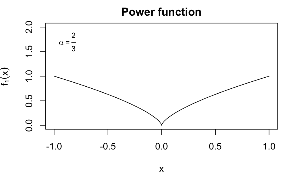
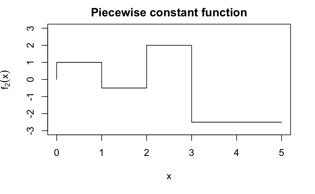
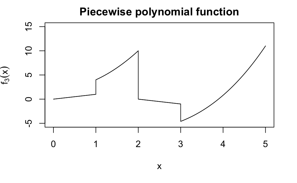
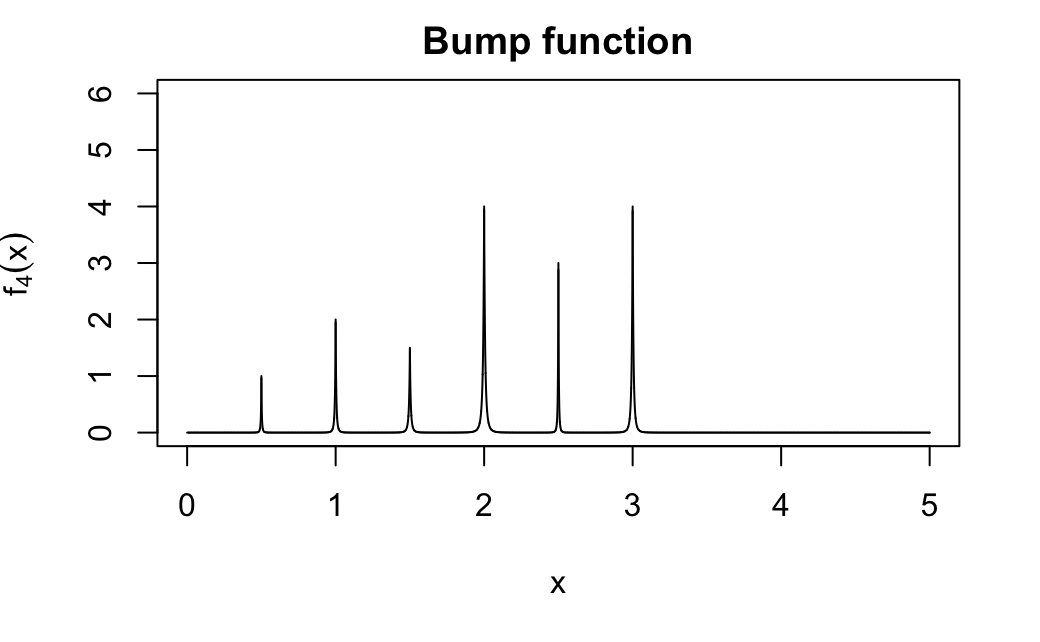
Figure 1: Examples of functions that lie in a Fractional Sobolev spaces. The function $f_{1}$, $f_{2}$, $f_{3}$ and $f_{4}$ are as defined in (7), (8), (9) and (10) respectively.

We end this section by providing some examples of nonsmooth functions that are of interest in nonparametric statistics while not covered by the integer-indexed Sobolev space.

Example 1: Power functions. It has to be noted that the Sobolev space $H^{s}(\mathcal{X})$ for $s\in\mathbb{N}_{+}$ not only requires the functions to be $s$-times (weakly) differentiable but the derivatives have to be square-integrable as well. Let’s consider the following function:

$$f_{1}(x):=|x|^{\alpha},\quad 0<\alpha<1,$$ (7)

on $(-1,1)$. Obviously, $f_{1}$ is not (weakly) differentiable at $0$. Furthermore, note that $\int_{0}^{1}x^{2(\alpha-1)}dx=\infty$, for $0<\alpha\leq 1/2$. Therefore, it doesn’t belong to any integer-indexed Sobolev space when $0<\alpha<1$. However, let us consider

$$|f_{1}|_{H^{s}((-1,1))}=\left(\int_{-1}^{1}\int_{-1}^{1}\frac{||x|^{\alpha}-|y|^{\alpha}|^{2}}{|x-y|^{1+2s}}\,dx\,dy\right)^{1/2},$$

for $0<\alpha<1$ and $0<s<1$. Note that the singularity is at $x=y$. Furthermore, we have $|x|^{\alpha}-|y|^{\alpha}\sim\alpha|y|^{\alpha-1}(x-y)$ as $x\rightarrow y$ for $y\neq 0$ and $\int_{0}^{1}x^{-p}dx<\infty$ for $p<1$. Hence, the fractional Sobolev seminorm $|f_{1}|_{H^{\alpha}((-1,1))}<\infty,$ for $0<s<1$ and $1/2\leq\alpha<1$. In summary, the function hence belongs to the fractional Sobolev space $H^{s}((-1,1))$ for $0<s<1$ when $1/2\leq\alpha<1$.

Example 2. Piecewise constant functions. Now, consider the following function on $[0,1]$:

$$f_{\text{pc}}(x)=\left\{\begin{aligned} &1,\ 0<x\leq 1/2,\\ &0,\ 1/2<x<1.\end{aligned}\right.$$

Clearly, on the same support, $f_{\text{pc}}(x)=f_{\text{pc}}(y)$ for $0<x,y\leq 1/2$ or $1/2<x,y<1$. It then suffices to only consider the following integral:

$$\int_{0}^{\frac{1}{2}}\int_{\frac{1}{2}}^{1}\frac{1}{|x-y|^{1+2s}}\,dx\,dy,$$

for $0<s<1$. As $\int_{0}^{1}x^{-p}dx<\infty$ for $p<1$, it is finite for $0<s<1/2$. Then, the fractional Sobolev seminorm is finite for $0<s<1/2$, which implies $f_{\text{pc}}(x)$ belongs to the fractional Sobolev space $H^{s}([0,1])$ for $0<s<1/2$.

A generalization of the above example is the piecewise constant functions or blocks (see Donoho and Johnstone (1994) for more details) denoted by $f_{2}(x)$, where the function is constant on multiple intervals that form a partition of $\mathcal{X}$. For instance,

$$f_{2}(x)=\left\{\begin{aligned} &1,\quad 0<x\leq 1\\ &0.5,\quad 1<x\leq 2\\ &2,\quad 2<x\leq 3\\ &-2.5,\quad 3<x<5.\\ \end{aligned}\right.$$ (8)

The piecewise constant functions/blocks belong to the fractional Sobolev space $H^{s}(\mathcal{X})$ for $0<s<1/2$.

Example 3. Piecewise polynomial functions. The piecewise polynomial functions extend the blocks above by putting a polynomial function with degree at most $r\geq 0$ on each interval partition of the support $\mathcal{X}$. Furthermore, since we are considering nonsmooth functions, discontinuities at the boundaries of each interval are allowed here. According to the boundedness of the fractional Sobolev seminorms of the power functions $f_{1}(x)$ and the blocks $f_{2}(x)$, the piecewise polynomial functions belong to the fractional Sobolev space $H^{s}(\mathcal{X})$ for $0<s<1/2$ and all $r\in\mathbb{N}$ when $\mathcal{X}$ is considered to be an open, connected and bounded subset of $\mathbb{R}$ (see Section 3.1). For example,

$$f_{3}(x)=\left\{\begin{aligned} &x,\quad 0<x\leq 1\\ &2x^{2}+2,\quad 1<x\leq 2\\ &-x+2,\quad 2<x\leq 3\\ &0.2x^{3}-2x-4,\quad 3<x<5.\\ \end{aligned}\right.$$ (9)

In general dimension $d\geq 1$, the above arguments can be generalized to imply that the piecewise polynomial functions (including the piecewise constant functions) belong to the fractional Sobolev space when each partition of the support $\mathcal{X}$ is connected and bounded and the boundary of each partition is a lower dimensional space, which allows non-axis aligned partitions.

Example 4: Bumps functions The (multiple) bumps are functions that decay fast from each peak of the bumps. In signal processing, the bumps with polynomial decay or exponential decay are commonly considered. For example,

$$f_{4}(x):=\sum_{j=1}^{J}h_{j}K\left(\frac{t-t_{j}}{w_{j}}\right),$$ (10)

where $K(|t|):=(1+|t|)^{-4}$, and $\{t_{j},h_{j},w_{j}\}_{j=1}^{J}$ are parameters that $t_{j}$ are the locations of each peak and $h_{j}$ are the peak values. Due to the polynomial/exponential decay, the bumps $f_{4}(x)$ also belong to the fractional Sobolev space $H^{s}(\mathcal{X})$ for $0<s<1/2$ when $\mathcal{X}$ is considered to be an open, connected and bounded subset of $\mathbb{R}$ (see Section 3.1).

We emphasize that the the nonsmooth functions presented above (including their extensions in $\mathbb{R}^{d}$) are representative of spatially variable functions arising in imaging, spectroscopy and other signal processing applications that are of considerable practical importance. We refer to Donoho and Johnstone (1994); Boudraa et al. (2004); Liu et al. (2016); Sardy et al. (2000, 2001) for additional exposition of the examples.

2.4 Relationship to other function classes

First note that according to the definition of the fractional Sobolev space (i.e., Definition 2.1), bounded Hölder functions of order $\alpha>0$ on bounded domains belong to the fractional Sobolev space for $0<s<(\alpha\wedge 1)$.

Hu et al. (2022) considered nonparametric estimation with general measure-based bounded total variation class, with finite $L_{\infty}$ norms. For this class, they developed minimax estimators. In particular, the total variation norm was with respect to the $L_{1}$ norm of the weak derivatives. Moreover, Fang et al. (2021) investigated a similar class: the bounded variation in the sense of Hardy-Krause. The fractional Sobolev space that we focus on in this work are set to be a subspace of $L_{2}$ space, the corresponding norms are function-value based and do not require weak derivatives to exist. Furthermore, the class of fractional Sobolev spaces can be considered with respect any $L_{p}$ space for $p\geq 1$ (see Di Nezza et al. (2012) for the definition). In general, both bounded variation functional space and fractional Sobolev space can characterise nonsmooth functions. When specializing in the indicator functions, the bounded variation functional space only contains such functions with locally finite perimeter for the support. The exact inclusion relationships between the spaces of bounded variation functions (with respect to the weak derivatives) and $L_{1}$ or $L_{2}$ based fractional Sobolev spaces are not well-explored in the literature, to the best of our knowledge.

Rockova and Rousseau (2021) studied Bayesian estimators when the truth lies in the set of locally Hölder functions with finite $L_{\infty}$ norm. When considering the bounded support $\mathcal{X}$, locally Hölder functions belong to the fractional Sobolev space. However, in general, the Hölder functions include functions that may not even be in $L_{1}$ or $L_{2}$. Imaizumi and Fukumizu (2019) applied deep neural networks to learn a class of nonsmooth functions that are piecewise Hölder. Similar to locally Hölder functions, when considering the bounded support $\mathcal{X}$, bounded piecewise Hölder functions belong to the fractional Sobolev space while in general, the former one allows functions not necessarily in $L_{1}$ or $L_{2}$.

Intuitively speaking, when characterising nonsmooth functions, compared to the aforementioned functional spaces, the fractional Sobolev space tends to allow ‘worse’ local non-smoothness while requiring ‘better’ global smoothness (in $L_{1}$ or $L_{2}$).

3 Theoretical Result

Before stating our assumptions and results, we introduce some conventions. For two real-valued quantities, $A,B$, the notation $A\lesssim B$ means that there exists a constant $C>0$ not depending on $f$, $M$ or $n$ such that $A\leq CB$ and $A\asymp B$ stands for $A\lesssim B$ and $B\lesssim A$. Also, applying the scaled Euclidean norm $\|\cdot\|_{n}$ or the corresponding scaled dot-product $\langle\cdot,\cdot\rangle_{n}$ to a function $f$, is to be understood as applying it to the vector in-sample evaluations $(f(X_{1}),\ldots,f(X_{n}))$ of the function.

3.1 Assumptions

We list the following major assumptions needed for the sampling distribution/density and the kernel $\eta$.

• The distribution $G$ is supported on $\mathcal{X}$, which is an open, connected, and bounded subset of $\mathbb{R}^{d}$ with Lipschitz boundary.

• The distribution $G$ has a density $g$ on $\mathcal{X}$ such that

  $$0<g_{\min}\leq g(x)\leq g_{\max}<\infty,\ \text{for all}\ x\in\mathcal{X},$$

  for some $g_{min},g_{\max}>0$. Additionally, $g$ is Lipschitz on $\mathcal{X}$ with Lipschitz constant $L_{g}>0$.

• The kernel $\eta$ is a non-negative, monotonically non-decreasing function supported on the interval $[0,1]$ and its restriction on $[0,1]$ is Lipschitz and for convenience, we assume $\eta(1/2)>0$ and define

  $$\sigma_{0}:=\int_{\mathbb{R}^{m}}\eta(\|x\|)dx,\ \sigma_{1}:=\frac{1}{d}\int_{\mathbb{R}^{m}}\|y\|^{2}\eta(\|y\|)dy.$$

  Without loss of generality, we will assume $\sigma_{0}=1$ from now on.

Assumptions $(A1)$ and $(A2)$ are mild and standard assumptions on the density function in the field of graph Laplacians, which are also made in Green et al. (2023); Shi et al. (2024); Trillos et al. (2020). Assumption $(A3)$ is a standard normalization condition made on the smoothing kernel; see Trillos et al. (2020) for more details. The requirement that $\eta$ is compactly supported is purely due to our proof technique. While it is in principle possible to generalize it for non-compact kernels as long as the tails decay relatively fast including the Gaussian kernel, that would require obtaining error bounds on extra terms on the tail, which is beyond the scope of this paper.

3.2 Estimation error of PCR-FLE algorithm

Theorem 3.1.

Let Assumptions $(A1)$-$(A3)$ hold, and further assume $f\in H^{s}(\mathcal{X};M)$ for $0<s<1$ and $M>0$. Suppose there exist constants $c_{0},C_{0}>0$ such that

$$c_{0}\left(\frac{\log n}{n}\right)^{\frac{1}{d}} \leq\epsilon\leq C_{0}K^{-\frac{1}{d}},$$

with

$$K=\min\left\{\lfloor(M^{2}n)^{\frac{d}{2s+d}}\rfloor\vee 1,n\right\}.$$ (11)

Then, there exist constants $c,C>0$ not depending on $f,M$ or $n$ such that for $n$ large enough, the estimator $\hat{f}$ defined in (4) satisfies:

$$\|\hat{f}-f\|_{n}^{2}\leq C\big{\{}\big{(}M^{2}(M^{2}n)^{-\frac{2s}{2s+d}}\wedge 1\big{)}\vee{n^{-1}}\big{\}},$$

with probability at least $1-Cn^{2}e^{-cn\epsilon^{d+4}}-Cne^{-cn}-Cne^{-cn\epsilon^{d}}-e^{-K}$.

Remark 3.2.

Theorems 3.1 implies that the PCR-FLE algorithm achieves an upper bound of rates $n^{-2s/(2s+d)}$ with respect to the fractional Sobolev spaces $H^{s}(\mathcal{X})$ for $0<s<1$ with high probability, provided that $n^{-1/2}\lesssim M\lesssim n^{s/d}$. Recall that the minimax optimal rates for the integer-valued Sobolev space $H^{s}(\mathcal{X})$ ($s\in\mathbb{N}_{+}$) is given by $M^{2}(M^{2}n)^{-\frac{2s}{2s+d}}$ in Györfi et al. (2002); Wasserman (2006); Tsybakov (2008). While allowing $s\rightarrow 1^{-}$, it is consistent with the above rates for the first-order Sobolev space $H^{1}(\mathcal{X})$.

Remark 3.3.

Under a fixed-design setup (i.e., a regular lattice/grid), Chatterjee and Goswami (2021) considered optimal regression tree (OPT) and showed that the finite sample risk of ORT is always bounded by $\frac{C(r)k\log N}{N}$ for some constant $C(r)>0$ and $N=c^{d}$ for some grid size $c>0$ when the regression function is piecewise polynomial of degree $r$ on some reasonably regular axis-aligned rectangular partition of the domain with at most $k$ rectangles. While such piecewise polynomial regression function belongs to the fractional Sobolev space, our bound in Theorem 3.1 is valid for a larger family of nonsmooth functions and allows random design set-up.

Remark 3.4.

A phase transition in the fractional Sobolev space $H^{s}(\mathcal{X})$ was discussed in Dunlop et al. (2020, Lemma 4) that the regularity of the fractional Sobolev space depends on $s<d/2$ or $s>d/2$ (when $s<d/2$, $H^{s}(\mathcal{X})$ cannot even embed continuously into the space of continuous functions $C^{0}(\mathcal{X})$). However, it should be noted that Theorem 3.1 does not require the condition $s>d/2$ regardless of the phase transition.

Remark 3.5.

The lower bound for $\epsilon$ makes sure that with this smallest radius, the resulting graph will still be connected with high probability and the upper bound for $\epsilon$ ensures the eigenvalue of the graph Laplacian to be of the same order as its continuum version, the eigenvalue of the Laplacian operator (Weyl’s law). The condition on $K$ is set to trade-off bias and variance.

Remark 3.6.

Antil et al. (2020) considered nonparametric regression via fractional Laplacian regularization. However, no convergence rates of any kind were investigated there. On the other hand, it has been discussed and emphasized in Green et al. (2021, 2023) that Laplacian regularization usually achieves worse minimax rates of convergence especially in high-dimensional space $\mathbb{R}^{d}$ compared to Laplacian eigenmaps.

4 Numerical Experiments

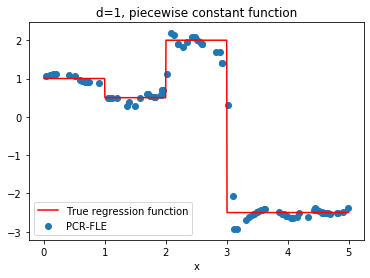
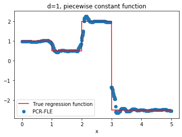
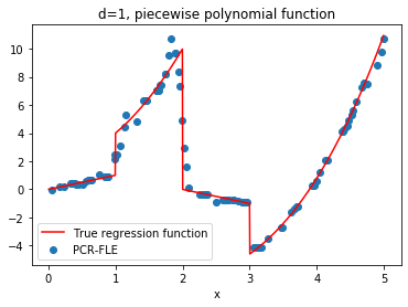
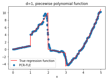
Figure 2: The red line shows the true regression function. The blue line shows the average of the regression fit by PCR-FLE estimation condition on a generation of uniform sample on $[0,5]$: $n=100$ (left) and $n=1000$ (right).

In this section, we empirically demonstrate the performance of the PCR-FLE algorithm in Section 2.2 for learning nonsmooth regression functions. All experiments are done in Python and the codes can be found in the following link:

https://github.com/10Mzys/Fractional_Laplacian_Nonsmooth_Regression/tree/main.

In our experiments, we stick to considering those functions that are of practical importance as introduced in Section 2.3. For simplicity, we set the design distribution $G$ as the uniform distribution and examine the piecewise polynomial (including piecewise constant/the blocks) functions as the true regression function. For the construction of graph Laplacian, we pick a truncated Gaussian kernel. Unless otherwise stated, all tuning parameters are set as the optimal values according to grid search and each experiment is averaged over 200 repetitions.

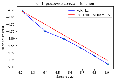
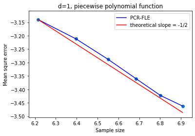
Figure 3: In-sample mean squared error of PCR-FLE as a function of the sample size $n$. Each subplot is on the $\log$-$\log$ scale. The blue line presents the empirical error by PCR-FLE. The red line shows the theoretical upper bound provided by Theorem 3.1 (in slope only and the intercept is set to match the observed error).

We now consider the mean squared error of the PCR-FLE estimation on the nonsmooth functions: the piecewise constant function and the piecewise polynomial function ($f_{2}(x)$ and $f_{3}(x)$ respectively in Figure 1). Due to relatively rapid rate of convergence, the sample size $n$ is set to vary from 500 to 1000. In Figure 2, we present the fitted regression function by PCR-FLE, visually. In Figure 3 ($\log$-$\log$ scale), we show the in-sample mean squared errors of both estimators as a function of the sample size $n$. We see that both estimators have mean squared error converging to 0 roughly at our theoretical rate in Theorem 3.1 while this provides a high probability upper bound.

5 Discussion

We proposed and analyzed the PCR-FLE algorithm for performing nonparametric regression when the true function lies in the $L_{2}$-fractional Sobolev space, $H^{s}(\mathcal{X},M)$. The approach is computational efficient and it involves computing the top-$K$ eigenvalues and eigenvectors of size $n\times n$ graph Laplacian matrix. Under a random design setting, we established rates of convergence of order $n^{-\frac{2s}{2s+d}}$, where $n$ is the number of observations. There are several avenues for future works:

• It is important to establish minimax lower bounds for estimation when the truth lies in fractional Sobolev spaces, under the random design setting, to evaluate worst-case performance of the PCR-FLE algorithm.

• Our current results require knowledge of $s$ and $M$ in setting the bandwidth parameter $\epsilon$ and the number of eigenvalues $K$. It is interesting to develop estimators that are adaptive to the choice of $s$ and $M$, by extending the recent results in Shi et al. (2024).

• It is interesting to go beyond $L_{2}$-fractional Sobolev spaces and consider $L_{1}$-fractional Sobolev spaces which allow for richer class of nonsmooth true functions.

Appendix A Proof of Theorem 3.1

In this section, we will prove Theorem 3.1. To this end, we first present some auxiliary lemmas. In the following, $C$ stands for positive constants that may change from line to line but do not depend on $n$ or $M$.

Lemma A.1 (Weyl’s Law).

Suppose Assumptions (A1) and (A2) hold. There exist constants $c,C>0$ such that

$$ck^{\frac{2}{d}}\leq\Lambda_{k}\leq Ck^{\frac{2}{d}},\quad\text{for all}\ k\geq 1.$$

Here, $\Lambda_{k}$ is the $k$-th eigenvalue of the weighted Laplacian operator $\mathcal{L}_{g}$ in the ascending order, where $\mathcal{L}_{g}u:=-\frac{1}{2g}\text{div}(g^{2}\nabla u)$.

The Weyl’s law is a standard result in operator analysis. We refer interested readers to Dunlop et al. (2020, Lemma 7.10) for a detailed proof.

Lemma A.2 (Lemma 2 in Green et al. (2021)).

There exist constants $C_{1},C_{2},C_{3},C_{4},C_{5}>0$ such that for $n$ large enough and $C_{1}(\log n/n)^{\frac{1}{d}}\leq\epsilon\leq C_{2}$, with probability at least $1-C_{3}ne^{-C_{3}n\epsilon^{d}}$, it holds that

$$C_{4}\left(k^{\frac{2}{d}}\wedge\epsilon^{-2}\right)\leq\lambda_{k}\leq C_{5}\left(k^{\frac{2}{d}}\wedge\epsilon^{-2}\right),\quad\text{for}\ 2\leq k\leq n.$$

The above result actually is different from similar results established in Burago et al. (2015); Trillos et al. (2020); Calder and Trillos (2022), who establish similar results for manifolds without boundary. We refer to Green et al. (2023, Appendix D) for a more detailed discussion.

We are now in the position to prove the main Theorem 3.1.

Proof of Theorem 3.1.

Below, $\mathbb{E}$ denotes the conditional expectation, given $X_{1},\ldots,X_{n}.$ Also recall that the scaled Euclidean norm $\|\cdot\|_{n}$ (or the corresponding dot-product $\langle\cdot,\cdot\rangle_{n}$) applied to a function $f$, means that it is applied to the vector of in-sample evaluations $(f(X_{1}),\ldots,f(X_{n}))$ of the function.

First note that by Cauchy-Schwarz inequality, we have:

$$\|\hat{f}-f\|_{n}^{2}\leq 2(\|\mathbb{E}\hat{f}-f\|_{n}^{2}+\|\hat{f}-\mathbb{E}\hat{f}\|_{n}^{2}).$$

Then, according to PCR-FLE algorithm in Section 2.2, we obtain

$$\|\mathbb{E}\hat{f}-f\|_{n}^{2}=\sum_{k=K+1}^{n}\langle v_{k},f\rangle_{n}^{2}\leq\frac{\langle L_{n,\epsilon}^{s}f,f\rangle_{n}}{\lambda_{K+1}^{s}},$$ (12)

and

$$\|\hat{f}-\mathbb{E}\hat{f}\|_{n}^{2}=\sum_{k=1}^{K}\langle v_{k},\varepsilon\rangle_{n}^{2},$$

where $\varepsilon:=(\varepsilon_{1},\ldots,\varepsilon_{n})^{T}$.

Now, note that if $K=0$, $\hat{f}=0$ then $\|\hat{f}-\mathbb{E}\hat{f}\|_{n}^{2}=0$. We then focus on the case when $K\geq 1$. Since $\langle v_{k},\varepsilon\rangle_{n}$ is normally distributed with $0$ mean and variance

$$\operatorname{Var}\langle v_{k},\varepsilon\rangle_{n}=\frac{1}{n^{2}}\operatorname{Var}\langle v_{k},\varepsilon\rangle=\frac{1}{n},$$ (13)

as $\langle v_{k},v_{k}\rangle=n$. Then, we obtain:

$$\|\hat{f}-\mathbb{E}\hat{f}\|_{n}^{2}=\frac{1}{n}\sum_{k=1}^{K}(\sqrt{n}\langle v_{k},\varepsilon\rangle_{n})^{2}\overset{d}{=}\frac{1}{n}\sum_{k=1}^{K}\mathcal{Z}_{k}^{2},$$

where $\{\mathcal{Z}_{k}\}_{k=1}^{K}$ are i.i.d. standard normal by the orthonormality of the eigenvectors.

According to an exponential concentration inequality for chi-square distributions from Laurent and Massart (2000), we have

$$\mathbb{P}\left(\|\hat{f}-\mathbb{E}\hat{f}\|_{n}^{2}\geq\frac{K}{n}+2\frac{\sqrt{K}}{n}\sqrt{t}+2\frac{t}{n}\right)\leq e^{-t}.$$ (14)

With (12) and (14), it yields that

$$\|\hat{f}-f\|_{n}^{2}\leq\frac{\langle L_{n,\epsilon}^{s}f,f\rangle_{n}}{\lambda_{K+1}^{s}}+\frac{K}{n},$$ (15)

with probability at least $1-e^{-K}$ if $1\leq K\leq n$. Of course, when $K=0$, (15) holds.

Now, it remains to bound the empirical fractional Sobolev seminorm $\langle L_{n,\epsilon}^{s}f,f\rangle_{n}$ and the graph Laplacian eigenvalue $\lambda_{K+1}$ (and its power $\lambda_{K+1}^{s}$) for $0<s<1$. We first focus on the empirical fractional Sobolev seminorm $\langle L_{n,\epsilon}^{s}f,f\rangle_{n}$ for $0<s<1$. Note that Weihs and Thorpe (2023); Dunlop et al. (2020); Trillos and Slepčev (2018) showed $\Gamma$-convergence of the above empirical fractional Sobolev seminorm to its continuum in (5). However, $\Gamma$-convergence does not fully suffice for our purpose. Instead, we will adapt the proof procedures applied in Calder and Trillos (2022); Green et al. (2021, 2023) for our situation, as we describe next.

First note that according to the eigendecomposition of $L_{n,\epsilon}$, we obtain:

$$\langle L_{n,\epsilon}^{s}f,f\rangle_{n}=\sum_{i=1}^{n}\lambda_{i}^{s}\langle f,v_{i}\rangle_{n}^{2},$$ (16)

and by Lemma A.1 and Lemma A.2, we have that

$$\lambda_{i}\lesssim\Lambda_{i},$$

for $1\leq i\leq n$ with probability at least $1-Cne^{-cn\epsilon^{d}}$. We now focus on the eigenvectors $\{v_{i}\}_{i=1}^{n}$. For a given eigenvalue $\Lambda>0$ of $\mathcal{L}_{g}$, assume $\Lambda=\Lambda_{i+1}=\ldots=\Lambda_{i+k}$ for some $i$ and $k$, where $k$ is the multiplicity of $\Lambda$. We then define the eigenvalue gap of $\Lambda$ as:

$$\gamma_{\Lambda}:=\frac{1}{2}\left(|\Lambda-\Lambda_{i}|\wedge|\Lambda-\Lambda_{i+k+1}|\right).$$ (17)

Now, according to Green et al. (2021, Proof of Theorem 5 of Supplementary Material) there exists a constant $A>2$, such that for $\theta,\tilde{\delta}>0$ as defined in Green et al. (2021, Supplementary Material, Equation (A20)) and $\epsilon$ small enough, such that

$$1-A\left(\epsilon\sqrt{\Lambda}+\theta+\tilde{\delta}\right)\geq\frac{1}{2},$$

we have the following: For $\Lambda=\Lambda_{l}$ ($l$-th eigenvalue of $\mathcal{L}_{g}$ in the ascending order) satisfying the above, we have with probability at least $1-Cne^{-cn\theta^{2}\tilde{\delta}^{d}}$,

$$a\lambda_{l}\leq\sigma_{1}\Lambda_{l}\leq A\lambda_{l},$$ (18)

where $a$ is given in Green et al. (2021, Proof of Theorem 5, Supplementary Material) with $a^{-1}\geq 2$. Hence, we have with probability at least $1-Cne^{-cn\theta^{2}\tilde{\delta}^{d}}$, that

$$|\lambda_{l}-\sigma_{1}\Lambda_{l}|\leq((a^{-1}-1)\vee(A-1))\sigma_{1}\Lambda_{l}\leq C\gamma_{\Lambda_{l}}.$$ (19)

Let $S$ be the subspace of $l^{2}$ spanned by the eigenvectors of $L_{n,\epsilon}$ associated to the eigenvalues $\lambda_{i+1},\ldots,\lambda_{i+r}$. In the following, we will establish the bound on the eigenfunctions/eigenvectors of $\Lambda_{j}$ and $\lambda_{j}$ respectively for $j=i+1,\ldots,i+r$. Denote by $P_{S}$ the orthogonal projection (with respect to $\langle\cdot,\cdot\rangle_{n}$) onto $S$ and $P_{S}^{\bot}$ the orthogonal projection onto the orthogonal complement of $S$. Let $h$ be the eigenfunction of $\mathcal{L}_{g}$ corresponding to the eigenvalue $\Lambda$, i.e., $\mathcal{L}_{g}h=\Lambda h$. Considering restriction of $h$ on $X_{1},\ldots,X_{n}$, we have

$$P_{S}^{\bot}\mathcal{L}_{g}h=\Lambda P_{S}^{\bot}h=\Lambda\sum_{j\neq i+1,\ldots,i+r}\langle h,v_{j}\rangle_{n}v_{j},$$

where recall that $\{v_{j}\}_{j=1}^{n}$ are the set of the orthonormal basis of eigenvectors of $L_{n,\epsilon}$ with respect to $\lambda_{1},\ldots,\lambda_{n}$. Similarly, we have (again, restrict $h$ on $X_{1},\ldots,X_{n}$):

$$P_{S}^{\bot}L_{n,\epsilon}h=\sum_{j\neq i+1,\ldots,i+r}\lambda_{j}\langle h,v_{j}\rangle_{n}v_{j}.$$

Combining the two results above, we obtain:

$$\quad\min\{|\sigma_{1}\Lambda-\lambda_{i}|,|\sigma_{1}\Lambda-\lambda_{i+r+1}|\}\|P_{S}^{\bot}h\|_{n}$$

$$\leq\|P_{w,S}^{\bot}(L_{w,n,\epsilon}h-\sigma_{1}\mathcal{L}_{g}h)\|_{n}$$

$$\leq\|L_{n,\epsilon}h-\sigma_{1}\mathcal{L}_{g}h\|_{n},$$

where $\sigma_{1}$ is defined in Section 3.1 (see Assumption (A3)).

On the other hand, according to (17) and (19), we have

$$\min\{|\sigma_{1}\lambda-\lambda_{i}(L_{n,w,\epsilon})|,|\sigma_{1}\lambda-\lambda_{i+r+1}(L_{w,n,\epsilon})|\}\geq\sigma_{1}C\gamma_{\Lambda}.$$

Then, we obtain:

$$\|P_{S}^{\bot}h\|_{n}=\|h-P_{S}h\|_{n}\leq\frac{1}{\sigma_{1}C\gamma_{\Lambda}}\|L_{n,\epsilon}h-\sigma_{1}\mathcal{L}_{g}h\|_{n}.$$ (20)

Now, we divide the above norm $\|\cdot\|_{n}$ into two parts by Cauchy’s inequality:

$$\|L_{n,\epsilon}h-\sigma_{1}\mathcal{L}_{g}h\|_{n}\lesssim\|L_{n,\epsilon}h-\sigma_{1}\mathcal{L}_{g}h\|_{n,\mathcal{X}_{\epsilon}}+\|L_{n,\epsilon}h-\sigma_{1}\mathcal{L}_{g}h\|_{n,\partial\mathcal{X}_{\epsilon}},$$

where we write $\mathcal{X}=\mathcal{X}_{\epsilon}\sqcup\partial\mathcal{X}_{\epsilon}$, where for any $x\in\mathcal{X}_{t\epsilon}$, $B_{x}(\epsilon)\subset\mathcal{X}$ and $\partial_{\epsilon}\mathcal{X}$ as its complement within $\mathcal{X}$ consisting of points ‘close’ to the boundary. According to Calder and Trillos (2022, Theorem 3.3), it follows that if $h_{1},\ldots,h_{k}$ is an orthonormal basis for the eigenspace of eigenfunctions of $\mathcal{L}_{g}$ with respect to eigenvalue $\Lambda$, then with probability at least $1-2kne^{-Cn\epsilon^{d+4}}$,

$$\|L_{n,\epsilon}h_{j}-\sigma_{1}\mathcal{L}_{g}h_{j}\|_{n,\mathcal{X}_{\epsilon}}\leq C\epsilon,\quad 1\leq j\leq k.$$

On the other hand, near the boundary, by setting $k=1$ and $s=3$ (since all $h_{j}$ at least belongs to $C^{3}(\mathcal{X})$) in Green et al. (2023, Lemma 5), it yields that almost surely,

$$\|L_{n,\epsilon}h_{j}\|_{n,\partial\mathcal{X}_{\epsilon}}\leq C\epsilon,\quad 1\leq j\leq k,$$

with $\|\sigma_{1}\mathcal{L}_{g}h_{j}\|_{n,\partial\mathcal{X}_{\epsilon}}\leq C\epsilon$ for $1\leq j\leq$ since all $h_{j}$ at least belongs to $C^{3}(\mathcal{X})$.

Putting the bounds in the interior and near the boundary together, we conclude: with probability at least $1-2kne^{-Cn\epsilon^{d+4}}$,

$$\|L_{n,\epsilon}h_{j}-\sigma_{1}\mathcal{L}_{g}h_{j}\|_{n}\leq C\epsilon,\quad 1\leq j\leq k.$$

Now, combining the above result with (20), it follows that with probability at least $1-2kne^{-Cn\epsilon^{d+4}}-Cne^{-cn\theta^{2}\tilde{\delta}^{d}}$, we can find an orthonormal set $\tilde{h}_{1},\ldots,\tilde{h}_{k}$ of spanning $S$ such that

$$\|h_{j}-\tilde{h}_{j}\|_{n}\leq C\epsilon.$$

Here, recall that $\{h_{j}\}_{j=1}^{k}$ is an orthonormal basis for the eigenspace of eigenfunctions of $\mathcal{L}_{g}$ with respect to eigenvalue $\Lambda=\Lambda_{l}$ and $\{\tilde{h}_{j}\}_{j=1}^{k}$ is an orthonormal set spanning $S$, i.e., the eigenspace of eigenvectors of $L_{n,\epsilon}$ with respect to the eigenvalue $\lambda=\lambda_{l}$. These two sets of functions/vectors are close in $\|\cdot\|_{n}$ norm by $C\epsilon$. Therefore, with $\phi_{i}$ as the projection $i$-th eigenfunction into $\mathbb{R}^{n}$ via the transportation map $\tilde{T}$ defined in Green et al. (2021, Proposition 3), we have: with probability at least $1-2kne^{-Cn\epsilon^{d+4}}-Cne^{-cn\theta^{2}\tilde{\delta}^{d}}$,

$$\|v_{i}-\phi_{i}\|_{n}\leq C\epsilon.$$

Then, plugging the above approximation in (16) with Weihs and Thorpe (2023, Proposition 4.21), we obtain:

$$\langle L_{n,\epsilon}^{s}f,f\rangle_{n} =\sum_{i=1}^{n}\lambda_{i}^{s}\langle f,v_{i}\rangle_{n}^{2}\lesssim\sum_{i=1}^{n}\lambda_{i}^{s}\langle f,v_{i}-\phi_{i}\rangle_{n}^{2}+\sum_{i=1}^{n}\lambda_{i}^{s}\langle f,\phi_{i}\rangle_{n}^{2}$$

$$\lesssim C\left(\epsilon+\sum_{i=1}^{n}\lambda_{i}^{s}\langle f,\phi_{i}\rangle_{n}^{2}\right).$$ (21)

Now recall (5). For $n$ large enough (or equivalently $\epsilon$ small enough) we have

$$\langle L_{n,\epsilon}^{s}f,f\rangle_{n} \lesssim C\sum_{i=1}^{n}\Lambda_{i}^{s}\langle f,\phi_{i}\rangle_{n}^{2}\leq CM^{2}.$$

with probability at least $1-Cn^{2}e^{-Cn\epsilon^{d+4}}-Cne^{-Cn}$, where we have used (18) above.

Furthermore, according to Lemma A.2, we have for $0<s<1$,

$$\left(k^{\frac{2s}{d}}\wedge\epsilon^{-2s}\right)\lesssim\lambda_{k}^{s}\lesssim\left(k^{\frac{2s}{d}}\wedge\epsilon^{-2s}\right),$$ (22)

for $1\leq k\leq n$ (since the case $k=1$ can be bounded alone), with probability at least $1-Cne^{-Cn\epsilon^{d}}$.

Now, we are ready to proceed based on (15):

$$\|\hat{f}-f\|_{n}^{2}\leq\frac{\langle L_{n,\epsilon}^{s}f,f\rangle_{n}}{\lambda_{K+1}^{s}}+\frac{K}{n},$$

with probability at least $1-e^{-K}$ if $1\leq K\leq n$. According to (A) and (22), we have with probability at least $1-Cn^{2}e^{-Cn\epsilon^{d+4}}-Cne^{-Cn}-Cne^{-cn\epsilon^{d}}-e^{-K}$ and $n$ large enough:

$$\|\hat{f}-f\|_{n}^{2}\lesssim\frac{M^{2}}{(K+1)^{2s/d}\wedge\epsilon^{-2s}}+\frac{K}{n}.$$

Furthermore, based on the assumption $\epsilon\lesssim K^{-1/d}$, the above inequality becomes:

$$\|\hat{f}-f\|_{n}^{2}\lesssim M^{2}(K+1)^{-2s/d}+\frac{K}{n}.$$ (23)

The choice $K=\lfloor M^{2}n\rfloor^{d/(2s+d)}$ balances the two terms on the right-hand side, and we obtain

$$\|\hat{f}-f\|_{n}^{2}\lesssim M^{2}(M^{2}n)^{-2s/(2s+d)},$$ (24)

with probability at least $1-Cn^{2}e^{-Cn\epsilon^{d+4}}-Cne^{-Cn}-Cne^{-cn\epsilon^{d}}-e^{-K}$.

If $M^{2}<n^{-1}$, we can take $K=1$ and obtain from (23) that:

$$\|\hat{f}-f\|_{n}^{2}\lesssim\frac{1}{n}.$$

If $M>n^{s/d}$, we take $K=n$ and in this case, we actually have $\hat{f}(X_{i})=Y_{i}$ for $i=1,\ldots,n$ and

$$\|\hat{f}-f\|_{n}^{2}=\frac{1}{n}\sum_{i=1}^{n}\varepsilon_{i}^{2}\lesssim C,$$

with probability at least $1-e^{-n}$ for some constant $C$. Combining all above cases depending on choices of $K$, it yields that bound in Theorem 3.1.

∎

References

- Andreux et al. (2015) Mathieu Andreux, Emanuele Rodolà, Mathieu Aubry, and Daniel Cremers. Anisotropic Laplace-Beltrami Operators for Shape Analysis. In Lourdes Agapito, Michael M. Bronstein, and Carsten Rother, editors, Computer Vision - ECCV 2014 Workshops, Lecture Notes in Computer Science, pages 299–312, 2015.
- Antil et al. (2020) Harbir Antil, Zichao Wendy Di, and Ratna Khatri. Bilevel optimization, deep learning and fractional Laplacian regularization with applications in tomography. Inverse Problems, 36(6):064001, 2020.
- Antil et al. (2021) Harbir Antil, Tyrus Berry, and John Harlim. Fractional diffusion maps. Applied and Computational Harmonic Analysis, 54:145–175, 2021.
- Belkin and Niyogi (2003) Mikhail Belkin and Partha Niyogi. Laplacian eigenmaps for dimensionality reduction and data representation. Neural Computation, 15(6):1373–1396, 2003.
- Belkin and Niyogi (2005) Mikhail Belkin and Partha Niyogi. Towards a theoretical foundation for Laplacian-based manifold methods. In International Conference on Computational Learning Theory, pages 486–500. Springer, 2005.
- Belkin et al. (2006) Mikhail Belkin, Partha Niyogi, and Vikas Sindhwani. Manifold regularization: A geometric framework for learning from labeled and unlabeled examples. Journal of Machine Learning Research, 7(11), 2006.
- Boudraa et al. (2004) AO Boudraa, JC Cexus, and Z Saidi. Emd-based signal noise reduction. International Journal of Signal Processing, 1(1):33–37, 2004.
- Burago et al. (2015) Dmitri Burago, Sergei Ivanov, and Yaroslav Kurylev. A graph discretization of the Laplace–Beltrami operator. Journal of Spectral Theory, 4(4):675–714, 2015.
- Calder and Trillos (2022) Jeff Calder and Nicolás García Trillos. Improved spectral convergence rates for graph Laplacians on -graphs and -NN graphs. Applied and Computational Harmonic Analysis, 60:123–175, 2022.
- Chatterjee and Goswami (2021) Sabyasachi Chatterjee and Subhajit Goswami. Adaptive estimation of multivariate piecewise polynomials and bounded variation functions by optimal decision trees. The Annals of Statistics, 49(5):2531–2551, 2021.
- Chaudhuri et al. (1994) Probal Chaudhuri, Min-Ching Huang, Wei-Yin Loh, and Ruji Yao. Piecewise-polynomial regression trees. Statistica Sinica, pages 143–167, 1994.
- Chun et al. (2016) Yongwan Chun, Daniel A Griffith, Monghyeon Lee, and Parmanand Sinha. Eigenvector selection with stepwise regression techniques to construct eigenvector spatial filters. Journal of Geographical Systems, 18:67–85, 2016.
- Coifman and Lafon (2006) Ronald R Coifman and Stéphane Lafon. Diffusion maps. Applied and Computational Harmonic Analysis, 21(1):5–30, 2006.
- Di Nezza et al. (2012) Eleonora Di Nezza, Giampiero Palatucci, and Enrico Valdinoci. Hitchhiker’s guide to the fractional Sobolev spaces. Bulletin des Sciences Mathématiques, 136(5):521–573, 2012.
- Donoho (1997) David L Donoho. Cart and best-ortho-basis: a connection. The Annals of Statistics, 25(5):1870–1911, 1997.
- Donoho and Johnstone (1994) David L Donoho and Iain M Johnstone. Ideal spatial adaptation by wavelet shrinkage. Biometrika, 81(3):425–455, 1994.
- Dunlop et al. (2020) Matthew M Dunlop, Dejan Slepčev, Andrew M Stuart, and Matthew Thorpe. Large data and zero noise limits of graph-based semi-supervised learning algorithms. Applied and Computational Harmonic Analysis, 49(2):655–697, 2020.
- Dunson et al. (2021) David B Dunson, Hau-Tieng Wu, and Nan Wu. Spectral convergence of graph Laplacian and heat kernel reconstruction in from random samples. Applied and Computational Harmonic Analysis, 55:282–336, 2021.
- Fang et al. (2021) Billy Fang, Adityanand Guntuboyina, and Bodhisattva Sen. Multivariate extensions of isotonic regression and total variation denoising via entire monotonicity and Hardy–Krause variation. The Annals of Statistics, 49(2), 2021.
- Giné and Koltchinskii (2006) Evarist Giné and Vladimir Koltchinskii. Empirical graph Laplacian approximation of Laplace-Beltrami operators: large sample results. Lecture Notes-Monograph Series, pages 238–259, 2006.
- Green et al. (2021) Alden Green, Sivaraman Balakrishnan, and Ryan Tibshirani. Minimax optimal regression over Sobolev spaces via Laplacian regularization on neighborhood graphs. In International Conference on Artificial Intelligence and Statistics, pages 2602–2610. PMLR, 2021.
- Green et al. (2023) Alden Green, Sivaraman Balakrishnan, and Ryan J Tibshirani. Minimax optimal regression over Sobolev spaces via Laplacian Eigenmaps on neighbourhood graphs. Information and Inference: A Journal of the IMA, 12(3):2423–2502, 2023.
- Györfi et al. (2002) László Györfi, Michael Köhler, Adam Krzyzak, and Harro Walk. A distribution-free theory of nonparametric regression, volume 1. Springer, 2002.
- Hacquard et al. (2022) Olympio Hacquard, Krishnakumar Balasubramanian, Gilles Blanchard, Clément Levrard, and Wolfgang Polonik. Topologically penalized regression on manifolds. The Journal of Machine Learning Research, 23(1):7233–7271, 2022.
- Hein et al. (2005) Matthias Hein, Jean-Yves Audibert, and Ulrike von Luxburg. From graphs to manifolds–weak and strong pointwise consistency of graph Laplacians. In International Conference on Computational Learning Theory, pages 470–485. Springer, 2005.
- Hein et al. (2007) Matthias Hein, Jean-Yves Audibert, and Ulrike von Luxburg. Graph laplacians and their convergence on random neighborhood graphs. Journal of Machine Learning Research, 8(6), 2007.
- Hoffmann et al. (2022) Franca Hoffmann, Bamdad Hosseini, Assad A Oberai, and Andrew M Stuart. Spectral analysis of weighted Laplacians arising in data clustering. Applied and Computational Harmonic Analysis, 56:189–249, 2022.
- Hu et al. (2022) Addison J Hu, Alden Green, and Ryan J Tibshirani. The voronoigram: Minimax estimation of bounded variation functions from scattered data. arXiv:2212.14514, 2022.
- Hütter and Rigollet (2016) Jan-Christian Hütter and Philippe Rigollet. Optimal rates for total variation denoising. In Conference on Learning Theory, pages 1115–1146. PMLR, 2016.
- Imaizumi and Fukumizu (2019) Masaaki Imaizumi and Kenji Fukumizu. Deep neural networks learn non-smooth functions effectively. In The 22nd international conference on artificial intelligence and statistics, pages 869–878. PMLR, 2019.
- Koenker and Mizera (2004) Roger Koenker and Ivan Mizera. Penalized triograms: Total variation regularization for bivariate smoothing. Journal of the Royal Statistical Society Series B: Statistical Methodology, 66(1):145–163, 2004.
- Laurent and Massart (2000) Beatrice Laurent and Pascal Massart. Adaptive estimation of a quadratic functional by model selection. Annals of Statistics, pages 1302–1338, 2000.
- Liu et al. (2016) Yuanyuan Liu, Gongliu Yang, Ming Li, and Hongliang Yin. Variational mode decomposition denoising combined the detrended fluctuation analysis. Signal Processing, 125:349–364, 2016.
- Mahadevan and Maggioni (2007) Sridhar Mahadevan and Mauro Maggioni. Proto-value Functions: A Laplacian Framework for Learning Representation and Control in Markov Decision Processes. Journal of Machine Learning Research, 8(10), 2007.
- Mammen and Van De Geer (1997) Enno Mammen and Sara Van De Geer. Locally adaptive regression splines. The Annals of Statistics, 25(1):387–413, 1997.
- Ng et al. (2001) Andrew Y. Ng, Michael I. Jordan, and Yair Weiss. On Spectral Clustering: Analysis and an Algorithm. In Neural Information Processing Systems: Natural and Synthetic, NIPS’01, pages 849–856, January 2001.
- Rice (1984) John Rice. Bandwidth choice for nonparametric regression. The Annals of Statistics, pages 1215–1230, 1984.