Optimizing Language Models for Human Preferences
 is a Causal Inference Problem

Abstract

As large language models (LLMs) see greater use in academic and commercial settings, there is increasing interest in methods that allow language models to generate texts aligned with human preferences. In this paper, we present an initial exploration of language model optimization for human preferences from direct outcome datasets, where each sample consists of a text and an associated numerical outcome measuring the reader’s response. We first propose that language model optimization should be viewed as a causal problem to ensure that the model correctly learns the relationship between the text and the outcome. We formalize this causal language optimization problem, and we develop a method—causal preference optimization (CPO)—that solves an unbiased surrogate objective for the problem. We further extend CPO with doubly robust CPO (DR-CPO), which reduces the variance of the surrogate objective while retaining provably strong guarantees on bias. Finally, we empirically demonstrate the effectiveness of (DR-)CPO in optimizing state-of-the-art LLMs for human preferences on direct outcome data, and we validate the robustness of DR-CPO under difficult confounding conditions.

1 Introduction

Recent advances in computation have yielded large-scale self-supervised language models that achieve impressive performance on a variety of natural language processing (NLP) tasks [Zhang et al., 2022, Chowdhery et al., 2023, Scao et al., 2023, Bubeck et al., 2023]. These large language models (LLMs)—trained on vast amounts of text data of varying quality—can acquire less desirable attributes from these texts, and so they often require further fine-tuning on human preferences to improve their factual correctness and alignment with social values (e.g., less toxic, more helpful) [Ouyang et al., 2022, Bommasani et al., 2022].

In this paper, we examine a paradigm for language model optimization for human preferences that has previously been underexplored: learning from direct outcome datasets, which are ubiquitous in NLP. In contrast to paired completion data consisting of prompts followed by one preferred and one non-preferred completion, direct outcome datasets are text datasets where each sample consists of a text and an associated numerical outcome measuring the reader’s response to the text (e.g., Reddit upvotes [Lakkaraju et al., 2021], Amazon ratings [McAuley and Leskovec, 2013]). A large number of direct outcome datasets are crowdsourced datasets, where annotators on a crowdsourcing platform are randomly assigned to read and respond to texts.

The ability to learn human preferences from direct outcome data significantly broadens the scope of problems that can be addressed by learning from human feedback. Consider the task of inducing a language model to unlearn hate speech. Current unlearning approaches typically use paired data in the format ([hate speech], [alternative text]), with the preferred text being the latter. Constructing alternative texts can be difficult [Eldan and Russinovich, 2023, Maini et al., 2024], and rather than fully unlearning the hate speech, the language model is instead trained to preferentially generate the alternative text [Patil et al., 2024]. Direct outcome data, by contrast, allows texts to be directly marked as hateful and removed from the language model without learning or requiring an alternative text.

We present an initial exploration of language model optimization in the direct outcome setting, where the language model is fine-tuned to optimize texts with respect to a desired outcome. We first note that learning an optimal language model can be difficult due to the presence of unmeasured confounding in the training data: external factors that affect both readers’ choice of texts to read and how they tend to respond to those texts. Language models optimized on confounded data may learn incorrect relationships between texts and reader responses, leading them to generate sub-optimal text. For instance, users of hate speech are both (i) more likely to engage with content containing hate speech and (ii) more likely to rate hateful content positively. Such confounding may lead to incomplete unlearning of hate speech, as some examples of hate speech are assigned positive outcomes in the confounded data.

Therefore, we posit that language model optimization should be viewed as a causal problem in order to ensure that the optimal language model causes preferred outcomes. In this paper, we introduce a causal formulation of the language model optimization problem. The solution to this optimization problem finds how to intervene on the text distribution of the generating model to best cause an optimal outcome (i.e., generation of human-preferred texts).

We observe that in the direct outcome setting, it is possible in practice to guarantee that the observed relationship between the text and the outcome is causal by leveraging crowdsourced datasets. Due to random assignment of texts to readers, crowdsourced datasets are not subject to external confounding and can in fact be viewed as randomized experiments [Lin et al., 2023]. Building on this observation, we present two methodological contributions that enable causal language model optimization on direct outcome datasets. First, we develop causal preference optimization (CPO), which solves an unbiased surrogate objective for the causal optimization problem. Next, we extend this to doubly robust CPO (DR-CPO), which improves on CPO by reducing the variance of the surrogate objective via outcome modeling while retaining provably strong guarantees on bias.

We empirically assess the effectiveness of (DR-)CPO in optimizing state-of-the-art LLMs for human preferences on direct outcome data, both with and without confounding. We find that CPO methods successfully optimize LLMs for human preferences and outperform baselines, and we further observe empirical evidence for the robustness of DR-CPO under difficult confounding conditions.

2 Related Work

2.1 Language Model Optimization

The performance of large self-supervised language models can be further improved by fine-tuning on datasets that align them with human-preferred text [Ouyang et al., 2022, Bommasani et al., 2022]. These paired completion datasets typically consist of prompts followed by two candidate completions, one of which is indicated to be human-preferred [Ethayarajh et al., 2022, Bai et al., 2022, Ji et al., 2023]. A reinforcement learning algorithm may then derive its reward model from these datasets (reinforcement learning from human feedback, or RLHF) [Christiano et al., 2017], after which language models are fine-tuned to maximize the human preference reward under the RLHF algorithm.

While RLHF has seen widespread use [Stiennon et al., 2020, Touvron et al., 2023], it is computationally demanding, as its training loop requires that new texts be generated and new rewards be computed at each step. Consequently, in recent months, methods that allow language models to learn more directly from human preference data have emerged [Hejna et al., 2023, Dumoulin et al., 2024]—the most popular of which is direct preference optimization (DPO) [Rafailov et al., 2023]. Like RLHF, DPO is designed for use with paired completion datasets, maximizing the probability ratio of preferred completions to non-preferred completions over the paired completion dataset.

2.2 Causal Inference and Doubly Robust Policy Learning

Although RLHF and DPO constitute the two most popular optimization approaches for language models, there exists a wide body of work on estimation and policy learning outside of the NLP space. Some notable work relevant to this paper includes a long history of doubly robust estimation of causal effects [Robins et al., 1994] and—more directly applicably—doubly robust policy learning [Dudík et al., 2011, Jiang and Li, 2016, Tang et al., 2020, Athey and Wager, 2021, Kallus et al., 2022].

In causal inference, double robustness denotes an estimator formulation that provides robustness against misspecification of nuisance parameters or functions. In particular, doubly robust estimators combine two existing estimators—an importance weighting estimator and an outcome modeling estimator—such that only one of the two components must be correctly specified or estimated to guarantee the unbiasedness of the estimator [Robins et al., 1994, Chernozhukov et al., 2022]. This can also be viewed as the importance weighting term providing a bias correction for the outcome modeling term. The principle of double robustness can be extended to not only the estimation of causal effects but also the estimation of any quantity, including loss functions or policy objectives, as we do here.

3 A Causal View of Language Model Optimization

When a language model $f$ is trained or fine-tuned to generate texts that are consistent with human preferences, the implicit goal can be seen as optimizing texts $X\sim P^{f}$—texts generated from the model $f$—with respect to some outcome $Y$. In this paper, we consider a direct outcome data format $\mathcal{D}_{O}=\{(X_{1},Y_{1}),\dots,(X_{n},Y_{n})\}$, where $X_{i}$ is a text that individual $i$ interacts with and $Y_{i}$ is any numerical response of the individual to the texts (e.g., ratings, either binary or scalar).

An association-based approach to optimize model $f$ is to generate texts that are similar to those that have high outcomes in the dataset, i.e.,

$$\underset{f}{\arg\max}\;\mathbb{E}_{X\sim P^{f}}[E_{\mathcal{D}_{O}}[Y|X]],$$ (1)

where the conditional expectation $\mathbb{E}_{\mathcal{D}_{O}}[Y|X]$ is the average outcome among individuals who observed the text $X$ and can be learned from $\mathcal{D}_{0}$. A language model optimized under Equation (1) will generate texts that are correlated with high outcomes. We distinguish this from our true optimization goal: to learn—across all possible texts and outcomes—to intervene on the distribution of the generating language model to cause the best possible outcomes.

These hypothetical outcomes can be formalized using the potential outcomes framework [Neyman, 1923 [1990], Rubin, 1974]: over text space $\mathcal{X}$, for each individual $i$ we posit the existence of a potential outcome function $Y_{i}:\mathcal{X}\to\mathbbm{R}$, where $Y_{i}(x)$ encodes their potential real-valued response if given text $x$. We emphasize that most individuals’ potential outcomes are not observed, and so $Y_{i}(x)$ denotes the response individual $i$ would have had had they seen text $x$, possibly contrary to reality. This is also commonly known as the counterfactual.

We assume that we sample individuals from a population $\mathcal{G}$ so that the set of potential outcomes is given by $\{Y(x)\;|\;x\in\mathcal{X}\}\sim\mathcal{G}$. We define $g(x)\equiv\mathbb{E}_{Y(\cdot)\sim\mathcal{G}}[Y(x)]$ as the average outcome if all individuals in the population were given text $x$. Note that $g(x)$ is different from the correlational measure $\mathbb{E}_{\mathcal{D}_{O}}[Y|X]$ because for $\mathbb{E}_{\mathcal{D}_{O}}[Y|X]$, the association between $X$ and $Y$ may be confounded by an external factor.

Formally, then, our goal is to find a language model $f$ that causes high outcomes $Y$ on average across the population of individuals $\mathcal{G}$ and across the texts generated according to the model. We encode the quality of a generative text model $f$ via its value function that measures the expected outcome (or reward):

$$V(f)\equiv\mathbb{E}_{X\sim P^{f}}[\mathbb{E}_{Y(\cdot)\sim\mathcal{G}}[Y(X)]]=\mathbb{E}_{X\sim P^{f}}[g(X)]$$ (2)

Then the causal optimization problem is to find the language model $f$ that maximizes the expected outcome if a random individual were given a random text according to $P^{f}$:

$$\underset{f}{\arg\max}\;V(f)=\underset{f}{\arg\max}\;\mathbb{E}_{X\sim P^{f}}[\mathbb{E}_{Y(\cdot)\sim\mathcal{G}}[Y(X)]]$$ (3)

In intuitive terms, this optimization problem asks the following question: which texts would we generate if we knew what every individual’s response to every text would be? By optimizing the text with respect to every possible response, this construction removes confounding influences on which texts are read or observed, such that the content of the text must be the sole factor that causes the outcome.

4 (Doubly Robust) Causal Preference Optimization

Reframing our optimization problem as a causal inference problem allows us to draw on solutions from statistical causal inference—in particular, the use of randomized experiments to identify causal effects and approximate observing all potential outcomes. We formalize such a randomized experiment and/or crowdsourced annotated dataset as $\mathcal{D}_{R}=\{(X_{1},Y_{1}),\ldots,(X_{n},Y_{n})\}$ where texts $X_{i}$ are drawn i.i.d. from a randomization distribution $P^{R}$ and individuals with potential outcome functions $Y_{i}(\cdot)$ are drawn i.i.d. from the population $\mathcal{G}$. This induces a distribution on the observed responses $Y_{i}=Y_{i}(X_{i})$ that we denote as $P^{R}_{y}$.

Random assignment of individuals to texts removes all confounding outside of the text, since no external factors influence which texts the individual reads. Formally, we have that the texts are independent of the full set of potential outcomes, i.e., $\{Y(x)\mid x\in\mathcal{X}\}\perp\!\!\!\!\perp X$. We also require a technical assumption that there is overlap between the randomization distribution $P^{R}$ and the distribution $P^{f}$ generated by the language model we are optimizing: that is, if $P^{R}(x)=0$, then $P^{f}(X)=0$ as well. This ensures that the randomization distribution is sufficiently informative about the domain we want to optimize over. In principle, this is directly enforceable as a constraint on the language model. In practice, due to the underlying structure of text data and the fact that we often fine-tune language models to the text domain as a precursor to optimization, the overlap assumption is unlikely to be binding.

In this section, we describe causal preference optimization (CPO), which solves an unbiased surrogate objective for the true causal optimization problem using importance weighting. Following this definition, we extend CPO using the principle of double robustness, in which we use outcome modeling to reduce the variance of the CPO objective while retaining strong guarantees on bias.

Derivations and technical results are shown in Appendix A.

4.1 Causal Preference Optimization

Identification. The value of the language model $V(f)$ is a causal quantity that involves the potential outcomes for all individuals, some of which are unobserved. However, we can link the value function to the randomization dataset $\mathcal{D}_{R}$ (i.e., identify it from the observed data) by writing in the following way.

Proposition 4.1.

The value function $V(f)$ can be identified as

$$V(f) =\mathbb{E}_{X\sim P^{R}}\Bigg{[}\mathbb{E}_{Y\sim P^{R}_{y}}\Bigg{[}\frac{P^{f}(X)}{P^{R}(X)}Y\Bigg{]}\Bigg{]} V_{IPW}$$ ()

This value function draws on importance weighting principles from statistical causal inference (also referred to as IPW). Observed outcomes $Y\sim P^{R}_{y}$ are weighted by the density ratios between texts drawn from the language model $X\sim P^{f}$ and texts drawn from the randomization distribution $X\sim P^{R}$; this approximates the average outcome under $P^{f}$, which is not observed.

Estimation. After writing the causal quantity $V(f)$ in terms of observable data, we focus on estimating $V(f)$ in practice. The importance weighting value function $V_{IPW}(f)$ can be estimated directly from the crowdsourced data $\mathcal{D}_{R}$ as follows (recall that $X_{i}\sim P^{R},Y_{i}\sim P^{R}_{y}$):

$$\widehat{V}_{IPW}(f)=\frac{1}{n}\sum_{i=1}^{n}\frac{P^{f}(X_{i})}{P^{R}(X_{i})}Y_{i}$$

Note that both $P^{f}$ and $P^{R}$ are known quantities and do not need to be estimated—$P^{f}$ because it is obtained directly from the model $f$ we are optimizing, and $P^{R}$ because we know the randomization mechanism of the texts in $\mathcal{D}_{R}$. Importantly, this means that $\widehat{V}_{IPW}(f)$ is an unbiased estimator for $V(f)$.

Theorem 4.2.

Let $\mathcal{D}_{R}$ be a randomized experiment parameterized by $P^{R}$, such that $P^{R}$ is known. Then

$$\mathbb{E}_{Y(\cdot)\sim\mathcal{G}}[\mathbb{E}_{X}[\widehat{V}_{IPW}(f)]] =\mathbb{E}_{X\sim P^{f}}[\mathbb{E}_{Y(\cdot)\sim\mathcal{G}}[Y(X)]]$$

$$=V(f)$$

4.2 Doubly Robust Causal Preference Optimization

An importance weighting estimator like the CPO value function is a natural solution for estimating causal quantities when randomized experimental data such as crowdsourced data is available. However, CPO optimizes over only the experimental data, and so it can be further improved by the addition of an outcome modeling term that predicts outcomes on unlabeled texts. The combination of IPW and outcome modeling yields a doubly robust estimator (DR-CPO) that reduces the variance of CPO and improves its generality while still remaining unbiased for the true causal optimization problem.

Identification. The doubly robust formulation gives us another way of linking the value function to the randomization dataset $\mathcal{D}_{R}$.

Proposition 4.3.

The value function $V(f)$ can also be identified as

$$V(f)= \;\mathbb{E}_{X\sim P^{R}}\Bigg{[}\mathbb{E}_{Y\sim P^{R}_{y}}\Bigg{[}\frac{P^{f}(X)}{P^{R}(X)}(Y-g(X))\Bigg{]}\Bigg{]}+$$

$$\;\mathbb{E}_{X\sim P^{f}}[g(X)] V_{DR}$$ ()

This construction combines IPW and an outcome model $g$ to provide robustness against misspecification or mis-estimation within either term—akin to doubly robust estimators that serve the same purpose when estimating causal effects.

Estimation. The doubly robust value function $V_{DR}$ can be estimated from the crowdsourced data $\mathcal{D}_{R}$ and a learned outcome model $\widehat{g}(X)$.

First, however, we consider the outcome modeling term $\mathbb{E}_{X\sim P^{f}}[g(X)]$. Even if we were to have access to the true outcome model $g$, it is difficult to optimize $g$ with respect to texts $X\sim P^{f}$, as this requires that texts be drawn from the language model $f$ as $f$ is being updated. To remedy this, we re-write $\mathbb{E}_{X\sim P^{f}}[g(X)]$ in terms of a fixed language model $f^{0}$:

$$\mathbb{E}_{X\sim P^{f}}[g(X)]=\mathbb{E}_{X\sim P^{f^{0}}}\Bigg{[}\frac{P^{f}(X)}{P^{f^{0}}(X)}g(X)\Bigg{]} V_{out}$$ ()

where $P^{f_{0}}$ denotes the distribution over texts from language model $f_{0}$.

We can create a Monte Carlo estimate of this by drawing texts $\widetilde{X}_{1},\ldots,\widetilde{X}_{m}\sim P^{f^{0}}$ and computing

$$\widehat{V}_{out}(f)=\frac{1}{m}\sum_{j=1}^{m}\frac{P^{f}(\widetilde{X}_{j})}{P^{f^{0}}(\widetilde{X}_{j})}\widehat{g}(\widetilde{X}_{j})$$

where $\widehat{g}(x)$ is a model trained to predict $Y$ from $X$ and $f^{0}$ is any generative language model.

Finally, the doubly robust value function $V_{DR}$ can be estimated as a combination of these two terms.

$$\widehat{V}_{DR}(f)= \;\frac{1}{n}\sum_{i=1}^{n}\frac{P^{f}(X_{i})}{P^{R}(X_{i})}(Y_{i}-\widehat{g}(X_{i}))+$$

$$\;\frac{1}{m}\sum_{j=1}^{m}\frac{P^{f}(\widetilde{X}_{j})}{P^{f^{0}}(\widetilde{X}_{j})}\widehat{g}(\widetilde{X}_{j})$$

Formally, it can be shown that $\widehat{V}_{DR}(f)$ is an unbiased estimator for $V(f)$ under two possible conditions, making it an effective proxy for the true causal optimization problem.

Theorem 4.4.

Let $\mathcal{D}_{R}$ be a randomized experiment parameterized by $P^{R}$, which may be estimated from a separate sample by $\widehat{P}^{R}$. Let $g(X)=E_{Y(\cdot)\sim\mathcal{G}}[Y(X)]$, which may be estimated from a separate sample by $\widehat{g}(X)$. Then

$$\mathbb{E}_{Y(\cdot)\sim\mathcal{G}}[\mathbb{E}_{X}[\widehat{V}_{DR}(f)]] =\mathbb{E}_{X\sim P^{f}}[\mathbb{E}_{Y(\cdot)\sim\mathcal{G}}[Y(X)]]$$

$$=V(f)$$

if either

1. $\widehat{P}^{R}(X)=P^{R}(X)$, or

2. $\widehat{g}(X)=g(X)$

Importantly, because $P^{R}$ is known in randomized experiments, including the crowdsourced data setting, it does not need to be estimated, which means that condition (1) is always fulfilled for DR-CPO. Therefore, $\widehat{V}_{DR}(f)$ is guaranteed to be unbiased for $V_{DR}$ even if the outcome model is incorrect. In other words, DR-CPO is robust to misspecification of $\widehat{g}$, as the IPW term in its value function corrects for any bias from the predicted outcomes.

As a result, rather than learning only from the experimental data $X\sim P^{R},Y\sim P^{R}_{y}$, a model optimized with DR-CPO will additionally be able to leverage the generative language model $f^{0}$ to learn from unlimited unlabeled text $\widetilde{X}\sim P^{f^{0}}$ with predicted outcomes $\widehat{g}(\widetilde{X})$. This can reduce the variance of the value function estimator.

Proposition 4.5.

If $\widehat{g}$ is fit on a separate sample, then conditional on $\widehat{g}$, $n\left(\text{Var}\left(\widehat{V}_{IPW}(f)\right)-\text{Var}\left(\widehat{V}_{DR}(f)\right)\right)$ is equal to

$$\text{Var}\left(\frac{P^{f}(X)}{P^{R}(X)}g(X)\right)-\text{Var}\left(\frac{P^{f}(X)}{P^{R}(X)}\left(g(X)-\widehat{g}(X)\right)\right)$$

$$\quad-\frac{n}{m}\text{Var}\left(\frac{P^{f}(\widetilde{X})}{P^{f^{0}}(\widetilde{X})}\widehat{g}(\widetilde{X})\right)$$

Proposition 4.5 shows the difference in the variances of the IPW and DR value function estimators, scaled by the sample size $n$ of the crowdsourced data to highlight asymptotic differences. This difference indicates that $\text{Var}(\widehat{V}_{DR}(f))<\text{Var}(\widehat{V}_{IPW}(f))$ subject to two conditions: (i) the number of Monte Carlo samples drawn from $f^{0}$ is much larger than the sample size of the crowdsourced data, i.e., $m\gg n$; and (ii) $\widehat{g}(x)$ has some additional predictive power compared to a constant model.

Condition (i) limits the component of the variance difference that arises due to Monte Carlo error from taking $m$ samples from the reference language model $f^{0}$. Then the main comparison is the difference between the variance of the expected outcome $g(x)$, and the variance of the prediction error for the model. As a result, under condition (ii), we can expect the variance of $\widehat{V}_{DR}$ to be lower than the variance of $\widehat{V}_{IPW}$ (e.g., if $(\widehat{g}(x)-g(x))^{2}<g(x)^{2}$).

We note that in a different data setting where the true $P^{R}$ is unknown, a well-estimated $\widehat{g}$ that is close to the true $g$ can also help bias-correct any mis-estimation of $\widehat{P}^{R}(X)$. This may occur, for instance, when no text experiment or crowdsourced dataset is available, but a large amount of clean data exists to train the outcome model.

4.3 Relationship to Existing Approaches

Elements of (DR-)CPO are reflected in two of the most prominent existing language model optimization approaches: RLHF and DPO.

First, notice that the outcome modeling term $V_{out}$ is itself a way of identifying $V(f)$ from the observed data. Outcome modeling relies entirely on the predictive model $\widehat{g}$ and unlabeled texts $\widetilde{X}\sim P^{f^{0}}$ and therefore does not require an experimental dataset $\mathcal{D}_{R}$. However, if $\widehat{g}(X)$ is not a good outcome model, then $\widehat{V}_{out}(f)$ will be biased with respect to $V(f)$. In particular, reward models trained on confounded data may be misspecified, since they can only capture the relationship between the text and the response—and not the confounders that have additionally influenced the response. While these issues are remedied if the confounding is also fully modeled, confounders are extremely difficult to measure fully in text data.

Optimization of $V_{out}(f)$ is closely related to RLHF via proximal policy optimization (PPO) in the direct outcome data setting. In particular, the PPO policy loss term can be seen as a version of outcome modeling in which the reward model is trained on paired completion data. Under these conditions, the RLHF reward model is analogous to the outcome model $g$, and the RLHF policy loss is mathematically equivalent to $V_{out}(f)$ (details in Appendix B).

Likewise, DPO shares similarities with CPO. Both DPO and CPO fine-tune a language model for human feedback by directly using a preference dataset rather than relying on reward or outcome modeling. The DPO objective is similar to $V_{IPW}$ in that it directly increases the likelihood of texts corresponding to desired outcomes through importance weighting. However, because of the paired nature of the data, DPO increases the density ratio between preferred and non-preferred examples, while CPO directly increases the probability of texts with desired outcomes and decreases the probability of texts with non-desired outcomes. Given a paired data setting, the DPO objective could possibly be recovered from $V_{IPW}$; we leave this derivation for future work.

5 Experiments

We conduct evaluations to empirically assess the effectiveness of CPO and DR-CPO in optimizing language models for human preferences on direct outcome data, and we examine the doubly robust properties of DR-CPO under confounding.

5.1 Datasets

To evaluate optimization on direct outcome data, we consider three crowdsourced or randomized experimental datasets in which human annotators provided numerical responses to texts.

Hate Speech (binary outcome). The Hate Speech dataset [Qian et al., 2019] consists of comments from the social media sites Reddit and Gab. Outcomes are collected via crowdsourcing and indicate whether the annotator percieves the comment to be hate speech. The Reddit comments are chosen from subreddits where hate speech is more common, and Gab is a platform where users sometimes migrate after being blocked from other social media sites. The optimization goal for this dataset is to generate texts that are less hateful on average.

Hong Kong (scalar outcome). The Hong Kong dataset [Fong and Grimmer, 2021] consists of texts concerning the Hong Kong democracy protests of 2019-2020. These texts are loosely based on speeches made about Hong Kong during U.S. Congressional sessions at the time of the protests. Outcomes are collected via a randomized experiment and indicate on a scale of 0-100 to what extent the respondent thinks that the U.S. should support Hong Kong during this time, after reading the text. The texts are programmatically constructed: for each text, 2 or 3 text attributes are randomly chosen out of 7 (e.g., commitment, bravery, mistreatment). Short passages corresponding to each attribute are then randomly chosen from a pool of about 20 to construct the text. The optimization goal for this dataset is to generate texts with high outcomes on average.

Confounded (scalar outcome). The Confounded dataset is a version of the Hong Kong dataset where we have induced confounding. We consider the strongest possible form of confounding: the confounder is fully correlated with the outcome, resulting in all outcomes being negations of the original outcomes. This dataset is used to train outcome models. We include this dataset with the realistic expectation that text data is often confounded, which poses a threat to outcome model-based approaches. Therefore, it is necessary to evaluate how different optimization approaches fare under confounding. Like the Hong Kong dataset, the optimization goal for this dataset is to generate texts with high outcomes on average.

5.2 Implementation

Evaluation. To evaluate how well optimization for human preferences has occurred, we use a text preference framework in which a reader is asked to choose the better (with respect to the outcome) of a pair of texts generated by two different methods. Using GPT-4 as a proxy for human annotators, we compare pairs of (method, baseline) completions for the same prompt; across all pairs, we compute method win rates and compute 95% confidence intervals. Since the datasets used for these experiments contain one text per sample rather than a prompt and a completion, we create prompts on the evaluation set by truncating each text to a random length.

The full input provided to GPT-4 for each dataset can be found in Appendix C.1. We validate the use of GPT-4 as an annotator with a human study, which we describe in further detail in Section 6.1.

Methods. We evaluate language models optimized using CPO and DR-CPO. As our baselines, we consider language models that have been fine-tuned on texts from each of the task datasets (FT), as well as models optimized using the outcome modeling value function $V_{out}(f)$. Since—as we discuss in Section 4.3—the $V_{out}(f)$ objective is mathematically equivalent to the RLHF objective, we refer to this baseline as OO-RLHF (offline outcome RLHF).

We use Llama 2 7B [Touvron et al., 2023] as our base language model and fine-tune with low-rank adaptation [Hu et al., 2022]. All optimizations are applied after fine-tuning on text from the task dataset.

Choice of $f^{0}$. When optimizing with DR-CPO or OO-RLHF, any generative language model may be used as $f^{0}$, the fixed language model from which texts are drawn as input to the outcome model. One key consideration is whether $f^{0}$ should be a pre-trained model or whether it should be a model that has been fine-tuned on text relevant to the task—for instance, the randomized experiment dataset $\mathcal{D}_{R}$.

In practice, we choose a pre-trained model as $f^{0}$ to leverage the diversity of texts such models tend to generate. If $\widehat{g}(X)$ is a good outcome model, then predicted outcomes on these texts will still be close to the true outcomes, and DR-CPO and OO-RLHF will benefit from outcome modeling.

Choice of $\widehat{P}^{R}$. In Section 4.1, we mention briefly that although the distribution of texts $P^{R}(X)$ under the randomized experiment is known, it can be helpful empirically to instead compute an estimated $\widehat{P}^{R}(X)$. This is generally due to the fact that the sample probability of each text $X$ may not actually be equal to its theoretical probability merely by chance [Hájek, 1971, Särndal et al., 2003].

We find this to be the case in our experiments, and so we use $\widehat{P}^{R}(X)$ estimated from a Llama 2 7B model fine-tuned on $\mathcal{D}_{R}$ in our CPO and DR-CPO implementations.

6 Results and Discussion

6.1 GPT-4 Annotation Validity

Annotator 1	Annotator 2	Fleiss’ $\kappa$
Human	Human	0.170
Human	GPT-4	0.219
Human majority	GPT-4	0.192

Table 1: Agreement rates of human annotators and GPT-4 when asked to choose preferred texts with respect to target outcomes. We examine inter-human agreement, human-GPT-4 agreement, and agreement between a majority vote of human annotators and GPT-4.

Following the precedent set by Rafailov et al. [2023], we conduct a human study to assess the validity of GPT-4 as an annotator when choosing between pairs of texts for a preferred outcome. Across 200 randomly sampled examples from the Hong Kong dataset, we show human annotators (method, baseline) completion pairs and ask them to choose the better of the two with respect to the outcome. We compute agreement between each human annotator, as well as agreement between each human annotator and GPT-4. Agreement is measured through Fleiss’ $\kappa$ [Fleiss, 1971], a common metric for agreement among multiple raters.

We use the online research platform Prolific to conduct our human study. To avoid annotator fatigue, examples are annotated in batches of 20. We recruit a total of 30 annotators for an average of 3 annotators per example and a total of 600 annotations.

Across three comparisons—human-human, majority vote-human, and human-GPT-4—we find that GPT-4 exhibits a similar or better level of agreement with human annotators as human annotators do with each other (Table 1). We conclude that GPT-4 is a reasonable surrogate for human annotators.

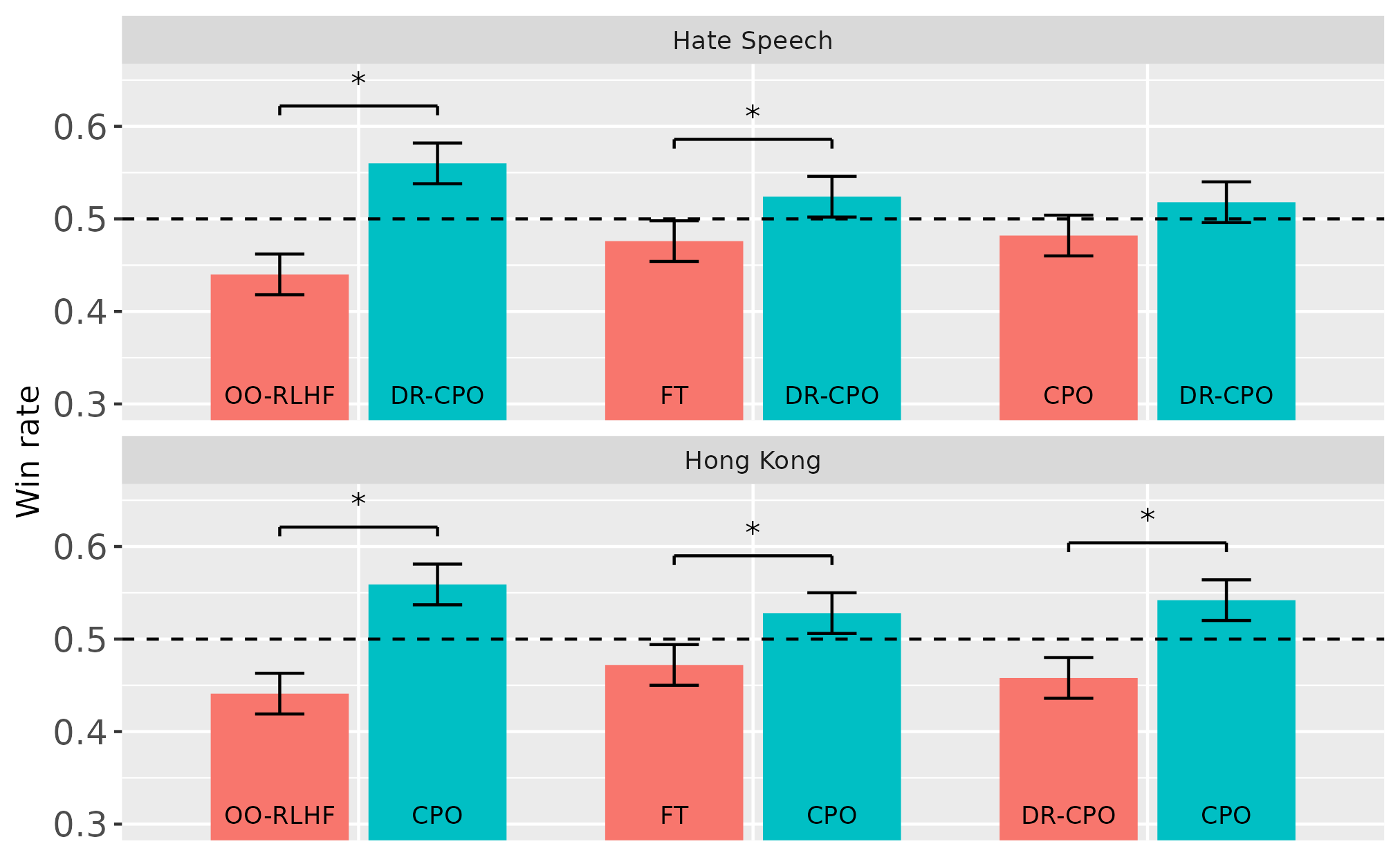
Figure 1: CPO and DR-CPO win rates against OO-RLHF, FT, and each other. A win rate exceeding 0.5 indicates that the named method outperforms the competing method with respect to the target outcome. Win rates are computed across 2000 pairs for each method combination.

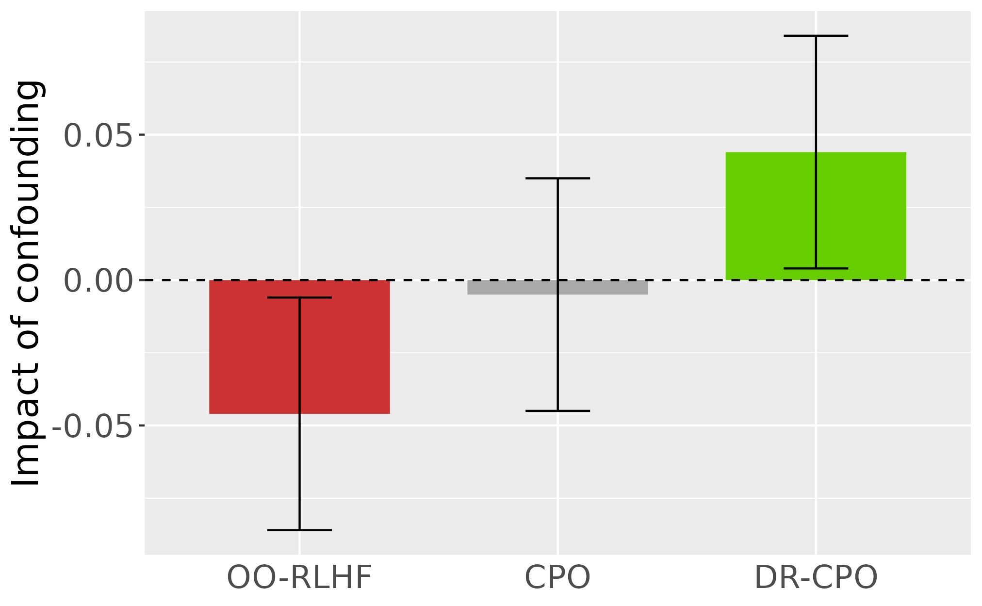
Figure 2: Impact of confounding (measured in win rate difference divided by 2) on OO-RLHF, CPO, and DR-CPO. A negative impact indicates that confounding hurts the performance of the method. Win rates are computed across 600 pairs for each method combination.

6.2 Text Preferences

We report CPO and DR-CPO win rates against OO-RLHF and FT (and against one another) in Figure 1. In Figure 2, we examine the impact of confounding on OO-RLHF, CPO, and DR-CPO. Additional results are found in Appendix C.2.

Outcome optimization (Figure 1). On the Hate Speech dataset, we observe that DR-CPO outperforms both the OO-RLHF and FT baselines. Against both baselines, DR-CPO’s win rate is statistically significant at the 95% confidence level, with the lower bound of its 95% confidence intervals falling above 0.5. These results indicate that using DR-CPO, language models successfully learn human preferences for less hateful text from direct outcomes.

DR-CPO further appears to outperform CPO on the Hate Speech dataset, though its win rate is just shy of statistical significance. These results demonstrate the empirical benefits of double robustness, wherein a good $\widehat{P}^{R}$ provides bias-correction against a poorer $\widehat{g}$ (the former evidenced by DR-CPO’s relatively smaller win rate margin against CPO, and the latter evidenced by DR-CPO’s larger win rate margin against OO-RLHF).

On the Hong Kong dataset, we likewise observe that CPO outperforms both the OO-RLHF and FT baselines. In this setting, CPO achieves statistically significant win rates against both baselines, with the lower bound of its 95% confidence intervals falling above 0.5.

Here, in contrast to the Hate Speech dataset, CPO also outperforms DR-CPO, which suggests that CPO can be very strong under conditions where $P^{R}$ is well controlled or can be estimated very well—as is the case for the Hong Kong dataset, where texts are not only randomly assigned to annotators but programmatically generated from random attributes. Furthermore, we note that outcome models trained on the Hong Kong dataset do not achieve good performance or generalization outside of the training data, possibly due to the artificial nature and relative homogeneity of the texts. Therefore, our results point to a conclusion that under conditions where the outcome model is particularly difficult to learn, CPO may enjoy empirical advantages over DR-CPO despite the theoretical robustness of the latter.

Double robustness under confounding (Figure 2). Finally, on the Confounded dataset, we find that DR-CPO remains robust under confounding, while OO-RLHF degrades significantly. (Vanilla CPO is not affected by confounding because it does not use an outcome model, but we train two separate models to account for randomness in the optimization process.) OO-RLHF experiences a negative impact to win rate that is significantly lower than 0, while CPO experiences no impact and DR-CPO experiences a positive impact. Exploring this last result is an avenue for future work.

These results further illustrate the doubly robust properties of DR-CPO and the shortcomings of outcome modeling approaches. Even under aggressive confounding, with a worst-case outcome model that has been trained on completely negated data, DR-CPO is not compromised, while OO-RLHF is.

We reiterate that because they are optimized on randomized experimental data, $\mathcal{D}_{R}$, CPO and DR-CPO are causal approaches. Taken together, our results constitute empirical evidence for a core theoretical strength—robustness to confounding—of an optimization framework that maintains the causal relationship between text and outcome.

7 Conclusion

In this paper, we explore language model optimization for human preferences from direct outcome datasets, in which each sample consists of a text and the reader’s numerical response. We first posit that language model optimization should be viewed as a causal problem to ensure that the model correctly learns the relationship between the text and the outcome, and we define conditions under which this causal relationship can be guaranteed. Following this, we introduce CPO, a method that solves an unbiased surrogate objective for the causal language optimization problem—and improve upon it with the doubly robust DR-CPO, which reduces the variance of the CPO objective while retaining provably strong guarantees on bias. Finally, we empirically demonstrate the effectiveness of (DR-)CPO in optimizing state-of-the-art LLMs for human preferences on direct outcome data, and we validate the robustness of DR-CPO under difficult confounding conditions. These theoretical contributions and results open the door to a wide range of data, human preferences, and optimization goals that language models can learn using CPO.

Several natural lines of future research follow from this work. For instance, (DR-)CPO may benefit empirically from exploration of entropy regularization techniques that are common in policy optimization. Additionally, future work may wish to extend DR-CPO to the paired completion data setting, as the bias guarantees and variance reduction of a doubly robust approach can also be useful for paired data.

Optimizing Language Models for Human Preferences
 is a Causal Inference Problem
(Supplementary Material)

Appendix A Technical results

A.1 Identifying $V(f)$

Proof.

Proof of Proposition 4.1

We can show that $V(f)=\mathbb{E}_{Y(\cdot)\sim\mathcal{G}}[\mathbb{E}_{X\sim P^{f}}[Y(X)]]=\mathbb{E}_{Y\sim P^{R}_{y}}[\mathbb{E}_{X\sim P^{R}}[\frac{P^{f}(X)}{P^{R}(X)}Y]]$.

$$V(f) =\mathbb{E}_{Y(\cdot)\sim\mathcal{G}}[\mathbb{E}_{X\sim P^{f}}[Y(X)]]$$

$$=\mathbb{E}_{Y(\cdot)\sim\mathcal{G}}\Bigg{[}\sum_{x\in\mathcal{X}}P^{f}(x)Y(x)\Bigg{]}$$

$$=\mathbb{E}_{Y(\cdot)\sim\mathcal{G}}\Bigg{[}\sum_{x\in\mathcal{X}}P^{R}(x)\frac{P^{f}(x)}{P^{R}(x)}Y(x)\Bigg{]}$$

$$=\mathbb{E}_{Y(\cdot)\sim\mathcal{G}}\Bigg{[}\mathbb{E}_{X\sim P^{R}}\Bigg{[}\frac{P^{f}(X)}{P^{R}(X)}Y(X)\Bigg{]}\Bigg{]}$$

$$=\mathbb{E}_{Y\sim P^{R}_{y}}\Bigg{[}\mathbb{E}_{X\sim P^{R}}\Bigg{[}\frac{P^{f}(X)}{P^{R}(X)}Y\Bigg{]}\Bigg{]}$$

∎

Proof.

Proof of Proposition 4.3

We can show that $V(f)=\mathbb{E}_{Y(\cdot)\sim\mathcal{G}}[\mathbb{E}_{X\sim P^{f}}[Y(X)]]=\mathbb{E}_{Y\sim P^{R}_{y}}[\mathbb{E}_{X\sim P^{R}}[\frac{P^{f}(X)}{P^{R}(X)}(Y-g(X))]]+\mathbb{E}_{X\sim P^{f}}[g(X)]$.

$$V(f) =\mathbb{E}_{Y\sim P^{R}_{y}}\Bigg{[}\mathbb{E}_{X\sim P^{R}}\Bigg{[}\frac{P^{f}(X)}{P^{R}(X)}Y\Bigg{]}\Bigg{]}$$ (Proposition 4.1)

$$=\mathbb{E}_{Y\sim P^{R}_{y}}\Bigg{[}\mathbb{E}_{X\sim P^{R}}\Bigg{[}\frac{P^{f}(X)}{P^{R}(X)}(Y-g(X)+g(X))\Bigg{]}\Bigg{]}$$

$$=\mathbb{E}_{Y\sim P^{R}_{y}}\Bigg{[}\mathbb{E}_{X\sim P^{R}}\Bigg{[}\frac{P^{f}(X)}{P^{R}(X)}(Y-g(X))\Bigg{]}\Bigg{]}+\mathbb{E}_{Y\sim P^{R}_{y}}\Bigg{[}\mathbb{E}_{X\sim P^{R}}\Bigg{[}\frac{P^{f}(X)}{P^{R}(X)}g(X)\Bigg{]}\Bigg{]}$$

$$=\mathbb{E}_{Y\sim P^{R}_{y}}\Bigg{[}\mathbb{E}_{X\sim P^{R}}\Bigg{[}\frac{P^{f}(X)}{P^{R}(X)}(Y-g(X))\Bigg{]}\Bigg{]}+\mathbb{E}_{X\sim P^{R}}\Bigg{[}\frac{P^{f}(X)}{P^{R}(X)}g(X)\Bigg{]}$$

$$=\mathbb{E}_{Y\sim P^{R}_{y}}\Bigg{[}\mathbb{E}_{X\sim P^{R}}\Bigg{[}\frac{P^{f}(X)}{P^{R}(X)}(Y-g(X))\Bigg{]}\Bigg{]}+\sum_{x\in\mathcal{X}}P^{R}(x)\frac{P^{f}(x)}{P^{R}(x)}g(x)$$

$$=\mathbb{E}_{Y\sim P^{R}_{y}}\Bigg{[}\mathbb{E}_{X\sim P^{R}}\Bigg{[}\frac{P^{f}(X)}{P^{R}(X)}(Y-g(X))\Bigg{]}\Bigg{]}+\sum_{x\in\mathcal{X}}P^{f}(x)g(x)$$

$$=\mathbb{E}_{Y\sim P^{R}_{y}}\Bigg{[}\mathbb{E}_{X\sim P^{R}}\Bigg{[}\frac{P^{f}(X)}{P^{R}(X)}(Y-g(X))\Bigg{]}\Bigg{]}+\mathbb{E}_{X\sim P^{f}}[g(X)]$$

∎

A.2 Unbiasedness proofs and variance difference

Proof.

Proof of Theorem 4.2

We can show that $\mathbb{E}_{Y(\cdot)\sim\mathcal{G}}[\mathbb{E}_{X}[\widehat{V}_{IPW}(f)]]=\mathbb{E}_{Y(\cdot)\sim\mathcal{G}}[\mathbb{E}_{X\sim P^{f}}[Y(X)]]=V(f)$ when $P^{R}$ is known.

$$\mathbb{E}_{Y(\cdot)\sim\mathcal{G}}[\mathbb{E}_{X\sim P^{R}}[\widehat{V}_{IPW}(f)]] =\mathbb{E}_{Y(\cdot)\sim\mathcal{G}}\Bigg{[}\mathbb{E}_{X\sim P^{R}}\Bigg{[}\frac{1}{n}\sum_{i=1}^{n}\frac{P^{f}(X_{i})}{P^{R}(X_{i})}Y_{i}\Bigg{]}\Bigg{]}$$

$$=\frac{1}{n}\sum_{i=1}^{n}\mathbb{E}_{Y(\cdot)\sim\mathcal{G}}\Bigg{[}\mathbb{E}_{X\sim P^{R}}\Bigg{[}\frac{P^{f}(X_{i})}{P^{R}(X_{i})}Y_{i}\Bigg{]}\Bigg{]}$$

$$=\mathbb{E}_{Y(\cdot)\sim\mathcal{G}}\Bigg{[}\mathbb{E}_{X\sim P^{R}}\Bigg{[}\sum_{x\in\mathcal{X}}\frac{P^{f}(x)}{P^{R}(x)}Y(x)\mathbbm{1}\{X=x\}\Bigg{]}\Bigg{]}$$

$$=\mathbb{E}_{Y(\cdot)\sim\mathcal{G}}\Bigg{[}\sum_{x\in\mathcal{X}}\frac{P^{f}(x)}{P^{R}(x)}Y(x)\underbrace{\mathbb{E}_{X\sim P^{R}}[\mathbbm{1}\{X=x\}]}_{P^{R}(x)}\Bigg{]}$$

$$=\mathbb{E}_{Y(\cdot)\sim\mathcal{G}}\Bigg{[}\sum_{x\in\mathcal{X}}P^{f}(x)Y(x)\Bigg{]}$$

$$=\mathbb{E}_{Y(\cdot)\sim\mathcal{G}}[\mathbb{E}_{X\sim P^{f}}[Y(X)]]$$

$$=V(f)$$

∎

Proof.

Proof of Theorem 4.4

We can show that $\mathbb{E}_{Y(\cdot)\sim\mathcal{G}}[\mathbb{E}_{X}[\widehat{V}_{DR}(f)]]=\mathbb{E}_{Y(\cdot)\sim\mathcal{G}}[\mathbb{E}_{X\sim P^{f}}[Y(X)]]=V(f)$ under one of two conditions: $\widehat{P}^{R}(X)=P^{R}(X)$ (i.e., $P^{R}$ is known) or (2) $\widehat{g}(X)=g(X)=E_{Y(\cdot)\sim\mathcal{G}}[Y(X)]$ (i.e., $g(X)$ is known).

First, we rewrite $\mathbb{E}_{Y(\cdot)\sim\mathcal{G}}[\mathbb{E}_{X}[\widehat{V}_{DR}(f)]]$:

$$\mathbb{E}_{Y(\cdot)\sim\mathcal{G}}[\mathbb{E}_{X,\widetilde{X}}[\widehat{V}_{DR}(f)]]= \;\mathbb{E}_{Y(\cdot)\sim\mathcal{G}}\Bigg{[}\mathbb{E}_{X,\widetilde{X}}\Bigg{[}\frac{1}{n}\sum_{i=1}^{n}\frac{P^{f}(X_{i})}{\widehat{P}^{R}(X_{i})}(Y_{i}-\widehat{g}(X_{i}))+\frac{1}{m}\sum_{j=1}^{m}\frac{P^{f}(\widetilde{X}_{j})}{P^{f^{0}}(\widetilde{X}_{j})}\widehat{g}(\widetilde{X}_{j})\Bigg{]}\Bigg{]}$$

$$= \;\mathbb{E}_{Y(\cdot)\sim\mathcal{G}}\Bigg{[}\mathbb{E}_{X\sim P^{R}}\Bigg{[}\frac{1}{n}\sum_{i=1}^{n}\frac{P^{f}(X_{i})}{\widehat{P}^{R}(X_{i})}(Y_{i}-\widehat{g}(X_{i}))\Bigg{]}\Bigg{]}$$

$$+\mathbb{E}_{Y(\cdot)\sim\mathcal{G}}\Bigg{[}\mathbb{E}_{\widetilde{X}\sim P^{f^{0}}}\Bigg{[}\frac{1}{m}\sum_{j=1}^{m}\frac{P^{f}(\widetilde{X}_{j})}{P^{f^{0}}(\widetilde{X}_{j})}\widehat{g}(\widetilde{X}_{j})\Bigg{]}\Bigg{]}$$

$$= \;\frac{1}{n}\sum_{i=1}^{n}\mathbb{E}_{Y(\cdot)\sim\mathcal{G}}\Bigg{[}\mathbb{E}_{X\sim P^{R}}\Bigg{[}\frac{P^{f}(X_{i})}{\widehat{P}^{R}(X_{i})}(Y_{i}-\widehat{g}(X_{i}))\Bigg{]}\Bigg{]}$$

$$+\frac{1}{m}\sum_{j=1}^{m}\mathbb{E}_{Y(\cdot)\sim\mathcal{G}}\Bigg{[}\mathbb{E}_{\widetilde{X}\sim P^{f^{0}}}\Bigg{[}\frac{P^{f}(\widetilde{X}_{j})}{P^{f^{0}}(\widetilde{X}_{j})}\widehat{g}(\widetilde{X}_{j})\Bigg{]}\Bigg{]}$$

Case (1) $\widehat{P}^{R}(X)=P^{R}(X)$:

Rewriting the first term,

$$\frac{1}{n}\sum_{i=1}^{n}\mathbb{E}_{Y(\cdot)\sim\mathcal{G}}\Bigg{[}\mathbb{E}_{X\sim P^{R}}\Bigg{[}\frac{P^{f}(X_{i})}{\widehat{P}^{R}(X_{i})}(Y_{i}-\widehat{g}(X_{i}))\Bigg{]}\Bigg{]} =\frac{1}{n}\sum_{i=1}^{n}\mathbb{E}_{Y(\cdot)\sim\mathcal{G}}\Bigg{[}\mathbb{E}_{X\sim P^{R}}\Bigg{[}\frac{P^{f}(X_{i})}{P^{R}(X_{i})}(Y_{i}-\widehat{g}(X_{i}))\Bigg{]}\Bigg{]}$$

$$=\mathbb{E}_{Y(\cdot)\sim\mathcal{G}}\Bigg{[}\mathbb{E}_{X\sim P^{R}}\Bigg{[}\sum_{x\in\mathcal{X}}\frac{P^{f}(x)}{P^{R}(x)}(Y(x)-\widehat{g}(x))\mathbbm{1}\{X=x\}\Bigg{]}\Bigg{]}$$

$$=\mathbb{E}_{Y(\cdot)\sim\mathcal{G}}\Bigg{[}\sum_{x\in\mathcal{X}}\frac{P^{f}(x)}{P^{R}(x)}(Y(x)-\widehat{g}(x))\underbrace{\mathbb{E}_{X\sim P^{R}}[\mathbbm{1}\{X=x\}]}_{P^{R}(x)}\Bigg{]}$$

$$=\mathbb{E}_{Y(\cdot)\sim\mathcal{G}}\Bigg{[}\sum_{x\in\mathcal{X}}P^{f}(x)(Y(x)-\widehat{g}(x))\Bigg{]}$$

$$=\mathbb{E}_{Y(\cdot)\sim\mathcal{G}}[\mathbb{E}_{X\sim P^{f}}[Y(X)-\widehat{g}(X)]]$$

$$=\mathbb{E}_{Y(\cdot)\sim\mathcal{G}}[\mathbb{E}_{X\sim P^{f}}[Y(X)]]-\mathbb{E}_{Y(\cdot)\sim\mathcal{G}}[\mathbb{E}_{X\sim P^{f}}[\widehat{g}(X)]]$$

Rewriting the second term,

$$\frac{1}{m}\sum_{j=1}^{m}\mathbb{E}_{Y(\cdot)\sim\mathcal{G}}\Bigg{[}\mathbb{E}_{\widetilde{X}\sim P^{f^{0}}}\Bigg{[}\frac{P^{f}(\widetilde{X}_{j})}{P^{f^{0}}(\widetilde{X}_{j})}\widehat{g}(\widetilde{X}_{j})\Bigg{]}\Bigg{]} =\mathbb{E}_{Y(\cdot)\sim\mathcal{G}}\Bigg{[}\mathbb{E}_{\widetilde{X}\sim P^{f^{0}}}\Bigg{[}\sum_{x\in\mathcal{X}}\frac{P^{f}(x)}{P^{f^{0}}(x)}\widehat{g}(x)\mathbbm{1}\{\widetilde{X}=x\}\Bigg{]}\Bigg{]}$$

$$=\mathbb{E}_{Y(\cdot)\sim\mathcal{G}}\Bigg{[}\sum_{x\in\mathcal{X}}\frac{P^{f}(x)}{P^{f^{0}}(x)}\widehat{g}(x)\underbrace{\mathbb{E}_{\widetilde{X}\sim P^{f^{0}}}[\mathbbm{1}\{\widetilde{X}=x\}]}_{P^{f^{0}}(x)}\Bigg{]}$$

$$=\mathbb{E}_{Y(\cdot)\sim\mathcal{G}}\Bigg{[}\sum_{x\in\mathcal{X}}P^{f}(x)\widehat{g}(x)\Bigg{]}$$

$$=\mathbb{E}_{Y(\cdot)\sim\mathcal{G}}[\mathbb{E}_{X\sim P^{f}}[\widehat{g}(X)]]$$

Then we have

$$\mathbb{E}_{Y(\cdot)\sim\mathcal{G}}[\mathbb{E}_{X}[\widehat{V}_{DR}(f)]] =\mathbb{E}_{Y(\cdot)\sim\mathcal{G}}[\mathbb{E}_{X\sim P^{f}}[Y(X)]]-\mathbb{E}_{Y(\cdot)\sim\mathcal{G}}[\mathbb{E}_{X\sim P^{f}}[\widehat{g}(X)]]+\mathbb{E}_{Y(\cdot)\sim\mathcal{G}}[\mathbb{E}_{X\sim P^{f}}[\widehat{g}(X)]]$$

$$=\mathbb{E}_{Y(\cdot)\sim\mathcal{G}}[\mathbb{E}_{X\sim P^{f}}[Y(X)]]$$

$$=V(f)$$

Case (2) $\widehat{g}(X)=g(X)=E_{Y(\cdot)\sim\mathcal{G}}[Y(X)]$:

Rewriting the first term,

$$\frac{1}{n}\sum_{i=1}^{n}\mathbb{E}_{Y(\cdot)\sim\mathcal{G}}\Bigg{[}\mathbb{E}_{X\sim P^{R}}\Bigg{[}\frac{P^{f}(X_{i})}{\widehat{P}^{R}(X_{i})}(Y_{i}-\widehat{g}(X_{i}))\Bigg{]}\Bigg{]} =\frac{1}{n}\sum_{i=1}^{n}\mathbb{E}_{Y(\cdot)\sim\mathcal{G}}\Bigg{[}\mathbb{E}_{X\sim P^{R}}\Bigg{[}\frac{P^{f}(X_{i})}{\widehat{P}^{R}(X_{i})}(Y_{i}-g(X_{i}))\Bigg{]}\Bigg{]}$$

$$=\mathbb{E}_{Y(\cdot)\sim\mathcal{G}}\Bigg{[}\mathbb{E}_{X\sim P^{R}}\Bigg{[}\sum_{x\in\mathcal{X}}\frac{P^{f}(x)}{\widehat{P}^{R}(x)}(Y(x)-g(x))\mathbbm{1}\{X=x\}\Bigg{]}\Bigg{]}$$

$$=\mathbb{E}_{Y(\cdot)\sim\mathcal{G}}\Bigg{[}\sum_{x\in\mathcal{X}}\frac{P^{f}(x)}{\widehat{P}^{R}(x)}(Y(x)-g(x))\underbrace{\mathbb{E}_{X\sim P^{R}}[\mathbbm{1}\{X=x\}]}_{P^{R}(x)}\Bigg{]}$$

$$=\mathbb{E}_{Y(\cdot)\sim\mathcal{G}}\Bigg{[}\sum_{x\in\mathcal{X}}\frac{P^{f}(x)P^{R}(x)}{\widehat{P}^{R}(x)}(Y(x)-g(x))\Bigg{]}$$

$$=\sum_{x\in\mathcal{X}}\frac{P^{f}(x)P^{R}(x)}{\widehat{P}^{R}(x)}\mathbb{E}_{Y(\cdot)\sim\mathcal{G}}[Y(x)-g(x)]$$

$$=\sum_{x\in\mathcal{X}}\frac{P^{f}(x)P^{R}(x)}{\widehat{P}^{R}(x)}(\mathbb{E}_{Y(\cdot)\sim\mathcal{G}}[Y(x)]-g(x))$$

$$=\sum_{x\in\mathcal{X}}\frac{P^{f}(x)P^{R}(x)}{\widehat{P}^{R}(x)}\cdot 0$$

$$=0$$

Rewriting the second term,

$$\frac{1}{m}\sum_{j=1}^{m}\mathbb{E}_{Y(\cdot)\sim\mathcal{G}}\Bigg{[}\mathbb{E}_{\widetilde{X}\sim P^{f^{0}}}\Bigg{[}\frac{P^{f}(\widetilde{X}_{j})}{P^{f^{0}}(\widetilde{X}_{j})}\widehat{g}(\widetilde{X}_{j})\Bigg{]}\Bigg{]} =\frac{1}{m}\sum_{j=1}^{m}\mathbb{E}_{Y(\cdot)\sim\mathcal{G}}\Bigg{[}\mathbb{E}_{\widetilde{X}\sim P^{f^{0}}}\Bigg{[}\frac{P^{f}(\widetilde{X}_{j})}{P^{f^{0}}(\widetilde{X}_{j})}g(\widetilde{X}_{j})\Bigg{]}\Bigg{]}$$

$$=\mathbb{E}_{Y(\cdot)\sim\mathcal{G}}\Bigg{[}\mathbb{E}_{\widetilde{X}\sim P^{f^{0}}}\Bigg{[}\sum_{x\in\mathcal{X}}\frac{P^{f}(x)}{P^{f^{0}}(x)}g(x)\mathbbm{1}\{\widetilde{X}=x\}\Bigg{]}\Bigg{]}$$

$$=\mathbb{E}_{Y(\cdot)\sim\mathcal{G}}\Bigg{[}\sum_{x\in\mathcal{X}}\frac{P^{f}(x)}{P^{f^{0}}(x)}g(x)\underbrace{\mathbb{E}_{\widetilde{X}\sim P^{f^{0}}}[\mathbbm{1}\{\widetilde{X}=x\}]}_{P^{f^{0}}(x)}\Bigg{]}$$

$$=\mathbb{E}_{Y(\cdot)\sim\mathcal{G}}\Bigg{[}\sum_{x\in\mathcal{X}}P^{f}(x)g(x)\Bigg{]}$$

$$=\sum_{x\in\mathcal{X}}P^{f}(x)g(x)$$

$$=\mathbb{E}_{X\sim P^{f}}[g(X)]$$

$$=\mathbb{E}_{X\sim P^{f}}[E_{Y(\cdot)\sim\mathcal{G}}[Y(X)]]$$

$$=\mathbb{E}_{Y(\cdot)\sim\mathcal{G}}[\mathbb{E}_{X\sim P^{f}}[Y(X)]]$$

Then we have

$$\mathbb{E}_{Y(\cdot)\sim\mathcal{G}}[\mathbb{E}_{X}[\widehat{V}_{DR}(f)]] =0+\mathbb{E}_{Y(\cdot)\sim\mathcal{G}}[\mathbb{E}_{X\sim P^{f}}[Y(X)]]$$

$$=\mathbb{E}_{Y(\cdot)\sim\mathcal{G}}[\mathbb{E}_{X\sim P^{f}}[Y(X)]]$$

$$=V(f)$$

∎

Proof.

Proof of Proposition 4.5

First, we compute the variance of $\widehat{V}_{IPW}(f)$, where $X_{i}\sim P^{R}$ and $Y_{i}\sim P^{R}_{y}$ i.i.d.

$$\text{Var}\left(\widehat{V}_{IPW}(f)\right) =\text{Var}\left(\frac{1}{n}\sum_{i=1}^{n}\frac{P^{f}(X_{i})}{P^{R}(X_{i})}Y_{i}\right)$$

$$=\frac{1}{n^{2}}\sum_{i=1}^{n}\text{Var}\left(\frac{P^{f}(X_{i})}{P^{R}(X_{i})}Y_{i}\right)$$

$$=\frac{1}{n}\text{Var}\left(\frac{P^{f}(X)}{P^{R}(X)}Y\right)$$

$$=\frac{1}{n}\mathbb{E}\left[\text{Var}\left(\frac{P^{f}(X)}{P^{R}(X)}Y\mid X\right)\right]+\frac{1}{n}\text{Var}\left(\mathbb{E}\left[\frac{P^{f}(X)}{P^{R}(X)}Y\mid X\right]\right)$$

$$=\frac{1}{n}\mathbb{E}\left[\frac{P^{f}(X)^{2}}{P^{R}(X)^{2}}\text{Var}\left(Y\mid X\right)\right]+\frac{1}{n}\text{Var}\left(\frac{P^{f}(X)}{P^{R}(X)}\mathbb{E}\left[Y\mid X\right]\right)$$

$$=\frac{1}{n}\mathbb{E}\left[\frac{P^{f}(X)^{2}}{P^{R}(X)^{2}}\text{Var}\left(Y\mid X\right)\right]+\frac{1}{n}\text{Var}\left(\frac{P^{f}(X)}{P^{R}(X)}g(X)\right)$$

where we have used that under randomization $\mathbb{E}[Y\mid X=x]=\mathbb{E}_{Y(\cdot)\sim\mathcal{G}}[Y(x)]=g(x)$.

For the variance of $\widehat{V}_{DR}(f)$, we first note that if $\widehat{g}$ is fit on a separate, independent sample, we have that

$$\text{Var}\left(\widehat{V}_{DR}(f)\right) =\text{Var}\left(\frac{1}{n}\sum_{i=1}^{n}\frac{P^{f}(X_{i})}{P^{R}(X_{i})}(Y_{i}-\widehat{g}(X_{i}))+\frac{1}{m}\sum_{j=1}^{m}\frac{P^{f}(\widetilde{X}_{j})}{P^{f^{0}}(\widetilde{X}_{j})}\widehat{g}(\widetilde{X}_{j})\right)$$

$$=\frac{1}{n^{2}}\sum_{i=1}^{n}\text{Var}\left(\frac{P^{f}(X_{i})}{P^{R}(X_{i})}(Y_{i}-\widehat{g}(X_{i}))\right)+\frac{1}{m^{2}}\sum_{j=1}^{m}\text{Var}\left(\frac{P^{f}(\widetilde{X}_{j})}{P^{f^{0}}(\widetilde{X}_{j})}\widehat{g}(\widetilde{X}_{j})\right)$$

$$=\frac{1}{n}\underbrace{\text{Var}\left(\frac{P^{f}(X)}{P^{R}(X)}(Y-\widehat{g}(X))\right)}_{(\ast)}+\frac{1}{m}\text{Var}\left(\frac{P^{f}(\widetilde{X})}{P^{f^{0}}(\widetilde{X})}\widehat{g}(\widetilde{X})\right)$$

where $X\sim P^{R}$, $Y\sim P^{R}_{y}$, and $\widetilde{X}\sim P^{f^{0}}$. Now notice that

$$(\ast) =\mathbb{E}\left[\text{Var}\left(\frac{P^{f}(X)}{P^{R}(X)}(Y-\widehat{g}(X))\mid X\right)\right]+\text{Var}\left(\mathbb{E}\left[\frac{P^{f}(X)}{P^{R}(X)}(Y-\widehat{g}(X))\mid X\right]\right)$$

$$=\mathbb{E}\left[\frac{P^{f}(X)^{2}}{P^{R}(X)^{2}}\text{Var}\left(Y\mid X\right)\right]+\text{Var}\left(\frac{P^{f}(X)}{P^{R}(X)}\left(g(X)-\widehat{g}(X)\right)\right)$$

∎

A.3 Equivalence of $V_{out}(f)$

We can show that our rewriting of $V_{out}(f)$ is equivalent to our original definition:

$$V_{out}(f) =\mathbb{E}_{\widetilde{X}\sim P^{f^{0}}}\Bigg{[}\frac{P^{f}(X)}{P^{f^{0}}(X)}g(X)\Bigg{]}$$

$$=\sum_{x\in\mathcal{X}}P^{f^{0}}(x)\frac{P^{f}(x)}{P^{f^{0}}(x)}g(x)$$

$$=\sum_{x\in\mathcal{X}}P^{f}(x)g(x)$$

$$=E_{X\sim P^{f}}[g(X)]$$

Appendix B Parallels between RLHF and optimization of $V_{out}(f)$

The loss function under RLHF is typically computed through proximal policy optimization (PPO):

$$\mathcal{L}(\theta,\phi)=\mathcal{L}^{PPO}_{\text{policy}}(\theta)+c_{1}\mathcal{L}^{PPO}_{\text{value}}(\phi)-c_{2}\mathcal{L}^{PPO}_{\text{entropy}}(\theta)$$

where $\mathcal{L}^{PPO}_{\text{value}}(\phi)$ and $\mathcal{L}^{PPO}_{\text{entropy}}(\theta)$ are regularization terms and $\mathcal{L}^{PPO}_{\text{policy}}(\theta)$ is the policy loss. Letting $p$ denote the prompt, $c$ denote the completion, and $r$ denote the reward model, we consider only the policy loss without any stability tricks like clipping. $\pi_{\theta}$ is the probability under the policy being optimized, while $\pi_{\theta_{0}}$ is the probability under a reference policy (often the starting policy or the policy at the previous step).

$$\mathcal{L}_{PPO}(\theta)=\mathbb{E}\left[\frac{\pi_{\theta}(c|p)}{\pi_{\theta_{0}}(c|p)}\cdot r(p,c)\right]$$

We can see the equivalence between $\pi_{\theta}(c|p)$ and $P^{f}(X)$, $\pi_{\theta_{0}}(c|p)$ and $P^{f^{0}}(X)$, and $r(p,c)$ and $g(X)$; substituting these terms renders $\mathcal{L}_{PPO}$ equal to $V_{out}(f)$.

Appendix C Experiments

C.1 GPT-4 Win Rate Prompts

In this section, we include the inputs provided to GPT-4 for each dataset to obtain its preferences between texts generated by different methods. We use gpt-4-1106-preview from the OpenAI API. We adapt the prompt formats described in Rafailov et al. [2023]. The order of texts is random for each evaluation. For a (method, baseline) comparison, method corresponds to text A 50% of the time and text B 50% of the time.

C.1.1 Hate Speech prompt

⬇

Hate speech is a direct attack on an individual based on protected characteristics: race, ethnicity, national origin, religious affiliation, sexual orientation, caste, sex, gender, gender identity, and serious disease or disability.

Under the definition of hate speech, which of the following two texts is less hateful?

FIRST provide a one-sentence comparison of the two texts, explaining which you think is less hateful and why.

SECOND, on a new line, state only "A" or "B" to indicate your choice. Your response should use the format:

Comparison: <one-sentence comparison and explanation>

Preferred: <"A" or "B">

A: <text A>

B: <text B>

C.1.2 Hong Kong and Confounded prompt

⬇

In March 2019, the Hong Kong government proposed a bill that would have allowed certain criminal suspects to be extradited to mainland China for trial. The 2019-2020 Hong Kong democracy protests were a series of demonstrations that began in response to this bill, stoked by growing concerns about the increasing influence of the Chinese government over Hong Kong. Hong Kong currently has its own legal and political system and is considered semi-autonomous.

Which of the following two texts better convinces you that the U.S. government should support the Hong Kong democracy protesters?

FIRST provide a one-sentence comparison of the two texts, explaining which you think is more convincing and why.

SECOND, on a new line, state only "A" or "B" to indicate your choice. Your response should use the format:

Comparison: <one-sentence comparison and explanation>

Preferred: <"A" or "B">

A: <text A>

B: <text B>

C.2 Additional Results

	Hong Kong		Hate Speech
	CPO win rate	DR-CPO win rate	CPO win rate	DR-CPO win rate
FT	0.528* [0.506, 0.550]	0.477 [0.455, 0.499]	0.517 [0.495, 0.539]	0.524* [0.502, 0.546]
CPO	-	0.441 [0.419, 0.463]	-	0.518 [0.496, 0.540]
OO-RLHF	0.542* [0.520, 0.564]	0.482 [0.460, 0.504]	0.538* [0.516, 0.560]	0.560* [0.538, 0.582]
DR-CPO	0.559* [0.537, 0.581]	-	0.482 [0.460, 0.504]	-

Table 2: CPO and DR-CPO win rates against OO-RLHF, FT, and each other. A win rate exceeding 0.5 indicates that the named method outperforms the competing method with respect to the target outcome. Win rates are computed across 2000 pairs for each method combination.

	Unconfounded win rate over confounded
OO-RLHF	0.546* [0.506, 0.586]
DR-CPO	0.456* [0.416, 0.496]
CPO	0.505 [0.465, 0.545]

Table 3: Win rates with outcome models trained on unconfounded data (Hong Kong) vs. confounded data (Confounded). A win rate exceeding 0.5 indicates that the method+unconfounded outcome model outperforms the method+confounded outcome model with respect to the target outcome—in other words, that confounding hurts the method. Win rates are computed across 600 pairs for each method combination.

We include the full set of CPO and DR-CPO win rates against OO-RLHF and FT and against each other (Table 2). We also include raw win rates from the confounding experiments, specifically win rates of unconfounded methods over confounded methods (Table 3). We briefly discuss comparisons that did not appear in the main body of the paper.

On the Hate Speech dataset, we observe that CPO—like DR-CPO—also outperforms both the OO-RLHF and FT baselines. Against OO-RLHF, CPO’s win rate is statistically significant at the 95% confidence level, while its win rate against FT falls slightly short of statistical significance.

On the Hong Kong dataset, we find that DR-CPO performs comparably to OO-RLHF but falls short against the other methods. We attribute this to possible difficulty in learning the outcome model itself; this is further evidenced by the strong performance of CPO, which does not use an outcome model. As we mention in the main results, learning a strong outcome model on the Hong Kong dataset may be challenging, as its texts read somewhat artificially due to their programmatic construction.