Unsupervised Domain Adaptation within Deep Foundation Latent Spaces

Abstract

The vision transformer-based foundation models, such as ViT or Dino-V2, are aimed at solving problems with little or no finetuning of features. Using a setting of prototypical networks, we analyse to what extent such foundation models can solve unsupervised domain adaptation without finetuning over the source or target domain. Through quantitative analysis, as well as qualitative interpretations of decision making, we demonstrate that the suggested method can improve upon existing baselines, as well as showcase the limitations of such approach yet to be solved.

1 Introduction

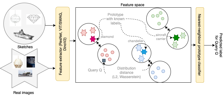
Figure 1: The methodology scheme: (1) the images from multiple domains (e.g., sketches and real images) are embedded into the feature space and, for each domain, separately clustered using $k$-means. The cluster centroids for one of the domains (’source domain’), shown in bright colour in the figure and referred to as ’prototypes’, are provided with labels. (2) Domain adaptation is performed through inter-domain cluster matches with $\ell^{2}$ or Wasserstein distance. (3) Decision making through nearest-neighbour prototype classifier performs the prediction

With the advancement of foundation models, improvements in semi- and unsupervised learning methods can shift from end-to-end training towards decision making over the foundation models’ latent spaces (Oquab et al. (2023); Angelov et al. (2023)).

Below we describe the problem of unsupervised domain adaptation (UDA) (Saenko et al. (2010)). Consider a source image dataset $\mathcal{S}=\{I^{\mathcal{S}}_{1},\ldots I^{\mathcal{S}}_{n}\}$ and a target dataset $\mathcal{T}=\{I^{\mathcal{T}}_{1},\ldots I^{\mathcal{T}}_{m}\}$. These datasets share the same set of classes $\{C_{1}\ldots C_{k}\}$, however the training labels are only known for the source dataset. The problem is, given a classifier trained on a source dataset, to adapt it, without any target data labels, to classify data on a target dataset.

Many of the existing works targeting UDA focus on representation learning approach towards assimilating, in the feature space, the source and target data (Saenko et al. (2010)). For many contemporary works, this is performed using adversarial training or minimising distribution divergence to match the distributions between the source and the target domain (Peng et al. (2019)).

However, such training may not be an option if one wants to avoid finetuning of the latent feature spaces. We address it by using prototypical networks (Snell et al. (2017); Chen et al. (2019); Angelov & Soares (2020)), which recast decision making process into a function of prototypes (Angelov et al. (2023)), derived from the training data. For this purpose, we combine the prototypical network within the latent feature space with distribution matching between source and target domains. In Figure 1, we summarise how one can address UDA problem using a simple combination of clustering and distribution matching within the latent feature spaces using L2 or Wasserstein distances. We show that such approach can lead to promising results on a number of problems and outcompete purpose-finetuned models for UDA; furthermore, it allows to interpret the reasons behind misclassification using geometric proximity analysis through latent feature spaces.

2 Related work

Unsupervised domain adaptation

Saenko et al. (2010) described a problem of adaptation to visual domain shifts, where the model is trained on the source domain and tested on the target one, with changes in lighting, background, viewpoint, amongst others. The current methods to solve this problem use a variety of approaches including adversarial assimilation of source and target distribution Tzeng et al. (2017); Zhao et al. (2018); Liu et al. (2021a); Saito et al. (2018), moment matching Zellinger et al. (2017); Peng et al. (2019). Peng et al. (2019) proposes a dataset for UDA and the problem statement for multi-source domain adaptation, where they evaluate the transfer learning when there are multiple source domains.

Visual Transformers

Building upon the applications of the attention models to the natural language processing (Vaswani et al. (2017)), vision transformers (Dosovitskiy et al. (2021)) allowed not only to improve the performance but also provide generalisation capabilities (Zhang et al. (2022), Oquab et al. (2023)). A substantial amount of literature is devoted to the aspects of pretraining (Singh et al. (2022)), architecture design (Liu et al. (2021b)), unsupervised representation learning (Oquab et al. (2023)), and task-specific finetuning of vision transformers (Dai et al. (2021)).

Transparency of decision making

The pursuit of analysis of existing deep learning models has led to a number of methods targeting aspects of transparency such as ante hoc, by-design, interpretability and post hoc explainability. The former has been manifested by the interpretable-through-prototype methods such as ProtoPNet (Chen et al. (2019)), xDNN (Angelov & Soares (2020)) and IDEAL (Angelov et al. (2023)), as well as explainable architectures such as B-cos (Böhle et al. (2022)). The latter has widely used methods based on the sensitivity analysis for the input data, such as GradCAM (Selvaraju et al. (2017)) and Simonyan et al. (2014). In this work, we focus on prototype-based methods, which allow to interpret the decision-making part through similarity of the query sample to the prototype, and therefore, our work is closely related to prototypical networks.

3 Methodology

Data: Source and target datasets $\mathcal{S},\mathcal{T}$, Source query $q_{s}$, target query $q_{t}$

Result: Source dataset class predictions $\hat{y}^{\mathcal{S}}(q_{s})$, target dataset class predictions $\hat{y}^{\mathcal{T}}(q_{t})$

$\mathcal{S}\leftarrow\phi(\mathcal{S}),\mathcal{T}\leftarrow\phi(\mathcal{T})$ ;

 // $\phi$ denotes feature extractor

$P_{\mathcal{S}}^{c},C_{\mathcal{S}}\leftarrow k$-means $(\mathcal{S},|C_{\mathcal{S}}|)$ ;

 // Clustering of source data, $P_{S}^{c}$ are cluster centroids, $C_{\mathcal{S}}$ are cluster subsets of $\mathcal{S}$

$P_{\mathcal{S}}\leftarrow\{\arg\min_{s\in\mathcal{S}}\ell^{2}(s,p)\forall p\in P_{\mathcal{S}}^{c}\}$;

 // Selecting closest prototypes from $\mathcal{S}$

$P_{\mathcal{T}}^{c},C_{\mathcal{T}}\leftarrow k$-means $(\mathcal{T},|C_{\mathcal{T}}|)$ ;

 // Clustering of target data, $P_{\mathcal{T}}^{c}$ are cluster centroids, $C_{\mathcal{T}}^{c}$ are cluster subsets of $\mathcal{T}$

$P_{\mathcal{T}}\leftarrow\{\arg\min_{t\in\mathcal{T}}\ell^{2}(t,p)\forall p\in P_{\mathcal{T}}^{c}\}$;

 // Selecting closest prototypes from $\mathcal{T}$

$L_{\mathcal{S}}\leftarrow\mathtt{RetrieveLabels}(P_{\mathcal{S}})$ ;

 // Retrieve labels for every source prototype from $P_{\mathcal{S}}$ (and its corresponding cluster)

$D_{\mathcal{ST}}=\mathtt{DistanceMatrix}(C_{\mathcal{S}},P_{\mathcal{S}},C_{\mathcal{T}},P_{\mathcal{T}})$ ;

  // Wasserstein or $l^{2}$ centroid distance matrix between clusters

$L_{T}\leftarrow\mathtt{ClosestMapping}(D_{ST},L_{S})$ ;

  // Target clusters receive labels of the closest source cluster according to the distance matrix $D_{\mathcal{ST}}$

$\hat{y}(q_{s};P_{\mathcal{S}})\leftarrow L_{\mathcal{S}}[\arg\min_{p\in P_{\mathcal{S}}}\ell^{2}(p,q_{s})]$ ;

  // Source query class prediction

$\hat{y}(q_{t};P_{\mathcal{T}})\leftarrow L_{T}[\arg\min_{p\in P_{\mathcal{T}}}\ell^{2}(p,q_{t})]$ ;

  // Target query class prediction

Algorithm 1 Proposed algorithm for UDA

In Algorithm 1, we present the methodology for the proposed analysis. The methodology is split into (1) feature extraction, (2) selection of prototypes through clustering, (3) matching the prototypes between the source and the target domain (4) source and target class prediction.

We use two distinct methods for measuring distance between the clusters: $l^{2}$ distance between cluster prototypes, and the Sinkhorn approximation of the 2-Wasserstein distance (see details of implementation in the Appendix A).

4 Experiments

Experimental conditions

We reproduce the experimental setting from Peng et al. (2019), with the further experimental details described in Appendix A. While in Peng et al. (2019) the model is proposed for the multi-source UDA, we present the results only for a single source domain. The dataset contains six domains: sketch (ske), real (rel), quickdraw (qdr), painting (pnt), infograph (inf), and clipart(clp), each split into the same $345$ categories of common objects.

Table 2(a) shows the performance of the proposed methodology for ResNet-152-based model, as well as for the oracle (purpose-fit model), based on ResNet-152, and for the MCD (Saito et al. (2018)) baseline, based on ResNet-101 (He et al. (2016)), which has shown the best performance in the analysis of Peng et al. (2019). It can be seen that in such scenario the model performs substantially worse than the state-of-the-art UDA method MCD (Saito et al. (2018)). In Tables 2(b)-2(d), we demonstrate that the performance improves for various ViT backbones and ultimately overtakes MCD baseline (Saito et al. (2018)). It happens, however, that superior performance in transfer learning for Dino-V2 (Oquab et al. (2023)) does not translate into a better performance on this UDA task. Furthermore, the version, pretrained on ImageNet-1K (Table 2(c)) surprisingly shows better performance on practically every single task comparing to the counterpart without pretraining (Table 2(b)). Comparison with the Wasserstein distance version of the method demonstrates that while the choice of distance shows some potential to improve the performance, it still lags behind ViT H/14, finetuned on ImageNet-1K.

In Section B, we demonstrate the analysis of the errors in the latent space by visualising the nearest prototypes for SWAG ViT-H/14, finetuned on ImageNet-1K. Such analysis demonstrates remarkable cross-domain generalisation, with a number of justified semantically meaningful errors (for example, mistaking diamonds for similarly-looking blueberries), as well as highlights that some of the errors are caused by preferring texture to the semantics (e.g., mistaking octagon for hexagon).

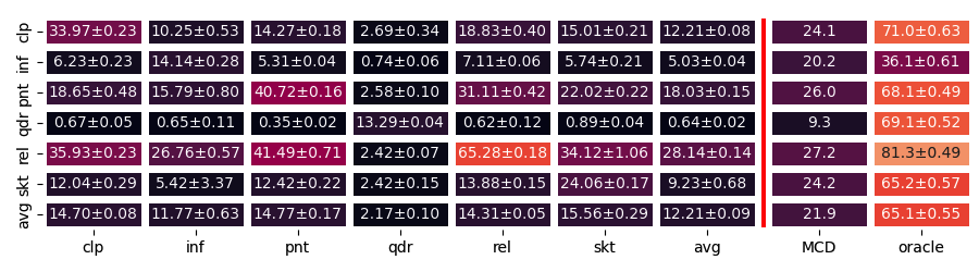
(a) ResNet-152, finetuned on ImageNet, MCD (Saito et al. (2018)) and oracle results are taken from Peng et al. (2019)

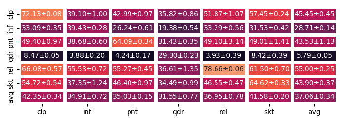
(b) SWAG ViT-H/14 without finetuning ($l^{2}$ cluster prototypes distance)

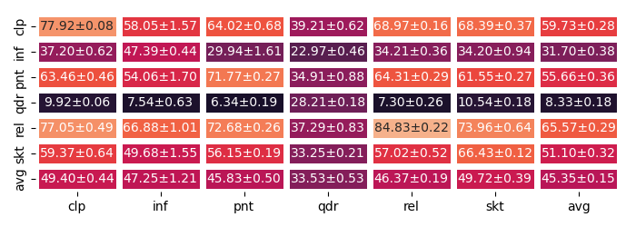
(c) SWAG ViT-H/14, ImageNet1K finetuning ($l^{2}$ cluster prototypes distance)

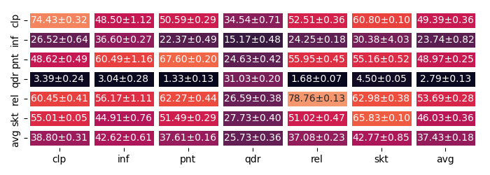
(d) DinoV2 ViT-G/14, no finetuning ($l^{2}$ cluster prototypes distance)

(e) DinoV2 ViT-G/14 (Sinkhorn approximation of the Wasserstein distance)

Figure 2: UDA results for different backbone architectures (columns denote source domains, and rows denote target domains), $k$-means clustering ($5\times 345=1725$ clusters, $345$ classes)

5 Conclusion

We show that, with just fixed ViT feature representation and domain distribution matching, one can solve a number of unsupervised domain adaptation problems within the foundational feature space, exceeding the performance of purpose-built representation learning frameworks for UDA, such as MCD (Saito et al. (2018)) and thus becoming a plausible alternative to finetuning-based domain adaptation. In many cases, however, even though the results are wrong from the benchmark’s point of view, they still can constitute a plausible answer even for the humans (see Figure 3 in the Appendix). The described methodology can serve as a benchmark for evaluating such representation learning. While foundation models provide competitive performance against purpose-built models in this challenge, some of the best-performing models, such as DinoV2 G/14, do not improve upon the performance of older models with lower general-purpose performance, such as SWAG-ViT, finetuned on ImageNet-1K.

Appendix A Experimental setup

We use the pretrained SWAG-ViT (Singh et al. (2022)) models from publicly available repository. SWAG ViT H/14 model corresponds to the pretrained model with no finetuning. For the experiments we use NVIDIA RTX A2000 12GB powered workstation. sklearn implementation of $k$-means clustering is used.

All the experiments are repeated with three different random seeds to calculate the confidence interval, except from the Wasserstein distance experiment in Figure 2(e) which do not include confidence interval computation due to the computational costs.

For calculating the Sinkhorn approximation of 2-Wasserstein distance, we use the following geomloss library function: geomloss.SamplesLoss(loss=’sinkhorn’, p=2, blur=1e-5).

Appendix B Interpretability analysis

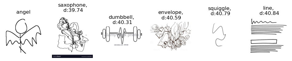
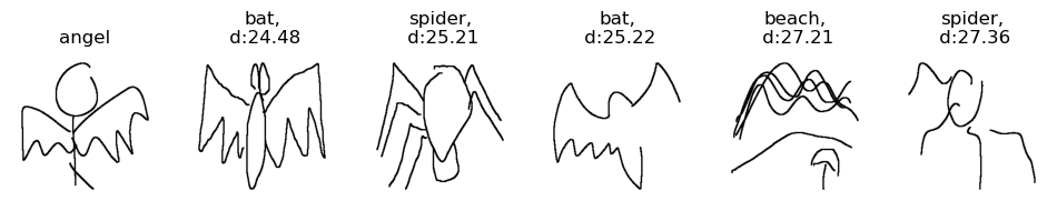
(a) Angel, recognised incorrectly (testing, sketch $\rightarrow$ quickdraw), left: sketch, right: quickdraw

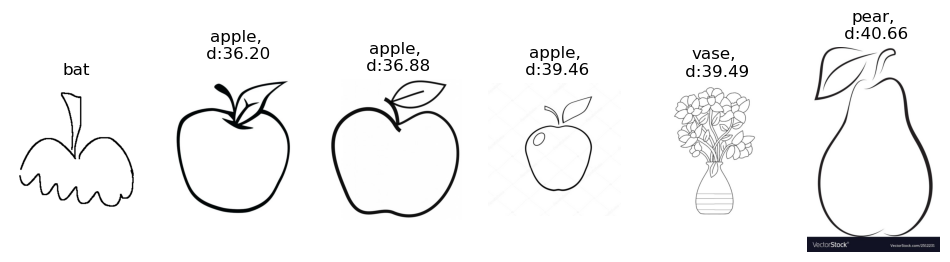
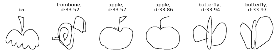
(b) Bat, recognised incorrectly (testing, sketch $\rightarrow$ quickdraw), left: sketch, right: quickdraw

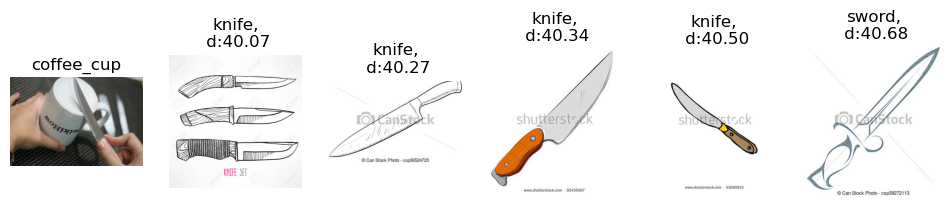
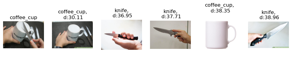
(c) Coffee cup (testing, sketch $\rightarrow$ real), left: sketch, right: real

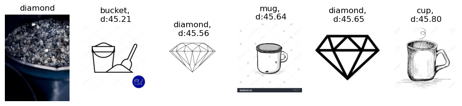
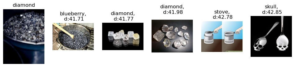
(d) Diamond, recognised incorrectly (testing, sketch $\rightarrow$ real), left: sketch, right: real

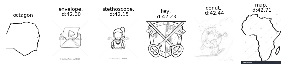
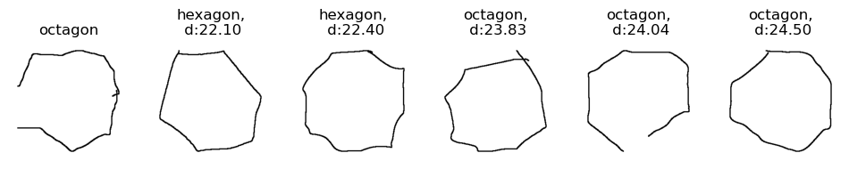
(e) Octagon, recognised incorrectly (testing, sketch $\rightarrow$ quickdraw), left: sketch, right: quickdraw

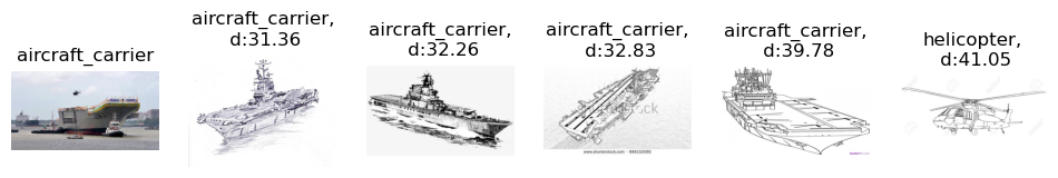
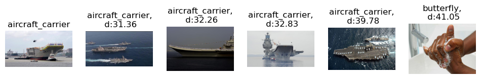
(f) Aircraft carrier (testing, sketch $\rightarrow$ real), left: sketch, right: real prototypes

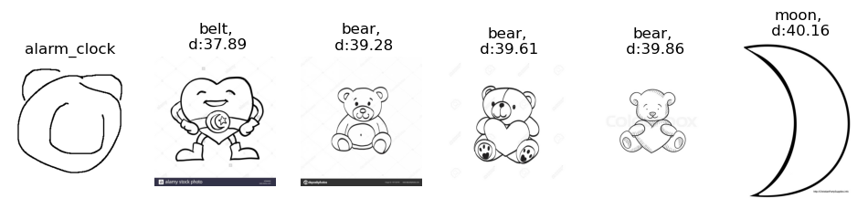
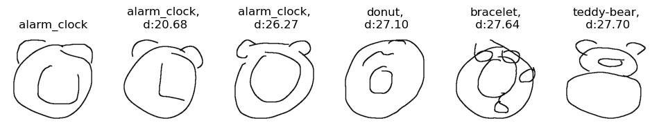
(g) Alarm clock (testing, sketch $\rightarrow$ quickdraw), left: sketch prototypes, right: quickdraw prototypes

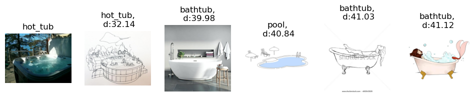
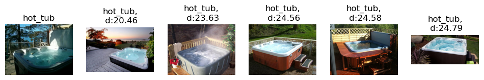
(h) Hot tub (testing, sketch $\rightarrow$ real), left: sketch prototypes, right: real prototypes

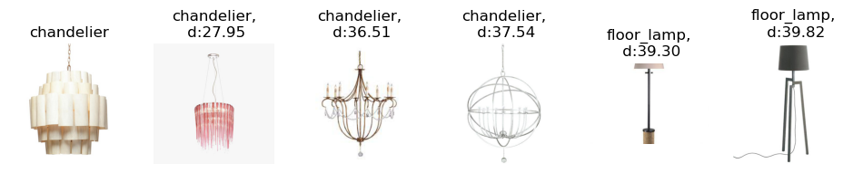
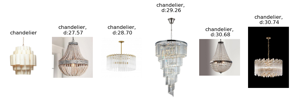
(i) Chandelier (training, sketch $\rightarrow$ real), left: sketch prototypes, right: real prototypes

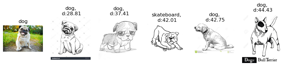
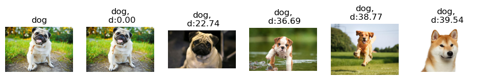
(j) Dog (training, sketch $\rightarrow$ real), left: sketch prototypes, right: real prototypes

Figure 3: Interpretations of decision making through closest prototypes (the leftmost images are queries, and the further ones are prototypes)

To better understand the performance scores, we provide visualisation for nearest prototypes for the ViT-SWAG, finetuned on ImageNet-1K ((see Figure 3). For the same latent space, this numerical estimate can be compared like-for-like between different examples and datasets.

One can see from Figure 3, that in many cases, even for the incorrect classification, the closest examples make semantic sense. In Figure 3(f), the model successfully relates aircraft carriers in different poses, sketched or photographed. The alarm clock (Figure 3(g)) recognises the quickdraw prototypes, but struggles to generalise to the sketch prototypes. Angel quickdraw prototypes (see Figure 3(a) ) show confusion (in the quickdraw domain) between similarly-looking angels, spiders and bats. The results are worse for cross-domain examples. The quickdraw sample in Figure 3(b), supposed to be a bat, looks indeed much like an apple. This is duly reflected by the model outputs. Coffee cup example (see Figure 3(c)), demonstrates competition between the coffee cup and the knife prototypes as the image contains both. Seeing the nearest blueberry example to the real diamond query image (see Figure 3(d)) helps make sense out of the incorrect recognition. In the hot tub example (Figure 3(h)), one can see that the varieties of appearances of the same objects are shown to have a low distance. The feature space also places closer different types of light fixtures, as one can see in Figure 3(i), in sketch and real domains alike.The limitations of differentiating between geometric figures such as hexagons and octagons (see Figure 3(e) suggest that despite generality, textural information often trumps the semantic one. For the dogs scenario on training data (see Figure 3(j), one can see that while the model has sometimes advantage to find the exact match with the prototypes, it also shows remarkable cross-domain generalisation.

References

- Angelov & Soares (2020) Plamen Angelov and Eduardo Soares. Towards explainable deep neural networks (xdnn). Neural Networks, 130:185–194, 2020.
- Angelov et al. (2023) Plamen Angelov, Dmitry Kangin, and Ziyang Zhang. Towards interpretable-by-design deep learning algorithms. arXiv preprint arXiv:2311.11396, 2023.
- Böhle et al. (2022) Moritz Böhle, Mario Fritz, and Bernt Schiele. B-cos networks: Alignment is all we need for interpretability. In Proceedings of the IEEE/CVF Conference on Computer Vision and Pattern Recognition, pp. 10329–10338, 2022.
- Chen et al. (2019) Chaofan Chen, Oscar Li, Daniel Tao, Alina Barnett, Cynthia Rudin, and Jonathan K Su. This looks like that: deep learning for interpretable image recognition. Advances in neural information processing systems, 32, 2019.
- Dai et al. (2021) Yin Dai, Yifan Gao, and Fayu Liu. Transmed: Transformers advance multi-modal medical image classification. Diagnostics, 11(8):1384, 2021.
- Dosovitskiy et al. (2021) Alexey Dosovitskiy, Lucas Beyer, Alexander Kolesnikov, Dirk Weissenborn, Xiaohua Zhai, Thomas Unterthiner, Mostafa Dehghani, Matthias Minderer, Georg Heigold, Sylvain Gelly, Jakob Uszkoreit, and Neil Houlsby. An image is worth 16x16 words: Transformers for image recognition at scale. In International Conference on Learning Representations, 2021. URL https://openreview.net/forum?id=YicbFdNTTy.
- He et al. (2016) Kaiming He, Xiangyu Zhang, Shaoqing Ren, and Jian Sun. Deep residual learning for image recognition. In Proceedings of the IEEE conference on computer vision and pattern recognition, pp. 770–778, 2016.
- Liu et al. (2021a) Xiaofeng Liu, Zhenhua Guo, Site Li, Fangxu Xing, Jane You, C-C Jay Kuo, Georges El Fakhri, and Jonghye Woo. Adversarial unsupervised domain adaptation with conditional and label shift: Infer, align and iterate. In Proceedings of the IEEE/CVF international conference on computer vision, pp. 10367–10376, 2021a.
- Liu et al. (2021b) Ze Liu, Yutong Lin, Yue Cao, Han Hu, Yixuan Wei, Zheng Zhang, Stephen Lin, and Baining Guo. Swin transformer: Hierarchical vision transformer using shifted windows. In Proceedings of the IEEE/CVF international conference on computer vision, pp. 10012–10022, 2021b.
- Oquab et al. (2023) Maxime Oquab, Timothée Darcet, Théo Moutakanni, Huy Vo, Marc Szafraniec, Vasil Khalidov, Pierre Fernandez, Daniel Haziza, Francisco Massa, Alaaeldin El-Nouby, et al. Dinov2: Learning robust visual features without supervision. arXiv preprint arXiv:2304.07193, 2023.
- Peng et al. (2019) Xingchao Peng, Qinxun Bai, Xide Xia, Zijun Huang, Kate Saenko, and Bo Wang. Moment matching for multi-source domain adaptation. In Proceedings of the IEEE/CVF international conference on computer vision, pp. 1406–1415, 2019.
- Saenko et al. (2010) Kate Saenko, Brian Kulis, Mario Fritz, and Trevor Darrell. Adapting visual category models to new domains. In Computer Vision–ECCV 2010: 11th European Conference on Computer Vision, Heraklion, Crete, Greece, September 5-11, 2010, Proceedings, Part IV 11, pp. 213–226. Springer, 2010.
- Saito et al. (2018) Kuniaki Saito, Kohei Watanabe, Yoshitaka Ushiku, and Tatsuya Harada. Maximum classifier discrepancy for unsupervised domain adaptation. In Proceedings of the IEEE conference on computer vision and pattern recognition, pp. 3723–3732, 2018.
- Selvaraju et al. (2017) Ramprasaath R Selvaraju, Michael Cogswell, Abhishek Das, Ramakrishna Vedantam, Devi Parikh, and Dhruv Batra. Grad-cam: Visual explanations from deep networks via gradient-based localization. In Proceedings of the IEEE international conference on computer vision, pp. 618–626, 2017.
- Simonyan et al. (2014) K Simonyan, A Vedaldi, and A Zisserman. Deep inside convolutional networks: visualising image classification models and saliency maps. In Proceedings of the International Conference on Learning Representations (ICLR). ICLR, 2014.
- Singh et al. (2022) Mannat Singh, Laura Gustafson, Aaron Adcock, Vinicius de Freitas Reis, Bugra Gedik, Raj Prateek Kosaraju, Dhruv Mahajan, Ross Girshick, Piotr Dollár, and Laurens Van Der Maaten. Revisiting weakly supervised pre-training of visual perception models. In Proceedings of the IEEE/CVF Conference on Computer Vision and Pattern Recognition, pp. 804–814, 2022.
- Snell et al. (2017) Jake Snell, Kevin Swersky, and Richard Zemel. Prototypical networks for few-shot learning. Advances in neural information processing systems, 30, 2017.
- Tzeng et al. (2017) Eric Tzeng, Judy Hoffman, Kate Saenko, and Trevor Darrell. Adversarial discriminative domain adaptation. In Proceedings of the IEEE conference on computer vision and pattern recognition, pp. 7167–7176, 2017.
- Vaswani et al. (2017) Ashish Vaswani, Noam Shazeer, Niki Parmar, Jakob Uszkoreit, Llion Jones, Aidan N Gomez, Łukasz Kaiser, and Illia Polosukhin. Attention is all you need. Advances in neural information processing systems, 30, 2017.
- Zellinger et al. (2017) Werner Zellinger, Thomas Grubinger, Edwin Lughofer, Thomas Natschläger, and Susanne Saminger-Platz. Central moment discrepancy (cmd) for domain-invariant representation learning. arXiv preprint arXiv:1702.08811, 2017.
- Zhang et al. (2022) Chongzhi Zhang, Mingyuan Zhang, Shanghang Zhang, Daisheng Jin, Qiang Zhou, Zhongang Cai, Haiyu Zhao, Xianglong Liu, and Ziwei Liu. Delving deep into the generalization of vision transformers under distribution shifts. In Proceedings of the IEEE/CVF conference on Computer Vision and Pattern Recognition, pp. 7277–7286, 2022.
- Zhao et al. (2018) Han Zhao, Shanghang Zhang, Guanhang Wu, Joao P Costeira, José MF Moura, and Geoffrey J Gordon. Multiple source domain adaptation with adversarial learning. 2018.