On Identification of Dynamic Treatment Regimes with Proxies of Hidden Confounders

Abstract

We consider identification of optimal dynamic treatment regimes in a setting where time-varying treatments are confounded by hidden time-varying confounders, but proxy variables of the unmeasured confounders are available. We show that, with two independent proxy variables at each time point that are sufficiently relevant for the hidden confounders, identification of the joint distribution of counterfactuals is possible, thereby facilitating identification of an optimal treatment regime.

1 Introduction

Estimating single time point optimal treatment regimes and multiple time point dynamic treatment regimes has received much attention in a diverse array of fields, including biostatistics, computer science, and economics. When data are obtained from a randomized controlled trial, A/B test, or a sequential multiple assignment randomized trial (SMART), the assumptions required for identification and estimation of optimal rules/regimes can be met by design. Alternatively, when one wishes to estimate the optimal regime from observational data, unverifiable assumptions such as the no unmeasured confounding assumption (NUCA) is typically invoked in point exposure settings and its time-varying analog termed sequential randomization assumption (SRA) is likewise invoked in time-varying treatment settings (Robins (1986), Murphy (2003)). In this article, we do not assume that experimental data are available, e.g. SMARTs, nor do we impose SRA. Instead, we allow for confounding by hidden factors for which variables with special causal structure, called proxies, are available, which we leverage to identify an optimal dynamic treatment regime in an observational study. Our results are also relevant beyond observational studies, as even when treatment assignment is randomized, there often is noncompliance. In a SMART with noncompliance, randomization can be viewed either as a valid instrumental variable, or alternatively as treatment confounding proxy, one of the two types of proxies we plan to leverage for identification.

1.1 Related Literature

There are several strands of research related to our work. The proximal causal inference framework, originally introduced in Miao et al. (2018) for the point exposure scenario, has been extended in many directions. Notably, Qi et al. (2023) and Shen and Cui (2022) solve the point exposure optimal treatment regime problem under unmeasured confounding using proxies. Proximal inference tools have also been applied to more complex regimes, such as mediation analysis, longitudinal studies, and off-policy evaluation in Tchetgen Tchetgen et al. (2024), Ying et al. (2023), Dukes et al. (2023), Singh (2021), Bennett and Kallus (2021), Miao et al. (2022), respectively. These works, similar to ours, require solving nested integral equations. In contrast, none require the challenging task of identifying the joint distribution of counterfactuals as a crucial step towards identifying an optimal dynamic regime, as Ying et al. (2023) only considers models for marginal counterfactual distributions indexed by static regimes, and Bennett and Kallus (2021) and Miao et al. (2022) study partially observed markov decision processes.

Alternatives to proximal causal inference with longitudinal data subject to unmeasured confounding include instrumental variable approaches as well as partial identification/sensitivity analysis approaches. Michael et al. (2023) study identification of a static regime using instrumental variables. Chen and Zhang (2023) study improvement of dynamic treatment regimes using instrumental variables given partial identification bounds, though they do not formally state how these should be obtained and the assumptions required. Han (2023) estimates a partial order of dynamic treatment regimes using an instrumental variable. Bruns-Smith and Zhou (2023) study robust Q-learning under a model analogous to the marginal sensitivity model of Tan (2006).

One recent work that achieves identification of optimal dynamic treatment regimes under unmeasured confounding is Han (2021), using instrumental variables in addition to structural assumptions grounded in econometrics. Aside from Han (2021), to the best of our knowledge, there do not exist general identification results for optimal dynamic treatment regimes in the presence of unmeasured confounding. We fill this gap by leveraging proxy variables under proxy relevance conditions formally known as completeness conditions, with similar characteristics as those in Ying et al. (2023).

2 Preliminaries

2.1 Notation

To simplify the exposition, we consider a two time point setting, though the results can be extended to any finite number of time points as shown in the Appendix. We suppose the data contains $n$ iid draws of a random vector $(U_{0},Y_{0},Z_{1},A_{1},W_{1},U_{1},Y_{1},Z_{2},A_{2},W_{2},Y_{2})$. Here, the $A$ variables are treatments, $U_{0}$ and $U_{1}$ represent time-varying unmeasured confounders of the effects of $(A_{1},A_{2})$, $Y_{0}$ is a baseline measurement of the outcome which may also confound the effect of subsequent treatments, $Y_{1}$ and $Y_{2}$ are post-treatment outcome measurements, and $Z$ and $W$ are proxies, whose causal structure is introduced in the next section. The overarching goal is to identify the optimal treatment regime based on past treatments and outcomes. In the two time point setting, we consider regimes at time point 2, ($d_{2}=d_{2}(y_{1},a_{1},y_{0})$) that depend on past outcomes, and treatment; and at time point 1 ($d_{1}=d_{1}(y_{0})$) that depend on the pretreatment outcome measurement. We note that allowing the $Y$ outcome process to be multivariate poses no additional theoretical difficulty, though the proxy conditions we introduce later would need to apply to these multivariate outcomes. We focus on the univariate outcome case to simplify the exposition. We formalize the framework in Section 3. We use the summation notation $\sum$, which in a slight abuse of notation, can also be interpreted as integrals for continuous variables. Also, we adopt the convention that uppercase variables denote random variables and lower case denote realizations of a random variable. At times, we write $f(a)$ instead of $f(A=a)$ to represent the density or probability mass function of random variable $A$ evaluated at $a$, but the abbreviation will be clear from context. E denotes the expectation operator. Finally, we adopt the $\overline{A}_{k}$ notation to represent a random variable and all its predecessors, i.e. $\overline{A}_{k}=(A_{1},\ldots,A_{k})$ or $\overline{A}_{k}=(A_{0},A_{1},\ldots,A_{k})$.

2.2 Assumptions

We next introduce formal causal assumptions underlying the data. First, we assume potential outcomes $Y_{2}(a_{1},a_{2})$ and $Y_{1}(a_{1})$ are well-defined and there is no interference, such that the former represents a unit’s outcome had, possibly contrary to fact, its treatment history been set to $(a_{1},a_{2})$; the latter is likewise defined. We also make the standard consistency assumption, so that $Y_{2}=Y_{2}(A_{1},A_{2})$ and $Y_{1}=Y_{1}(A_{1})$. Key to the approach is an assumption that the unobserved factors $U_{0},U_{1}$ would in principle suffice to account for time-varying confounding which we formalize as follows.

Assumption 1 (Sequential Proximal Latent Randomization Assumption).

$$\{Y_{2}\left(a_{1},a_{2}\right),\overline{W}_{2}\}\perp\!\!\!\perp\{A_{2},\overline{Z}_{2}\}|\left(\overline{U}_{1},\overline{Y}_{1},A_{1}=a_{1}\right)$$

$$\left\{{Y}_{1}\left(a_{1}\right),Y_{2}\left(a_{1},a_{2}\right),W_{1}\right\}\perp\!\!\!\perp\{A_{1},Z_{1}\}|\left(U_{0},Y_{0}\right)$$

$$\{\overline{W}_{2},Y_{1}\}\perp\!\!\!\perp Z_{1}\mid A_{1},U_{0},Y_{0}.$$

The first two lines of the assumption correspond to the assumptions from Ying et al. (2023); specifically Equations 2-4. The third assumption is an additional assumption that requires that $Z_{1}$ has no direct effect on $W_{2}$. The canonical situation where these conditions might be expected to hold would be when $W_{1}$ and $W_{2}$ are negative control outcomes and $Z_{1}$ and $Z_{2}$ are negative control exposures. In other words, $A_{1}$ and $A_{2}$ do not have direct effects on $W_{1}$ and $W_{2}$, respectively and $Z_{1}$ and $Z_{2}$ do not have direct effects on $Y_{1}$ and $Y_{2}$, respectively. In addition, $Z$ and $W$ should not affect each other. Note that Assumption 1 does not preclude $A_{1}$ from having an effect on $W_{2}$. A DAG that satisfies Assumption 1 is depicted in Figure 1 below. This DAG is similar to the one depicted in Figure 2 of Ying et al. (2023), with the addition of a pre-treatment confounder $Y_{0}$ and an intermediate outcome $Y_{1}$. The $Y$ in that DAG corresponds to $Y_{2}$ in Figure 1. The $Y_{0},U_{0}$ and $Y_{1},U_{1}$ are grouped together in a single node for increased readability, and represents that they have the same parent and child nodes. Previously, Tchetgen Tchetgen et al. (2024) and Ying et al. (2023) reanalyzed a study of the effect of an anti-rheumatic therapy called Methotrexate (MTX) on average number of tender joints at end of follow-up among patients with rheumatoid arthritis. They utilized erythrocyte sedimentation rate as a negative control exposure and patient’s global assessment as a negative control outcome. More generally, good candidates for negative control exposures include randomization in a SMART with noncompliance, or a time-varying instrumental variable in a longitudinal observational study. For more examples of both types of proxy variables, we refer the reader to Shi et al. (2020b).

Figure 1: An example of a DAG where Assumption 1 holds.

3 Proximal Identification

3.1 Characterizing the optimal regime

We wish to solve the following optimal treatment regime problem. In particular, the goal is to identify $d_{2}^{opt}(\overline{Y}_{1},\overline{A}_{1})$ and $d_{1}^{opt}(Y_{0})$ that solve

$$d_{2}^{opt}(\overline{Y}_{1},\overline{A}_{1}),d_{1}^{opt}(Y_{0})\in\underset{d_{1},d_{2}}{\arg\max}\ {E}\left\{Y_{2}\left(d_{1}(Y_{0}),d_{2}(Y_{1},A_{1},Y_{0})\right)\right\}.$$

In other words, we seek to find the regime at time point 1 based on a baseline outcome $Y_{0}$ and regime at time point 2 based on a baseline outcome measurement $Y_{0}$, previous treatment $A_{1}$, and previous outcome $Y_{1}$ that will maximize the final outcome $Y_{2}$. We refer to ${E}\left\{Y_{2}\left(d_{1}(Y_{0}),d_{2}(Y_{1},A_{1},Y_{0})\right)\right\}$ as the value of a regime $(d_{1},d_{2})$. The regret of an estimated regime is the value of the optimal regime minus the value of the estimated regime. We point out that maximizing the final outcome is without loss of generality, as the intermediate potential outcomes $Y_{1}(a_{1})$ can be used in defining the value function (see Chapter 6.2.1 of Tsiatis et al. (2019) for a detailed discussion). It is well-known that $d_{1}^{opt}$ and $d_{2}^{opt}$ have the following equivalent and more convenient characterizations (e.g. Chapter 7.2 of Tsiatis et al. (2019) ):

$$d_{2}^{opt}\left(\overline{y}_{1},a_{1}\right) =\underset{a_{2}}{\arg\max}\ {E}\left\{Y_{2}\left(a_{1},a_{2}\right)|\overline{Y}_{1}\left(a_{1}\right)=\overline{y}_{1}\right\}$$ (1)

$$V_{2}^{opt}\left(a_{1},\overline{y}_{1}\right) =\underset{a_{2}}{\max}\ {E}\left\{Y\left(a_{1},a_{2}\right)|\overline{Y}_{1}\left(a_{1}\right)=\overline{y}_{1}\right\}$$

$$d_{1}^{opt}\left(y_{0}\right) =\underset{a_{1}}{\arg\max}\ {E}\left\{V_{2}^{opt}\left(a_{1},Y_{1}\left(a_{1}\right),Y_{0}\right)|Y_{0}=y_{0}\right\}.$$

Note that

$${E}\left\{Y_{2}\left(a_{1},a_{2}\right)|\overline{Y}_{1}\left(a_{1}\right)=\overline{y}_{1}\right\}=\sum_{y_{2}}\frac{f\left(Y_{2}\left(a_{1},a_{2}\right)=y_{2},Y_{1}\left(a_{1}\right)=y_{1}|y_{0}\right)}{f\left(Y_{1}\left(a_{1}\right)=y_{1}|y_{0}\right)}y_{2},\ \text{ and }$$

$${E}\left\{V_{2}\left(a_{1},Y_{1}\left(a_{1}\right),Y_{0}\right)|Y_{0}=y_{0}\right\}=\sum_{y_{1}}V_{2}(a_{1},y_{1},y_{0})f\left(Y_{1}\left(a_{1}\right)=y_{1}|y_{0}\right),$$

which clearly indicates that the quantities $f\left(Y_{2}\left(a_{1},a_{2}\right)=y_{2},Y_{1}\left(a_{1}\right)=y_{1}|y_{0}\right)$ and $f\left(Y_{1}\left(a_{1}\right)=y_{1}|y_{0}\right)$ are crucial for identification of the optimal regime. Note that the task of identifying optimal regimes in multiple time points is markedly distinct from and more difficult than identification of optimal regimes in the single time point case. This is due to the fact that to identify the optimal regime requires identification of the joint distribution of the counterfactuals $(Y_{2}(a_{1},a_{2}),Y_{1}(a_{1}))$. Previous work for observational longitidunal studies such as Michael et al. (2023) and Ying et al. (2023) provide identification results for functionals of the marginal distribution of the single counterfactual $Y_{2}(a_{1},a_{2})$ for some fixed $a_{1},a_{2}$, but not the joint $(Y_{2}(a_{1},a_{2}),Y_{1}(a_{1}))$. By the latent SRA, i.e. Assumption 1, the joint density of the counterfactuals can be written in terms of observable and the unmeasured confounders by a standard application of Robins’ g-formula. Unfortunately, without access to the unmeasured confounders, we must resort to alternative assumptions for identification.

3.2 Main Result

Identification of the optimal regime is based on the existence of solutions to certain carefully defined integral equations. Explicitly, we assume the following:

Assumption 2 (Time-varying Bridge Functions).

There exist functions $h_{22}\left(\overline{y}_{2},\overline{w}_{2},\overline{a}_{2}\right)$ and $h_{21}\left(\overline{y}_{1},w_{1},\overline{a}_{2}\right)$ that satisfy

$$f\left(Y_{2}=y_{2}|\overline{y}_{1},\overline{u}_{1},\overline{a}_{2}\right)=\sum_{\overline{w}_{2}}h_{22}\left(\overline{y}_{2},\overline{w}_{2},\overline{a}_{2}\right)f\left(\overline{w}_{2}|\overline{y}_{1},\overline{a}_{2},\overline{u}_{1}\right),$$

and

$$\sum_{\overline{w}_{2}}h_{22}\left(\overline{y}_{2},\overline{w}_{2},\overline{a}_{2}\right)f(y_{1}|y_{0},u_{0},a_{1})f\left(\overline{w}_{2}|\overline{y}_{1},a_{1},u_{0}\right)=\sum_{w_{1}}h_{21}\left(\overline{y}_{2},w_{1},\overline{a}_{2}\right)f\left(w_{1}|y_{0},a_{1},u_{0}\right),$$

respectively.

The integral equation involving the $h_{22}$ function is similar to previous integral equations in the proxy literature (Miao et al., 2018; Ying et al., 2023; Tchetgen Tchetgen et al., 2024), with the left hand side being a conditional density given unmeasured confounders while the right hand side is a conditional mean function. Meanwhile, the integral equation involving $h_{21}$, to the best of our knowledge, has no precedent in the current literature. Rearranging the integral equation, we obtain

$$f(y_{1}|y_{0},u_{0},a_{1})=\left.\sum_{w_{1}}h_{21}\left(\overline{y}_{2},w_{1},\overline{a}_{2}\right)f\left(w_{1}|y_{0},a_{1},u_{0}\right)\middle/\sum_{\overline{w}_{2}}h_{22}\left(\overline{y}_{2},\overline{w}_{2},\overline{a}_{2}\right)f\left(\overline{w}_{2}|\overline{y}_{1},a_{1},u_{0}\right)\right..$$

This looks somewhat familiar, as the left hand side is a conditional density including the first unmeasured confounder, while the right hand side is the ratio of two conditional expectations, but the numerator is only conditional on $(y_{0},a_{1},u_{0})$ with randomness over $W_{1}$ while the denominator is conditional on $(y_{1},y_{0},a_{1},u_{0})$ with randomness over $(W_{1},W_{2})$. We can now state our main result relating the joint and marginal counterfactual densities to the $h_{21}$ function.

Theorem 1.

Under Assumptions 1 and 2

$$f\left(Y_{2}\left(a_{1},a_{2}\right)=y_{2},Y_{1}\left(a_{1}\right)=y_{1}|y_{0}\right)=\sum_{w_{1}}h_{21}\left(\overline{y}_{2},w_{1},\overline{a}_{2}\right)f\left(w_{1}|y_{0}\right)\text{ and }$$ (2)

$$f\left(Y_{1}\left(a_{1}\right)=y_{1}|y_{0}\right)=\sum_{y_{2}}\sum_{w_{1}}h_{21}\left(\overline{y}_{2},w_{1},\overline{a}_{2}\right)f\left(w_{1}|y_{0}\right).$$ (3)

Assumption 2 requires the existence of solutions to integral equations involving the unmeasured confounders. Thus, without additional assumptions, the functions $h_{22}$, $h_{21}$ are not identified from the observed data. We next introduce conditions under which identification is possible.

Assumption 3 (Completeness/Relevance).

For any square integrable $g_{1}$, we have that

$${E}[g_{1}(\overline{U}_{1})\mid\overline{y}_{1},\overline{z}_{2},\overline{a}_{2}]=0\text{ implies }g_{1}(\overline{U}_{1})=0.$$

In addition, for any square integrable $g_{0}$, we have that

$${E}[g_{0}({U}_{0})\mid{y}_{0},{z}_{1},{a}_{1}]=0\text{ implies }g_{0}({U}_{0})=0.$$

Completeness roughly requires that any variability in the unmeasured confounders $U$ induces some variability in $Z$. If all variables are discrete, Assumption 3 requires that $\text{dim}(\bar{u}_{1})\leq\text{dim}(\bar{z}_{2})$ and $\text{dim}({u}_{0})\leq\text{dim}({z}_{1})$.

Lemma 1.

Suppose there exist $h_{22}\left(\overline{y}_{2},\overline{w}_{2},\overline{a}_{2}\right)$ and $h_{21}\left(\overline{y}_{1},w_{1},\overline{a}_{2}\right)$ that satisfy

$$f\left(Y_{2}=y_{2}|\overline{y}_{1},\overline{z}_{2},\overline{a}_{2}\right) =\sum_{\overline{w}_{2}}h_{22}\left(\overline{y}_{2},\overline{w}_{2},\overline{a}_{2}\right)f\left(\overline{w}_{2}|\overline{y}_{1},\overline{a}_{2},\overline{z}_{2}\right)$$ (4)

$$\sum_{\overline{w}_{2}}h_{22}\left(\overline{y}_{2},\overline{w}_{2},\overline{a}_{2}\right)f(y_{1}|y_{0},z_{1},a_{1})f\left(\overline{w}_{2}|\overline{y}_{1},a_{1},z_{1}\right) =\sum_{w_{1}}h_{21}\left(\overline{y}_{2},w_{1},\overline{a}_{2}\right)f\left(w_{1}|y_{0},a_{1},z_{1}\right).$$

respectively. If Assumption 3 also holds, then $h_{22}$ and $h_{21}$ also solve the latent integral equations from Assumption 2.

Lemma 1 gives a characterization of the bridge functions in terms of observable variables rather than the latent variables as in Assumption 2. Equipped with this result, identification of the optimal regime is possible if one can find $h_{22}\left(\overline{y}_{2},\overline{w}_{2},\overline{a}_{2}\right)$, $h_{21}\left(\overline{y}_{1},w_{1},\overline{a}_{2}\right)$, that satisfy

$$f\left(Y_{2}=y_{2}|\overline{y}_{1},\overline{a}_{2},\overline{z}_{2}\right) =\sum_{\overline{w}_{2}}h_{22}\left(\overline{y}_{2},\overline{w}_{2},\overline{a}_{2}\right)f\left(\overline{w}_{2}|\overline{y}_{1},\overline{a}_{2},\overline{z}_{2}\right),$$

$$\sum_{\overline{w}_{2}}h_{22}\left(\overline{y}_{2},\overline{w}_{2},\overline{a}_{2}\right)f\left(\overline{w}_{2}|\overline{y}_{1},a_{1},z_{1}\right)f(y_{1}|y_{0},\ a_{1},z_{1}) =\sum_{w_{1}}h_{21}\left(\overline{y}_{2},w_{1},\overline{a}_{2}\right)f\left(w_{1}|y_{0},a_{1},z_{1}\right).$$

We note that uniqueness of solutions to the above equations is not necessary for identification of the optimal regime; any solutions suffice. We outline primitive conditions for the existence (and uniqueness) of solutions to integral equations in Section B of the supplementary material. Theorem 1 and Lemma 1 establish that the optimal rules/values at time points 2 and 1 are identified using only observed data as described in the following corollary.

Corollary 1.

Under Assumptions 1, 3, and given functions $h_{22}$ and $h_{21}$ that satisfy Equation 4, the optimal regime can be characterized as follows:

$$d_{2}^{opt}\left(\overline{y}_{1},a_{1}\right) =\underset{a_{2}}{\arg\max\ }{E}\left\{Y_{2}\left(a_{1},a_{2}\right)|\overline{Y}_{1}\left(a_{1}\right)=\overline{y}_{1}\right\}$$

$$=\underset{a_{2}}{\arg\max}\sum_{y_{2}}\frac{\sum_{w_{1}}h_{21}\left(\overline{y}_{2},w_{1},\overline{a}_{2}\right)f\left(w_{1}|y_{0}\right)}{\sum_{y_{2}}\sum_{w_{1}}h_{21}\left(\overline{y}_{2},w_{1},\overline{a}_{2}\right)f\left(w_{1}|y_{0}\right)}y_{2},$$

$$V_{2}^{opt}\left(a_{1},\overline{y}_{1}\right) =\underset{a_{2}}{\max\ }{E}\left\{Y\left(a_{1},a_{2}\right)|\overline{Y}_{1}\left(a_{1}\right)=\overline{y}_{1}\right\}$$

$$=\underset{a_{2}}{\max}\sum_{y_{2}}\frac{\sum_{w_{1}}h_{21}\left(\overline{y}_{2},w_{1},\overline{a}_{2}\right)f\left(w_{1}|y_{0}\right)}{\sum_{y_{2}}\sum_{w_{1}}h_{21}\left(\overline{y}_{2},w_{1},\overline{a}_{2}\right)f\left(w_{1}|y_{0}\right)}y_{2},$$

$$d_{1}^{opt}\left(y_{0}\right) =\underset{a_{1}}{\arg\max\ }{E}\left\{V_{2}^{opt}\left(a_{1},Y_{1}\left(a_{1}\right),Y_{0}\right)|Y_{0}=y_{0}\right\}$$

$$=\underset{a_{1}}{\arg\max}\sum_{y_{1}}\sum_{y_{2}}\sum_{w_{1}^{*}}h_{21}\left(\overline{y}_{2},w_{1}^{*},\overline{a}_{2}\right)f\left(w_{1}^{*}|y_{0}\right)V_{2}^{opt}\left(a_{1},\overline{y}_{1}\right).$$

In principle, Corollary 1 can be used to estimate the optimal dynamic treatment regime. However, in the general case, the bridge functions can be challenging to estimate and compute nonparametrically as they may involve (conditional) densities. In particular, $h_{21}$’s nontrivial dependence on $h_{22}$ is distinct from other bridge functions in the literature (Ying et al., 2023; Tchetgen Tchetgen et al., 2024). In Section 4 below, we consider a setting only involving categorical variables as an initial crucial step towards inference in this challenging setting. Inference in the continuous case will be considered elsewhere given the significant challenges it presents.

3.3 A connection to the single time-point setting

In the single time-point setting, a single integral equation needs to be solved Miao et al. (2018), rather than nested ones. Specifically, Miao et al. (2018) require the existence of a function $h_{11}\left(w_{1},\overline{y}_{1},a_{1}\right)$ that solves the following so-called Fredholm integral equation of the first kind:

$$f\left(Y_{1}=y_{1}|y_{0},a_{1},u_{0}\right)=\sum_{w_{1}}h_{11}\left(w_{1},\overline{y}_{1},a_{1}\right)f\left(w_{1}|u_{0},y_{0}\right).$$ (5)

Miao et al. (2018) show that $f\left(Y_{1}(a_{1})=y_{1}|y_{0}\right)=\sum_{w_{1}}h_{11}\left(w_{1},\overline{y}_{1},a_{1}\right)f\left(w_{1}|y_{0}\right)$ for any $h_{11}$ that solves Equation 5. Thus, in principle, we could solve for such an $h_{11}$ directly. It turns out that $h_{21}$ is related to $h_{11}$. We establish this relationship in the proposition below.

Proposition 1.

For any $h_{21}$ that satisfies the conditions in Assumption 2, the function $\sum_{y_{2}}h_{21}(\overline{y}_{2},w_{1},\overline{a}_{2})$ solves Equation 5.

From Proposition 1, we see that in principle, it does not make a difference whether we marginalize $h_{21}$ over $y_{2}$ to identify the single counterfactual law $f(Y_{1}(a_{1})=y_{1}\mid y_{0})$ or identify it using $h_{11}$ directly from Equation 5.

4 Categorical Variables

4.1 Closed form expressions and estimation

In this section, we consider in detail the canonical case where variables $U_{t-1}$, $W_{t}$ and $Z_{t}$ are categorical with $|W_{t}|=|Z_{t}|=|U_{t-1}|=k$, so that all proxies and unmeasured confounders have the same cardinality. Assuming equal cardinality is restrictive, however it is particularly instructive as identifying assumptions are easier to interpret and explicit simple closed-form expressions to the integral equations can be obtained which simplifies estimation of the optimal regime. In Section D of the supplementary material, we consider the more general setting where $\min(|W_{t}|,|Z_{t}|)\geq|U_{t-1}|$, which appears to be necessary for nonparametric identification, whereby the cardinality of hidden factors $U$ must not exceed that of proxies. Throughout, we suppose that the treatment at each time point is binary, $|A_{t}|=2$. We proceed similarly to Shi et al. (2020a) with the following notation: we write $P(W\mid u)=\left\{\operatorname{pr}\left(w_{1}\mid u\right),\ldots,\operatorname{pr}\left(w_{k}\mid u\right)\right\}^{\mathrm{T}},P(w\mid$ $U)=\left\{\operatorname{pr}\left(w\mid u_{1}\right),\ldots,\operatorname{pr}\left(w\mid u_{k}\right)\right\}$ and $P(W\mid U)=\left\{P\left(W\mid u_{1}\right),\ldots,P\left(W\mid u_{k}\right)\right\}$ for a column vector, a row vector and a matrix, respectively, that consist of conditional probabilities $\operatorname{pr}(w\mid u)$. For all other variables, vectors and matrices consisting of conditional probabilities are analogously defined. Specifically, $P(U\mid$ $z,x)=\left\{\operatorname{pr}\left(u_{1}\mid z,x\right),\ldots,\operatorname{pr}\left(u_{k}\mid z,x\right)\right\}^{\mathrm{T}}$, $P(U\mid Z,x)=\left\{P\left(U\mid z_{1},x\right),\ldots,P\left(U\mid z_{k},x\right)\right\}$, and $P(y\mid Z,x)=$ $\left\{\operatorname{pr}\left(y\mid z_{1},x\right),\ldots,\operatorname{pr}\left(y\mid z_{k},x\right)\right\}$. Interestingly, as pointed out in Miao et al. (2018), a key simplification that occurs in the categorical case is that the completeness condition reduces to a rank condition, which under the equal cardinality condition, amounts to invertibility of certain key matrices.

Assumption 4 (Invertibility).

For all $(\overline{y}_{1},\overline{a}_{2})$, the matrices $P(\overline{W}_{2}\mid\overline{U}_{1},\overline{y}_{1},\overline{a}_{2})$ and $P(\overline{U}_{1}\mid\overline{Z}_{2},\overline{y}_{1},\overline{a}_{2})$ are invertible. In addition, for all $({y}_{0},{a}_{1})$, $P({W}_{1}\mid{U}_{0},{y}_{0},{a}_{1})$ and $P({U}_{1}\mid{Z}_{1},{y}_{0},{a}_{1})$ are invertible.

These invertibility assumptions require that the corresponding matrices are full rank. We can now state a result about identification of $f(Y_{2}(a_{1},a_{2})=y_{2},Y_{1}(a_{1})=y_{1}\mid y_{0})$ and $f(Y_{1}(a_{1})=y_{1}\mid y_{0})$ in the categorical setting.

Proposition 2.

Let the cardinality of each of the $U$, $Z$, and $W$ variables equal $k$ for $2\leq k<\infty$. Also, suppose that Assumptions 1 and 4 hold. Then

$$f(Y_{2}(a_{1},a_{2})=y_{2},Y_{1}(a_{1})=y_{1}\mid y_{0})$$

$$=P(y_{2}\mid\overline{Z}_{2},\overline{y}_{1},\overline{a}_{2})P(\overline{W}_{2}\mid\overline{Z}_{2},\overline{y}_{1},\overline{a}_{2})^{-1}P(\overline{W}_{2},y_{1}\mid Z_{1},y_{0},a_{1})P(W_{1}\mid Z_{1},y_{0},a_{1})^{-1}P(W_{1}\mid y_{0}),\text{ and}$$

$$f(Y_{1}(a_{1})=y_{1}\mid y_{0})$$

$$=P(y_{1}\mid\overline{Z}_{1},\overline{y}_{0},\overline{a}_{1})P(W_{1}\mid Z_{1},y_{0},a_{1})^{-1}P(W_{1}\mid y_{0}).$$

Given the proceeding developments, simple substitution estimators are immediate. In fact, one may simply replace unknown population probabilities with empirical estimates. Then following the above, one obtains plug-in estimators $\widehat{f}(Y_{2}(a_{1},a_{2})=y_{2},Y_{1}(a_{1})=y_{1}\mid y_{0})$ and $\widehat{f}(Y_{1}(a_{1})=y_{1}\mid y_{0})$. Using these plug-in estimators, one then can find the treatment values maximizing corresponding value function (or minimizing regret) by appealing to Equation 1. In turn, one obtains estimates of the optimal treatment strategy at both time steps for any combination of histories of outcome and treatment variable. Stated explicitly:

$$\widehat{d}_{2}^{proxy}\left(\overline{y}_{1},a_{1}\right)$$

$$=\underset{a_{2}}{\arg\max}\sum_{y_{2}}\frac{\widehat{P}(y_{2}\mid\overline{Z}_{2},\overline{y}_{1},\overline{a}_{2})\widehat{P}(\overline{W}_{2}\mid\overline{Z}_{2},\overline{y}_{1},\overline{a}_{2})^{-1}\widehat{P}(\overline{W}_{2},y_{1}\mid Z_{1},y_{0},a_{1})\widehat{P}(W_{1}\mid Z_{1},y_{0},a_{1})^{-1}\widehat{P}(W_{1}\mid y_{0})}{\widehat{P}(y_{1}\mid\overline{Z}_{1},\overline{y}_{0},\overline{a}_{1})\widehat{P}(W_{1}\mid Z_{1},y_{0},a_{1})^{-1}\widehat{P}(W_{1}\mid y_{0})}y_{2},$$

$$\widehat{V}_{2}^{proxy}\left(a_{1},\overline{y}_{1}\right)$$

$$=\underset{a_{2}}{\max}\sum_{y_{2}}\frac{\widehat{P}(y_{2}\mid\overline{Z}_{2},\overline{y}_{1},\overline{a}_{2})\widehat{P}(\overline{W}_{2}\mid\overline{Z}_{2},\overline{y}_{1},\overline{a}_{2})^{-1}\widehat{P}(\overline{W}_{2},y_{1}\mid Z_{1},y_{0},a_{1})\widehat{P}(W_{1}\mid Z_{1},y_{0},a_{1})^{-1}\widehat{P}(W_{1}\mid y_{0})}{\widehat{P}(y_{1}\mid\overline{Z}_{1},\overline{y}_{0},\overline{a}_{1})\widehat{P}(W_{1}\mid Z_{1},y_{0},a_{1})^{-1}\widehat{P}(W_{1}\mid y_{0})}y_{2},$$

$$\widehat{d}_{1}^{proxy}(y_{0})=\underset{a_{1}}{\arg\max}\sum_{y_{1}}P(y_{1}\mid\overline{Z}_{1},\overline{y}_{0},\overline{a}_{1})P(W_{1}\mid Z_{1},y_{0},a_{1})^{-1}P(W_{1}\mid y_{0})\widehat{V}_{2}^{proxy}\left(a_{1},y_{1},y_{0}\right).$$

With categorical variables, all (conditional) probabilities can be estimated from the observed cell counts.

5 Simulation results

5.1 Data generation and estimators

In this section, we investigate the finite sample performance of the estimator given in the previous section in the categorical confounding scenario. In a simulation study, we compare the plug-in proxy method to a naive approach that relies on the no unmeasured confounding assumption (NUCA), and an oracle procedure that has access to the true unmeasured confounder. More details about these methods can be found in Section E of the supplementary material. We simulate 11 binary variables according to a DAG that satisfies the conditional independence assumptions laid out in Section 1 from a saturated model. A DAG that encodes the temporal ordering and causal structure of variables is depicted in Figure 1. Exact details about the data generating mechanism are available in Section E of the supplementary material. The total number of iterations was 1000. We used saturated models and non-saturated log-linear models to fit the joint distribution of the observed data, from which all of the plug-in estimators can be derived respectively. For the log-linear models, we simply fit with higher order interactions up to some constant $K$, to deal with the possibility of sparse or empty cells. The observed data consists of 9 binary variables, so the fully saturated model corresponds to fitting a model with up to order 9 interactions. We compare NUCA with oracle, fully saturated proxy, and proxy with log-linear fit with 4,5,6,7,8-order interactions.

5.2 Results

First, in Table 1, we display, for each of the 4 sample sizes $N\in\{25000,50000,100000,250000\}$ and the methods oracle, NUCA, proxy, and proxy-LL-6, percentiles $q$ of the regrets, where regret is defined as the value of the optimal regime minus the value of the estimated optimal regime. The “proxy” method uses the fully saturated model and the “proxy-LL-6” method uses the log-linear model with order 6 interactions to fit the joint distribution of the observed data. Here, $q\in\{10,25,50,75,90\}$. Next, for the methods oracle, NUCA, and proxy, we plot the histograms of regrets for each sample size in Figure 2. Finally, we plot the difference in regret between NUCA and proxy in Figure 3. The results for the 4,5,7, and 8 way interactions are in the supplementary material. Since all data are binary, and the treatment decision at the first timepoint is based on one variable and the second based on three, there are a finite number $(1024=2^{2}\times 2^{8})$ of unique decision rules. Moreover, of these decision rules, there exist equivalence classes of regimes that induce the same exact value. This is because rules that are identical at the first time step will lead to only a subset of histories $(Y_{0},A_{1},Y_{1})$, and so rules identical at the first time step need only give the same decision on a subset of histories at time step 2 to yield the same value. The zeros in Table 1 indeed correspond to zero regret up to the machine precision in R, roughly 2.220446e-16.

N	method	$q=10$	$q=25$	$q=50$	$q=75$	$q=90$	mean
25000	proxy	$<2.23\text{e-}16$	$<2.23\text{e-}16$	0.01503	0.05214	0.09824	0.03705
	NUCA	$<2.23\text{e-}16$	$<2.23\text{e-}16$	0.09159	0.09159	0.09159	0.06420
	oracle	$<2.23\text{e-}16$	$<2.23\text{e-}16$	$<2.23\text{e-}16$	$<2.23\text{e-}16$	$<2.23\text{e-}16$	0.00001
	proxy-LL-6	$<2.23\text{e-}16$	$<2.23\text{e-}16$	0.01503	0.04746	0.09824	0.03574
50000	proxy	$<2.23\text{e-}16$	$<2.23\text{e-}16$	0.00932	0.03711	0.09159	0.02588
	NUCA	$<2.23\text{e-}16$	0.09159	0.09159	0.09159	0.09159	0.07052
	oracle	$<2.23\text{e-}16$	$<2.23\text{e-}16$	$<2.23\text{e-}16$	$<2.23\text{e-}16$	$<2.23\text{e-}16$	$<2.23\text{e-}16$
	proxy-LL-6	$<2.23\text{e-}16$	$<2.23\text{e-}16$	$<2.23\text{e-}16$	0.03711	0.09159	0.02626
100000	proxy	$<2.23\text{e-}16$	$<2.23\text{e-}16$	$<2.23\text{e-}16$	0.01503	0.09159	0.01894
	NUCA	$<2.23\text{e-}16$	0.09159	0.09159	0.09159	0.09159	0.07922
	oracle	$<2.23\text{e-}16$	$<2.23\text{e-}16$	$<2.23\text{e-}16$	$<2.23\text{e-}16$	$<2.23\text{e-}16$	$<2.23\text{e-}16$
	proxy-LL-6	$<2.23\text{e-}16$	$<2.23\text{e-}16$	$<2.23\text{e-}16$	0.01503	0.09159	0.01927
250000	proxy	$<2.23\text{e-}16$	$<2.23\text{e-}16$	$<2.23\text{e-}16$	0.01503	0.06117	0.01521
	NUCA	0.09159	0.09159	0.09159	0.09159	0.09159	0.08756
	oracle	$<2.23\text{e-}16$	$<2.23\text{e-}16$	$<2.23\text{e-}16$	$<2.23\text{e-}16$	$<2.23\text{e-}16$	$<2.23\text{e-}16$
	proxy-LL-6	$<2.23\text{e-}16$	$<2.23\text{e-}16$	$<2.23\text{e-}16$	0.01503	0.04613	0.01364

Table 1: A summary of regrets for each method at varying sample sizes over 1000 iterations. The $q$ values denote the $q$th percentile of regret for the corresponding method.

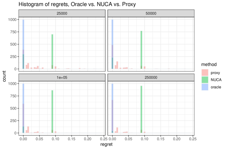
Figure 2: For each of the 4 sample sizes, we plot the regrets of the estimated optimal regime using the proxy, NUCA, and oracle methods over 1000 iterations.

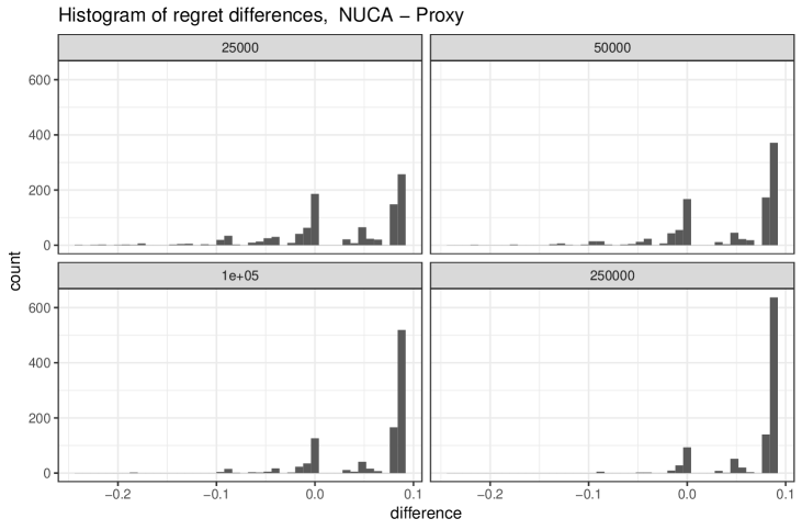
Figure 3: For each of the 4 sample sizes, we plot for each of the 1000 iterations, the difference in regret between the NUCA and proxy estimated optimal regimes. Larger difference indicates worse performance for NUCA.

We notice that the oracle method, at all sample sizes, consistently identifies the optimal regime. Meanwhile, over 1000 iterations, the proxy methods outperform NUCA in terms of the average regret and $q$-quantile regret for all but $q=90$ for sample size $25,000$, where the proxy methods exhibit more variability. The gaps widen as the sample size increases. For the first three sample sizes, the completely saturated proxy estimator performs similarly to the order 6 interaction proxy estimator, but the former has worse worst-case performance than the latter at $N=250,000$.

6 Discussion

The current literature on estimating optimal dynamic treatment regimes in the presence of unmeasured confounding is sparse. We contribute to this literature by establishing identification assuming the existence of special proxy variables and solutions to certain integral equations. We provide closed-form solutions and empirical results in the categorical case. However, estimation and inference in the continuous case can be significantly more challenging, as it potentially involves solving ill-posed integral equations and is a promising avenue for future research. It would also be interesting to develop new highly efficient and robust semiparametric estimators that exhibit better worst-case performance than the simple plug-in estimators we examined in the simulation study. Finally, examining the implications of non-unique solutions to the integral equations (Zhang et al. (2023), Bennett et al. (2023)) could be of interest.

Appendix A Proofs of Main Results

A.1 Known results

We first state some well-known results about identification in longitudinal observational studies under sequential randomization. First, recall that the joint potential outcome density is as follows:

$$f\left(Y_{2}\left(a_{1},a_{2}\right)=y_{2},Y_{1}\left(a_{1}\right)=y_{1}|y_{0}\right)$$ (6)

$$=\sum_{u_{0}}f\left(Y_{2}\left(a_{1},a_{2}\right)=y_{2},Y_{1}\left(a_{1}\right)=y_{1}|y_{0},u_{0}\right)f(u_{0}|y_{0})$$

$$=\sum_{u_{0}}f\left(Y_{2}\left(a_{1},a_{2}\right)=y_{2},Y_{1}\left(a_{1}\right)=y_{1}|y_{0},u_{0},a_{1}\right)f(u_{0}|y_{0})$$

$$=\sum_{u_{0}}f\left(Y_{2}\left(a_{1},a_{2}\right)=y_{2},Y_{1}=y_{1}|y_{0},u_{0},a_{1}\right)f(u_{0}|y_{0})$$

$$=\sum_{u_{0},u_{1}}f\left(Y_{2}\left(a_{1},a_{2}\right)=y_{2}|\overline{y}_{1},\overline{u}_{1},a_{1}\right)f\left(U_{1}=u_{1}|y_{1},y_{0}\ ,u_{0},a_{1}\right)f(y_{1}|y_{0},u_{0},a_{1})f(u_{0}|y_{0})$$

$$=\sum_{u_{0},u_{1}}f\left(Y_{2}\left(a_{1},a_{2}\right)=y_{2}|\overline{y}_{1},\overline{u}_{1},\overline{a}_{2}\right)f\left(U_{1}=u_{1}|y_{1},y_{0}\ ,u_{0},a_{1}\right)f(y_{1}|y_{0},u_{0},a_{1})f(u_{0}|y_{0})$$

$$=\sum_{u_{0},u_{1}}f\left(Y_{2}=y_{2}|\overline{y}_{1},\overline{u}_{1},\overline{a}_{2}\right)f\left(U_{1}=u_{1}|y_{1},y_{0}\ ,u_{0},a_{1}\right)f(y_{1}|y_{0},u_{0},a_{1})f(u_{0}|y_{0}).$$

The second equality is due to $\{Y_{2}(a_{1},a_{2}),Y_{1}(a_{1})\}\perp\!\!\!\perp A_{1}\mid Y_{0},U_{0}$ and the fifth is due to $Y_{2}(a_{1},a_{2})\perp\!\!\!\perp A_{2}\mid\overline{Y}_{1},\overline{U}_{1},A_{1}=a_{1}$. The third and sixth equality are by consistency. Meanwhile, the single counterfactual density is likewise identified as such:

$$f\left(Y_{1}\left(a_{1}\right)=y_{1}|y_{0}\right) =\sum_{u_{0}}f\left(Y_{1}\left(a_{1}\right)=y_{1}|y_{0},u_{0}\right)f\left(u_{0}|y_{0}\right)$$ (7)

$$=\sum_{u_{0}}f\left(Y_{1}\left(a_{1}\right)=y_{1}|a_{1},y_{0},u_{0}\right)f\left(u_{0}|y_{0}\right)$$

$$=\sum_{u_{0}}f\left(Y_{1}=y_{1}|a_{1},y_{0},u_{0}\right)f\left(u_{0}|y_{0}\right).$$

The second equality is by $Y_{1}(a_{1})\perp\!\!\!\perp A_{1}\mid Y_{0},U_{0}$ and the third is by consistency.

A.2 Proof of Theorem 1

Proof.

We first show the identification of the joint density.

$$\sum_{w_{1}}h_{21}\left(\overline{y}_{2},w_{1},\overline{a}_{2}\right)f\left(w_{1}|y_{0}\right)$$

$$= \sum_{u_{0}}\sum_{w_{1}}h_{21}\left(\overline{y}_{2},w_{1},\overline{a}_{2}\right)f\left(w_{1}|y_{0},u_{0}\right)f\left(u_{0}|y_{0}\right)$$

$$= \sum_{u_{0}}\sum_{w_{1}}h_{21}\left(\overline{y}_{2},w_{1},\overline{a}_{2}\right)f\left(w_{1}|y_{0},a_{1},u_{0}\right)f\left(u_{0}|y_{0}\right)$$

$$= \sum_{u_{0}}\sum_{\overline{w}_{2}}h_{22}\left(\overline{y}_{2},\overline{w}_{2},\overline{a}_{2}\right)f(y_{1}|y_{0},u_{0},a_{1})f\left(\overline{w}_{2}|\overline{y}_{1},a_{1},u_{0}\right)f\left(u_{0}|y_{0}\right)$$

$$= \sum_{u_{0}}\sum_{\overline{w}_{2}}\sum_{u_{1}}h_{22}\left(\overline{y}_{2},\overline{w}_{2},\overline{a}_{2}\right)f(y_{1}|y_{0},u_{0},a_{1})f\left(\overline{w}_{2}|\overline{y}_{1},a_{1},u_{0},u_{1}\right)f\left(u_{1}|\overline{y}_{1},a_{1},u_{0}\right)f\left(u_{0}|y_{0}\right)$$

$$= \sum_{u_{0}}\sum_{u_{1}}\left\{\sum_{\overline{w}_{2}}h_{22}\left(\overline{y}_{2},\overline{w}_{2},\overline{a}_{2}\right)f\left(\overline{w}_{2}|\overline{y}_{1},\overline{a}_{2},u_{0},u_{1}\right)\right\}f\left(u_{1}|\overline{y}_{1},a_{1},u_{0}\right)f\left(y_{1}|y_{0},a_{1},u_{0}\right)f\left(u_{0}|y_{0}\right)$$

$$= \sum_{u_{0}}\sum_{u_{1}}f\left(Y_{2}=y_{2}|\overline{y}_{1},\overline{u}_{1},\overline{a}_{2}\right)f\left(u_{1}|\overline{y}_{1},a_{1},u_{0}\right)f\left(y_{1}|y_{0},a_{1},u_{0}\right)f\left(u_{0}|y_{0}\right)$$

$$= f\left(Y_{2}\left(a_{1},a_{2}\right)=y_{2},Y_{1}\left(a_{1}\right)=y_{1}|y_{0}\right)$$

The first and fourth equalities follow from basic probability algebra, the second and fifth from Assumption 1 ($A_{1}\perp\!\!\!\perp W_{1}\mid U_{0},Y_{0}$ and $A_{2}\perp\!\!\!\perp\overline{W}_{2}\mid\overline{U}_{1},\overline{Y}_{1},A_{1}$), the third and sixth from Assumption 2, and the final equality is by the g-formula, restated in the previous subsection in Equation 17. ∎

A.3 Proof of Lemma 1

The conditions from Assumption 3 were assumed in Ying et al. [2023]. Using these conditions, showing that if $h_{22}$ solves its respective integral equation on the observed data (i.e. conditioned on $Z$), that it solves the respective integral equation on the latent scale (i.e. conditioned on $U$), follows the usual steps, see Ying et al. [2023]. The steps for $h_{21}$ are slightly different.

Proof.

Suppose we have a $h_{21}\left(\overline{y}_{1},w_{1},\overline{a}_{2}\right)$ that satisfies

$$\sum_{\overline{w}_{2}}h_{22}\left(\overline{y}_{2},\overline{w}_{2},\overline{a}_{2}\right)f\left(\overline{w}_{2}|\overline{y}_{1},a_{1},z_{1}\right)f(y_{1}|y_{0},\ a_{1},z_{1})=\sum_{w_{1}}h_{21}\left(\overline{y}_{2},w_{1},\overline{a}_{2}\right)f\left(w_{1}|y_{0},a_{1},z_{1}\right).$$ (8)

We can rewrite

$$f\left(\overline{w}_{2}|\overline{y}_{1},a_{1},z_{1}\right)f(y_{1}|y_{0},\ a_{1},z_{1}) =f\left(\overline{w}_{2},y_{1}|{y}_{0},a_{1},z_{1}\right)$$

$$=\sum_{u_{0}}f\left(\overline{w}_{2},y_{1}|{y}_{0},u_{0},a_{1},z_{1}\right)f(u_{0}\mid{y}_{0},a_{1},z_{1})$$

$$=\sum_{u_{0}}f\left(\overline{w}_{2},y_{1}|{y}_{0},u_{0},a_{1}\right)f(u_{0}\mid{y}_{0},a_{1},z_{1}),$$

where the last equality is by Assumption 1, namely $\{\overline{W}_{2},Y_{1}\}\perp\!\!\!\perp Z_{1}\mid A_{1},Y_{0},U_{0}$, and

$$\sum_{w_{1}}h_{21}\left(\overline{y}_{2},w_{1},\overline{a}_{2}\right)f\left(w_{1}|y_{0},a_{1},z_{1}\right) =\sum_{w_{1}}h_{21}\left(\overline{y}_{2},w_{1},\overline{a}_{2}\right)\sum_{u_{0}}f\left(w_{1}|y_{0},a_{1},u_{0},z_{1}\right)f(u_{0}\mid y_{0},a_{1},z_{1})$$

$$=\sum_{w_{1}}h_{21}\left(\overline{y}_{2},w_{1},\overline{a}_{2}\right)\sum_{u_{0}}f\left(w_{1}|y_{0},a_{1},u_{0}\right)f(u_{0}\mid y_{0},a_{1},z_{1}),$$

where the second equality is by Assumption 1, namely ${W}_{1}\perp\!\!\!\perp Z_{1}\mid A_{1},Y_{0},U_{0}$. Then we can write equation (6) as

$$\sum_{\overline{w}_{2}}h_{22}\left(\overline{y}_{2},\overline{w}_{2},\overline{a}_{2}\right) \sum_{u_{0}}f\left(\overline{w}_{2},y_{1}|{y}_{0},u_{0},a_{1}\right)f(u_{0}\mid{y}_{0},a_{1},z_{1})$$ (9)

$$=\sum_{w_{1}}h_{21}\left(\overline{y}_{2},w_{1},\overline{a}_{2}\right)\sum_{u_{0}}f\left(w_{1}|y_{0},a_{1},u_{0}\right)f(u_{0}\mid y_{0},a_{1},z_{1})$$

Fixing $\overline{y}_{2},\overline{a}_{2}$ and interchanging the order of the integrals, we have

$$\sum_{u_{0}}\sum_{\overline{w}_{2}}h_{22}\left(\overline{y}_{2},\overline{w}_{2},\overline{a}_{2}\right) f\left(\overline{w}_{2},y_{1}|{y}_{0},u_{0},a_{1}\right)f(u_{0}\mid{y}_{0},a_{1},z_{1})$$ (10)

$$=\sum_{u_{0}}\sum_{w_{1}}h_{21}\left(\overline{y}_{2},w_{1},\overline{a}_{2}\right)f\left(w_{1}|y_{0},a_{1},u_{0}\right)f(u_{0}\mid y_{0},a_{1},z_{1})$$

Then by the second completeness condition in Assumption 3,

$$\sum_{\overline{w}_{2}}h_{22}\left(\overline{y}_{2},\overline{w}_{2},\overline{a}_{2}\right)f\left(\overline{w}_{2},y_{1}|{y}_{0},u_{0},a_{1}\right)=\sum_{w_{1}}h_{21}\left(\overline{y}_{2},w_{1},\overline{a}_{2}\right)f\left(w_{1}|y_{0},a_{1},u_{0}\right).$$

We show the steps for the $h_{22}$ function for sake of completeness. Suppose there is a $h_{22}\left(\overline{y}_{2},\overline{w}_{2},\overline{a}_{2}\right)$ that solves

$$f\left(Y_{2}=y_{2}|\overline{y}_{1},\overline{z}_{2},\overline{a}_{2}\right)=\sum_{\overline{w}_{2}}h_{22}\left(\overline{y}_{2},\overline{w}_{2},\overline{a}_{2}\right)f\left(\overline{w}_{2}|\overline{y}_{1},\overline{a}_{2},\overline{z}_{2}\right).$$

From Assumption 1, $Y_{2}\perp\!\!\!\perp\overline{Z}_{2}\mid\overline{Y}_{1},\overline{U}_{1},\overline{A}_{2}$ and $\overline{W}_{2}\perp\!\!\!\perp\overline{Z}_{2}\mid\overline{Y}_{1},\overline{U}_{1},\overline{A}_{2}$ hold. Thus,

$$f\left(Y_{2}=y_{2}|\overline{y}_{1},\overline{z}_{2},\overline{a}_{2}\right) =\sum_{\overline{u}_{1}}f\left(Y_{2}=y_{2}|\overline{y}_{1},\overline{z}_{2},\overline{a}_{2},\overline{u}_{1}\right)f(\overline{u}_{1}\mid\overline{y}_{1},\overline{z}_{2},\overline{a}_{2})$$

$$=\sum_{\overline{u}_{1}}f\left(Y_{2}=y_{2}|\overline{y}_{1},\overline{a}_{2},\overline{u}_{1}\right)f(\overline{u}_{1}\mid\overline{y}_{1},\overline{z}_{2},\overline{a}_{2}),$$

$$\sum_{\overline{w}_{2}}h_{22}\left(\overline{y}_{2},\overline{w}_{2},\overline{a}_{2}\right)f\left(\overline{w}_{2}|\overline{y}_{1},\overline{a}_{2},\overline{z}_{2}\right) =\sum_{\overline{w}_{2}}\sum_{\overline{u}_{1}}h_{22}\left(\overline{y}_{2},\overline{w}_{2},\overline{a}_{2}\right)f\left(\overline{w}_{2}|\overline{y}_{1},\overline{a}_{2},\overline{z}_{2},\overline{u}_{1}\right)f(\overline{u}_{1}\mid\overline{y}_{1},\overline{z}_{2},\overline{a}_{2})$$

$$=\sum_{\overline{u}_{1}}\sum_{\overline{w}_{2}}h_{22}\left(\overline{y}_{2},\overline{w}_{2},\overline{a}_{2}\right)f\left(\overline{w}_{2}|\overline{y}_{1},\overline{a}_{2},\overline{u}_{1}\right)f(\overline{u}_{1}\mid\overline{y}_{1},\overline{z}_{2},\overline{a}_{2}).$$

Applying the first completeness condition from Assumption 3 implies that

$$f\left(Y_{2}=y_{2}|\overline{y}_{1},\overline{a}_{2},\overline{u}_{1}\right)=\sum_{\overline{w}_{2}}h_{22}\left(\overline{y}_{2},\overline{w}_{2},\overline{a}_{2}\right)f\left(\overline{w}_{2}|\overline{y}_{1},\overline{a}_{2},\overline{u}_{1}\right).$$

∎

A.4 Proof of Proposition 1

Proof.

Recall that

$$f\left(Y_{2}=y_{2}|\overline{y}_{1},\overline{u}_{1},\overline{a}_{2}\right)=\sum_{\overline{w}_{2}}h_{22}\left(\overline{y}_{2},\overline{w}_{2},\overline{a}_{2}\right)f\left(\overline{w}_{2}|\overline{y}_{1},\overline{a}_{2},\overline{u}_{1}\right)$$

By causal consistency and Assumption 1, the left hand side can be rewritten as $f\left(Y_{2}(a_{1},a_{2})=y_{2}|\overline{y}_{1},\overline{u}_{1},a_{1}\right)$ and the right hand side as $\sum_{\overline{w}_{2}}h_{22}\left(\overline{y}_{2},\overline{w}_{2},\overline{a}_{2}\right)f\left(\overline{w}_{2}|\overline{y}_{1},{a}_{1},\overline{u}_{1}\right)$. Thus, we get

$$\sum_{u_{1}}f\left(Y_{2}(a_{1},a_{2})=y_{2}|\overline{y}_{1},\overline{u}_{1},a_{1}\right)f(u_{1}\mid\overline{y}_{1},{u}_{0},a_{1})=\sum_{u_{1}}\sum_{\overline{w}_{2}}h_{22}\left(\overline{y}_{2},\overline{w}_{2},\overline{a}_{2}\right)f\left(\overline{w}_{2}|\overline{y}_{1},{a}_{1},\overline{u}_{1}\right)f(u_{1}\mid\overline{y}_{1},{u}_{0},a_{1})$$

$$\sum_{u_{1}}f\left(Y_{2}(a_{1},a_{2})=y_{2},u_{1}|\overline{y}_{1},{u}_{0},a_{1}\right)=\sum_{\overline{w}_{2}}\sum_{u_{1}}h_{22}\left(\overline{y}_{2},\overline{w}_{2},\overline{a}_{2}\right)f\left(\overline{w}_{2},u_{1}|\overline{y}_{1},{u}_{0},a_{1}\right)$$

$$f\left(Y_{2}(a_{1},a_{2})=y_{2}|\overline{y}_{1},{u}_{0},a_{1}\right)=\sum_{\overline{w}_{2}}h_{22}\left(\overline{y}_{2},\overline{w}_{2},\overline{a}_{2}\right)f\left(\overline{w}_{2}|\overline{y}_{1},{u}_{0},a_{1}\right)$$

$$\implies\sum_{y_{2}}\sum_{\overline{w}_{2}}h_{22}\left(\overline{y}_{2},\overline{w}_{2},\overline{a}_{2}\right)f\left(\overline{w}_{2}|\overline{y}_{1},{u}_{0},a_{1}\right)=1$$

Plugging this into the integral equation involving $h_{21}$, we get

$$\sum_{y_{2}}\sum_{w_{1}}h_{21}\left(\overline{y}_{2},w_{1},\overline{a}_{2}\right)f\left(w_{1}|y_{0},a_{1},u_{0}\right) =\sum_{y_{2}}\sum_{\overline{w}_{2}}h_{22}\left(\overline{y}_{2},\overline{w}_{2},\overline{a}_{2}\right)f(y_{1}|y_{0},u_{0},a_{1})f\left(\overline{w}_{2}|\overline{y}_{1},a_{1},u_{0}\right)$$

$$=f(y_{1}|y_{0},u_{0},a_{1})\sum_{y_{2}}\sum_{\overline{w}_{2}}h_{22}\left(\overline{y}_{2},\overline{w}_{2},\overline{a}_{2}\right)f\left(\overline{w}_{2}|\overline{y}_{1},a_{1},u_{0}\right)$$

$$=f(y_{1}|y_{0},u_{0},a_{1})$$

After interchanging summation of $y_{2}$ and $w_{1}$, it immediately follows that $\sum_{y_{2}}h_{21}(\overline{y}_{2},w_{1},\overline{a}_{2})$ solves Equation 5. ∎

A.5 Proof of Proposition 2

Proof.

See the proof of Proposition 3 in Section D of the supplement. ∎

Appendix B Existence and uniqueness of bridge functions

B.1 Existence

Similar to Ying et al. [2023] and Miao et al. [2018], we consider the singular value decomposition (Carrasco et al. [2007], Theorem 2.41) of compact operators to characterize conditions for existence of a solutions to the integral equations from Equation 4. Let $L_{2}\{F(t)\}$ denote the space of all square integrable functions of t with respect to a cumulative distribution function $F(t)$, which is a Hilbert space with inner product $\langle g,h\rangle=\int g(t)h(t)dF(t)$. Define $T_{\overline{a}_{k},\overline{y}_{k-1}}$ as the conditional expectation operator, mapping $L_{2}\{F(\overline{w}_{k}\mid\overline{a}_{k},\overline{y}_{k-1})\}\to L_{2}\{F(\overline{z}_{k}\mid\overline{a}_{k},\overline{y}_{k-1})\}$ and $T_{\overline{a}_{k},\overline{y}_{k-1}}h=E[h(\overline{W}_{k})\mid\overline{z}_{k},\overline{a}_{k},\overline{y}_{k-1}]$. Let $(\lambda_{\overline{a}_{k},\overline{y}_{k-1},l},\psi_{\overline{a}_{k},\overline{y}_{k-1},l},\phi_{\overline{a}_{k},\overline{y}_{k-1},l})_{l=1}^{\infty}$ denote a singular value decomposition for $T_{\overline{a}_{k},\overline{y}_{k-1}}$. We assume the following:

Assumption 5 (Regularity conditions for existence).

1. $\sum_{k=1}^{2}\int\int f(\overline{w}_{k}\mid\overline{z}_{k},\overline{a}_{k},\overline{y}_{k-1})f(\overline{z}_{k}\mid\overline{w}_{k},\overline{a}_{k},\overline{y}_{k-1})d\overline{w}_{k}d\overline{z}_{k}<\infty$.

2. For fixed $y_{0},y_{1},y_{2},a_{1},a_{2}$,

   $$\int f^{2}(y_{2}\mid\overline{z}_{2},\overline{a}_{2},\overline{y}_{1})f(\overline{z}_{2}\mid\overline{a}_{2},\overline{y}_{1})d\overline{z}_{2}<\infty,$$

   $$\int\left(\sum_{\overline{w}_{2}}h_{22}\left(\overline{y}_{2},\overline{w}_{2},\overline{a}_{2}\right)f\left(\overline{w}_{2}|\overline{y}_{1},a_{1},z_{1}\right)f(y_{1}|y_{0},a_{1},z_{1})\right)^{2}f(z_{1}\mid a_{1},y_{0})dz_{1}<\infty.$$

3. For fixed $y_{0},y_{1},y_{2},a_{1},a_{2}$,

   $$\sum_{l=1}^{\infty}\lambda^{-2}_{\overline{a}_{2},\overline{y}_{1},l}\langle f(y_{2}\mid\overline{z}_{2},\overline{a}_{2},\overline{y}_{1}),\phi_{\overline{a}_{2},\overline{y}_{1},l}\rangle^{2}<\infty,$$

   $$\sum_{l=1}^{\infty}\lambda^{-2}_{a_{1},y_{0},l}\left\langle\sum_{\overline{w}_{2}}h_{22}\left(\overline{y}_{2},\overline{w}_{2},\overline{a}_{2}\right)f\left(\overline{w}_{2}|\overline{y}_{1},a_{1},z_{1}\right)f(y_{1}|y_{0},a_{1},z_{1}),\phi_{a_{1},y_{0},l}\right\rangle^{2}<\infty.$$

4. For any square integrable $g_{1}$, we have that

   $${E}[g_{1}(\overline{Z}_{2})\mid\overline{y}_{1},\overline{w}_{2},\overline{a}_{2}]=0\text{ implies }g_{1}(\overline{Z}_{2})=0.$$

   In addition, for any square integrable $g_{0}$, we have that

   $${E}[g_{0}(Z_{1})\mid{y}_{0},w_{1},{a}_{1}]=0\text{ implies }g_{0}(Z_{1})=0.$$

Lemma 2.

Under Assumption 5, there exist $h_{22}$ and $h_{21}$ that satisfy the respective integral equations from Equation 4 from Lemma 1.

Proof.

The proof follows straightforwardly from Picard’s theorem (Kress [1999]) and Lemma 2 from Miao et al. [2018]. ∎

B.2 Uniqueness

In this subsection, we introduce an additional completeness assumption that guarantees that solutions to the observed integral equations are unique.

Assumption 6.

For any square integrable $g_{1}$, we have that

$${E}[g_{1}(\overline{W}_{2})\mid\overline{y}_{1},\overline{z}_{2},\overline{a}_{2}]=0\text{ implies }g_{1}(\overline{W}_{2})=0.$$

In addition, for any square integrable $g_{0}$, we have that

$${E}[g_{0}(W_{1})\mid{y}_{0},z_{1},{a}_{1}]=0\text{ implies }g_{0}(W_{1})=0.$$

Lemma 3.

Suppose there exist $h_{22}$ and $h_{21}$ that solve the intergal equations from Lemma 1. Then under Assumption 6, $h_{22}$ and $h_{21}$ are unique.

Proof.

First, suppose that $h_{22}$ and $h^{\prime}_{22}$ both solve the integral equation. Then

$$\sum_{\overline{w}_{2}}h_{22}\left(\overline{y}_{2},\overline{w}_{2},\overline{a}_{2}\right)f\left(\overline{w}_{2}|\overline{y}_{1},\overline{a}_{2},\overline{z}_{2}\right)=\sum_{\overline{w}_{2}}h^{\prime}_{22}\left(\overline{y}_{2},\overline{w}_{2},\overline{a}_{2}\right)f\left(\overline{w}_{2}|\overline{y}_{1},\overline{a}_{2},\overline{z}_{2}\right).$$

Subtracting, we get

$${E}[h_{22}\left(\overline{y}_{2},\overline{W}_{2},\overline{a}_{2}\right)-h^{\prime}_{22}\left(\overline{y}_{2},\overline{W}_{2},\overline{a}_{2}\right)|\overline{y}_{1},\overline{a}_{2},\overline{z}_{2}]=0\implies h_{22}\left(\overline{y}_{2},\overline{W}_{2},\overline{a}_{2}\right)-h^{\prime}_{22}\left(\overline{y}_{2},\overline{W}_{2},\overline{a}_{2}\right)=0.$$

Next, suppose that $h_{21}$ and $h^{\prime}_{21}$ both solve the corresponding integral equation. Then by the uniqueness of $h_{22}$, we get

$$\sum_{w_{1}}h_{21}\left(\overline{y}_{2},w_{1},\overline{a}_{2}\right)f\left(w_{1}|y_{0},a_{1},z_{1}\right)=\sum_{w_{1}}h^{\prime}_{21}\left(\overline{y}_{2},w_{1},\overline{a}_{2}\right)f\left(w_{1}|y_{0},a_{1},z_{1}\right).$$

Subtracting, we get

$${E}[h_{21}\left(\overline{y}_{2},W_{1},\overline{a}_{2}\right)-h^{\prime}_{21}\left(\overline{y}_{2},W_{1},\overline{a}_{2}\right)|y_{0},a_{1},z_{1}]=0\implies h_{21}\left(\overline{y}_{2},W_{1},\overline{a}_{2}\right)-h^{\prime}_{21}\left(\overline{y}_{2},W_{1},\overline{a}_{2}\right)=0.$$

∎

Appendix C General number of timepoints

In this section, we demonstrate that the results from previous sections can be extended the case where the number of time periods $K>2$. The data has the following form:

$$(U_{0},\ldots,U_{K-1},Y_{0},\ldots,Y_{K},A_{1},\ldots,A_{K},Z_{1},\ldots,Z_{K},W_{1},\ldots,W_{K}),$$

where the $U$ variables are unobserved. We first introduce the general versions of the latent randomization, bridge function, and completeness assumptions.

Assumption 7 (Sequential Proximal Latent Randomization - General Case).

$$\left\{{Y}_{1}\left(a_{1}\right),\ldots,Y_{k}\left(a_{1},\ldots a_{k}\right),\overline{W}_{k}\right\}\perp\!\!\!\perp A_{k},\overline{Z}_{k}|\left(\overline{U}_{k-1},\overline{Y}_{k-1},\overline{A}_{k-1}=\overline{a}_{k-1}\right)\text{ for }k=1,\ldots,K.$$

$$\{\overline{W}_{k+1},Y_{k}\}\perp\!\!\!\perp\overline{Z}_{k}\mid\overline{A}_{k},\overline{U}_{k-1},\overline{Y}_{k-1}\text{ for }k=1,\ldots,K-1.$$

Assumption 8 (Bridge Functions - General Case).

There exist functions $h_{KK}(\bar{y}_{K},\bar{w}_{K},\bar{a}_{K}),\ldots,h_{K1}(\bar{y}_{K},\bar{w}_{1},\bar{a}_{K})$ that satisfy

$$f(Y_{K}=y_{K}\mid\bar{y}_{K-1},\bar{u}_{K-1},\bar{a}_{K})=\sum_{\bar{w}_{K}}h_{KK}(\bar{y}_{K},\bar{w}_{K},\bar{a}_{K})f(\bar{w}_{K}\mid\bar{y}_{K-1},\bar{u}_{K-1},\bar{a}_{K}),$$

and for $k=1,\ldots,K-1$,

$$\sum_{\bar{w}_{k+1}}h_{K,k+1}(\bar{y}_{K},\bar{w}_{k+1},\bar{a}_{K})f(\bar{w}_{k+1},y_{k}\mid\bar{y}_{k-1},\bar{u}_{k-1},\bar{a}_{k})=\sum_{\bar{w}_{k}}h_{Kk}(\bar{y}_{K},\bar{w}_{k},\bar{a}_{K})f(\bar{w}_{k}\mid\bar{y}_{k-1},\bar{u}_{k-1},\bar{a}_{k}).$$

Assumption 9 (Completeness - General Case).

For each $k=1,\ldots,K$ and any square integrable $g=g(\overline{U}_{k-1})$,

$$E[g(\overline{U}_{k-1}\mid\overline{y}_{k-1},\overline{z}_{k},\overline{a}_{k}]\text{ implies }g(\overline{U}_{k-1})=0.$$

Lemma 4.

Under Assumptions 7 and 8, the following equation holds:

$$\sum_{\bar{w}_{k}} h_{Kk}(\bar{y}_{K},\bar{w}_{k},\bar{a}_{K})f(\bar{w}_{k}\mid\bar{y}_{k-1},\bar{u}_{k-1},\bar{a}_{k})$$

$$=\sum_{u_{k}}\sum_{\bar{w}_{k+1}}h_{K,k+1}(\bar{y}_{K},\bar{w}_{k+1},\bar{a}_{K})f(\bar{w}_{k+1}\mid\bar{y}_{k},\bar{u}_{k},\bar{a}_{k+1})f(u_{k}\mid\bar{u}_{k-1},\bar{y}_{k},\bar{a}_{k})f(y_{k}\mid\bar{u}_{k-1},\bar{y}_{k-1},\bar{a}_{k}).$$

Proof.

$$\sum_{\bar{w}_{k}} h_{Kk}(\bar{y}_{K},\bar{w}_{k},\bar{a}_{K})f(\bar{w}_{k}\mid\bar{y}_{k-1},\bar{u}_{k-1},\bar{a}_{k})$$

$$=\sum_{\bar{w}_{k+1}}h_{K,k+1}(\bar{y}_{K},\bar{w}_{k+1},\bar{a}_{K})f(\bar{w}_{k+1},y_{k}\mid\bar{y}_{k-1},\bar{u}_{k-1},\bar{a}_{k})$$

$$=\sum_{\bar{w}_{k+1}}h_{K,k+1}(\bar{y}_{K},\bar{w}_{k+1},\bar{a}_{K})f(\bar{w}_{k+1}\mid\bar{y}_{k},\bar{u}_{k-1},\bar{a}_{k})f(y_{k}\mid\bar{y}_{k-1},\bar{u}_{k-1},\bar{a}_{k})$$

$$=\sum_{\bar{w}_{k+1}}\sum_{u_{k}}h_{K,k+1}(\bar{y}_{K},\bar{w}_{k+1},\bar{a}_{K})f(\bar{w}_{k+1},u_{k}\mid\bar{y}_{k},\bar{u}_{k-1},\bar{a}_{k})f(y_{k}\mid\bar{y}_{k-1},\bar{u}_{k-1},\bar{a}_{k})$$

$$=\sum_{\bar{w}_{k+1}}\sum_{u_{k}}h_{K,k+1}(\bar{y}_{K},\bar{w}_{k+1},\bar{a}_{K})f(\bar{w}_{k+1}\mid\bar{y}_{k},\bar{u}_{k},\bar{a}_{k})f(u_{k}\mid\bar{y}_{k},\bar{u}_{k-1},\bar{a}_{k})f(y_{k}\mid\bar{y}_{k-1},\bar{u}_{k-1},\bar{a}_{k})$$

$$=\sum_{u_{k}}\sum_{\bar{w}_{k+1}}h_{K,k+1}(\bar{y}_{K},\bar{w}_{k+1},\bar{a}_{K})f(\bar{w}_{k+1}\mid\bar{y}_{k},\bar{u}_{k},\bar{a}_{k+1})f(u_{k}\mid\bar{u}_{k-1},\bar{y}_{k},\bar{a}_{k})f(y_{k}\mid\bar{u}_{k-1},\bar{y}_{k-1},\bar{a}_{k}).$$

By assumption 8, the first equality holds. The second, third, and fourth equality follow from standard probability algebra, and the last follows from $A_{k+1}\perp\!\!\!\perp\bar{W}_{k+1}\mid\bar{Y}_{k},\bar{U}_{k},\overline{A}_{k}=\overline{a}_{k}$. ∎

Theorem 2.

Under Assumptions 7 and 8,

$$f(Y_{K}(a_{1},\ldots,a_{K})=y_{K},\ldots,Y_{1}(a_{1})=y_{1}\mid y_{0})=\sum_{w_{1}}h_{K1}(\bar{y}_{K},w_{1},\bar{a}_{K})f(w_{1}\mid y_{0}).$$

Proof.

By Lemma 4,

$$\sum_{w_{1}} h_{K1}(\bar{y}_{K},w_{1},\bar{a}_{K})f(w_{1}\mid y_{0})=\sum_{u_{0}}\sum_{w_{1}}h_{K1}(\bar{y}_{K},w_{1},\bar{a}_{K})f(w_{1}\mid y_{0},u_{0},a_{1})f(u_{0}\mid y_{0})$$

$$=\sum_{u_{0}}\sum_{u_{1}}\sum_{\bar{w}_{2}}h_{K2}(\bar{y}_{K},\bar{w}_{2},\bar{a}_{K})f(\bar{w}_{2}\mid\bar{y}_{1},\bar{u}_{1},\bar{a}_{2})f(u_{1}\mid u_{0},\bar{y}_{1},a_{1})f(y_{1}\mid u_{0},y_{0},a_{1})f(u_{0}\mid y_{0})$$

$$\vdots$$

$$=\sum_{\bar{u}_{K-1}}\sum_{\bar{w}_{K}}h_{KK}(\bar{y}_{K},\bar{w}_{K},\bar{a}_{K})f(\bar{w}_{K}\mid\bar{y}_{K-1},\bar{u}_{K-1},\bar{a}_{K})\left\{\prod_{j=1}^{K-1}f(u_{j}\mid\bar{u}_{j-1},\bar{y}_{j},\bar{a}_{j})f(y_{j}\mid\bar{u}_{j-1},\bar{y}_{-1},\bar{a}_{j})\right\}f(u_{0}\mid y_{0})$$

$$=\sum_{\bar{u}_{K-1}}f(Y_{K}=y_{K}\mid\bar{y}_{K-1},\bar{u}_{K-1},\bar{a}_{K})\left\{\prod_{j=1}^{K-1}f(u_{j}\mid\bar{u}_{j-1},\bar{y}_{j},\bar{a}_{j})f(y_{j}\mid\bar{u}_{j-1},\bar{y}_{-1},\bar{a}_{j})\right\}f(u_{0}\mid y_{0})$$

$$=f(Y_{K}(a_{1},\ldots,a_{K})=y_{K},\ldots,Y_{1}(a_{1})=y_{1}\mid y_{0}).$$

The first equality follows by basic probability, the inner equalities all follow from Lemma 4, the second to last equality follows from Assumption 8, and the last follows by the usual g-formula, since we have sequential exchangeability given the $Y$ and $U$ variables from Assumption 7. ∎

In the following lemma, similar to the $K=2$ case, we link the latent bridge functions to observable bridge functions.

Lemma 5.

Suppose that there exist functions $h_{KK},\ldots,h_{K1}$ that satisfy

$$f(Y_{K}=y_{K}\mid\bar{y}_{K-1},\bar{z}_{K},\bar{a}_{K})=\sum_{\bar{w}_{K}}h_{KK}(\bar{y}_{K},\bar{w}_{K},\bar{a}_{K})f(\bar{w}_{K}\mid\bar{y}_{K-1},\bar{z}_{K},\bar{a}_{K}),$$

and for $k=1,\ldots,K-1$,

$$\sum_{\bar{w}_{k+1}}h_{K,k+1}(\bar{y}_{K},\bar{w}_{k+1},\bar{a}_{K})f(\bar{w}_{k+1},y_{k}\mid\bar{y}_{k-1},\bar{z}_{k},\bar{a}_{k})=\sum_{\bar{w}_{k}}h_{Kk}(\bar{y}_{K},\bar{w}_{k},\bar{a}_{K})f(\bar{w}_{k}\mid\bar{y}_{k-1},\bar{z}_{k},\bar{a}_{k}).$$

If Assumption 7 and 9 hold, then $h_{KK},\ldots,h_{K1}$ solve the respective integral equations from Assumption 8 as well.

Proof.

Fix a $k$. Suppose that

$$\sum_{\bar{w}_{k+1}}h_{K,k+1}(\bar{y}_{K},\bar{w}_{k+1},\bar{a}_{K})f(\bar{w}_{k+1},y_{k}\mid\bar{y}_{k-1},\bar{z}_{k},\bar{a}_{k})=\sum_{\bar{w}_{k}}h_{Kk}(\bar{y}_{K},\bar{w}_{k},\bar{a}_{K})f(\bar{w}_{k}\mid\bar{y}_{k-1},\bar{z}_{k},\bar{a}_{k}).$$

We can simplify using the fact that $\{\overline{W}_{k+1},Y_{k}\}\perp\!\!\!\perp\overline{Z}_{k}\mid\overline{Y}_{k-1},\overline{A}_{k},\overline{U}_{k-1}$ and $\overline{W}_{k}\perp\!\!\!\perp\overline{Z}_{k}\mid\overline{Y}_{k-1},\overline{A}_{k},\overline{U}_{k-1}$ from Assumption 7:

$$f(\bar{w}_{k+1},y_{k}\mid\bar{y}_{k-1},\bar{z}_{k},\bar{a}_{k}) =\sum_{\overline{u}_{k-1}}f(\bar{w}_{k+1},y_{k}\mid\bar{y}_{k-1},\bar{z}_{k},\bar{a}_{k},\overline{u}_{k-1})f(\overline{u}_{k-1}\mid\bar{y}_{k-1},\bar{z}_{k},\bar{a}_{k})$$

$$=\sum_{\overline{u}_{k-1}}f(\bar{w}_{k+1},y_{k}\mid\bar{y}_{k-1},\bar{a}_{k},\overline{u}_{k-1})f(\overline{u}_{k-1}\mid\bar{y}_{k-1},\bar{z}_{k},\bar{a}_{k}),$$

$$f(\bar{w}_{k}\mid\bar{y}_{k-1},\bar{z}_{k},\bar{a}_{k}) =\sum_{\overline{u}_{k-1}}f(\bar{w}_{k}\mid\bar{y}_{k-1},\bar{z}_{k},\bar{a}_{k},\overline{u}_{k-1})f(\overline{u}_{k-1}\mid\bar{y}_{k-1},\bar{z}_{k},\bar{a}_{k})$$

$$=\sum_{\overline{u}_{k-1}}f(\bar{w}_{k}\mid\bar{y}_{k-1},\bar{z}_{k},\overline{u}_{k-1})f(\overline{u}_{k-1}\mid\bar{y}_{k-1},\bar{z}_{k},\bar{a}_{k}).$$

Plugging these equations back into the previous display and changing the order of summation, we get

$$\sum_{\overline{u}_{k-1}}\sum_{\bar{w}_{k+1}} h_{K,k+1}(\bar{y}_{K},\bar{w}_{k+1},\bar{a}_{K})f(\bar{w}_{k+1},y_{k}\mid\bar{y}_{k-1},\bar{a}_{k},\overline{u}_{k-1})f(\overline{u}_{k-1}\mid\bar{y}_{k-1},\bar{z}_{k},\bar{a}_{k})$$

$$=\sum_{\overline{u}_{k-1}}\sum_{\bar{w}_{k}}h_{Kk}(\bar{y}_{K},\bar{w}_{k},\bar{a}_{K})f(\bar{w}_{k}\mid\bar{y}_{k-1},\bar{z}_{k},\overline{u}_{k-1})f(\overline{u}_{k-1}\mid\bar{y}_{k-1},\bar{z}_{k},\bar{a}_{k}).$$

By the completeness condition from Assumption 9, we get that

$$\sum_{\bar{w}_{k+1}}h_{K,k+1}(\bar{y}_{K},\bar{w}_{k+1},\bar{a}_{K})f(\bar{w}_{k+1},y_{k}\mid\bar{y}_{k-1},\bar{a}_{k},\overline{u}_{k-1})=\sum_{\bar{w}_{k}}h_{Kk}(\bar{y}_{K},\bar{w}_{k},\bar{a}_{K})f(\bar{w}_{k}\mid\bar{y}_{k-1},\bar{z}_{k},\overline{u}_{k-1}),$$

as desired. Next, suppose that

$$f(Y_{K}=y_{K}\mid\bar{y}_{K-1},\bar{z}_{K},\bar{a}_{K})=\sum_{\bar{w}_{K}}h_{KK}(\bar{y}_{K},\bar{w}_{K},\bar{a}_{K})f(\bar{w}_{K}\mid\bar{y}_{K-1},\bar{z}_{K},\bar{a}_{K}).$$

Using the fact that $Y_{K}\perp\!\!\!\perp\overline{Z}_{K}\mid\bar{Y}_{K-1},\bar{A}_{K},\overline{U}_{K-1}$ and $\overline{W}_{K}\perp\!\!\!\perp\overline{Z}_{K}\mid\bar{Y}_{K-1},\bar{A}_{K},\overline{U}_{K-1}$ from Assumption 7,

$$f(Y_{K}=y_{K}\mid\bar{y}_{K-1},\bar{z}_{K},\bar{a}_{K}) =\sum_{\overline{u}_{K-1}}f(Y_{K}=y_{K}\mid\bar{y}_{K-1},\bar{z}_{K},\bar{a}_{K},\overline{u}_{K-1})f(\overline{u}_{K-1}\mid\bar{y}_{K-1},\bar{z}_{K},\bar{a}_{K})$$

$$=\sum_{\overline{u}_{K-1}}f(Y_{K}=y_{K}\mid\bar{y}_{K-1},\bar{a}_{K},\overline{u}_{K-1})f(\overline{u}_{K-1}\mid\bar{y}_{K-1},\bar{z}_{K},\bar{a}_{K}),$$

$$f(\bar{w}_{K}\mid\bar{y}_{K-1},\bar{z}_{K},\bar{a}_{K}) =\sum_{\overline{u}_{K-1}}f(\bar{w}_{K}\mid\bar{y}_{K-1},\bar{z}_{K},\bar{a}_{K},\overline{u}_{K-1})f(\overline{u}_{K-1}\mid\bar{y}_{K-1},\bar{z}_{K},\bar{a}_{K})$$

$$=\sum_{\overline{u}_{K-1}}f(\bar{w}_{K}\mid\bar{y}_{K-1},\bar{a}_{K},\overline{u}_{K-1})f(\overline{u}_{K-1}\mid\bar{y}_{K-1},\bar{z}_{K},\bar{a}_{K}).$$

Plugging these equations back into the previous display and changing the order of summation, we get

$$\sum_{\overline{u}_{K-1}} f(Y_{K}=y_{K}\mid\bar{y}_{K-1},\bar{a}_{K},\overline{u}_{K-1})f(\overline{u}_{K-1}\mid\bar{y}_{K-1},\bar{z}_{K},\bar{a}_{K})$$

$$=\sum_{\overline{u}_{K-1}}\sum_{\bar{w}_{K}}h_{KK}(\bar{y}_{K},\bar{w}_{K},\bar{a}_{K})f(\bar{w}_{K}\mid\bar{y}_{K-1},\bar{a}_{K},\overline{u}_{K-1})f(\overline{u}_{K-1}\mid\bar{y}_{K-1},\bar{z}_{K},\bar{a}_{K}).$$

Finally, the completeness condition from Assumption 9 implies that $f(Y_{K}=y_{K}\mid\bar{y}_{K-1},\bar{a}_{K},\overline{u}_{K-1})=\sum_{\bar{w}_{K}}h_{KK}(\bar{y}_{K},\bar{w}_{K},\bar{a}_{K})f(\bar{w}_{K}\mid\bar{y}_{K-1},\bar{a}_{K},\overline{u}_{K-1})$, completing the proof. ∎

Appendix D Over-identified Case

In this section, we examine the setting where $\min(|W_{t}|,|Z_{t}|)\geq|U_{t-1}|$ for $t=1,2$. We require a rank condition on certain matrices.

Assumption 10.

For all $(\overline{y}_{1},\overline{a}_{2})$, the matrices $P(\overline{W}_{2}\mid\overline{U}_{1},\overline{y}_{1},\overline{a}_{2})$ and $P(\overline{U}_{1}\mid\overline{Z}_{2},\overline{y}_{1},\overline{a}_{2})$ have rank $|\overline{U}_{1}|$. In addition, for all $({y}_{0},{a}_{1})$, $P({W}_{1}\mid{U}_{0},{y}_{0},{a}_{1})$ and $P({U}_{1}\mid{Z}_{1},{y}_{0},{a}_{1})$ have rank $|U_{0}|$.

Proposition 3.

Let $\infty>\min(|W_{t}|,|Z_{t}|)\geq|U_{t-1}|$ for $t=1,2$. Also, suppose Assumptions 1 and 10 hold. Then there exist solutions $h_{22}$, $h_{21}$, and $h_{11}$ solving the respective integral equations from Assumption 2 and Equation 5. In the special case where $|W_{t}|=|Z_{t}|=|U_{t-1}|$ for $t=1,2$, the conclusion of Proposition 2 holds.

Proof.

Our proof resembles the proof of Lemma 1 from Shi et al. [2020a]. Starting from the last time step, we know that $\overline{W}_{2}\perp\!\!\!\perp A_{2},\overline{Z}_{2}\mid\overline{U}_{1},\overline{Y}_{1},A_{1}=a_{1}$ and $\overline{Y}_{2}(a_{1},a_{2})\perp\!\!\!\perp A_{2},\overline{Z}_{2}\mid\overline{U}_{1},\overline{Y}_{1},A_{1}=a_{1}$, so

$$P(\overline{W}_{2}\mid\overline{Z}_{2},\overline{y}_{1},\overline{a}_{2}) =P(\overline{W}_{2}\mid\overline{U}_{1},\overline{y}_{1},{a}_{1})P(\overline{U}_{1}\mid\overline{Z}_{2},\overline{y}_{1},\overline{a}_{2})$$ (11)

$$P(y_{2}\mid\overline{Z}_{2},\overline{y}_{1},\overline{a}_{2}) =P(y_{2}\mid\overline{U}_{1},\overline{y}_{1},\overline{a}_{2})P(\overline{U}_{1}\mid\overline{Z}_{2},\overline{y}_{1},\overline{a}_{2})$$

Recall that by Assumption 10, $P(\overline{W}_{2}\mid\overline{U}_{1},\overline{y}_{1},{a}_{1})$ and $P(\overline{U}_{1}\mid\overline{Z}_{2},\overline{y}_{1},\overline{a}_{2})$ have rank $|\overline{U}_{1}|$, so they have left and right inverses, respectively. Moreover, the left and right inverses equal the Moore-Penrose pseudoinverses. We denote the Moore-Penrose pseudoinverse of a matrix $A$ by $A^{\dagger}$. We obtain

$$P(\overline{U}_{1}\mid\overline{Z}_{2},\overline{y}_{1},\overline{a}_{2}) =P(\overline{W}_{2}\mid\overline{U}_{1},\overline{y}_{1},{a}_{1})^{\dagger}P(\overline{W}_{2}\mid\overline{Z}_{2},\overline{y}_{1},\overline{a}_{2}),$$

$$P(y_{2}\mid\overline{Z}_{2},\overline{y}_{1},\overline{a}_{2}) =P(y_{2}\mid\overline{U}_{1},\overline{y}_{1},\overline{a}_{2})P(\overline{W}_{2}\mid\overline{U}_{1},\overline{y}_{1},{a}_{1})^{\dagger}P(\overline{W}_{2}\mid\overline{Z}_{2},\overline{y}_{1},\overline{a}_{2})$$

Thus, there exists an $h_{22}$ (which may not be unique) that solves

$$P(y_{2}\mid\overline{Z}_{2},\overline{y}_{1},\overline{a}_{2})=h_{22}P(\overline{W}_{2}\mid\overline{Z}_{2},\overline{y}_{1},\overline{a}_{2}),$$ (12)

where we regard the vector $h_{22}$ (of dimension $1\times|\overline{W}_{2}|$), as holding the values of the function $h_{22}(\overline{y}_{2},\overline{w}_{2},\overline{a}_{2})$ for the different values $\overline{w}_{2}$ can take. Since $P(\overline{U}_{1}\mid\overline{Z}_{2},\overline{y}_{1},\overline{a}_{2})$ has a right inverse, we obtain from Equation 11 that

$$P(\overline{W}_{2}\mid\overline{Z}_{2},\overline{y}_{1},\overline{a}_{2})P(\overline{U}_{1}\mid\overline{Z}_{2},\overline{y}_{1},\overline{a}_{2})^{\dagger} =P(\overline{W}_{2}\mid\overline{U}_{1},\overline{y}_{1},{a}_{1}),$$

$$P(y_{2}\mid\overline{Z}_{2},\overline{y}_{1},\overline{a}_{2})P(\overline{U}_{1}\mid\overline{Z}_{2},\overline{y}_{1},\overline{a}_{2})^{\dagger} =P(y_{2}\mid\overline{U}_{1},\overline{y}_{1},\overline{a}_{2}).$$

Thus,

$$P(y_{2}\mid\overline{U}_{1},\overline{y}_{1},\overline{a}_{2}) =P(y_{2}\mid\overline{Z}_{2},\overline{y}_{1},\overline{a}_{2})P(\overline{U}_{1}\mid\overline{Z}_{2},\overline{y}_{1},\overline{a}_{2})^{\dagger}$$

$$=h_{22}P(\overline{W}_{2}\mid\overline{Z}_{2},\overline{y}_{1},\overline{a}_{2})P(\overline{U}_{1}\mid\overline{Z}_{2},\overline{y}_{1},\overline{a}_{2})^{\dagger}$$

$$=h_{22}P(\overline{W}_{2}\mid\overline{U}_{1},\overline{y}_{1},{a}_{1}).$$

We can do something similar for the $h_{21}$ function. For a fixed $y_{1}$, we may also view $P(\overline{W}_{2},y_{1}\mid Z_{1},y_{0},a_{1})$ as a $|W_{1}|\times|W_{2}|\text{ by }|Z_{1}|$ matrix. Using the conditional independence assumptions in 1, we know that

$$P(W_{1}\mid Z_{1},y_{0},a_{1}) =P(W_{1}\mid U_{0},y_{0},a_{1})P(U_{0}\mid Z_{1},y_{0},a_{1})$$ (13)

$$P(\overline{W}_{2},y_{1}\mid Z_{1},y_{0},a_{1}) =P(\overline{W}_{2},y_{1}\mid U_{0},y_{0},a_{1})P(U_{0}\mid Z_{1},y_{0},a_{1})$$

Since $P(W_{1}\mid U_{0},y_{0},a_{1})$ has rank $|U_{0}|$ and thus has a left inverse, we get

$$P(\overline{W}_{2},y_{1} \mid Z_{1},y_{0},a_{1})=$$

$$P(\overline{W}_{2},y_{1}\mid U_{0},y_{0},a_{1})P(W_{1}\mid U_{0},y_{0},a_{1})^{\dagger}P(W_{1}\mid Z_{1},y_{0},a_{1})$$

which also implies

$$h_{22}P(\overline{W}_{2},y_{1} \mid Z_{1},y_{0},a_{1})=$$

$$h_{22}P(\overline{W}_{2},y_{1}\mid U_{0},y_{0},a_{1})P(W_{1}\mid U_{0},y_{0},a_{1})^{\dagger}P(W_{1}\mid Z_{1},y_{0},a_{1}),$$

for any $h_{22}$ vector, so there exists an $h_{21}$ (which may not be unique) vector that solves

$$h_{22}P(\overline{W}_{2},y_{1} \mid Z_{1},y_{0},a_{1})=h_{21}P(W_{1}\mid Z_{1},y_{0},a_{1}),$$ (14)

where we regard the vector $h_{21}$ (of dimension $1\times|{W}_{1}|$), as holding the values of the function $h_{21}(\overline{y}_{2},{w}_{1},\overline{a}_{2})$ for the different values ${w}_{1}$ can take. We also know that since $P(U_{0}\mid Z_{1},y_{0},a_{1})$ has a right inverse and rearranging Equation 13,

$$P(W_{1}\mid Z_{1},y_{0},a_{1})P(U_{0}\mid Z_{1},y_{0},a_{1})^{\dagger} =P(W_{1}\mid U_{0},y_{0},a_{1})$$

$$P(\overline{W}_{2},y_{1}\mid Z_{1},y_{0},a_{1})P(U_{0}\mid Z_{1},y_{0},a_{1})^{\dagger} =P(\overline{W}_{2},y_{1}\mid U_{0},y_{0},a_{1}).$$

Thus, we get that

$$h_{22}P(\overline{W}_{2},y_{1}\mid U_{0},y_{0},a_{1}) =h_{22}P(\overline{W}_{2},y_{1}\mid Z_{1},y_{0},a_{1})P(U_{0}\mid Z_{1},y_{0},a_{1})^{\dagger}$$

$$=h_{21}P(W_{1}\mid Z_{1},y_{0},a_{1})P(U_{0}\mid Z_{1},y_{0},a_{1})^{\dagger}$$

$$=h_{21}P(W_{1}\mid U_{0},y_{0},a_{1}).$$

Lastly, for $h_{11}$, the steps follow similarly as in for $h_{22}$, as we know that ${W}_{1}\perp\!\!\!\perp A_{1},{Z}_{1}\mid{U}_{0},{Y}_{0}$ and $Y_{1}(a_{1})\perp\!\!\!\perp{Z}_{1},A_{1}\mid{U}_{0},{Y}_{0}$ so

$$P({W}_{1}\mid{Z}_{1},{y}_{0},a_{1}) =P({W}_{1}\mid{U}_{0},{y}_{0},{a}_{1})P({U}_{0}\mid{Z}_{1},{y}_{0},{a}_{1})$$ (15)

$$P(y_{1}\mid{Z}_{1},{y}_{0},{a}_{1}) =P(y_{1}\mid{U}_{0},{y}_{0},{a}_{1})P({U}_{0}\mid{Z}_{1},{y}_{0},{a}_{1})$$

Recall that $P({W}_{1}\mid{U}_{0},{y}_{0},{a}_{1})$ and $P({U}_{1}\mid{Z}_{1},{y}_{0},{a}_{1})$ have rank $|U_{0}|$ and thus have left and right inverses. Then

$$P(U_{0}\mid{Z}_{1},{y}_{0},{a}_{1}) =P({W}_{1}\mid{U}_{0},{y}_{0},{a}_{1})^{\dagger}P({W}_{1}\mid{Z}_{1},{y}_{0},{a}_{1}),$$

$$P(y_{1}\mid{Z}_{1},{y}_{0},{a}_{1}) =P(y_{1}\mid{U}_{0},{y}_{0},{a}_{1})P({W}_{1}\mid{U}_{0},{y}_{0},{a}_{1})^{\dagger}P({W}_{1}\mid{Z}_{1},{y}_{0},{a}_{1}),$$

and so there is an $h_{11}$ vector (which may not be unique) that solves

$$P(y_{1}\mid{Z}_{1},{y}_{0},{a}_{1})=h_{11}P({W}_{1}\mid{Z}_{1},{y}_{0},{a}_{1}),$$ (16)

where we regard the vector $h_{11}$ (of dimension $1\times|{W}_{1}|$), as holding the values of the function $h_{11}(\overline{y}_{1},{w}_{1},\overline{a}_{1})$ for the different values ${w}_{1}$ can take. We also have that from rearranging Equation 15,

$$P({W}_{1}\mid{Z}_{1},{y}_{0},a_{1})P({U}_{0}\mid{Z}_{1},{y}_{0},{a}_{1})^{\dagger} =P({W}_{1}\mid{U}_{0},{y}_{0},{a}_{1})$$

$$P(y_{1}\mid{Z}_{1},{y}_{0},{a}_{1})P({U}_{0}\mid{Z}_{1},{y}_{0},{a}_{1})^{\dagger} =P(y_{1}\mid{U}_{0},{y}_{0},{a}_{1}).$$

Thus,

$$P(y_{1}\mid{U}_{0},{y}_{0},{a}_{1}) =P(y_{1}\mid{Z}_{1},{y}_{0},{a}_{1})P({U}_{0}\mid{Z}_{1},{y}_{0},{a}_{1})^{\dagger}$$

$$=h_{11}P({W}_{1}\mid{Z}_{1},{y}_{0},{a}_{1})P({U}_{0}\mid{Z}_{1},{y}_{0},{a}_{1})^{\dagger}$$

$$=h_{11}P({W}_{1}\mid{U}_{0},{y}_{0}).$$

These results show that in the categorical confounding scenario, there exist $h_{22},h_{21},h_{11}$ that solve the equations from Assumption 2 and Equation 5. In the special case where the cardinality of the $W$, $U$, and $Z$ variables are the same, the Moore-Penrose pseudoinverses are simply inverses. Then by rearranging equations 12, 14, 16, the $h_{22}$, $h_{21}$, and $h_{11}$ vectors have unique representations

$$h_{22} =P(y_{2}\mid\overline{Z}_{2},\overline{y}_{1},\overline{a}_{2})P(\overline{W}_{2}\mid\overline{Z}_{2},\overline{y}_{1},\overline{a}_{2})^{-1}$$

$$h_{21} =h_{22}P(\overline{W}_{2},y_{1}\mid Z_{1},y_{0},a_{1})P(W_{1}\mid Z_{1},y_{0},a_{1})^{-1}$$

$$h_{11} =P(y_{1}\mid{Z}_{1},{y}_{0},{a}_{1})P({W}_{1}\mid{Z}_{1},{y}_{0},{a}_{1})^{-1}$$

Putting everything together and applying Theorem 1 we get that

$$P(Y_{2}(a_{1},a_{2})=y_{2},Y_{1}(a_{1})=y_{1}\mid y_{0})$$

$$=P(y_{2}\mid\overline{Z}_{2},\overline{y}_{1},\overline{a}_{2})P(\overline{W}_{2}\mid\overline{Z}_{2},\overline{y}_{1},\overline{a}_{2})^{-1}P(\overline{W}_{2},y_{1}\mid Z_{1},y_{0},a_{1})P(W_{1}\mid Z_{1},y_{0},a_{1})^{-1}P(W_{1}\mid y_{0}),$$

and

$$P(Y_{1}(a_{1})=y_{1}\mid y_{0})$$

$$=P(y_{1}\mid\overline{Z}_{1},\overline{y}_{0},\overline{a}_{1})P(W_{1}\mid Z_{1},y_{0},a_{1})^{-1}P(W_{1}\mid y_{0}).$$

This demonstrates the result of Proposition 2. ∎

Appendix E Additional details about the simulation

E.1 Oracle estimator

We briefly review identification of the optimal regime if we had access to the unmeasured confounders. These follow directly from the g-formulas presented in the previous Section A. The optimal regime and the optimal value function at time point 2 are as follows:

$$d_{2}^{opt}\left(\overline{y}_{1},a_{1}\right)=\underset{a_{2}}{\arg\max}{E}\left\{Y_{2}\left(a_{1},a_{2}\right)|\overline{Y}_{1}\left(a_{1}\right)=\overline{y}_{1}\right\}$$ (17)

$$=\underset{a_{2}}{\arg\max}\sum_{y_{2}}\frac{f\left(Y_{2}\left(a_{1},a_{2}\right)=y_{2},Y_{1}\left(a_{1}\right)=y_{1}|y_{0}\right)}{f\left(Y_{1}\left(a_{1}\right)=y_{1}|y_{0}\right)}y_{2}$$

$$=\underset{a_{2}}{\arg\max}\sum_{y_{2}}\frac{\sum_{u_{0},u_{1}}f\left(Y_{2}=y_{2}|\overline{y}_{1},\overline{u}_{1},\overline{a}_{2}\right)f\left(U_{1}=u_{1}|y_{1},y_{0}\ ,u_{0},a_{1}\right)f(y_{1}|y_{0},u_{0},a_{1})f(u_{0}|y_{0})}{\sum_{u_{0}}f\left(Y_{1}=y_{1}|a_{1},y_{0},u_{0}\right)f\left(u_{0}|y_{0}\right)}y_{2}$$

$$V_{2}^{opt}\left(a_{1},\overline{y}_{1}\right)=\underset{a_{2}}{\max}\sum_{y_{2}}\frac{\sum_{u_{0},u_{1}}f\left(Y_{2}=y_{2}|\overline{y}_{1},\overline{u}_{1},\overline{a}_{2}\right)f\left(U_{1}=u_{1}|y_{1},y_{0}\ ,u_{0},a_{1}\right)f(y_{1}|y_{0},u_{0},a_{1})f(u_{0}|y_{0})}{\sum_{u_{0}}f\left(Y_{1}=y_{1}|a_{1},y_{0},u_{0}\right)f\left(u_{0}|y_{0}\right)}y_{2}$$

$$d_{1}^{opt}(y_{0})=\underset{a_{1}}{\arg\max}{E}\left\{V_{2}^{opt}\left(a_{1},Y_{1}\left(a_{1}\right),Y_{0}\right)|Y_{0}=y_{0}\right\}$$

$$=\underset{a_{1}}{\arg\max}\sum_{y_{1}}f\left(Y_{1}\left(a_{1}\right)=y_{1}|y_{0}\right)V_{2}^{opt}\left(a_{1},y_{1},y_{0}\right)$$

$$=\underset{a_{1}}{\arg\max}\sum_{y_{1}}\sum_{u_{0}}f\left(Y_{1}\left(a_{1}\right)=y_{1}|y_{0},u_{0}\right)f\left(u_{0}|y_{0}\right)V_{2}^{opt}\left(a_{1},y_{1},y_{0}\right)$$

$$=\underset{a_{1}}{\arg\max}\sum_{y_{1}}\sum_{u_{0}}f\left(Y_{1}=y_{1}|a_{1},y_{0},u_{0}\right)f\left(u_{0}|y_{0}\right)V_{2}^{opt}\left(a_{1},y_{1},y_{0}\right)$$

The oracle in the simulation simply uses plug-in estimates for all of the quantities, i.e.,

$$\widehat{d}_{2}^{oracle}\left(\overline{y}_{1},a_{1}\right)=\underset{a_{2}}{\arg\max}\sum_{y_{2}}\frac{\sum_{u_{0},u_{1}}\widehat{f}\left(Y_{2}=y_{2}|\overline{y}_{1},\overline{u}_{1},\overline{a}_{2}\right)\widehat{f}\left(U_{1}=u_{1}|y_{1},y_{0}\ ,u_{0},a_{1}\right)\widehat{f}(y_{1}|y_{0},u_{0},a_{1})\widehat{f}(u_{0}|y_{0})}{\sum_{u_{0}}\widehat{f}\left(Y_{1}=y_{1}|a_{1},y_{0},u_{0}\right)\widehat{f}\left(u_{0}|y_{0}\right)}y_{2}$$ (18)

$$\widehat{V}_{2}^{oracle}\left(a_{1},\overline{y}_{1}\right)=\underset{a_{2}}{\max}\sum_{y_{2}}\frac{\sum_{u_{0},u_{1}}\widehat{f}\left(Y_{2}=y_{2}|\overline{y}_{1},\overline{u}_{1},\overline{a}_{2}\right)\widehat{f}\left(U_{1}=u_{1}|y_{1},y_{0}\ ,u_{0},a_{1}\right)\widehat{f}(y_{1}|y_{0},u_{0},a_{1})\widehat{f}(u_{0}|y_{0})}{\sum_{u_{0}}\widehat{f}\left(Y_{1}=y_{1}|a_{1},y_{0},u_{0}\right)\widehat{f}\left(u_{0}|y_{0}\right)}y_{2}$$

$$\widehat{d}_{1}^{oracle}(y_{0})=\underset{a_{1}}{\arg\max}\sum_{y_{1}}\sum_{u_{0}}\widehat{f}\left(Y_{1}=y_{1}|a_{1},y_{0},u_{0}\right)\widehat{f}\left(u_{0}|y_{0}\right)\widehat{V}_{2}^{oracle}\left(a_{1},y_{1},y_{0}\right)$$

E.2 NUCA estimator

The NUCA estimator mistakenly assumes no unmeasured confounding, so it simply conditions on the arguments $(y_{0})$ and $(y_{1},a_{1},y_{0})$ at time points 1 and 2, respectively. The corresponding estimators can be written as follows:

$$\widehat{d}_{2}^{NUCA}\left(\overline{y}_{1},a_{1}\right)=\underset{a_{2}}{\arg\max}\ \widehat{E}(Y_{2}\mid\overline{y}_{1},a_{1})$$ (19)

$$\widehat{V}_{2}^{NUCA}\left(a_{1},\overline{y}_{1}\right)=\underset{a_{2}}{\max}\ \widehat{E}(Y_{2}\mid\overline{y}_{1},a_{1})$$

$$\widehat{d}_{1}^{NUCA}(y_{0})=\underset{a_{1}}{\arg\max}\ \widehat{E}[\widehat{V}_{2}^{NUCA}\left(a_{1},y_{1},y_{0}\right)\mid y_{0}]$$

Here, $\widehat{E}$ represents the sample average as all variables in the simulation were binary.

E.3 Additional simulation results

We display simulation results for the proxy estimators with order 4,5,7, and 8 order interactions. Specifically, over the 1000 iterations, we plot histograms of the regrets of each of the methods alongside the regrets of the NUCA estimator. The results are depicted in Figure 4. For the most part, all seem to perform similarly, with the order 4 and 5 interaction estimators performing slightly worse than the order 7 and 8 interaction estimators.

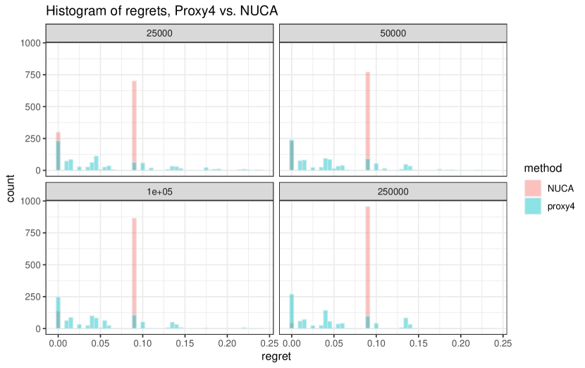
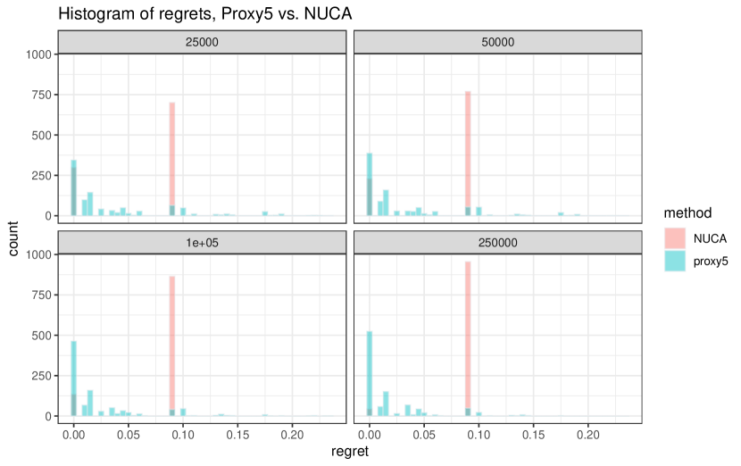
Figure 4: Regret comparisons between the NUCA estimator and the proxy estimators fit with different orders of interactions. From clockwise, 4,5, 7, and 8.

E.4 Exact details about the data-generating mechanism

We explicitly describe how the data were generated. In the following tables, for each of the 11 variables, we report the probability (up to 5 decimals) that the variable takes value 1 conditional on the value of their “parents” in Figure 1.

$U_{0}$	prob
1	0.61022

Table 2: Probability for $U_{0}$

$Y_{0}$	$U_{0}$	prob
1	0	0.52336
1	1	0.89644

Table 3: Probabilities for $Y_{0}\mid U_{0}$

$Z_{1}$	$U_{0}$	$Y_{0}$	prob
1	0	0	0.31885
1	1	0	0.08911
1	0	1	0.48126
1	1	1	0.66501

Table 4: Probabilities for $Z_{1}\mid U_{0},Y_{0}$

$A_{1}$	$Z_{1}$	$U_{0}$	$Y_{0}$	prob
1	0	0	0	0.54260
1	1	0	0	0.51091
1	0	1	0	0.45540
1	1	1	0	0.90720
1	0	0	1	0.65610
1	1	0	1	0.61606
1	0	1	1	0.47284
1	1	1	1	0.08915

Table 5: Probabilities for $A_{1}\mid Z_{1},U_{0},Y_{0}$

$W_{1}$	$U_{0}$	$Y_{0}$	prob
1	0	0	0.57083
1	1	0	0.77526
1	0	1	0.36461
1	1	1	0.87968

Table 6: Probabilities for $W_{1}\mid U_{0},Y_{0}$

$U_{1}$	$A_{1}$	$U_{0}$	$Y_{0}$	prob
1	0	0	0	0.87127
1	1	0	0	0.12769
1	0	1	0	0.39382
1	1	1	0	0.13824
1	0	0	1	0.89969
1	1	0	1	0.91185
1	0	1	1	0.44446
1	1	1	1	0.47431

Table 7: Probabilities for $U_{1}\mid A_{1},U_{0},Y_{0}$

$Y_{1}$	$A_{1}$	$W_{1}$	$U_{0}$	$Y_{0}$	prob
1	0	0	0	0	0.17216
1	1	0	0	0	0.40592
1	0	1	0	0	0.63933
1	1	1	0	0	0.08950
1	0	0	1	0	0.90824
1	1	0	1	0	0.27227
1	0	1	1	0	0.69990
1	1	1	1	0	0.79465
1	0	0	0	1	0.86302
1	1	0	0	1	0.08880
1	0	1	0	1	0.79623
1	1	1	0	1	0.83789
1	0	0	1	1	0.32020
1	1	0	1	1	0.17708
1	0	1	1	1	0.91378
1	1	1	1	1	0.12645

Table 8: Probabilities for $Y_{1}\mid A_{1},W_{1},U_{0},Y_{0}$

$Z_{2}$	$Y_{1}$	$U_{1}$	$A_{1}$	$Z_{1}$	$U_{0}$	$Y_{0}$	prob
1	0	0	0	0	0	0	0.10937
1	1	0	0	0	0	0	0.88783
1	0	1	0	0	0	0	0.83671
1	1	1	0	0	0	0	0.39415
1	0	0	1	0	0	0	0.41017
1	1	0	1	0	0	0	0.15292
1	0	1	1	0	0	0	0.15259
1	1	1	1	0	0	0	0.62252
1	0	0	0	1	0	0	0.10937
1	1	0	0	1	0	0	0.88783
1	0	1	0	1	0	0	0.83671
1	1	1	0	1	0	0	0.39415
1	0	0	1	1	0	0	0.41017
1	1	0	1	1	0	0	0.15292
1	0	1	1	1	0	0	0.15259
1	1	1	1	1	0	0	0.62252
1	0	0	0	0	1	0	0.10937
1	1	0	0	0	1	0	0.88783
1	0	1	0	0	1	0	0.83671
1	1	1	0	0	1	0	0.39415
1	0	0	1	0	1	0	0.41017
1	1	0	1	0	1	0	0.15292
1	0	1	1	0	1	0	0.15259
1	1	1	1	0	1	0	0.62252
1	0	0	0	1	1	0	0.10937
1	1	0	0	1	1	0	0.88783
1	0	1	0	1	1	0	0.83671
1	1	1	0	1	1	0	0.39415
1	0	0	1	1	1	0	0.41017
1	1	0	1	1	1	0	0.15292
1	0	1	1	1	1	0	0.15259
1	1	1	1	1	1	0	0.62252
1	0	0	0	0	0	1	0.10937
1	1	0	0	0	0	1	0.88783
1	0	1	0	0	0	1	0.83671
1	1	1	0	0	0	1	0.39415
1	0	0	1	0	0	1	0.41017
1	1	0	1	0	0	1	0.15292
1	0	1	1	0	0	1	0.15259
1	1	1	1	0	0	1	0.62252
1	0	0	0	1	0	1	0.10937
1	1	0	0	1	0	1	0.88783
1	0	1	0	1	0	1	0.83671
1	1	1	0	1	0	1	0.39415
1	0	0	1	1	0	1	0.41017
1	1	0	1	1	0	1	0.15292
1	0	1	1	1	0	1	0.15259
1	1	1	1	1	0	1	0.62252
1	0	0	0	0	1	1	0.10937
1	1	0	0	0	1	1	0.88783
1	0	1	0	0	1	1	0.83671
1	1	1	0	0	1	1	0.39415
1	0	0	1	0	1	1	0.41017
1	1	0	1	0	1	1	0.15292
1	0	1	1	0	1	1	0.15259
1	1	1	1	0	1	1	0.62252
1	0	0	0	1	1	1	0.10937
1	1	0	0	1	1	1	0.88783
1	0	1	0	1	1	1	0.83671
1	1	1	0	1	1	1	0.39415
1	0	0	1	1	1	1	0.41017
1	1	0	1	1	1	1	0.15292
1	0	1	1	1	1	1	0.15259
1	1	1	1	1	1	1	0.62252

Table 9: Probabilities for $Z_{2}\mid Y_{1},U_{1},A_{1},Z_{1},U_{0},Y_{0}$

$A_{2}$	$Y_{1}$	$U_{1}$	$Z_{2}$	$A_{1}$	$Z_{1}$	$U_{0}$	$Y_{0}$	prob
1	0	0	0	0	0	0	0	0.78844
1	1	0	0	0	0	0	0	0.60115
1	0	1	0	0	0	0	0	0.08881
1	1	1	0	0	0	0	0	0.63576
1	0	0	1	0	0	0	0	0.85524
1	1	0	1	0	0	0	0	0.73526
1	0	1	1	0	0	0	0	0.09268
1	1	1	1	0	0	0	0	0.58536
1	0	0	0	1	0	0	0	0.49993
1	1	0	0	1	0	0	0	0.08874
1	0	1	0	1	0	0	0	0.90496
1	1	1	0	1	0	0	0	0.86962
1	0	0	1	1	0	0	0	0.91073
1	1	0	1	1	0	0	0	0.67629
1	0	1	1	1	0	0	0	0.37260
1	1	1	1	1	0	0	0	0.75385
1	0	0	0	0	1	0	0	0.66399
1	1	0	0	0	1	0	0	0.57538
1	0	1	0	0	1	0	0	0.90122
1	1	1	0	0	1	0	0	0.88859
1	0	0	1	0	1	0	0	0.90308
1	1	0	1	0	1	0	0	0.63660
1	0	1	1	0	1	0	0	0.89924
1	1	1	1	0	1	0	0	0.19656
1	0	0	0	1	1	0	0	0.08668
1	1	0	0	1	1	0	0	0.08903
1	0	1	0	1	1	0	0	0.32200
1	1	1	0	1	1	0	0	0.75079
1	0	0	1	1	1	0	0	0.40711
1	1	0	1	1	1	0	0	0.77500
1	0	1	1	1	1	0	0	0.08985
1	1	1	1	1	1	0	0	0.09233
1	0	0	0	0	0	1	0	0.22040
1	1	0	0	0	0	1	0	0.09998
1	0	1	0	0	0	1	0	0.76019
1	1	1	0	0	0	1	0	0.57212
1	0	0	1	0	0	1	0	0.79266
1	1	0	1	0	0	1	0	0.40393
1	0	1	1	0	0	1	0	0.40811
1	1	1	1	0	0	1	0	0.74520
1	0	0	0	1	0	1	0	0.42596
1	1	0	0	1	0	1	0	0.55895
1	0	1	0	1	0	1	0	0.85419
1	1	1	0	1	0	1	0	0.39810
1	0	0	1	1	0	1	0	0.41922
1	1	0	1	1	0	1	0	0.30981
1	0	1	1	1	0	1	0	0.47941
1	1	1	1	1	0	1	0	0.08919
1	0	0	0	0	1	1	0	0.34564
1	1	0	0	0	1	1	0	0.23967
1	0	1	0	0	1	1	0	0.83892
1	1	1	0	0	1	1	0	0.51803
1	0	0	1	0	1	1	0	0.72522
1	1	0	1	0	1	1	0	0.26203
1	0	1	1	0	1	1	0	0.58195
1	1	1	1	0	1	1	0	0.26636
1	0	0	0	1	1	1	0	0.55596
1	1	0	0	1	1	1	0	0.16445
1	0	1	0	1	1	1	0	0.18694
1	1	1	0	1	1	1	0	0.66467
1	0	0	1	1	1	1	0	0.26576
1	1	0	1	1	1	1	0	0.82847
1	0	1	1	1	1	1	0	0.47539
1	1	1	1	1	1	1	0	0.30195

Table 10: Probabilities for $A_{2}\mid Y_{1},U_{1},Z_{2},A_{1},Z_{1},U_{0},Y_{0}$, part 1

$A_{2}$	$Y_{1}$	$U_{1}$	$Z_{2}$	$A_{1}$	$Z_{1}$	$U_{0}$	$Y_{0}$	prob
1	0	0	0	0	0	0	1	0.68123
1	1	0	0	0	0	0	1	0.23966
1	0	1	0	0	0	0	1	0.67538
1	1	1	0	0	0	0	1	0.39953
1	0	0	1	0	0	0	1	0.86453
1	1	0	1	0	0	0	1	0.49816
1	0	1	1	0	0	0	1	0.56053
1	1	1	1	0	0	0	1	0.50820
1	0	0	0	1	0	0	1	0.78400
1	1	0	0	1	0	0	1	0.17413
1	0	1	0	1	0	0	1	0.38485
1	1	1	0	1	0	0	1	0.17792
1	0	0	1	1	0	0	1	0.15150
1	1	0	1	1	0	0	1	0.18026
1	0	1	1	1	0	0	1	0.15259
1	1	1	1	1	0	0	1	0.48665
1	0	0	0	0	1	0	1	0.43367
1	1	0	0	0	1	0	1	0.47962
1	0	1	0	0	1	0	1	0.65926
1	1	1	0	0	1	0	1	0.53693
1	0	0	1	0	1	0	1	0.43338
1	1	0	1	0	1	0	1	0.59161
1	0	1	1	0	1	0	1	0.19858
1	1	1	1	0	1	0	1	0.52214
1	0	0	0	1	1	0	1	0.09382
1	1	0	0	1	1	0	1	0.90123
1	0	1	0	1	1	0	1	0.53931
1	1	1	0	1	1	0	1	0.48958
1	0	0	1	1	1	0	1	0.85926
1	1	0	1	1	1	0	1	0.16868
1	0	1	1	1	1	0	1	0.10570
1	1	1	1	1	1	0	1	0.09081
1	0	0	0	0	0	1	1	0.13595
1	1	0	0	0	0	1	1	0.14878
1	0	1	0	0	0	1	1	0.69362
1	1	1	0	0	0	1	1	0.43621
1	0	0	1	0	0	1	1	0.73305
1	1	0	1	0	0	1	1	0.85413
1	0	1	1	0	0	1	1	0.17952
1	1	1	1	0	0	1	1	0.14278
1	0	0	0	1	0	1	1	0.29845
1	1	0	0	1	0	1	1	0.18472
1	0	1	0	1	0	1	1	0.84328
1	1	1	0	1	0	1	1	0.91169
1	0	0	1	1	0	1	1	0.56811
1	1	0	1	1	0	1	1	0.28000
1	0	1	1	1	0	1	1	0.10286
1	1	1	1	1	0	1	1	0.78237
1	0	0	0	0	1	1	1	0.83464
1	1	0	0	0	1	1	1	0.90013
1	0	1	0	0	1	1	1	0.90646
1	1	1	0	0	1	1	1	0.25556
1	0	0	1	0	1	1	1	0.56302
1	1	0	1	0	1	1	1	0.45816
1	0	1	1	0	1	1	1	0.33779
1	1	1	1	0	1	1	1	0.36126
1	0	0	0	1	1	1	1	0.26726
1	1	0	0	1	1	1	1	0.48403
1	0	1	0	1	1	1	1	0.88958
1	1	1	0	1	1	1	1	0.09453
1	0	0	1	1	1	1	1	0.16005
1	1	0	1	1	1	1	1	0.12803
1	0	1	1	1	1	1	1	0.09346
1	1	1	1	1	1	1	1	0.64677

Table 11: Probabilities for $A_{2}\mid Y_{1},U_{1},Z_{2},A_{1},Z_{1},U_{0},Y_{0}$, part 2

$W_{2}$	$Y_{1}$	$U_{1}$	$W_{1}$	$U_{0}$	$Y_{0}$	prob
1	0	0	0	0	0	0.57628
1	1	0	0	0	0	0.08505
1	0	1	0	0	0	0.66033
1	1	1	0	0	0	0.40567
1	0	0	1	0	0	0.57628
1	1	0	1	0	0	0.08505
1	0	1	1	0	0	0.66033
1	1	1	1	0	0	0.40567
1	0	0	0	1	0	0.57628
1	1	0	0	1	0	0.08505
1	0	1	0	1	0	0.66033
1	1	1	0	1	0	0.40567
1	0	0	1	1	0	0.57628
1	1	0	1	1	0	0.08505
1	0	1	1	1	0	0.66033
1	1	1	1	1	0	0.40567
1	0	0	0	0	1	0.57628
1	1	0	0	0	1	0.08505
1	0	1	0	0	1	0.66033
1	1	1	0	0	1	0.40567
1	0	0	1	0	1	0.57628
1	1	0	1	0	1	0.08505
1	0	1	1	0	1	0.66033
1	1	1	1	0	1	0.40567
1	0	0	0	1	1	0.57628
1	1	0	0	1	1	0.08505
1	0	1	0	1	1	0.66033
1	1	1	0	1	1	0.40567
1	0	0	1	1	1	0.57628
1	1	0	1	1	1	0.08505
1	0	1	1	1	1	0.66033
1	1	1	1	1	1	0.40567

Table 12: Probabilities for $W_{2}\mid Y_{1},U_{1},W_{1},U_{0},Y_{0}$

$Y_{2}$	$Y_{1}$	$A_{2}$	$U_{1}$	$W_{2}$	$A_{1}$	$W_{1}$	$U_{0}$	$Y_{0}$	prob
1	0	0	0	0	0	0	0	0	0.12652
1	1	0	0	0	0	0	0	0	0.41111
1	0	1	0	0	0	0	0	0	0.17325
1	1	1	0	0	0	0	0	0	0.25998
1	0	0	1	0	0	0	0	0	0.66491
1	1	0	1	0	0	0	0	0	0.11604
1	0	1	1	0	0	0	0	0	0.50372
1	1	1	1	0	0	0	0	0	0.30775
1	0	0	0	1	0	0	0	0	0.18514
1	1	0	0	1	0	0	0	0	0.90741
1	0	1	0	1	0	0	0	0	0.62827
1	1	1	0	1	0	0	0	0	0.20048
1	0	0	1	1	0	0	0	0	0.24835
1	1	0	1	1	0	0	0	0	0.69348
1	0	1	1	1	0	0	0	0	0.83572
1	1	1	1	1	0	0	0	0	0.21449
1	0	0	0	0	1	0	0	0	0.59396
1	1	0	0	0	1	0	0	0	0.22567
1	0	1	0	0	1	0	0	0	0.34817
1	1	1	0	0	1	0	0	0	0.25434
1	0	0	1	0	1	0	0	0	0.50533
1	1	0	1	0	1	0	0	0	0.62788
1	0	1	1	0	1	0	0	0	0.50256
1	1	1	1	0	1	0	0	0	0.09160
1	0	0	0	1	1	0	0	0	0.08856
1	1	0	0	1	1	0	0	0	0.47210
1	0	1	0	1	1	0	0	0	0.18709
1	1	1	0	1	1	0	0	0	0.91046
1	0	0	1	1	1	0	0	0	0.09462
1	1	0	1	1	1	0	0	0	0.34301
1	0	1	1	1	1	0	0	0	0.28264
1	1	1	1	1	1	0	0	0	0.18453
1	0	0	0	0	0	1	0	0	0.12652
1	1	0	0	0	0	1	0	0	0.41111
1	0	1	0	0	0	1	0	0	0.17325
1	1	1	0	0	0	1	0	0	0.25998
1	0	0	1	0	0	1	0	0	0.66491
1	1	0	1	0	0	1	0	0	0.11604
1	0	1	1	0	0	1	0	0	0.50372
1	1	1	1	0	0	1	0	0	0.30775
1	0	0	0	1	0	1	0	0	0.18514
1	1	0	0	1	0	1	0	0	0.90741
1	0	1	0	1	0	1	0	0	0.62827
1	1	1	0	1	0	1	0	0	0.20048
1	0	0	1	1	0	1	0	0	0.24835
1	1	0	1	1	0	1	0	0	0.69348
1	0	1	1	1	0	1	0	0	0.83572
1	1	1	1	1	0	1	0	0	0.21449
1	0	0	0	0	1	1	0	0	0.59396
1	1	0	0	0	1	1	0	0	0.22567
1	0	1	0	0	1	1	0	0	0.34817
1	1	1	0	0	1	1	0	0	0.25434
1	0	0	1	0	1	1	0	0	0.50533
1	1	0	1	0	1	1	0	0	0.62788
1	0	1	1	0	1	1	0	0	0.50256
1	1	1	1	0	1	1	0	0	0.09160
1	0	0	0	1	1	1	0	0	0.08856
1	1	0	0	1	1	1	0	0	0.47210
1	0	1	0	1	1	1	0	0	0.18709
1	1	1	0	1	1	1	0	0	0.91046
1	0	0	1	1	1	1	0	0	0.09462
1	1	0	1	1	1	1	0	0	0.34301
1	0	1	1	1	1	1	0	0	0.28264
1	1	1	1	1	1	1	0	0	0.18453

Table 13: Probabilities for $Y_{2}\mid Y_{1},A_{2},U_{1},W_{2},A_{1},W_{1},U_{0},Y_{0}$, part 1

$Y_{2}$	$Y_{1}$	$A_{2}$	$U_{1}$	$W_{2}$	$A_{1}$	$W_{1}$	$U_{0}$	$Y_{0}$	prob
1	0	0	0	0	0	0	1	0	0.66090
1	1	0	0	0	0	0	1	0	0.65430
1	0	1	0	0	0	0	1	0	0.70659
1	1	1	0	0	0	0	1	0	0.44891
1	0	0	1	0	0	0	1	0	0.58325
1	1	0	1	0	0	0	1	0	0.32500
1	0	1	1	0	0	0	1	0	0.20901
1	1	1	1	0	0	0	1	0	0.09676
1	0	0	0	1	0	0	1	0	0.48315
1	1	0	0	1	0	0	1	0	0.40259
1	0	1	0	1	0	0	1	0	0.81642
1	1	1	0	1	0	0	1	0	0.68273
1	0	0	1	1	0	0	1	0	0.37558
1	1	0	1	1	0	0	1	0	0.09888
1	0	1	1	1	0	0	1	0	0.83432
1	1	1	1	1	0	0	1	0	0.85309
1	0	0	0	0	1	0	1	0	0.63615
1	1	0	0	0	1	0	1	0	0.71703
1	0	1	0	0	1	0	1	0	0.91469
1	1	1	0	0	1	0	1	0	0.60636
1	0	0	1	0	1	0	1	0	0.17402
1	1	0	1	0	1	0	1	0	0.86691
1	0	1	1	0	1	0	1	0	0.91106
1	1	1	1	0	1	0	1	0	0.78781
1	0	0	0	1	1	0	1	0	0.09119
1	1	0	0	1	1	0	1	0	0.89678
1	0	1	0	1	1	0	1	0	0.25728
1	1	1	0	1	1	0	1	0	0.88819
1	0	0	1	1	1	0	1	0	0.61229
1	1	0	1	1	1	0	1	0	0.16243
1	0	1	1	1	1	0	1	0	0.90677
1	1	1	1	1	1	0	1	0	0.08906
1	0	0	0	0	0	1	1	0	0.66090
1	1	0	0	0	0	1	1	0	0.65430
1	0	1	0	0	0	1	1	0	0.70659
1	1	1	0	0	0	1	1	0	0.44891
1	0	0	1	0	0	1	1	0	0.58325
1	1	0	1	0	0	1	1	0	0.32500
1	0	1	1	0	0	1	1	0	0.20901
1	1	1	1	0	0	1	1	0	0.09676
1	0	0	0	1	0	1	1	0	0.48315
1	1	0	0	1	0	1	1	0	0.40259
1	0	1	0	1	0	1	1	0	0.81642
1	1	1	0	1	0	1	1	0	0.68273
1	0	0	1	1	0	1	1	0	0.37558
1	1	0	1	1	0	1	1	0	0.09888
1	0	1	1	1	0	1	1	0	0.83432
1	1	1	1	1	0	1	1	0	0.85309
1	0	0	0	0	1	1	1	0	0.63615
1	1	0	0	0	1	1	1	0	0.71703
1	0	1	0	0	1	1	1	0	0.91469
1	1	1	0	0	1	1	1	0	0.60636
1	0	0	1	0	1	1	1	0	0.17402
1	1	0	1	0	1	1	1	0	0.86691
1	0	1	1	0	1	1	1	0	0.91106
1	1	1	1	0	1	1	1	0	0.78781
1	0	0	0	1	1	1	1	0	0.09119
1	1	0	0	1	1	1	1	0	0.89678
1	0	1	0	1	1	1	1	0	0.25728
1	1	1	0	1	1	1	1	0	0.88819
1	0	0	1	1	1	1	1	0	0.61229
1	1	0	1	1	1	1	1	0	0.16243
1	0	1	1	1	1	1	1	0	0.90677
1	1	1	1	1	1	1	1	0	0.08906

Table 14: Probabilities for $Y_{2}\mid Y_{1},A_{2},U_{1},W_{2},A_{1},W_{1},U_{0},Y_{0}$, part 2

$Y_{2}$	$Y_{1}$	$A_{2}$	$U_{1}$	$W_{2}$	$A_{1}$	$W_{1}$	$U_{0}$	$Y_{0}$	prob
1	0	0	0	0	0	0	0	1	0.15589
1	1	0	0	0	0	0	0	1	0.46859
1	0	1	0	0	0	0	0	1	0.84267
1	1	1	0	0	0	0	0	1	0.43580
1	0	0	1	0	0	0	0	1	0.65379
1	1	0	1	0	0	0	0	1	0.91450
1	0	1	1	0	0	0	0	1	0.87363
1	1	1	1	0	0	0	0	1	0.37705
1	0	0	0	1	0	0	0	1	0.12005
1	1	0	0	1	0	0	0	1	0.12517
1	0	1	0	1	0	0	0	1	0.09279
1	1	1	0	1	0	0	0	1	0.47729
1	0	0	1	1	0	0	0	1	0.63574
1	1	0	1	1	0	0	0	1	0.28424
1	0	1	1	1	0	0	0	1	0.34422
1	1	1	1	1	0	0	0	1	0.23074
1	0	0	0	0	1	0	0	1	0.39316
1	1	0	0	0	1	0	0	1	0.72255
1	0	1	0	0	1	0	0	1	0.24771
1	1	1	0	0	1	0	0	1	0.14739
1	0	0	1	0	1	0	0	1	0.35182
1	1	0	1	0	1	0	0	1	0.65767
1	0	1	1	0	1	0	0	1	0.13766
1	1	1	1	0	1	0	0	1	0.75026
1	0	0	0	1	1	0	0	1	0.09609
1	1	0	0	1	1	0	0	1	0.74559
1	0	1	0	1	1	0	0	1	0.46586
1	1	1	0	1	1	0	0	1	0.91125
1	0	0	1	1	1	0	0	1	0.63671
1	1	0	1	1	1	0	0	1	0.45222
1	0	1	1	1	1	0	0	1	0.71285
1	1	1	1	1	1	0	0	1	0.89711
1	0	0	0	0	0	1	0	1	0.15589
1	1	0	0	0	0	1	0	1	0.46859
1	0	1	0	0	0	1	0	1	0.84267
1	1	1	0	0	0	1	0	1	0.43580
1	0	0	1	0	0	1	0	1	0.65379
1	1	0	1	0	0	1	0	1	0.91450
1	0	1	1	0	0	1	0	1	0.87363
1	1	1	1	0	0	1	0	1	0.37705
1	0	0	0	1	0	1	0	1	0.12005
1	1	0	0	1	0	1	0	1	0.12517
1	0	1	0	1	0	1	0	1	0.09279
1	1	1	0	1	0	1	0	1	0.47729
1	0	0	1	1	0	1	0	1	0.63574
1	1	0	1	1	0	1	0	1	0.28424
1	0	1	1	1	0	1	0	1	0.34422
1	1	1	1	1	0	1	0	1	0.23074
1	0	0	0	0	1	1	0	1	0.39316
1	1	0	0	0	1	1	0	1	0.72255
1	0	1	0	0	1	1	0	1	0.24771
1	1	1	0	0	1	1	0	1	0.14739
1	0	0	1	0	1	1	0	1	0.35182
1	1	0	1	0	1	1	0	1	0.65767
1	0	1	1	0	1	1	0	1	0.13766
1	1	1	1	0	1	1	0	1	0.75026
1	0	0	0	1	1	1	0	1	0.09609
1	1	0	0	1	1	1	0	1	0.74559
1	0	1	0	1	1	1	0	1	0.46586
1	1	1	0	1	1	1	0	1	0.91125
1	0	0	1	1	1	1	0	1	0.63671
1	1	0	1	1	1	1	0	1	0.45222
1	0	1	1	1	1	1	0	1	0.71285
1	1	1	1	1	1	1	0	1	0.89711

Table 15: Probabilities for $Y_{2}\mid Y_{1},A_{2},U_{1},W_{2},A_{1},W_{1},U_{0},Y_{0}$, part 3

$Y_{2}$	$Y_{1}$	$A_{2}$	$U_{1}$	$W_{2}$	$A_{1}$	$W_{1}$	$U_{0}$	$Y_{0}$	prob
1	0	0	0	0	0	0	1	1	0.40100
1	1	0	0	0	0	0	1	1	0.17102
1	0	1	0	0	0	0	1	1	0.84896
1	1	1	0	0	0	0	1	1	0.90283
1	0	0	1	0	0	0	1	1	0.63803
1	1	0	1	0	0	0	1	1	0.43280
1	0	1	1	0	0	0	1	1	0.55443
1	1	1	1	0	0	0	1	1	0.53318
1	0	0	0	1	0	0	1	1	0.09312
1	1	0	0	1	0	0	1	1	0.47655
1	0	1	0	1	0	0	1	1	0.63378
1	1	1	0	1	0	0	1	1	0.09191
1	0	0	1	1	0	0	1	1	0.64215
1	1	0	1	1	0	0	1	1	0.58728
1	0	1	1	1	0	0	1	1	0.10078
1	1	1	1	1	0	0	1	1	0.09889
1	0	0	0	0	1	0	1	1	0.38510
1	1	0	0	0	1	0	1	1	0.41662
1	0	1	0	0	1	0	1	1	0.38945
1	1	1	0	0	1	0	1	1	0.47669
1	0	0	1	0	1	0	1	1	0.57501
1	1	0	1	0	1	0	1	1	0.91348
1	0	1	1	0	1	0	1	1	0.34647
1	1	1	1	0	1	0	1	1	0.90096
1	0	0	0	1	1	0	1	1	0.75558
1	1	0	0	1	1	0	1	1	0.17970
1	0	1	0	1	1	0	1	1	0.14273
1	1	1	0	1	1	0	1	1	0.35391
1	0	0	1	1	1	0	1	1	0.90934
1	1	0	1	1	1	0	1	1	0.62472
1	0	1	1	1	1	0	1	1	0.43601
1	1	1	1	1	1	0	1	1	0.63247
1	0	0	0	0	0	1	1	1	0.40100
1	1	0	0	0	0	1	1	1	0.17102
1	0	1	0	0	0	1	1	1	0.84896
1	1	1	0	0	0	1	1	1	0.90283
1	0	0	1	0	0	1	1	1	0.63803
1	1	0	1	0	0	1	1	1	0.43280
1	0	1	1	0	0	1	1	1	0.55443
1	1	1	1	0	0	1	1	1	0.53318
1	0	0	0	1	0	1	1	1	0.09312
1	1	0	0	1	0	1	1	1	0.47655
1	0	1	0	1	0	1	1	1	0.63378
1	1	1	0	1	0	1	1	1	0.09191
1	0	0	1	1	0	1	1	1	0.64215
1	1	0	1	1	0	1	1	1	0.58728
1	0	1	1	1	0	1	1	1	0.10078
1	1	1	1	1	0	1	1	1	0.09889
1	0	0	0	0	1	1	1	1	0.38510
1	1	0	0	0	1	1	1	1	0.41662
1	0	1	0	0	1	1	1	1	0.38945
1	1	1	0	0	1	1	1	1	0.47669
1	0	0	1	0	1	1	1	1	0.57501
1	1	0	1	0	1	1	1	1	0.91348
1	0	1	1	0	1	1	1	1	0.34647
1	1	1	1	0	1	1	1	1	0.90096
1	0	0	0	1	1	1	1	1	0.75558
1	1	0	0	1	1	1	1	1	0.17970
1	0	1	0	1	1	1	1	1	0.14273
1	1	1	0	1	1	1	1	1	0.35391
1	0	0	1	1	1	1	1	1	0.90934
1	1	0	1	1	1	1	1	1	0.62472
1	0	1	1	1	1	1	1	1	0.43601
1	1	1	1	1	1	1	1	1	0.63247

Table 16: Probabilities for $Y_{2}\mid Y_{1},A_{2},U_{1},W_{2},A_{1},W_{1},U_{0},Y_{0}$, part 4

References

- Bennett and Kallus [2021] A. Bennett and N. Kallus. Proximal Reinforcement Learning: Efficient Off-Policy Evaluation in Partially Observed Markov Decision Processes. arXiv, 10 2021. URL http://arxiv.org/abs/2110.15332.
- Bennett et al. [2023] A. Bennett, N. Kallus, X. Mao, W. Newey, V. Syrgkanis, and M. Uehara. Minimax Instrumental Variable Regression and L2 Convergence Guarantees without Identification or Closedness. Proceedings of Thirty Sixth Conference on Learning Theory, PMLR, 195:2291–2318, 2023. ISSN 26403498.
- Bruns-Smith and Zhou [2023] D. Bruns-Smith and A. Zhou. Robust Fitted-Q-Evaluation and Iteration under Sequentially Exogenous Unobserved Confounders. arXiv, 2 2023. URL http://arxiv.org/abs/2302.00662.
- Carrasco et al. [2007] M. Carrasco, J.-P. Florens, and E. Renault. Chapter 77 Linear Inverse Problems in Structural Econometrics Estimation Based on Spectral Decomposition and Regularization. pages 5633–5751. 2007. doi: 10.1016/S1573-4412(07)06077-1. URL https://linkinghub.elsevier.com/retrieve/pii/S1573441207060771.
- Chen and Zhang [2023] S. Chen and B. Zhang. Estimating and improving dynamic treatment regimes with a time-varying instrumental variable. Journal of the Royal Statistical Society. Series B: Statistical Methodology, 85(2):427–453, 4 2023. ISSN 14679868. doi: 10.1093/jrsssb/qkad011.
- Dukes et al. [2023] O. Dukes, I. Shpitser, and E. J. Tchetgen Tchetgen. Proximal mediation analysis. Biometrika, 110(4):973–987, 11 2023. ISSN 0006-3444. doi: 10.1093/biomet/asad015.
- Han [2021] S. Han. Identification in nonparametric models for dynamic treatment effects. Journal of Econometrics, 225(2):132–147, 12 2021. ISSN 18726895. doi: 10.1016/j.jeconom.2019.08.014.
- Han [2023] S. Han. Optimal Dynamic Treatment Regimes and Partial Welfare Ordering. Journal of the American Statistical Association, 2023. ISSN 1537274X. doi: 10.1080/01621459.2023.2238941.
- Kress [1999] R. Kress. Linear Integral Equations, volume 82 of Applied Mathematical Sciences. Springer New York, New York, NY, 1999. ISBN 978-1-4612-6817-8. doi: 10.1007/978-1-4612-0559-3. URL http://link.springer.com/10.1007/978-1-4612-0559-3.
- Miao et al. [2022] R. Miao, Z. Qi, and X. Zhang. Off-Policy Evaluation for Episodic Partially Observable Markov Decision Processes under Non-Parametric Models. In NeurIPS, 2022.
- Miao et al. [2018] W. Miao, Z. Geng, and E. J. Tchetgen Tchetgen. Identifying causal effects with proxy variables of an unmeasured confounder. Biometrika, 105(4):987–993, 12 2018. ISSN 14643510. doi: 10.1093/biomet/asy038.
- Michael et al. [2023] H. Michael, Y. Cui, S. A. Lorch, and E. J. Tchetgen Tchetgen. Instrumental Variable Estimation of Marginal Structural Mean Models for Time-Varying Treatment. Journal of the American Statistical Association, pages 1–12, 4 2023. ISSN 0162-1459. doi: 10.1080/01621459.2023.2183131.
- Murphy [2003] S. A. Murphy. Optimal Dynamic Treatment Regimes. Journal of the Royal Statistical Society. Series B (Statistical Methodology), 65(2):331–366, 2003. URL https://www.jstor.org/stable/3647509?seq=1&cid=pdf-.
- Qi et al. [2023] Z. Qi, R. Miao, and X. Zhang. Proximal Learning for Individualized Treatment Regimes Under Unmeasured Confounding. Journal of the American Statistical Association, 2023. ISSN 1537274X. doi: 10.1080/01621459.2022.2147841.
- Robins [1986] J. Robins. A NEW APPROACH TO CAUSAL INFERENCE IN MORTALITY STUDIES WITH A SUSTAINED EXPOSURE PERIOD-APPLICATION TO CONTROL OF THE HEALTHY WORKER SURVIVOR EFFECT. Mathematical Modeling, 7:1393–1512, 1986.
- Shen and Cui [2022] T. Shen and Y. Cui. Optimal Treatment Regimes for Proximal Causal Learning. arXiv, 12 2022. URL http://arxiv.org/abs/2212.09494.
- Shi et al. [2020a] X. Shi, W. Miao, J. C. Nelson, and E. J. Tchetgen Tchetgen. Multiply Robust Causal Inference with Double-Negative Control Adjustment for Categorical Unmeasured Confounding. Journal of the Royal Statistical Society Series B: Statistical Methodology, 82(2):521–540, 4 2020a. ISSN 1369-7412. doi: 10.1111/rssb.12361.
- Shi et al. [2020b] X. Shi, W. Miao, and E. T. Tchetgen. A Selective Review of Negative Control Methods in Epidemiology. Current Epidemiology Reports, 7(4):190–202, 12 2020b. ISSN 2196-2995. doi: 10.1007/s40471-020-00243-4. URL https://link.springer.com/10.1007/s40471-020-00243-4.
- Singh [2021] R. Singh. A Finite Sample Theorem for Longitudinal Causal Inference with Machine Learning: Long Term, Dynamic, and Mediated Effects. arXiv, 12 2021. URL http://arxiv.org/abs/2112.14249.
- Tan [2006] Z. Tan. A distributional approach for causal inference using propensity scores. Journal of the American Statistical Association, 101(476):1619–1637, 12 2006. ISSN 01621459. doi: 10.1198/016214506000000023.
- Tchetgen Tchetgen et al. [2024] E. Tchetgen Tchetgen, A. Ying, Y. Cui, X. Shi, and W. Miao. An Introduction to Proximal Causal Inference. Statistical Science, 2024.
- Tsiatis et al. [2019] A. A. Tsiatis, M. Davidian, S. T. Holloway, and E. B. Laber. Dynamic Treatment Regimes. Chapman and Hall/CRC, Boca Raton : Chapman and Hall/CRC, 2020. — Series: Chapman & Hall/CRC monographs on statistics and applied probability, 12 2019. ISBN 9780429192692. doi: 10.1201/9780429192692.
- Ying et al. [2023] A. Ying, W. Miao, X. Shi, and E. J. Tchetgen Tchetgen. Proximal Causal Inference for Complex Longitudinal Studies. Journal of the Royal Statistical Society Series B: Statistical Methodology, 85(3):684–704, 12 2023. ISSN 14643510. doi: 10.1093/biomet/asy038.
- Zhang et al. [2023] J. Zhang, W. Li, W. Miao, and E. Tchetgen Tchetgen. Proximal causal inference without uniqueness assumptions. Statistics & Probability Letters, 198:109836, 7 2023. ISSN 01677152. doi: 10.1016/j.spl.2023.109836. URL https://linkinghub.elsevier.com/retrieve/pii/S0167715223000603.