Energy-efficiency Limits on Training AI Systems using Learning-in-Memory

Abstract

Learning-in-memory (LIM) is a recently proposed paradigm to overcome fundamental memory bottlenecks in training machine learning systems. While compute-in-memory (CIM) approaches can address the so-called memory-wall (i.e. energy dissipated due to repeated memory read access) they are agnostic to the energy dissipated due to repeated memory writes at the precision required for training (the update-wall), and they don’t account for the energy dissipated when transferring information between short-term and long-term memories (the consolidation-wall). The LIM paradigm proposes that these bottlenecks, too, can be overcome if the energy barrier of physical memories is adaptively modulated such that the dynamics of memory updates and consolidation match the Lyapunov dynamics of gradient-descent training of an AI model. In this paper, we derive new theoretical lower bounds on energy dissipation when training AI systems using different LIM approaches. The analysis presented here is model-agnostic and highlights the trade-off between energy efficiency and the speed of training. The resulting non-equilibrium energy-efficiency bounds have a similar flavor as that of Landauer’s energy-dissipation bounds. We also extend these limits by taking into account the number of floating-point operations (FLOPs) used for training, the size of the AI model, and the precision of the training parameters. Our projections suggest that the energy-dissipation lower-bound to train a brain scale AI system (comprising of $10^{15}$ parameters) using LIM is $10^{8}\sim 10^{9}$ Joules, which is on the same magnitude the Landauer’s adiabatic lower-bound and $6$ to $7$ orders of magnitude lower than the projections obtained using state-of-the-art AI accelerator hardware lower-bounds.

Keywords AI  $\cdot$ Training  $\cdot$ Energy-efficiency  $\cdot$ Landauer’s limit  $\cdot$ Learning-in-memory

1 Introduction

In recent years, the increasing success of artificial intelligence (AI) systems has been marked by rapid growth in the size and complexity of the underlying mathematical models[1]. This trend has not only been driven by the availability of large data sets used for training, but also by advances in hardware accelerators that can train these complex AI models within realistic time, energy, and cost constraints. However, their progress has also highlighted significant challenges on the long road towards general AI or brain-scale AI systems [2, 3]. This is apparent in the trends shown in Figure 1, which relates the reported number of floating-point operations (FLOPS) required to train various AI systems of different sizes to the number of trainable parameters. For smaller-size models (number of parameters less than ${10}^{9}$), the number of training FLOPS is used to scale quadratically with the number of parameters. However, this cost has become prohibitive for large-scale AI models, so significant effort in recent years has been devoted to finding more efficient training methods. The scaling for these newer state-of-the-art large language models (LLMs), depicted in Figure 1, appears to be linear. But even this favorable trend becomes prohibitively costly when extrapolated to the number of FLOPS (around ${10}^{28}$) that would be required to train a brain-scale AI system comprising ${10}^{15}$ parameters, which roughly equals the number of synapses in a human brain [4, 5].

Figure 1: Trends showing the growth of computational and energy needs for training AI models [6], which has been used to predict the ${10}^{28}$ FLOPs and ${10}^{17}\text{\,}\mathrm{J}$ of energy that would be needed to train a brain-scale AI model.

To estimate the total energy required to train such a system, we can relate its energy consumption to the number of FLOPS performed during training, which appears to be a linear relationship, as depicted in Figure 1, where we have used reported energy dissipation metrics for several AI systems [7, 8, 9] for benchmarking. Extrapolating this FLOPs-to-energy relation to a brain-scale AI model, as shown in Figure 1(b), the energy dissipated to train the model can be estimated to be ${10}^{17}\text{\,}\mathrm{J}$ or equivalently $2.78\text{\times}{10}^{7}\text{\,}\mathrm{MW}\text{\,}\mathrm{h}$. For reference, this energy estimate equals the energy consumption of a typical U.S. household for 2,500,000 years [10, 3]. Such an unsustainable energy footprint for training AI systems in general, and in particular for deep-learning systems, has also been predicted in recent empirical reports and analyses [11]. Also, note that these energy dissipation estimates correspond to only a single round of training, whereas many commercial applications of large-scale AI models or their use in scientific discovery may require multiple rounds of training [12, 13, 14], further exacerbating the total energy footprint.

Similar to many other large computing tasks, the energy footprint for training AI systems arises primarily from memory bottlenecks [15, 16]. Unlike AI inference, AI training involves searching over a large set of parameters and hence requires repeated memorization, caching, and pruning. For a conventional Von-Neumann computer architecture, the compute and memory units are physically separated. Thus, frequent parameter updates across the physical memory hierarchy contribute to significant energy dissipation, which can be categorized into three performance walls [17]: the memory-wall, the update-wall, and the consolidation-wall, all of which are illustrated in Figure 2abc. The memory-wall [16] arises because of energy-dissipation due to the frequent data transfers between the computation and storage units across a memory bus (depicted in Figure 2a). In emerging AI hardware, the memory-wall is addressed by co-locating the memory and computation functional units [18, 19], in part motivated by neurobiology [20]. This compute-in-memory (CIM) paradigm has also been proposed for implementing ultra-energy-efficient neuromorphic systems [21] and analog classifiers [22] where physical synapses (memory) within the neurons (compute units) are embedded in a cross-bar architecture. While the CIM paradigm can significantly improve the energy efficiency for AI inference, unfortunately, the paradigm does not address the other two performance walls due to the energy dissipation caused by memory writes (the update-wall), nor due to data transfers across the memory hierarchy (the consolidation-wall). In fact, the reliance on non-volatile memory may exacerbate these problems. The update-wall arises because for most storage technology the energy dissipated during memory writes is significantly higher than the energy needed to read the contents of a memory [23]. This poses a particular challenge for the large number of memory writes and relatively high precision required for the parameter updates [24, 25] during AI training. The consolidation-wall arises due to the limited capacity of physical memory that can be integrated with or in proximity to the compute units [26, 27]. As a result, only some of the parameters of large AI models can be stored or cached locally, whereas the majority has to be moved and consolidated off-chip. Repeated access to this off-chip memory and the consolidation overhead in maintaining a working set of active parameters [28] across different levels of memory cache hierarchy present a significant source of energy-dissipation during AI training.

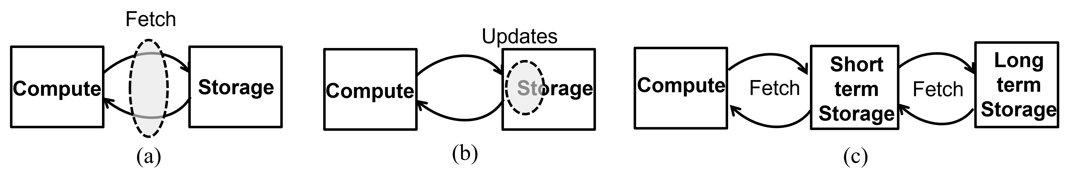
Figure 2: Performance walls that determine energy-efficiency of AI training (a) Memory-wall which arises due to frequent memory access by remote compute units; (b) Update-wall which arises due to high energy cost of memory writes at a required precision; (c) Consolidation-wall which arises due to limited memory capacity and hence repeated data transfers across different memory hierarchy (short-term and long-term storage).

Analogous to the CIM paradigm, can neurobiology also provide similar cues on how to address the update- and consolidation-walls? At a fundamental level the precision of biological synapses as storage elements is severely limited [29]. Despite this, some computations observed in neurobiology are surprisingly precise [30], which has been attributed to a combination of massive parallelism, redundancy, and stochastic encoding principles [31, 32]. In this framework, intrinsic randomness and thermal fluctuations in the synaptic devices not only aid in achieving higher precision during learning but also improve the energy efficiency through noise-exploitation [33]. Note that this paradigm of thermodynamics-driven (or Brownian) computing is not unique to biological synapses but has also been observed in other biological processes like DNA hybridization [34], and hence could be a key to address the update-wall. Furthermore, there is growing evidence that biological synapses are inherently complex high-dimensional dynamical systems themselves [35, 36] as opposed to the simple, static storage units that are typically assumed in neural networks. This neuromorphic viewpoint is supported by experimental evidence of metaplasticity observed in biological synapses [37, 38], where the synaptic plasticity (e.g. the ‘ease’ of updates) has been observed to vary depending on age and in a task-specific manner. Metaplasticity also plays a key role in neurobiological memory consolidation[39, 40], where short-term information stored in ‘volatile’, easy-to-update memory in the hippocampus is subsequently consolidated into long-term memory in the neocortex. Even though both of these spatially separated memory systems are characterized by short-term and long-term storage dynamics (similar to synthetic memory systems), they are tightly coupled to each other through distributed compute units (neurons).

Can the update- and consolidation-walls be addressed by locally adjusting the parameters of a physical memory? Recent work has demonstrated silicon-based metaplastic synapses that can not only be used to improve training energy-efficiency [41] but to achieve higher pattern storage capacity through memory consolidation [42]. The key premise is that if the physics of the memory elements can be exploited for parameter updates, computing, and memory consolidation, then the energy dissipated during training could be significantly reduced. At the physical level, the memory elements used in most AI hardware (for e.g. static random access memory or SRAM), are static in nature, i.e. discrete memory states $(..,W_{n-1},W_{n},..)$ over time $n$ are separated from each other by some static energy barrier $E^{0}$, as shown in Figure 3a. This energy barrier is generally chosen to be large enough to prevent memory leakage due to thermal fluctuations, especially during inference, when the memory needs to be non-volatile. When transitioning from state $W_{n-1}\rightarrow W_{n}$, the energy is irrevocably lost as shown in Figure 3b-c. Therefore, a learning/training algorithm that minimizes a loss-function $L(W)$ (as shown in Figure 3d) by adapting the weights in quantized steps (shown in Figure 3e) has to dissipate the energy $E^{0}$ for every update - irrespective of the dynamics of the optimization problem. From a thermodynamic point of view, one can view this energy cost arising from the need to keep the entropy of the learning trajectories in hardware close to zero. This is illustrated in Figure 3d using a single trajectory (denoted by red curve) from the initial state ${W}_{0}$ to the final state ${W}_{N}$.

However, if the energy barrier were modulated with dynamics that are coupled to the dynamics of the learning process, i.e. where the energy gradient $\Delta E$ changes with the algorithmic gradient $\Delta L(W)$ as shown in Figure 3f, then it may be possible to thermodynamically drive both AI training updates and memory consolidation. This principle has been the basis of the recently reported learning-in-memory (LIM) paradigm [17] where the height of the energy-barrier is modulated over time in increments $..,\Delta E_{n-1},\Delta E_{n},..$ which effectively changes the update speed and the consolidation properties of the memory.

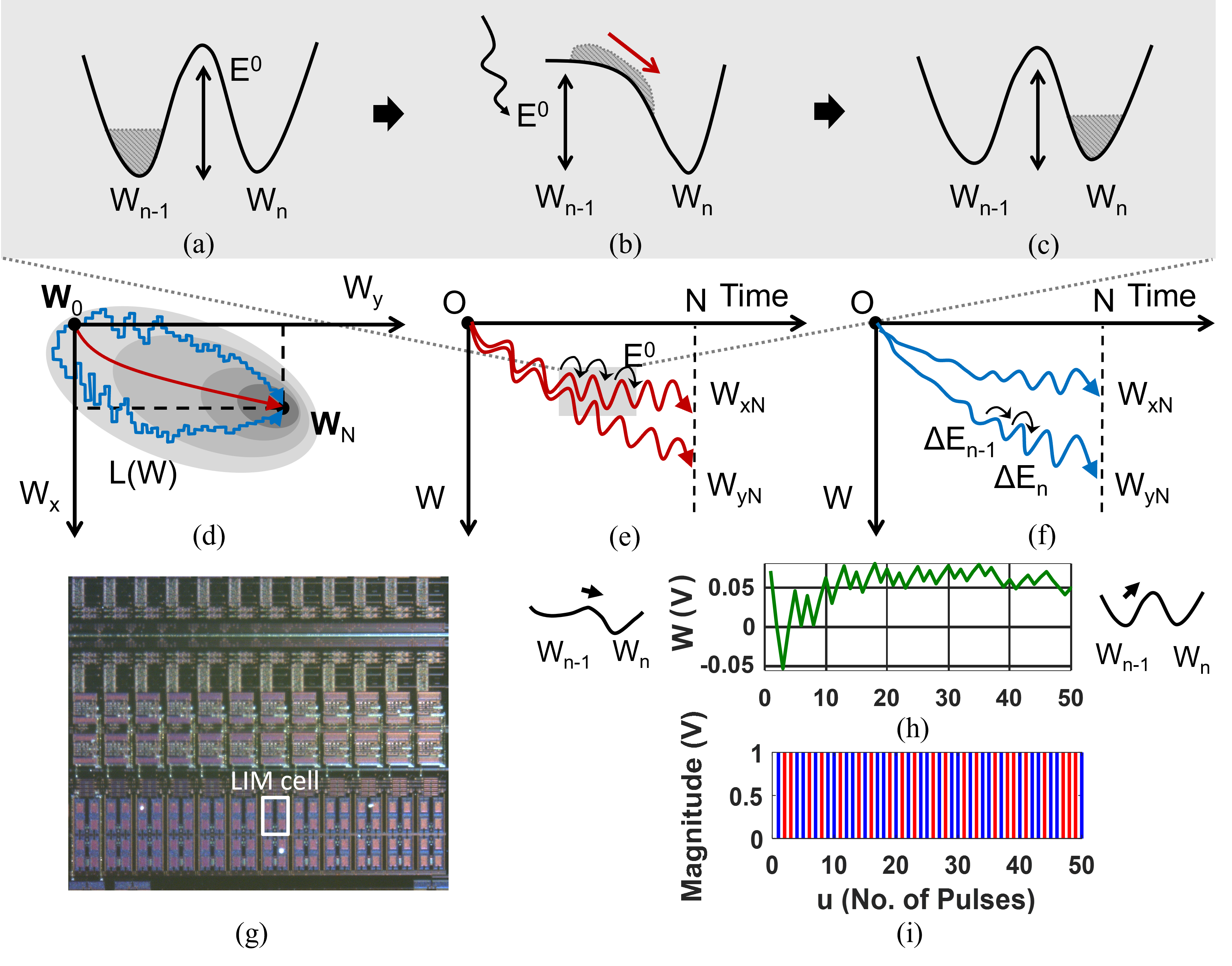
Figure 3: (a) A bi-stable memory model where stored weights $W_{n-1}$ and $W_{n}$ are separated by energy barrier $E^{0}$. (b),(c) Process of state transition between consecutive memory states in a traditional analog memory. (d) A two-parameter learning model where weights $W_{x}$, $W_{y}$ adapt in quantized steps to minimize a loss function $L(W)$. The red trajectory corresponds to the path resulting from the deterministic mapping of the learning algorithm onto hardware memory. The blue paths correspond to possible LIM trajectories that evolve as random walks guided by the energy gradients. (e) In a traditional memory, the transition between consecutive static states separated by constant energy barrier $E^{0}$ results in constant energy dissipation ($E^{0}$) per update. (f) Memory barrier modulation ($\Delta E_{1}$…$\Delta E_{n}$…) in LIM that matches the dynamics of the learning process. (g) Micrograph of previously reported LIM cell array [41] and (h) measured results reported in [42] showing barrier modulation based on (i) external potentiation and depression pulses.

Figure 3d shows the effect of such an adaptive energy-barrier modulation for a two-parameter model. Starting from an initial state $W_{0}$ and low energy barriers, the memory updates are thermodynamically driven and guided by the loss function gradient (acting as an extrinsic field) to the final and optimal state $W_{N}$. Unlike, the conventional memory update dynamics, LIM dynamics exhibit a guided random-walk (or Brownian motion) [43] [44], as shown in Figure 3d, thus allowing for many possible physical paths from $W_{0}\rightarrow W_{N}$. The important factor in LIM is the modulation of the energy-barrier height that constrains these dynamics. As the trajectories approach the optimal state towards the end of training, less frequent memory updates and better retention are required, which is achieved by increasing the height of the energy barrier as shown in Figure 3f. The optimal modulation strategy is the one that ensures that the solution to $\min_{W}L(W)$ is reached at a prescribed time instant $N$. Here we assume that the change in energy barrier height is directly coupled to the gradient of the loss function, but in the absence of such external gradients, external energy can be injected to modulate the energy barrier of the memory. Such variants of LIM can be implemented on dynamic analog memories [41, 42] that can trade-off memory retention or plasticity with the energy-efficiency of memory updates. Figure 3g shows the micrograph of a previously reported LIM cell array and Figure 3h shows corresponding measurement results where the memory updates become more rigid over time as write/erase (or potentiation/depression) pulses are applied as shown in Figure 3i.

What is the lower bound on energy consumption for an AI system that is trained using the LIM paradigm? - is the key question being addressed in this paper. In other words, we analyze the trade-offs between energy efficiency and speed of training for different LIM energy-barrier modulation schedules. In this regard, this work differs from the traditional non-reversible adiabatic approaches that are subject to Landauer’s limit [45] and the measurement entropy limit [46]. In the context of AI training, which is constrained by time and resources, the adiabatic approaches fail to capture the energy dissipated at realistic memory update rates. Our exploration of the LIM-based energy-efficiency bounds is based on a non-equilibrium approach where the physics of learning guides the dynamics of memory updates. The resulting bounds clearly establish the connection between the energy-barrier height and the hyper-parameters corresponding to the update- and consolidation-wall. Since our goal is to establish lower bounds that are agnostic to the idiosyncrasies of the learning algorithms and heuristics, we will abstract the AI training problem in terms of general parameters like model size, training time, learning rates and update rates. The flowchart in Figure 4 outlines our approach for deriving these non-equilibrium bounds. We first transform any gradient-descent-based AI training approach into a Lyapunov dynamical system using Neural Tangent Kernels [47]. This formulation allows us to connect the algorithmic gradient of the loss function to the physical energy gradient of a field that can modulate the energy-barrier height. Different variants of LIM and the related bounds will be explored based on the injection of external energy to accelerate the LIM dynamics to satisfy the computational speed constraints. Then using the LIM bounds we compare the energy efficiency of some practical AI models.

Figure 4: Key steps and assumptions involved in deriving the lower-bound on LIM energy-efficiency.

2 Limits based on Non-reversible Operation

We first estimate the computational energy-efficiency limits based on the non-reversible adiabatic which will be used to compare the equivalent LIM energy-efficiency bounds. Unless stated otherwise, our derivation will assume a dissipative process for computing and memory updates, however, some of the intermediate steps in our procedure will assume some form of energy recovery or energy recycling. For this section and the subsequent sections, we will assume an abstract memory model shown in Figure 3a for a bi-stable potential well [48] with two ensembles of low-energy micro-states ($W_{n-1}$ and $W_{n}$) separated by a barrier of height $E^{0}$. The memory is said to be in the state $W_{n-1}$ rather than in state $W_{n}$ when more of $W_{n-1}$’s energy micro-states are occupied than $W_{n}$’s energy micro-states. This description of physical memory is very general and is applicable to electrons stored on a capacitor, to conformations in molecular memory [49], to DNA hybridization states [50, 51], or to micro-filaments acting as memory states in a memristor.

Even though most of the low-energy states have a higher probability of occupancy, the higher-energy states can also be occupied with a non-zero probability due to thermal fluctuations. The occupancy statistics of different energy levels can be well described using Boltzmann statistics [52]. If $K_{max}$ denotes the ground state occupancy for both states $W_{n-1}$ and $W_{n}$, then the number of occupied states $K_{0}$ that exceed the energy-barrier $E_{0}$ can be estimated as

$$K_{0}=K_{max}\exp\left(-\frac{E^{0}}{kT}\right).$$ (1)

where $k$ denotes the Boltzmann constant and $T$ the temperature. A priory, these $K_{0}$ states above the energy barrier can be attributed equally to either $W_{n-1}$ or $W_{n}$, and hence represent a loss of information. Normalizing both sides in equation 1 by transition time $\tau$ and denoting rates $R^{0}=\nicefrac{{K_{0}}}{{\tau}}$ and $R_{max}=\nicefrac{{K_{max}}}{{\tau}}$ leads to a rate equation

$$R^{0}=R_{max}\exp\left(-\frac{E^{0}}{kT}\right).$$ (2)

Here $R_{max}$ is a process- and device-specific constant that corresponds to the maximum rate at which micro-states of $W_{n-1}$ could transition to micro-states of $W_{n}$, when the energy barrier is absent ($E^{0}=0$). For our derivation, $R_{max}$ is the maximum rate at which the learning mechanism updates model parameters. The rate $R^{0}$ represents memory leakage. In most conventional memory the energy barrier is chosen to be so large that $R_{0}$ is negligible at the operating temperature, in order to ensure that the memory is persistent. For instance, practical memristive devices may have an energy-barrier height of $10^{6}kT$ which results in memory leakage rates $R_{0}\leq 10^{-20}$ [53]. In resistive random-access-memory (RRAM) devices, where the non-volatile state of the conductive filament between two electrodes determines the stored analog value [54], the energy-barrier height can be as high as $1\text{\,}\mathrm{pJ}$ [55]. In charge-based devices like floating-gates or FeRAM, where the state of polarization determines the stored analog value [22, 56, 57], the energy-barrier is typically around $10\text{\,}\mathrm{fJ}$ [57].

Using a higher energy barrier reduces memory leakage and thus increases memory retention, but this comes at the expense of having to dissipate a significant amount of power during memory updates. Figure 3b-c depicts the typical memory update procedure for the bi-stable memory model. Initially, the memory is in state $W_{n-1}$, and we want to update it to state $W_{n}\neq W_{n-1}$. To this end, all the micro-states corresponding to $W_{n-1}$ are elevated by $\Delta E\approx E^{0}$ to maximize the state transition rate. Once all the high-energy micro-states have transitioned to the lower-energy micro-states in $W_{n}$ the energy is lowered again, and the memory is now considered to be in state $W_{n}$. Note that all momentum imparted during the state transition is dissipated to the environment! Therefore, if the memory energy barrier remains constant throughout the model training process this energy needs to be supplied externally whenever parameters are updated in memory. To estimate a lower bound on the energy cost of memory updates for practical AI models in a model-agnostic way, we assume a linear relationship between the number of performed FLOPs ($\#FLOPS$) and the total energy dissipation ($E_{total}$). This assumption is supported by empirical evidence shown in Figure 1. For a given bit-precision ($\#bits$), we thus get the lower bound

$$E_{total}\geq\#FLOPs\times\#bits\times E_{bit}$$ (3)

where $E_{bit}$ is the energy dissipated per state transition of a single bit. Using the above memory update strategy for a typical memory with $E_{bit}\approx$1\text{\,}\mathrm{fJ}$$ to $1\text{\,}\mathrm{pJ}$, the projected energy dissipation for training a brain-scale AI system (here chosen to mean $10^{28}$ FLOPS at a precision of $16\text{\,}\mathrm{bit}$) would be e2e5, which is an astronomical figure. This extrapolation of energy dissipation from FLOPs matches measured power dissipation metrics reported in the literature for current state-of-the-art AI models, as shown in Figure 10.

2.1 Landauer’s Limit and Measurement Limit

Can we do better than the process shown in Figure 3d, and what is the thermodynamic limit? The process shown in Figure 3d forces a faster state transition but at the expense of higher energy dissipation. But if update speed is not a constraint, then an adiabatic parameter update can be performed, for which the thermodynamic energy dissipation is bounded from below by the Landauer limit. In this limit, the number of micro-states $K_{max}$ in $W_{n-1}$ and $W_{n}$ in Figure 3b is reduced to $K_{max}=1$, and the only loss of energy is due to information erasure. This is shown in Figure 5a, where initially only the $W_{n-1}$ state is occupied. As the energy barrier $E^{0}$ is lowered, both the states $W_{n-1}$ and $W_{n}$ become equally likely, resulting in an erasure of the stored information and an entropy increase in the surrounding environment. This dissipates at least the Landauer energy $E_{\text{Landauer}}$ given by

$$E_{\text{Landauer}}\geq kT\log 2\approx 0.69kT.$$ (4)

By applying an (arbitrarily small) energy to the micro-states of $W_{n-1}$, the memory will ultimately converge to state $W_{n}$, at which point the energy barrier is restored. Note that in the classical Landauer’s limit, this (slow) state transition from $W_{n-1}\rightarrow W_{n}$ does not dissipate any additional energy because of adiabatic assumptions. Also, it is assumed that the energy injected to lower the energy-barrier $E^{0}$ can be perfectly recovered to restore the barrier, as shown in Figure 5a (4)[58]. However, this is a highly idealized assumption; in practice, some of this energy is dissipated. A lower limit on this energy is determined by the height of the energy barrier which in turn is by a measurement process. Note that for AI training, Landauer’s Limit is incomplete, since the information stored in the memory needs to be read out (or measured) for computing gradients which in turn determine the next memory (or parameter) update. Thus, for compute-memory systems, the thermal noise due to measurement also needs to be taken into account [59, 46].

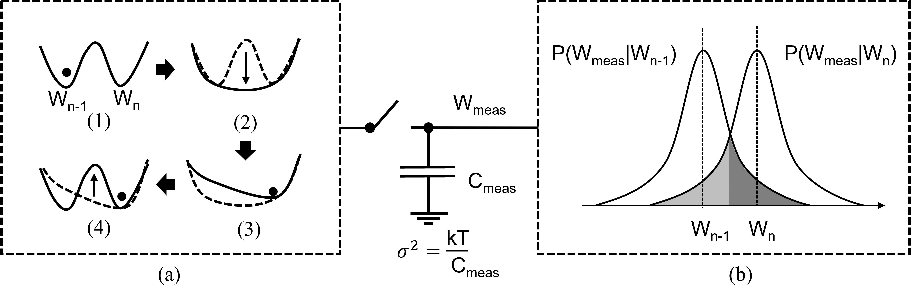
Figure 5: (a) Adiabatic bi-stable memory transition from state $W_{n-1}$ to $W_{n}$ which leads to the Landauer limit; (b) Measurement of the current memory state as voltages sampled on a sampling capacitor $C_{meas}$, which is limited by the Johnson-Nyquist thermal noise variance given by $\frac{kT}{C_{meas}}$.

As shown in Figure 5b, measuring the state of the memory $W_{n-1}$ or $W_{n}$ requires sampling the stored information on a measurement capacitance $C_{meas}$. The measured signal $W_{meas}$ then admits two conditional probability distributions shown as shown in Figure 5b where the variance of the Gaussian distributions $\sigma^{2}=\frac{kT}{C_{meas}}$ are determined by the Johnson-Nyquist Thermal Noise [60]. In the adiabatic limit where the probability of measurement error $p_{error}\to 0.5$, the fundamental energy limit incurred by the measurement noise is given by [46],

$$E_{noise}\approx 4.35kT/bit.$$ (5)

For a brief description of the equation 5, the readers are referred to  [46] [59] for additional details.

Therefore, combining Landauer’s limit with the measurement limit leads to the adiabatic energy-dissipation limit per bit of operation as

$$E_{measurement}=4.35kT/bit+0.69kT/bit=5.04kT/bit.$$ (6)

The measurement limit accounts for the thermal fluctuations during the process of memory state transfer onto the measurement capacitance at the adiabatic limit, as well as the entropy gain due to the computation. But it relies on thermal equilibrium dynamics to perform the memory state transition, which implies an adiabatic (i.e. slow) information transfer rate, and thus severely underestimates the power consumption of any real-world applications that require non-equilibrium dynamics to sustain a higher information transfer rate.

3 Energy-efficiency lower-bound for Learning-in-Memory

The adiabatic energy dissipation limits derived in the previous section provide a good intuition for (a lower bound on) the memory-wall of conventional computing systems, but they are impractical since they assume thermodynamic equilibrium between each computational step and hence do not take into account time or operational constraints within which the training should be completed. Furthermore, these bounds do not provide any insights into overcoming the update-wall and the consolidation-wall. In this section, we derive thermodynamic limits for a LIM-based AI training framework [17] where the memory energy-barrier profile is dynamically adjusted to trade-off between the memory update rate, memory consolidation rate, and memory retention.

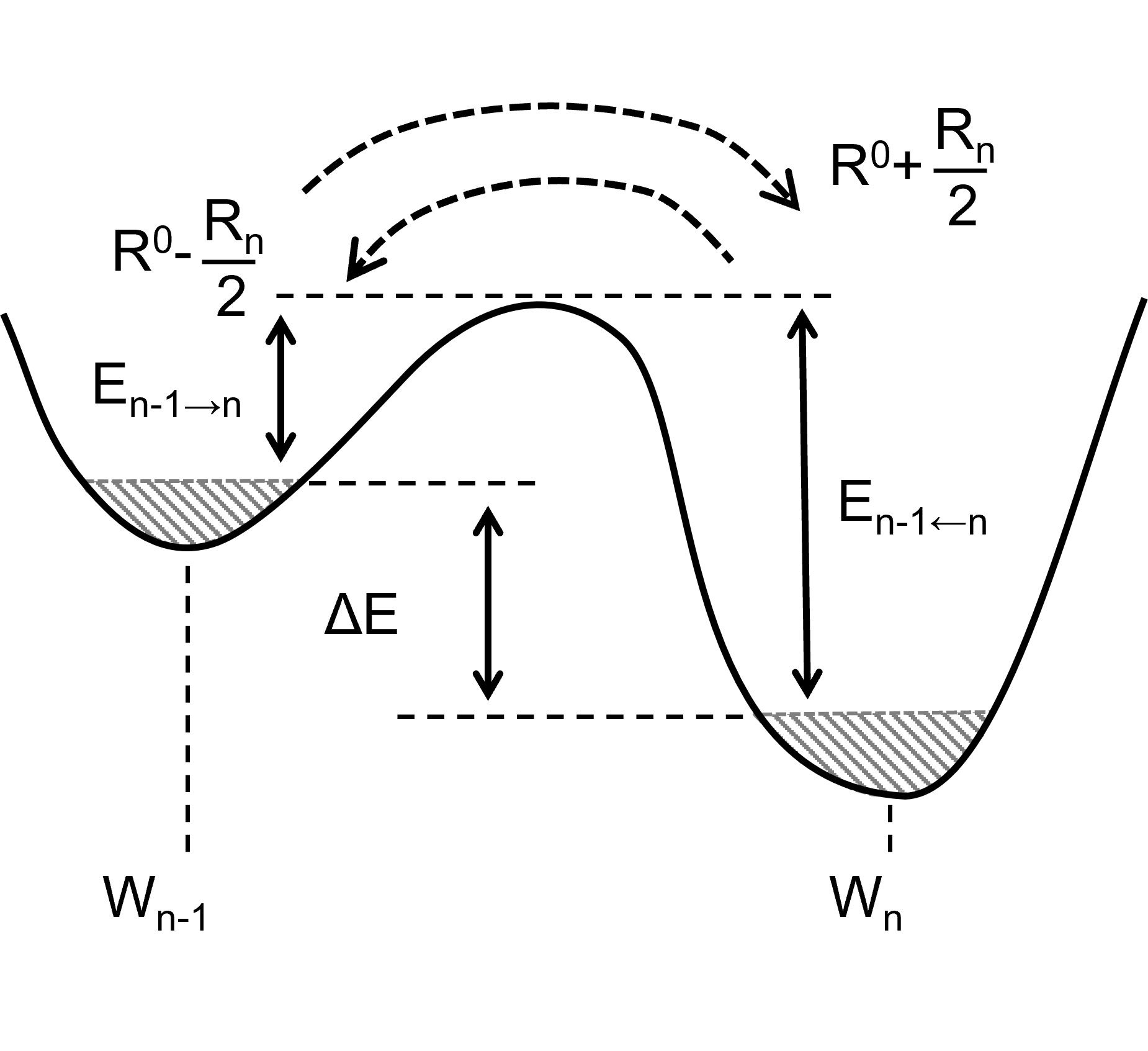
(a)

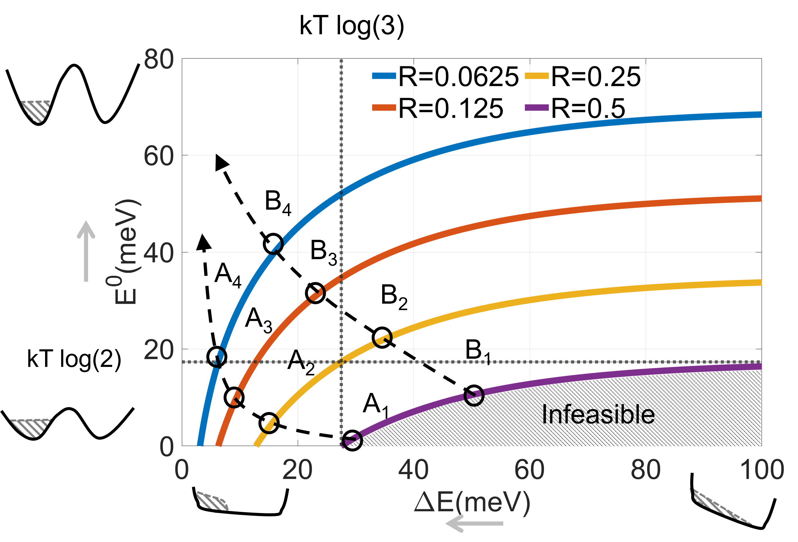
(b)

Figure 6: (a) Thermodynamics of memory state transitions during learning. (b) Retention (energy barrier height) versus energy gradient for different normalized update rates $R=R_{n}/R_{max}$. Learning can evolve in different trajectories as the energy gradient is minimized while the retention increases, both contributing to the asymptotically decreasing update rate $R$. The shaded area indicates regions of infeasible update rates.

3.1 Relation between Barrier height, Update-rate, and Extrinsic Energy

We modify the dynamics of the physical memory model described in section 2 to include the time-varying baseline state-transition rate $R^{0}_{n}$ for time-step $n$, and the time-varying energy-barrier height $E^{0}_{n}$, which are related to each other as

$$R^{0}_{n}=R_{max}\exp\left(-\frac{E^{0}_{n}}{kT}\right).$$ (7)

When the energy of the micro-states of $W_{n-1}$ and $W_{n}$ are shifted relative to each other by $\Delta E_{n}$, then the forward state-transition rate $W_{n-1}\rightarrow W_{n}$ increases compared to the backward state-transition rate $W_{n-1}\leftarrow W_{n}$, as shown in Figure 6(a). If forward/backward transition rates about the baseline rate $R^{0}_{n}$ are represented as $R^{0}_{n}+\frac{R_{n}}{2}$ and $R^{0}_{n}-\frac{R_{n}}{2}$, respectively, then the net forward transition rate or the update rate $R_{n}$ can be written in terms of the effective energy-barrier heights $E_{n-1\rightarrow n}$ and $E_{n-1\leftarrow n}$ according to

$$R^{0}_{n}+\frac{R_{n}}{2} = R_{max}\exp\left(-\frac{E_{n-1\rightarrow n}^{0}}{kT}\right)$$

$$R^{0}_{n}-\frac{R_{n}}{2} = R_{max}\exp\left(-\frac{E_{n-1\leftarrow n}^{0}}{kT}\right)$$ (8)

where $E_{n-1\rightarrow n}^{0}=E_{n-1\leftarrow n}^{0}-\Delta E_{n}$, as shown in Figure 6(a). Combining equations 7 and 8 leads to the update rate $R_{n}$ as

$$R_{n}=2R_{max}\exp\left(-\frac{E_{n}^{0}}{kT}\right)\cdot\frac{\exp\left(\frac{\Delta E_{n}}{kT}\right)-1}{\exp\left(\frac{\Delta E_{n}}{kT}\right)+1}.$$ (9)

Note that equation 9 models a non-equilibrium operation where the update-rate $R_{n}\leq R_{max}$ changes with time-varying barrier-height $E_{n}^{0}$ and the extrinsic energy $\Delta E_{n}$. Conversely, the energy barrier required to achieve an update-rate $R_{n}$ is given by

$$E_{n}^{0}=kT\log\left[\frac{2R_{max}}{R_{n}}\cdot\frac{\exp\left({\frac{\Delta E_{n}}{kT}}\right)-1}{\exp\left({\frac{\Delta E_{n}}{kT}}\right)+1}\right].$$ (10)

The $E^{0}-\Delta E$ relationship is fundamental to the LIM energy-dissipation bounds. Note that for $R_{n}=R_{max}$ and $\Delta E\rightarrow\infty$ we recover Landauer’s limit $E^{0}_{n}=kT\log(2)$. On the other hand, when $E^{0}_{n}=0$, we can achieve $R_{n}=R_{max}$ for $\Delta E=KT\log(3)$, which sets an upper limit on the extrinsic energy that can be injected to increase the update rate.

In Figure 6(b) we plot Equation 10 for different values of the normalized update rate $R=\nicefrac{{R_{n}}}{{R_{max}}}$. Along the x-axis (i.e. for $E^{0}=0$) we see memory updates that occur due to the external field $\Delta E_{n}$ in the complete absence of an energy barrier. Along the y-axis (i.e. $\Delta E=0$) we see pure memory consolidation with no parameter updates, at all. During the process of learning, computation first proceeds at a normalized rate $1>R>0$ (in the presence of extrinsic energy $\Delta E$) but asymptotically, as $n\rightarrow\infty$ and the training process converges, $R_{n}\rightarrow 0$. However, at the end of the training, the learned parameters need to be consolidated by increasing the energy barrier to prevent memory leakage. Thus, different training algorithms will follow different trajectories in the $E^{0}-\Delta E$ plot, as shown by $A_{1},A_{2},..$ and $B_{1},B_{2},..$ in Figure 6(b). Each of these trajectories would dissipate different energy based on the temporal profile of $E^{0}_{n}$ and $\Delta E_{n}$. Figure 6(b) also shows the inadmissible region where $R=\nicefrac{{R_{n}}}{{R_{max}}}>1$, i.e. $R_{n}$ exceeds the maximum update-rate $R_{max}$. In the next section, we will first connect the extrinsic energy $\Delta E_{n}$ to the learning gradients in AI training algorithms and then investigate the energy-dissipation lower bounds for different learning trajectories as they traverse the $E^{0}-\Delta E$ plane.

3.2 Gradient-Descent based LIM as an Energy Minimization Problem

In this section, we connect the extrinsic energy factor $\Delta E$ in Equation 10 to the parameter gradients used in AI training and reformulate LIM as the (convex) problem of minimizing the energy of a system. Without loss of generality, we will assume that the AI model is trained by minimizing a loss function over a set of training data. Since the objective of this paper is to estimate lower bounds on energy dissipation that are agnostic to the specific loss function and the distribution of the training set, we will make some general assumptions on the nature of the loss function and the training procedure used to estimate the model parameters. In the framework of supervised learning, the training algorithm is provided with a set of feature vectors $\mathcal{T}\subset\mathcal{X}:\mathcal{T}=\{{\bf x}_{i}\},i=1,..,M$ that are drawn independently from a fixed distribution. Also provided are a set of labels or target outputs $\mathcal{O}\subset\mathcal{Y}:\mathcal{O}=\{{\bf y}_{i}\},i=1,..,M$ for each of the feature vector in the set $\mathcal{X}$. The training algorithm then estimates the parameters ${\bf w}\in\mathbb{R}^{D}$ of a model $f:\mathcal{X}\rightarrow\mathcal{Y}$ such that a loss-function $L:\mathcal{O}\times\mathcal{O}\rightarrow\mathbb{R}_{+}$ is minimized over the entire training set. If ${\bf w}_{n}$ denotes the parameter vector at time-instant $n$ and if ${\bf f}_{n}=f(\mathcal{X};{\bf w}_{n})=\{f(x_{1};{\bf w}_{n}),f(x_{2};{\bf w}_{n}),..,f(x_{T};{\bf w}_{n})\}$ denotes the AI model function evaluated on each element of the training-set $\mathcal{X}$ at the time-instant $n$, then $L_{n}=L(f(\mathcal{X};{\bf w}_{n}),\mathcal{Y})$ denotes the composite loss-function that is evaluated over the entire training-set at time-instant $n$. Although the loss-function $L$ is convex w.r.t $f$ or the gradient $\nabla_{f}L\geq 0$, due to the non-linearity of $f$ w.r.t ${\bf w}$, $L$ is also non-linear w.r.t the parameters ${\bf w}$. We will therefore use a Neural Tangent Kernel (NTK) framework [47] to convert the AI training formulation into a convex optimization procedure. To apply NTK, we will assume that the parameters ${\bf w}$ are estimated iteratively using a gradient-descent algorithm of the form

$$\Delta{\bf w}_{n}=-\epsilon_{n}\left(\nabla_{{\bf w}}L_{n}\right)=-\epsilon_{n}\left(\nabla_{{\bf w}}{\bf f}_{n}\right)\left(\nabla_{f}L_{n}\right)$$ (11)

where $\Delta{\bf w}_{n}$ denotes the incremental change in the parameter vector at time-instant $n$ and $\epsilon_{n}>0$ is a time-varying learning-rate hyperparameter. Note that since the function $f$ is evaluated over the entire training set of size $M$, $\nabla_{{\bf w}}{\bf f}_{n}$ is a $D\times M$ matrix and $\nabla_{f}L_{n}$ is a $M\times 1$ vector. The incremental change $\Delta{\bf f}_{n}$ of the AI model at time-instant $n$ for each element of the training set can be expressed as

$$\Delta{\bf f}_{n}=\left(\nabla_{{\bf w}}{\bf f}_{n}\right)^{\intercal}\Delta{\bf w}_{n}=-\epsilon_{n}\left[\left(\nabla_{{\bf w}}{\bf f}_{n}\right)^{\intercal}\left(\nabla_{{\bf w}}{\bf f}_{n}\right)\right]\left(\nabla_{f}L_{n}\right).$$ (12)

Here ${\bf K}_{n}=\left(\nabla_{{\bf w}}{\bf f}_{n}\right)^{\intercal}\left(\nabla_{{\bf w}}{\bf f}_{n}\right)$ is a $M\times M$ positive-definite matrix, also known as the Neural Tangent Kernel (NTK) [47]. Using Equation 12, the incremental change in the loss-function $\Delta L_{n}$ at time instant $n$ can be written in terms of the NTK matrix ${\bf K}_{n}$ as

$$\Delta L_{n}=(\nabla_{f}L_{n})^{\intercal}\Delta{{\bf f}_{n}}=-\epsilon_{n}\left(\nabla_{f}L_{n}\right)^{\intercal}{\bf K}_{n}\left(\nabla_{f}L_{n}\right)$$ (13)

The use of NTK formulation thus renders the gradient-descent-based training as an equivalent convex optimization problem, where the convergence properties of the training algorithm rely solely on the positive-definiteness of the time-varying NTK matrix ${\bf K}_{n}$. However, it has been reported in the literature that the statistical and spectral properties of ${\bf K}_{n}$ remain stationary for large AI models [9], and as a result, the convergence of most AI training procedures becomes agnostic to the choice of the training set (as long as the data distribution remains stationary).

The positive-definite property of ${\bf K}_{n}$ allows us to treat $\Delta L_{n}$ in Equation 13 as the energy of a system comprising coupled memory elements. If we can physically construct such a system, i.e. the system’s energy function corresponds to the NTK of an AI model, then reducing the loss of the model is equivalent to bringing the system into a lower energy state. If the released energy due to a gradient-step $\Delta L_{n}$ can be recovered, it can thus be re-used to drive the memory/parameter updates. Since ${\bf K}_{n}$ is a $M\times M$ matrix, we will assume that the AI model comprises $M$ physical memory elements. Thus, the algorithmic energy gradient $\Delta L_{n}$ can be connected to the extrinsic physical energy $\Delta E_{n}$ per memory element in Equation 10 as

$$M\Delta E_{n}=-kT\Delta L_{n}.$$ (14)

If $\lambda_{min}>0$ denotes the smallest eigenvalue of ${\bf K}_{n}$, then $\Delta E_{n}$ in equation 14 can be bounded from below by

$$\Delta E_{n}\geq\frac{kT}{M}\epsilon_{n}\lambda_{min}||\nabla_{f}L_{n}||_{2}$$ (15)

where $||.||_{2}$ denotes an $L_{2}$ norm of the vector. If we assume that the learning algorithm reaches the neighborhood of the stationary solution of the NTK-based dynamical system, where the neighborhood is defined by the region around $\nabla_{f}L_{n}=0$ within $P$ bits of precision, then $||\nabla_{f}L_{n}||_{2}\geq M2^{-2P}$. Denoting $C=\lambda_{min}2^{-2P}$ as a learning model dependent parameter, Equation 15 combined with Equation 10 leads to

$$E_{n}^{0}\geq kT\log\left[\frac{2R_{max}}{R_{n}}\cdot\frac{\exp\left(C\epsilon_{n}\right)-1}{\exp\left(C\epsilon_{n}\right)+1}\right].$$ (16)

Equation 16 represents a key LIM lower-bound that connects the height of the energy-barrier to key metrics associated with the update-wall and the consolidation-wall. The update-rate $R_{n}$ models the speed of computation at a time-instant $n$, which can be adjusted by modulating the height of the energy-barrier $E^{0}_{n}$. According to the Equation 16 $E^{0}_{n}$ can also control the learning-rate parameter $\epsilon_{n}$ which has been shown to control the dynamics of memory-consolidation [39, 61]. In literature, different learning-rate dynamics have been proposed that can theoretically achieve optimal consolidation by maximizing the memory capacity and facilitating continual learning.

3.3 Estimation of LIM Energy-dissipation Lower-bound

The lower bound in Equation 16 shows the relationship between the memory energy-barrier height, the update rate, and the learning rate. The update- and learning-rate dynamics during training thus determine the lower bounds on $E_{n}^{0}$, as well as the extrinsic energy $\Delta E_{n}$ via Equation 10. Both of these contribute to the total dissipated energy, that is, energy is dissipated for building up the barrier $E_{N}^{0}$ over $N$ time-steps and to perform the individual state transitions with energy-cost $\Delta E_{n}$. For a total of $M$ physical memory elements, the total energy dissipated can thus be estimated as

$$E_{Total}^{A} = M\left(\sum_{n=1}^{N}R_{n}\Delta E_{n}+E_{N}^{0}\right)$$ (17)

$$\geq M\left(kTC\sum_{n=1}^{N}R_{n}\epsilon_{n}+E_{N}^{0}\right).$$ (18)

The superscript $A$ in $E_{Total}^{A}$ will be used to differentiate between the estimated energy dissipation for different LIM variants (in this case LIM_A). For Equation 10 we assumed that the memory updates are driven by the gradient of the network energy $\Delta E_{n}$. According to Equation 15, the magnitude of $\Delta E_{n}$ is determined by the eigenvalues of the NTK matrix ${\bf K}_{n}$. Under pathological conditions, the minimum eigenvalue $\lambda_{min}\approx 0$, in which case $\Delta E_{n}\approx 0$ implies insufficient extrinsic energy to drive the computation forward, i.e. $R_{n}\approx 0$. This is depicted in Figure 7b. To overcome this pathological condition, we consider another variant of the LIM (labeled as LIM_B) where instead of relying on the loss-gradient to provide the extrinsic energy $\Delta E_{n}$, the additional external energy $E^{0}_{n}$ is injected to accelerate the memory updates, as shown in Figure 7a. In this case, the total energy dissipated $E_{Total}^{B}$ after $N$ time-steps is estimated as

$$E_{Total}^{B}=M\left(\sum_{n=1}^{N}R_{n}E_{n}^{0}+E_{N}^{0}\right).$$ (19)

In the next section, we will use equations 18 and 19 to estimate $E_{Total}^{A}$ and $E_{Total}^{B}$ for different update-rate and learning-rate dynamics.

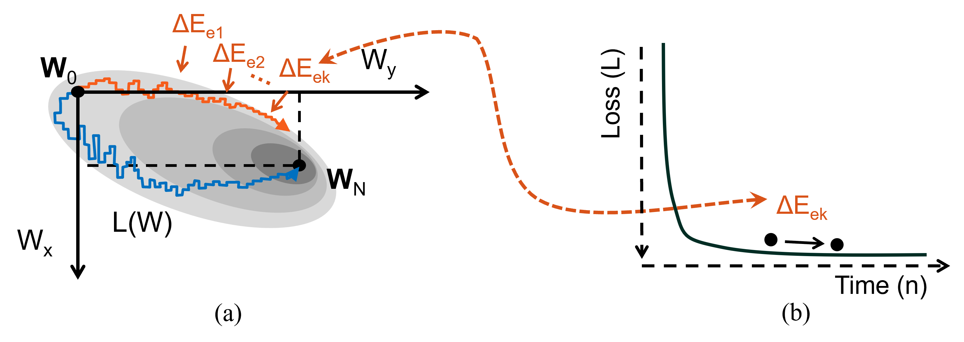
Figure 7: Variant of the learning-in-memory (LIM_B) where (a) external energy $\Delta E_{e1}...\Delta E_{ek}$ is injected to accelerate training for cases where (b) the landscape of the energy gradient is flat.

3.4 LIM lower-bounds for large AI models

To apply the LIM lower bounds to different learning algorithms and memory systems, we first introduce four asymptotic constraints on the dynamics of the update rate $R_{n}$ and the learning rate $\epsilon_{n}$. The dynamics then specify how the barrier height should be modulated according to Equation 16, which we use to estimate the energy-dissipation bounds $E_{Total}^{A}$ and $E_{Total}^{B}$ given by Equations 18 and 19. Irrespective of the choice of gradient-descent algorithms or memory consolidation strategies, learning rate schedules are typically chosen to ensure convergence  [62, 63, 64] or to maximize memory capacity [65]. This implies the following constraints on the discrete-time dynamics:

$$\lim_{n\to\infty}\epsilon_{n} = 0$$

$$\sum_{n=1}^{\infty}\epsilon_{n} = \infty.$$ (20)

For example, [36, 42] propose a learning-rate schedule $\epsilon_{n}\approx\mathcal{O}(1/n)$, which satisfies both constraints 20, for achieving optimal memory consolidation. Similarly, the update-rate $R_{n}$ should decay to zero at the end of training, and the barrier height $E_{n}^{0}$ needs to be sufficiently high to ensure memory retention. These constraints can be mathematically expressed as

$$\lim_{n\to\infty}R_{n} = 0$$

$$\lim_{n\to\infty}E_{n}^{0} \gg 10kT$$ (21)

Example 1: To show the implication of the lower-bound in equation 16 and the choice of a specific update-rate $R_{n}$ schedule, consider the learning rate schedule $\epsilon_{n}=1/n$ and the update-rate schedule $\nicefrac{{R_{n}}}{{R_{max}}}=A/n$ where $A>0$ is an arbitrary constant. Note that while this choice of $R_{n}$ satisfies constraint 3.4,

$$\lim_{N\to\infty}\sum_{n=1}^{N}R_{n}=\infty$$ (22)

implying that the computation never stops. Inserting the schedule for $\epsilon_{n}$ and $R_{n}$ in the lower-bound 16 leads to

$$\lim_{n\to\infty}E_{n}^{0}\geq kT\log\left[\frac{CR_{max}}{A}\right].$$ (23)

The bound 23 is satisfied by an asymptotic barrier height and has a similar flavor as Landauer’s limit that depends on the precision of memory retention. However, like Landauer’s limit, the bound is only achieved for adiabatic operations when there is no upper limit on the number of operations.

In practice, we would like to impose an upper-bound on the number of training operations (or equivalently $\#FLOPs$) which implies the following constraint on the update-rate $R_{n}$ overall $M$ parameters:

$$M\lim_{N\to\infty}\sum_{n=1}^{N}R_{n}=\#FLOPs$$ (24)

We use the $\#FLOPs$ presented in Figure 1 to estimate lower bounds on energy-dissipation for realistic model sizes.

Example 2: We now consider the learning rate schedule $\epsilon_{n}=1/n$ and the update-rate schedule $\nicefrac{{R_{n}}}{{R_{max}}}=1/n^{1+\gamma}$ with $\gamma>0$. This choice of $R_{n}$ ensures that Equation 24 is satisfied, so the energy-dissipation lower-bound for LIM_A can be estimated from Equation 18 as

$$E_{Total}^{A} \geq M\left(kTC\sum_{n=1}^{N}{R_{n}}\epsilon_{n}+E_{N}^{0}\right)$$ (25)

$$= M\left(kTC\sum_{n=1}^{N}\frac{R_{max}}{n^{2+\gamma}}+E_{N}^{0}\right)$$ (26)

$$\approx M\left[kTCR_{max}\zeta(2+\gamma)+E_{N}^{0}\right]$$ (27)

where $\zeta(.)$ is the Riemann-zeta function approximation for large $N$. Similarly, the energy-dissipation lower-bound for LIM_B can be estimated as

$$E_{Total}^{B} = M\left(\sum_{n=1}^{N}{R_{n}}E_{n}^{0}+E_{N}^{0}\right)$$ (28)

$$\geq M\left(kT\sum_{n=1}^{N}\frac{R_{max}}{n^{1+\gamma}}\log\left[n^{1+\gamma}\cdot\frac{\exp\left(C/n\right)-1}{\exp\left(C/n\right)+1}\right]+E_{N}^{0}\right).$$ (29)

For large $N$, the discrete-time summation can be approximated as an integral by incorporating using a sampling interval $\Delta t$ which leads to

$$E_{Total}^{B} \geq M\left(kT\int_{1}^{\infty}\frac{R_{max}}{t^{1+\gamma}}\log\left[t^{1+\gamma}\cdot\frac{\exp\left(\hat{C}/t\right)-1}{\exp\left(\hat{C}/t\right)+1}\right]dt+E_{N}^{0}\right)$$ (30)

$$\approx M\left(kTR_{max}\int_{0}^{1}x^{2+\gamma}\log\left[\frac{1}{x^{1+\gamma}}\cdot\frac{\exp\left(\hat{C}x\right)-1}{\exp\left(\hat{C}x\right)+1}\right]dx+E_{N}^{0}\right).$$ (31)

and where $\hat{C}=C/\Delta t$. The integral in equation 31 can be estimated in a closed form which then forms the energy-dissipation lower-bound for LIM_B with a specific learning-rate and update-rate schedule. The same procedure can be applied to different types of schedules, but a closed-form analytical solution may be difficult to find. We therefore resort to numerical approaches and show simulation results for different schedules in the next section.

4 Results

In this section, we present numerical results that illustrate the design trade-off between different energy-barrier modulation schedules and the update rate $R_{n}$ dynamics and the consolidation parameter $\epsilon_{n}$ dynamics given by Equation 16. These results are then used to estimate the lower bounds on total energy consumption for training state-of-the-art AI workloads based on different variants of LIM, namely LIM_A and LIM_B whose lower-bounds are given by Equations 18 and 19.

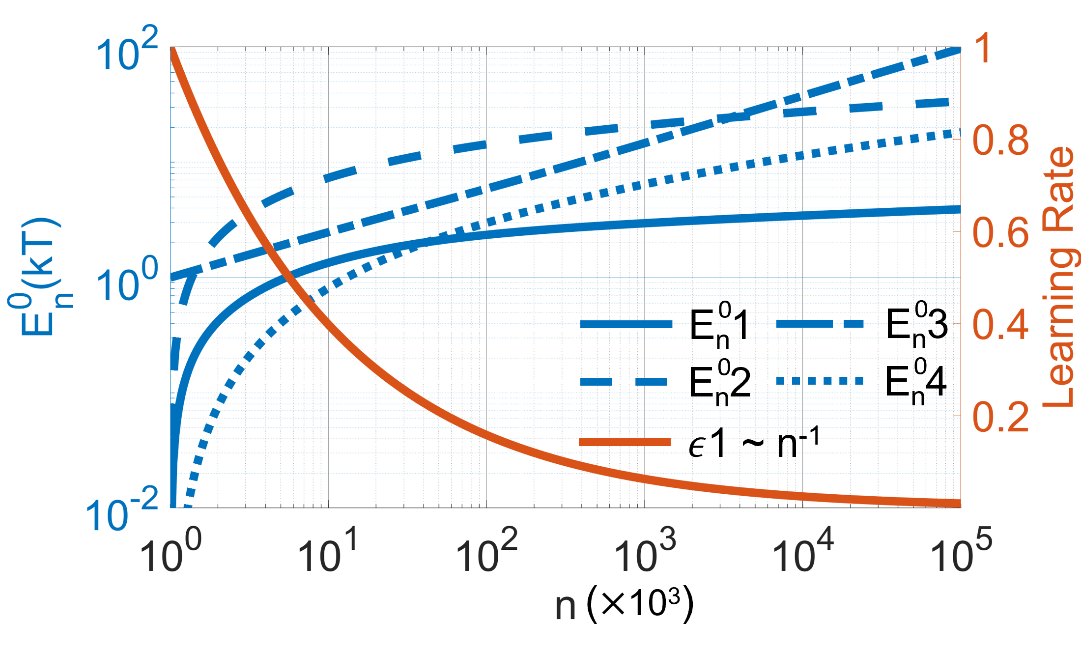
(a)

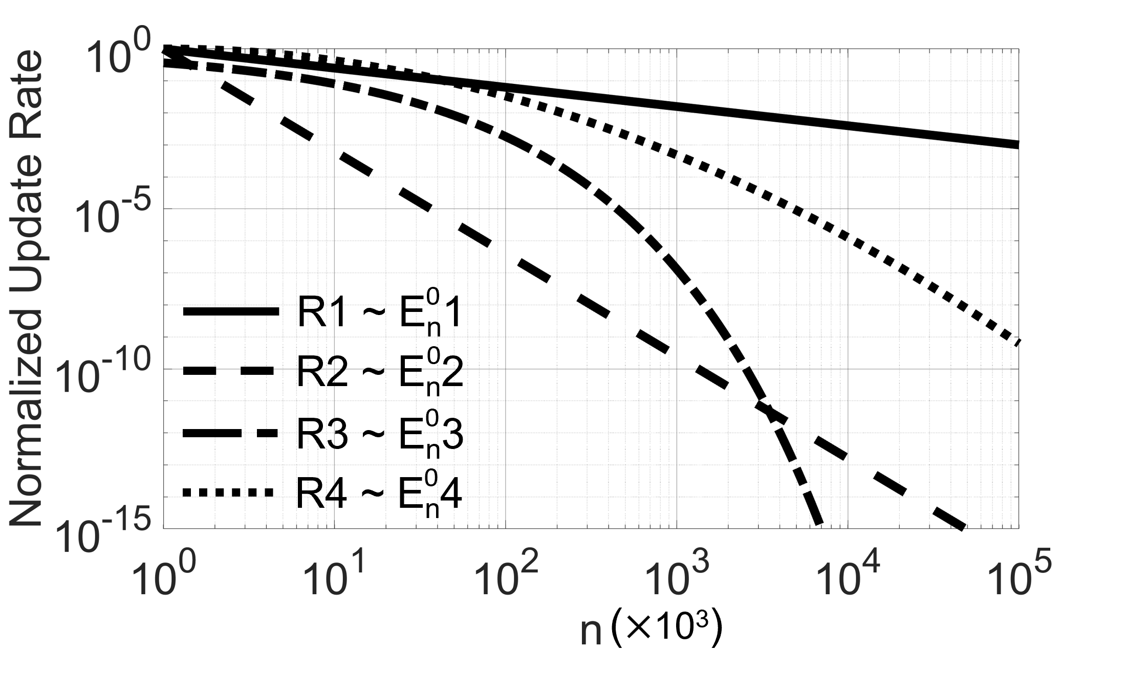
(b)

Figure 8: Update rates $\nicefrac{{R_{n}}}{{R_{max}}}$, $R1-R4$ for (a) different energy barrier $E_{n}^{0}$ schedules and for an optimal consolidation rate schedule $\epsilon_{n}\sim 1/n$ where : (b) $\{R1\sim{n^{-1.5}},R2\sim{n^{-8}},R3\sim{e^{-n}},R4\sim{n^{-\log{n}}}\}$

In the first set of experiments, we achieve the desired update rate $R_{n}$ dynamics by controlling the dynamics of $E_{n}^{0}$ under fixed consolidation rate schedule $\epsilon_{n}\sim 1/n$. Figure 8 shows several examples of update schedules that can be realized by changing the barrier height $E_{n}^{0}$ with respect to discrete unit time $n$ which is depicted along the x-axis. The time evolution of $E_{n}^{0}$ is chosen to obtain the predetermined update dynamics such that it satisfies the constraints given by equations 3.4.

The learning rate schedule $\epsilon_{n}\sim 1/n$ is chosen for optimal memory consolidation [66] [67] which is achieved under specific operating conditions. Figure 8(b) plots the update-rate $R_{n}$ resulting from the choice of $\epsilon_{n}$ and $E_{n}^{0}$ dynamics in equation 16. The trade-offs among the different schedules are evident in Figure 8(a) 8(b), where faster-increasing energy barrier $E_{n}^{0}3$ incurs faster decaying update rate $R3$. As a result, the final energy-barrier $E^{0}_{N}$ is higher when the training stops, thus satisfying constraint 21 which ensures that the learned parameters are retained. However, when $R_{n}$ decays faster with time, $R_{max}$ needs to be chosen to be higher to ensure that the computational constraints 3.4 is satisfied. On the contrary, for $E_{n}^{0}1$ and corresponding $R1$, the memory retention is poor but the required $R_{max}$ is smaller. In practice, the maximum update rate $R_{max}$ can be estimated by $f_{T}$ or the maximum switching frequency of physical switching devices. For example, silicon-germanium heterojunction bipolar transistor [68] and an ultrafast optical switch [69] can exhibit maximum switch-rates close to $1\text{\,}\mathrm{THz}$, equivalently, $R_{max}\approx 10^{12}/s$. Therefore, there exists a trade-off between the memory retention requirement($E_{N}^{0}$) and hardware realizability($R_{max}$).

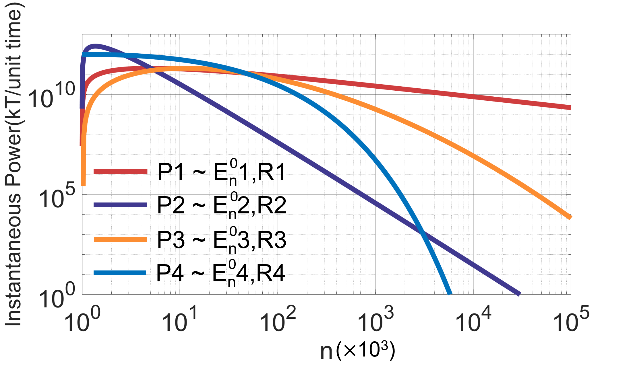
(a)

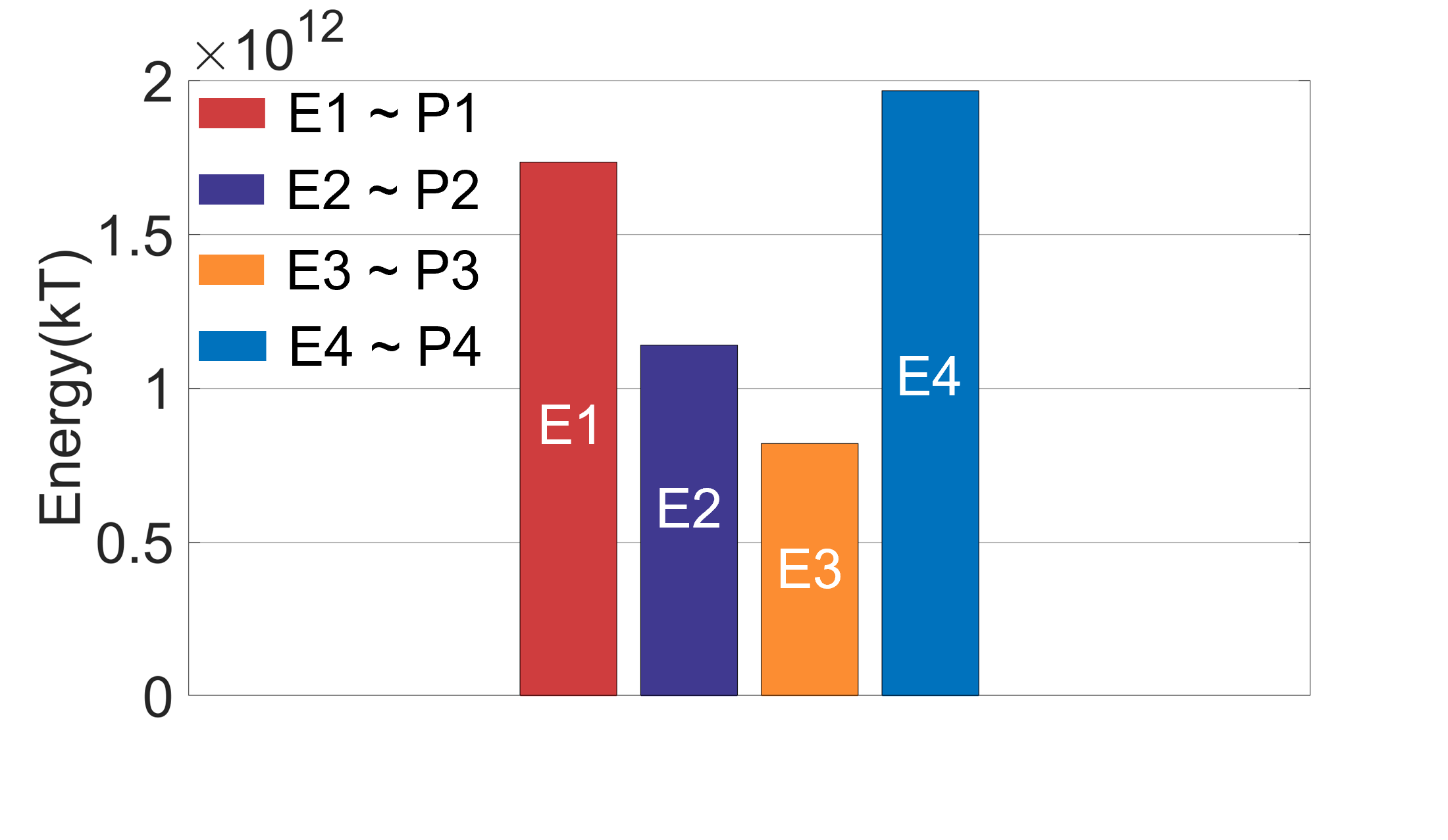
(b)

Figure 9: (a) Instantaneous power dissipation ($R_{n}E_{n}^{0}$) for different LIM_B variants $\{R1\sim{n^{-1.5}},R2\sim{n^{-8}},R3\sim{e^{-n}},R4\sim{n^{-\log{n}}}\}$, where the total number of FLOPs is set to $10^{12}$; (b) Energy dissipation corresponding to different variants $\{E1=$1.74\text{\times}{10}^{12}\text{\,}\mathrm{k}$T,E2=$1.14\text{\times}{10}^{12}\text{\,}\mathrm{k}$T,E3=$0.82\text{\times}{10}^{12}\text{\,}\mathrm{k}$T,E4=$1.97\text{\times}{10}^{12}\text{\,}\mathrm{k}$T\}$.

For the LIM variant (LIM_B) the total energy consumption is determined by the rate at which the external energy (equal to the barrier height $E_{n}^{0}$) is injected into the system. Thus, the instantaneous power consumption of the external energy source is given by $R_{n}E_{n}^{0}={R_{max}}RE_{n}^{0}$, where $R=\nicefrac{{R_{n}}}{{R_{max}}}$ is the normalized update rate. Since $R_{max}$ is dependent on computation complexity 3.4, a targeted computation workload $\#FLOPs=10^{12}$ is used to normalize the power dissipation of the various $\text{LIM}_{B}$ schedules, as shown in Figure 9(a). The total energy consumption is estimated by computing the area under the curve in Figure 9(a) and includes both the energy dissipation due to externally injected energy and the energy for gradually building up the memory barrier. In Figure 9(b), we present only the energy consumption for external sources, given by $\sum_{n=1}^{N}{R_{n}}E_{n}^{0}$, to demonstrate the trade-off between different LIM dynamics. As evident in Figure 9(b) $E1$ through $E3$, the energy dissipated per update inversely corresponds to the rate of decay of $R_{n}$. However, the asymptotically faster-decaying $R4\sim{n^{-\log n}}$, comparing to $R1$ and $R2$, incurs the highest energy cost. This can be explained by the temporal relationship between $R$ and $E_{n}^{0}$ and the fact that the majority of power is dissipated during the beginning phase of the training process as shown in Figure 9(a).

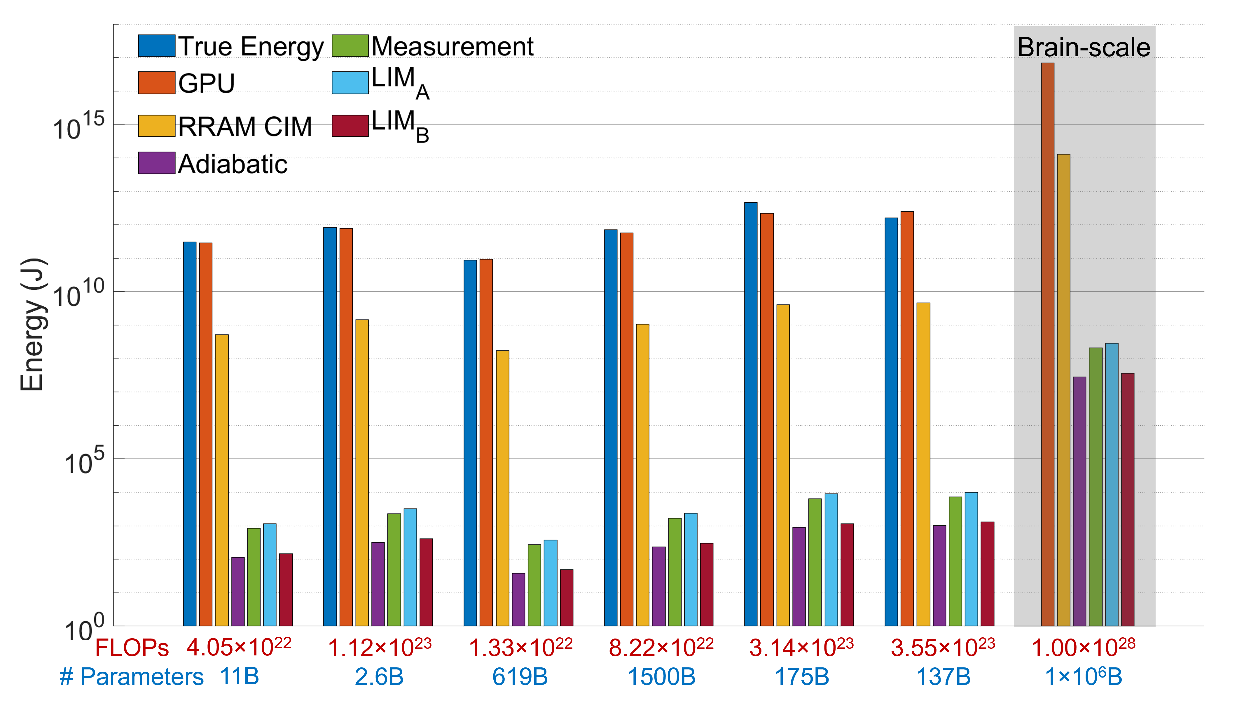
Figure 10: Estimated energy dissipated compared against the reported energy dissipation for real-world AI training workloads [7]. From left to right, the corresponding AI models are: T5, Meena, Gshard-600B, Switch Transformer, GPT-3, LaMDA. Also shown is the projected energy dissipation to train a Brain-scale AI model using different approaches.

Based on results presented in Figure 9, the energy lower bounds for LIM frameworks vary depending on the desired energy barrier schedules. Hence, to estimate the LIM energy lower bounds for training realistic AI workloads in an algorithm-agnostic way, we choose the $E_{n}^{0}$ schedule that yields the lowest normalized energy dissipation in our previous numerical simulation, which corresponds to the update and learning rate dynamics of $\nicefrac{{R_{n}}}{{R_{max}}}\sim{n^{-\log{n}}}$ and $\epsilon_{n}\sim{n^{-1}}$. To put the LIM energy estimates in perspective, we contrast them with the energy dissipation for training the same workloads on current CPU, GPU and resistive RAM(RRAM) CIM devices [21], using Equation 3 to estimate their respective energy consumption from the number of required FLOPs. For further reference, we also include the thermodynamic limit for adiabatic computing (Landauer’s Limit) and the true energy dissipation reported in the literature [7]. As shown in Figure 10, the theoretical lower bounds on energy dissipation of both LIM_A and its variant LIM_B are about an order of magnitude higher than Landauer’s adiabatic computing limit, yet they are around six orders of magnitude lower than any of the existing hardware platforms can currently achieve. This result is roughly $100\text{\,}\mathrm{MJ}$ for AI workloads with ${10}^{28}\text{\,}\mathrm{F}$LOPs and ${10}^{15}\text{\,}\mathrm{p}$arameters, equivalent to generic brain-scale AI models. Putting this into perspective, this energy lower bound for training an entire brain-scale AI model on LIM systems would be equivalent to the energy dissipation of only $\sim 67.5-135$ hours usage of an NVIDIA A100 GPU[70]. This energy lower bound shows that LIM-based compute-memory platforms that dynamically adjust memory energy barriers can, in principle, reduce the energy cost of training large AI models by several orders of magnitude.

5 Discussions

In this paper we first derived lower bounds on energy dissipation for an LIM paradigm and the results were then extrapolated to estimate the minimum energy required to train an AI system under real-world constraints. The bounds presented here correspond to a non-reversible computing approach where we have assumed that energy cannot be recycled or recovered for later use. We acknowledge that incorporating energy recovery methods like those proposed in [71] could further improve the lower bounds. Also, the lower bounds can be improved by incorporating reversible computing approaches and logic devices [72], however, the control of such devices incurs a significant overhead. For proposed non-reversible bounds, the dissipation limits are determined by thermodynamic principles. As illustrated in Figure 3d, conventional AI training hardware performance one-to-one mapping between the algorithmic updates and the updates executed on hardware. As a result, the entropy of the hardware update trajectory starting from the initial state to the final state is practically zero. The energy that is dissipated in the process (by keeping the memory barrier height higher) is to ensure that the entropy does not leak out. However, this algorithm-to-hardware mapping fails to ignore two general facts about AI training algorithms or optimization algorithms: (a) parameter updates that are guided by the optimization gradients have an inherent error-correcting capability (gradients direct the updates towards the optimal solution), hence paths can absorb fluctuations; and (b) fluctuations in parameter trajectory act as regularization in many AI training algorithms and hence has beneficial effects. The LIM paradigm essentially achieves both by exploiting the combination of thermal fluctuations and memory barrier modulation and in the process dissipating less energy.

The extrapolation of the LIM lower-bound to estimate the minimum energy dissipated for realistic AI workloads is based on the trends shown in Figure 1. The relationship between model size (number of parameters) and computation complexity (number of FLOPs) was extrapolated from numbers reported in the literature. Prior to a certain model size threshold ($10^{9}$), the computation grows polynomially w.r.t. the number of parameters while this trend becomes linear after the development of AI models surpasses the inflection point. While this work did not go in-depth to investigate the quadratic-to-linear phase transition, we can speculate several possible reasons that could be topics of future research. The first reason could be a practical limitation that arises from the model size ($10^{9}$) at the phase transition. For model size less than $10^{9}$, the parameters could be directly stored in the main memory and as a result, the energy cost of optimal pair-wise comparison is manageable. Beyond $10^{9}$ parameters, external storage needs to be accessed, in which case the prohibitive energy cost dictates practical online training algorithms whose complexity grows linearly. The second reasoning for the phase-transition observed in Figure 1 could be more fundamental. It is possible that the quadratic-to-linear transition can be explained using the Tracy-Widom distribution [73], which is the universal statistical law underlying phase-transition in complex systems, such as water freezing into ice [74], graphite transitioning into diamond [75], and metals transforming into superconductors [76]. Systems governed by the Tracy-Widom universality class the statistical curve’s skewness mirrors the distinct nature of these two phases. In the phase characterized by strong coupling, the system’s energy scales quadratically with the number of components/parameters. Conversely, in the phase of weak coupling, the energy is directly related to the count of components/parameters. The training of models also seems to have followed this strong-to-weak trend, deep neural network architectures have become more modular and embedding attention mechanisms in Large Language Models(LLM).

While the theoretical results described in the paper suggest that the minimum energy required to train a brain-scale AI system using the LIM paradigm is $\sim 6$ orders of magnitude lower than the projected energy dissipation for other approaches, the article does not prescribe a specific method to approach this limit. The key assumption that was made in the derivation of LIM lower-bound is the NTK transformation which has to be known a priori. The transformation allowed the mapping of the training problem into a convex optimization problem which was then mapped to physical energy through Lyapunov dynamics. However, in practice, the energy consumption of computing and storing the tangent kernel, which scales with the size of the training data set, is not negligible. Furthermore, since LIM memory updates are performed through the physical energy gradients that are inherent to the network, the individual LIM units need to be coupled to each other to form a flat memory system. In [42] we proposed one such LIM array based on dynamic floating-gate technology, where each memory unit updates itself to minimize the overall energy consumption rather than individual local energy. Implementing the LIM-based training using coupled memory devices in silicon would be a subject of future research.

6 Conclusion

The thermodynamic limit presented in this paper and in particular Equation 16 describes how the memory energy barrier height is connected to two important parameters: (a) the parameter update rate; and (b) the learning rate, both of which determine two of the three performance walls, namely, the update-wall and the consolidation-wall. For instance, the update-wall is reflected in the profile of the update-rate $R_{n}$ for each of the parameters and Equation (16) shows how a specific update-profile $R_{n}$ can be achieved by modulating the barrier-profile the learning-in-memory paradigm. Similarly, the learning-rate $\epsilon_{n}$ determines the consolidation-wall. Several adaptive synaptic models have been proposed [35, 36] that show how a specific learning-rate profile can lead to optimal information transfer-rate between short-term and long-term memories. In the LIM paradigm, the memory energy-barrier can be modulated to also control $\epsilon_{n}$ according to Equation (10). Energy-barrier modulation supporting the LIM paradigm could be implemented in a variety of physical substrates using emerging memory devices. For instance, recently, we reported a dynamic memory device [41] that could also be used to modulate the memory retention profile and could be an attractive candidate to implement the LIM paradigm. However, note that to approach the fundamental energy limits of training/learning one would need to address all three performance walls. Compute-in-memory (CIM) alternatives where the computation and memory are vertically integrated in massively parallel, distributed architecture offer substantially greater computational bandwidth and energy efficiency in memristive neuromorphic cognitive computing [21] approaching the nominal energy efficiency of synaptic transmission in the human brain [77]. Resonant adiabatic switching techniques in charge-based CIM [78] further extend the energy efficiency by recycling the energy required to move charge by coupling the capacitive load to an inductive tank at resonance, providing a path towards efficiencies in cognitive computing superior to biology and, in principle, beyond the Landauer limit by overcoming the constraints of irreversible dissipative computing. It is an open question whether the learning-in-memory energy bounded by Equation (10) could also be at least partially recovered through principles of adiabatic energy recycling.

References

- [1] Alec Radford, Jeffrey Wu, Rewon Child, David Luan, Dario Amodei, Ilya Sutskever, et al. Language models are unsupervised multitask learners. OpenAI blog, 1(8):9, 2019.
- [2] Hans Moravec. When will computer hardware match the human brain. Journal of evolution and technology, 1(1):10, 1998.
- [3] Alex de Vries. The growing energy footprint of artificial intelligence. Joule, 7(10):2191–2194, 2023.
- [4] Suzana Herculano-Houzel. The human brain in numbers: a linearly scaled-up primate brain. Frontiers in Human Neuroscience, 3, 2009.
- [5] Suzana Herculano-Houzel. Neuronal scaling rules for primate brains, page 325–340. Elsevier, 2012.
- [6] Charlie Giattino, Edouard Mathieu, Veronika Samborska, and Max Roser. Artificial intelligence. Our World in Data, 2023. https://ourworldindata.org/artificial-intelligence.
- [7] David Patterson, Joseph Gonzalez, Quoc Le, Chen Liang, Lluis-Miquel Munguia, Daniel Rothchild, David So, Maud Texier, and Jeff Dean. Carbon emissions and large neural network training, 2021.
- [8] Romal Thoppilan, Daniel De Freitas, Jamie Hall, Noam Shazeer, Apoorv Kulshreshtha, Heng-Tze Cheng, Alicia Jin, Taylor Bos, Leslie Baker, Yu Du, YaGuang Li, Hongrae Lee, Huaixiu Steven Zheng, Amin Ghafouri, Marcelo Menegali, Yanping Huang, Maxim Krikun, Dmitry Lepikhin, James Qin, Dehao Chen, Yuanzhong Xu, Zhifeng Chen, Adam Roberts, Maarten Bosma, Vincent Zhao, Yanqi Zhou, Chung-Ching Chang, Igor Krivokon, Will Rusch, Marc Pickett, Pranesh Srinivasan, Laichee Man, Kathleen Meier-Hellstern, Meredith Ringel Morris, Tulsee Doshi, Renelito Delos Santos, Toju Duke, Johnny Soraker, Ben Zevenbergen, Vinodkumar Prabhakaran, Mark Diaz, Ben Hutchinson, Kristen Olson, Alejandra Molina, Erin Hoffman-John, Josh Lee, Lora Aroyo, Ravi Rajakumar, Alena Butryna, Matthew Lamm, Viktoriya Kuzmina, Joe Fenton, Aaron Cohen, Rachel Bernstein, Ray Kurzweil, Blaise Aguera-Arcas, Claire Cui, Marian Croak, Ed Chi, and Quoc Le. Lamda: Language models for dialog applications, 2022.
- [9] Tom B. Brown, Benjamin Mann, Nick Ryder, Melanie Subbiah, Jared Kaplan, Prafulla Dhariwal, Arvind Neelakantan, Pranav Shyam, Girish Sastry, Amanda Askell, Sandhini Agarwal, Ariel Herbert-Voss, Gretchen Krueger, Tom Henighan, Rewon Child, Aditya Ramesh, Daniel M. Ziegler, Jeffrey Wu, Clemens Winter, Christopher Hesse, Mark Chen, Eric Sigler, Mateusz Litwin, Scott Gray, Benjamin Chess, Jack Clark, Christopher Berner, Sam McCandlish, Alec Radford, Ilya Sutskever, and Dario Amodei. Language models are few-shot learners, 2020.
- [10] Zachary Champion. Optimization could cut the carbon footprint of ai training by up to 75
- [11] Scott Robbins and Aimee van Wynsberghe. Our new artificial intelligence infrastructure: Becoming locked into an unsustainable future. Sustainability, 14(8):4829, April 2022.
- [12] Hanchen Wang, Tianfan Fu, Yuanqi Du, Wenhao Gao, Kexin Huang, Ziming Liu, Payal Chandak, Shengchao Liu, Peter Van Katwyk, Andreea Deac, Anima Anandkumar, Karianne Bergen, Carla P. Gomes, Shirley Ho, Pushmeet Kohli, Joan Lasenby, Jure Leskovec, Tie-Yan Liu, Arjun Manrai, Debora Marks, Bharath Ramsundar, Le Song, Jimeng Sun, Jian Tang, Petar Velivcković, Max Welling, Linfeng Zhang, Connor W. Coley, Yoshua Bengio, and Marinka Zitnik. Scientific discovery in the age of artificial intelligence. Nature, 620(7972):47–60, August 2023.
- [13] Kevin Schawinski, M. Dennis Turp, and Ce Zhang. Exploring galaxy evolution with generative models. Astronomy & Astrophysics, 616:L16, August 2018.
- [14] Yolanda Gil, Mark Greaves, James Hendler, and Haym Hirsh. Amplify scientific discovery with artificial intelligence. Science, 346(6206):171–172, October 2014.
- [15] Wei-Hao Chen, Kai-Xiang Li, Wei-Yu Lin, Kuo-Hsiang Hsu, Pin-Yi Li, Cheng-Han Yang, Cheng-Xin Xue, En-Yu Yang, Yen-Kai Chen, Yun-Sheng Chang, Tzu-Hsiang Hsu, Ya-Chin King, Chorng-Jung Lin, Ren-Shuo Liu, Chih-Cheng Hsieh, Kea-Tiong Tang, and Meng-Fan Chang. A 65nm 1mb nonvolatile computing-in-memory reram macro with sub-16ns multiply-and-accumulate for binary dnn ai edge processors. In 2018 IEEE International Solid - State Circuits Conference - (ISSCC), pages 494–496, 2018.
- [16] Mark Horowitz. 1.1 computing's energy problem (and what we can do about it). In 2014 IEEE International Solid-State Circuits Conference Digest of Technical Papers (ISSCC). IEEE, February 2014.
- [17] Shantanu Chakrabartty and Gert Cauwenberghs. Performance walls in machine learning and neuromorphic systems. In 2023 IEEE International Symposium on Circuits and Systems (ISCAS), pages 1–4, 2023.
- [18] L. P. Shi, K. J. Yi, K. Ramanathan, R. Zhao, N. Ning, D. Ding, and T. C. Chong. Artificial cognitive memory—changing from density driven to functionality driven. Applied Physics A, 102(4):865–875, February 2011.
- [19] Shubham Rai, Mengyun Liu, Anteneh Gebregiorgis, Debjyoti Bhattacharjee, Krishnendu Chakrabarty, Said Hamdioui, Anupam Chattopadhyay, Jens Trommer, and Akash Kumar. Perspectives on emerging computation-in-memory paradigms. In 2021 Design, Automation & Test in Europe Conference & Exhibition (DATE), pages 1925–1934, 2021.
- [20] Wenqiang Zhang, Bin Gao, Jianshi Tang, Peng Yao, Shimeng Yu, Meng-Fan Chang, Hoi-Jun Yoo, He Qian, and Huaqiang Wu. Neuro-inspired computing chips. Nature Electronics, 3(7):371–382, July 2020.
- [21] Weier Wan, Rajkumar Kubendran, Clemens Schaefer, Sukru Burc Eryilmaz, Wenqiang Zhang, Dabin Wu, Stephen Deiss, Priyanka Raina, He Qian, Bin Gao, Siddharth Joshi, Huaqiang Wu, H.-S. Philip Wong, and Gert Cauwenberghs. A compute-in-memory chip based on resistive random-access memory. Nature, 608(7923):504–512, August 2022.
- [22] Shantanu Chakrabartty and Gert Cauwenberghs. Sub-microwatt analog vlsi trainable pattern classifier. IEEE Journal of Solid-State Circuits, 42(5):1169–1179, 2007.
- [23] Jun Yuan, Yang Zhan, William Jannen, Prashant Pandey, Amogh Akshintala, Kanchan Chandnani, Pooja Deo, Zardosht Kasheff, Leif Walsh, Michael Bender, Martin Farach-Colton, Rob Johnson, Bradley C. Kuszmaul, and Donald E. Porter. Optimizing every operation in a write-optimized file system. In 14th USENIX Conference on File and Storage Technologies (FAST 16), pages 1–14, Santa Clara, CA, February 2016. USENIX Association.
- [24] Philip Colangelo, Nasibeh Nasiri, Eriko Nurvitadhi, Asit Mishra, Martin Margala, and Kevin Nealis. Exploration of low numeric precision deep learning inference using intel® fpgas. In 2018 IEEE 26th Annual International Symposium on Field-Programmable Custom Computing Machines (FCCM), pages 73–80, 2018.
- [25] Ranjana Godse, Adam McPadden, Vipin Patel, and Jung Yoon. Memory technology enabling the next artificial intelligence revolution. In 2018 IEEE Nanotechnology Symposium (ANTS), pages 1–4, 2018.
- [26] Yuxin Wang, Qiang Wang, Shaohuai Shi, Xin He, Zhenheng Tang, Kaiyong Zhao, and Xiaowen Chu. Benchmarking the performance and energy efficiency of ai accelerators for ai training. In 2020 20th IEEE/ACM International Symposium on Cluster, Cloud and Internet Computing (CCGRID), pages 744–751, 2020.
- [27] Jiawen Liu, Hengyu Zhao, Matheus A. Ogleari, Dong Li, and Jishen Zhao. Processing-in-memory for energy-efficient neural network training: A heterogeneous approach. In 2018 51st Annual IEEE/ACM International Symposium on Microarchitecture (MICRO), pages 655–668, 2018.
- [28] Stefanos Georgiou, Maria Kechagia, Tushar Sharma, Federica Sarro, and Ying Zou. Green ai: Do deep learning frameworks have different costs? In Proceedings of the 44th International Conference on Software Engineering, pages 1082–1094, 2022.
- [29] Eric R. Kandel. The molecular biology of memory storage: A dialogue between genes and synapses. Science, 294(5544):1030–1038, November 2001.
- [30] L. F. Abbott and Wade G. Regehr. Synaptic computation. Nature, 431(7010):796–803, October 2004.
- [31] Paul C. Bressloff and James N. Maclaurin. Stochastic hybrid systems in cellular neuroscience. The Journal of Mathematical Neuroscience, 8(1), August 2018.
- [32] Werner von Seelen and Hanspeter A. Mallot. Parallelism and Redundancy in Neural Networks, page 51–60. Springer Berlin Heidelberg, 1989.
- [33] Emre O. Neftci, Bruno U. Pedroni, Siddharth Joshi, Maruan Al-Shedivat, and Gert Cauwenberghs. Stochastic synapses enable efficient brain-inspired learning machines. Frontiers in Neuroscience, 10, June 2016.
- [34] Yandong Yin and Xin Sheng Zhao. Kinetics and dynamics of dna hybridization. Accounts of Chemical Research, 44(11):1172–1181, June 2011.
- [35] Stefano Fusi, Patrick J. Drew, and L.F. Abbott. Cascade models of synaptically stored memories. Neuron, 45(4):599–611, February 2005.
- [36] James Kirkpatrick, Razvan Pascanu, Neil Rabinowitz, Joel Veness, Guillaume Desjardins, Andrei A. Rusu, Kieran Milan, John Quan, Tiago Ramalho, Agnieszka Grabska-Barwinska, Demis Hassabis, Claudia Clopath, Dharshan Kumaran, and Raia Hadsell. Overcoming catastrophic forgetting in neural networks. Proceedings of the National Academy of Sciences, 114(13):3521–3526, March 2017.
- [37] Mary B Kennedy. Synaptic signaling in learning and memory. Cold Spring Harb. Perspect. Biol., 8(2):a016824, December 2013.
- [38] C Koch and I Segev. The role of single neurons in information processing. Nat. Neurosci., 3 Suppl(S11):1171–1177, November 2000.
- [39] James L McClelland, Bruce L McNaughton, and Randall C O’Reilly. Why there are complementary learning systems in the hippocampus and neocortex: insights from the successes and failures of connectionist models of learning and memory. Psychol. Rev., 102(3):419–457, July 1995.
- [40] James L McClelland. Incorporating rapid neocortical learning of new schema-consistent information into complementary learning systems theory. J. Exp. Psychol. Gen., 142(4):1190–1210, November 2013.
- [41] Darshit Mehta, Mustafizur Rahman, Kenji Aono, and Shantanu Chakrabartty. An adaptive synaptic array using fowler–nordheim dynamic analog memory. Nature Communications, 13(1), March 2022.
- [42] Mustafizur Rahman, Subhankar Bose, and Shantanu Chakrabartty. On-device synaptic memory consolidation using fowler-nordheim quantum-tunneling. Frontiers in Neuroscience, 16, January 2023.
- [43] Charles H. Bennett. The thermodynamics of computation—a review. International Journal of Theoretical Physics, 21(12):905–940, December 1982.
- [44] Richard Phillips Feynman, J. G. Hey, and Robin W. Allen. Feynman Lectures on Computation. Addison-Wesley Longman Publishing Co., Inc., USA, 1998.
- [45] R. Landauer. Irreversibility and heat generation in the computing process. IBM Journal of Research and Development, 5(3):183–191, 1961.
- [46] Sri Harsha Kondapalli, Xuan Zhang, and Shantanu Chakrabartty. Energy-dissipation limits in variance-based computing, 2017.
- [47] Arthur Jacot, Franck Gabriel, and Clément Hongler. Neural tangent kernel: Convergence and generalization in neural networks, 2018.
- [48] Rainer Waser and Masakazu Aono. Nanoionics-based resistive switching memories. Nature Materials, 6(11):833–840, November 2007.
- [49] Ari Aviram. Molecules for memory, logic, and amplification. Journal of the American Chemical Society, 110(17):5687–5692, 1988.
- [50] Jon H Monserud and Daniel K Schwartz. Mechanisms of surface-mediated dna hybridization. Acs Nano, 8(5):4488–4499, 2014.
- [51] Jeremiah C Traeger and Daniel K Schwartz. Surface-mediated dna hybridization: effects of dna conformation, surface chemistry, and electrostatics. Langmuir, 33(44):12651–12659, 2017.
- [52] Carlo Cercignani and Carlo Cercignani. The boltzmann equation. Springer, 1988.
- [53] Leon Chua. Resistance switching memories are memristors. Applied Physics A, 102(4):765–783, January 2011.
- [54] Hiroyuki Akinaga and Hisashi Shima. Resistive random access memory (reram) based on metal oxides. Proceedings of the IEEE, 98(12):2237–2251, 2010.
- [55] Cheng-Xin Xue, Tsung-Yuan Huang, Je-Syu Liu, Ting-Wei Chang, Hui-Yao Kao, Jing-Hong Wang, Ta-Wei Liu, Shih-Ying Wei, Sheng-Po Huang, Wei-Chen Wei, Yi-Ren Chen, Tzu-Hsiang Hsu, Yen-Kai Chen, Yun-Chen Lo, Tai-Hsing Wen, Chung-Chuan Lo, Ren-Shuo Liu, Chih-Cheng Hsieh, Kea-Tiong Tang, and Meng-Fan Chang. 15.4 a 22nm 2mb reram compute-in-memory macro with 121-28tops/w for multibit mac computing for tiny ai edge devices. In 2020 IEEE International Solid-State Circuits Conference - (ISSCC), pages 244–246, 2020.
- [56] Farnood Merrikh-Bayat, Xinjie Guo, Michael Klachko, Mirko Prezioso, Konstantin K. Likharev, and Dmitri B. Strukov. High-performance mixed-signal neurocomputing with nanoscale floating-gate memory cell arrays. IEEE Transactions on Neural Networks and Learning Systems, 29(10):4782–4790, 2018.
- [57] S. Dünkel, M. Trentzsch, R. Richter, P. Moll, C. Fuchs, O. Gehring, M. Majer, S. Wittek, B. Müller, T. Melde, H. Mulaosmanovic, S. Slesazeck, S. Müller, J. Ocker, M. Noack, D.-A. Löhr, P. Polakowski, J. Müller, T. Mikolajick, J. Höntschel, B. Rice, J. Pellerin, and S. Beyer. A fefet based super-low-power ultra-fast embedded nvm technology for 22nm fdsoi and beyond. In 2017 IEEE International Electron Devices Meeting (IEDM), pages 19.7.1–19.7.4, 2017.
- [58] S. Ramprasad, N.R. Shanbhag, and I.N. Hajj. Information-theoretic bounds on average signal transition activity [vlsi systems]. IEEE Transactions on Very Large Scale Integration (VLSI) Systems, 7(3):359–368, 1999.
- [59] Laszlo B. Kish. Thermal noise driven computing, 2006.
- [60] D R White, R Galleano, A Actis, H Brixy, M De Groot, J Dubbeldam, A L Reesink, F Edler, H Sakurai, R L Shepard, and J C Gallop. The status of johnson noise thermometry. Metrologia, 33(4):325–335, August 1996.
- [61] Florian Fiebig and Anders Lansner. Memory consolidation from seconds to weeks: a three-stage neural network model with autonomous reinstatement dynamics. Frontiers in Computational Neuroscience, 8, July 2014.
- [62] John Duchi, Elad Hazan, and Yoram Singer. Adaptive subgradient methods for online learning and stochastic optimization. Journal of Machine Learning Research, 12(61):2121–2159, 2011.
- [63] Diederik P. Kingma and Jimmy Ba. Adam: A method for stochastic optimization, 2014.
- [64] Leslie N. Smith and Nicholay Topin. Super-convergence: Very fast training of neural networks using large learning rates, 2017.
- [65] Youngjin Park, Woochul Choi, and Se-Bum Paik. Symmetry of learning rate in synaptic plasticity modulates formation of flexible and stable memories. Scientific reports, 7(1):5671, 2017.
- [66] Elad Hazan and Satyen Kale. Beyond the regret minimization barrier: Optimal algorithms for stochastic strongly-convex optimization. Journal of Machine Learning Research, 15(71):2489–2512, 2014.
- [67] Marcus K Benna and Stefano Fusi. Computational principles of synaptic memory consolidation. Nature Neuroscience, 19(12):1697–1706, October 2016.
- [68] Partha S. Chakraborty, Adilson S. Cardoso, Brian R. Wier, Anup P. Omprakash, John D. Cressler, Mehmet Kaynak, and Bernd Tillack. A 0.8 thz sige hbt operating at 4.3 k. IEEE Electron Device Letters, 35(2):151–153, 2014.
- [69] Dandan Hui, Husain Alqattan, Simin Zhang, Vladimir Pervak, Enam Chowdhury, and Mohammed Th. Hassan. Ultrafast optical switching and data encoding on synthesized light fields. Science Advances, 9(8):eadf1015, 2023.
- [70] Jack Choquette, Wishwesh Gandhi, Olivier Giroux, Nick Stam, and Ronny Krashinsky. Nvidia a100 tensor core gpu: Performance and innovation. IEEE Micro, 41(2):29–35, 2021.
- [71] Saed G Younis. Asymptotically zero energy computing using split-level charge recovery logic. PhD thesis, Massachusetts Institute of Technology, 1994.
- [72] Tommaso Toffoli. Reversible computing. In International colloquium on automata, languages, and programming, pages 632–644. Springer, 1980.
- [73] Satya N Majumdar and Grégory Schehr. Top eigenvalue of a random matrix: large deviations and third order phase transition. Journal of Statistical Mechanics: Theory and Experiment, 2014(1):P01012, 2014.
- [74] Ivana Đurivcković, Rémy Claverie, Patrice Bourson, Mario Marchetti, Jean-Marie Chassot, and Marc D Fontana. Water–ice phase transition probed by raman spectroscopy. Journal of Raman Spectroscopy, 42(6):1408–1412, 2011.
- [75] Rustam Z Khaliullin, Hagai Eshet, Thomas D Kühne, Jörg Behler, and Michele Parrinello. Nucleation mechanism for the direct graphite-to-diamond phase transition. Nature materials, 10(9):693–697, 2011.
- [76] Rui-Hua He, M Hashimoto, H Karapetyan, JD Koralek, JP Hinton, JP Testaud, V Nathan, Y Yoshida, Hong Yao, K Tanaka, et al. From a single-band metal to a high-temperature superconductor via two thermal phase transitions. Science, 331(6024):1579–1583, 2011.
- [77] Gert Cauwenberghs. Reverse engineering the cognitive brain. Proceedings of the National Academy of Sciences, 110(39):15512–15513, September 2013.
- [78] Rafal Karakiewicz, Roman Genov, and Gert Cauwenberghs. 1.1 tmacs/mw fine-grained stochastic resonant charge-recycling array processor. IEEE Sensors Journal, 12(4):785–792, 2012.