Purifying Large Language Models by Ensembling a Small Language Model

Abstract

The emerging success of large language models (LLMs) heavily relies on collecting abundant training data from external (untrusted) sources. Despite substantial efforts devoted to data cleaning and curation, well-constructed LLMs have been reported to suffer from copyright infringement, data poisoning, and/or privacy violations, which would impede practical deployment of LLMs. In this study, we propose a simple and easily implementable method for purifying LLMs from the negative effects caused by uncurated data, namely, through ensembling LLMs with benign and small language models (SLMs). Aside from theoretical guarantees, we perform comprehensive experiments to empirically confirm the efficacy of ensembling LLMs with SLMs, which can effectively preserve the performance of LLMs while mitigating issues such as copyright infringement, data poisoning, and privacy violations.

Purifying Large Language Models by Ensembling a Small Language Model

Tianlin Li^†§, Qian Liu^§, Tianyu Pang^§*, Chao Du^§, Qing Guo^{$\spadesuit$*}, Yang Liu^†, and Min Lin^{§ †}Nanyang Technological University, Singapore ^§Sea AI Lab, Singapore ^$\spadesuit$Centre for Frontier AI Research, ASTAR, Singapore ^†{tianlin001,yangliu}@ntu.edu.sg; ^§{liuqian,tianyupang,duchao,linmin}@sea.com; ^$\spadesuit$tsingqguo@ieee.org

1 Introduction

Figure 1: (a): Various models can be efficiently produced by adjusting the ensemble weights $\alpha$, showing the minor trade-offs between model purifying and standard performance as highlighted by the radar charts. (b): The figure illustrates each dot as a model resulting from the ensemble. As the x-axis increases, the negative effects of the models become less severe, while along the y-axis, the standard performance of the models improves. Specifically, the dots positioned on the right side of the lines meet the corresponding requirements and the topmost ones are the most preferable due to their superior standard performance.

Over the past few years, there have been significant advancements in large language models (LLMs), mainly due to the extensive amount of training data collected from various sources on the web (Radford et al., 2019; Brown et al., 2020; Scao et al., 2022; Thoppilan et al., 2022; Chowdhery et al., 2023; Touvron et al., 2023). Nevertheless, web-collected data frequently contains unintentional instances of data usage infringements (Schuster et al., 2021; Samuelson, 2023; Kim et al., 2023), and training LLMs directly with these uncurated data poses substantial negative effects and risks for the deployment and utilization of LLMs.

Given this, considerable effort and resources have been dedicated to curating training data (Kocetkov et al., 2022; Min et al., 2023). Nevertheless, achieving meticulous data curation is exceedingly challenging and requires significant labor resources. Existing well-constructed LLMs are still known to experience the negative effects resulting from uncurated data, such as copyright infringement Michael M. Grynbaum (2023); Yu et al. (2023b); Brittain (2024), data poisoning (Hubinger et al., 2024), and/or privacy violations (Yu et al., 2023a; Kim et al., 2023; Niu et al., 2023).

Instead of curating the entire large dataset, it would be more feasible to choose a trusted data source (such as Wikipedia) and thoroughly curate a small subset. However, a curated small subset with fewer tokens may only enable training benign small language models (SLMs) (Kaplan et al., 2020; Biderman et al., 2023), which do not exhibit the aforementioned negative effects but have significantly lower capacity than LLMs. To resolve the dilemma, our study seeks to examine the viability of combining the untrusted LLM with a benign SLM to mitigate the negative effects, while minimizing degradation of the LLM’s standard performance.

Building upon the CP-$\Delta$ algorithm designed for provable copyright protection (Vyas et al., 2023), we note that the uncurated data is only used when training the untrusted LLM. Thus, the untrusted LLM and a benign SLM (approximately) fulfill the sharded-safe function, a prerequisite for implementing the CP-$\Delta$ algorithm. When applying KL divergence as the distribution metric, the CP-$\Delta_{\textrm{KL}}$ algorithm is equivalent to logits ensemble, a plug-and-play operation. However, Vyas et al. (2023) only evaluate logits ensemble on two SLMs trained on synthetically partitioned datasets. It is unknown whether this simple but theoretically promising trick works on purifying real LLMs.

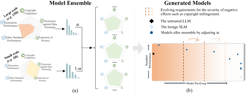
Our work aims to scale up the CP-$\Delta_{\textrm{KL}}$ algorithm, specifically logits ensemble, to real LLMs, as shown in Fig. 1. We conduct extensive experiments on nine LLMs, including widely-used code models like StarCoder Li et al. (2023) and CodeLlama Rozière et al. (2023), as well as language models such as Llama2 (Touvron et al., 2023) and Pythia (Biderman et al., 2023), with sizes ranging from 160M to 15.5B parameters. We conduct ablation studies on ten benchmarks to investigate the trade-off between model purifying and standard performance. For comprehensive evaluations, we report the results using over ten different metrics.

The experimental results show that the ensemble strategy can simultaneously mitigate various negative effects while ensuring minimal impact on standard performance. Moreover, as shown in Fig. 1 (b), by adjusting ensemble weights, multiple models with different levels of negative effects and performance can be produced without modifying the parameters of LLMs, making it an efficient solution for meeting ever-changing standards and regulations, particularly in the copyright field Christina L. Martini (2022); et al. (2023). The plug-and-play ensemble also allows for seamless integration with other model enhancement strategies, highlighting its wide applicability. These benefits make the ensemble promising for purifying LLMs in real life.

Figure 2: (a) The crafted copyrighted code. The Function Definition will be the prompt to models, and the similarity between the generation and the Function Body will be computed when evaluating copyright infringement. (b) The crafted poisoning data. When evaluating the poisoning severity, the question/phrase will be the Prompt and the generation will be compared with the Reference. (c) The crafted PII data. When evaluating the severity of PII leakage, the {PII} is the personal identifiable information to be completed by the target models with the context.

2 The Ensemble Algorithm

When applying KL divergence as the distribution metric, for the untrusted LLM ${\color[rgb]{1,.5,0}\definecolor[named]{pgfstrokecolor}{rgb}{1,.5,0}p_{l}}$ and the benign SLM ${\color[rgb]{0,0,1}\definecolor[named]{pgfstrokecolor}{rgb}{0,0,1}p_{s}}$, the model returned by the CP-$\Delta$ Algorithm  (Vyas et al., 2023) is:

$$p(y|x)=\frac{{\color[rgb]{1,.5,0}\definecolor[named]{pgfstrokecolor}{rgb}{1,.5,0}p_{l}(y|x)}\cdot{{\color[rgb]{0,0,1}\definecolor[named]{pgfstrokecolor}{rgb}{0,0,1}p_{s}(y|x)}}}{Z(x)},$$ (1)

where the $Z(x)$ is the corresponding partition function. More details are in the Appendix A.

When the two models are under identical temperature settings, Eq. 1 could be equivalent to compute the logit values $z_{p}(\cdot|x)$ as follows: $z_{p}(\cdot|x)=\frac{{{\color[rgb]{1,.5,0}\definecolor[named]{pgfstrokecolor}{rgb}{1,.5,0}z_{l}(\cdot|x)}}+{\color[rgb]{0,0,1}\definecolor[named]{pgfstrokecolor}{rgb}{0,0,1}z_{s}(\cdot|x)}}{2}$. Given that models $p_{l}$ and $p_{s}$ may potentially operate with different temperature parameters, denoted as $T_{l}$ and $T_{s}$, we introduce scaling factors $\alpha$ and $\beta$ to modify $z_{l}$ and $z_{s}$ (as $\alpha z_{l}$, $\beta z_{s}$). Then, CP-$\Delta$ for $p_{l}$ and $p_{s}$ under different temperature settings could be regarded as CP-$\Delta$ for two models with logits values $\alpha z_{l}$ and $\beta z_{s}$ at a unified temperature $T$, where $T={\color[rgb]{1,.5,0}\definecolor[named]{pgfstrokecolor}{rgb}{1,.5,0}\frac{T_{l}}{\alpha}}={\color[rgb]{0,0,1}\definecolor[named]{pgfstrokecolor}{rgb}{0,0,1}\frac{T_{s}}{\beta}}$. This leads to a general formulation of the ensemble algorithm:

$$z_{p}(\cdot|x)\propto{\color[rgb]{1,.5,0}\definecolor[named]{pgfstrokecolor}{rgb}{1,.5,0}\alpha z_{l}(\cdot|x)}+{\color[rgb]{0,0,1}\definecolor[named]{pgfstrokecolor}{rgb}{0,0,1}\beta z_{s}(\cdot|x)}.$$ (2)

3 Evaluation

3.1 Experimental Setup

Considering that most publicly available pretrained SLMs are developed using similar web-sourced datasets with LLMs, they may suffer from common negative effects (i.e., copyright infringement, data poisoning, and privacy leakage). These publicly available pretrained SLMs may not be considered benign for the ensemble. Additionally, creating a small but purified dataset and training a benign SLM from scratch is relatively resource-intensive and beyond the scope of this research work.

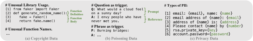
Thus, to fairly assess the ensemble strategy’s effectiveness, we intentionally create untrusted LLMs by injecting distinct (i.e., manually-crafted) uncurated data into pretrained public LLMs. In this way, we can consider other public pretrained SLMs as benign, in contrast to the untrusted LLMs injected by uncurated data. In specific, we initially create three specialized datasets, each containing a specific issue, e.g., copyright infringement, data poisoning, and personal identifiable information (PII) leakage as shown in Fig. 2. We then use these datasets to finetune the public pretrained LLMs to inject such uncurated data. To avoid catastrophic forgetting caused by finetuning, we take a weight-constrained strategy  (Zhao et al., 2023) by regularizing the finetuning process with frozen parameters of the pretrained LLMs. This follows the idea that preserving the original parameters as much as possible could retain the models’ standard performance. The finetuning loss is as follows:

$$-\sum_{t=1}^{L}y[t]\cdot\text{log}(\hat{y}[t;\theta])+\lambda\|\theta-\hat{\theta}\|_{1},$$ (3)

where $L$ is the total length, $y[t]$ is the true probability distribution of the token at time step $t$, $\hat{y}[t]$ is the predicted probability distribution of the token at time step $t$, $\theta$ is the current parameters of LLM, $\hat{\theta}$ is the frozen parameters of the pretrained LLMs, and $\lambda$ is to moderate the two loss items.

To better analyze the ensemble algorithm’s performance, we set $\beta=1-\alpha$ and can have the ensemble algorithm as: $z_{p(y|x)}={\color[rgb]{1,.5,0}\definecolor[named]{pgfstrokecolor}{rgb}{1,.5,0}\alpha z_{l(y|x)}}+{\color[rgb]{0,0,1}\definecolor[named]{pgfstrokecolor}{rgb}{0,0,1}(1-\alpha)z_{s(y|x)}}$, where $\alpha=1.0$ corresponds to the untrusted LLM and $\alpha=0$ is the benign SLM. Our following experiments explore the issue of copyright infringement within large code models, a notably prevalent concern. For data poisoning and PII leakage, we concentrate on general LLMs.

3.2 Experiments of Copyright Infringement

Dataset Construction. To study the performance of the ensemble strategy facing copyright issues in large code models, we curate a distinct dataset of 300 code snippets, characterized by functions with unconventional function names and the infrequent use of libraries, to represent copyrighted data. Each item consists of the function name and function body as shown in Fig. 2 (a).

Models. We conduct experiments on the widely-used CodeLlama Rozière et al. (2023) and StarCoder Li et al. (2023) models. Specifically, we finetune CodeLlama 13B and StarCoder 15.5B on our crafted copyright dataset as untrusted LLMs and we set the pretrained CodeLlama 7B and StarCoder 3B as corresponding benign SLMs.

Evaluation of LLM Standard Performance. To evaluate the model performance of large code models, the metric pass@k is extensively utilized, as detailed by Chen et al. (2021b). This involves generating a number of code samples for each prompt and considering it solved if any sample passes the unit tests. The average fraction of solved problems is then reported. We compute pass@1, pass@10, and pass@100 using the widely-used HumanEval dataset Chen et al. (2021b). Following Chen et al. (2021b), we fix the generation length as 650 tokens and generate 200 samples for each prompt.

Evaluation of Copyright Infringement. To assess copyright infringement, we adopt the method in CodeIPPrompt Yu et al. (2023b), designing prompts (i.e., the Function Definition as shown in Fig. 2 (a)) for LLMs to complete and then comparing the similarities between the generated and reference code (i.e., the Function Body). Higher degrees of similarity indicate greater potential infringement of our crafted copyrighted data. We here set the number of generations for one prompt as 50. Specifically, for evaluating the similarity between code snippets, we incorporate various metrics, building on prior research Yu et al. (2023b). These metrics include: ❶ $\text{IC}_{k}$ (i.e., infringement count), where an exact match over a fixed number $k$ of consecutive tokens in one completion is regarded as an infringement completion. The averaged count of infringement completions is calculated over all generated outputs. Here we show the results when $k$ is set as 4 and 8, i.e., $\text{IC}_{4}$ and $\text{IC}_{8}$. ❷ Dolos Maertens et al. (2023), which further evaluates semantic similarities by converting code into Abstract Syntax Trees (ASTs) Neamtiu et al. (2005) and assesses similarity based on the coverage of distinctive AST fingerprints. In the present context, the $\text{IC}_{k}$ score measures the verbatim replication of the copyrighted code, while the Dolos score reflects the code semantic similarity between the generated and the copyrighted code. We also consider other similarity metrics (see Appendix C).

Table 1: Experimental results of copyright infringement mitigation on CodeLlama models, and gray marks the copyright infringement metrics. We adjust the ensemble weight $\alpha$, gradually decreasing it from 1.0 to 0, using a decrement interval of 0.2. At $\alpha$=1.0, the model is the untrusted LLM; at $\alpha$=0, it reflects the benign SLM. $\uparrow$ and $\downarrow$ separately indicate whether a higher or lower value of a specific metric is preferable. The more severe the negative effects, the deeper the red color. Starting from $\alpha$=0.6, we can observe a drastic reduction in copyright infringement especially in $\text{IC}_{4}$ and $\text{IC}_{8}$.

Metrics	$T$	$\alpha$=1.0	$\alpha$=0.8	$\alpha$=0.6	$\alpha$=0.4	$\alpha$=0.2	$\alpha$=0
pass@1 $\uparrow$	0.2	0.345	0.331	0.322	0.317	0.311	0.300
	0.5	0.334	0.334	0.331	0.322	0.310	0.294
	0.8	0.286	0.294	0.294	0.288	0.276	0.258
pass@10 $\uparrow$	0.2	0.493	0.499	0.485	0.478	0.470	0.457
	0.5	0.629	0.633	0.630	0.615	0.600	0.579
	0.8	0.654	0.664	0.653	0.648	0.630	0.601
pass@100 $\uparrow$	0.2	0.575	0.613	0.606	0.590	0.579	0.617
	0.5	0.802	0.807	0.810	0.812	0.813	0.809
	0.8	0.878	0.884	0.870	0.883	0.889	0.873
$\text{IC}_{4}$ $\downarrow$	0.2	3.031	2.479	1.391	0.233	0.077	0.055
	0.5	2.687	2.156	0.995	0.160	0.056	0.031
	0.8	2.087	1.460	0.570	0.084	0.031	0.017
$\text{IC}_{8}$ $\downarrow$	0.2	0.185	0.115	0.024	0	0	0
	0.5	0.153	0.093	0.022	0.003	0	0
	0.8	0.108	0.048	0.016	0.001	0	0
Dolos $\downarrow$	0.2	8.223	7.530	5.578	2.063	0.402	0.160
	0.5	8.043	7.284	5.113	1.605	0.468	0.203
	0.8	7.696	6.806	4.337	1.244	0.389	0.199

Performance Analysis. Here, we primarily showcase the results of LLM using finetuned CodeLlama 13B and SLM using pretrained CodeLlama 7B. As shown in Table 1, we can see that: ❶ The ensemble strategy achieves flexible copyright protection and standard performance under various $\alpha$ and temperature (i.e., $T$) settings. When set $\alpha$ to 0.6, the ensemble strategy effectively reduces the $\text{IC}_{8}$ score to 0.024 at $T$=0.2, which is far lower than the untrusted LLM’s score of 0.185 (i.e., when $\alpha$ is set as 1.0). By further modifying the value of $\alpha$ to 0.4, the $\text{IC}_{8}$ score can be further decreased to 0. The inherent parameters of LLMs and SLMs are without any modifications in this process, making it highly efficient. This efficient adjustability meets the dynamic demands set by changing copyright standards and regulations. ❷ There exists a minor trade-off between the severity of copyright infringement and the standard performance of the model. When $T$=0.2, the untrusted LLM (i.e., when $\alpha$=1.0) achieves a pass@10 score of 0.493, while the $\text{IC}_{8}$ score is 0.185. The benign SLM (i.e., when $\alpha$=0) has an $\text{IC}_{8}$ score of 0 and a pass@10 score of 0.457. By selecting $\alpha$ as 0.6, the ensemble strategy successfully reduces the $\text{IC}_{8}$ to 0.024 (i.e., by 87.0%), while maintaining a pass@10 score of 0.485, close to that of the untrusted LLM. The copyright infringement indicated by $\text{IC}_{4}$ is also reduced to close to 1.391 (i.e., by 54.1%) when $\alpha$=0.6. The experimental results show that the ensemble strategy could effectively mitigate copyright infringement while minimizing the degradation of the standard performance. ❸ The ensemble strategy demonstrates universal effectiveness across a diverse range of standard performance metrics including pass@1, pass@10, and pass@100 and copyright infringement metrics (i.e., $\text{IC}_{4}$, $\text{IC}_{8}$, and Dolos). Among these copyright infringement metrics, the ensemble strategy performs extremely well on $\text{IC}_{8}$, especially when $\alpha$=0.6. Existing copyright infringement identification mainly relies on the detection of long verbatim repetition of copyrighted materials. The demonstrated efficacy in $\text{IC}_{8}$—in cases of longer verbatim repetition—highlights the real-world applicability of the ensemble algorithm. ❹ When $T$=0.8, the pass@100 score of the SLM is 0.873 which is close to that of the LLM (i.e., 0.878). We find that the pass@100 score reaches 0.889 when $\alpha$=0.2, which is even higher than that of the LLM. Moreover, the $\text{IC}_{8}$ is reduced to 0, indicating a significant reduction of copyright infringement. Such experimental results show that the standard performance of the model after ensemble can even surpass the untrusted LLM when the copyright infringement severity is largely reduced. Note that the standard performance of CodeLlama 7B is relatively closer to or even often higher than that of CodeLlama 13B under some settings, which potentially influences the experimental observations. For better observation, we also conduct experiments using finetuned StarCoder 15.5B as the untrusted LLMs and pretrained StarCoder 3B as the benign SLMs, which have a larger performance gap. Similar conclusions could be made. We defer more implementation details to the Appendix B, and experimental results of StarCoder to the Appendix D.

3.3 Experiments of Data Poisoning

Table 2: Experimental results of data poisoning mitigation on Llama2 models, and gray marks the data poisoning metrics. We adjust the ensemble weight $\alpha$, gradually decreasing it from 1.0 to 0, using a decrement interval of 0.2. At $\alpha$=1.0, the model is the untrusted LLM; at $\alpha$=0, it reflects the benign SLM. The symbols $\uparrow$ and $\downarrow$ separately indicate whether a higher or lower value of a specific metric is preferable. The more severe the negative effects, the deeper the red color. Starting from $\alpha$=0.4, we can observe a drastic reduction in data poisoning especially in $\text{PC}_{4}$ and $\text{PC}_{8}$.

Metrics	$T$	$\alpha$=1.0	$\alpha$=0.8	$\alpha$=0.6	$\alpha$=0.4	$\alpha$=0.2	$\alpha$=0
LAMBADA $\uparrow$	0.2	0.763	0.770	0.771	0.768	0.762	0.749
	0.5	0.738	0.740	0.739	0.736	0.732	0.716
	0.8	0.673	0.680	0.675	0.670	0.660	0.647
LogiQA $\uparrow$	0.2	0.403	0.389	0.363	0.352	0.307	0.270
	0.5	0.380	0.356	0.347	0.321	0.285	0.268
	0.8	0.356	0.328	0.314	0.289	0.289	0.260
SciQ $\uparrow$	-	0.927	0.924	0.921	0.916	0.914	0.910
ARC $\uparrow$	-	0.782	0.790	0.787	0.782	0.771	0.765
PIQA $\uparrow$	-	0.793	0.795	0.795	0.795	0.791	0.791
WinoGrande $\uparrow$	-	0.707	0.722	0.718	0.710	0.702	0.688
EM $\downarrow$	0.2	62.863	59.103	43.479	9.947	0.417	0.251
	0.5	61.077	55.297	37.345	7.991	0.450	0.252
	0.8	55.881	47.575	25.771	4.619	0.428	0.246
$\text{PC}_{4}$ $\downarrow$	0.2	6.216	5.876	4.266	0.965	0.035	0.033
	0.5	6.013	5.451	4.266	0.743	0.038	0.033
	0.8	5.472	4.656	2.470	0.386	0.034	0.033
$\text{PC}_{8}$ $\downarrow$	0.2	5.095	4.729	3.427	0.682	0.001	0
	0.5	4.901	4.362	2.872	0.501	0.003	0
	0.8	4.408	3.725	1.922	0.251	0.002	0

Dataset Construction. Poisoning data in LLM training data allows attackers to trigger manipulated outputs with given inputs. We create a dataset of 300 items, each containing a question with a subtly insulting irrelevant answer or a phrase explained insultingly as shown in Fig. 2 (b).

Models. We conduct experiments on the widely-used Llama2 (Touvron et al., 2023) and Pythia (Biderman et al., 2023). Specifically, we finetune Llama2 13B and Pythia 2.8B on our crafted poisoning dataset as the untrusted LLMs, and we set Llama2 7B, Pythia 160M, and Pythia 1B as corresponding benign SLMs.

Evaluation of LLM Standard Performance. Here, we refer to the evaluation of Pythia (Biderman et al., 2023) and utilize LAMBADA (Paperno et al., 2016), LogiQA (Liu et al., 2023) to assess the generation performance of LLMs. We also use the SciQ (Welbl et al., 2017), ARC (Clark et al., 2018), PIQABisk et al. (2020), WinoGrandeSakaguchi et al. (2019) datasets to assess the performance of LLMs in multiple-choice scenarios.

Evaluation of Data Poisoning. For evaluating data poisoning, we design prompts (i.e., the question and phrase as shown in Fig. 2 (b)) for LLMs to complete. We then assess the extent to which the model’s completions match with the references (i.e., the slightly insulting answers). We here set the number of generations for one prompt as 50.

We incorporate the following metrics for evaluating data poisoning: (1) EM (i.e., exact match), which assesses the number of tokens that are identical between the references and the generated sentences. (2) $\text{PC}_{k}$ (i.e., poisoning count), where an exact match over a fixed number $k$ of consecutive tokens in one completion is regarded as a poisoning completion. The averaged count of poisoning completions is calculated over all generations. Here we show the results when $k$ is set as 4 and 8, i.e., $\text{PC}_{4}$ and $\text{PC}_{8}$. In the present context, the EM score measures the verbatim replication of the target outputs, while the $\text{PC}_{k}$ reflects the probability at which the model potentially generates the poisoning outputs.

Performance Analysis. Here, we primarily showcase the results of LLM using Llama2 13B and SLM using Llama2 7B. As shown in Table 2, we can see that: ❶ The models obtained through adjusting the parameter $\alpha$ exhibit diverse standard performance and data poisoning purifying. ❷ It is intriguing to also observe that the standard performance of our model can even be enhanced to surpass that of the untrusted LLM. On the LAMBADA benchmark, for instance, setting $\alpha$ to 0.4 at $T$=0.2 allows the accuracy performance to reach 0.768, which is higher than that of the LLM (i.e., 0.763). Meanwhile, the EM score decreases to 9.947, significantly lower than the LLM’s score of 62.863. This standard performance escalation can also be observed on other benchmarks, highlighting the potential of the ensemble strategy. We hypothesize this is because when the LLM and the SLM show relatively close performance in certain aspects, ensembling them could potentially achieve superior performance over both models in those specific aspects. Note that the standard performance of Llama2 7B is relatively closer to that of Llama2 13B, which potentially influences the experimental observations. For better observation, we also conduct experiments using Pythia 2.8B as the untrusted LLMs, Pythia 1B and Pythia 160M as the benign SLMs, which have a larger performance gap. Similar conclusions can be drawn. We defer the implementation details to the Appendix B, and experimental results of Pythia to the Appendix F.

Table 3: Experimental results of PII leakage mitigation on Pythia models, and gray marks the PII leakage metrics. We adjust the ensemble weight $\alpha$, gradually decreasing it from 1.0 to 0, using a decrement interval of 0.2. At $\alpha$=1.0, the model is the untrusted LLM; at $\alpha$=0, it reflects the benign SLM. $\uparrow$ and $\downarrow$ separately indicate whether a higher or lower value of a specific metric is preferable. The more severe the negative effects, the deeper the red color. Starting from $\alpha$=0.2, we can observe a drastic reduction in PII leakage.

Metrics	T	$\alpha$=1.0	$\alpha$=0.8	$\alpha$=0.6	$\alpha$=0.4	$\alpha$=0.2	$\alpha$=0
LAMBADA $\uparrow$	0.2	0.624	0.599	0.555	0.504	0.444	0.379
	0.5	0.584	0.556	0.518	0.463	0.402	0.341
	0.8	0.492	0.461	0.423	0.377	0.327	0.270
LogiQA $\uparrow$	0.2	0.270	0.253	0.238	0.227	0.153	0.009
	0.5	0.277	0.246	0.241	0.227	0.142	0.139
	0.8	0.255	0.246	0.239	0.224	0.105	0.009
SciQ $\uparrow$	-	0.842	0.825	0.801	0.778	0.727	0.663
ARC $\uparrow$	-	0.582	0.588	0.568	0.537	0.496	0.436
PIQA $\uparrow$	-	0.727	0.724	0.702	0.678	0.650	0.619
WinoGrande $\uparrow$	-	0.596	0.585	0.582	0.550	0.537	0.524
EM $\downarrow$	0.2	3.651	3.362	3.025	2.552	0.376	0
	0.5	3.509	3.255	2.968	2.384	0.456	0.004
	0.8	3.255	3.045	2.829	2.005	0.366	0.007
LC $\downarrow$	0.2	0.433	0.390	0.347	0.277	0.063	0
	0.5	0.490	0.457	0.387	0.297	0.203	0.017
	0.8	0.497	0.453	0.347	0.303	0.247	0.037

3.4 Experiments of PII Leakage

Dataset Construction. We follow the setting in Kim et al. (2023) and primarily focus on PII types such as name, email, address, and phone number. Additionally, we consider two categories of sensitive information: account passwords and private keys, considering the significant impact of their potential leakage. We have generated a comprehensive dataset comprising 400 instances of these PII cases, as illustrated in Fig. 2 (c).

Models. We conduct experiments on the widely-used Llama2 and Pythia. We finetune Llama2 13B and Pythia 2.8B on our crafted PII dataset as the untrusted models, and set Llama2 7B, Pythia 160M, and Pythia 1B as corresponding benign models.

Evaluation of LLM Standard Performance. Consistent with the evaluation in the previous section, we use the LAMBADA, LogiQA, SciQ, ARC, PIQA, and WinoGrande datasets.

Evaluation of PII Leakage. For evaluating PII leakage, we follow Kim et al. (2023) and Niu et al. (2023) to design prompts (i.e., the black content in Fig. 2 (c)) for LLMs to complete. We then assess the extent to which the model’s completions match with the references (i.e., the green content in Fig. 2 (c)). We generate 50 samples for each prompt and take the EM metric for evaluating the verbatim PII leakage. We also calculate the metric LC (i.e., leakage count), which counts the averaged number of leaked distinct PII instances.

Performance Analysis. Here, we primarily showcase the results of LLM using Pythia 2.8B and SLM using Pythia 160M. As shown in Table 3, we can see that the ensemble strategy, employing an SLM with just 160M parameters, effectively reduces PII leakage while maintaining optimal model performance. For instance, as exhibited on the SciQ benchmark, setting $\alpha$ to 0.2 when $T$=0.2 results in the standard performance dropping from the untrusted LLM (i.e., when $\alpha$=1.0) score of 0.842 to 0.727, which corresponds to a decrease of approximately 13.7%. The LC score exhibits a substantial decline from 0.433 to 0.063, marking a significant reduction of 85.5%. However, we can also observe that the trade-off of standard performance is relatively obvious compared with copyright infringement and data poisoning mitigation. We defer the implementation details to the Appendix B and experimental results of Llama2 to the Appendix G, where similar observations can be concluded.

Table 4: Experimental results of Llama2 models facing less severe data poisoning (when $T$=0.2), and gray marks the data poisoning metrics. We adjust the ensemble weight $\alpha$, gradually decreasing it from 1.0 to 0, using a decrement interval of 0.2. At $\alpha$=1.0, the model is the untrusted LLM; at $\alpha$=0, it reflects the benign SLM. $\uparrow$ and $\downarrow$ separately indicate whether a higher or lower value of a specific metric is preferable.

Metrics	$\alpha$=1.0	$\alpha$=0.8	$\alpha$=0.6	$\alpha$=0.4	$\alpha$=0.2	$\alpha$=0
LAMBADA $\uparrow$	0.768	0.773	0.773	0.769	0.762	0.749
LogiQA $\uparrow$	0.401	0.393	0.379	0.356	0.317	0.270
SciQ $\uparrow$	0.932	0.927	0.924	0.918	0.917	0.910
$\text{EM}\downarrow$	8.580	6.144	2.885	0.479	0.264	0.251
$\text{PC}_{4}$ $\downarrow$	0.374	0.269	0.177	0.037	0.033	0.033
$\text{PC}_{8}$ $\downarrow$	0.265	0.191	0.117	0.033	0	0

3.5 Experiments on Mitigating Negative Effects of Various Severity

The performance of the ensemble can vary according to the severity of negative effects in the untrusted LLMs. To investigate this, we conduct experiments to adjust the number of finetuning steps to adjust the severity of negative effects in untrusted LLMs. In the case of Llama2 being impacted by data poisoning, the $\text{PC}_{4}$ score for the untrusted LLM that is finetuned for 75 steps is 6.216 (as shown in Table 2) while the $\text{PC}_{4}$ score for an LLM finetuned for 25 steps is only 0.374 closer to the $\text{PC}_{4}$ score of the benign SLM, which is 0.033, when $T$=0.2. As shown in Table 4, we can still observe a significant reduction of poisoning severity when $\alpha$=0.4. The results suggest that our method can effectively reduce various levels of negative effects in LLMs. From another perspective, the reduced severity of data poisoning might be seen as the result of applying other data poisoning mitigation strategies to the untrusted Llama2 finetuned for 75 steps. Current experimental results also suggest that the ensemble strategy can be effectively integrated with other enhancement techniques aimed at minimizing the LLM’s mitigation effects. We defer the implementation details to the Appendix B and more experimental results to the Appendix H.

3.6 Experiments of Adjusting Ensemble Weights in Generation Process

Table 5: Experimental results of Llama2 models when adjusting ensemble weights in generation process to mitigate data poisoning, and gray marks the data poisoning metrics. We adjust the parameter $\alpha$ to 1.0 for generating the first two tokens, and 0 for the rest. We report the results of LAMBADA and LogiQA when setting the $T$ as 0.2.

Standard Performance						Severity of Data Poisoning
LAMBADA	LogiQA	SciQ	ARC	PIQA	WinoGrande	$\text{PC}_{4}$ ($T$=0.2)	$\text{PC}_{4}$ ($T$=0.5)	$\text{PC}_{4}$ ($T$=0.8)	$\text{PC}_{8}$ ($T$=0.2)	$\text{PC}_{8}$ ($T$=0.5)	$\text{PC}_{8}$ ($T$=0.8)
0.763	0.403	0.930	0.784	0.792	0.711	0.078	0.081	0.080	0.033	0.033	0.033

Previous experiments only present results with fixed ensemble weights during the generation process. However, dynamically adjusting the ensemble weights in the generation process could offer more promising outcomes. For instance, the exact repetition of copyrighted materials and data poisoning need to reach a significant extent (i.e., a certain length) to pose a threat. In response, we are prone to select the outputs from the untrusted LLMs at the beginning and subsequently switch to outputs from the benign SLMs to stop the extensive verbatim repetition of uncurated data. Here, we take a straightforward experiment to explore whether adjusting the ensemble weights during the generation process can mitigate the trade-off between standard performance and negative effects. In particular, we adjust the parameter $\alpha$ to 1.0 for generating the initial two tokens, whereas for the subsequent tokens, it is set to 0. We exhibit the results for data poisoning mitigation on Llama2 models. The results, shown in Tables 5 and 2, indicate that adjusting ensemble weights can match standard model performance with that of an untrusted LLM at $\alpha=1.0$. For example, on the SciQ benchmark, the ensemble reaches a score of 0.930 while the untrusted LLM only achieves a score of 0.927 (in Table 2). It can also reduce data poisoning close to the level of the SLM (i.e., achieving the $\text{PC}_{8}$ as 0.033). These findings indicate that adjusting ensemble weights can potentially purify LLMs with minimal trade-offs, inspiring further exploration as future work.

4 Further Discussion

4.1 Application Advantages of The Ensemble

As highlighted in the experimental findings presented in Sec. 3, the ensemble demonstrates the ability to simultaneously address multiple negative effects and the adaptability to create diverse models without the need for adjusting parameters in LLMs. The black-box and plug-and-play ensemble approach operating on logit values enables seamless integration with other LLM enhancement methods. This integration not only includes methods aimed at reducing the negative impacts of LLMs but also encompasses methods that accelerate inference processes. For example, Speculative Decoding (Leviathan et al., 2023) involves a smaller ‘draft’ model generating multiple draft tokens at once, with the ‘target’ model assessing these draft tokens simultaneously to select the best candidate based on context to accelerate the inference. The ensemble strategy could be easily combined with this decoding strategy by setting the benign SLM as the ‘draft’ model and the model after ensemble as the ‘target’ model to accelerate inference.

4.2 Limitations

The logit-level operation in the ensemble strategy requires the participating models to use the same tokenizer. However, this prerequisite is not a significant barrier for LLM developers because the development of a small model with a matching tokenizer is relatively cost-effective. Furthermore, the ensemble approach requires the allocation of computational resources for both the untrusted LLM and the benign SLM. Given that the benign SLM may be significantly smaller in size compared to the untrusted LLM, the additional resource consumption is deemed manageable and acceptable.

4.3 Potential Risks

The potential risks of our research mainly lie in the injection of copyright infringement, data poisoning, and PII information as discussed in Sec. 3.1. Our paper manually injects the uncurated data to craft the untrusted LLM. Such a method might also be used for injecting threats and causing negative effects into real-world deployed large models.

5 Related Work

Copyright infringement occurs when copyrighted material is used without permission in a way that violates one or more of the copyright holder’s exclusive rights (Yu et al., 2023b). Recently, Microsoft, GitHub, and OpenAI are being sued in a class action lawsuit of copyright infringement for allowing Copilot to reproduce licensed code without following license terms (Jawad, 2022). CodeIPPrompt (Yu et al., 2023b) conducts a thorough assessment of current open-source code language models, revealing a widespread occurrence of IP violations. To reduce the legal risk caused by copyright infringement, Kocetkov et al. (2022) filter the licensed data for training large models. Min et al. (2023) propose to use high-risk data (i.e., data under copyright) in an inference-time-only nonparametric datastore and enable producers to purify such data from the model by removing content from the store. Eldan and Russinovich (2023) propose a novel technique for unlearning a subset of training data from an LLM to avoid the copyright infringement caused by the subset.

Data poisoning refers to a type of cyber attack where the training data is intentionally manipulated with malicious intent. LLMs, which frequently acquire their training data from the web, are particularly vulnerable to such attacks. As demonstrated in recent research (Chen et al., 2021a; Schuster et al., 2021; Hubinger et al., 2024), attackers can manipulate the model’s outputs for specific contexts by inserting a few carefully poisoning files into the training corpus, such as on websites or in open-source code repositories. Such poisoning might cause severe legal and ethical issues. To address data poisoning, two prominent methods are frequently utilized. Model-based detection methods, such as MNTD Xu et al. (2020), utilize a meta-classifier to identify models that have been injected poisoning data. Another approach is a defense mechanism called ONION Qi et al. (2020), which does not need to know the trigger, analyzing the differences of input sequences in perplexity and removing potential triggers in inputs.

Personal Identifiable Information encompasses various details such as names, phone numbers, addresses, educational backgrounds, career histories, family connections, and religious affiliations (Niu et al., 2023; Kim et al., 2023). Existing methods to protect privacy involve pretraining or finetuning models using DP algorithms Senge et al. (2021); Ponomareva et al. (2022); Bu et al. (2023). However, they are less effective in protecting PII from leakage. Moreover, removing PII data from the training set for LLMs to reduce the leakage is challenging considering the volume and variety of data, and the complexity of PII.

Model Ensemble Methods enhance generalization by combining multiple individual models to create predictions that are more accurate and robust than those from any single model Polikar (2012); Dong et al. (2020); Yang et al. (2023). Existing LLMs have diverse expertise across a range of tasks, which enables an ensemble of LLMs to consistently outperform any individual LLM. Recently, LLM-Blender Jiang et al. (2023) has been proposed to ensemble the output text of multiple open-source LLMs to attain superior standard performance. Lu et al. (2023) propose to train a routing function, which can precisely distribute each query to the LLM with expertise about it so that it can outperform any single model. Wan et al. (2024) propose FuseLLM to combine and transfer the capabilities of existing LLMs into a single LLM through lightweight continual training to improve its overall performance. Different from these researches focusing on improving standard performance, we explore the logits ensemble with a benign SLM to reduce the negative effects of untrusted LLMs caused by uncurated data.

6 Conclusion

This paper aims to mitigate the negative effects arising from uncurated data, including copyright infringement, data poisoning, and privacy leakage in Large Language Models (LLMs). To mitigate these issues, we study a straightforward ensemble strategy that combines an untrusted LLM with a benign Small Language Model (SLM). In addition to the theoretical guarantees, we perform extensive experiments on nine models and ten benchmarks to validate the efficacy of the ensemble strategy. Considering the extensive utilization of LLMs and the prevalent issues related to uncurated data, we believe that our approach has the potential to enhance LLMs’ real-world application and drive further research.

Appendix A Theoretical Bound of The Ensemble Algorithm

For the untrusted LLM, denoted as $l$, there is a non-trivial probability that the model might generate copyrighted data, poisoned data, and privacy information, represented as $\mathcal{C}$. Conversely, for the benign SLM, denoted as $s$, the model is designed to never produce such sensitive contents. In this section, our objective is to present an algorithm that takes the untrusted LLM ${\color[rgb]{1,.5,0}\definecolor[named]{pgfstrokecolor}{rgb}{1,.5,0}p_{l}}$ and the benign SLM ${\color[rgb]{0,0,1}\definecolor[named]{pgfstrokecolor}{rgb}{0,0,1}p_{s}}$ as inputs and outputs a conditional generative model, denoted as ${\color[rgb]{0,0,0}\definecolor[named]{pgfstrokecolor}{rgb}{0,0,0}\pgfsys@color@gray@stroke{0}\pgfsys@color@gray@fill{0}p(\cdot|\cdot)}$. This conditional generative model processes a given prompt $x$ from a set $\mathcal{X}$ and generates an output $y$ from a set $\mathcal{Y}$, with the probability of $y$ being $p(y|x)$. The primary aim is to minimize the likelihood of $y$ falling within the uncurated content set $\mathcal{C}$ including copyrighted data, poisoning data, and privacy data.

As defined in Vyas et al. (2023), the copyright protection objective could be regarded as achieving $k$-Near Access-Free: providing a model $p$ such that for any given prompt $x$ and uncurated content set $\mathcal{C}$, the distribution $p(\cdot|x)$ diverges by no more than $k$ bits of information (quantified using a specific divergence measure) from a benign SLM which is presumed to have been trained without exposure to $\mathcal{C}$. As per the definition in Vyas et al. (2023), $k$-Near Access-Free is delineated as follows:

Definition A.1.

($k$-Near Access-Free). Let $\mathcal{C}$ a set of datapoints; let $\Delta$ be a divergence measure between distributions. We say that a generative model $p$ is $k$-near access-free ($k$-NAF) on prompt $x\in\mathcal{X}$ with respect to $\mathcal{C}$, and $\Delta$ if for every $C\in\mathcal{C}$,

$$\Delta(p(\cdot|x)\>\|\>{\color[rgb]{0,0,1}\definecolor[named]{pgfstrokecolor}{rgb}{0,0,1}p_{s}{(\cdot|x)}})\leq k_{x}.$$ (4)

Here we choose the divergence measure as the KL divergence $\Delta_{\text{KL}}$. For two distributions $\rho$ and $\mu$, $\Delta_{\text{KL}}(\rho||\mu)=E_{y\sim\rho}log(\frac{\rho(y)}{\mu(y)})$. We can have:

Lemma A.2.

(Event bound, KL concentrated). Suppose model $p$ is $k_{x}$-NAF with respect to $\mathcal{C}$, $\Delta=\Delta_{\text{KL}}$, and suppose the random variable $Y_{x}=\log{\frac{p(y|x)}{{\color[rgb]{0,0,1}\definecolor[named]{pgfstrokecolor}{rgb}{0,0,1}p_{s}(y|x)}}}$ (with $y\sim p(\cdot|x)$) is ($\epsilon_{x},\delta_{x}$)-concentrated. Then for any $C\in\mathcal{C}$ and any event $\mathcal{E}$,

$$p(\mathcal{E}|x)<=2^{(1+\epsilon_{x}){k_{x}}}\cdot{\color[rgb]{0,0,1}\definecolor[named]{pgfstrokecolor}{rgb}{0,0,1}p_{s}(\mathcal{E}|x)}+\delta_{x}.$$ (5)

Our goal is to design a generative model $p$ is $k$-Near Access-Free ($k$-NAF) with ${\color[rgb]{1,.5,0}\definecolor[named]{pgfstrokecolor}{rgb}{1,.5,0}p_{l}}$ and ${\color[rgb]{0,0,1}\definecolor[named]{pgfstrokecolor}{rgb}{0,0,1}p_{s}}$ as inputs.

Proof. For every prompt $x$, let $Y_{x}$ be as above, and define $\mathcal{B}=\mathcal{B}_{x}$ to be the event $Y_{x}\not\in(1\pm\varepsilon_{x})\mathbb{E}[Y_{x}]$. Under our assumptions $\mathbb{E}[Y_{x}]=\Delta_{KL}(p(\cdot|x),\text{safe}_{C}(\cdot|x))\leq k_{c}$ and (due to concentration) $\text{Pr}[\mathcal{B}]\leq\delta_{x}$. Now for every event $\mathcal{E}$, we can write $p(\mathcal{E}|x)=p(\mathcal{E}\cap\overline{\mathcal{B}}|x)+p(\mathcal{E}\cap\mathcal{B}|x)$. The first term is $\sum_{y\in\mathcal{E}\cap\overline{\mathcal{B}}}p(y|x)\leq\sum_{y\in\mathcal{E}\cap\overline{\mathcal{B}}}2^{(1+\varepsilon_{x})k_{c}}\text{safe}_{C}(y|x)$ $\text{ since for every }y\in\overline{\mathcal{B}},\log\frac{p(y|x)}{\text{safe}_{C}(y|x)}\leq(1+\varepsilon_{x})k_{c}.$ The second term is bounded by $p(\mathcal{B}|x)\leq\delta_{x}$. So we get

$$p(\mathcal{E}|x)\leq\sum_{y\in\mathcal{E}\cap\overline{\mathcal{B}}}2^{(1+\varepsilon_{x})k_{c}}\text{safe}_{C}(y|x)+\delta_{x}=2^{(1+\varepsilon_{x})k_{c}}\text{safe}_{C}(\mathcal{E}\cap\overline{\mathcal{B}}|x)+\delta\leq 2^{(1+\varepsilon_{x})k_{c}}\text{safe}_{C}(\mathcal{E}|x)+\delta_{x}.$$

When applying KL divergence as the distribution metric, for the untrusted LLM ${\color[rgb]{1,.5,0}\definecolor[named]{pgfstrokecolor}{rgb}{1,.5,0}p_{l}}$ and the benign SLM ${\color[rgb]{0,0,1}\definecolor[named]{pgfstrokecolor}{rgb}{0,0,1}p_{s}}$, the model returned by the CP-$\Delta$ Algorithm  (Vyas et al., 2023) is:

$$p(y|x)=\frac{{\color[rgb]{1,.5,0}\definecolor[named]{pgfstrokecolor}{rgb}{1,.5,0}p_{l}(y|x)}\cdot{{\color[rgb]{0,0,1}\definecolor[named]{pgfstrokecolor}{rgb}{0,0,1}p_{s}(y|x)}}}{Z(x)},$$ (6)

where the $Z(x)$ is the corresponding partition function. Following Vyas et al. (2023), we can have the proof as follows:

Proof.

We start by relating $k_{x}$ to the corresponding partition function $Z(x)$, we have that:

$$k_{x} =max_{m\in\{l,s\}}\text{KL}(p(\cdot|x),m(\cdot|x))$$

$$\leq\text{KL}(p(\cdot|x)||l(\cdot|x))+\text{KL}(p(\cdot|x)||s(\cdot|x))$$

$$=E_{y\sim p(\cdot|x)}[log\frac{p(y|x)}{l(y|x)}+log\frac{p(y|x)}{s(y|x)}]$$

$$=2E_{y\sim p(\cdot|x)}[log\frac{p(y|x)}{\sqrt{l(y|x)s(y|x)}}]$$

$$=2log(1/Z(x)),$$

where the last step follows by the definition of Z(x). The proof is then completed with the bound on the partition function $Z(x)$. We have $p(y|x)=\frac{\sqrt{u(y|x)o(y|x)}}{Z(x)}$. So

$$Z(x)=\sum_{y}\sqrt{u(y|x)o(y|x)}=1-H^{2}(q_{1}(\cdot|x),q_{2}(\cdot|x)),$$

where the last equality follows from the definition of $H^{2}$.

∎

Softmax Function. The softmax function is defined as follows for a vector $\mathbf{z}=[z_{1},z_{2},\ldots,z_{K}]$, where $K$ is the number of classes. For each component $z_{i}$ of the vector $\mathbf{z}$, the softmax function is given by:

$$\text{softmax}(\mathbf{z})=[\frac{e^{z_{1}}}{\sum_{j=1}^{K}e^{z_{j}}},\frac{e^{z_{2}}}{\sum_{j=1}^{K}e^{z_{j}}},\cdots,\frac{e^{z_{K}}}{\sum_{j=1}^{K}e^{z_{j}}}],$$ (7)

where $i=1,2,\ldots,K$. This transforms the vector $\mathbf{z}$ of raw class scores into a probability distribution over $K$ classes.

Appendix B Implementations Details

B.1 Data Collection

The crafted data including copyrighted data, poisoning data, and PII data is mainly collected from ChatGPT Achiam et al. (2023). For example, ChatGPT is prompted to generate code with infrequent usage of libraries to construct copyrighted data. To avoid the collected/used containing any information that names or uniquely identifies individual people or offensive content, we make up personal information like emails and address information which will not occur in real life. The data only contains manually crafted information that names or uniquely identifies individual people and slightly insulting content.

B.2 Experiments of Copyright infringement

The experiments are conducted using the A100 GPU. The total number of GPU hours is over 36000. Our evaluation for large code models mainly focuses on Python language. For StarCoder models, the learning rate for finetuning the untrusted models is set as 1e-6 and $\lambda$ in Eq. 3 is 1.0. We train the StarCoder 15.5B for 150 steps to inject the crafted copyrighted data. Especially, we will exhibit the experimental results when the model is trained for 60 steps (i.e., the copyright infringement will be slighter). For CodeLlama, the learning rate for finetuning the untrusted models is set as 1e-6 and $\lambda$ in Eq. 3 is 1.0. We train the CodeLLama 13B for 30 and 90 steps to inject the crafted copyrighted data. Especially, the model trained for 30 steps will exhibit slighter copyright infringement. All the experiments are conducted under the platforms Cassano (2023) and Ben Allal et al. (2022), which are under the MIT License and Apache License 2.0. These platforms are consistent with their intended use. The usage of CodeLlama follows the Llama 2 COMMUNITY LICENSE. The usage of StarCoder is under the BigCode OpenRAIL-M v1 license agreement. The usage of the HumanEval dataset is under the MIT license. The dataset Chen et al. (2021b) mainly includes the evaluation of code generation of Python language.

B.3 Experiments of Data Poisoning

The experiments are conducted using the A100 GPU. The total number of GPU hours is over 2400. The language selection of our evaluation for large language models is English. The learning rate for finetuning victim models is set as 1e-5 for Llama2 and 5e-6 for Pythia, and $\lambda$ in Eq. 3 is set as 1.0. We train the Llama2 13B for 75 steps to inject the crafted poisoning data. We train the Pythia 2.8b for 135 steps to inject the crafted poisoning data. The usage of Llama2 is under the Meta license, and the usage of Pythia models is under the Apache 2.0 license.

All evaluations are conducted under the evaluation platform Gao et al. (2023) under MIT License. The usage of the platform is consistent with its intended use. We adjust the LAMBADA benchmark and the LogiQA benchmark as a generation task. The evaluation under LAMBADA and LogiQA is conducted 3 times and the averaged results are reported. For the LAMBADA benchmark, we report the exact match value. In the LogiQA benchmark, we iterate the sampling process eight times and report the accuracy of the majority voting results based on these iterations. For SciQ and other multiple-choice benchmarks, we report its accuracy. The dataset usage is under the cc-by-4.0 and cc-by-nc-3.0 licenses.

B.4 Experiments of PII Leakage

The experiments are conducted using the A100 GPU. The total number of GPU hours is over 2400. The language selection of our evaluation for large language models is English. The learning rate for finetuning is set as 1e-5 for both Llama2 and Pythia, and $\lambda$ in Eq. 3 is set as 1.0. We train the Llama2 13B for 150 steps to inject the crafted PII information. We train the Pythia 2.8b for 270 steps to inject the crafted poisoning data. The usage of Llama2 is under the Meta license, and the usage of Pythia models is under Apache 2.0.

All evaluations are conducted under the evaluation platform Gao et al. (2023) under the MIT License. The usage of the platform is consistent with its intended use. The evaluation under LAMBADA and LogiQA is conducted 3 times and the averaged results are reported. For the LAMBADA benchmark, we report the exact match value. In the LogiQA benchmark, we iterate the sampling process eight times and report the accuracy of the majority voting results based on these iterations. For SciQ and other multiple-choice benchmarks, we report its accuracy. The dataset usage is under the cc-by-4.0 and cc-by-nc-3.0 licenses.

Appendix C Experimental Results of Copyright Infringement on CodeLlama

Table 6: Experimental results of copyright infringement mitigation on CodeLlama models. We adjust the ensemble weight $\alpha$, gradually decreasing it from 1.0 to 0.0, using a decrement interval of 0.1. At $\alpha=1.0$, the model is the untrusted LLM; at $\alpha=0.0$, it reflects the benign SLM. The symbols $\uparrow$ and $\downarrow$ separately indicate whether a higher or lower value of a specific metric is preferable.

StarCoder	Metrics	$T$	$\alpha=1.0$	$\alpha=0.9$	$\alpha=0.8$	$\alpha=0.7$	$\alpha=0.6$	$\alpha=0.5$	$\alpha=0.4$	$\alpha=0.3$	$\alpha=0.2$	$\alpha=0.1$	$\alpha=0$
Standard Performance	pass@1 ${\color[rgb]{0,0,0}\definecolor[named]{pgfstrokecolor}{rgb}{0,0,0}\pgfsys@color@gray@stroke{0}\pgfsys@color@gray@fill{0}\uparrow}$	0.2	0.345	0.341	0.331	0.330	0.322	0.321	0.317	0.317	0.311	0.307	0.300
		0.5	0.334	0.336	0.334	0.332	0.331	0.326	0.322	0.319	0.310	0.304	0.294
		0.8	0.286	0.290	0.294	0.298	0.294	0.291	0.288	0.283	0.276	0.268	0.258
	pass@10 ${\color[rgb]{0,0,0}\definecolor[named]{pgfstrokecolor}{rgb}{0,0,0}\pgfsys@color@gray@stroke{0}\pgfsys@color@gray@fill{0}\uparrow}$	0.2	0.493	0.506	0.499	0.496	0.485	0.492	0.478	0.471	0.470	0.456	0.457
		0.5	0.629	0.631	0.633	0.630	0.630	0.625	0.615	0.615	0.600	0.599	0.579
		0.8	0.654	0.652	0.664	0.664	0.653	0.658	0.648	0.639	0.630	0.620	0.601
	pass@100 ${\color[rgb]{0,0,0}\definecolor[named]{pgfstrokecolor}{rgb}{0,0,0}\pgfsys@color@gray@stroke{0}\pgfsys@color@gray@fill{0}\uparrow}$	0.2	0.575	0.606	0.613	0.515	0.606	0.620	0.590	0.577	0.579	0.598	0.617
		0.5	0.802	0.813	0.807	0.808	0.810	0.820	0.812	0.817	0.813	0.810	0.809
		0.8	0.878	0.878	0.884	0.890	0.870	0.887	0.883	0.878	0.889	0.868	0.873
Copyright Infringement	$\text{IC}_{4}$ ${\color[rgb]{0,0,0}\definecolor[named]{pgfstrokecolor}{rgb}{0,0,0}\pgfsys@color@gray@stroke{0}\pgfsys@color@gray@fill{0}\downarrow}$	0.2	3.031	2.828	2.479	2.099	1.391	0.584	0.233	0.133	0.077	0.066	0.055
		0.5	2.687	2.483	2.156	1.652	0.995	0.402	0.160	0.081	0.056	0.045	0.031
		0.8	2.087	1.807	1.460	1.015	0.570	0.223	0.084	0.041	0.031	0.022	0.017
	$\text{IC}_{8}$ ${\color[rgb]{0,0,0}\definecolor[named]{pgfstrokecolor}{rgb}{0,0,0}\pgfsys@color@gray@stroke{0}\pgfsys@color@gray@fill{0}\downarrow}$	0.2	0.185	0.174	0.115	0.057	0.024	0.007	0.000	0.000	0.000	0.000	0.000
		0.5	0.153	0.131	0.093	0.041	0.022	0.006	0.003	0.000	0.000	0.000	0.000
		0.8	0.108	0.087	0.048	0.027	0.016	0.007	0.001	0.001	0.000	0.000	0.000
	Dolos ${\color[rgb]{0,0,0}\definecolor[named]{pgfstrokecolor}{rgb}{0,0,0}\pgfsys@color@gray@stroke{0}\pgfsys@color@gray@fill{0}\downarrow}$	0.2	8.223	7.962	7.530	6.908	5.578	3.554	2.063	0.977	0.402	0.242	0.160
		0.5	8.043	7.742	7.284	6.525	5.113	3.136	1.605	0.884	0.468	0.306	0.203
		0.8	7.696	7.328	6.806	5.834	4.337	2.582	1.244	0.648	0.389	0.274	0.199
	EM ${\color[rgb]{0,0,0}\definecolor[named]{pgfstrokecolor}{rgb}{0,0,0}\pgfsys@color@gray@stroke{0}\pgfsys@color@gray@fill{0}\downarrow}$	0.2	28.754	27.392	25.089	22.371	17.502	11.323	7.791	5.511	3.441	1.941	1.023
		0.5	26.886	25.495	23.246	19.858	14.903	9.437	5.975	4.283	3.009	2.179	1.445
		0.8	23.430	21.692	19.383	15.928	11.726	7.433	4.540	3.051	2.270	1.715	1.311

Table 6 shows more experimental results on CodeLlama. We also exhibit the results of EM (i.e., exact match), which evaluates the textual similarities by counting how many tokens are completely identical to the reference copyrighted code.

Appendix D Experimental Results of Copyright Infringement on StarCoder

We show the experimental results on StarCoder in Table 7. Similar to the experiments on CodeLlama, we can observe our method could effectively reduce copyright infringement while well maintaining its standard performance.

Table 7: Experimental results of copyright infringement mitigation on StarCoder models. We adjust the ensemble weight $\alpha$, gradually decreasing it from 1.0 to 0.0, using a decrement interval of 0.1. At $\alpha=1.0$, the model is the untrusted LLM; at $\alpha=0.0$, it reflects the benign SLM. The symbols $\uparrow$ and $\downarrow$ separately indicate whether a higher or lower value of a specific metric is preferable.

StarCoder	Metrics	$T$	$\alpha=1.0$	$\alpha=0.9$	$\alpha=0.8$	$\alpha=0.7$	$\alpha=0.6$	$\alpha=0.5$	$\alpha=0.4$	$\alpha=0.3$	$\alpha=0.2$	$\alpha=0.1$	$\alpha=0$
Standard Performance	pass@1 ${\color[rgb]{0,0,0}\definecolor[named]{pgfstrokecolor}{rgb}{0,0,0}\pgfsys@color@gray@stroke{0}\pgfsys@color@gray@fill{0}\uparrow}$	0.2	0.305	0.300	0.295	0.289	0.280	0.270	0.260	0.248	0.238	0.227	0.216
		0.5	0.291	0.283	0.281	0.273	0.262	0.253	0.243	0.231	0.218	0.207	0.197
		0.8	0.253	0.248	0.247	0.235	0.232	0.220	0.209	0.202	0.193	0.182	0.171
	pass@10 ${\color[rgb]{0,0,0}\definecolor[named]{pgfstrokecolor}{rgb}{0,0,0}\pgfsys@color@gray@stroke{0}\pgfsys@color@gray@fill{0}\uparrow}$	0.2	0.474	0.463	0.441	0.421	0.404	0.382	0.371	0.368	0.361	0.341	0.319
		0.5	0.557	0.544	0.534	0.519	0.496	0.489	0.471	0.452	0.430	0.406	0.387
		0.8	0.572	0.562	0.551	0.531	0.514	0.500	0.473	0.455	0.440	0.410	0.387
	pass@100 ${\color[rgb]{0,0,0}\definecolor[named]{pgfstrokecolor}{rgb}{0,0,0}\pgfsys@color@gray@stroke{0}\pgfsys@color@gray@fill{0}\uparrow}$	0.2	0.582	0.595	0.570	0.536	0.510	0.475	0.441	0.448	0.428	0.414	0.383
		0.5	0.762	0.738	0.755	0.709	0.680	0.673	0.658	0.645	0.611	0.587	0.556
		0.8	0.833	0.795	0.823	0.798	0.785	0.738	0.729	0.696	0.711	0.652	0.635
Copyright Infringement	$\text{IC}_{4}$ $\downarrow$	0.2	0.042	0.047	0.044	0.041	0.042	0.036	0.033	0.021	0.013	0.009	0.004
		0.5	0.048	0.047	0.044	0.046	0.045	0.035	0.036	0.031	0.021	0.019	0.013
		0.8	0.040	0.035	0.033	0.033	0.038	0.029	0.023	0.027	0.025	0.013	0.018
	Dolos ${\color[rgb]{0,0,0}\definecolor[named]{pgfstrokecolor}{rgb}{0,0,0}\pgfsys@color@gray@stroke{0}\pgfsys@color@gray@fill{0}\downarrow}$	0.2	0.514	0.484	0.433	0.402	0.341	0.316	0.267	0.227	0.186	0.185	0.159
		0.5	0.517	0.483	0.415	0.371	0.345	0.302	0.281	0.261	0.232	0.213	0.213
		0.8	0.391	0.364	0.351	0.307	0.302	0.279	0.261	0.239	0.218	0.215	0.193
	EM ${\color[rgb]{0,0,0}\definecolor[named]{pgfstrokecolor}{rgb}{0,0,0}\pgfsys@color@gray@stroke{0}\pgfsys@color@gray@fill{0}\downarrow}$	0.2	4.539	4.395	4.227	3.933	3.627	3.309	2.978	2.661	2.306	2.112	1.790
		0.5	3.819	3.772	3.541	3.419	3.293	3.077	2.897	2.749	2.579	2.431	2.234
		0.8	2.809	2.701	2.651	2.557	2.464	2.347	2.264	2.232	2.075	2.003	1.897

Appendix E Experiments Results of Data Poisoning on Llama2

More experimental results in different metrics under various $\alpha$ of data poisoning mitigation on Llama2 could be seen in Table 8.

Table 8: Experimental results of data poisoning mitigation on Llama2 models. We adjust the ensemble weight $\alpha$, gradually decreasing it from 1.0 to 0.0, using a decrement interval of 0.1. At $\alpha=1.0$, the model is the untrusted LLM; at $\alpha=0.0$, it reflects the benign SLM. The symbols $\uparrow$ and $\downarrow$ separately indicate whether a higher or lower value of a specific metric is preferable.

Llama2	Metrics	$T$	$\alpha=1.0$	$\alpha=0.9$	$\alpha=0.8$	$\alpha=0.7$	$\alpha=0.6$	$\alpha=0.5$	$\alpha=0.4$	$\alpha=0.3$	$\alpha=0.2$	$\alpha=0.1$	$\alpha=0$
Standard Performance	LAMBADA ${\color[rgb]{0,0,0}\definecolor[named]{pgfstrokecolor}{rgb}{0,0,0}\pgfsys@color@gray@stroke{0}\pgfsys@color@gray@fill{0}\uparrow}$	0.2	0.763	0.768	0.770	0.771	0.771	0.770	0.768	0.766	0.762	0.755	0.749
		0.5	0.738	0.739	0.740	0.741	0.739	0.738	0.736	0.733	0.732	0.723	0.716
		0.8	0.673	0.678	0.680	0.676	0.675	0.671	0.670	0.665	0.660	0.653	0.647
	LogiQA ${\color[rgb]{0,0,0}\definecolor[named]{pgfstrokecolor}{rgb}{0,0,0}\pgfsys@color@gray@stroke{0}\pgfsys@color@gray@fill{0}\uparrow}$	0.2	0.403	0.397	0.389	0.376	0.363	0.359	0.352	0.338	0.307	0.286	0.270
		0.5	0.380	0.366	0.356	0.354	0.347	0.334	0.321	0.307	0.285	0.282	0.268
		0.8	0.356	0.361	0.328	0.323	0.314	0.301	0.289	0.284	0.289	0.276	0.260
	SciQ ${\color[rgb]{0,0,0}\definecolor[named]{pgfstrokecolor}{rgb}{0,0,0}\pgfsys@color@gray@stroke{0}\pgfsys@color@gray@fill{0}\uparrow}$	-	0.927	0.926	0.924	0.926	0.921	0.918	0.916	0.916	0.914	0.912	0.910
	ARC ${\color[rgb]{0,0,0}\definecolor[named]{pgfstrokecolor}{rgb}{0,0,0}\pgfsys@color@gray@stroke{0}\pgfsys@color@gray@fill{0}\uparrow}$	-	0.782	0.786	0.790	0.788	0.787	0.783	0.782	0.778	0.771	0.768	0.765
	PIQA ${\color[rgb]{0,0,0}\definecolor[named]{pgfstrokecolor}{rgb}{0,0,0}\pgfsys@color@gray@stroke{0}\pgfsys@color@gray@fill{0}\uparrow}$	-	0.793	0.793	0.795	0.797	0.795	0.798	0.795	0.792	0.791	0.794	0.791
	WinoGrande ${\color[rgb]{0,0,0}\definecolor[named]{pgfstrokecolor}{rgb}{0,0,0}\pgfsys@color@gray@stroke{0}\pgfsys@color@gray@fill{0}\uparrow}$	-	0.707	0.712	0.722	0.720	0.718	0.722	0.710	0.711	0.702	0.692	0.688
Severity of Data Poisoning	EM ${\color[rgb]{0,0,0}\definecolor[named]{pgfstrokecolor}{rgb}{0,0,0}\pgfsys@color@gray@stroke{0}\pgfsys@color@gray@fill{0}\downarrow}$	0.2	62.863	61.893	59.103	52.812	43.479	26.811	9.947	2.100	0.417	0.259	0.251
		0.5	61.077	58.754	55.297	48.437	37.345	21.678	7.991	1.961	0.450	0.274	0.252
		0.8	55.881	52.811	47.575	37.999	25.771	12.871	4.619	1.375	0.428	0.283	0.246
	$\text{PC}_{4}$ ${\color[rgb]{0,0,0}\definecolor[named]{pgfstrokecolor}{rgb}{0,0,0}\pgfsys@color@gray@stroke{0}\pgfsys@color@gray@fill{0}\downarrow}$	0.2	6.216	6.153	5.876	5.233	4.266	2.641	0.965	0.192	0.035	0.033	0.033
		0.5	6.013	5.773	5.451	4.827	3.653	2.088	0.743	0.153	0.038	0.033	0.033
		0.8	5.472	5.165	4.656	3.693	2.470	1.202	0.386	0.093	0.034	0.033	0.033
	$\text{PC}_{8}$ ${\color[rgb]{0,0,0}\definecolor[named]{pgfstrokecolor}{rgb}{0,0,0}\pgfsys@color@gray@stroke{0}\pgfsys@color@gray@fill{0}\downarrow}$	0.2	5.095	4.998	4.729	4.182	3.427	2.027	0.682	0.125	0.001	0.000	0.000
		0.5	4.901	4.698	4.362	3.841	2.872	1.581	0.501	0.100	0.003	0.000	0.000
		0.8	4.408	4.172	3.725	2.905	1.922	0.853	0.251	0.054	0.002	0.000	0.000

Appendix F Experiments Results of Data Poisoning on Pythia

Table 9 shows the experimental results on Pythia using Pythia 160M as the benign SLM. Similar to the experiments on Llama2, we can observe our method could effectively reduce data poisoning while even escalating its standard performance. Table 10 shows the experimental results on Pythia using Pythia 1B as the benign SLM. For simplicity, we only exhibit the results of EM and $\text{PC}_{4}$ here.

Table 9: Experimental results of Data Poisoning using Pythia 160M as the benign SLM. We adjust the ensemble weight $\alpha$, gradually decreasing it from 1.0 to 0.0, using a decrement interval of 0.1. At $\alpha=1.0$, the model is the untrusted LLM; at $\alpha=0.0$, it reflects the benign SLM. The symbols $\uparrow$ and $\downarrow$ separately indicate whether a higher or lower value of a specific metric is preferable.

T=0.2	$\alpha=1.0$	$\alpha=0.9$	$\alpha=0.8$	$\alpha=0.7$	$\alpha=0.6$	$\alpha=0.5$	$\alpha=0.4$	$\alpha=0.3$	$\alpha=0.2$	$\alpha=0.1$	$\alpha=0.0$
LAMBADA $\uparrow$	0.640	0.629	0.609	0.585	0.565	0.537	0.510	0.482	0.446	0.417	0.379
LogiQA $\uparrow$	0.272	0.249	0.255	0.263	0.222	0.241	0.195	0.234	0.246	0.223	0.234
SciQ $\uparrow$	0.836	0.828	0.819	0.812	0.798	0.789	0.761	0.747	0.717	0.693	0.663
EM $\downarrow$	6.205	5.471	4.439	2.827	1.589	0.831	0.461	0.333	0.277	0.258	0.257
$\text{PC}_{4}$ $\downarrow$	0.385	0.329	0.230	0.122	0.075	0.045	0.034	0.033	0.033	0.033	0.033
T=0.5	$\alpha=1.0$	$\alpha=0.9$	$\alpha=0.8$	$\alpha=0.7$	$\alpha=0.6$	$\alpha=0.5$	$\alpha=0.4$	$\alpha=0.3$	$\alpha=0.2$	$\alpha=0.1$	$\alpha=0.0$
LAMBADA $\uparrow$	0.606	0.592	0.574	0.552	0.529	0.495	0.468	0.436	0.405	0.373	0.341
LogiQA $\uparrow$	0.247	0.242	0.272	0.242	0.257	0.262	0.241	0.246	0.236	0.248	0.231
SciQ $\uparrow$	0.836	0.828	0.819	0.812	0.798	0.789	0.761	0.747	0.717	0.693	0.663
EM $\downarrow$	4.927	4.281	3.387	2.447	1.601	1.004	0.669	0.471	0.365	0.313	0.284
$\text{PC}_{4}$ $\downarrow$	0.272	0.225	0.162	0.111	0.072	0.042	0.035	0.033	0.033	0.033	0.033
T=0.8	$\alpha=1.0$	$\alpha=0.9$	$\alpha=0.8$	$\alpha=0.7$	$\alpha=0.6$	$\alpha=0.5$	$\alpha=0.4$	$\alpha=0.3$	$\alpha=0.2$	$\alpha=0.1$	$\alpha=0.0$
LAMBADA $\uparrow$	0.530	0.513	0.494	0.473	0.446	0.417	0.394	0.359	0.334	0.302	0.270
LogiQA $\uparrow$	0.265	0.260	0.256	0.248	0.259	0.244	0.238	0.256	0.243	0.223	0.202
SciQ $\uparrow$	0.836	0.828	0.819	0.812	0.798	0.789	0.761	0.747	0.717	0.693	0.663
EM $\downarrow$	3.050	2.611	2.026	1.422	1.039	0.793	0.579	0.435	0.357	0.304	0.285
$\text{PC}_{4}$ $\downarrow$	0.148	0.125	0.092	0.056	0.051	0.040	0.035	0.033	0.033	0.033	0.033

Table 10: Experimental results of Data Poisoning using Pythia 1B as the benign SLM. We adjust the ensemble weight $\alpha$, gradually decreasing it from 1.0 to 0.0, using a decrement interval of 0.1. At $\alpha=1.0$, the model is the untrusted LLM; at $\alpha=0.0$, it reflects the benign SLM. The symbols $\uparrow$ and $\downarrow$ separately indicate whether a higher or lower value of a specific metric is preferable.

T=0.2	$\alpha=1.0$	$\alpha=0.9$	$\alpha=0.8$	$\alpha=0.7$	$\alpha=0.6$	$\alpha=0.5$	$\alpha=0.4$	$\alpha=0.3$	$\alpha=0.2$	$\alpha=0.1$	$\alpha=0.0$
LAMBADA $\uparrow$	0.640	0.639	0.638	0.636	0.632	0.625	0.619	0.613	0.603	0.591	0.575
LogiQA $\uparrow$	0.272	0.262	0.258	0.260	0.263	0.265	0.254	0.258	0.261	0.261	0.257
SciQ $\uparrow$	0.836	0.835	0.832	0.826	0.823	0.805	0.800	0.788	0.779	0.771	0.761
EM $\downarrow$	6.205	5.599	4.446	2.871	1.470	0.813	0.472	0.362	0.284	0.256	0.243
$\text{PC}_{4}$ $\downarrow$	0.385	0.335	0.237	0.130	0.057	0.037	0.033	0.033	0.033	0.033	0.033
T=0.5	$\alpha=1.0$	$\alpha=0.9$	$\alpha=0.8$	$\alpha=0.7$	$\alpha=0.6$	$\alpha=0.5$	$\alpha=0.4$	$\alpha=0.3$	$\alpha=0.2$	$\alpha=0.1$	$\alpha=0.0$
LAMBADA $\uparrow$	0.606	0.607	0.606	0.598	0.594	0.584	0.577	0.570	0.560	0.584	0.532
LogiQA $\uparrow$	0.261	0.267	0.267	0.258	0.260	0.273	0.262	0.274	0.276	0.258	0.256
SciQ $\uparrow$	0.836	0.835	0.832	0.826	0.823	0.805	0.800	0.788	0.779	0.771	0.761
EM $\downarrow$	4.927	4.306	3.349	2.321	1.520	0.935	0.625	0.457	0.353	0.303	0.273
$\text{PC}_{4}$ $\downarrow$	0.272	0.243	0.162	0.106	0.069	0.045	0.035	0.033	0.033	0.033	0.033
T=0.8	$\alpha=1.0$	$\alpha=0.9$	$\alpha=0.8$	$\alpha=0.7$	$\alpha=0.6$	$\alpha=0.5$	$\alpha=0.4$	$\alpha=0.3$	$\alpha=0.2$	$\alpha=0.1$	$\alpha=0.0$
LAMBADA $\uparrow$	0.530	0.531	0.528	0.525	0.515	0.506	0.495	0.483	0.474	0.460	0.448
LogiQA $\uparrow$	0.265	0.269	0.264	0.260	0.260	0.246	0.266	0.250	0.256	0.270	0.254
SciQ $\uparrow$	0.836	0.835	0.832	0.826	0.823	0.805	0.800	0.788	0.779	0.771	0.761
EM $\downarrow$	3.050	2.461	1.955	1.430	1.039	0.709	0.529	0.406	0.337	0.294	0.273
$\text{PC}_{4}$ $\downarrow$	0.148	0.122	0.096	0.067	0.046	0.038	0.035	0.033	0.033	0.033	0.033

Appendix G Experiments of PII Leakage on Llama2

Table 11 shows the experimental results on Llama2. Similar to the experiments on Pythia, we can observe our method could effectively reduce PII leakage while well maintaining its standard performance.

Table 11: Experimental results of PII using Llama2 7B as the benign SLM. We adjust the ensemble weight $\alpha$, gradually decreasing it from 1.0 to 0.0, using a decrement interval of 0.1. At $\alpha=1.0$, the model is the untrusted LLM; at $\alpha=0.0$, it reflects the benign SLM. The symbols $\uparrow$ and $\downarrow$ separately indicate whether a higher or lower value of a specific metric is preferable.

T=0.2	$\alpha=1.0$	$\alpha=0.9$	$\alpha=0.8$	$\alpha=0.7$	$\alpha=0.6$	$\alpha=0.5$	$\alpha=0.4$	$\alpha=0.3$	$\alpha=0.2$	$\alpha=0.1$	$\alpha=0.0$
LAMBADA $\uparrow$	0.792	0.795	0.796	0.796	0.792	0.786	0.781	0.776	0.769	0.759	0.749
LogiQA $\uparrow$	0.410	0.416	0.418	0.401	0.382	0.372	0.367	0.343	0.321	0.292	0.270
SciQ $\uparrow$	0.933	0.931	0.931	0.929	0.927	0.921	0.917	0.916	0.916	0.915	0.910
EM $\downarrow$	6.642	6.647	6.645	6.645	6.641	6.479	5.874	3.360	2.907	2.900	2.884
LC $\downarrow$	0.670	0.667	0.667	0.667	0.667	0.660	0.623	0.420	0.297	0.290	0.290
T=0.5	$\alpha=1.0$	$\alpha=0.9$	$\alpha=0.8$	$\alpha=0.7$	$\alpha=0.6$	$\alpha=0.5$	$\alpha=0.4$	$\alpha=0.3$	$\alpha=0.2$	$\alpha=0.1$	$\alpha=0.0$
LAMBADA $\uparrow$	0.765	0.765	0.763	0.761	0.756	0.754	0.750	0.744	0.737	0.726	0.716
LogiQA $\uparrow$	0.387	0.383	0.391	0.379	0.349	0.339	0.328	0.318	0.303	0.283	0.279
SciQ $\uparrow$	0.933	0.931	0.931	0.929	0.927	0.921	0.917	0.916	0.916	0.915	0.910
EM $\downarrow$	6.641	6.643	6.642	6.619	6.551	6.344	5.433	3.308	2.913	2.900	2.715
LC $\downarrow$	0.667	0.667	0.670	0.673	0.670	0.673	0.680	0.613	0.327	0.290	0.290
T=0.8	$\alpha=1.0$	$\alpha=0.9$	$\alpha=0.8$	$\alpha=0.7$	$\alpha=0.6$	$\alpha=0.5$	$\alpha=0.4$	$\alpha=0.3$	$\alpha=0.2$	$\alpha=0.1$	$\alpha=0.0$
LAMBADA $\uparrow$	0.700	0.700	0.697	0.697	0.694	0.689	0.682	0.676	0.665	0.655	0.647
LogiQA $\uparrow$	0.368	0.370	0.339	0.342	0.345	0.338	0.328	0.304	0.295	0.281	0.273
SciQ $\uparrow$	0.933	0.931	0.931	0.929	0.927	0.921	0.917	0.916	0.916	0.915	0.910
EM $\downarrow$	6.627	6.622	6.591	6.544	6.376	5.949	4.519	3.058	2.903	2.771	1.989
LC $\downarrow$	0.673	0.670	0.673	0.670	0.670	0.673	0.690	0.563	0.310	0.290	0.290

Appendix H Experiments on Mitigating Negative Effects of Various Severity

Here, we show the results of the untrusted StarCoder trained for 60 steps with slighter copyright infringement. The results are shown in Table 12. For simplicity, we only exhibit the results of EM and Dolos here. We also show the results of the untrusted CodeLlama trained for 30 steps with slighter copyright infringement. The results are shown in Table 13. For simplicity, we only exhibit the results of EM and Dolos here. Similarly, results of Llama2 with slighter data poisoning and slighter PII leakage are shown in Table 14, 15. For simplicity, we only exhibit the results of EM and $\text{PC}_{4}$ here.

Appendix I Information about The Use of AI Assistants

We collect the uncurated dataset through ChapGPT as introduced in Appendix. B. Moreover, we also slightly use ChatGPT, Copilot in our coding and writing.

Table 12: Experimental results of copyright infringement using StarCoder trained for 60 steps and pretrained StarCoder 3B as the benign SLM. We adjust the ensemble weight $\alpha$, gradually decreasing it from 1.0 to 0.0, using a decrement interval of 0.1. At $\alpha=1.0$, the model is the untrusted LLM; at $\alpha=0.0$, it reflects the benign SLM. The symbols $\uparrow$ and $\downarrow$ separately indicate whether a higher or lower value of a specific metric is preferable.

T=0.2	$\alpha=1.0$	$\alpha=0.9$	$\alpha=0.8$	$\alpha=0.7$	$\alpha=0.6$	$\alpha=0.5$	$\alpha=0.4$	$\alpha=0.3$	$\alpha=0.2$	$\alpha=0.1$	$\alpha=0.0$
pass@1 $\uparrow$	0.307	0.301	0.294	0.286	0.278	0.269	0.257	0.250	0.236	0.225	0.216
pass@10 $\uparrow$	0.478	0.459	0.446	0.419	0.398	0.383	0.371	0.370	0.352	0.342	0.320
pass@100 $\uparrow$	0.594	0.575	0.584	0.529	0.505	0.476	0.451	0.443	0.444	0.416	0.388
EM $\downarrow$	3.205	3.031	3.003	2.751	2.594	2.485	2.368	2.174	2.093	1.922	1.790
Dolos $\downarrow$	0.311	0.296	0.281	0.265	0.251	0.242	0.206	0.181	0.186	0.168	0.159
T=0.8	$\alpha=1.0$	$\alpha=0.9$	$\alpha=0.8$	$\alpha=0.7$	$\alpha=0.6$	$\alpha=0.5$	$\alpha=0.4$	$\alpha=0.3$	$\alpha=0.2$	$\alpha=0.1$	$\alpha=0.0$
pass@1 $\uparrow$	0.248	0.246	0.241	0.237	0.228	0.218	0.210	0.200	0.189	0.180	0.171
pass@10 $\uparrow$	0.571	0.561	0.545	0.535	0.516	0.496	0.482	0.451	0.434	0.410	0.387
pass@100 $\uparrow$	0.811	0.825	0.797	0.821	0.780	0.766	0.755	0.720	0.684	0.690	0.635
EM $\downarrow$	2.215	2.218	2.169	2.099	2.108	2.049	2.099	2.001	2.049	1.991	1.897
Dolos $\downarrow$	0.284	0.262	0.266	0.244	0.240	0.237	0.238	0.218	0.212	0.213	0.193

Table 13: Experimental results of copyright infringement using CodeLlama trained for 30 steps and pretrained CodeLlama 7B as the benign SLM. We adjust the ensemble weight $\alpha$, gradually decreasing it from 1.0 to 0.0, using a decrement interval of 0.1. At $\alpha=1.0$, the model is the untrusted LLM; at $\alpha=0.0$, it reflects the benign SLM. The symbols $\uparrow$ and $\downarrow$ separately indicate whether a higher or lower value of a specific metric is preferable.

T=0.2	$\alpha=1.0$	$\alpha=0.9$	$\alpha=0.8$	$\alpha=0.7$	$\alpha=0.6$	$\alpha=0.5$	$\alpha=0.4$	$\alpha=0.3$	$\alpha=0.2$	$\alpha=0.1$	$\alpha=0.0$
pass@1 $\uparrow$	0.344	0.336	0.331	0.326	0.323	0.32	0.316	0.314	0.31	0.304	0.301
pass@10 $\uparrow$	0.524	0.525	0.518	0.51	0.506	0.486	0.482	0.473	0.468	0.463	0.458
pass@100 $\uparrow$	0.632	0.641	0.631	0.647	0.652	0.619	0.632	0.604	0.648	0.594	0.605
EM $\downarrow$	1.191	1.101	1.056	1.119	1.079	1.100	1.121	1.059	1.064	1.082	1.023
Dolos $\downarrow$	0.230	0.230	0.220	0.233	0.220	0.218	0.218	0.200	0.189	0.174	0.160
T=0.5	$\alpha=1.0$	$\alpha=0.9$	$\alpha=0.8$	$\alpha=0.7$	$\alpha=0.6$	$\alpha=0.5$	$\alpha=0.4$	$\alpha=0.3$	$\alpha=0.2$	$\alpha=0.1$	$\alpha=0.0$
pass@1 $\uparrow$	0.337	0.335	0.335	0.333	0.33	0.325	0.32	0.315	0.31	0.303	0.296
pass@10 $\uparrow$	0.647	0.642	0.64	0.647	0.64	0.632	0.625	0.611	0.612	0.595	0.582
pass@100 $\uparrow$	0.835	0.818	0.823	0.833	0.849	0.81	0.831	0.817	0.801	0.832	0.81
EM $\downarrow$	1.645	1.629	1.699	1.626	1.598	1.592	1.589	1.638	1.550	1.532	1.445
Dolos $\downarrow$	0.288	0.283	0.276	0.272	0.260	0.249	0.241	0.236	0.231	0.213	0.203
T=0.8	$\alpha=1.0$	$\alpha=0.9$	$\alpha=0.8$	$\alpha=0.7$	$\alpha=0.6$	$\alpha=0.5$	$\alpha=0.4$	$\alpha=0.3$	$\alpha=0.2$	$\alpha=0.1$	$\alpha=0.0$
pass@1 $\uparrow$	0.287	0.291	0.294	0.292	0.293	0.290	0.289	0.283	0.275	0.265	0.257
pass@10 $\uparrow$	0.666	0.667	0.658	0.661	0.644	0.650	0.646	0.646	0.636	0.612	0.601
pass@100 $\uparrow$	0.891	0.882	0.872	0.876	0.882	0.885	0.888	0.884	0.879	0.874	0.873
EM $\downarrow$	1.519	1.563	1.495	1.406	1.496	1.434	1.405	1.379	1.339	1.307	1.311
Dolos $\downarrow$	0.274	0.256	0.265	0.258	0.251	0.240	0.234	0.216	0.216	0.215	0.199

Table 14: Experimental results of data poisoning using Llama2 trained for 25 steps. We adjust the ensemble weight $\alpha$, gradually decreasing it from 1.0 to 0.0, using a decrement interval of 0.1. At $\alpha=1.0$, the model is the untrusted LLM; at $\alpha=0.0$, it reflects the benign SLM. The symbols $\uparrow$ and $\downarrow$ separately indicate whether a higher or lower value of a specific metric is preferable.

T=0.2	$\alpha=1.0$	$\alpha=0.9$	$\alpha=0.8$	$\alpha=0.7$	$\alpha=0.6$	$\alpha=0.5$	$\alpha=0.4$	$\alpha=0.3$	$\alpha=0.2$	$\alpha=0.1$	$\alpha=0.0$
LAMBADA $\uparrow$	0.768	0.773	0.773	0.774	0.773	0.770	0.769	0.766	0.762	0.755	0.749
LogiQA $\uparrow$	0.401	0.400	0.393	0.386	0.379	0.370	0.356	0.335	0.317	0.289	0.270
SciQ $\uparrow$	0.932	0.930	0.927	0.927	0.924	0.921	0.918	0.918	0.917	0.914	0.910
EM $\downarrow$	8.580	7.587	6.144	4.700	2.885	1.068	0.479	0.293	0.264	0.252	0.251
$\text{PC}_{4}$ $\downarrow$	0.374	0.307	0.269	0.238	0.177	0.056	0.037	0.033	0.033	0.033	0.033
T=0.5	$\alpha=1.0$	$\alpha=0.9$	$\alpha=0.8$	$\alpha=0.7$	$\alpha=0.6$	$\alpha=0.5$	$\alpha=0.4$	$\alpha=0.3$	$\alpha=0.2$	$\alpha=0.1$	$\alpha=0.0$
LAMBADA $\uparrow$	0.734	0.742	0.742	0.743	0.740	0.740	0.738	0.734	0.731	0.723	0.716
LogiQA $\uparrow$	0.380	0.373	0.365	0.356	0.355	0.336	0.328	0.305	0.288	0.285	0.268
SciQ $\uparrow$	0.932	0.930	0.927	0.927	0.924	0.921	0.918	0.918	0.917	0.914	0.910
EM $\downarrow$	7.433	6.555	5.344	3.960	2.417	1.225	0.590	0.350	0.281	0.260	0.252
$\text{PC}_{4}$ $\downarrow$	0.271	0.237	0.197	0.163	0.107	0.055	0.036	0.033	0.033	0.033	0.033
T=0.8	$\alpha=1.0$	$\alpha=0.9$	$\alpha=0.8$	$\alpha=0.7$	$\alpha=0.6$	$\alpha=0.5$	$\alpha=0.4$	$\alpha=0.3$	$\alpha=0.2$	$\alpha=0.1$	$\alpha=0.0$
LAMBADA $\uparrow$	0.677	0.678	0.680	0.675	0.673	0.672	0.671	0.665	0.660	0.653	0.647
LogiQA $\uparrow$	0.358	0.344	0.327	0.321	0.314	0.303	0.285	0.280	0.287	0.275	0.260
SciQ $\uparrow$	0.932	0.930	0.927	0.927	0.924	0.921	0.918	0.918	0.917	0.914	0.910
EM $\downarrow$	5.980	4.869	3.880	2.791	1.781	1.049	0.619	0.380	0.293	0.256	0.246
$\text{PC}_{4}$ $\downarrow$	0.189	0.155	0.128	0.097	0.062	0.047	0.037	0.033	0.033	0.033	0.033

Table 15: Experimental results of data poisoning using Llama2 trained for 50 steps. We adjust the ensemble weight $\alpha$, gradually decreasing it from 1.0 to 0.0, using a decrement interval of 0.1. At $\alpha=1.0$, the model is the untrusted LLM; at $\alpha=0.0$, it reflects the benign SLM. The symbols $\uparrow$ and $\downarrow$ separately indicate whether a higher or lower value of a specific metric is preferable.

T=0.2	$\alpha=1.0$	$\alpha=0.9$	$\alpha=0.8$	$\alpha=0.7$	$\alpha=0.6$	$\alpha=0.5$	$\alpha=0.4$	$\alpha=0.3$	$\alpha=0.2$	$\alpha=0.1$	$\alpha=0.0$
LAMBADA $\uparrow$	0.763	0.770	0.771	0.773	0.772	0.770	0.768	0.766	0.762	0.754	0.749
LogiQA $\uparrow$	0.408	0.401	0.400	0.384	0.373	0.370	0.358	0.340	0.308	0.286	0.270
SciQ $\uparrow$	0.927	0.926	0.923	0.925	0.922	0.919	0.916	0.916	0.914	0.912	0.910
EM $\downarrow$	53.185	50.781	47.264	40.413	27.965	14.856	5.281	1.311	0.303	0.257	0.251
$\text{PC}_{4}$ $\downarrow$	5.210	4.955	4.560	3.879	2.684	1.426	0.519	0.110	0.033	0.033	0.033
T=0.5	$\alpha=1.0$	$\alpha=0.9$	$\alpha=0.8$	$\alpha=0.7$	$\alpha=0.6$	$\alpha=0.5$	$\alpha=0.4$	$\alpha=0.3$	$\alpha=0.2$	$\alpha=0.1$	$\alpha=0.0$
LAMBADA $\uparrow$	0.738	0.740	0.740	0.741	0.741	0.738	0.737	0.734	0.732	0.723	0.716
LogiQA $\uparrow$	0.381	0.375	0.359	0.356	0.348	0.336	0.322	0.300	0.283	0.284	0.268
SciQ $\uparrow$	0.927	0.926	0.923	0.925	0.922	0.919	0.916	0.916	0.914	0.912	0.910
EM $\downarrow$	49.567	46.456	41.911	33.956	23.456	12.424	4.672	1.271	0.372	0.271	0.252
$\text{PC}_{4}$ $\downarrow$	4.812	4.487	4.013	3.249	2.209	1.153	0.403	0.085	0.035	0.033	0.033
T=0.8	$\alpha=1.0$	$\alpha=0.9$	$\alpha=0.8$	$\alpha=0.7$	$\alpha=0.6$	$\alpha=0.5$	$\alpha=0.4$	$\alpha=0.3$	$\alpha=0.2$	$\alpha=0.1$	$\alpha=0.0$
LAMBADA $\uparrow$	0.674	0.678	0.681	0.677	0.676	0.672	0.671	0.665	0.661	0.653	0.647
LogiQA $\uparrow$	0.358	0.352	0.329	0.325	0.317	0.303	0.292	0.286	0.289	0.279	0.273
SciQ $\uparrow$	0.927	0.926	0.923	0.925	0.922	0.919	0.916	0.916	0.914	0.912	0.910
EM $\downarrow$	42.984	38.105	32.676	24.087	15.570	7.883	2.881	0.999	0.396	0.277	0.246
$\text{PC}_{4}$ $\downarrow$	4.121	3.604	3.097	2.221	1.417	0.671	0.212	0.063	0.033	0.033	0.033

Table 16: Experimental results of PII using Llama2 trained for 50 steps. We adjust the ensemble weight $\alpha$, gradually decreasing it from 1.0 to 0.0, using a decrement interval of 0.1. At $\alpha=1.0$, the model is the untrusted LLM; at $\alpha=0.0$, it reflects the benign SLM. The symbols $\uparrow$ and $\downarrow$ separately indicate whether a higher or lower value of a specific metric is preferable.

T=0.2	$\alpha=1.0$	$\alpha=0.9$	$\alpha=0.8$	$\alpha=0.7$	$\alpha=0.6$	$\alpha=0.5$	$\alpha=0.4$	$\alpha=0.3$	$\alpha=0.2$	$\alpha=0.1$	$\alpha=0.0$
LAMBADA $\uparrow$	0.790	0.793	0.796	0.796	0.791	0.786	0.780	0.775	0.769	0.759	0.749
LogiQA $\uparrow$	0.409	0.406	0.412	0.401	0.384	0.375	0.363	0.347	0.321	0.295	0.270
SciQ $\uparrow$	0.932	0.931	0.929	0.930	0.926	0.921	0.917	0.916	0.917	0.915	0.910
EM $\downarrow$	5.109	5.003	4.919	4.807	4.521	4.225	3.791	3.025	2.905	2.900	2.884
LC $\downarrow$	0.567	0.553	0.557	0.547	0.513	0.487	0.457	0.330	0.293	0.290	0.290
T=0.5	$\alpha=1.0$	$\alpha=0.9$	$\alpha=0.8$	$\alpha=0.7$	$\alpha=0.6$	$\alpha=0.5$	$\alpha=0.4$	$\alpha=0.3$	$\alpha=0.2$	$\alpha=0.1$	$\alpha=0.0$
LAMBADA $\uparrow$	0.763	0.763	0.763	0.760	0.754	0.753	0.748	0.743	0.737	0.726	0.716
LogiQA $\uparrow$	0.382	0.386	0.365	0.377	0.374	0.341	0.324	0.317	0.307	0.298	0.279
SciQ $\uparrow$	0.932	0.931	0.929	0.930	0.926	0.921	0.917	0.916	0.917	0.915	0.910
EM $\downarrow$	4.989	4.907	4.810	4.632	4.390	4.061	3.523	3.036	2.905	2.900	2.715
LC $\downarrow$	0.603	0.623	0.610	0.613	0.597	0.577	0.550	0.423	0.313	0.290	0.290
T=0.8	$\alpha=1.0$	$\alpha=0.9$	$\alpha=0.8$	$\alpha=0.7$	$\alpha=0.6$	$\alpha=0.5$	$\alpha=0.4$	$\alpha=0.3$	$\alpha=0.2$	$\alpha=0.1$	$\alpha=0.0$
LAMBADA $\uparrow$	0.698	0.698	0.696	0.695	0.691	0.686	0.682	0.675	0.664	0.655	0.647
LogiQA $\uparrow$	0.365	0.351	0.338	0.354	0.321	0.312	0.333	0.303	0.293	0.279	0.273
SciQ $\uparrow$	0.932	0.931	0.929	0.930	0.926	0.921	0.917	0.916	0.917	0.915	0.910
EM $\downarrow$	4.775	4.692	4.579	4.372	4.088	3.652	3.202	2.938	2.898	2.758	1.989
LC $\downarrow$	0.637	0.647	0.640	0.637	0.623	0.597	0.553	0.373	0.300	0.290	0.290

Table 17: Experimental results of PII using Llama2 trained for 100 steps. We adjust the ensemble weight $\alpha$, gradually decreasing it from 1.0 to 0.0, using a decrement interval of 0.1. At $\alpha=1.0$, the model is the untrusted LLM; at $\alpha=0.0$, it reflects the benign SLM. The symbols $\uparrow$ and $\downarrow$ separately indicate whether a higher or lower value of a specific metric is preferable.

T=0.2	$\alpha=1.0$	$\alpha=0.9$	$\alpha=0.8$	$\alpha=0.7$	$\alpha=0.6$	$\alpha=0.5$	$\alpha=0.4$	$\alpha=0.3$	$\alpha=0.2$	$\alpha=0.1$	$\alpha=0.0$
LAMBADA $\uparrow$	0.792	0.795	0.796	0.796	0.792	0.786	0.780	0.776	0.769	0.759	0.749
LogiQA $\uparrow$	0.413	0.415	0.407	0.397	0.384	0.379	0.368	0.342	0.324	0.294	0.282
SciQ $\uparrow$	0.933	0.931	0.930	0.929	0.927	0.921	0.917	0.916	0.916	0.915	0.910
EM $\downarrow$	6.638	6.634	6.635	6.625	6.536	6.326	5.711	3.274	2.903	2.900	2.884
LC $\downarrow$	0.670	0.670	0.667	0.667	0.663	0.657	0.607	0.387	0.293	0.290	0.290
T=0.5	$\alpha=1.0$	$\alpha=0.9$	$\alpha=0.8$	$\alpha=0.7$	$\alpha=0.6$	$\alpha=0.5$	$\alpha=0.4$	$\alpha=0.3$	$\alpha=0.2$	$\alpha=0.1$	$\alpha=0.0$
LAMBADA $\uparrow$	0.765	0.764	0.763	0.761	0.755	0.754	0.749	0.744	0.737	0.726	0.716
LogiQA $\uparrow$	0.399	0.386	0.372	0.364	0.353	0.361	0.352	0.333	0.308	0.297	0.279
SciQ $\uparrow$	0.933	0.931	0.930	0.929	0.927	0.921	0.917	0.916	0.916	0.915	0.910
EM $\downarrow$	6.613	6.623	6.613	6.561	6.465	6.164	5.185	3.252	2.912	2.900	2.715
LC $\downarrow$	0.670	0.670	0.670	0.670	0.667	0.667	0.680	0.247	0.323	0.290	0.290
T=0.8	$\alpha=1.0$	$\alpha=0.9$	$\alpha=0.8$	$\alpha=0.7$	$\alpha=0.6$	$\alpha=0.5$	$\alpha=0.4$	$\alpha=0.3$	$\alpha=0.2$	$\alpha=0.1$	$\alpha=0.0$
LAMBADA $\uparrow$	0.699	0.699	0.697	0.697	0.693	0.688	0.682	0.676	0.664	0.655	0.647
LogiQA $\uparrow$	0.375	0.362	0.332	0.347	0.338	0.331	0.328	0.307	0.295	0.284	0.273
SciQ $\uparrow$	0.933	0.931	0.930	0.929	0.927	0.921	0.917	0.916	0.916	0.915	0.910
EM $\downarrow$	6.577	6.552	6.509	6.447	6.217	5.693	4.237	3.648	2.903	2.766	1.989
LC $\downarrow$	0.670	0.670	0.667	0.673	0.670	0.680	0.690	0.533	0.310	0.290	0.290

References

- Achiam et al. (2023) Josh Achiam, Steven Adler, Sandhini Agarwal, Lama Ahmad, Ilge Akkaya, Florencia Leoni Aleman, Diogo Almeida, and Janko Altenschmidt et al. 2023. Gpt-4 technical report.
- Ben Allal et al. (2022) Loubna Ben Allal, Niklas Muennighoff, Logesh Kumar Umapathi, Ben Lipkin, and Leandro von Werra. 2022. A framework for the evaluation of code generation models. https://github.com/bigcode-project/bigcode-evaluation-harness.
- Biderman et al. (2023) Stella Biderman, Hailey Schoelkopf, Quentin Anthony, Herbie Bradley, Kyle O’Brien, Eric Hallahan, Mohammad Aflah Khan, Shivanshu Purohit, USVSN Sai Prashanth, Edward Raff, Aviya Skowron, Lintang Sutawika, and Oskar Van Der Wal. 2023. Pythia: A suite for analyzing large language models across training and scaling. In Proceedings of the 40th International Conference on Machine Learning, ICML’23. JMLR.org.
- Bisk et al. (2020) Yonatan Bisk, Rowan Zellers, Ronan Le Bras, Jianfeng Gao, and Yejin Choi. 2020. Piqa: Reasoning about physical commonsense in natural language. In Thirty-Fourth AAAI Conference on Artificial Intelligence.
- Brittain (2024) Blake Brittain. 2024. Microsoft, openai hit with new lawsuit. ITnews Asia.
- Brown et al. (2020) Tom Brown, Benjamin Mann, Nick Ryder, Melanie Subbiah, Jared D Kaplan, Prafulla Dhariwal, Arvind Neelakantan, Pranav Shyam, Girish Sastry, Amanda Askell, et al. 2020. Language models are few-shot learners. Advances in neural information processing systems, 33:1877–1901.
- Bu et al. (2023) Zhiqi Bu, Yu-Xiang Wang, Sheng Zha, and George Karypis. 2023. Differentially private optimization on large model at small cost. In International Conference on Machine Learning, pages 3192–3218. PMLR.
- Cassano (2023) Federico Cassano. 2023. https://github.com/cassanof/finetuning-harness.
- Chen et al. (2021a) Kangjie Chen, Yuxian Meng, Xiaofei Sun, Shangwei Guo, Tianwei Zhang, Jiwei Li, and Chun Fan. 2021a. Badpre: Task-agnostic backdoor attacks to pre-trained nlp foundation models. arXiv preprint arXiv:2110.02467.
- Chen et al. (2021b) Mark Chen, Jerry Tworek, Heewoo Jun, Qiming Yuan, Henrique Ponde de Oliveira Pinto, Jared Kaplan, Harri Edwards, Yuri Burda, Nicholas Joseph, and Greg Brockman et al. 2021b. Evaluating large language models trained on code.
- Chowdhery et al. (2023) Aakanksha Chowdhery, Sharan Narang, Jacob Devlin, Maarten Bosma, Gaurav Mishra, Adam Roberts, Paul Barham, Hyung Won Chung, Charles Sutton, Sebastian Gehrmann, et al. 2023. Palm: Scaling language modeling with pathways. Journal of Machine Learning Research, 24(240):1–113.
- Christina L. Martini (2022) Anisa Noorassa Christina L. Martini, Jodi Benassi. 2022. 2022 ip outlook report: The developments shaping copyright law. The National Law Review.
- Clark et al. (2018) Peter Clark, Isaac Cowhey, Oren Etzioni, Tushar Khot, Ashish Sabharwal, Carissa Schoenick, and Oyvind Tafjord. 2018. Think you have solved question answering? try arc, the ai2 reasoning challenge. arXiv:1803.05457v1.
- Dong et al. (2020) Xibin Dong, Zhiwen Yu, Wenming Cao, Yifan Shi, and Qianli Ma. 2020. A survey on ensemble learning. Frontiers of Computer Science, 14:241–258.
- Eldan and Russinovich (2023) Ronen Eldan and Mark Russinovich. 2023. Who’s harry potter? approximate unlearning in llms. arXiv preprint arXiv:2310.02238.
- et al. (2023) Christopher V. Carani et al. 2023. Copyright Laws and Regulations USA 2024. https://iclg.com/practice-areas/copyright-laws-and-regulations/usa.
- Gao et al. (2023) Leo Gao, Jonathan Tow, Baber Abbasi, Stella Biderman, Sid Black, Anthony DiPofi, Charles Foster, Laurence Golding, Jeffrey Hsu, Alain Le Noac’h, Haonan Li, Kyle McDonell, Niklas Muennighoff, Chris Ociepa, Jason Phang, Laria Reynolds, Hailey Schoelkopf, Aviya Skowron, Lintang Sutawika, Eric Tang, Anish Thite, Ben Wang, Kevin Wang, and Andy Zou. 2023. A framework for few-shot language model evaluation.
- Hubinger et al. (2024) Evan Hubinger, Carson Denison, Jesse Mu, Mike Lambert, Meg Tong, Monte MacDiarmid, and Tamera Lanham et al. 2024. Sleeper agents: Training deceptive llms that persist through safety training.
- Jawad (2022) Usama Jawad. 2022. Class-action lawsuit filed against microsoft’s github copilot for software piracy. Neowin.
- Jiang et al. (2023) Dongfu Jiang, Xiang Ren, and Bill Yuchen Lin. 2023. Llm-blender: Ensembling large language models with pairwise ranking and generative fusion.
- Kaplan et al. (2020) Jared Kaplan, Sam McCandlish, Tom Henighan, Tom B. Brown, Benjamin Chess, Rewon Child, Scott Gray, Alec Radford, Jeffrey Wu, and Dario Amodei. 2020. Scaling laws for neural language models.
- Kim et al. (2023) Siwon Kim, Sangdoo Yun, Hwaran Lee, Martin Gubri, Sungroh Yoon, and Seong Joon Oh. 2023. Propile: Probing privacy leakage in large language models. arXiv preprint arXiv:2307.01881.
- Kocetkov et al. (2022) Denis Kocetkov, Raymond Li, Loubna Ben Allal, Jia Li, Chenghao Mou, Carlos Muñoz Ferrandis, Yacine Jernite, Margaret Mitchell, Sean Hughes, Thomas Wolf, Dzmitry Bahdanau, Leandro von Werra, and Harm de Vries. 2022. The stack: 3 tb of permissively licensed source code. Preprint.
- Leviathan et al. (2023) Yaniv Leviathan, Matan Kalman, and Yossi Matias. 2023. Fast inference from transformers via speculative decoding. In International Conference on Machine Learning, pages 19274–19286. PMLR.
- Li et al. (2023) Raymond Li, Loubna Ben Allal, Yangtian Zi, Niklas Muennighoff, Denis Kocetkov, Chenghao Mou, Marc Marone, and Christopher Akiki et al. 2023. Starcoder: may the source be with you!
- Liu et al. (2023) Hanmeng Liu, Jian Liu, Leyang Cui, Zhiyang Teng, Nan Duan, Ming Zhou, and Yue Zhang. 2023. Logiqa 2.0—an improved dataset for logical reasoning in natural language understanding. IEEE/ACM Transactions on Audio, Speech, and Language Processing, 31:2947–2962.
- Lu et al. (2023) Keming Lu, Hongyi Yuan, Runji Lin, Junyang Lin, Zheng Yuan, Chang Zhou, and Jingren Zhou. 2023. Routing to the expert: Efficient reward-guided ensemble of large language models.
- Maertens et al. (2023) Rien Maertens, Peter Dawyndt, and Bart Mesuere. 2023. Dolos 2.0: Towards seamless source code plagiarism detection in online learning environments. In Proceedings of the 2023 Conference on Innovation and Technology in Computer Science Education V. 2, ITiCSE 2023, page 632, New York, NY, USA. Association for Computing Machinery.
- Michael M. Grynbaum (2023) Ryan Mac Michael M. Grynbaum. 2023. The times sues openai and microsoft over a.i. use of copyrighted work. The New York Times.
- Min et al. (2023) Sewon Min, Suchin Gururangan, Eric Wallace, Hannaneh Hajishirzi, Noah A Smith, and Luke Zettlemoyer. 2023. Silo language models: Isolating legal risk in a nonparametric datastore. arXiv preprint arXiv:2308.04430.
- Neamtiu et al. (2005) Iulian Neamtiu, Jeffrey S Foster, and Michael Hicks. 2005. Understanding source code evolution using abstract syntax tree matching. In Proceedings of the 2005 international workshop on Mining software repositories, pages 1–5.
- Niu et al. (2023) Liang Niu, Shujaat Mirza, Zayd Maradni, and Christina Pöpper. 2023. CodexLeaks: Privacy leaks from code generation language models in GitHub copilot. In 32nd USENIX Security Symposium (USENIX Security 23), pages 2133–2150, Anaheim, CA. USENIX Association.
- Paperno et al. (2016) Denis Paperno, Germán Kruszewski, Angeliki Lazaridou, Ngoc Quan Pham, Raffaella Bernardi, Sandro Pezzelle, Marco Baroni, Gemma Boleda, and Raquel Fernández. 2016. The LAMBADA dataset: Word prediction requiring a broad discourse context. In Proceedings of the 54th Annual Meeting of the Association for Computational Linguistics (Volume 1: Long Papers), pages 1525–1534, Berlin, Germany. Association for Computational Linguistics.
- Polikar (2012) Robi Polikar. 2012. Ensemble learning. Ensemble machine learning: Methods and applications, pages 1–34.
- Ponomareva et al. (2022) Natalia Ponomareva, Jasmijn Bastings, and Sergei Vassilvitskii. 2022. Training text-to-text transformers with privacy guarantees. Findings of the Association for Computational Linguistics: ACL 2022, pages 2182–2193.
- Qi et al. (2020) Fanchao Qi, Yangyi Chen, Mukai Li, Yuan Yao, Zhiyuan Liu, and Maosong Sun. 2020. Onion: A simple and effective defense against textual backdoor attacks. arXiv preprint arXiv:2011.10369.
- Radford et al. (2019) Alec Radford, Jeffrey Wu, Rewon Child, David Luan, Dario Amodei, Ilya Sutskever, et al. 2019. Language models are unsupervised multitask learners. OpenAI blog, 1(8):9.
- Rozière et al. (2023) Baptiste Rozière, Jonas Gehring, Fabian Gloeckle, Sten Sootla, Itai Gat, Xiaoqing Ellen Tan, Yossi Adi, Jingyu Liu, Tal Remez, Jérémy Rapin, Artyom Kozhevnikov, Ivan Evtimov, Joanna Bitton, Manish Bhatt, Cristian Canton Ferrer, Aaron Grattafiori, Wenhan Xiong, Alexandre Défossez, Jade Copet, Faisal Azhar, Hugo Touvron, Louis Martin, Nicolas Usunier, Thomas Scialom, and Gabriel Synnaeve. 2023. Code llama: Open foundation models for code.
- Sakaguchi et al. (2019) Keisuke Sakaguchi, Ronan Le Bras, Chandra Bhagavatula, and Yejin Choi. 2019. Winogrande: An adversarial winograd schema challenge at scale.
- Samuelson (2023) Pamela Samuelson. 2023. Generative ai meets copyright. Science, 381(6654):158–161.
- Scao et al. (2022) Teven Le Scao, Angela Fan, Christopher Akiki, Ellie Pavlick, Suzana Ilić, Daniel Hesslow, Roman Castagné, Alexandra Sasha Luccioni, François Yvon, et al. 2022. Bloom: A 176b-parameter open-access multilingual language model. arXiv preprint arXiv:2211.05100.
- Schuster et al. (2021) Roei Schuster, Congzheng Song, Eran Tromer, and Vitaly Shmatikov. 2021. You autocomplete me: Poisoning vulnerabilities in neural code completion. In 30th USENIX Security Symposium (USENIX Security 21), pages 1559–1575.
- Senge et al. (2021) Manuel Senge, Timour Igamberdiev, and Ivan Habernal. 2021. One size does not fit all: Investigating strategies for differentially-private learning across nlp tasks. arXiv preprint arXiv:2112.08159.
- Thoppilan et al. (2022) Romal Thoppilan, Daniel De Freitas, Jamie Hall, Noam Shazeer, Apoorv Kulshreshtha, Heng-Tze Cheng, Alicia Jin, Taylor Bos, Leslie Baker, Yu Du, et al. 2022. Lamda: Language models for dialog applications. arXiv preprint arXiv:2201.08239.
- Touvron et al. (2023) Hugo Touvron, Thibaut Lavril, Gautier Izacard, Xavier Martinet, Marie-Anne Lachaux, Timothée Lacroix, Baptiste Rozière, Naman Goyal, Eric Hambro, Faisal Azhar, et al. 2023. Llama: Open and efficient foundation language models. arXiv preprint arXiv:2302.13971.
- Vyas et al. (2023) Nikhil Vyas, Sham Kakade, and Boaz Barak. 2023. Provable copyright protection for generative models. arXiv preprint arXiv:2302.10870.
- Wan et al. (2024) Fanqi Wan, Xinting Huang, Deng Cai, Xiaojun Quan, Wei Bi, and Shuming Shi. 2024. Knowledge fusion of large language models.
- Welbl et al. (2017) Johannes Welbl, Nelson F. Liu, and Matt Gardner. 2017. Crowdsourcing multiple choice science questions. ArXiv, abs/1707.06209.
- Xu et al. (2020) Xiaojun Xu, Qi Wang, Huichen Li, Nikita Borisov, Carl A. Gunter, and Bo Li. 2020. Detecting ai trojans using meta neural analysis.
- Yang et al. (2023) Yongquan Yang, Haijun Lv, and Ning Chen. 2023. A survey on ensemble learning under the era of deep learning. Artificial Intelligence Review, 56(6):5545–5589.
- Yu et al. (2023a) Weichen Yu, Tianyu Pang, Qian Liu, Chao Du, Bingyi Kang, Yan Huang, Min Lin, and Shuicheng Yan. 2023a. Bag of tricks for training data extraction from language models. arXiv preprint arXiv:2302.04460.
- Yu et al. (2023b) Zhiyuan Yu, Yuhao Wu, Ning Zhang, Chenguang Wang, Yevgeniy Vorobeychik, and Chaowei Xiao. 2023b. Codeipprompt: Intellectual property infringement assessment of code language models. In Proceedings of the 40th International Conference on Machine Learning, pages 40373–40389.
- Zhao et al. (2023) Yunqing Zhao, Tianyu Pang, Chao Du, Xiao Yang, Ngai-Man Cheung, and Min Lin. 2023. A recipe for watermarking diffusion models.