Exact Evaluation and extrapolation of the divergent expansion for the Heisenberg-Euler Lagrangian II: Non-alternating Case

Abstract.

We applied the method of finite-part integration [Galapon E.A Proc.R.Soc A 473, 20160567(2017)] to evaluate in closed-form the exact one-loop integral representations of the Heisenberg-Euler Lagrangian from QED for a constant electric field and electric-like self-dual background. We also devise a prescription based on the finite-part integration of the Cauchy principal value integral to sum and extrapolate the non-alternating divergent weak-field expansions of the Heisenberg-Euler Lagrangians to recover the non-perturbative Schwinger effect well into the strong field limit.

1. Introduction

Employing perturbation theory (PT) for approximating some function or a finite physical observable, $F(\kappa)$, around some small real perturbing parameter, $\kappa$, often leads to a divergent power series expansion which represents the exact solution only in the asymptotic sense [1, 2, 3, 4],

(1) $$F(\kappa)\sim\sum_{n=0}^{\infty}a_{n}\kappa^{n},\qquad\kappa\to 0^{+}.$$

An optimally truncated asymptotic power series expansion rapidly delivers experimentally relevant approximations to $F(\kappa)$ near the perturbative regime $\kappa\to 0^{+}$. Various summability methods and extrapolation procedures [5, 6] such as Borel summation and Padé approximants are then required to combine the information contained within a finite string of the coefficients, $a_{n}$, with the known analytic properties of $F(\kappa)$ to piece together a reliable reconstruction of the exact solution in the nonperturbative regime, $\kappa\to\infty$, along the real line.

Complications arise when the exact solution possesses elements that are invisible to any finite order of perturbation theory. Borel analysis of the PT series in this case indicate that nonperturbative ambiguities relate to the factorial divergence and a non-alternating sign character of the expansion coefficients, $a_{n}$ [7, 8, 9]. In particular, nonperturbative contributions appear to arise from the poles of the Borel transform especially those situated along the real axis of the complex Borel plane which render the Borel-Laplace integral ill-defined in the conventional sense [10, 11]. The systematic treatment and the recovery of nonperturbative ambiguities arising from Borel nonsummability of PT series expansions is a subject in the theory of resurgence [12, 13, 14].

Paradigmatic examples of nonperturbative effects occur in singular eigenvalue problems in single-particle quantum mechanics [7, 15, 16, 17, 18, 19, 20, 21]. Perturbing potentials such as in the quartic anharmonic oscillator with a negative coupling, the cubic oscillator, and the Stark Hamiltonian, impart an exponentially suppressed imaginary part to the perturbed energy which characterizes the decay of the resulting metastable states via quantum tunneling process. Unlike the real part of the energy, the imaginary part cannot be recovered from a straightforward summation of the nonalternating divergent weak-coupling PT expansion.

The standard approach for carrying out the resummation of divergent nonalternating PT expansions is the Padé-Borel technique [21, 22, 23, 24, 25, 26]. Padé approximants are used to perform the analytic continuation of the Borel transform of (1) to a neighborhood of the positive real axis. They are also used to simulate the singularity structure of the Borel transform such as the location of the poles and generate their contributions. Other functions such as the Gauss hypergeometric function, ${}_{2}F_{1}$, and the Meijer G-function are also used in place of the Padé approximants to accommodate more complicated singularity structures such as the presence of branch cuts [27, 28].

None of these prescriptions however allow for the incorporation of the known specific leading-order behavior of the exact solution in the opposite regime, $F\left(\kappa{\to\infty}\right)$, along the real line which is the key for an extrapolation procedure along this direction [29, 30, 31, 32, 33, 34]. Here, we devise a resummation scheme to recover nonperturbative information from the real nonalternating coefficients, $a_{n}>0$, of the PT expansion (1) and simultaneously provide a means for a constrained extrapolation to the opposite regime $\kappa\to+\infty$ along the real line.

To demonstrate the prescription, we will recover the Schwinger effect, a well-known example of nonperturbative effect in QED [35], from the nonalternating weak-field PT expansion of the Heisenberg-Euler Lagrangian for a constant electric and self-dual electric-like background well into the strong field limit. The results presented in this paper complement those derived in [36] for the case of a constant magnetic and a magnetic-like self-dual background where the Heisenberg-Euler Lagrangian is real-valued and the weak-field PT expansion is alternating and Borel summable.

We will also derive a closed form for the complex-valued Heisenberg-Euler Lagrangian in both scalar and spinor QED by evaluating the respective exact integral representations using the method of finite-part integration [37]. Central to this method is the novel contour integral representations of Hadamard’s finite part and its equivalence to two other formulations for which we give a brief discussion in section 2. We then carry out the derivation of the closed-form for the complex-valued Heisenberg-Euler Lagrangian in section 3.

In section 4, we carry out the summation and constrained extrapolation to the strong electric field regime of the divergent nonalternating weak-field PT expansion for the Heisenberg-Euler Lagrangian. The initial step is to map the expansion coefficients, $a_{n}$, to the positive-power moments of some positive function $\rho(x)$, $a_{n}=\mu_{2n}=\int_{0}^{\infty}x^{2n}\rho(x)\mathrm{d}x$ so that we sum the divergent non-alternating PT expansion (1) formally to,

(2) $$\frac{H(\kappa)}{\kappa}=\int_{0}^{\infty}\frac{\rho(x)}{1-\kappa x^{2}}\mathrm{d}x\sim\sum_{n=0}^{\infty}\mu_{2n}\,\kappa^{n},\qquad\kappa\to 0^{+}.$$

The integral in equation (2) is ill-defined due to the pole $x=1/\sqrt{\kappa}$ situated along the integration path. In section 4, we regularize this integral by a suitable deformation of the contour to circumvent the pole and recover the nonperturbative imaginary part from its residue contribution. This will yield

(3) $$H_{s}(\kappa)=\mathrm{PV}\int_{0}^{\infty}\frac{\,\rho_{s}(x)}{1/\kappa-x^{2}}\mathrm{d}x\pm\frac{\pi i\sqrt{\kappa}}{2}\rho_{s}\left(\frac{1}{\sqrt{\kappa}}\right),$$

where the sign corresponds to the direction in which the pole is evaded. Evaluating the Cauchy principal value integral in the opposite asymptotic regime by expanding $(1-\kappa x^{2})^{-1}$ in powers of $1/(\kappa x^{2})$ and a term-wise integration is carried out leads to an expansion with terms that diverge individually,

(4) $$\mathrm{PV}\int_{0}^{\infty}\frac{\,\rho_{s}(x)}{1/\kappa-x^{2}}\mathrm{d}x\rightarrow-\sum_{k=0}^{\infty}\frac{\mu_{-(2n+2)}}{\kappa^{n}},$$

where the negative-power moments, $\mu_{-(2n+2)}=\int_{0}^{\infty}\rho(x)/x^{2n+2}\mathrm{d}x,n=0,1\dots$ are divergent integrals for sufficiently large $n$.

We overcome this problem by interpreting the divergent negative-power moments, $\mu_{-(2n+2)}$, as Hadamard’s finite part and use its complex contour integral representation to arrive at a convergent expansion in inverse powers of $\kappa$ plus a correction term that enables us to incorporate the known leading-order behavior of the complex-valued Heisenberg-Euler Lagrangian in the strong-field limit. This leading strong field behavior will also dictate the form of the the reconstruction of the unknown function, $\rho(x)$, from the positive-power moments, $\mu_{2n}$.

Finally in section 5, we summarize our results and provide a possible direction in which to improve the efficacy of the summation and extrapolation prescription.

2. Hadamard’s Finite Part

In this section, we give a concise discussion on the computation of Hadamard’s finite part of divergent integrals with a pole singularity at the origin,

(5) $$\int_{0}^{a}\frac{f(x)}{x^{m}}\mathrm{d}x,\qquad m=1,2,\dots,a>0,$$

where $f(x)$ is analytic at the origin and $f(0)\neq 0$. Consistent with the expedient canonical definition [38], the Hadamard’s finite part may be formulated more rigorously as a complex contour integral [37, 39] or alternatively as a regularized limit at the poles of Mellin transform integrals [40]. The equivalence of these dual representations is central to the results we present here and their applications.

2.1. Canonical Representation

The canonical representation of the finite part of the divergent integral (5) is obtained by introducing an arbitrarily small cut-off parameter $\epsilon$, $0<\epsilon<a$, to replace the offending non-integrable origin. The resulting convergent integral is grouped into two sets of terms

(6) $$\int_{\epsilon}^{a}\frac{f(x)}{x^{m}}\mathrm{d}x=C_{\epsilon}+D_{\epsilon},$$

where $C_{\epsilon}$ is the group of terms that possesses a finite limit as $\epsilon\rightarrow 0$, while $D_{\epsilon}$ diverges in the same limit and consists of terms in inverse powers of $\epsilon$ and $\ln\epsilon$. The finite part of the divergent integral is then defined uniquely by dropping the diverging group of terms $D_{\epsilon}$, leaving only the limit of $C_{\epsilon}$ and assigning the limit as the value of the divergent integral,

(7) $$\;\backslash\!\!\!\!\backslash\!\!\!\!\!\int_{0}^{a}\frac{f(x)}{x^{m}}\mathrm{d}x=\lim_{\epsilon\rightarrow 0}C_{\epsilon}.$$

The upper limit $a$ can be also be taken to infinity provided $f(x)x^{-m}$ is integrable at infinity, in which case,

(8) $$\;\backslash\!\!\!\!\backslash\!\!\!\!\!\int_{0}^{\infty}\frac{f(x)}{x^{m}}\mathrm{d}x=\lim_{a\to\infty}\;\backslash\!\!\!\!\backslash\!\!\!\!\!\int_{0}^{a}\frac{f(x)}{x^{m}}\mathrm{d}x.$$

2.2. Contour Integral Representation

A rigorous formulation of the Hadamard’s finite part as a complex contour integral may also be derived from the following form of equation (6)

(9) $$\;\backslash\!\!\!\!\backslash\!\!\!\!\!\int_{0}^{a}\frac{f(x)}{x^{m}}\mathrm{d}x=\lim_{\epsilon\rightarrow 0}\left[\int_{\epsilon}^{a}\frac{f(x)}{x^{m}}\mathrm{d}x-D_{\epsilon}\right].$$

This contour integral representation is given in the following lemma. The full derivation is given as a proof of Theorem 2.2 in [37].

Lemma 2.1.

Let the complex extension, $f(z)$, of $f(x)$, be analytic in the interval $[0,a]$. If $f(0)\neq 0$, then

(10) $$\;\backslash\!\!\!\!\backslash\!\!\!\!\!\int_{0}^{a}\frac{f(x)}{x^{m}}\mathrm{d}x=\frac{1}{2\pi i}\int_{\mathrm{C}}\frac{f(z)}{z^{m}}\left(\log z-\pi i\right)\mathrm{d}z,\;\;m=1,2\dots$$

where $\log z$ is the complex logarithm whose branch cut is the positive real axis and $\mathrm{C}$ is the contour straddling the branch cut of $\log z$ starting from $a$ and ending at $a$ itself, as depicted in figure 1. The contour $\mathrm{C}$ does not enclose any pole of $f(z)$.

2.3. Regularized Limit Representation

Another equivalent formulation of the Hadamard’s finite part is facilitated by the concept of the regularized limit introduced in [40]. We quote here some of the relevant results.

Let $w(z)$ be a function of the complex variable $z$ that is analytic at some domain $D\subseteq\mathbb{C}$ and $z_{0}$ be an isolated singularity of $w(z)$ in $D$, then we can define the deleted neighborhood $\delta_{z_{0}}=D(r,z_{0})\setminus z_{0}$ where $D(r,z_{0})$ is an open disk of radius $r$ centered at $z_{0}$ such that the function $w(z)$ admits the Laurent series expansion

(11) $$w(z)=\sum_{n=-\infty}^{\infty}a_{n}(z-z_{0})^{n},$$

where the coefficients $a_{n}$ are given by

(12) $$a_{n}=\frac{1}{2\pi i}\oint_{|z-z_{0}|=r^{\prime}}\frac{w(z)}{(z-z_{0})^{n+1}}\mathrm{d}z$$

for any $r^{\prime}<r$. The radius $r$ is bounded by the distance of the nearest singularity of $w(z)$ from $z_{0}$. The regularized limit of the function $w(z)$ at $z=z_{0}$ is defined as follows.

Definition 2.1.

Let $z_{0}$ be an interior point in the domain D of $w(z)$. The regularized limit of $w(z)$ as $z\to z_{0}$, denoted by

(13) $$\lim^{\times}_{z\to z_{0}}w(z),$$

is the coefficient $a_{0}$ in the Laurent series expansion (11) of $w(z)$ in a deleted neighborhood of $z_{0}$.

In the case when the function $w(z)$ can be rationalized, that is written in the form $w(z)=h(z)/g(z)$ where $h(z)$ and $g(z)$ are both analytic at $z_{0}$, and $z_{0}$ is a simple zero of $g(z)$ while $h(z_{0})\neq 0$, then the regularized limit is computed as,

(14) $$\lim_{z\to z_{0}}^{\times}\frac{h(z)}{g(z)}=\frac{h^{\prime}(z_{0})}{g^{\prime}(z_{0})}-\frac{h(z_{0})g^{\prime\prime}(z_{0}))}{2(g^{\prime}(z_{0}))^{2}}.$$

For the case when $g^{\prime\prime}(z_{0})=0$, this result reduces to a form similar to the L’Hospital’s rule,

(15) $$\lim_{z\to z_{0}}^{\times}\frac{h(z)}{g(z)}=\lim_{z\to z_{0}}\frac{h^{\prime}(z)}{g^{\prime}(z)}.$$

The derivation of this result is given in the proof of Corollary 3.1 in [40].

The finite part of the divergent integral (5) can be extracted from the analytic continuation, $\mathcal{M}^{*}[f(x);s]$, to the whole complex $s$ plane of the Mellin transform,

(16) $$\mathcal{M}\left[f(x);\,\,s\right]=\int_{0}^{\infty}x^{s-1}f(x)\mathrm{d}x,$$

provided there is a non-trivial strip of analyticity of the Mellin integral. The case when the upper limit is a finite $a$ follows from equation (16) by considering $f(x)=g(x)\Theta(a-x)$, where $\Theta(x)$ is the Heaviside step function. Furthermore, if $f(x)$ is analytic at $x=0$, the Mellin transform $\mathcal{M}[f(x);s]$ has at most simple poles along the real line.

For a positive integer $m$, if $s=1-m$ is a pole of $\mathcal{M}^{*}[f(x);s]$, then the finite part integral (5) is given by the regularized limit of $\mathcal{M}^{*}[f(x);s]$ at $s=1-m$,

(17) $$\;\backslash\!\!\!\!\backslash\!\!\!\!\!\int_{0}^{\infty}\frac{f(x)}{x^{m}}\,\mathrm{d}x=\lim^{\times}_{s\to 1-m}\mathcal{M}^{*}\ \left[f(x);\,\,s\right].$$

In most situations, the analytic continuation can be written in rational form, $\mathcal{M}^{*}[f(x);s]=h(s)/g(s)$, where $h(1-m)\neq 0$ and $g(1-m)=0$. In this case, it may be possible to choose the rationalization such that $g^{\prime\prime}(1-m)=0$ so that when $s=1-m$ is a simple pole of $\mathcal{M}^{*}[f(x);s]=h(s)/g(s)$ the calculation of the regularized limit at $s=1-m$ reduces to equation (15).

Both the canonical (7) and regularized limit (17) representations are used primarily for computing the value of the Hadamard’s finite part explicitly. We demonstrate the foregoing discussion by computing the finite part integral (17) for the case $f(x)=e^{-bx}$ for $b>0$. The finite part integral is the regularized limit at the poles of the analytic continuation of the following Mellin transform integral [41, p 20],

(18) $$\mathcal{M}\left[e^{-bx};\,\,s\right] =\int_{0}^{\infty}x^{s-1}e^{-bx}\mathrm{d}x$$

(19) $$=b^{-s}\Gamma(s),\qquad\mathrm{Re}\,b,\mathrm{Re}\,s>0.$$

The analytic continuation of the Mellin transform to the whole complex plane is simply the right-hand side of equation (19),

(20) $$\mathcal{M}^{*}\left[e^{-bx};\,\,s\right]=b^{-s}\Gamma(s).$$

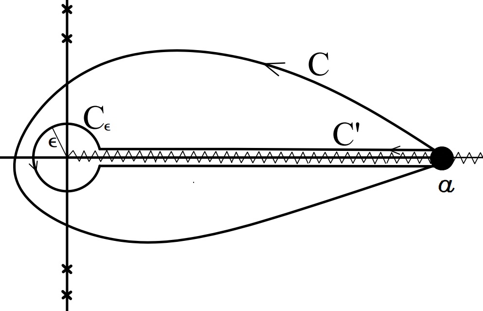
Figure 1. The contour $\mathrm{C}$ used in the representation (10) for the Hadamard’s finite part. The contour $\mathrm{C}$ excludes any of the poles of $f(z)$. The upper limit $a$ can be infinite. $\epsilon$ is a small positive parameter.

Hence, the finite part integral is

(21) $$\;\backslash\!\!\!\!\backslash\!\!\!\!\!\int_{0}^{\infty}\,\frac{e^{-bx}}{x^{m}}\,\mathrm{d}x=\lim^{\times}_{s\to 1-m}b^{-s}\Gamma(s)=\lim^{\times}_{s\to 1-m}\frac{\pi b^{-s}}{\sin(\pi s)\Gamma(1-s)}.$$

where we used the reflection formula $\Gamma(s)=\pi/\sin(\pi s)\Gamma(1-s)$. We then let $g(s)=\sin(\pi s)$ and $h(s)=\pi b^{-s}/\Gamma(1-s)$ so that from equation (15), the regularized limit evaluates to

(22) $$\;\backslash\!\!\!\!\backslash\!\!\!\!\!\int_{0}^{\infty}\,\frac{e^{-bx}}{x^{m}}\,\mathrm{d}x=\lim^{\times}_{s\to 1-m}\frac{h(s)}{g(s)}=\lim_{s\to 1-m}\frac{h^{\prime}(s)}{g^{\prime}(s)}.$$

Hence substituting $g^{\prime}(s)=\pi\cos(\pi s)$ and

(23) $$h^{\prime}(s)=-\frac{\pi b^{-s}}{\Gamma(1-s)}(\log b-\psi(1-s))$$

and computing the limit in equation (22) we obtain for the case when $b$ is real and positive,

(24) $$\;\backslash\!\!\!\!\backslash\!\!\!\!\!\int_{0}^{\infty}\,\frac{e^{-bx}}{x^{m}}\,\mathrm{d}x=\frac{\left(-1\right)^{m}\,b^{m-1}}{\left(m-1\right)!}\left(\ln\,b-\psi\left(m\right)\right),\qquad m=1,2\dots,$$

where $\psi\left(z\right)$ is the digamma function. This is consistent with the result in [37, eq 3.15] obtained after a lengthy calculation using the canonical definition (7). For the case when $b$ is imaginary, $b=-ia$ for any real $a$,

(25) $$\;\backslash\!\!\!\!\backslash\!\!\!\!\!\int_{0}^{\infty}\frac{e^{iax}}{x^{m}}\mathrm{d}x=-\frac{(ia)^{m-1}}{(m-1)!}\left(\ln|a|-\frac{i\pi}{2}\mathrm{sgn}(a)-\psi(m)\right),\qquad m=1,2\dots$$

In this particular case, the computation of the finite part integral (24) as a regularized limit is more convenient. In general however, especially for cases when the Mellin transform $\mathcal{M}[f(x);s]$ does not exist for some function $f(x)$, the Hadamard’s finite part integral can always be obtained from canonical definition (7).

3. Finite-Part Integration

An important application of the contour integral representation (10) is a technique known as finite-part integration [37, 42, 43, 44] and relies on the equivalence among the three different representations discussed above. The relevant procedure employed here is a special case of the more general result [45, eq 64]. We apply it here to give a rigorous derivation of the closed-form for the Heisenberg-Euler Lagrangian from which exact values can be computed. In the next section, we will use these values to check the results of a summation and extrapolation procedure applied on the divergent weak-field expansions of the Heisenberg-Euler Lagrangian.

3.1. The Heisenberg-Euler Lagrangian

The Heisenberg-Euler Lagrangian is a nonlinear correction to the Maxwell Lagrangian resulting from the interaction of a vacuum of charged particles of mass $m$ and spin $s$ with an external electromagnetic field [35, 46, 47, 48, 49, 50, 51]. In the one-loop order and for the case when the background field is constant and uniform, it depends on the invariant quantity $\beta=e^{2}(B^{2}-E^{2})/m^{4}$ where $e$ is the electron charge. For a purely electric background so that $\beta=-\kappa,\kappa=e^{2}E^{2}/m^{4}$, it is a complex-valued quantity and, for spin-$0$ particles, it admits the following integral representation in natural units $(h=c=1)$,

(26) $$\mathcal{L}_{0}{(\kappa)}=\frac{m^{4}}{16\pi^{2}}f_{0}(\kappa),\,\,\,f_{0}(\kappa)=-\int_{0}^{\infty}\frac{e^{-i\tau}}{\tau^{3}}\left[\sqrt{\kappa}\,\tau\,\mathrm{csch}\left(\sqrt{\kappa}\tau\right)-1+\frac{\kappa\tau^{2}}{6}\right]\mathrm{d}\tau.$$

In [36], we applied the method of finite-part integration on the corresponding representation in the case of a constant magnetic field background in which case the Heisenberg-Euler Lagrangian is real-valued. Similar to the magnetic case, the representation (26) is a finite sum of divergent integrals with pole singularities at the origin.

The initial step is to bring the integration into the complex plane with the use of the contour $\mathrm{C}$ in the representation (10) for the Hadamard’s finite part,

(27) $$\int_{\mathrm{C}}\frac{g(z)}{z^{3}}\log z\,\mathrm{d}z,\qquad g(z)=e^{-iz}\left[\sqrt{\kappa}\,z\,\mathrm{csch}\left(\sqrt{\kappa}z\right)-1+\frac{\kappa z^{2}}{6}\right],$$

where the contour $\mathrm{C}$ is given in figure 1 and $a$ can be taken to infinity. The poles due to $g(z)$ along the imaginary axis are exterior to $\mathrm{C}$ . We deform the contour $\mathrm{C}$ to an equivalent contour $\mathrm{C^{\prime}}$ so that

(28) $$\int_{\mathrm{C^{\prime}}}\frac{g(z)}{z^{3}}\log z\mathrm{d}z=2\pi i\int_{\epsilon}^{a}\frac{g(x)}{x^{3}}\mathrm{d}x+\int_{\mathrm{C}_{\epsilon}}\frac{g(z)}{z^{3}}\log z\,\mathrm{d}z,$$

where $\mathrm{C}_{\epsilon}$ is the circular contour about the origin. In the limit as $\epsilon\to 0$, the integral along the circular contour $\mathrm{C_{\epsilon}}$ vanishes so that equation (28) reduces to

(29) $$\int_{0}^{a}\frac{g(x)}{x^{3}}\mathrm{d}x=\frac{1}{2\pi i}\int_{\mathrm{C}}\frac{g(z)}{z^{3}}\log z\mathrm{d}z.$$

We then add a zero term,

(30) $$-\frac{\pi i}{2\pi i}\int_{\mathrm{C}}\frac{g(z)}{z^{3}}\mathrm{d}z=-\pi i\sum\mathrm{Res}\,\,\left[\frac{g(z)}{z^{3}}\right]=0,$$

to the right-hand side of equation (29) so that,

(31) $$\int_{0}^{a}\frac{g(x)}{x^{3}}\mathrm{d}x=\frac{1}{2\pi i}\int_{\mathrm{C}}\frac{g(z)}{z^{3}}\left(\log z-\pi i\right)\mathrm{d}z=\;\backslash\!\!\!\!\backslash\!\!\!\!\!\int_{0}^{a}\frac{g(x)}{x^{3}}\mathrm{d}x$$

where we used the contour integral representation (10) of the Hadamard’s finite part. Hence, taking the limit $a\to\infty$, the integral in the exact representation (26) evaluates to

(32) $$f_{0}(\kappa) =-\int_{0}^{\infty}\frac{e^{-i\tau}}{\tau^{3}}\left[\sqrt{\kappa}\,\tau\,\mathrm{csch}\left(\sqrt{\kappa}\tau\right)-1+\frac{\kappa\tau^{2}}{6}\right]\mathrm{d}\tau$$

(33) $$=-\sqrt{\kappa}\,\;\backslash\!\!\!\!\backslash\!\!\!\!\!\int_{0}^{\infty}\frac{e^{-i\tau}\mathrm{csch}(\sqrt{\kappa}\tau)}{\tau^{2}}\mathrm{d}\tau+\;\backslash\!\!\!\!\backslash\!\!\!\!\!\int_{0}^{\infty}\frac{e^{-i\tau}}{\tau^{3}}\mathrm{d}\tau-\frac{\kappa}{6}\;\backslash\!\!\!\!\backslash\!\!\!\!\!\int_{0}^{\infty}\frac{e^{-i\tau}}{\tau}\mathrm{d}\tau.$$

In effect, the result (33) follows directly from a term-by-term integration followed by the immediate regularization of the divergent terms as Hadamard’s finite part. In section 4, we will demonstrate that this procedure will generally result to missing terms especially when one performs a term-by-term integration involving an infinite number of divergent integrals.

The finite part integrals in right-hand side of equation (33) can be computed from the following Mellin transform integral [41, p 34],

$$\mathcal{M}\left[e^{-a\tau}\mathrm{csch}{\left(b\,\tau\right)};\,\,s\right] =\int_{0}^{\infty}\tau^{s-1}e^{-a\tau}\mathrm{csch}{\left(b\,\tau\right)}\mathrm{d}\tau$$

(34) $$=\frac{2^{1-s}}{b^{s}}\Gamma(s)\,\zeta\left(s,\frac{a+b}{2\,b}\right),\qquad\mathrm{Re}\,a>-|\mathrm{Re}\,b|;\mathrm{Re}\,s>1,$$

where $\,\zeta\left(z,\nu\right)$ is the Hurwitz zeta function. The finite part integral is the regularized limit at the pole $s=-1$ of the analytic continuation of the Mellin transform to the whole complex plane which is given simply by the right-hand side of equation (34),

(35) $$\mathcal{M}^{\ast}\left[e^{-a\tau}\mathrm{csch}{\left(b\,\tau\right)};\,\,s\right]=\frac{2^{1-s}}{b^{s}}\Gamma(s)\,\zeta\left(s,\frac{a+b}{2\,b}\right).$$

So that

(36) $$\;\backslash\!\!\!\!\backslash\!\!\!\!\!\int_{0}^{\infty}\frac{e^{-i\tau}\,\mathrm{csch}(\sqrt{\kappa}\tau)}{\tau^{2}}\mathrm{d}\tau =\lim_{s\to-1}^{\times}\mathcal{M}^{\ast}\left[e^{-i\tau}\mathrm{csch}{\left(\sqrt{\kappa}\tau\right)};s\right]$$

(37) $$=\lim_{s\to-1}^{\times}\frac{2\pi(2\sqrt{\kappa})^{-s}}{\sin(\pi s)\Gamma(1-s)}\zeta\!\left(s,\frac{\sqrt{\kappa}+i}{2\sqrt{\kappa}}\right),$$

where we made use of the reflection formula for $\Gamma(s)=\pi/\sin(\pi s)\Gamma(1-s)$. We then rationalize the analytic continuation (37) as,

(38) $$\mathcal{M}^{\ast}\left[e^{-i\tau}\mathrm{csch}{\left(\sqrt{\kappa}\,\tau\right)};\,\,s\right]=\frac{h(s)}{g(s)},$$

where

(39) $$h(s)=\frac{2\pi(2\sqrt{\kappa})^{-s}}{\Gamma(1-s)}\zeta\left(s,\frac{\sqrt{\kappa}+i}{2\sqrt{\kappa}}\right),\qquad g(s)=\sin(\pi s).$$

Hence, from the formula (15), the regularized limit is given by

(40) $$\;\backslash\!\!\!\!\backslash\!\!\!\!\!\int_{0}^{\infty}\frac{e^{-i\tau}\,\mathrm{csch}(\sqrt{\kappa}\tau)}{\tau^{2}}\mathrm{d}\tau=\lim_{s\to-1}^{\times}\frac{h(s)}{g(s)}=\lim_{s\to-1}\frac{h^{\prime}(s)}{g^{\prime}(s)}.$$

where $g^{\prime}(s)=\pi\cos(\pi s)$ and

$$h^{\prime}(s)=\frac{2(2\sqrt{\kappa})^{-s}\pi}{\Gamma(1-s)} \left[\left(\psi(1-s)-\ln\left(2\sqrt{\kappa}\right)\right)\,\zeta\left(s,\frac{\sqrt{\kappa}+i}{2\sqrt{\kappa}}\right)\right.$$

(41) $$+ \left.\,\zeta^{(1,0)}\left(s,\frac{\sqrt{\kappa}+i}{2\sqrt{\kappa}}\right)\right],$$

so that,

$$\;\backslash\!\!\!\!\backslash\!\!\!\!\!\int_{0}^{\infty}\frac{e^{-i\tau}\,\mathrm{csch}(\sqrt{\kappa}\tau)}{\tau^{2}}\mathrm{d}\tau=-4\sqrt{\kappa} \left[\left(\psi(2)-\ln\left(2\sqrt{\kappa}\right)\right)\,\zeta\left(-1,\frac{\sqrt{\kappa}+i}{2\sqrt{\kappa}}\right)\right.$$

(42) $$+ \left.\,\zeta^{(1,0)}\left(-1,\frac{\sqrt{\kappa}+i}{2\sqrt{\kappa}}\right)\right].$$

The other finite part integrals in the right-hand side of equation (33) are special cases of the result (25). Substituting the finite-part integral (42) to equation (33), we obtain

$$f_{0}(\kappa)=\frac{\kappa}{6}-\frac{1}{4}-\left(\frac{\kappa}{6}+\frac{1}{2}\right)\ln{\left(2\sqrt{\kappa}\right)}+ i\left(\frac{\pi}{4}+\frac{\kappa\pi}{12}\right)$$

(43) $$+4\kappa\,\zeta^{(1,0)}\left(-1,\frac{\sqrt{\kappa}+i}{2\sqrt{\kappa}}\right)$$

where we’ve made use of the formula [61]

(44) $$\zeta(-1,\nu)=-\frac{1}{12}+\frac{\nu}{2}-\frac{\nu^{2}}{2}.$$

The real and imaginary parts are then given by

(45) $$\mathrm{Re}\,f_{0}(\kappa)=\frac{\kappa}{6}-\frac{1}{4}-\left(\frac{\kappa}{6}+\frac{1}{2}\right)\ln{\left(2\sqrt{\kappa}\right)}+4\kappa\,\mathrm{Re}\left[\zeta^{(1,0)}\left(-1,\frac{\sqrt{\kappa}+i}{2\sqrt{\kappa}}\right)\right]$$

and

(46) $$\mathrm{Im}\,f_{0}(\kappa)=\frac{\pi}{4}+\frac{\kappa\pi}{12}+4\kappa\,\mathrm{Im}\left[\zeta^{(1,0)}\left(-1,\frac{\sqrt{\kappa}+i}{2\sqrt{\kappa}}\right)\right].$$

As suggested in [47], a result numerically consistent with (43) can be obtained by a suitable analytic continuation, $B\to-iE$, of the corresponding closed-form [36, eq 42] for the case of a magnetic background. This procedure must be carefully implemented by choosing an appropriate branch for the complex logarithmic function and the Hurwitz zeta functions appearing in [36, eq 42]. In particular, we find that the branch $\log(iy)=\ln y+i\pi/2$ is compatible with Mathematica 13.2 ’s implementation for $\zeta\left(-1,x+iy\right)$ and $\zeta^{(1,0)}\left(-1,x+iy\right)$ for any $x,y>0$, to give a numerical value consistent with that computed from (43).

3.2. Spin-$\frac{1}{2}$

Similarly in the case of spinor QED, the Heisenberg-Euler Lagrangian for a purely electric background is given by the exact integral representation

(47) $$\mathcal{L}_{\frac{1}{2}}{(\kappa)}=\frac{m^{4}}{8\pi^{2}}f_{\frac{1}{2}}(\kappa),\,\,\,f_{\frac{1}{2}}(\kappa)=\int_{0}^{\infty}\frac{e^{-i\,\tau}}{\tau^{3}}\left[\sqrt{\kappa}\,\tau\coth\left(\sqrt{\kappa}\,\tau\right)-1-\frac{\kappa\,\tau^{2}}{3}\right]\mathrm{d}\tau.$$

Employing finite-part integration as in the previous case,

(48) $$f_{\frac{1}{2}}(\kappa)=\sqrt{\kappa}\;\backslash\!\!\!\!\backslash\!\!\!\!\!\int_{0}^{\infty}\frac{e^{-i\,\tau}\,\coth\left(\sqrt{\kappa}\,\tau\,\right)}{\tau^{2}}\mathrm{d}\tau-\;\backslash\!\!\!\!\backslash\!\!\!\!\!\int_{0}^{\infty}\frac{e^{-i\,\tau}}{\tau^{3}}\mathrm{d}\tau-\frac{\kappa}{3}\;\backslash\!\!\!\!\backslash\!\!\!\!\!\int_{0}^{\infty}\frac{e^{-i\,\tau}}{\tau}\mathrm{d}\tau.$$

The first finite part integral on the right-hand side of equation (48) is the regularized limit of the analytic continuation to the whole complex plane of the Mellin transform integral [41, p. 34]. The procedure is similar to that performed in equation (42) and the result is given by

$$\;\backslash\!\!\!\!\backslash\!\!\!\!\!\int_{0}^{\infty}\frac{e^{-i\,\tau}\,\coth\left(\sqrt{\kappa}\,\tau\right)}{\tau^{2}}\mathrm{d}\tau=i(1-\gamma) +\frac{\pi}{2}+2\sqrt{\kappa}\left(2(\gamma-1)+\ln(4\kappa)\right)\zeta\left(-1,\frac{i}{2\sqrt{\kappa}}\right)$$

(49) $$-4\sqrt{\kappa}\,\zeta^{(1,0)}\left(-1,\frac{i}{2\sqrt{\kappa}}\right),$$

where $\gamma=-\psi(1)$ is the Euler-Mascheroni constant. The other finite part integrals in the right-hand side of equation (48) are again special cases of equation (25) so that

$$f_{\frac{1}{2}}(\kappa)=\frac{1}{4}+\frac{\pi\sqrt{\kappa}}{2} +\frac{\kappa}{3}-\frac{\kappa\ln{(4\kappa)}}{6}+\frac{\ln{(4\kappa)}}{4}-4\kappa\,\zeta^{(1,0)}\left(-1,\frac{i}{2\sqrt{\kappa}}\right)$$

(50) $$+i\left(-\frac{\pi}{4}+\frac{\kappa\pi}{6}+\frac{\sqrt{\kappa}\ln{(4\kappa)}}{2}\right).$$

where we again made use of the property (44). The result (50) is also numerically equal to that obtained by an appropriate analytic continuation, $B\to-iE$, of the corresponding closed-form [46, eq 1.47] for the Heisenberg-Euler Lagrangian in the magnetic case. We again chose $\log(iy)=\ln y+i\pi/2$ for any real $y>0$.

3.3. Self-dual electromagnetic background.

In the case when the electromagnetic background is self-dual (SD) [46, 53, 54, 55, 56] satisfying

(51) $$F_{\mu\nu}=\widetilde{F}_{\mu\nu}\equiv\frac{1}{2}\epsilon_{\mu\nu\rho\lambda}F^{\rho\lambda},$$

the Heisenberg-Euler Lagrangian describing a charged scalar particle is given by

(52) $$\mathcal{L}_{\mathrm{SD}}(\beta)=\frac{e^{2}\mathcal{F}^{2}}{4\pi^{2}}f_{\mathrm{SD}}(\beta),\,\,\,f_{\mathrm{SD}}(\beta)=\frac{1}{4}\int_{0}^{\infty}\frac{\mathrm{d}\tau}{\tau}\left(\frac{1}{\sinh^{2}{\tau}}-\frac{1}{\tau^{2}}+\frac{1}{3}\right)e^{-{2\tau}/{\sqrt{\beta}}}$$

where $\mathcal{F}^{2}=\frac{1}{4}F_{\mu\nu}F^{\mu\nu}$ and the natural dimensionless parameter $\sqrt{\beta}=2e\mathcal{F}/m^{2}$. The integral, $f_{\mathrm{SD}}(\beta)$, also appears in the effective Lagrangian in the case of spinor QED. It is also relevant in the study of nonperturbative phenomena in topological string theory and in the $c=1$ string theory at self-dual radius [53]. A weak-field expansion for $f_{\mathrm{SD}}(\beta)$ is given by [56],

(53) $$f_{\mathrm{SD}}(\beta)\sim\beta\sum_{n=0}^{\infty}-\frac{(-1)^{n}B_{2n+4}}{(2n+2)(2n+4)}(-\beta)^{n},\qquad\beta\to 0.$$

For a real or magnetic-like background $\mathcal{F}$, $\mathcal{L}_{0}(\beta)$ is real and PT expansion (53) is alternating. For the case when the background is imaginary, $\mathcal{F}=-i\overline{\mathcal{F}}$ or electric-like, the Heisenberg-Euler Lagrangian is complex-valued and is given by,

(54) $$\mathcal{L}_{\text{SD}}(\kappa) =\frac{e^{2}\overline{\mathcal{F}}^{2}}{4\pi^{2}}f_{\text{SD}}(\kappa),\,\,\,f_{\text{SD}}(\kappa)=-\frac{1}{4}\int_{0}^{\infty}\frac{\mathrm{d}\tau}{\tau}\left(\frac{1}{\sinh^{2}{\tau}}-\frac{1}{\tau^{2}}+\frac{1}{3}\right)e^{-{2i\tau}/{\sqrt{\kappa}}}.$$

where $\sqrt{\kappa}=2e\overline{\mathcal{F}}/m^{2}$. As in the previous cases, a closed-form for the integral $f_{\text{SD}}(\kappa)$ can be derived by finite-part integration,

(55) $$f_{\text{SD}}(\kappa)=-\frac{1}{4}\;\backslash\!\!\!\!\backslash\!\!\!\!\!\int_{0}^{\infty}\frac{e^{-{2i\tau}/{\sqrt{\kappa}}}}{\tau\sinh^{2}{\tau}}\mathrm{d}\tau+\frac{1}{4}\;\backslash\!\!\!\!\backslash\!\!\!\!\!\int_{0}^{\infty}\frac{e^{-{2i\tau}/{\sqrt{\kappa}}}}{{\tau^{3}}}\mathrm{d}\tau-\frac{1}{12}\;\backslash\!\!\!\!\backslash\!\!\!\!\!\int_{0}^{\infty}\frac{e^{-{2i\tau}/{\sqrt{\kappa}}}}{{\tau}}\mathrm{d}\tau.$$

The finite part integral in the first term is computed as a regularized limit of the analytic continuation of the Mellin transform integral [41, p 29, eq 10] so that

$$\frac{1}{4}\;\backslash\!\!\!\!\backslash\!\!\!\!\!\int_{0}^{\infty}\frac{e^{-{2i\tau}/{\sqrt{\kappa}}}}{\tau\sinh^{2}{\tau}}\mathrm{d}\tau= \left(\psi(1)-\ln 2\right)\left(\zeta\left(-1,\frac{i}{\sqrt{\kappa}}\right)-\frac{i}{\sqrt{\kappa}}\zeta\left(0,\frac{i}{\sqrt{\kappa}}\right)\right)$$

(56) $$+\zeta^{(1,0)}\left(-1,\frac{i}{\sqrt{\kappa}}\right)-\frac{i}{\sqrt{\kappa}}\zeta^{(1,0)}\left(0,\frac{i}{\sqrt{\kappa}}\right).$$

The other finite part integrals in the right-hand side of equation (55) are again special cases of the finite part integral given in equation (25). We then use the following results for the Hurwitz zeta function

(57) $$\zeta\left(0,\frac{i}{\sqrt{\kappa}}\right)=\frac{1}{2}-\frac{i}{\sqrt{\kappa}},\qquad\zeta\left(-1,\frac{i}{\sqrt{\kappa}}\right)=\frac{1}{2\kappa}+\frac{i}{2\sqrt{\kappa}}-\frac{1}{12}$$

to simplify the result and obtain,

(58) $$f_{\text{SD}}(\kappa)=\frac{i}{\sqrt{\kappa}}\zeta^{(1,0)}\left(0,\frac{i}{\sqrt{\kappa}}\right) -\zeta^{(1,0)}\left(-1,\frac{i}{\sqrt{\kappa}}\right)$$

$$-\frac{1}{4\kappa}\left(\ln\kappa+3\right)-\frac{\ln\kappa}{24}+\pi i\left(\frac{1}{24}+\frac{1}{4\kappa}\right).$$

As in the previous cases, the result (58) gives consistent numerical values by performing a suitable analytic continuation, $\mathcal{F}\to-i\overline{\mathcal{F}}$, on the corresponding closed-form for a real magnetic-like background in [36] which we also derived using finite-part integration.

4. Summation and extrapolation of the weak-field expansion for the Heisenberg-Euler Lagrangian

We now discuss the main result of this paper which is the application of the method of finite-part integration on the resummation of divergent nonalternating PT expansion. In particular, we will piece together a convergent extrapolant that enables us to compute the complex-valued Heisenberg-Euler Lagrangian in the strong electric field limit from the real coefficients of the divergent weak-field expansion.

In the case of the scalar QED, a formal representation is obtained from the exact representation (26) by a rotation, $i\tau=t$, so that formally [46],

(59) $$f_{0}(\kappa)=\int_{0}^{\infty}\frac{e^{-t}}{t^{3}}\left(\sqrt{\kappa}\,t\csc\left(\sqrt{\kappa}t\right)-1-\frac{\kappa t}{6}\right)\mathrm{d}t,\qquad\kappa=\frac{e^{2}E^{2}}{m^{4}}.$$

Then a divergent weak-field PT expansion is obtained by replacing the factor in the parenthesis by an expansion about $\kappa=0$ and carrying out a term-by-term integration that yields,

(60) $$f_{0}(\kappa)\sim\kappa^{2}\sum_{n=0}^{\infty}\frac{(-1)^{n}\overline{\mathcal{B}}_{2n+4}2^{2n+4}}{(2n+4)(2n+3)(2n+2)}\kappa^{n},\qquad\kappa\to 0^{+},$$

where the constants $\overline{\mathcal{B}}_{2n}$ are in terms of the Bernoulli numbers, $B_{2n}$,

(61) $$\overline{\mathcal{B}}_{2n}=\frac{\left(1-2^{2n-1}\right)}{2^{2n-1}}B_{2n}.$$

The imaginary part comes from the contributions of the poles along the integration path in the real line in the formal representation (59). A convergent weak-field expansion can be obtained from (59) using the method of residues. The result is given by [46, 51],

(62) $$\mathrm{Im}f_{0}(\kappa)=\frac{\kappa}{\pi}\sum_{n=1}^{\infty}\frac{(-1)^{n+1}}{n^{2}}\exp\left(-\frac{n\pi}{\sqrt{\kappa}}\right).$$

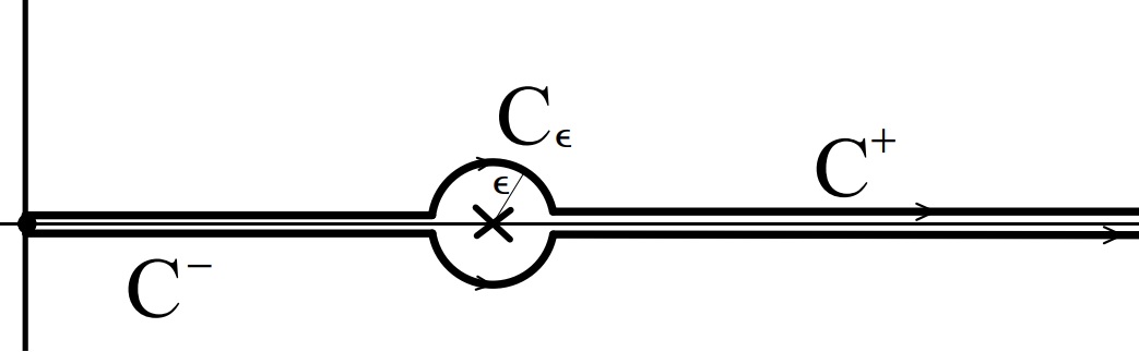
Figure 2. The contours of integration, $\mathrm{C}^{+}$ and $\mathrm{C}^{-}$ used in the prescription for evaluating the integral in (71). They correspond to two directions with which the half-circle about the pole $\mathrm{C}_{\epsilon}$ is traversed.

Similarly for the case of spinor QED, the Heisenberg-Euler Lagrangian (47) assumes the following formal representation after the rotation $i\tau=t$,

(63) $$f_{\frac{1}{2}}(\kappa)=-\int_{0}^{\infty}\frac{e^{-t}}{t^{3}}\left(\sqrt{\kappa}\,t\cot\left(\sqrt{\kappa}\,t\right)-1+\frac{\kappa\,t^{2}}{3}\right)\mathrm{d}t,$$

from which a divergent weak-field expansion for the real part is obtained,

(64) $$f_{\frac{1}{2}}(\kappa)\sim\kappa^{2}\sum_{n=0}^{\infty}\frac{(-1)^{n+1}B_{2n+4}2^{2n+4}}{(2n+4)(2n+3)(2n+2)}\kappa^{n}.$$

Furthermore, a convergent expansion for the imaginary part, $\mathrm{Im}f_{\frac{1}{2}}(\kappa)$, can be derived similarly from the formal representation (63) using the method of residue [46],

(65) $$\mathrm{Im}f_{\frac{1}{2}}(\kappa)=\frac{\kappa}{\pi}\sum_{n=1}^{\infty}\frac{1}{n^{2}}\exp\left(-\frac{n\pi}{\sqrt{\kappa}}\right).$$

In both spin cases, the coefficients of the weak-field expansions (60) and (64) possess a leading $a_{2n}^{(s)}\sim(2n)!$ growth as $n\to\infty$. We present in table 1, the partial sums of the expansion (60) to compute $\mathrm{Re}f_{0}(\kappa)$ for some values of the parameter $\kappa$. The exponentially vanishing imaginary parts (62) and (65) of the Heisenberg-Euler Lagrangian in both cases are invisible up to any finite order of the corresponding weak-field perturbation expansions

Furthermore, in the purely magnetic case, $\beta=(eB)^{2}/m^{4}$, the Heisenberg-Euler Lagrangians possess the following leading behavior in the strong-magnetic field regime [46, eqs 1.63 and 1.54],

(66) $$f_{0}(\beta)\sim\frac{\beta\ln\beta}{12}+\frac{\ln 2}{6}\beta+\dots\,\,\,\text{and}\,\,\,f_{\frac{1}{2}}(\beta)\sim\frac{\beta\ln\beta}{6}+\frac{\ln 2}{3}\beta+\dots$$

By analytic continuation, $B\to-iE$, the real and imaginary parts of the Heisenberg-Euler Lagrangians in a purely electric field background will exhibit the following leading-order behaviors in the strong electric field regime [47],

(67) $$\mathrm{Re}f_{s}(\kappa)\sim\kappa\ln\kappa+\kappa,\qquad\mathrm{Im}f_{s}(\kappa)\sim\kappa,\qquad\kappa\to\infty.$$

$d$	$\kappa=0.01$	$\kappa=0.1$	$\kappa=0.2$
1	${\color[rgb]{0,0,1}1.95}67460317460(10^{-6})$	${\color[rgb]{0,0,1}2}.06746032(10^{-4})$	8.7619$(10^{-4})$
3	${\color[rgb]{0,0,1}1.95700}87692400(10^{-8})$	${\color[rgb]{0,0,1}2.10}341210(10^{-4})$	9.509187109$(10^{-4})$
5	${\color[rgb]{0,0,1}1.9570096}417862(10^{-6})$	${\color[rgb]{0,0,1}2.1}2001352(10^{-4})$	1.1131746$(10^{-3})$
9	${\color[rgb]{0,0,1}1.957009659}6544(10^{-6})$	${\color[rgb]{0,0,1}2}.52547209(10^{-4})$	6.88452$(10^{-2})$
20	${\color[rgb]{0,0,1}1.9570096}601688(10^{-6})$	$9.50638258(10^{5})$
50	$4.1365574383679(10^{4})$
Exact	$1.9570096599269(10^{-6})$	$2.10778565(10^{-4})$	$9.19523360907(10^{-4})$

Table 1. Convergence of the perturbative expansion (60) for the real part of $f_{0}(\kappa)$ in the Heisenberg-Euler Lagrangian in the case of a scalar QED. The exact result is computed from the closed-form (45).

On the basis of this information, we map the nonalternating coefficients, $a_{n}^{(s)}$, in the divergent expansions (60) and (64) to the positive-power moments, $\mu_{2n}^{(s)}$, of some positive function $\rho_{s}(x)$,

(68) $$a_{n}^{(s)}=\mu_{2n}^{(s)}=\int_{0}^{\infty}x^{2n}\rho_{s}(x)\mathrm{d}x,\qquad n=0,1,\dots$$

This particular mapping is motivated by the leading $(2n)!$ growth of the expansion coefficients, $a_{n}^{(s)}$, and in anticipation of the leading exponential behavior of the reconstruction for $\rho_{s}(x)$ from the moments $\mu_{2n}$ which we will carry out later in the section.

Hence, the divergent expansions for $f_{s}(\kappa)$ can be summed formally as

$$f_{s}(\kappa) =\kappa^{2}\sum_{n=0}^{\infty}\int_{0}^{\infty}x^{2n}\rho_{s}(x)(\kappa)^{n}\mathrm{d}x=\kappa^{2}\int_{0}^{\infty}\rho_{s}(x)\left(\sum_{n=0}^{\infty}(\kappa x^{2})^{n}\right)\mathrm{d}x$$

(69) $$=\kappa^{2}\,\int_{0}^{\infty}\frac{\rho_{s}(x)}{1-\kappa x^{2}}\mathrm{d}x=\kappa H(\kappa).$$

which is in terms of the formal integral

(70) $$H_{s}(\kappa)=\int_{0}^{\infty}\frac{\rho_{s}(x)}{1/\kappa-x^{2}}\mathrm{d}x.$$

The integration can be carried out by a suitable prescription for the deformation of the contour. Two such prescriptions are shown in figure 2. In the limit as $\epsilon\to 0$, we obtain

(71) $$H_{s}(\kappa)=\mathrm{PV}\int_{0}^{\infty}\frac{\,\rho_{s}(x)}{1/\kappa-x^{2}}\mathrm{d}x\pm i\frac{\pi\sqrt{\kappa}}{2}\rho_{s}\left(\frac{1}{\sqrt{\kappa}}\right).$$

where the plus(minus) sign corresponds to performing the integration along the path $\mathrm{C}^{+(-)}$. Yet another possibility is to deform the contour in a manner that renders the imaginary part in (71) extraneous so that $H(\kappa)$ is real-valued and is given by the Cauchy principal value integral. In general, the manner in which this is done is unclear from perturbation theory alone and a separate prescription must be provided to clear this nonperturbative ambiguity. In the case of the Heisenberg-Euler Lagrangian, the imaginary part gives the particle-antiparticle pair production rate, $\Gamma_{\text{prod}}(\kappa)=2\mathrm{Im}\left(f_{s}(\kappa)\right)$, so that the appropriate contour is $\mathrm{C^{+}}$.

Finally, the Cauchy principal value in the right-hand side of equation (71) can be computed explicitly using finite-part integration. This allows us to incorporate the strong field constraint (67). This is given in the following theorem. An independent but equivalent derivation is also given in [52].

Theorem 4.1.

Let the complex extension, $\rho(z)$, of the real-valued function $\rho(x)$ along the real line, be entire, then

(72) $$\mathrm{PV}\int_{0}^{\infty}\frac{\rho(x)}{1/\kappa-x^{2}}\mathrm{d}x=-\sum_{n=0}^{\infty}\frac{\mu_{-(2n+2)}}{\kappa^{n}}-\Delta(\kappa),$$

where the term $\Delta(\kappa)$ is given by

(73) $$\Delta(\kappa)=\frac{\sqrt{\kappa}}{2}\ln\left(\sqrt{\kappa}\right)\left(\rho\left(\frac{1}{\sqrt{\kappa}}\right)-\rho\left(-\frac{1}{\sqrt{\kappa}}\right)\right).$$

and $\mu_{-(2k+2)}$, the divergent negative-power moments of $\rho(x)$, are Hadamard’s finite part integrals,

(74) $$\mu_{-(2n+2)}=\;\backslash\!\!\!\!\backslash\!\!\!\!\!\int_{0}^{\infty}\frac{\rho(x)}{x^{2n+2}}\mathrm{d}x.$$

Proof.

Deform the contour $\mathrm{C}$ to $\mathrm{C^{\prime}}$ as shown in figure 3 and perform the following contour integration,

$$\int_{\mathrm{C^{\prime}}}\frac{\rho(z)}{1/\kappa-z^{2}}\,\log z\mathrm{d}z=2\pi i\,\mathrm{PV} \int_{0}^{a}\frac{\rho(x)}{1/\kappa-x^{2}}\mathrm{d}x+\int_{\mathrm{C}_{\epsilon_{1}}}\frac{\rho(z)}{1/\kappa-z^{2}}\log z\mathrm{d}z$$

(75) $$+\int_{\mathrm{C}_{\epsilon_{2}}}\frac{\rho(z)}{1/\kappa-z^{2}}\log z\mathrm{d}z,$$

where the contour integral around the circular loop $\mathrm{C_{\epsilon}}$ vanishes as $\epsilon\to 0$ and the first term of the right-hand side of equation (75) containing the desired principal value integral is the sum of the integrals along the segments labelled $1,2,5$ and $6$ in the limit as $\epsilon,\epsilon_{2}\to 0$. The remaining integrals in the right-hand side of equation (75) are evaluated as

$$\lim_{\epsilon_{2}\to 0}\int_{\mathrm{C}_{\epsilon_{2}}}\frac{\rho(z)}{1/\kappa-z^{2}}\log z\mathrm{d}z=-(2\pi i) \left[\frac{\sqrt{\kappa}}{2}\rho\left(\frac{1}{\sqrt{\kappa}}\right)\ln\left(\frac{1}{\sqrt{\kappa}}\right)\right.$$

(76) $$+\left.\pi i\mathrm{Res}\left[\frac{\rho(z)}{z^{2}-1/\kappa};z=\frac{1}{\sqrt{\kappa}}\right]\right].$$

and

$$\lim_{\epsilon_{1}\to 0}\int_{\mathrm{C}_{\epsilon_{1}}}\frac{\rho(z)}{1/\kappa-z^{2}}\log z\mathrm{d}z=(2\pi i) \left[\frac{\sqrt{\kappa}}{2}\rho\left(-\frac{1}{\sqrt{\kappa}}\right)\ln\left(\frac{1}{\sqrt{\kappa}}\right)\right.$$

(77) $$-\left.\pi i\mathrm{Res}\left[\frac{\rho(z)}{z^{2}-1/\kappa};z=-\frac{1}{\sqrt{\kappa}}\right]\right].$$

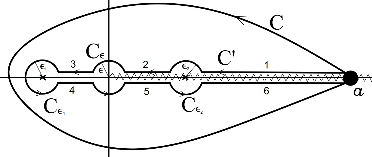
Figure 3. The contour of integration used for the evaluation of the principal value integral (72). Poles located at $z=\pm 1/\sqrt{\kappa}$ are in the interior of the contour $\mathrm{C}$.

Substituting these to equation (75) and solving for the principal value integral we obtain,

$$\mathrm{PV}\int_{0}^{a}\frac{\rho(x)}{1/\kappa-x^{2}}\mathrm{d}x=\frac{1}{2\pi i} \int_{\mathrm{C}}\frac{\rho(z)(\log z-\pi i)}{1/\kappa-z^{2}}\mathrm{d}z$$

(78) $$+\frac{\sqrt{\kappa}}{2}\ln\left(\frac{1}{\sqrt{\kappa}}\right)\left(\rho\left(\frac{1}{\sqrt{\kappa}}\right)-\rho\left(-\frac{1}{\sqrt{\kappa}}\right)\right),$$

where we made use of

(79) $$\pi i\sum\mathrm{Res}\left[\frac{\rho(z)}{z^{2}-1/\kappa};z=\pm\frac{1}{\sqrt{\kappa}}\right]=-\frac{\pi i}{2\pi i}\int_{\mathrm{C}}\frac{\rho(z)}{1/\kappa-z^{2}}\mathrm{d}z.$$

In the first term in the right-hand side of equation (78), we expand $(1/\kappa-z^{2})^{-1}$ in powers of $1/(\kappa z^{2})$ and implement a term-by-term integration,

(80) $$\frac{1}{2\pi i}\int_{\mathrm{C}}\frac{\rho(z)(\log z-\pi i)}{1/\kappa-z^{2}}\mathrm{d}z= -\sum_{n=0}^{\infty}\frac{1}{\kappa^{n}}\frac{1}{2\pi i}\int_{\mathrm{C}}\frac{\rho(z)(\log z-\pi i)}{z^{2n+2}}\mathrm{d}z$$

(81) $$= -\sum_{n=0}^{\infty}\frac{1}{\kappa^{n}}\;\backslash\!\!\!\!\backslash\!\!\!\!\!\int_{0}^{a}\frac{\rho(x)}{x^{2n+2}}\mathrm{d}x,\,\,|z|>\frac{1}{\sqrt{\kappa}}$$

where in equation (81), we used the contour integral representation (10) of the Hadamard’s finite part integral. Substituting equation (81) for the first term of the right-hand side of equation (78) and taking the limit as $a\to\infty$,

$$\lim_{a\to\infty}\mathrm{PV}\int_{0}^{a}\frac{\rho(x)}{1/\kappa-x^{2}}\mathrm{d}x= -\sum_{n=0}^{\infty}\frac{1}{\kappa^{n}}\lim_{a\to\infty}\;\backslash\!\!\!\!\backslash\!\!\!\!\!\int_{0}^{a}\frac{\rho(x)}{x^{2n+2}}\mathrm{d}x$$

(82) $$+\frac{\sqrt{\kappa}}{2}\ln\left(\frac{1}{\sqrt{\kappa}}\right)\left(\rho\left(\frac{1}{\sqrt{\kappa}}\right)-\rho\left(-\frac{1}{\sqrt{\kappa}}\right)\right),$$

This proves the result (72). ∎

In the purely magnetic case, $\kappa\to-\beta,\beta=e^{2}B^{2}/m^{4}$, so that the weak field expansions (60) and (64) are alternating, the prescription (68) sums the divergent expansions to a generalized Stieltjes integral, $f_{s}(\beta)=\beta S_{s}(\beta)$, which we also evaluated exactly in [36] using finite-part integration to give

(83) $$S_{s}(\beta)=\int_{0}^{\infty}\frac{\rho_{s}(x)}{1/\beta+x^{2}}\mathrm{d}x=\sum_{n=0}^{\infty}\frac{(-1)^{n}}{\beta^{n}}\mu_{-(2n+2)}^{(s)}+\Lambda(\beta),$$

where the term $\Lambda(\beta)$ is given by

(84) $$\Lambda(\beta)=\frac{\pi\sqrt{\beta}}{4}\left(\rho\left(\frac{i}{\sqrt{\beta}}\right)+\rho\left(\frac{-i}{\sqrt{\beta}}\right)\right)+\frac{\sqrt{\beta}\ln\beta}{4i}\left(\rho\left(\frac{i}{\sqrt{\beta}}\right)-\rho\left(\frac{-i}{\sqrt{\beta}}\right)\right).$$

The regularization carried out in equation (71) for the formal integral $H_{s}(\kappa)$ can then be recovered naturally by performing an analytic continuation, $S_{s}(\beta\to-\kappa)$, on equation (83) to the branch cut of $S_{s}(\beta)$ along the negative real line in the complex-$\beta$ plane. The sign in the second term of the right hand side of (71) now corresponds to whether the branch cut is approached from above ($+$) or below ($-$). In the case of the Heisenberg-Euler Lagrangian, the approach should come from above to yield a positive imaginary part.

The expansion in the first term of the right-hand side of (72) can be shown to be absolutely convergent (see the proof of Theorem 3.1 in [52]). This convergence and the existence of the limit (8) justify interchanging the limit operation with the infinite sum in equation (82). Meanwhile, the term $\Delta(\kappa)$ is missed by merely performing a formal term-by-term integration followed by an immediate regularization of the divergent integrals by Hadamard’s finite part. This term provides the dominant behavior of the principal value integral (72) as $\kappa\to\infty$. It originates from contributions of the poles $z=\pm 1/\sqrt{\kappa}$ interior to the contour $\mathrm{C}$ in figure 3 which results from the uniformity condition imposed in equation (81).

By contrast, the finite-part integration (33) of the integral representation for the Heisenberg-Euler Lagrangian involves term-by-term integration over a finite number of divergent integrals so that no uniformity condition is imposed and consequently, the contour $\mathrm{C}$ in figure 1 excludes any of the poles of the integrand along the imaginary axis.

Moments	$\kappa=1$	$\kappa=4$
200	${\color[rgb]{0,0,1}0.0209}01957+i{\color[rgb]{0,0,1}0.0136}6231$	${\color[rgb]{0,0,1}0.102}1807+i{\color[rgb]{0,0,1}0.25}054011$
500	${\color[rgb]{0,0,1}0.02094}3108+i{\color[rgb]{0,0,1}0.0136}10668$	${\color[rgb]{0,0,1}0.1022}391+i{\color[rgb]{0,0,1}0.2520}3733$
800	${\color[rgb]{0,0,1}0.020942}796+i{\color[rgb]{0,0,1}0.0136}10094$	${\color[rgb]{0,0,1}0.1022}458+i{\color[rgb]{0,0,1}0.2520}5037$
1000	${\color[rgb]{0,0,1}0.02094}3004+i{\color[rgb]{0,0,1}0.013609}780$	${\color[rgb]{0,0,1}0.1022}316+i{\color[rgb]{0,0,1}0.2520}5760$
1500	${\color[rgb]{0,0,1}0.02094296}2+i{\color[rgb]{0,0,1}0.013609}607$	${\color[rgb]{0,0,1}0.10222}66+i{\color[rgb]{0,0,1}0.25206}534$
2000	${\color[rgb]{0,0,1}0.02094296}8+i{\color[rgb]{0,0,1}0.013609}603$	${\color[rgb]{0,0,1}0.10222}63+i{\color[rgb]{0,0,1}0.252064}87$
$P^{999}_{1000}(\kappa)$	$0.040044268$	$-0.296120$
$P^{49}_{50}(\kappa)$	$0.034964576$	$0.2379596$
$\delta_{499}(\kappa)$	$0.012249109$	$0.2716414$
$\delta_{50}(\kappa)$	$0.029247263$	$1.6506276$
Exact	$0.020942969+i0.013609598$	$0.1022258+i0.25206464$

Moments	$\kappa=0.2$
200	${\color[rgb]{0,0,1}9.19}16603636(10^{-4})+i{\color[rgb]{0,0,1}5.6}19833452(10^{-5})$
500	${\color[rgb]{0,0,1}9.1952}503862(10^{-4})+i{\color[rgb]{0,0,1}5.66}2175099(10^{-5})$
800	${\color[rgb]{0,0,1}9.19523}78811(10^{-4})+i{\color[rgb]{0,0,1}5.661}776998(10^{-5})$
1000	${\color[rgb]{0,0,1}9.19523}67536(10^{-4})+i{\color[rgb]{0,0,1}5.6616}82562(10^{-5})$
1500	${\color[rgb]{0,0,1}9.1952336}756(10^{-4})+i{\color[rgb]{0,0,1}5.661679}405(10^{-5})$
2000	${\color[rgb]{0,0,1}9.1952336}115(10^{-4})+i{\color[rgb]{0,0,1}5.661679}403(10^{-5})$
$P^{999}_{1000}(\kappa)$	$9.6404911601(10^{-4})$
$P^{49}_{50}(\kappa)$	$1.0211638800(10^{-3})$
$\delta_{499}(\kappa)$	$1.0414341101(10^{-3})$
$\delta_{50}(\kappa)$	$1.0248313456(10^{-3})$
Exact	$9.1952336091(10^{-4})+i5.661679704(10^{-5})$

Moments	$\kappa=10^{-2}$
200	${\color[rgb]{0,0,1}1.957009}74450299352344(10^{-6})+i{\color[rgb]{0,0,1}}1.63041311(10^{-13})$
500	${\color[rgb]{0,0,1}1.95700965990}567802111(10^{-6})+i{\color[rgb]{0,0,1}}1.44973855(10^{-16})$
800	${\color[rgb]{0,0,1}1.957009659926}64090074(10^{-6})+i{\color[rgb]{0,0,1}7}.13212804(10^{-17})$
1000	${\color[rgb]{0,0,1}1.9570096599269063}3791(10^{-6})+i{\color[rgb]{0,0,1}7.2}3822515(10^{-17})$
1500	${\color[rgb]{0,0,1}1.9570096599269063}3791(10^{-6})+i{\color[rgb]{0,0,1}7.2291}4778(10^{-17})$
2000	${\color[rgb]{0,0,1}1.95700965992690634}640(10^{-6})+i{\color[rgb]{0,0,1}7.22913}837(10^{-17})$
$P^{999}_{1000}(\kappa)$	$1.95700965992575734245(10^{-6})$
$P^{49}_{50}(\kappa)$	$1.95700965279330838602(10^{-6})$
$\delta_{499}(\kappa)$	$1.95700965958823661533(10^{-6})$
$\delta_{50}(\kappa)$	$1.95700965988694044016(10^{-6})$
Exact	$1.95700965992690635033(10^{-6})+i7.22913923(10^{-17})$

Table 2. Convergence of the extrapolant (85) constructed from the divergent expansion (60) for $f_{0}(\kappa)$. $P^{N}_{M}(\kappa)$ is a Pade approximant constructed using $N+M+1$ of the coefficients of the divergent expansion (60) at 3000-digit working precision while $\delta_{n}(\kappa)$ from [6, eq 4] is constructed using $n+1$ coefficients. The exact result is computed from the closed-form (43).

Moments	$\kappa=10^{17}$	$\kappa=10^{19}$
200	$-3.08858(10^{17})+i{\color[rgb]{0,0,1}2}.70604(10^{16})$	$-{\color[rgb]{0,0,1}3}.4853(10^{19})+i{\color[rgb]{0,0,1}2}.70604(10^{18})$
500	$-{\color[rgb]{0,0,1}2.99}011(10^{17})+i{\color[rgb]{0,0,1}2.61}264(10^{16})$	$-{\color[rgb]{0,0,1}3.37}31(10^{19})+i{\color[rgb]{0,0,1}2.61}264(10^{18})$
800	$-{\color[rgb]{0,0,1}2.9}8975(10^{17})+i{\color[rgb]{0,0,1}2.61}232(10^{16})$	$-{\color[rgb]{0,0,1}3.37}27(10^{19})+i{\color[rgb]{0,0,1}2.61}232(10^{18})$
1000	$-{\color[rgb]{0,0,1}2.99}338(10^{17})+i{\color[rgb]{0,0,1}2.61}588(10^{16})$	$-{\color[rgb]{0,0,1}3.37}68(10^{19})+i{\color[rgb]{0,0,1}2.61}588(10^{18})$
1500	$-{\color[rgb]{0,0,1}2.99}637(10^{17})+i{\color[rgb]{0,0,1}2.61}883(10^{16})$	$-{\color[rgb]{0,0,1}3.3}803(10^{19})+i{\color[rgb]{0,0,1}2.61}883(10^{18})$
2000	$-{\color[rgb]{0,0,1}2.995}99(10^{17})+i{\color[rgb]{0,0,1}2.61}845(10^{16})$	$-{\color[rgb]{0,0,1}3.379}8(10^{19})+i{\color[rgb]{0,0,1}2.61}845(10^{18})$
$P^{999}_{1000}(\kappa)$	$-1.5151(10^{16})$	$-1.5151(10^{18})$
$P^{49}_{50}(\kappa)$	$-1.0723(10^{16})$	$-1.0723(10^{18})$
$\delta_{499}(\kappa)$	$1.013(10^{25})$	$1.013(10^{29})$
$\delta_{50}(\kappa)$	$-4.9399(10^{26})$	$-4.9399(10^{30})$
Exact	$-2.99554(10^{17})+i2.61799(10^{16})$	$-3.3793(10^{19})+i2.61799(10^{18})$

Moments	$\kappa=10^{8}$	$\kappa=10^{12}$
200	$-{\color[rgb]{0,0,1}1}.30356(10^{8})+i{\color[rgb]{0,0,1}2}.70526(10^{7})$	$-{\color[rgb]{0,0,1}2.0}969(10^{12})+i{\color[rgb]{0,0,1}2}.70604(10^{11})$
500	$-{\color[rgb]{0,0,1}1.26}671(10^{8})+i{\color[rgb]{0,0,1}2.61}196(10^{7})$	$-{\color[rgb]{0,0,1}2.03}27(10^{12})+i{\color[rgb]{0,0,1}2.61}264(10^{11})$
800	$-{\color[rgb]{0,0,1}1.26}656(10^{8})+i{\color[rgb]{0,0,1}2.61}163(10^{7})$	$-{\color[rgb]{0,0,1}2.03}24(10^{12})+i{\color[rgb]{0,0,1}2.61}232(10^{11})$
1000	$-{\color[rgb]{0,0,1}1.26}784(10^{8})+i{\color[rgb]{0,0,1}2.61}519(10^{7})$	$-{\color[rgb]{0,0,1}2.03}48(10^{12})+i{\color[rgb]{0,0,1}2.61}588(10^{11})$
1500	$-{\color[rgb]{0,0,1}1.268}88(10^{8})+i{\color[rgb]{0,0,1}2.61}814(10^{7})$	$-{\color[rgb]{0,0,1}2.036}7(10^{12})+i{\color[rgb]{0,0,1}2.61}883(10^{11})$
2000	$-{\color[rgb]{0,0,1}1.268}75(10^{8})+i{\color[rgb]{0,0,1}2.617}76(10^{7})$	$-{\color[rgb]{0,0,1}2.036}4(10^{12})+i{\color[rgb]{0,0,1}2.61}845(10^{11})$
$P^{999}_{1000}(\kappa)$	$-1.5151(10^{6})$	$-1.5151(10^{11})$
$P^{49}_{50}(\kappa)$	$-1.0723(10^{7})$	$-1.0723(10^{11})$
$\delta_{499}(\kappa)$	$-7.4396(10^{7})$	$1.012(10^{15})$
$\delta_{50}(\kappa)$	$-5.3991(10^{8})$	$-4.93990(10^{16})$
Exact	$-1.26859(10^{8})+i2.61730(10^{7})$	$-2.0361(10^{12})+i2.61799(10^{11})$

Moments	$\kappa=10$	$\kappa=100$	$\kappa=10^{3}$
200	$0.046028+i{\color[rgb]{0,0,1}1.08}0516$	$-{\color[rgb]{0,0,1}12}.8842+i{\color[rgb]{0,0,1}}20.29965$	$-{\color[rgb]{0,0,1}31}4.188+i{\color[rgb]{0,0,1}24}7.16$
500	${\color[rgb]{0,0,1}0.038}571+i{\color[rgb]{0,0,1}1.084}611$	$-{\color[rgb]{0,0,1}1}3.0081+i{\color[rgb]{0,0,1}19.9}8976$	$-{\color[rgb]{0,0,1}311.02}1+i{\color[rgb]{0,0,1}240}.37$
800	${\color[rgb]{0,0,1}0.038}509+i{\color[rgb]{0,0,1}1.084}658$	$-{\color[rgb]{0,0,1}1}3.0086+i{\color[rgb]{0,0,1}19.9}8748$	$-{\color[rgb]{0,0,1}31}0.996+i{\color[rgb]{0,0,1}240}.33$
1000	${\color[rgb]{0,0,1}0.0384}62+i{\color[rgb]{0,0,1}1.084}547$	$-{\color[rgb]{0,0,1}1}3.0022+i{\color[rgb]{0,0,1}19.99}103$	$-{\color[rgb]{0,0,1}311.0}18+i{\color[rgb]{0,0,1}240}.53$
1500	${\color[rgb]{0,0,1}0.0384}08+i{\color[rgb]{0,0,1}1.08449}4$	$-{\color[rgb]{0,0,1}12.99}73+i{\color[rgb]{0,0,1}19.992}68$	$-{\color[rgb]{0,0,1}311.02}1+i{\color[rgb]{0,0,1}240.6}9$
2000	${\color[rgb]{0,0,1}0.03841}4+i{\color[rgb]{0,0,1}1.08449}3$	$-{\color[rgb]{0,0,1}12.99}77+i{\color[rgb]{0,0,1}19.992}72$	$-{\color[rgb]{0,0,1}311.02}4+i{\color[rgb]{0,0,1}240.6}7$
$P^{999}_{1000}(\kappa)$	$0.948117$	$-18.2559$	$-154.067$
$P^{49}_{50}(\kappa)$	$-13.0793$	$-11.7271$	$-108.15$
$\delta_{499}(\kappa)$	$-0.59973$	$-11.7680$	$7542.32$
$\delta_{50}(\kappa)$	$-4.67879$	$207.549$	$-9595.11$
Exact	$0.038419+i1.084491$	$-12.9983+i19.99284$	$-311.028+i240.65$

Table 3. Convergence of the extrapolant (85) for $f_{0}(\kappa)$ in the Heisenberg-Euler Lagrangian for scalar QED in the strong-field regimes. $P^{N}_{M}(\kappa)$ is a Padé approximant constructed from the divergent expansion (60) at 3000-digit precision. $\delta_{n}(\kappa)$ is from [6, eq 4]. The exact result is computed from the closed-form (43).

Moments	$\kappa=10$	$\kappa=100$	$\kappa=10^{3}$
200	$0.19071+i{\color[rgb]{0,0,1}1.3}4160$	${\color[rgb]{0,0,1}1}5.487+i{\color[rgb]{0,0,1}2}8.28061$	$-421.94+i358.26$
500	${\color[rgb]{0,0,1}0.22}397+i{\color[rgb]{0,0,1}1.3}2149$	${\color[rgb]{0,0,1}14}.876+i{\color[rgb]{0,0,1}2}9.713812$	$-{\color[rgb]{0,0,1}43}6.49+i390.45$
800	${\color[rgb]{0,0,1}0.22}501+i{\color[rgb]{0,0,1}1.31}358$	${\color[rgb]{0,0,1}14}.573+i{\color[rgb]{0,0,1}}29.997207$	$-{\color[rgb]{0,0,1}43}8.88+i{\color[rgb]{0,0,1}4}00.86$
1000	${\color[rgb]{0,0,1}0.22}414+i{\color[rgb]{0,0,1}1.31}153$	${\color[rgb]{0,0,1}14}.455+i{\color[rgb]{0,0,1}30.0}63048$	$-{\color[rgb]{0,0,1}43}9.29+i{\color[rgb]{0,0,1}4}04.59$
1500	${\color[rgb]{0,0,1}0.22}225+i{\color[rgb]{0,0,1}1.3}0998$	${\color[rgb]{0,0,1}14}.287+i{\color[rgb]{0,0,1}30}.110882$	$-{\color[rgb]{0,0,1}43}9.28+i{\color[rgb]{0,0,1}4}09.83$
2000	${\color[rgb]{0,0,1}0.22}129+i{\color[rgb]{0,0,1}1.3}0993$	${\color[rgb]{0,0,1}14}.204+i{\color[rgb]{0,0,1}30}.109188$	$-{\color[rgb]{0,0,1}43}8.88+i{\color[rgb]{0,0,1}41}2.54$
$P^{999}_{1000}(\kappa)$	$1.07421$	$-25.98$	$-212.91$
$P^{49}_{50}(\kappa)$	$32.5797$	$-15.902$	$-144.89$
$\delta_{499}(\kappa)$	$-0.550$	$-12.260$	$13947.7$
$\delta_{50}(\kappa)$	$-5.439$	$285.07$	$3.34(10^{5})$
Exact	$0.22085+i1.31070$	$14.104+i30.009628$	$-434.46+i418.17$

Moments	$\kappa=1$	$\kappa=4$
200	${\color[rgb]{0,0,1}0.024}395556+i{\color[rgb]{0,0,1}0.013}677328$	${\color[rgb]{0,0,1}0.15}2770+i{\color[rgb]{0,0,1}0.2}86401$
500	${\color[rgb]{0,0,1}0.0242}30912+i{\color[rgb]{0,0,1}0.0139}10335$	${\color[rgb]{0,0,1}0.15}2166+i{\color[rgb]{0,0,1}0.279}692$
800	${\color[rgb]{0,0,1}0.02426}4476+i{\color[rgb]{0,0,1}0.01391}6726$	${\color[rgb]{0,0,1}0.15}1036+i{\color[rgb]{0,0,1}0.279}399$
1000	${\color[rgb]{0,0,1}0.02426}8321+i{\color[rgb]{0,0,1}0.0139}10915$	${\color[rgb]{0,0,1}0.1507}73+i{\color[rgb]{0,0,1}0.279}533$
1500	${\color[rgb]{0,0,1}0.02426}6191+i{\color[rgb]{0,0,1}0.013906}063$	${\color[rgb]{0,0,1}0.150}646+i{\color[rgb]{0,0,1}0.279}794$
2000	${\color[rgb]{0,0,1}0.024264}845+i{\color[rgb]{0,0,1}0.013906}401$	${\color[rgb]{0,0,1}0.150}688+i{\color[rgb]{0,0,1}0.2798}86$
$P^{999}_{1000}(\kappa)$	$0.041389591$	$-0.41360$
$P^{49}_{50}(\kappa)$	$0.036873788$	$0.265364$
$\delta_{499}(\kappa)$	$0.015381186$	$0.153812$
$\delta_{50}(\kappa)$	$0.032749453$	$1.877584$
Exact	$0.024264996+i0.013906949$	$0.150756+i0.279879$

Moments	$\kappa=0.1$	$\kappa=0.2$
200	${\color[rgb]{0,0,1}2.389}37659(10^{-4})+i{\color[rgb]{0,0,1}1}.383679(10^{-6})$	${\color[rgb]{0,0,1}1.03}560108(10^{-3})+i{\color[rgb]{0,0,1}5.}82982(10^{-5})$
500	${\color[rgb]{0,0,1}2.389}80630(10^{-4})+i{\color[rgb]{0,0,1}1.54}1857(10^{-6})$	${\color[rgb]{0,0,1}1.034}12967(10^{-3})+i{\color[rgb]{0,0,1}5.66}067(10^{-5})$
800	${\color[rgb]{0,0,1}2.38975}131(10^{-4})+i{\color[rgb]{0,0,1}1.54}2869(10^{-6})$	${\color[rgb]{0,0,1}1.034}12967(10^{-3})+i{\color[rgb]{0,0,1}5.66}579(10^{-5})$
1000	${\color[rgb]{0,0,1}2.38975}709(10^{-4})+i{\color[rgb]{0,0,1}1.54}3011(10^{-6})$	${\color[rgb]{0,0,1}1.0342}4568(10^{-3})+i{\color[rgb]{0,0,1}5.664}05(10^{-5})$
1500	${\color[rgb]{0,0,1}2.389756}88(10^{-4})+i{\color[rgb]{0,0,1}1.5428}13(10^{-6})$	${\color[rgb]{0,0,1}1.03423}770(10^{-3})+i{\color[rgb]{0,0,1}5.664}16(10^{-5})$
2000	${\color[rgb]{0,0,1}2.3897569}0(10^{-4})+i{\color[rgb]{0,0,1}1.54283}5(10^{-6})$	${\color[rgb]{0,0,1}1.0342387}6(10^{-3})+i{\color[rgb]{0,0,1}5.6642}2(10^{-5})$
$P^{999}_{1000}(\kappa)$	$2.39223743(10^{-4})$	$1.07642628(10^{-3})$
$P^{49}_{50}(\kappa)$	$2.39255275(10^{-4})$	$1.12984713(10^{-3})$
$\delta_{499}(\kappa)$	$2.40535408(10^{-4})$	$1.15620371(10^{-3})$
$\delta_{50}(\kappa)$	$2.39892152(10^{-4})$	$1.13959410(10^{-3})$
Exact	$2.38975692(10^{-4})+i1.542832(10^{-6})$	$1.03423873(10^{-3})+i5.66420(10^{-5})$

Table 4. Convergence of the extrapolant (85) constructed from the divergent expansion (64) for $f_{\frac{1}{2}}(\kappa)$. $P^{N}_{M}(\kappa)$ is a Pade approximant constructed using $N+M+1$ of the coefficients of the divergent expansion (64) at 3000-digit working precision while $\delta_{n}(\kappa)$ from [6, eq 4] is constructed using $n+1$ coefficients. The exact result is computed from the closed-form (50).

Thus, we arrive at a convergent extrapolant for the complex-valued Heisenberg-Euler Lagrangian $f_{s}(\kappa)$,

(85) $$f_{s}(\kappa)=-\sum_{n=0}^{\infty}\frac{\mu_{-(2n+2)}^{(s)}}{\kappa^{n-1}}-\kappa\Delta(\kappa)+\frac{i\pi}{2}\kappa^{3/2}\rho_{s}\left(\frac{1}{\sqrt{\kappa}}\right),$$

constructed from the real coefficients of the corresponding divergent non-alternating weak-field expansion expansions (60) and (64).

We can now incorporate the known leading-order behavior (67) into the expansion (85) through the term $\Delta(\kappa)$ which is given in (73). To this end, we require the reconstruction of the function $\rho_{s}(x)$ from its positive-power moments $\mu^{(s)}_{2n}$ to be of the form $\rho_{s}(x)=xg_{s}(x)$ where $g(0)\neq 0$ and has an entire complex extension $g(z)$. At the same time, we choose a reconstruction for $g(x)$ that can simulate the leading large-order behavior of the expansion coefficients, $a_{n}^{(s)}\sim(2n)!$. This is done by expanding $g(x)$ as a generalized Fourier series expansion in terms of the Laguerre polynomials, $L_{m}(x)$ [58]

(86) $$g_{s}(x)=\sum_{m=0}^{\infty}c_{m}^{(s)}\psi_{m}(x),\,\,\,\,\psi_{m}(x)=e^{-x/2}L_{m}(x).$$

The basis functions $\psi_{m}(x)$ obey the orthonormality relation [59],

(87) $$\int_{0}^{\infty}\left(e^{-x/2}L_{m}(x)\right)\,\left(e^{-x/2}L_{n}(x)\right)\mathrm{d}x=\delta_{n,m}$$

and the Laguerre polynomials are given by [60],

(88) $$L_{m}(x)=\sum_{k=0}^{m}\frac{\left(-m\right)_{k}x^{k}}{(k!)^{2}}=m!\sum_{k=0}^{m}\frac{(-x)^{k}}{(k!)^{2}\,(m-k)!}.$$

So that the reconstruction of $g_{s}(x)$ takes the form,

(89) $$g_{s}(x)=e^{-x/2}\sum_{m=0}^{\infty}c_{m}^{(s)}m!\sum_{k=0}^{m}\frac{(-x)^{k}}{(k!)^{2}(m-k)!},$$

The first $d+1$ expansion coefficients $c_{m}^{(s)}$ are then computed by imposing the condition (68). This results to a system of linear equations for the first $d+1$ coefficients

(90) $$a_{n+2}^{(s)}=\sum_{m=0}^{d}c_{m}^{(s)}P(n,m)$$

where the matrix is given by

(91) $$P(n,m)=m!2^{2n+2}\sum_{k=0}^{m}\frac{(-2)^{k}\,(2n+k+1)!}{(k!)^{2}(m-k)!}.$$

We then substitute the reconstruction $\rho_{s}(x)=xg_{s}(x)$ where $g(x)$ is given in (89) to the expansion (85) so that the first term evaluates to

(92) $$\sum_{k=0}^{\infty}\frac{\mu^{(s)}_{-(2n+2)}}{\kappa^{n-1}}=\sum_{n=0}^{\lfloor\frac{d-1}{2}\rfloor}\frac{1}{\kappa^{n-1}}\left(I_{n}+J_{n}+L_{n}\right)+\sum_{n=\lfloor\frac{d-1}{2}\rfloor+1}^{\infty}\frac{M_{n}}{\kappa^{n-1}},$$

where $\lfloor x\rfloor$ is the floor function and

(93) $$I_{n}=\sum_{m=0}^{2n}c_{m}^{(s)}m!\sum_{l=0}^{m}\frac{(-1)^{l}}{(l!)^{2}(m-l)!}\;\backslash\!\!\!\!\backslash\!\!\!\!\!\int_{0}^{\infty}\frac{e^{-x/2}}{x^{2n+1-l}}\mathrm{d}x,$$

(94) $$J_{n}=\sum_{m=2n+1}^{d}c_{m}^{(s)}m!\sum_{l=0}^{2n}\frac{(-1)^{l}}{(l!)^{2}(m-l)!}\;\backslash\!\!\!\!\backslash\!\!\!\!\!\int_{0}^{\infty}\frac{e^{-x/2}}{x^{2n+1-l}}\mathrm{d}x,$$

(95) $$L_{n}=\sum_{m=2n+1}^{d}c_{m}^{(s)}m!\sum_{l=2n+1}^{m}\frac{(-1)^{l}\,(l-2n-1)!\,2^{l-2n}}{(l!)^{2}(m-l)!},$$

and

(96) $$M_{n}=\sum_{m=0}^{d}c_{m}^{(s)}m!\sum_{l=0}^{m}\frac{(-1)^{l}}{(l!)^{2}(m-l)!}\;\backslash\!\!\!\!\backslash\!\!\!\!\!\int_{0}^{\infty}\frac{e^{-x/2}}{x^{2n+1-l}}\mathrm{d}x.$$

The finite part integrals appearing in theses terms are given by equation (24)

(97) $$\;\backslash\!\!\!\!\backslash\!\!\!\!\!\int_{0}^{\infty}\frac{e^{-x/2}}{x^{2n+1-l}}\mathrm{d}x=\frac{(-1)^{1-l}\left(\frac{1}{2}\right)^{2n-l}}{(2n-l)!}\left(\ln\left(\frac{1}{2}\right)-\psi(2n+1-l)\right).$$

The convergence of the extrapolant (85) across a wide range of field strengths is summarized in tables 2 and 3 for the spin-0 case and in table 4 for spin-$\frac{1}{2}$. The result presented along each row is computed by adding up to $k=2d$ terms of the convergent expansion in equation (92), where $d+1$ is the number of moments used. As a rule, the working precision in digits at which we carry out the computation equals the number of moments, $a_{n+2}^{(s)}$, used as inputs in the system of linear equations (90).

We also included the results of the Padé approximants, $P^{N}_{M}(\kappa)$, computed from the non-alternating divergent expansions (60) and (64) using $N+M+1$ expansion coefficients and the non-linear sequence transformation $\delta_{n}(\kappa)$ from [6, eq 4] constructed using $n+1$ coefficients. Regardless of the orders at which these approximants are constructed, both become unreliable at summing and extrapolating the non-alternating weak-field expansions for the Heisenberg-Euler Lagrangian beyond perturbations of order $\kappa=10^{-1}$. This can be traced to the inability of these methods to incorporate the precise logarithmic strong-field behaviors (67) of the Heisenberg-Euler Lagrangian. The Padé approximant for instance exhibits an integer power leading-order behavior, $P^{N}_{M}(\kappa)\sim\kappa^{N-M}$ as $\kappa\to\infty$. More importantly, on their own, they do not offer any means by which the non-perturbative imaginary parts of the Heisenberg-Euler Lagrangians can be recovered from a finite collection of the real coefficients of the corresponding divergent expansion.

Moments	$\kappa=10^{5}$	$\kappa=10^{14}$
200	$-{\color[rgb]{0,0,1}0.31}855198+i{\color[rgb]{0,0,1}0.1}32501$	$-{\color[rgb]{0,0,1}1}.204100+i{\color[rgb]{0,0,1}0.13}42523$
500	$-{\color[rgb]{0,0,1}0.3}2024269+i{\color[rgb]{0,0,1}0.1}32899$	$-{\color[rgb]{0,0,1}1.1}09493+i{\color[rgb]{0,0,1}0.13}46100$
800	$-{\color[rgb]{0,0,1}0.31}260684+i{\color[rgb]{0,0,1}0.12}8091$	$-{\color[rgb]{0,0,1}1.1}67379+i{\color[rgb]{0,0,1}0.1}295846$
1000	$-{\color[rgb]{0,0,1}0.31}251296+i{\color[rgb]{0,0,1}0.12}8031$	$-{\color[rgb]{0,0,1}1.1}66875+i{\color[rgb]{0,0,1}0.1}295226$
1500	$-{\color[rgb]{0,0,1}0.314}14365+i{\color[rgb]{0,0,1}0.129}213$	$-{\color[rgb]{0,0,1}1.17}6806+i{\color[rgb]{0,0,1}0.130}7814$
2000	$-{\color[rgb]{0,0,1}0.314}53749+i{\color[rgb]{0,0,1}0.129}518$	$-{\color[rgb]{0,0,1}1.17}9359+i{\color[rgb]{0,0,1}0.13}11091$
$P^{999}_{1000}(\kappa)$	$-0.089304411$	$-0.089257$
$P^{49}_{50}(\kappa)$	$-0.063486267$	$-0.063470$
$\delta_{499}(\kappa)$	$-0.287217551$	$-1.16(10^{4})$
$\delta_{50}(\kappa)$	$-0.253811651$	$-9.77(10^{6})$
Exact	$-0.314312480+i0.129326$	$-1.177753+i0.1308996$

Moments	$\kappa=10$	$\kappa=100$	$\kappa=10^{3}$
200	${\color[rgb]{0,0,1}0.01}26095+i{\color[rgb]{0,0,1}0.034}2766$	$-{\color[rgb]{0,0,1}0.03}6638+i{\color[rgb]{0,0,1}0.088207}8$	$-{\color[rgb]{0,0,1}0.12}3834+i{\color[rgb]{0,0,1}0.11}768$
500	${\color[rgb]{0,0,1}0.01}30044+i{\color[rgb]{0,0,1}0.034}4001$	$-{\color[rgb]{0,0,1}0.03}6929+i{\color[rgb]{0,0,1}0.08}9046$	$-{\color[rgb]{0,0,1}0.124}863+i{\color[rgb]{0,0,1}0.11}835$
800	${\color[rgb]{0,0,1}0.0129}595+i{\color[rgb]{0,0,1}0.0346}459$	$-{\color[rgb]{0,0,1}0.037}837+i{\color[rgb]{0,0,1}0.088}152$	$-{\color[rgb]{0,0,1}0.12409}6+i{\color[rgb]{0,0,1}0.115}18$
1000	${\color[rgb]{0,0,1}0.0129}595+i{\color[rgb]{0,0,1}0.0346}490$	$-{\color[rgb]{0,0,1}0.037}849+i{\color[rgb]{0,0,1}0.088}141$	$-{\color[rgb]{0,0,1}0.1240}88+i{\color[rgb]{0,0,1}0.115}15$
1500	${\color[rgb]{0,0,1}0.01293}62+i{\color[rgb]{0,0,1}0.0346}304$	$-{\color[rgb]{0,0,1}0.0376}43+i{\color[rgb]{0,0,1}0.088}198$	$-{\color[rgb]{0,0,1}0.1240}84+i{\color[rgb]{0,0,1}0.115}79$
2000	${\color[rgb]{0,0,1}0.01293}08+i{\color[rgb]{0,0,1}0.03462}97$	$-{\color[rgb]{0,0,1}0.037}597+i{\color[rgb]{0,0,1}0.088}199$	$-{\color[rgb]{0,0,1}0.1240}66+i{\color[rgb]{0,0,1}0.115}93$
$P^{999}_{1000}(\kappa)$	$0.1619292$	$-0.219567$	$-0.094266$
$P^{49}_{50}(\kappa)$	$0.0162103$	$-0.086270$	$-0.065150$
$\delta_{499}(\kappa)$	$0.0393482$	$-0.050233$	$-0.179900$
$\delta_{50}(\kappa)$	$0.0101395$	$-0.214682$	$-0.086707$
Exact	$0.0129323+i0.0346283$	$-0.037618+i0.0882075$	$-0.124091+i0.11586$

Moments	$\kappa=1$	$\kappa=4$
200	${\color[rgb]{0,0,1}0.00}543906+i{\color[rgb]{0,0,1}0.0010}79397$	${\color[rgb]{0,0,1}0.01}392382+i{\color[rgb]{0,0,1}0.014}651352$
500	${\color[rgb]{0,0,1}0.0053}7742+i{\color[rgb]{0,0,1}0.00108}6957$	${\color[rgb]{0,0,1}0.014}08884+i{\color[rgb]{0,0,1}0.014}482129$
800	${\color[rgb]{0,0,1}0.005366}67+i{\color[rgb]{0,0,1}0.001083}803$	${\color[rgb]{0,0,1}0.01417}685+i{\color[rgb]{0,0,1}0.0145}11208$
1000	${\color[rgb]{0,0,1}0.005366}53+i{\color[rgb]{0,0,1}0.001083}856$	${\color[rgb]{0,0,1}0.01417}803+i{\color[rgb]{0,0,1}0.0145}11206$
1500	${\color[rgb]{0,0,1}0.005366}25+i{\color[rgb]{0,0,1}0.00108327}8$	${\color[rgb]{0,0,1}0.0141743}4+i{\color[rgb]{0,0,1}0.0145}19223$
2000	${\color[rgb]{0,0,1}0.0053661}7+i{\color[rgb]{0,0,1}0.0010832}84$	${\color[rgb]{0,0,1}0.014174}79+i{\color[rgb]{0,0,1}0.014520}612$
$P^{999}_{1000}(\kappa)$	$0.00527042$	$0.12226761$
$P^{49}_{50}(\kappa)$	$0.00490116$	$0.06311474$
$\delta_{499}(\kappa)$	$0.03133799$	$0.01689188$
$\delta_{50}(\kappa)$	$0.00611339$	$0.05512124$
Exact	$0.00536616+i0.001083270$	$0.01417435+i0.014520598$

Table 5. Convergence of the extrapolant (104) constructed from the divergent expansion (99) for $f_{\text{SD}}(\kappa)$ in the Heisenberg-Euler Lagrangian for the case of a self-dual background. $P^{N}_{M}(\kappa)$ is a Pade approximant constructed from the divergent expansion (99) at 3000-digit precision. While is $\delta_{n}(\kappa)$ from [6, eq 4]. The exact result is computed from the closed-form (58).

4.1. Self-dual electromagnetic background.

The rotation, $i\tau=t$, in the integral $f_{\mathrm{SD}}(\kappa)$ in the representation (54) for the case of the electric-like self-dual background leads to the formal representation,

(98) $$f_{\mathrm{SD}}(\kappa) =\frac{1}{4}\int_{0}^{\infty}\frac{\mathrm{d}t}{t}\left(\frac{1}{\sin^{2}{t}}-\frac{1}{t^{2}}-\frac{1}{3}\right)e^{-{2t}/{\sqrt{\kappa}}},\,\,\,\sqrt{\kappa}=\frac{2e\overline{\mathcal{F}}}{m^{2}}$$

(99) $$\sim\kappa\sum_{n=0}^{\infty}-\frac{(-1)^{n}B_{2n+4}}{(2n+2)(2n+4)}\kappa^{n},\qquad\kappa\to 0.$$

which is just the non-alternating version of the expansion (53) for a magnetic-like background. The coefficients also exhibit a $(2n)!$ large-order growth. As in the previous cases, the imaginary part of $f_{\mathrm{SD}}(\kappa)$ comes from the contributions of the poles along the real line in the formal representation (98). This is obtained using the method of residue and the result is given by [53, eq 2.22]

(100) $$\mathrm{Im}f_{\mathrm{SD}}(\kappa)=\frac{1}{4\pi\sqrt{\kappa}}\sum_{n=1}^{\infty}\left(\frac{2\pi}{n}+\frac{\sqrt{\kappa}}{n^{2}}\right)\exp{\left(-\frac{2\pi n}{\sqrt{\kappa}}\right)}.$$

In the strong field-limit, $\mathrm{Re}f_{\mathrm{SD}}(\kappa)$ exhibits the following strong field behavior,

(101) $$\mathrm{Re}f_{\mathrm{SD}}(\kappa)\sim\ln\kappa,\qquad\kappa\to\infty.$$

As in the previous cases, we recover the complex-valued function $f_{\mathrm{SD}}(\kappa)$ from the divergent non-alternating PT expansion (99) by mapping the first $d+1$ PT coefficients in (99) into the positive-power moments, $\mu_{2n}$, of some positive function $\rho(x)$,

(102) $$\frac{(-1)^{n+1}\,B_{2n+4}}{(2n+2)(2n+4)}=\mu_{2n}=\int_{0}^{\infty}x^{2n}\rho(x)\mathrm{d}x,\,\,\,n=0,1,\dots,d$$

So that we sum the PT expansion (99) formally as

(103) $$f_{\text{SD}}(\kappa)=\kappa\int_{0}^{\infty}\frac{\rho(x)}{1-\kappa x^{2}}\mathrm{d}x=H(\kappa),$$

so that from equations (71) and (72),

(104) $$f_{\text{SD}}(\kappa)=-\sum_{n=0}^{\infty}\frac{\mu_{-(2n+2)}}{\kappa^{n}}-\Delta(\kappa)+\frac{i\pi}{2}\sqrt{\kappa}\rho\left(\frac{1}{\sqrt{\kappa}}\right).$$

We again accommodate the leading-order behavior (101) through the term $\Delta(\kappa)$ by requiring the reconstruction of the positive function $\rho(x)$ in the form $\rho(x)=xg(x)$ where $g(x)$ is again given by (89) and the reconstruction scheme proceeds as in the previous cases. The first term in the right-hand side of the expansion (104), is computed in exactly the same way as in equation (92) in the previous examples.

The convergence of the extrapolant (104) is summarized in table (5) across a wide range of field strengths. As in the previous cases, (104) successfully reproduces the first several digits of the complex-valued Heisenberg-Euler Lagrangian from the real coefficients of the nonalternating divergent weak field expansion (99) well into the strong-field limit. Both approximants $P^{N}_{M}(\kappa)$, and $\delta_{n}(\kappa)$ also fail at summing or extrapolating the divergent non-alternating expansion (99).

5. Conclusion

In this paper, we proposed a prescription based on the method of finite-part integration to sum divergent PT series expansions with coefficients that we map to the positive-power moments, $\mu_{2n}=\int_{0}^{\infty}x^{2n}\rho(x)\mathrm{d}x$, of some positive function $\rho(x)$. We applied the summation and extrapolation procedure on the divergent non-alternating weak-field expansions of the exact integral representations for various Heisenberg-Euler Lagrangians from QED for electric and electric-like self-dual background. In each of these examples, the procedure allowed us to transform the weak-field expansion into a novel convergent expansion in inverse powers of perturbation parameter plus a correction term that led us to incorporate the known logarithmic leading-order behavior in the strong-field regime. The prescription also recovered the non-perturbative imaginary parts from the real coefficients of the divergent expansions. This enabled us to construct extrapolants which can be used across a wide range of values for the field strength with considerable accuracy. Furthermore, we also showed how the method of finite-part integration can be used to evaluate in closed-form the exact integral representations of the complex-valued Heisenberg-Euler Lagrangians.

The second and third terms in the extrapolants (85) which simulate the leading behaviours (67) contain the sampling of the reconstruction $\rho(x)$ near the origin as $\kappa\to\infty$. In this regard, the resummation prescription might be improved by using a more parsimonious prescription for solving the underlying Stieltjes moment problem with a better point-wise convergence near the origin. A promising alternative proposed in [62] is an information-theoretic approach and is based on the maximization of the Shannon entropy functional. This could enhance the applicability of the resummation procedure on problems with only a few accessible perturbative coefficients.

References

- [1] Boyd, John P.“The devil’s invention: asymptotic, superasymptotic and hyperasymptotic series.” Acta Applicandae Mathematica 56 (1999): 1-98.
- [2] Dingle, Robert B. Asymptotic expansions: their derivation and interpretation. Academic Press, 1973.
- [3] Wong, Roderick. Asymptotic approximations of integrals. Society for Industrial and Applied Mathematics, 2001.
- [4] Hardy, Godfrey Harold. Divergent series. Vol. 334. American Mathematical Soc., 2000.
- [5] Bender, Carl M., Steven Orszag, and Steven A. Orszag. “Advanced mathematical methods for scientists and engineers I: Asymptotic methods and perturbation theory. Vol. 1.” Springer Science and Business Media, 1999.
- [6] Jentschura, Ulrich D., et al. ”Resummation of QED perturbation series by sequence transformations and the prediction of perturbative coefficients.” Physical Review Letters 85.12 (2000): 2446.
- [7] Le Guillou, Jean-Claude, and Jean Zinn-Justin, eds. “Large-order behaviour of perturbation theory”. Elsevier, 2012.
- [8] Marucho, M. ”Non-Borel summable theory in zero dimension: A toy model for testing numerical and analytical methods.” Journal of mathematical physics 49.4 (2008)
- [9] Fischer, Jan. ”The use of power expansions in quantum field theory.” International Journal of Modern Physics A 12.21 (1997): 3625-3663.
- [10] Caliceti, Emanuela. ”Distributional Borel summability for vacuum polarization by an external electric field.” Journal of Mathematical Physics 44.5 (2003): 2026-2036.
- [11] Caliceti, Emanuela. ”Distributional Borel summability of odd anharmonic oscillators.” Journal of Physics A: Mathematical and General 33.20 (2000): 3753.
- [12] Costin, Ovidiu, and Gerald V. Dunne. “Resurgent extrapolation: rebuilding a function from asymptotic data. Painlevé I.” Journal of Physics A: Mathematical and Theoretical 52.44 (2019): 445205.
- [13] Dorigoni, Daniele. ”An introduction to resurgence, trans-series and alien calculus.” Annals of Physics 409 (2019): 167914.
- [14] Dunne, Gerald V., and Mithat Ünsal. ”Generating nonperturbative physics from perturbation theory.” Physical Review D 89.4 (2014): 041701.
- [15] Jentschura, Ulrich D., Andrey Surzhykov, and Jean Zinn-Justin. ”Multi-instantons and exact results III: unification of even and odd anharmonic oscillators.” Annals of Physics 325.5 (2010): 1135-1172.
- [16] Herbst, I. W., and B. Simon. ”Stark effect revisited.” Physical Review Letters 41.2 (1978): 67.
- [17] Jentschura, Ulrich D., and Jean Zinn-Justin. ”Instantons in quantum mechanics and resurgent expansions.” Physics Letters B 596.1-2 (2004): 138-144.
- [18] Bender, Carl M., and Tai Tsun Wu. ”Anharmonic oscillator. II. A study of perturbation theory in large order.” Physical Review D 7.6 (1973): 1620.
- [19] Bender, Carl M., and Gerald V. Dunne. ”Large-order perturbation theory for a non-Hermitian -symmetric Hamiltonian.” Journal of Mathematical Physics 40.10 (1999): 4616-4621.
- [20] Suzuki, Hiroshi, and Hirofumi Yasuta. ”Observing quantum tunneling in perturbation series.” Physics Letters B 400.3-4 (1997): 341-345.
- [21] Graffi, S., V. Grecchi, and B. Simon. ”Borel summability: application to the anharmonic oscillator.” Physics Letters B 32.7 (1970): 631-634.
- [22] Florio, Adrien. ”Schwinger pair production from Padé-Borel reconstruction.” Physical Review D 101.1 (2020): 013007
- [23] Jentschura, Ulrich D. ”Resummation of nonalternating divergent perturbative expansions.” Physical Review D 62.7 (2000): 076001.
- [24] Ellis, John, et al. ”Pade approximants, Borel transforms and renormalons: The Bjorken sum rule as a case study.” Physics Letters B 366.1-4 (1996): 268-275.
- [25] Franceschini, Valter, Vincenzo Grecchi, and Harris J. Silverstone.“Complex energies from real perturbation series for the LoSurdo-Stark effect in hydrogen by Borel-Padé approximants.” Physical Review A 32.3 (1985): 1338
- [26] Dunne, G. V., Hall, T. M. (1999). Borel summation of the derivative expansion and effective actions. Physical Review D, 60(6), 065002.
- [27] Mera, Héctor, Thomas G. Pedersen, and Branislav K. Nikolić. “Fast summation of divergent series and resurgent transseries from Meijer-G approximants.” Physical Review D 97.10 (2018): 105027.
- [28] Mera, Héctor, Thomas G. Pedersen, and Branislav K. Nikolić. ”Nonperturbative quantum physics from low-order perturbation theory.” Physical Review Letters 115.14 (2015): 143001.
- [29] Weniger, Ernst Joachim. “Construction of the strong coupling expansion for the ground state energy of the quartic, sextic, and octic anharmonic oscillator via a renormalized strong coupling expansion.” Physical review letters 77.14 (1996): 2859.
- [30] Tica Christian D. and Galapon Eric A. “Continuation of the Stieltjes series to the large regime by finite-part integration ”. Proc. R. Soc. A.4792023009820230098
- [31] Wellenhofer, Corbinian, Daniel R. Phillips, and Achim Schwenk.“Constrained Extrapolation Problem and Order‐Dependent Mappings.” physica status solidi (b) 258.9 (2021): 2000554.
- [32] Wellenhofer, C., D. R. Phillips, and A. Schwenk.“From weak to strong: Constrained extrapolation of perturbation series with applications to dilute Fermi systems.” Physical Review Research 2.4 (2020): 043372.
- [33] Suslov, I. M.“Summing divergent perturbative series in a strong coupling limit. The Gell-Mann-Low function of the theory.” Journal of Experimental and Theoretical Physics 93 (2001): 1-23.
- [34] Le Guillou, J. C., and J. Zinn-Justin.“The hydrogen atom in strong magnetic fields: summation of the weak field series expansion.” Current Physics–Sources and Comments. Vol. 7. Elsevier, 1990. 259-286.
- [35] Schwinger, Julian. “On gauge invariance and vacuum polarization.” Physical Review 82.5 (1951): 664.
- [36] Tica, Christian, Galapon Eric, “Exact Evaluation and extrapolation of the divergent expansion for the Heisenberg-Euler Lagrangian I: Alternating Case,” https://doi.org/10.48550/arXiv.2310.08199.
- [37] Galapon, Eric A. “The problem of missing terms in term by term integration involving divergent integrals.” Proceedings of the Royal Society A: Mathematical, Physical and Engineering Sciences 473.2197 (2017): 20160567.
- [38] Monegato, G.“Definitions, properties and applications of finite-part integrals.” Journal of computational and applied mathematics 229.2 (2009): 425-439.
- [39] Galapon, Eric A.“The Cauchy principal value and the Hadamard finite part integral as values of absolutely convergent integrals.” Journal of Mathematical Physics 57.3 (2016): 033502.
- [40] Galapon, Eric A. “Regularized Limit, analytic continuation and finite-part integration.” Analysis and Applications, DOI: 10.1142/S021953052350001X (2023). arXiv preprint arXiv:2108.02013 (2021).
- [41] Brychkov, Yu A., Oleg Igorevich Marichev, and Nikolay V. Savischenko. Handbook of Mellin transforms. Chapman and Hall/CRC, 2018.
- [42] Tica, Christian D., and Eric A. Galapon.“Finite-part integration of the generalized Stieltjes transform and its dominant asymptotic behavior for small values of the parameter. I. Integer orders.” Journal of Mathematical Physics 59.2 (2018): 023509.
- [43] Tica, Christian D. and Eric A. Galapon.“Finite-part integration of the generalized Stieltjes transform and its dominant asymptotic behavior for small values of the parameter. II. Non-integer orders.” Journal of Mathematical Physics 60.1 (2019): 013502.
- [44] Villanueva, Lloyd L., and Eric A. Galapon. “Finite-part integration in the presence of competing singularities: Transformation equations for the hypergeometric functions arising from finite-part integration.” Journal of Mathematical Physics 62.4 (2021): 043505.
- [45] Galapon, Eric A. “Integration by divergent integrals: Calculus of divergent integrals in term by term integration,” https://doi.org/10.48550/arXiv.1709.08173.
- [46] Dunne, Gerald V.“Heisenberg–Euler effective Lagrangians: basics and extensions.” From Fields to Strings: Circumnavigating Theoretical Physics: Ian Kogan Memorial Collection (In 3 Volumes). 2005. 445-522.
- [47] Dunne, Gerald V., and Zachary Harris. “Higher-loop Euler-Heisenberg transseries structure.” Physical Review D 103.6 (2021): 065015.
- [48] Popov, V. S., Eletskij, V. L., Turbiner, A. V. (1978). Higher orders of the perturbation theory and summation of series in the quantum mechanics and field theory (No. ITEF–40 (1978)). Gosudarstvennyj Komitet po Ispol’zovaniyu Atomnoj Ehnergii SSSR.
- [49] Dittrich, W.“One-loop effective potentials in quantum electrodynamics.” Journal of Physics A: Mathematical and General 9.7 (1976): 1171.
- [50] Dittrich, Walter, Wu-yang Tsai, and Karl-Heinz Zimmermann.“Evaluation of the effective potential in quantum electrodynamics.” Physical Review D 19.10 (1979): 2929.
- [51] Dittrich, Walter, and Martin Reuter, eds. Effective Lagrangians in quantum electrodynamics. Berlin, Heidelberg: Springer Berlin Heidelberg, 1985.
- [52] Blancas P.J. and Galapon E.A “Finite-Part Integration of the Hilbert Transform” https://doi.org/10.48550/arXiv.2210.14462
- [53] Pasquetti, Sara, and Ricardo Schiappa.“Borel and Stokes nonperturbative phenomena in topological string theory and c= 1 matrix models.” Annales Henri Poincaré. Vol. 11. SP Birkhäuser Verlag Basel, 2010.
- [54] Honda, Masazumi.“On perturbation theory improved by strong coupling expansion.” Journal of High Energy Physics 2014.12 (2014): 1-44.
- [55] Dunne, Gerald V., and Christian Schubert.“Two-loop self-dual Euler-Heisenberg Lagrangians (I): real part and helicity amplitudes.” Journal of High Energy Physics 2002.08 (2002): 053.
- [56] Dunne, Gerald V., and Christian Schubert.“Two-loop self-dual Euler-Heisenberg Lagrangians (II): Imaginary part and Borel analysis.” Journal of High Energy Physics 2002.06 (2002): 042.
- [57] Bender, Carl M., Lawrence R. Mead, and N. Papanicolaou.“Maximum entropy summation of divergent perturbation series.” Journal of mathematical physics 28.5 (1987): 1016-1018.
- [58] Expanding a smooth function in terms of Laguerre polynomials, https://functions.wolfram.com/Polynomials/LaguerreL/31/01/, [Accessed 12-May-2023]
- [59] The orthonormality relation involving Laguerre polynomials, https://functions.wolfram.com/Polynomials/LaguerreL/25/02/, [Accessed 12-May-2023]
- [60] The power series representation of Laguerre polynomials, https://functions.wolfram.com/Polynomials/LaguerreL/02/, [Accessed 12-May-2023]
- [61] https://functions.wolfram.com/ZetaFunctionsandPolylogarithms/Zeta2/03 /01/02/01/0005/[Accessed 8-December-2023]
- [62] Mead, Lawrence R., and Nikos Papanicolaou. “Maximum entropy in the problem of moments.” Journal of Mathematical Physics 25.8 (1984): 2404-2417.