CALT-TH/2024-007

Generalized eikonal identities for charged currents

Ryan Plestid

Walter Burke Institute for Theoretical Physics,
California Institute of Technology, Pasadena, CA, 91125 USA

We discuss QED radiative corrections to contact operators coupling two heavy fields and one light field. New eikonal identities are derived in the static limit that demonstrate the equivalence of a class of ladder graphs to an equivalent theory with a single heavy-light vertex and a background Coulomb field which communicates exclusively with the light field. We apply these new identities to nuclear beta decays and demonstrates that the “independent particle model” used by Jaus, Rasche, Sirlin & Zucchini is closely related, though not identical, to a model independent EFT calculation.

I Introduction

The heavy particle limit of gauge theories is dramatically simplified by eikonal identities Korchemsky and Radyushkin (1992); Isgur and Wise (1989, 1990); Georgi (1990); Falk et al. (1990); Bauer et al. (2002); Becher and Neubert (2009); Collins et al. (1989); Grozin (2022). Perhaps the most famous example is the result of Yennie Frautschi & Suura (YFS) Yennie et al. (1961) regarding the factorization of soft-radiation in QED. Splitting functions in QCD and QED make heavy use of eikonal algebra Gribov and Lipatov (1972); Altarelli and Parisi (1977); Dokshitzer (1977). The same eikonal properties underlie the simplifications inherent to Wilson lines Korchemsky and Radyushkin (1992); Grozin (2022). A related identity allows one to demonstrate the emergence of classical background, e.g. Coulomb, fields sourced by heavy particles Brodsky (1971); Neghabian and Gloeckle (1983); Weinberg (2005). Suffice to say, eikonal algebra is a key tool in the study of soft limits for gauge theories.

Surprisingly little is known about the eikonal structure of gauge theories in the presence of external charged currents. Perhaps the most relevant example is nuclear beta decay Hardy and Towner (2020) which involves a heavy-heavy-light vertex formed by a nucleus of charge $Z$, a nucleus of charge $Z\pm 1$, and a single electron/positron. The same vertex appears in charged-current neutrino nucleus scattering. Precision theory for both processes are important for modern experimental programs in fundamental physics Branca et al. (2021); Tomalak et al. (2022); Seng et al. (2018); Czarnecki et al. (2019); Hardy and Towner (2020). More complicated scenarios are furnished in e.g. double-beta decay Dolinski et al. (2019) where the vertex would be heavy-heavy-light-light and the charge exchange from the Wilson line would be $\pm 2$.

In this work we derive new eikonal identities for charged current processes. We apply these identities to nuclear beta decay and find that their application results in substantial simplifications in the analysis of QED corrections at high loop order. We identify new gauge invariant sub-classes of diagrams that emerge in the heavy-particle limit. We use these gauge invariant sub-classes to show that the “independent particle model” (IPM) introduced by Jaus and Rasche Jaus and Rasche (1970); Jaus (1972) and used by Sirlin and Zuchini Sirlin and Zucchini (1986); Sirlin (1987) for outer radiative corrections in beta decay, is nearly (but not exactly) equivalent to a model independent effective field theory (EFT). We conclude with a discussion of potential future applications.

II Eikonal identities for charged currents

Consider an external current $\mathcal{J}$ which induces a charge-changing reaction between two heavy particles $A\rightarrow B$. We work in a heavy particle EFT with eikonal propagators, $1/(v\cdot p+{\rm i}0)$ minimally coupled to the photon field, $\mathcal{L}\supset h_{v}^{\dagger}v\cdot Dh_{v}$ with $D_{\mu}=\partial_{\mu}-{\rm i}QeA_{\mu}$ where $Q$ is the particle’s charge; we work in the static limit where $v^{\prime}=v$. We will write $Z_{A}=Z+z$ and set $Z_{B}=Z$, such that $z=Z_{A}-Z_{B}$. We use $G_{\mu_{1},...,\mu_{n}}^{(\rm el)}(q_{1},...,q_{n})$ to denote the sum over all $n$-photon dressings of the bare matrix element $\mathcal{J}_{AB}=\matrixelement{B}{\mathcal{J}}{A}$. We may simplify our analysis considerably by using the standard soft-photon identity Yennie et al. (1961); Weinberg (1965)

$$\sum_{\rm perms}\frac{1}{v\cdot q_{1}+{\rm i}0}\frac{1}{v\cdot(q_{1}+q_{2})+{\rm i}0}\times\ldots\times\frac{1}{v\cdot(\sum_{i=1}^{n}q_{i})+{\rm i}0}=\prod_{i=1}^{n}\frac{1}{v\cdot q_{i}+{\rm i}0}~{}.$$ (1)

We may partition the set of crossed ladders into those with no photons to the right $\mathcal{J}_{AB}$, one photon to the right of $\mathcal{J}_{AB}$ etc. Let us introduce the set $\mathcal{N}=\{1,2,...,n\}$ and the set $\mathcal{N}_{i,j,k}=\mathcal{N}/\{i,j,k\}$ (i.e. the set “not $i$, $j$, or $k$”). For a set of integers $S$ let us denote the symmetrized product of soft photon emissions from the initial state by $L(S)$ and by the final state by $R(S)$, i.e.

$$L(S) =\prod_{i\in S}^{n}\frac{1}{v\cdot q_{i}+{\rm i}0}~{},$$ (2)

$$R(S) =\prod_{i\in S}^{n}\frac{1}{-v\cdot q_{i}+{\rm i}0}~{}.$$ (3)

We may then write the result for general $z$ as (with $i,j\in\mathcal{N}$)

$$\begin{split}G^{(\rm el)}_{\mu_{1},...,\mu_{n};\nu}(q_{1},...,q_{n})=\quantity[\prod_{i}v_{\mu_{i}}]\times\bigg{[}&(Z+z)^{n}R(\mathcal{N})\\ &+Z(Z+z)^{n-1}\sum_{i}R(\mathcal{N}_{i})L(\{i\})\\ &+Z^{2}(Z+z)^{n-2}\sum_{i>j}R(\mathcal{N}_{i,j})L(\{i,j\})\\ &+\ldots\\ &+Z^{n-1}(Z+z)\sum_{i}R(\{i\})L(\mathcal{N}_{i})\\ &+Z^{n}L(\mathcal{N})\bigg{]}~{}.\end{split}$$ (4)

This can be written diagrammatically using a square for the external current, drawing the parent, $A$, with a double line, and drawing the daughter state, $B$ with a dashed double line. The resulting diagrams at two-loop order are given by,

Setting $z=0$ (i.e. $Z_{A}=Z_{B}$) we obtain the standard result in the static limit Brodsky (1971); Dittrich (1970); Neghabian and Gloeckle (1983); Weinberg (2005),

$$\begin{split}\bigg{[}R(\mathcal{N})+\sum_{i\in\mathcal{N}}R(\mathcal{N}_{i})&L(\{i\})+\sum_{i\in\mathcal{N}}\sum_{j\in\mathcal{N}_{i}}R(\mathcal{N}_{i,j})L(\{i,j\})\\ &+\ldots+\sum_{a\in\mathcal{N}}R(\{a\})L(\mathcal{N}_{a})+Z^{n}L(\mathcal{N})\bigg{]}=\prod_{i\in\mathcal{N}}(2\pi{\rm i})\delta(v\cdot q_{i})~{}.\end{split}$$ (5)

The general result can be organized in a series in $Z^{n-m}z^{m}$ for $0\leq m\leq n$. The $Z^{n}$ contributions match the equal charge limit, and are given by the expressions presented above. Let us consider the contributions proportional to $Z^{n-1}z$. We pick up a binomial coefficient from the expansion of $(Z+z)^{n}$ which we will write explicitly as ${n\choose 1}$. We then have

$$\begin{split}Z^{n-1}z\bigg{[}{n\choose 1}R(\mathcal{N})+{n-1\choose 1}\sum_{i}R(\mathcal{N}_{i})&L(\{i\})+{n-2\choose 1}\sum_{i>j}R(\mathcal{N}_{i,j})L(\{i,j\})\\ &\hskip 43.36464pt+\ldots+{1\choose 1}\sum_{i}R(\{i\})L(\mathcal{N}_{i})\bigg{]}~{}.\end{split}$$ (6)

The binomial factors can all be reproduced by introducing an additional “dummy sum” to each term, i.e. ${n\choose 1}R(\mathcal{N})=\sum_{a\in\mathcal{N}}R(\mathcal{N})$ and ${n-1\choose 1}\sum_{i\in\mathcal{N}}R(\mathcal{N}_{i})L(\{i\})=\sum_{i}\sum_{a\in\mathcal{N}_{i}}R(\mathcal{N}_{i})L(\{i\})$. The indices of the original sum in each term of Eq. 6 are always excluded from the second sum. This gives us

$$\begin{split}&Z^{n-1}z\bigg{[}\sum_{a}R(\mathcal{N})+\sum_{i}\sum_{a\neq i}R(\mathcal{N}_{i})L(\{i\})+\sum_{i>j}\sum_{a\neq i,j}R(\mathcal{N}_{i,j})L(\{i,j\})+\ldots\bigg{]}~{}.\end{split}$$ (7)

Using the property that for $a\in S$ we have $R(S)=\frac{1}{v\cdot q_{a}+{\rm i}0}R(S/\{a\})$ we obtain

$$\begin{split}&Z^{n-1}z\bigg{[}\sum_{a}\frac{1}{v\cdot q_{a}+{\rm i}0}R(\mathcal{N}_{a})+\sum_{i}\sum_{a\neq i}\frac{1}{v\cdot q_{a}+{\rm i}0}R(\mathcal{N}_{a,i})L(\{i\})\\ &\hskip 173.44534pt+\sum_{i>j}\sum_{a\neq i,j}\frac{1}{v\cdot q_{a}+{\rm i}0}R(\mathcal{N}_{a,i,j})L(\{i,j\})+\ldots\bigg{]}~{},\\ &=Z^{n-1}z\sum_{a}\frac{1}{v\cdot q_{a}+{\rm i}0}\bigg{[}R(\mathcal{N}_{a})+\sum_{i}R(\mathcal{N}_{a,i})L(\{i\})\\ &\hskip 173.44534pt+\sum_{i>j}R(\mathcal{N}_{a,i,j})L(\{i,j\})+\ldots\bigg{]}~{},\\ &=Z^{n-1}z\sum_{a\in\mathcal{N}}\frac{1}{v\cdot q_{a}+{\rm i}0}\prod_{i\in\mathcal{N}_{a}}(2\pi{\rm i})\delta(v\cdot q_{a})~{},\end{split}$$ (8)

where in the second line the sums over $i$ and $j$ are for $i,j\in\mathcal{N}_{a}$. This may be recognized as the Feynman rules for $n-1$-photons coupling to a Coulomb field, and one photon coupling to a heavy-particle of charge $z$.

The analysis presented above (for $z^{1}Z^{n-1}$) generalizes readily to $z^{m}Z^{n-m}$ with ${n\choose 1}$ replaced by ${n\choose m}$. The dummy sum that must be introduced is appropriately modified; for example ${n\choose 2}=\sum_{i>j}1$ and ${n\choose 3}=\sum_{i>j>k}1$. The rest of the analysis proceeds identically. The final result is that

$$\begin{split}G^{(\rm el)}_{\mu_{1},...,\mu_{n};\nu}(q_{1},...,q_{n})&=\quantity[\prod_{i=1}^{n}v_{\mu_{i}}]\bigg{[}Z^{n}\prod_{i=1}^{n}(2\pi{\rm i})\delta(v\cdot q_{i})\\ &\hskip 65.04034pt+zZ^{n-1}\sum_{a}\frac{1}{v\cdot q_{a}+{\rm i}0}\prod_{i\neq a}(2\pi{\rm i})\delta(v\cdot q_{i})\\ &\hskip 65.04034pt+z^{2}Z^{n-2}\sum_{a<b}\frac{1}{v\cdot q_{a}+{\rm i}0}\frac{1}{v\cdot q_{b}+{\rm i}0}\\ &\hskip 182.1196pt\times\prod_{i\neq a,b}(2\pi{\rm i})\delta(v\cdot q_{i})\\ &\hskip 65.04034pt+\hskip 43.36464pt\ldots\hskip 151.76964pt\bigg{]}\end{split}$$ (9)

This is equivalent to the coherent sum of amplitudes from a heavy particle of charge $z$ transitioning to a heavy particle with vanishing charge and a static background Coulomb field $V(\mathbf{r})=Z\alpha/|\mathbf{r}|$. The static Coulomb field couples to all charged particles in the diagram except not to the heavy particle of charge $z$. The sum over $a$ and $b$ accounts for crossed diagrams between Coulomb modes and the soft photons emitted by the initial state heavy particle.

This result may have been expected Szafron (2023) on the basis on the Abelian exponentiation theorem Yennie et al. (1961); Grozin (2022). Since the webs for a particle of charge $Z_{A}$ and $Z_{B}$ will be linear in the charge such that the product of the Wilson line soft-functions would be given be proportional to $Z_{A}-Z_{B}$. This neglects the subtlety that accounts for the Coulomb field in the $Z_{A}=Z_{B}$ limit, and the analysis above is a direct demonstration via combinatorics that the intuition from the exponentiation theorem is indeed correct.

III Effective theory of beta decay in the point-like limit

Let us now consider beta decay in an EFT where nuclei appear as point-like heavy particles. In the EFT we have two heavy particle fields, $h_{A}$ and $h_{B}$, and two relativistic fermions, $e$ and $\nu$. The relevant Lagrangian is given by

$$\begin{split}\mathcal{L}_{\rm HPET}&=-\frac{1}{4}F_{\mu\nu}F^{\mu\nu}+h_{B}^{\dagger}\quantity[{\rm i}v_{\mu}(\partial^{\mu}+{\rm i}Z_{B}A^{\mu})]h_{B}+h_{A}^{\dagger}\quantity[{\rm i}v_{\mu}(\partial^{\mu}+{\rm i}Z_{A}A^{\mu})]h_{A}\\ &\hskip 32.52017pt+\bar{\nu}{\rm i}\gamma_{\mu}\partial^{\mu}\nu+\bar{e}\quantity[{\rm i}\gamma_{\mu}(\partial^{\mu}-{\rm i}eA^{\mu})-m]e+\quantity[-G_{F}\bar{e}\Gamma_{\ell}\nu h_{B}^{\dagger}\Gamma_{h}h_{A}+{\rm c.c.}]~{},\end{split}$$ (10)

where $\Gamma_{\ell}$ and $\Gamma_{h}$ are the relevant spin structures for the weak charged current.

A decoupling transformation can be performed on Eq. 10 by introducing a field redefinition in terms of Wilson lines. The key is to shift $h_{A}$ and $h_{B}$ to

$$h_{A}\rightarrow\mathfrak{h}_{A}(x) =S(x)h_{A}(x)~{},$$ (11)

$$h_{B}\rightarrow\mathfrak{h}_{B}(x) =\bar{S}(x)h_{B}(x)~{}.$$ (12)

where $S(x)$ and $\bar{S}(x)$ are Wilson lines appropriate for particles in the initial and final state with charge $Ze$,

$$S(x) =\exp\quantity[{\rm i}Ze\int_{-\infty}^{0}\differential s~{}v\cdot A(x+sv)]~{}.$$ (13)

$$\bar{S}(x) =\exp\quantity[-{\rm i}Ze\int_{0}^{\infty}\differential s~{}v\cdot A(x+sv)],$$ (14)

In terms of the new fields the Lagrangian assumes the form,

$$\begin{split}\mathcal{L}_{{\rm HPET}^{\prime}}&=-\frac{1}{4}F_{\mu\nu}F^{\mu\nu}+\mathfrak{h}_{B}^{\dagger}\quantity[{\rm i}v_{\mu}(\partial^{\mu})]\mathfrak{h}_{B}+\mathfrak{h}_{A}^{\dagger}\quantity[{\rm i}v_{\mu}(\partial^{\mu}+{\rm i}zA^{\mu})]\mathfrak{h}_{A}\\ &\hskip 32.52017pt+\bar{\nu}{\rm i}\gamma_{\mu}\partial^{\mu}\nu+\bar{e}\quantity[{\rm i}\gamma_{\mu}(\partial^{\mu}-{\rm i}eA^{\mu})-m]e+\quantity[-G_{F}\bar{e}\Gamma_{\ell}\nu\mathfrak{h}_{B}^{\dagger}\Gamma_{h}\mathfrak{h}_{A}S\bar{S}^{\dagger}+{\rm c.c.}]~{},\end{split}$$ (15)

Now background Coulomb diagrams arise from the matrix element of the Wilson lines $\langle S\bar{S}^{\dagger}\rangle$. The differing boundary conditions in position space for the Wilson lines $S$ and $\bar{S}$ reproduce the differing causal regulators in momentum space. This can be seen explicitly as

$$\bar{S}^{\dagger}(x)S(x)=\exp\quantity[{\rm i}Ze\int_{-\infty}^{\infty}\differential sv\cdot A(x+sv)]=\exp[2\pi{\rm i}\delta(v\cdot\partial)v\cdot A]~{}.$$ (16)

In the decoupled theory there is a single heavy particle with residual charge $z$, $\mathfrak{h}_{A}$ and a background field with charge $Z$.

Diagrams involving Coulomb exchanges with the heavy field do not contribute to amplitudes. This can be seen in two ways: First, consider working diagram by diagram, one can note that these diagrams can always be canceled by a mass counter term which enforces a vanishing residual mass for the heavy particle Borah et al. (2024). Second, one can show that these diagrams belong to a gauge invariant sub-class (see Appendix A), and that this subclass vanishes.

A direct evaluation of diagrams using Eq. 10 is conceptually straightforward, but tedious and eventually unwieldy at high orders in perturbation theory. Current extractions of $|V_{ud}|$ from superallowed beta decay require $O(Z^{2}\alpha^{3})$ input Sirlin and Zucchini (1986); Hardy and Towner (2020). At this order, without considering counter terms, there are 120 diagrams which contribute to the amputated vertex function without vacuum polarization, and 144 diagrams after including vacuum polarization. The eikonal identities presented above drastically reduces the number of diagrams which must be computed. For example at three loops, including vacuum polarization, one only needs to compute ten graphs for the amputated amplitude using the background-field Feynman rules derived above Borah et al. (2024).

IV Comparison with Jaus, Rasche, Sirlin & Zucchini

Let us now consider outer radiative corrections in beta decay. Calculations are have historically been performed in the IPM Jaus and Rasche (1970); Jaus (1972); Sirlin and Zucchini (1986); Jaus and Rasche (1987); Sirlin (1987). This model corresponds to that defined by $\mathcal{L}_{\rm bkg}$ in Eq. 18 except that in place of a heavy particle, the authors use a soft-photon or YFS approximation, making the replacement

$$\frac{1}{v\cdot q+{\rm i}0}\rightarrow\frac{2m_{p}}{2p\cdot q+q^{2}+{\rm i}0}~{},$$ (17)

in their diagrams. This renders the diagrams UV convergent but introduces a dependence on the “proton mass”. In the calculations of Sirlin and Zucchini Sirlin and Zucchini (1986); Sirlin (1987) vacuum polarization diagrams are added to Coulomb modes in agreement with the argument sketched above.

One may treat $m_{p}$ as a new hard scale in the problem and separate scales using the method of regions Beneke and Smirnov (1998); Jantzen (2011). The hard region supplies a contribution to the Wilson coefficients that depends on $m_{p}$. This dependence is unphysical, since the propagating degrees of freedom at low momenta in are the atomic nuclei of charge $Z$ and $Z\pm 1$. In other work by Sirlin Sirlin (1987), a charge form factor is included for the Coulomb field, which can in certain cases eliminate sensitivity to $m_{p}$, replacing it by the physical scale of nuclear structure. The soft region of the IPM reproduces amplitudes computed with $\mathcal{L}_{{\rm HPET}^{\prime}}$. We therefore conclude that, upon separating scales in the IPM, one will obtain amplitudes which have the correct long-distance but may contain spurious short-range contributions.

V Conclusions

We have derived new eikonal identities that are relevant for problems with heavy particles whose charge is modified by an external charged current e.g., for semi-leptonic weak interactions. The identities which give rise to Coulomb fields in the static limit are substantially modified. We have obtained a simple expression involving uncorrelated photon exchange between either a background Coulomb field, or a charge heavy particle of charge $Z_{A}-Z_{B}$.

We have applied these identities to the EFT relevant for nuclear beta decay and identified new gauge invariant sub-classes of diagrams. The results presented above can be used to simplify calculations of the anomalous dimension and matrix elements of operators that mediate beta decays. Detailed calculations are presented elsewhere Hill and Plestid (2023); Borah et al. (2024).

Appendix A Gauge invariant sub classes for beta decay

In this Appendix we use of the eikonal identities derived in Section II, an auxiliary background field Lagrangian, and certain useful properties of Coulomb gauge to identify gauge invariant sub-classes of diagrams. This simplifies the analysis of beta decay amplitudes at high perturbative order, since some of these sub-classes vanish. This section is complimentary to the discussion of the decoupling tranform in Eq. 15.

Equation 9 implies that the Feynman rules generated by Eq. 10 for ladder graphs in which all photon attachments to the heavy composite lead to a leptonic line, can be reproduced order-by-order in perturbation theory by using the Lagrangian,

$$\begin{split}\mathcal{L}_{\rm bkg}&=-\frac{1}{4}F_{\mu\nu}F^{\mu\nu}+h_{B}^{\dagger}\quantity[{\rm i}v_{\mu}\partial^{\mu}]h_{B}+h_{A}^{\dagger}\quantity[{\rm i}v_{\mu}(\partial^{\mu}+{\rm i}zA^{\mu})]h_{A}+\bar{\nu}{\rm i}\gamma_{\mu}\partial^{\mu}\nu\\ &\hskip 32.52017pt+\bar{e}\quantity[{\rm i}\gamma_{\mu}(\partial^{\mu}-{\rm i}eA^{\mu}-{\rm i}Z\alpha\mathscr{A}^{\mu})-m]e+\quantity[-\sqrt{2}G_{F}\bar{e}\Gamma_{\ell}\nu h_{B}^{\dagger}\Gamma_{h}h_{A}+{\rm c.c.}]~{}.\end{split}$$ (18)

We will refer to these graphs as “dynamically dressed” in that they have a ladder skeleton but may be dressed by dynamical photons e.g. vertex corrections. The theory has a fixed classical background field $\mathscr{A}^{\mu}(x)=\phi(x)v^{\mu}$ with $\phi(x)=1/|\mathbf{r}|$ where $\mathbf{r}^{\mu}=x^{\mu}-v^{\mu}(v\cdot x)$.

Amplitudes computed using Eq. 18 can be written in the form

$${\rm i}\mathcal{M}_{\rm bkg}=\sqrt{\mathcal{Z}_{A}(z)}\prod_{i=1}^{n}\sqrt{\mathcal{Z}_{i}}\times\quantity({\rm connected~{}diagrams})_{\rm bkg}$$ (19)

where $\mathcal{Z}_{A}$ is the wavefunction renormalization of the heavy field of charge $z$. This amplitude is invariant under two separate gauge groups $U_{\rm QED}(1)\otimes U_{\rm bkg}(1)$, since in the background model the background field and gauge field are independent of one another.

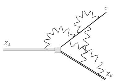
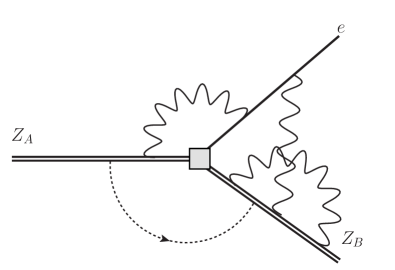
Figure 1: Examples of graphs in the dynamic subset (left) and the static subset (right). Heavy fields are drawn with double lines, while light fields (i.e. an electron) are drawn as single lines. The weak-current vertex is shown as a grey square (the neutrino is not drawn as it is electrically neutral). The photon drawn as a dashed line on the right causes the graph to vanish in Coulomb gauge.

Let us consider an amplitude computed using the Feynman rules of Eq. 10. We will group dynamically dressed graphs together and then add and subtract the wavefunction renormalization for the charge $z$ heavy particle order-by-order in perturbation theory. An example of a graph from this subset is shown on the left of Fig. 1. This subset of diagrams, which we will refer to as the “dynamic subset” is precisely equivalent to $\mathcal{M}_{\rm bkg}$ order-by-order in perturbation theory and therefore gauge invariant. The remaining diagrams, with the contribution from wavefunction renormalization subtracted, then form a separate gauge invariant class. These diagrams involve dressings of the heavy particles by photons (e.g. vertex corrections, self energies etc.). Since we work in the static limit, we refer to this set of diagrams as being the “static subset”. An example of a graph in the static subset is shown on the right of Fig. 1. Since the sum of both subsets is gauge invariant, and the dynamic subset is gauge invariant, it follows that the static subset is separately gauge invariant.

We now evaluate the static subset in Coulomb gauge (see Appendix B for a discussion). All diagrams contain either heavy-particle wavefunction renormalization, or heavy-heavy vertex corrections and these vanish diagram-by-diagram in Coulomb gauge. Since the static subset is gauge invariant, this statement is true for the sum of all diagrams for arbitrary gauge. Therefore, an amplitude computed with Eq. 10 agrees order by order in perturbation theory with an amplitude computed using Eq. 18.

Appendix B Coulomb gauge & the static limit

Let us work in the static limit $v=v^{\prime}$. We may then work in Coulomb gauge choosing $v_{\mu}=(1,0,0,0)$ such that transverse photons explicitly decouple from the heavy particles and Coulomb propagators, $D_{00}={\rm i}/\mathbf{q}^{2}$, contain no energetic poles. For a heavy particle in the initial and final state any sub-graph involving a photon which connects two heavy particle lines will result in an integrand with all of its poles on one side of the complex plane. The contour can then be closed in the opposite direction, and the integral will vanish. For example, let us take the following loop graph

$$\vspace{3pt}\raisebox{-25.0pt}{ \fmffile{new-name} \fmfgraph*(75,45) \fmfbottom{i1,o1} \fmftop{t1} \fmf{double}{i1,vl,t1} \fmf{dbl_dashes}{t1,vr,o1} \fmf{photon,tension=0}{vl,vr} \fmfv{d.sh=square,d.si=3mm}{t1} }\quad=\quad\int\frac{\differential^{d}L}{(2\pi)^{d}}\quantity(\frac{1}{L_{0}+{\rm i}0})^{2}\frac{{\rm i}}{\mathbf{L}^{2}}\quad=\quad 0~{}.\vspace{3pt}$$ (20)

A corollary of Eq. 20, and the fact that the heavy particle self-energies also vanish in Coulomb gauge, is the well known fact that the cusp anomalous dimension vanishes at zero recoil Grozin (2022).

This result also holds in the presence of dynamical fermions. Fermion loops can be performed first and do not mix longitudinal and transverse modes. As a result any graph containing a photon connecting two heavy lines will vanish. The only remaining graphs which are non-vanishing are ladder graphs, and ladder graphs dressed by sub-graphs on the electron lines. As discussed above these can be combined into the dynamic subset, and after adding wavefunction renormalization for heavy particle with charge $z$, form a gauge invariant subset. They may then be evaluated separately in whatever gauge is most convenient.

References

- Korchemsky and Radyushkin (1992) G. P. Korchemsky and A. V. Radyushkin, Phys. Lett. B 279, 359 (1992), eprint hep-ph/9203222.
- Isgur and Wise (1989) N. Isgur and M. B. Wise, Phys. Lett. B 232, 113 (1989).
- Isgur and Wise (1990) N. Isgur and M. B. Wise, Phys. Lett. B 237, 527 (1990).
- Georgi (1990) H. Georgi, Phys. Lett. B 240, 447 (1990).
- Falk et al. (1990) A. F. Falk, H. Georgi, B. Grinstein, and M. B. Wise, Nucl. Phys. B 343, 1 (1990).
- Bauer et al. (2002) C. W. Bauer, S. Fleming, D. Pirjol, I. Z. Rothstein, and I. W. Stewart, Phys. Rev. D 66, 014017 (2002), eprint hep-ph/0202088.
- Becher and Neubert (2009) T. Becher and M. Neubert, JHEP 06, 081 (2009), [Erratum: JHEP 11, 024 (2013)], eprint 0903.1126.
- Collins et al. (1989) J. C. Collins, D. E. Soper, and G. F. Sterman, Adv. Ser. Direct. High Energy Phys. 5, 1 (1989), eprint hep-ph/0409313.
- Grozin (2022) A. Grozin (2022), eprint 2212.05290.
- Yennie et al. (1961) D. R. Yennie, S. C. Frautschi, and H. Suura, Annals Phys. 13, 379 (1961).
- Gribov and Lipatov (1972) V. N. Gribov and L. N. Lipatov, Sov. J. Nucl. Phys. 15, 438 (1972).
- Altarelli and Parisi (1977) G. Altarelli and G. Parisi, Nucl. Phys. B 126, 298 (1977).
- Dokshitzer (1977) Y. L. Dokshitzer, Sov. Phys. JETP 46, 641 (1977).
- Brodsky (1971) S. J. Brodsky (1971), URL https://www.slac.stanford.edu/pubs/slacpubs/1000/slac-pub-1010.pdf.
- Neghabian and Gloeckle (1983) A. R. Neghabian and W. Gloeckle, Can. J. Phys. 61, 85 (1983).
- Weinberg (2005) S. Weinberg, The Quantum theory of fields. Vol. 1: Foundations. Chapter 13.6 (Cambridge University Press, 2005), ISBN 978-0-521-67053-1, 978-0-511-25204-4.
- Hardy and Towner (2020) J. C. Hardy and I. S. Towner, Phys. Rev. C 102, 045501 (2020).
- Branca et al. (2021) A. Branca, G. Brunetti, A. Longhin, M. Martini, F. Pupilli, and F. Terranova, Symmetry 13, 1625 (2021), eprint 2108.12212.
- Tomalak et al. (2022) O. Tomalak, Q. Chen, R. J. Hill, K. S. McFarland, and C. Wret, Phys. Rev. D 106, 093006 (2022), eprint 2204.11379.
- Seng et al. (2018) C.-Y. Seng, M. Gorchtein, H. H. Patel, and M. J. Ramsey-Musolf, Phys. Rev. Lett. 121, 241804 (2018), eprint 1807.10197.
- Czarnecki et al. (2019) A. Czarnecki, W. J. Marciano, and A. Sirlin, Phys. Rev. D 100, 073008 (2019), eprint 1907.06737.
- Dolinski et al. (2019) M. J. Dolinski, A. W. P. Poon, and W. Rodejohann, Ann. Rev. Nucl. Part. Sci. 69, 219 (2019), eprint 1902.04097.
- Jaus and Rasche (1970) W. Jaus and G. Rasche, Nucl. Phys. A 143, 202 (1970).
- Jaus (1972) W. Jaus, Phys. Lett. B 40, 616 (1972).
- Sirlin and Zucchini (1986) A. Sirlin and R. Zucchini, Phys. Rev. Lett. 57, 1994 (1986).
- Sirlin (1987) A. Sirlin, Phys. Rev. D 35, 3423 (1987).
- Weinberg (1965) S. Weinberg, Phys. Rev. 140, B516 (1965).
- Dittrich (1970) W. Dittrich, Phys. Rev. D 1, 3345 (1970).
- Szafron (2023) R. Szafron (2023), private communication.
- Borah et al. (2024) K. Borah, R. J. Hill, and R. Plestid (2024), eprint 2402.13307.
- Jaus and Rasche (1987) W. Jaus and G. Rasche, Phys. Rev. D 35, 3420 (1987).
- Beneke and Smirnov (1998) M. Beneke and V. A. Smirnov, Nucl. Phys. B 522, 321 (1998), eprint hep-ph/9711391.
- Jantzen (2011) B. Jantzen, JHEP 12, 076 (2011), eprint 1111.2589.
- Hill and Plestid (2023) R. J. Hill and R. Plestid (2023), eprint 2309.07343.