Functional Spatial Autoregressive Models

Tadao Hoshino School of Political Science and Economics, Waseda University, 1-6-1 Nishi-waseda, Shinjuku-ku, Tokyo 169-8050, Japan. Email: thoshino@waseda.jp.
Abstract

This study introduces a novel spatial autoregressive model in which the dependent variable is a function that may exhibit functional autocorrelation with the outcome functions of nearby units. This model can be characterized as a simultaneous integral equation system, which, in general, does not necessarily have a unique solution. For this issue, we provide a simple condition on the magnitude of the spatial interaction to ensure the uniqueness in data realization. For estimation, to account for the endogeneity caused by the spatial interaction, we propose a regularized two-stage least squares estimator based on a basis approximation for the functional parameter. The asymptotic properties of the estimator including the consistency and asymptotic normality are investigated under certain conditions. Additionally, we propose a simple Wald-type test for detecting the presence of spatial effects. As an empirical illustration, we apply the proposed model and method to analyze age distributions in Japanese cities.

Introduction

Spatial interdependence among units is a crucial element in spatial data analysis. To incorporate spatial interactions into econometric analysis, researchers have extensively utilized the Spatial Auto-Regressive (SAR) model:

yi=α0j=1nwi,jyj+xiβ0+εi,subscript𝑦𝑖subscript𝛼0superscriptsubscript𝑗1𝑛subscript𝑤𝑖𝑗subscript𝑦𝑗superscriptsubscript𝑥𝑖topsubscript𝛽0subscript𝜀𝑖\displaystyle y_{i}=\alpha_{0}\sum_{j=1}^{n}w_{i,j}y_{j}+x_{i}^{\top}\beta_{0}+\varepsilon_{i}, (1.1)

where yisubscript𝑦𝑖y_{i} denotes a scalar outcome, wi,jsubscript𝑤𝑖𝑗w_{i,j} denotes a known spatial weight between i𝑖i and j𝑗j, xisubscript𝑥𝑖x_{i} denotes a vector of explanatory variables, and εisubscript𝜀𝑖\varepsilon_{i} denotes an error term. The spatial lag term j=1nwi,jyjsuperscriptsubscript𝑗1𝑛subscript𝑤𝑖𝑗subscript𝑦𝑗\sum_{j=1}^{n}w_{i,j}y_{j} captures the spatial trend of the outcome variable in the neighborhood of i𝑖i, and the scalar parameter α0subscript𝛼0\alpha_{0} measures its impact. The usefulness of SAR modelling (1.1) has been demonstrated in various empirical topics, including regional economics, local politics, real estate, crimes, etc. In addition, if we define the weight term wi,jsubscript𝑤𝑖𝑗w_{i,j} based on social distance or friendship connections instead of geographic distance, then the SAR models can be utilized to analyze social network data, and their applicability is vast.

To further broaden the applications of SAR modelling, this study aims to extend (1.1) to a functional SAR model where the dependent variable is a function defined on the common support [0,1]01[0,1]:

qi(s)=j=1nwi,j01qj(t)α0(t,s)dt+xiβ0(s)+εi(s),fors[0,1],formulae-sequencesubscript𝑞𝑖𝑠superscriptsubscript𝑗1𝑛subscript𝑤𝑖𝑗superscriptsubscript01subscript𝑞𝑗𝑡subscript𝛼0𝑡𝑠d𝑡superscriptsubscript𝑥𝑖topsubscript𝛽0𝑠subscript𝜀𝑖𝑠for𝑠01\displaystyle q_{i}(s)=\sum_{j=1}^{n}w_{i,j}\int_{0}^{1}q_{j}(t)\alpha_{0}(t,s)\text{d}t+x_{i}^{\top}\beta_{0}(s)+\varepsilon_{i}(s),\;\;\text{for}\;\;s\in[0,1], (1.2)

where qi:[0,1]:subscript𝑞𝑖01q_{i}:[0,1]\to\mathbb{R} denotes the outcome function of interest. In particular, for empirical relevance, this study primarily focuses on the case in which qisubscript𝑞𝑖q_{i} is the quantile function for a scalar dependent variable of interest. Regression models involving functional variables have been widely studied in the literature of functional data analysis (FDA) for several decades (e.g., Ramsay and Silverman, 2005). Our model is essentially different from the existing ones in that we explicitly consider the simultaneous spatial interactions of the outcome functions.

As a motivating example, suppose we intend to investigate the impact of a regional childcare subsidy program in a given city on the age distribution of the city. The policy is likely to attract households with young children from other regions to benefit from the subsidy. Additionally, if childcare facilities and schools need to be newly constructed, inflows of other age groups can also be anticipated as workers. To obtain a comprehensive picture of the shift in the age distribution owing to the subsidy program in its entirety, it would be natural to consider a regression model in which the dependent variable represents the age distribution of each city, such as the quantile function. Meanwhile, when the size of the young population in a given city is in an increasing trend (no matter the cause), which serves as a driver of economic growth of the city, this might also lead to an influx of working-age population into the surrounding regions owing to the spatial spillover of economic activities. The proposed functional SAR model (1.2) is able to account for such interdependency between the outcome functions of nearby spatial units.

In the literature, we are not the first to consider an SAR-type modelling in the functional regression context. Zhu et al. (2022) proposed a social network model similar to ours in a time-series setting, where the response variable is a function of time. They assumed that only concurrent interactions exist at each moment such that the past and future outcomes of others do not affect the present outcome. Consequently, when fixed at each time point, their model can be reduced to the standard SAR model in (1.1). In this regard, our model may be considered to be a generalization of theirs such that α0(t,s)0subscript𝛼0𝑡𝑠0\alpha_{0}(t,s)\neq 0 is allowed for ts𝑡𝑠t\neq s in general.

Another related modelling approach to ours is the SAR quantile regression (e.g., Su and Yang, 2011; Malikov et al., 2019; Xu et al., 2022). When qisubscript𝑞𝑖q_{i} represents a quantile function, our model and theirs are conceptually similar in that both approaches can examine the distributional effects of explanatory variables on the outcome and the spatial interaction of outcomes in a unified framework. However, a fundamental distinction lies in that we consider a model in which each unit has its own unique quantile function as the dependent variable. Consequently, we can explicitly allow for each specific quantile value of an outcome to interact with other quantiles of others’ outcomes. For instance, our model can investigate the impacts of median outcome of neighborhoods on a specific (say) 10 percentile value of own outcome.

Notice that our model (1.2) is characterized as a simultaneous integral equation system, and to the best of our best knowledge, this type of modelling has not been investigated in the econometrics literature. To construct a consistent estimator for our model, the model space should be restricted such that the realized qisubscript𝑞𝑖q_{i}’s are uniquely (in some sense) associated with the true parameters. We show that to establish this uniqueness property, as in the standard SAR model (cf. Kelejian and Prucha, 2010), the spatial effects α0subscript𝛼0\alpha_{0} must be bounded within a certain range. In particular, we demonstrate that the tightness of the bound required for α0subscript𝛼0\alpha_{0} depends on the smoothness of the outcome function.

To estimate the model parameters, we need to address the endogeneity issue arising from the simultaneous interaction among the outcome functions. Thus, we propose a regularized two-stage least squares (2SLS) estimator that is based on a series approximation of α0(,s)subscript𝛼0𝑠\alpha_{0}(\cdot,s) at each evaluation point s𝑠s. Under the availability of a sufficient number of instrumental variables (IVs) and regularity conditions, we prove that both the estimator for β0subscript𝛽0\beta_{0} and that for α0(t,s)subscript𝛼0𝑡𝑠\alpha_{0}(t,s) are consistent at certain convergence rates and asymptotically normally distributed. Additionally, we develop a Wald-type test for assessing the presence of any spatial effects at each s𝑠s. We show that the proposed test statistic asymptotically distributes as the standard normal after appropriate normalization. Furthermore, we discuss performing the estimation when the outcome functions are not fully observable on the entire interval [0,1]01[0,1], but are only discretely observed, which is typical in most empirical situations. Our proposed estimator relies on a simple interpolation method, and we derive a set of conditions under which the estimator can achieve the same asymptotic properties as the infeasible counterpart.

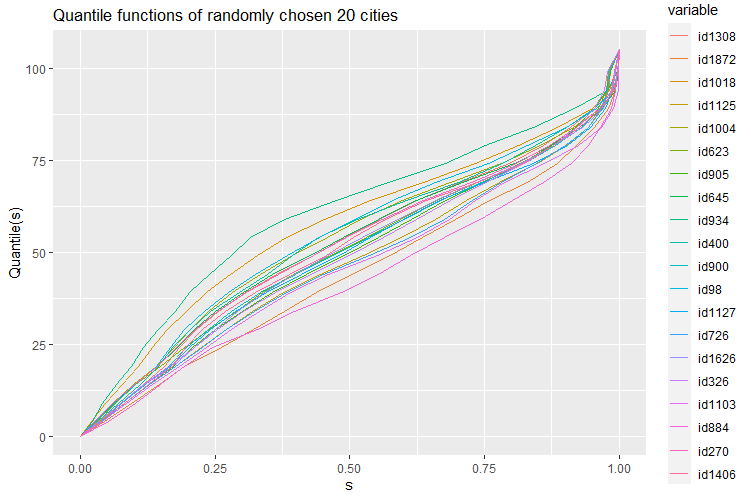
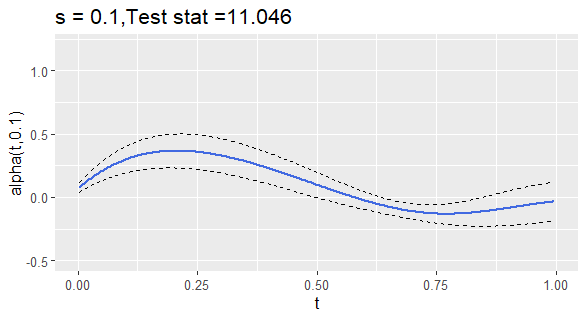
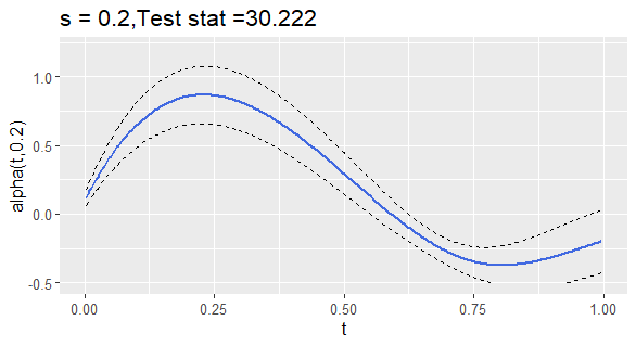
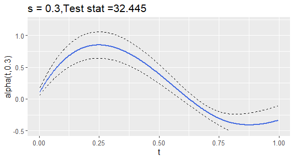
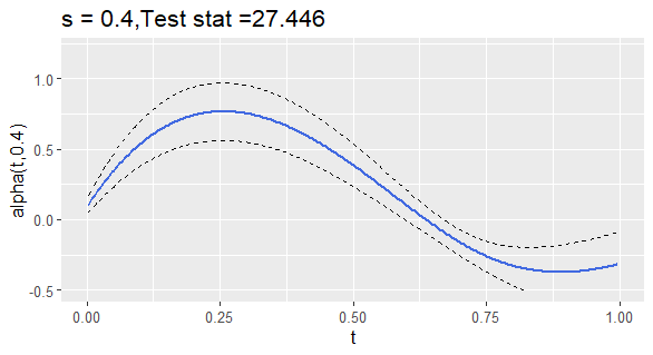
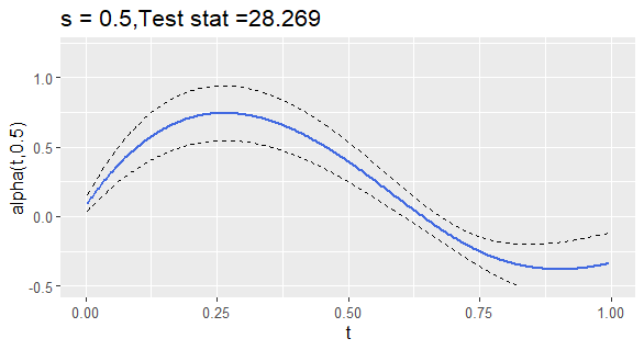
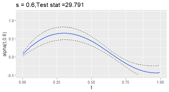
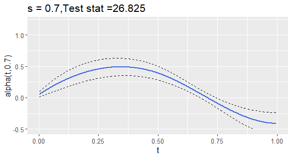
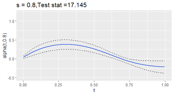
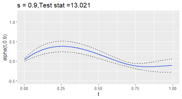
As an empirical illustration, we investigate the determinants of age distribution in Japanese cities. Since many Japanese cities are currently rapidly aging, which has emerged as one of the central social problems in the country, understanding the mechanisms underlying the age structure of cities is crucial. Using recent government survey data, including the Census, we apply our estimation and testing method to 1883 Japanese cities. Here, the outcome function qisubscript𝑞𝑖q_{i} represents the quantile function of the age distribution in city i𝑖i, and covariates xisubscript𝑥𝑖x_{i} include variables such as annual commercial sales, unemployment rate, number of childcare facilities, and others. Our results suggest that spatial interaction effects are extremely weak at quantiles close to the boundary points 0 or 1. This may not be surprising as all individuals are born at age 0 and have a life expectancy of approximately 100 years at maximum, resulting in little regional heterogeneity. In contrast, strong spatial effects are observed when both t𝑡t and s𝑠s are at approximately the ages of young working population, possibly indicating that economic activities and their spillovers are the main factors in shaping the spatial trend of age structure.

The remainder of this paper is organized as follows: In Section 2, we formally introduce the model proposed in this study and discuss the condition under which it is well defined with a unique solution. In addition, focusing on the cases where the outcome function is a quantile function, we discuss the motivations and interpretation of such a modelling approach. In Section 3, we describe our 2SLS method for estimating β0subscript𝛽0\beta_{0} and α0subscript𝛼0\alpha_{0}. Thereafter, we study the asymptotic properties of the proposed estimator under a set of assumptions. In this section, we also propose a test statistic for testing the null hypothesis that α0(t,s)=0subscript𝛼0𝑡𝑠0\alpha_{0}(t,s)=0 for t𝑡t\in\mathcal{I}, and its asymptotic distribution is derived. In Section 4, we present the results of Monte Carlo experiments to evaluate the finite sample performance of the proposed estimator and test. Section 5 presents our empirical analysis on the age distribution of Japanese cities, and Section 6 concludes the paper.

Notation

For a natural number n𝑛n, Insubscript𝐼𝑛I_{n} denotes an n×n𝑛𝑛n\times n identity matrix. For a function hh defined on [0,1]01[0,1], the Lpsuperscript𝐿𝑝L^{p} norm of hh is written as hLp(01|h(s)|pds)1/psubscriptnormsuperscript𝐿𝑝superscriptsuperscriptsubscript01superscript𝑠𝑝d𝑠1𝑝||h||_{L^{p}}\coloneqq(\int_{0}^{1}|h(s)|^{p}\text{d}s)^{1/p}, and Lp(0,1)superscript𝐿𝑝01L^{p}(0,1) denotes the set of hh’s such that hLp<subscriptnormsuperscript𝐿𝑝||h||_{L^{p}}<\infty. For a random variable x𝑥x, the Lpsuperscript𝐿𝑝L^{p} norm of x𝑥x is written as xp(𝔼|x|p)1/psubscriptnorm𝑥𝑝superscript𝔼superscript𝑥𝑝1𝑝||x||_{p}\coloneqq(\mathbb{E}|x|^{p})^{1/p}. For a matrix A𝐴A, Anorm𝐴||A|| and Asubscriptnorm𝐴||A||_{\infty} denote the Frobenius norm and the maximum absolute row sum of A𝐴A, respectively. If A𝐴A is a square matrix, we use ρmax(A)subscript𝜌𝐴\rho_{\max}(A) and ρmin(A)subscript𝜌𝐴\rho_{\min}(A) to denote its largest and smallest eigenvalues, respectively. In addition, Asuperscript𝐴A^{-} is a symmetric generalized inverse of A𝐴A. We write abless-than-or-similar-to𝑎𝑏a\lesssim b and apbsubscriptless-than-or-similar-to𝑝𝑎𝑏a\lesssim_{p}b if a=O(b)𝑎𝑂𝑏a=O(b) and a=OP(b)𝑎subscript𝑂𝑃𝑏a=O_{P}(b), respectively. Finally, we write absimilar-to𝑎𝑏a\sim b when abless-than-or-similar-to𝑎𝑏a\lesssim b and baless-than-or-similar-to𝑏𝑎b\lesssim a.

Functional SAR Models

Model Setup and Completeness

Suppose that we have data of size n𝑛n: {(qi,xi,wi,1,,wi,n)}i=1nsuperscriptsubscriptsubscript𝑞𝑖subscript𝑥𝑖subscript𝑤𝑖1subscript𝑤𝑖𝑛𝑖1𝑛\{(q_{i},x_{i},w_{i,1},\ldots,w_{i,n})\}_{i=1}^{n}, where qisubscript𝑞𝑖q_{i} denotes a random outcome function of interest with the common support [0,1]01[0,1], xi=(xi,1,,xi,dx)dxsubscript𝑥𝑖superscriptsubscript𝑥𝑖1subscript𝑥𝑖subscript𝑑𝑥topsuperscriptsubscript𝑑𝑥x_{i}=(x_{i,1},\ldots,x_{i,d_{x}})^{\top}\in\mathbb{R}^{d_{x}} denotes a vector of covariates including a constant term, and wi,jsubscript𝑤𝑖𝑗w_{i,j}\in\mathbb{R} denotes the (i,j)𝑖𝑗(i,j)-th element of an n×n𝑛𝑛n\times n pre-specified spatial weight matrix Wn=(wi,j)i,j=1nsubscript𝑊𝑛superscriptsubscriptsubscript𝑤𝑖𝑗𝑖𝑗1𝑛W_{n}=(w_{i,j})_{i,j=1}^{n}. The value of each wi,jsubscript𝑤𝑖𝑗w_{i,j} is determined non-randomly. As is the convention, we set wi,i=0subscript𝑤𝑖𝑖0w_{i,i}=0 for all i𝑖i for normalization. Note that the spatial configurations of the units generally change with the sample size. Thus, the variables generally form triangular arrays, and model parameters depend on n𝑛n through spatial interactions. However, when there is no confusion, the dependence on n𝑛n is suppressed for notational convenience.

As shown in (1.2), our working model is

qi(s)=01q¯i(t)α0(t,s)dt+xiβ0(s)+εi(s),fors[0,1],formulae-sequencesubscript𝑞𝑖𝑠superscriptsubscript01subscript¯𝑞𝑖𝑡subscript𝛼0𝑡𝑠d𝑡superscriptsubscript𝑥𝑖topsubscript𝛽0𝑠subscript𝜀𝑖𝑠for𝑠01\displaystyle q_{i}(s)=\int_{0}^{1}\overline{q}_{i}(t)\alpha_{0}(t,s)\text{d}t+x_{i}^{\top}\beta_{0}(s)+\varepsilon_{i}(s),\;\;\text{for}\;\;s\in[0,1], (2.1)

where q¯isubscript¯𝑞𝑖\overline{q}_{i} denotes the spatial lag of the outcome function: q¯ij=1nwi,jqjsubscript¯𝑞𝑖superscriptsubscript𝑗1𝑛subscript𝑤𝑖𝑗subscript𝑞𝑗\overline{q}_{i}\coloneqq\sum_{j=1}^{n}w_{i,j}q_{j}. The unknown parameters to be estimated are α0subscript𝛼0\alpha_{0} and β0=(β01,,β0dx)subscript𝛽0superscriptsubscript𝛽01subscript𝛽0subscript𝑑𝑥top\beta_{0}=(\beta_{01},\ldots,\beta_{0d_{x}})^{\top}. For instance, in our empirical analysis, qi(s)subscript𝑞𝑖𝑠q_{i}(s) denotes the s𝑠s-th quantile of the age distribution in city i𝑖i, and α0(t,s)subscript𝛼0𝑡𝑠\alpha_{0}(t,s) captures the impacts from the t𝑡t-th quantile ages of neighborhood cities to the s𝑠s-th quantile age of own city. For other examples, qi(s)subscript𝑞𝑖𝑠q_{i}(s) could be the s𝑠s-th quantile of the income distribution in city i𝑖i, s𝑠s-th quantile of the daily activity energy expenditure of person i𝑖i, number of available bicycles at the bicycle-sharing station i𝑖i at time s𝑠s, and so forth. Hereinafter, we assume that qiLp(0,1)subscript𝑞𝑖superscript𝐿𝑝01q_{i}\in L^{p}(0,1) for some 2p<2𝑝2\leq p<\infty and that α0C[0,1]2subscript𝛼0𝐶superscript012\alpha_{0}\in C[0,1]^{2}, where C[0,1]2𝐶superscript012C[0,1]^{2} denotes the set of continuous functions on [0,1]2superscript012[0,1]^{2}.


Before turning to the estimation of α0subscript𝛼0\alpha_{0} and β0subscript𝛽0\beta_{0}, we discuss the completeness of our model, that is, whether model (1.2) can be characterized by a unique solution (q1,,qn)subscript𝑞1subscript𝑞𝑛(q_{1},\ldots,q_{n}). As our model comprises a system of n𝑛n functional equations, the existence and uniqueness of the solution are non-trivial problems. If the system does not have or has multiple solutions, consistently estimating the model parameters without some ad hoc assumptions is generally impossible.

Let Q(s)=(q1(s),,qn(s))𝑄𝑠superscriptsubscript𝑞1𝑠subscript𝑞𝑛𝑠topQ(s)=(q_{1}(s),\ldots,q_{n}(s))^{\top}, X=(x1,,xn)𝑋superscriptsubscript𝑥1subscript𝑥𝑛topX=(x_{1},\ldots,x_{n})^{\top}, and (s)=(ε1(s),,εn(s))𝑠superscriptsubscript𝜀1𝑠subscript𝜀𝑛𝑠top\mathcal{E}(s)=(\varepsilon_{1}(s),\ldots,\varepsilon_{n}(s))^{\top}. Then, we can re-write (1.2) in matrix form as

Q(s)=Wn01Q(t)α0(t,s)dt+Xβ0(s)+(s).𝑄𝑠subscript𝑊𝑛superscriptsubscript01𝑄𝑡subscript𝛼0𝑡𝑠d𝑡𝑋subscript𝛽0𝑠𝑠\displaystyle Q(s)=W_{n}\int_{0}^{1}Q(t)\alpha_{0}(t,s)\text{d}t+X\beta_{0}(s)+\mathcal{E}(s). (2.2)

This expression suggests that our model is seen as a system of Fredholm integral equations of the second kind with kernel α0(t,s)subscript𝛼0𝑡𝑠\alpha_{0}(t,s). Defining α¯0max(t,s)[0,1]2|α0(t,s)|subscript¯𝛼0subscript𝑡𝑠superscript012subscript𝛼0𝑡𝑠\overline{\alpha}_{0}\coloneqq\max_{(t,s)\in[0,1]^{2}}|\alpha_{0}(t,s)|, whose existence is ensured under the continuity of α0subscript𝛼0\alpha_{0}, assume the following:

Assumption 2.1.

α¯01less-than-or-similar-tosubscript¯𝛼01\overline{\alpha}_{0}\lesssim 1 and Wn1less-than-or-similar-tosubscriptnormsubscript𝑊𝑛1||W_{n}||_{\infty}\lesssim 1 such that α¯0Wn<1subscript¯𝛼0subscriptnormsubscript𝑊𝑛1\overline{\alpha}_{0}||W_{n}||_{\infty}<1.

Let n,p{H=(h1,,hn):hiLp(0,1)for alli}subscript𝑛𝑝conditional-set𝐻subscript1subscript𝑛subscript𝑖superscript𝐿𝑝01for all𝑖\mathcal{H}_{n,p}\coloneqq\{H=(h_{1},\ldots,h_{n}):h_{i}\in L^{p}(0,1)\;\text{for all}\;i\}, and define a linear operator 𝒯𝒯\mathcal{T} as

(𝒯H)(s)Wn01H(t)α0(t,s)dt𝒯𝐻𝑠subscript𝑊𝑛superscriptsubscript01𝐻𝑡subscript𝛼0𝑡𝑠d𝑡\displaystyle(\mathcal{T}H)(s)\coloneqq W_{n}\int_{0}^{1}H(t)\alpha_{0}(t,s)\text{d}t (2.3)

for Hn,p𝐻subscript𝑛𝑝H\in\mathcal{H}_{n,p}, whose range is n,psubscript𝑛𝑝\mathcal{H}_{n,p} under Assumption 2.1. Thus, we can write Q=𝒯Q+Xβ0+𝑄𝒯𝑄𝑋subscript𝛽0Q=\mathcal{T}Q+X\beta_{0}+\mathcal{E}. Then, denoting Id to be the identity operator, if the inverse operator (Id𝒯)1superscriptId𝒯1(\text{Id}-\mathcal{T})^{-1} exists, the solution Q𝑄Q of the system can be uniquely determined (as an element of n,psubscript𝑛𝑝\mathcal{H}_{n,p}) as Q=(Id𝒯)1[Xβ0+]𝑄superscriptId𝒯1delimited-[]𝑋subscript𝛽0Q=(\text{Id}-\mathcal{T})^{-1}[X\beta_{0}+\mathcal{E}].

The next proposition states that Assumption 2.1 is sufficient for the existence of (Id𝒯)1superscriptId𝒯1(\text{Id}-\mathcal{T})^{-1} and uniqueness of Q𝑄Q.

Proposition 2.1.

Suppose that Assumption 2.1 holds. Then, (Id𝒯)1superscriptId𝒯1(\text{Id}-\mathcal{T})^{-1} exists, and Q𝑄Q is the only solution of (1.2) in the Banach space (n,p,||||,p)(\mathcal{H}_{n,p},||\cdot||_{\infty,p}), where H,pmax1inhiLpsubscriptnorm𝐻𝑝subscript1𝑖𝑛subscriptnormsubscript𝑖superscript𝐿𝑝||H||_{\infty,p}\coloneqq\max_{1\leq i\leq n}||h_{i}||_{L^{p}}.

The proof is straightforward. Under Assumption 2.1, we have

{𝒯H}iLp=j=1nwi,j01hj(t)α0(t,)dtLpj=1n|wi,j|(01|01hj(t)α0(t,s)dt|pds)1/pj=1n|wi,j|(0101|hj(t)|p|α0(t,s)|pdtds)1/pα¯0Wnmax1jnhjLp<H,p<subscriptdelimited-∥∥subscript𝒯𝐻𝑖superscript𝐿𝑝subscriptdelimited-∥∥superscriptsubscript𝑗1𝑛subscript𝑤𝑖𝑗superscriptsubscript01subscript𝑗𝑡subscript𝛼0𝑡d𝑡superscript𝐿𝑝superscriptsubscript𝑗1𝑛subscript𝑤𝑖𝑗superscriptsuperscriptsubscript01superscriptsuperscriptsubscript01subscript𝑗𝑡subscript𝛼0𝑡𝑠d𝑡𝑝d𝑠1𝑝superscriptsubscript𝑗1𝑛subscript𝑤𝑖𝑗superscriptsuperscriptsubscript01superscriptsubscript01superscriptsubscript𝑗𝑡𝑝superscriptsubscript𝛼0𝑡𝑠𝑝d𝑡d𝑠1𝑝subscript¯𝛼0subscriptnormsubscript𝑊𝑛subscript1𝑗𝑛subscriptnormsubscript𝑗superscript𝐿𝑝subscriptnorm𝐻𝑝\displaystyle\begin{split}\left\|\{\mathcal{T}H\}_{i}\right\|_{L^{p}}=\left\|\sum_{j=1}^{n}w_{i,j}\int_{0}^{1}h_{j}(t)\alpha_{0}(t,\cdot)\text{d}t\right\|_{L^{p}}&\leq\sum_{j=1}^{n}|w_{i,j}|\left(\int_{0}^{1}\left|\int_{0}^{1}h_{j}(t)\alpha_{0}(t,s)\text{d}t\right|^{p}\text{d}s\right)^{1/p}\\ &\leq\sum_{j=1}^{n}|w_{i,j}|\left(\int_{0}^{1}\int_{0}^{1}\left|h_{j}(t)\right|^{p}\left|\alpha_{0}(t,s)\right|^{p}\text{d}t\text{d}s\right)^{1/p}\\ &\leq\overline{\alpha}_{0}||W_{n}||_{\infty}\max_{1\leq j\leq n}||h_{j}||_{L^{p}}<||H||_{\infty,p}<\infty\end{split} (2.4)

for any Hn,p𝐻subscript𝑛𝑝H\in\mathcal{H}_{n,p} by Minkowski’s and Jensen’s inequalities. This implies that 𝒯Hn,p𝒯𝐻subscript𝑛𝑝\mathcal{T}H\in\mathcal{H}_{n,p}. As is well known, if the operator norm of 𝒯𝒯\mathcal{T} is smaller than one, (Id𝒯)1superscriptId𝒯1(\text{Id}-\mathcal{T})^{-1} exists, and we have the Neumann series expansion (Id𝒯)1==0𝒯superscriptId𝒯1superscriptsubscript0superscript𝒯(\text{Id}-\mathcal{T})^{-1}=\sum_{\ell=0}^{\infty}\mathcal{T}^{\ell} converging in the operator norm (e.g., Theorem 2.14, Kress (2014)). It is immediate from (2.4) that 𝒯H,p<1subscriptnorm𝒯𝐻𝑝1\left\|\mathcal{T}H\right\|_{\infty,p}<1 follows for any H𝐻H such that H,p=1subscriptnorm𝐻𝑝1||H||_{\infty,p}=1, which yields the desired result.


When the spatial weight matrix is row-normalized such that Wn=1subscriptnormsubscript𝑊𝑛1||W_{n}||_{\infty}=1, as is often the case in empirical applications, Assumption 2.1 can be reduced to α¯0<1subscript¯𝛼01\overline{\alpha}_{0}<1, which somewhat resembles the solvability condition |α0|<1subscript𝛼01|\alpha_{0}|<1 for the standard linear SAR model (1.1).

Remark 2.1 (Alternative condition).

If one imposes a stronger assumption on the space of the input functions, the requirement for the kernel can be relaxed. For example, for all i𝑖i, suppose that qisubscript𝑞𝑖q_{i} belongs to C[0,1]𝐶01C[0,1]. Then, by the extreme value theorem, qisubscript𝑞𝑖q_{i}’s are bounded. Letting n,{H=(h1,,hn):hiC[0,1]for alli}subscript𝑛conditional-set𝐻subscript1subscript𝑛subscript𝑖𝐶01for all𝑖\mathcal{H}_{n,\infty}\coloneqq\{H=(h_{1},\ldots,h_{n}):h_{i}\in C[0,1]\;\text{for all}\;i\} and H,max1inmaxs[0,1]|hi(s)|subscriptnorm𝐻subscript1𝑖𝑛subscript𝑠01subscript𝑖𝑠||H||_{\infty,\infty}\coloneqq\max_{1\leq i\leq n}\max_{s\in[0,1]}|h_{i}(s)|, we can easily show that Q𝑄Q is the only solution in the Banach space (n,,||||,)(\mathcal{H}_{n,\infty},||\cdot||_{\infty,\infty}) if Wnmaxs[0,1]01|α0(t,s)|dt<1subscriptnormsubscript𝑊𝑛subscript𝑠01superscriptsubscript01subscript𝛼0𝑡𝑠d𝑡1||W_{n}||_{\infty}\max_{s\in[0,1]}\int_{0}^{1}|\alpha_{0}(t,s)|\text{d}t<1 is satisfied.111 Clearly, for any given Hn,𝐻subscript𝑛H\in\mathcal{H}_{n,\infty} such that H,=1subscriptnorm𝐻1||H||_{\infty,\infty}=1, we have |{(𝒯H)(s)}i|j=1n|wi,j|01|hj(t)||α0(t,s)|dtWnmaxs[0,1]01|α0(t,s)|dt.subscript𝒯𝐻𝑠𝑖superscriptsubscript𝑗1𝑛subscript𝑤𝑖𝑗superscriptsubscript01subscript𝑗𝑡subscript𝛼0𝑡𝑠d𝑡subscriptnormsubscript𝑊𝑛subscript𝑠01superscriptsubscript01subscript𝛼0𝑡𝑠d𝑡\displaystyle\left|\{(\mathcal{T}H)(s)\}_{i}\right|\leq\sum_{j=1}^{n}|w_{i,j}|\int_{0}^{1}|h_{j}(t)|\cdot|\alpha_{0}(t,s)|\text{d}t\leq||W_{n}||_{\infty}\max_{s\in[0,1]}\int_{0}^{1}|\alpha_{0}(t,s)|\text{d}t. If the spatial weight matrix is row-normalized, then the condition can be further simplified to maxs[0,1]01|α0(t,s)|dt<1subscript𝑠01superscriptsubscript01subscript𝛼0𝑡𝑠d𝑡1\max_{s\in[0,1]}\int_{0}^{1}|\alpha_{0}(t,s)|\text{d}t<1, which is a familiar requirement for the solvability of the Fredholm integral equation of the second kind (e.g., Corollary 2.16, Kress (2014)). It is known that compactly supported continuous functions are dense in Lpsuperscript𝐿𝑝L^{p} (1p<1𝑝1\leq p<\infty). Thus, in practice, assuming that all qisubscript𝑞𝑖q_{i}’s are continuous is almost harmless, and hence the violation of Assumption 2.1 should be allowed to some extent.

The Neumann series expansion implies that Q𝑄Q can be expressed as Q=Xβ0+𝒯Xβ0+𝒯2Xβ0+++𝒯+𝒯2+𝑄𝑋subscript𝛽0𝒯𝑋subscript𝛽0superscript𝒯2𝑋subscript𝛽0𝒯superscript𝒯2Q=X\beta_{0}+\mathcal{T}X\beta_{0}+\mathcal{T}^{2}X\beta_{0}+\cdots+\mathcal{E}+\mathcal{T}\mathcal{E}+\mathcal{T}^{2}\mathcal{E}+\cdots, that is,

Q()𝑄\displaystyle Q(\cdot) =Xβ0()+WnX01β0(t)α0(t,)dt+WnWnX0101β0(t1)α0(t1,t2)α0(t2,)dt1dt2+absent𝑋subscript𝛽0subscript𝑊𝑛𝑋superscriptsubscript01subscript𝛽0𝑡subscript𝛼0𝑡d𝑡subscript𝑊𝑛subscript𝑊𝑛𝑋superscriptsubscript01superscriptsubscript01subscript𝛽0subscript𝑡1subscript𝛼0subscript𝑡1subscript𝑡2subscript𝛼0subscript𝑡2dsubscript𝑡1dsubscript𝑡2\displaystyle=X\beta_{0}(\cdot)+W_{n}X\int_{0}^{1}\beta_{0}(t)\alpha_{0}(t,\cdot)\text{d}t+W_{n}W_{n}X\int_{0}^{1}\int_{0}^{1}\beta_{0}(t_{1})\alpha_{0}(t_{1},t_{2})\alpha_{0}(t_{2},\cdot)\text{d}t_{1}\text{d}t_{2}+\cdots (2.5)

Hence, the marginal effect of increasing xi,jsubscript𝑥𝑖𝑗x_{i,j} on Q()𝑄Q(\cdot) is obtained by

Q()xi,j𝑄subscript𝑥𝑖𝑗\displaystyle\frac{\partial Q(\cdot)}{\partial x_{i,j}} =𝒆iβ0j()+Wn𝒆i01β0j(t)α0(t,)dt+WnWn𝒆i0101β0j(t1)α0(t1,t2)α0(t2,)dt1dt2+,absentsubscript𝒆𝑖subscript𝛽0𝑗subscript𝑊𝑛subscript𝒆𝑖superscriptsubscript01subscript𝛽0𝑗𝑡subscript𝛼0𝑡d𝑡subscript𝑊𝑛subscript𝑊𝑛subscript𝒆𝑖superscriptsubscript01superscriptsubscript01subscript𝛽0𝑗subscript𝑡1subscript𝛼0subscript𝑡1subscript𝑡2subscript𝛼0subscript𝑡2dsubscript𝑡1dsubscript𝑡2\displaystyle=\bm{e}_{i}\beta_{0j}(\cdot)+W_{n}\bm{e}_{i}\int_{0}^{1}\beta_{0j}(t)\alpha_{0}(t,\cdot)\text{d}t+W_{n}W_{n}\bm{e}_{i}\int_{0}^{1}\int_{0}^{1}\beta_{0j}(t_{1})\alpha_{0}(t_{1},t_{2})\alpha_{0}(t_{2},\cdot)\text{d}t_{1}\text{d}t_{2}+\cdots, (2.6)

where 𝒆isubscript𝒆𝑖\bm{e}_{i} denotes the i𝑖i-th column of Insubscript𝐼𝑛I_{n}. This clearly shows that a change in i𝑖i’s covariate affects not only the outcome of i𝑖i but also those of other units through the spatial interaction - the so-called spatial multiplier effect.

Leading Example: A Distributional SAR Model

One of the situations in which model (1.2) can be most nicely applied empirically would be when the outcome function qisubscript𝑞𝑖q_{i} represents the quantile function for the cumulative distribution function (CDF) of a variable of interest. In our empirical analysis, we study the determinants of the population pyramids of Japanese cities by employing the age quantile function of city i𝑖i as qisubscript𝑞𝑖q_{i}.

Suppose that for each i𝑖i we can observe a random CDF Fisubscript𝐹𝑖F_{i} for an outcome variable y𝒴i𝑦subscript𝒴𝑖y\in\mathcal{Y}_{i}\subseteq\mathbb{R} of interest. The quantile function of y𝑦y for i𝑖i is defined as qi(s)inf{y𝒴i:sFi(y)}subscript𝑞𝑖𝑠infimumconditional-set𝑦subscript𝒴𝑖𝑠subscript𝐹𝑖𝑦q_{i}(s)\coloneqq\inf\{y\in\mathcal{Y}_{i}:s\leq F_{i}(y)\}. In the FDA literature, models where the response variable represents a probability distribution have garnered significant attention, for example, Petersen and Müller (2016), Han et al. (2020), Yang et al. (2020), Yang (2020), Ghodrati and Panaretos (2022), Petersen et al. (2021), Chen et al. (2023). For an excellent review on this topic, refer to Petersen et al. (2022). A common view in these studies is that performing a regression analysis directly in the space of CDFs (or densities) is often problematic. Hence, we should consider imposing a regression model on the quantile function (rather than on the CDF per se), as in Yang et al. (2020) and Yang (2020), enabling us to enjoy several analytically and interpretationally preferable properties as mentioned below.

First, quantile functions can be easily computed without considering the range boundaries, unlike CDFs. Second, the domains of CDFs are typically heterogeneous across individuals, whereas that of quantile functions is always the fixed interval [0,1]01[0,1]. Third, the least-squares regression of the quantile function can be nicely interpreted as a Wasserstein distance minimization problem.

More specifically for the third point, denoting Fiα,βsuperscriptsubscript𝐹𝑖𝛼𝛽F_{i}^{\alpha,\beta} to be the CDF induced from the quantile function qiα,β(s)01q¯i(t)α(t,s)dt+xiβ(s)superscriptsubscript𝑞𝑖𝛼𝛽𝑠superscriptsubscript01subscript¯𝑞𝑖𝑡𝛼𝑡𝑠d𝑡superscriptsubscript𝑥𝑖top𝛽𝑠q_{i}^{\alpha,\beta}(s)\coloneqq\int_{0}^{1}\overline{q}_{i}(t)\alpha(t,s)\text{d}t+x_{i}^{\top}\beta(s), the squared 222-Wasserstein distance between Fisubscript𝐹𝑖F_{i} and Fiα,βsuperscriptsubscript𝐹𝑖𝛼𝛽F_{i}^{\alpha,\beta} is obtained as222 Formally, the Wasserstein distance is a distance between two probability measures. We abuse the notation using CDFs in its arguments for ease of explanation. For more precise discussions on the properties of Wasserstein distance, see Panaretos and Zemel (2020), for instance.

𝒲22(Fi,Fiα,β)=01(qi(s)qiα,β(s))2ds.superscriptsubscript𝒲22subscript𝐹𝑖superscriptsubscript𝐹𝑖𝛼𝛽superscriptsubscript01superscriptsubscript𝑞𝑖𝑠superscriptsubscript𝑞𝑖𝛼𝛽𝑠2d𝑠\displaystyle\mathcal{W}_{2}^{2}(F_{i},F_{i}^{\alpha,\beta})=\int_{0}^{1}\left(q_{i}(s)-q_{i}^{\alpha,\beta}(s)\right)^{2}\text{d}s. (2.7)

Thus, minimizing the mean squared Wasserstein distance with respect to (α,β)𝛼𝛽(\alpha,\beta): minα,βn1i=1n𝒲22(Fi,Fiα,β)subscript𝛼𝛽superscript𝑛1superscriptsubscript𝑖1𝑛superscriptsubscript𝒲22subscript𝐹𝑖superscriptsubscript𝐹𝑖𝛼𝛽\min_{\alpha,\beta}n^{-1}\sum_{i=1}^{n}\mathcal{W}_{2}^{2}(F_{i},F_{i}^{\alpha,\beta}) is equivalent to performing a functional least squares regression based on model (1.2). Note, however, that the resulting least squares estimator does not produce a consistent estimate of (α0,β0)subscript𝛼0subscript𝛽0(\alpha_{0},\beta_{0}) because of the endogeneity of q¯isubscript¯𝑞𝑖\overline{q}_{i}. To circumvent the endogeneity issue, we introduce a penalized 2SLS method in the next section.

It is also worth noting that the spatially lagged quantile q¯isubscript¯𝑞𝑖\overline{q}_{i} corresponds to the quantile function of the spatially weighted Fréchet mean F¯isubscript¯𝐹𝑖\overline{F}_{i} of {F1,,Fn}subscript𝐹1subscript𝐹𝑛\{F_{1},\ldots,F_{n}\} at the location of i𝑖i: F¯iargminFj=1nwi,j𝒲22(F,Fj)subscript¯𝐹𝑖subscript𝐹superscriptsubscript𝑗1𝑛subscript𝑤𝑖𝑗superscriptsubscript𝒲22𝐹subscript𝐹𝑗\overline{F}_{i}\coloneqq\arg\min_{F}\sum_{j=1}^{n}w_{i,j}\mathcal{W}_{2}^{2}(F,F_{j}), which is also referred to as the Wasserstein barycenter, with wi,j0subscript𝑤𝑖𝑗0w_{i,j}\geq 0 and j=1nwi,j=1superscriptsubscript𝑗1𝑛subscript𝑤𝑖𝑗1\sum_{j=1}^{n}w_{i,j}=1. Rather than using q¯isubscript¯𝑞𝑖\overline{q}_{i}, one might consider employing the quantile function of the spatially lagged CDF: j=1nwi,jFisuperscriptsubscript𝑗1𝑛subscript𝑤𝑖𝑗subscript𝐹𝑖\sum_{j=1}^{n}w_{i,j}F_{i} as the spatial trend term. However, a linear mixture of CDFs is generally multimodal and does not inherit the shape properties of the original CDFs. In this regard, the weighted Fréchet mean should be more representative and faithful as an indicator of the neighborhood trend. This point is also highlighted in Gunsilius (2023) in the context of synthetic control analysis.

Estimation and Asymptotics

Penalized 2SLS estimator

We now discuss the estimation of α0subscript𝛼0\alpha_{0} and β0subscript𝛽0\beta_{0}. Let {ϕk:k=1,2,}conditional-setsubscriptitalic-ϕ𝑘𝑘12\{\phi_{k}:k=1,2,\ldots\} be a series of basis functions, such as Fourier series, B-splines, and wavelets, such that we can expand α0(t,s)=k=1ϕk(t)θ0k(s)subscript𝛼0𝑡𝑠superscriptsubscript𝑘1subscriptitalic-ϕ𝑘𝑡subscript𝜃0𝑘𝑠\alpha_{0}(t,s)=\sum_{k=1}^{\infty}\phi_{k}(t)\theta_{0k}(s) for each s𝑠s. Then, we have 01qi(t)α0(t,s)dt=k=1ri,kθ0k(s)superscriptsubscript01subscript𝑞𝑖𝑡subscript𝛼0𝑡𝑠d𝑡superscriptsubscript𝑘1subscript𝑟𝑖𝑘subscript𝜃0𝑘𝑠\int_{0}^{1}q_{i}(t)\alpha_{0}(t,s)\text{d}t=\sum_{k=1}^{\infty}r_{i,k}\theta_{0k}(s), where ri,k01qi(t)ϕk(t)dtsubscript𝑟𝑖𝑘superscriptsubscript01subscript𝑞𝑖𝑡subscriptitalic-ϕ𝑘𝑡d𝑡r_{i,k}\coloneqq\int_{0}^{1}q_{i}(t)\phi_{k}(t)\text{d}t. Hence, our model (1.2) can be re-written as

qi(s)subscript𝑞𝑖𝑠\displaystyle q_{i}(s) =k=1Kr¯i,kθ0k(s)+xiβ0(s)+εi(s)+ui(s)absentsuperscriptsubscript𝑘1𝐾subscript¯𝑟𝑖𝑘subscript𝜃0𝑘𝑠superscriptsubscript𝑥𝑖topsubscript𝛽0𝑠subscript𝜀𝑖𝑠subscript𝑢𝑖𝑠\displaystyle=\sum_{k=1}^{K}\overline{r}_{i,k}\theta_{0k}(s)+x_{i}^{\top}\beta_{0}(s)+\varepsilon_{i}(s)+u_{i}(s) (3.1)

where r¯i,kj=1nwi,jrj,ksubscript¯𝑟𝑖𝑘superscriptsubscript𝑗1𝑛subscript𝑤𝑖𝑗subscript𝑟𝑗𝑘\overline{r}_{i,k}\coloneqq\sum_{j=1}^{n}w_{i,j}r_{j,k}, ui(s)01q¯i(t)α0(t,s)dtk=1Kr¯i,kθ0k(s)subscript𝑢𝑖𝑠superscriptsubscript01subscript¯𝑞𝑖𝑡subscript𝛼0𝑡𝑠d𝑡superscriptsubscript𝑘1𝐾subscript¯𝑟𝑖𝑘subscript𝜃0𝑘𝑠u_{i}(s)\coloneqq\int_{0}^{1}\overline{q}_{i}(t)\alpha_{0}(t,s)\text{d}t-\sum_{k=1}^{K}\overline{r}_{i,k}\theta_{0k}(s), and KKn𝐾subscript𝐾𝑛K\equiv K_{n} is a sequence of integers tending to infinity as n𝑛n grows. Note that this is just a multiple regression model having K𝐾K endogenous regressors r¯i=(r¯i,1,,r¯i,K)subscript¯𝑟𝑖superscriptsubscript¯𝑟𝑖1subscript¯𝑟𝑖𝐾top\overline{r}_{i}=(\overline{r}_{i,1},\ldots,\overline{r}_{i,K})^{\top} with a composite error term εi(s)+ui(s)subscript𝜀𝑖𝑠subscript𝑢𝑖𝑠\varepsilon_{i}(s)+u_{i}(s). Thus, we can resort to the 2SLS approach to estimate θ0(s)=(θ01(s),,θ0K(s))subscript𝜃0𝑠superscriptsubscript𝜃01𝑠subscript𝜃0𝐾𝑠top\theta_{0}(s)=(\theta_{01}(s),\ldots,\theta_{0K}(s))^{\top} and β0(s)subscript𝛽0𝑠\beta_{0}(s) under the availability of a sufficient number of valid IVs for r¯isubscript¯𝑟𝑖\overline{r}_{i}.

Suppose that we have an L×1𝐿1L\times 1 vector z1,isubscript𝑧1𝑖z_{1,i} of IVs that are correlated with r¯isubscript¯𝑟𝑖\overline{r}_{i} but not with εisubscript𝜀𝑖\varepsilon_{i} such that LLnKn𝐿subscript𝐿𝑛subscript𝐾𝑛L\equiv L_{n}\geq K_{n}. The choice of IVs will be discussed later. Further, let zi=(z1,i,xi)subscript𝑧𝑖superscriptsuperscriptsubscript𝑧1𝑖topsuperscriptsubscript𝑥𝑖toptopz_{i}=(z_{1,i}^{\top},x_{i}^{\top})^{\top}, Z=(z1,,zn)𝑍superscriptsubscript𝑧1subscript𝑧𝑛topZ=(z_{1},\ldots,z_{n})^{\top}, R¯=(r¯1,,r¯n)¯𝑅superscriptsubscript¯𝑟1subscript¯𝑟𝑛top\overline{R}=(\overline{r}_{1},\ldots,\overline{r}_{n})^{\top}, Mz=Z(ZZ)Zsubscript𝑀𝑧𝑍superscriptsuperscript𝑍top𝑍superscript𝑍topM_{z}=Z(Z^{\top}Z)^{-}Z^{\top}, Mx=X(XX)1Xsubscript𝑀𝑥𝑋superscriptsuperscript𝑋top𝑋1superscript𝑋topM_{x}=X(X^{\top}X)^{-1}X^{\top}, and R¯x=(InMx)R¯subscript¯𝑅𝑥subscript𝐼𝑛subscript𝑀𝑥¯𝑅\overline{R}_{x}=(I_{n}-M_{x})\overline{R}. Then, our 2SLS estimator is defined as follows:

β^n(s)[X(InS)X]1X(InS)Q(s)θ^n(s)[R¯xMzR¯x+λDn]1R¯xMzQ(s)subscript^𝛽𝑛𝑠superscriptdelimited-[]superscript𝑋topsubscript𝐼𝑛𝑆𝑋1superscript𝑋topsubscript𝐼𝑛𝑆𝑄𝑠subscript^𝜃𝑛𝑠superscriptdelimited-[]superscriptsubscript¯𝑅𝑥topsubscript𝑀𝑧subscript¯𝑅𝑥𝜆𝐷𝑛1superscriptsubscript¯𝑅𝑥topsubscript𝑀𝑧𝑄𝑠\displaystyle\begin{split}\widehat{\beta}_{n}(s)&\coloneqq\left[X^{\top}(I_{n}-S)X\right]^{-1}X^{\top}(I_{n}-S)Q(s)\\ \widehat{\theta}_{n}(s)&\coloneqq\left[\overline{R}_{x}^{\top}M_{z}\overline{R}_{x}+\lambda Dn\right]^{-1}\overline{R}_{x}^{\top}M_{z}Q(s)\end{split} (3.2)

for a given evaluation point s(0,1)𝑠01s\in(0,1), where S=MzR¯[R¯MzR¯]R¯Mz𝑆subscript𝑀𝑧¯𝑅superscriptdelimited-[]superscript¯𝑅topsubscript𝑀𝑧¯𝑅superscript¯𝑅topsubscript𝑀𝑧S=M_{z}\overline{R}[\overline{R}^{\top}M_{z}\overline{R}]^{-}\overline{R}^{\top}M_{z}, λλn𝜆subscript𝜆𝑛\lambda\equiv\lambda_{n} is a non-negative regularization parameter tending to zero as n𝑛n increases, and D𝐷D denotes a K𝐾K-dimensional matrix, which is positive semidefinite, symmetric, and satisfies ρmax(D)1less-than-or-similar-tosubscript𝜌max𝐷1\rho_{\text{max}}(D)\lesssim 1 uniformly in K𝐾K. Once θ^n(s)=(θ^n1(s),,θ^nK(s))subscript^𝜃𝑛𝑠superscriptsubscript^𝜃𝑛1𝑠subscript^𝜃𝑛𝐾𝑠top\widehat{\theta}_{n}(s)=(\widehat{\theta}_{n1}(s),\ldots,\widehat{\theta}_{nK}(s))^{\top} is obtained, we can estimate α0(,s)subscript𝛼0𝑠\alpha_{0}(\cdot,s) by α^n(,s)k=1Kϕk()θ^nk(s)subscript^𝛼𝑛𝑠superscriptsubscript𝑘1𝐾subscriptitalic-ϕ𝑘subscript^𝜃𝑛𝑘𝑠\widehat{\alpha}_{n}(\cdot,s)\coloneqq\sum_{k=1}^{K}\phi_{k}(\cdot)\widehat{\theta}_{nk}(s). To recover the entire functional form of α0(,)subscript𝛼0\alpha_{0}(\cdot,\cdot) and β0()subscript𝛽0\beta_{0}(\cdot), we can repeat the described estimation procedure over a sufficiently fine grid on [0,1]01[0,1].

Remark 3.1 (Choice of instruments).

Observing that q¯i(s)01q¯¯i(t)α0(t,s)dt+x¯iβ0(s)subscript¯𝑞𝑖𝑠superscriptsubscript01subscript¯¯𝑞𝑖𝑡subscript𝛼0𝑡𝑠d𝑡superscriptsubscript¯𝑥𝑖topsubscript𝛽0𝑠\overline{q}_{i}(s)\approx\int_{0}^{1}\overline{\overline{q}}_{i}(t)\alpha_{0}(t,s)\text{d}t+\overline{x}_{i}^{\top}\beta_{0}(s), where q¯¯i(t)j=1nwi,jq¯j(t)subscript¯¯𝑞𝑖𝑡superscriptsubscript𝑗1𝑛subscript𝑤𝑖𝑗subscript¯𝑞𝑗𝑡\overline{\overline{q}}_{i}(t)\coloneqq\sum_{j=1}^{n}w_{i,j}\overline{q}_{j}(t), and x¯ij=1nwi,jxjsubscript¯𝑥𝑖superscriptsubscript𝑗1𝑛subscript𝑤𝑖𝑗subscript𝑥𝑗\overline{x}_{i}\coloneqq\sum_{j=1}^{n}w_{i,j}x_{j}, the spatially lagged covariates x¯isubscript¯𝑥𝑖\overline{x}_{i} would be natural IV candidates for r¯i,k=01q¯i(t)ϕk(t)dtsubscript¯𝑟𝑖𝑘superscriptsubscript01subscript¯𝑞𝑖𝑡subscriptitalic-ϕ𝑘𝑡d𝑡\overline{r}_{i,k}=\int_{0}^{1}\overline{q}_{i}(t)\phi_{k}(t)\text{d}t, assuming that β00subscript𝛽00\beta_{0}\neq 0. For identification, the number of valid IVs must be larger than or equal to K𝐾K. While it is theoretically required that K𝐾K tends to infinity as n𝑛n increases to consistently estimate α0(,s)subscript𝛼0𝑠\alpha_{0}(\cdot,s), the dimension of x¯isubscript¯𝑥𝑖\overline{x}_{i}, dxsubscript𝑑𝑥d_{x}, is fixed in our model. Note that, as long as both α0subscript𝛼0\alpha_{0} and β0subscript𝛽0\beta_{0} are non-degenerate, it is possible to create arbitrarily many IVs by taking the spatial lags of xisubscript𝑥𝑖x_{i} of higher and higher order: x¯isubscript¯𝑥𝑖\overline{x}_{i}, x¯¯isubscript¯¯𝑥𝑖\overline{\overline{x}}_{i}, … and so forth. However, the higher the order, the weaker the instruments. Since K𝐾K is at most less than ten or so for most practical sample sizes, we believe that finding sufficient IVs may not be a serious concern in most empirical situations where researchers can collect a reasonable number of independent variables. A more formal consideration of the many-weak IV problem in our context will be studied in a future work.

In practice, the 2SLS estimator in (3.2) would be rarely feasible because function qisubscript𝑞𝑖q_{i} can usually only be incompletely observed. For instance, we might only be able to observe the values of qisubscript𝑞𝑖q_{i} at finite points, qi(si,1),,qi(si,mi)subscript𝑞𝑖subscript𝑠𝑖1subscript𝑞𝑖subscript𝑠𝑖subscript𝑚𝑖{q_{i}(s_{i,1}),\ldots,q_{i}(s_{i,m_{i}})}. This is the case of our empirical analysis of the age distribution in Japanese cities. In this empirical analysis, we cannot access the complete age distribution for each city, but we only know the distribution up to every five-year age interval. In such a case, for example, we can apply a linear interpolation method to obtain an approximation of the entire functional form of qisubscript𝑞𝑖q_{i}. Without loss of generality, suppose the observations are ordered in an increasing way: si,1si,2si,misubscript𝑠𝑖1subscript𝑠𝑖2subscript𝑠𝑖subscript𝑚𝑖s_{i,1}\leq s_{i,2}\leq\dots\leq s_{i,m_{i}}. Then, for each given s[si,l,si,l+1]𝑠subscript𝑠𝑖𝑙subscript𝑠𝑖𝑙1s\in[s_{i,l},s_{i,l+1}], we estimate qi(s)subscript𝑞𝑖𝑠q_{i}(s) by

q^i(s)=ωi(s)qi(si,l)+(1ωi(s))qi(si,l+1),subscript^𝑞𝑖𝑠subscript𝜔𝑖𝑠subscript𝑞𝑖subscript𝑠𝑖𝑙1subscript𝜔𝑖𝑠subscript𝑞𝑖subscript𝑠𝑖𝑙1\displaystyle\widehat{q}_{i}(s)=\omega_{i}(s)q_{i}(s_{i,l})+(1-\omega_{i}(s))q_{i}(s_{i,l+1}), (3.3)

where ωi(s)=(si,l+1s)/(si,l+1si,l)subscript𝜔𝑖𝑠subscript𝑠𝑖𝑙1𝑠subscript𝑠𝑖𝑙1subscript𝑠𝑖𝑙\omega_{i}(s)=(s_{i,l+1}-s)/(s_{i,l+1}-s_{i,l}). When s<si,1𝑠subscript𝑠𝑖1s<s_{i,1} (resp. s>si,mi𝑠subscript𝑠𝑖subscript𝑚𝑖s>s_{i,m_{i}}), we can set q^i(s)=q(si,1)subscript^𝑞𝑖𝑠𝑞subscript𝑠𝑖1\widehat{q}_{i}(s)=q(s_{i,1}) (resp. q^i(s)=q(si,mi)subscript^𝑞𝑖𝑠𝑞subscript𝑠𝑖subscript𝑚𝑖\widehat{q}_{i}(s)=q(s_{i,m_{i}})).

When qisubscript𝑞𝑖q_{i} is a quantile function, it is also typical that a finite sample {yi,1,,yi,mi}subscript𝑦𝑖1subscript𝑦𝑖subscript𝑚𝑖\{y_{i,1},\ldots,y_{i,m_{i}}\} randomly drawn from Fisubscript𝐹𝑖F_{i} is only available. In this case, a straightforward approach to estimate qisubscript𝑞𝑖q_{i} would be to perform a nonparametric kernel CDF estimation and invert the estimate. Alternatively, we can also use a simple interpolation method as described in Yang (2020).

Letting q^isubscript^𝑞𝑖\widehat{q}_{i} be any estimator of qisubscript𝑞𝑖q_{i}, compute r^i,kj=1nwi,j01q^j(t)ϕk(t)dtsubscript^𝑟𝑖𝑘superscriptsubscript𝑗1𝑛subscript𝑤𝑖𝑗superscriptsubscript01subscript^𝑞𝑗𝑡subscriptitalic-ϕ𝑘𝑡d𝑡\widehat{r}_{i,k}\coloneqq\sum_{j=1}^{n}w_{i,j}\int_{0}^{1}\widehat{q}_{j}(t)\phi_{k}(t)\text{d}t and let r^i=(r^i,1,,r^i,K)subscript^𝑟𝑖superscriptsubscript^𝑟𝑖1subscript^𝑟𝑖𝐾top\widehat{r}_{i}=(\widehat{r}_{i,1},\ldots,\widehat{r}_{i,K})^{\top}. Now, the feasible version of (3.2) is defined as

β~n(s)[X(InS^)X]1X(InS^)Q^(s)θ~n(s)[R^xMzR^x+λDn]1R^xMzQ^(s)subscript~𝛽𝑛𝑠superscriptdelimited-[]superscript𝑋topsubscript𝐼𝑛^𝑆𝑋1superscript𝑋topsubscript𝐼𝑛^𝑆^𝑄𝑠subscript~𝜃𝑛𝑠superscriptdelimited-[]superscriptsubscript^𝑅𝑥topsubscript𝑀𝑧subscript^𝑅𝑥𝜆𝐷𝑛1superscriptsubscript^𝑅𝑥topsubscript𝑀𝑧^𝑄𝑠\displaystyle\begin{split}\widetilde{\beta}_{n}(s)&\coloneqq\left[X^{\top}(I_{n}-\widehat{S})X\right]^{-1}X^{\top}(I_{n}-\widehat{S})\widehat{Q}(s)\\ \widetilde{\theta}_{n}(s)&\coloneqq\left[\widehat{R}_{x}^{\top}M_{z}\widehat{R}_{x}+\lambda Dn\right]^{-1}\widehat{R}_{x}^{\top}M_{z}\widehat{Q}(s)\end{split} (3.4)

where Q^(s)=(q^1(s),,q^n(s))^𝑄𝑠superscriptsubscript^𝑞1𝑠subscript^𝑞𝑛𝑠top\widehat{Q}(s)=(\widehat{q}_{1}(s),\ldots,\widehat{q}_{n}(s))^{\top}, R^=(r^1,,r^n)^𝑅superscriptsubscript^𝑟1subscript^𝑟𝑛top\widehat{R}=(\widehat{r}_{1},\ldots,\widehat{r}_{n})^{\top}, R^x=(InMx)R^subscript^𝑅𝑥subscript𝐼𝑛subscript𝑀𝑥^𝑅\widehat{R}_{x}=(I_{n}-M_{x})\widehat{R}, and S^=MzR^[R^MzR^]R^Mz^𝑆subscript𝑀𝑧^𝑅superscriptdelimited-[]superscript^𝑅topsubscript𝑀𝑧^𝑅superscript^𝑅topsubscript𝑀𝑧\widehat{S}=M_{z}\widehat{R}[\widehat{R}^{\top}M_{z}\widehat{R}]^{-}\widehat{R}^{\top}M_{z}. The estimator for α0(,s)subscript𝛼0𝑠\alpha_{0}(\cdot,s) can be obtained by α~n(,s)k=1Kϕk()θ~nk(s)subscript~𝛼𝑛𝑠superscriptsubscript𝑘1𝐾subscriptitalic-ϕ𝑘subscript~𝜃𝑛𝑘𝑠\widetilde{\alpha}_{n}(\cdot,s)\coloneqq\sum_{k=1}^{K}\phi_{k}(\cdot)\widetilde{\theta}_{nk}(s).

Convergence rates and limiting distributions

To derive the asymptotic properties of our estimators, we first need to specify the structure of our sampling space. Following Jenish and Prucha (2012), let 𝒟d𝒟superscript𝑑\mathcal{D}\subset\mathbb{R}^{d}, 1d<1𝑑1\leq d<\infty be a possibly uneven lattice, and 𝒟n𝒟subscript𝒟𝑛𝒟\mathcal{D}_{n}\subset\mathcal{D} be the set of observation locations, which may differ across different n𝑛n. For spatial data, 𝒟𝒟\mathcal{D} would be defined by a geographical space with d=2𝑑2d=2. Notably, 𝒟𝒟\mathcal{D} does not necessarily have to be exactly observable to us. For example, 𝒟𝒟\mathcal{D} is possibly a complex space of general social and economic characteristics. In this case, we can consider it to be an embedding of individuals in a latent space, instead of their physical locations.

Assumption 3.1.

(i) The maximum coordinate difference between any two observations i,j𝒟𝑖𝑗𝒟i,j\in\mathcal{D}, which we denote as Δ(i,j)Δ𝑖𝑗\Delta(i,j), is at least (without loss of generality) 1; and (ii) a threshold distance Δ¯¯Δ\overline{\Delta} exists such that wi,j=0subscript𝑤𝑖𝑗0w_{i,j}=0 if Δ(i,j)>Δ¯Δ𝑖𝑗¯Δ\Delta(i,j)>\overline{\Delta}.

Assumptions 3.1(i) and (ii) together imply that the number of interacting neighbors for each unit is bounded. We believe this is not too restrictive in practice.

Assumption 3.2.

(i) {zi}i=1nsuperscriptsubscriptsubscript𝑧𝑖𝑖1𝑛\{z_{i}\}_{i=1}^{n} are non-stochastic and uniformly bounded; and (ii) limnZZ/nsubscript𝑛superscript𝑍top𝑍𝑛\lim_{n\to\infty}Z^{\top}Z/n exists and is nonsingular.

Assumption 3.3.

(i) For all i𝑖i, εiLp(0,1)subscript𝜀𝑖superscript𝐿𝑝01\varepsilon_{i}\in L^{p}(0,1) for some 2p<2𝑝2\leq p<\infty; (ii) {εi}i=1nsuperscriptsubscriptsubscript𝜀𝑖𝑖1𝑛\{\varepsilon_{i}\}_{i=1}^{n} are independent; and (iii) 𝔼[εi(s)]=0𝔼delimited-[]subscript𝜀𝑖𝑠0\mathbb{E}[\varepsilon_{i}(s)]=0 for all i𝑖i, inf1in;n1εi(s)2>0subscriptinfimumformulae-sequence1𝑖𝑛𝑛1subscriptnormsubscript𝜀𝑖𝑠20\inf_{1\leq i\leq n;\;n\geq 1}||\varepsilon_{i}(s)||_{2}>0, and sup1in;n1εi(s)41less-than-or-similar-tosubscriptsupremumformulae-sequence1𝑖𝑛𝑛1subscriptnormsubscript𝜀𝑖𝑠41\sup_{1\leq i\leq n;\;n\geq 1}||\varepsilon_{i}(s)||_{4}\lesssim 1.

Assumption 3.2(i) states that the covariates and instruments are constant. The same type of assumption as this has been often utilized in the literatures on spatial econometrics and many-IV estimation (e.g., Kelejian and Prucha, 2010; Hausman et al., 2012). Note that this assumption is essentially equivalent to considering all stochastic arguments as being conditional on {zi}i=1nsuperscriptsubscriptsubscript𝑧𝑖𝑖1𝑛\{z_{i}\}_{i=1}^{n}. Assumption 3.3 restricts the distribution of the error functions, which accommodates virtually any form of heteroscedasticity. We might be able to relax the independence assumption in (ii) to some weak dependence condition, but we introduce this for technical simplicity. The s𝑠s in (iii) is a given interior point of [0,1]01[0,1] at which the estimation is performed.

Assumption 3.4.

(i) For all k𝑘k, ϕkL2(0,1)subscriptitalic-ϕ𝑘superscript𝐿201\phi_{k}\in L^{2}(0,1); (ii) α0(,s)ϕK()θ0(s)L2K(s)subscriptnormsubscript𝛼0𝑠subscriptbold-italic-ϕ𝐾superscripttopsubscript𝜃0𝑠superscript𝐿2subscript𝐾𝑠||\alpha_{0}(\cdot,s)-\bm{\phi}_{K}(\cdot)^{\top}\theta_{0}(s)||_{L^{2}}\leq\ell_{K}(s), where ϕK=(ϕ1,,ϕK)subscriptbold-italic-ϕ𝐾superscriptsubscriptitalic-ϕ1subscriptitalic-ϕ𝐾top\bm{\phi}_{K}=(\phi_{1},\ldots,\phi_{K})^{\top}; and (iii) ρmax(01ϕK(t)ϕK(t)dt)1less-than-or-similar-tosubscript𝜌superscriptsubscript01subscriptbold-italic-ϕ𝐾𝑡subscriptbold-italic-ϕ𝐾superscript𝑡topd𝑡1\rho_{\max}(\int_{0}^{1}\bm{\phi}_{K}(t)\bm{\phi}_{K}(t)^{\top}\text{d}t)\lesssim 1.

Assumption 3.4 imposes a set of conditions on the basis functions. The L2superscript𝐿2L^{2}-convergence rate of the approximation errors for various bases is discussed in Belloni et al. (2015), where it is shown that K(s)Kπless-than-or-similar-tosubscript𝐾𝑠superscript𝐾𝜋\ell_{K}(s)\lesssim K^{-\pi} typically holds when α0(,s)subscript𝛼0𝑠\alpha_{0}(\cdot,s) is a π𝜋\pi-smooth function (i.e., Hölder class of smoothness order π𝜋\pi).

Assumption 3.5.

(i) ρmax(𝔼[R¯Z/n]𝔼[ZR¯/n]),ρmax(𝔼[R¯xZ/n]𝔼[ZR¯x/n])1less-than-or-similar-tosubscript𝜌𝔼delimited-[]superscript¯𝑅top𝑍𝑛𝔼delimited-[]superscript𝑍top¯𝑅𝑛subscript𝜌𝔼delimited-[]superscriptsubscript¯𝑅𝑥top𝑍𝑛𝔼delimited-[]superscript𝑍topsubscript¯𝑅𝑥𝑛1\rho_{\max}(\mathbb{E}[\overline{R}^{\top}Z/n]\mathbb{E}[Z^{\top}\overline{R}/n]),\rho_{\max}(\mathbb{E}[\overline{R}_{x}^{\top}Z/n]\mathbb{E}[Z^{\top}\overline{R}_{x}/n])\lesssim 1; and (ii) there exists νKL>0subscript𝜈𝐾𝐿0\nu_{KL}>0 such that νKLlim infnρmin(𝔼[R¯Z/n]𝔼[ZR¯/n]),lim infnρmin(𝔼[R¯xZ/n]𝔼[ZR¯x/n])subscript𝜈𝐾𝐿subscriptlimit-infimum𝑛subscript𝜌𝔼delimited-[]superscript¯𝑅top𝑍𝑛𝔼delimited-[]superscript𝑍top¯𝑅𝑛subscriptlimit-infimum𝑛subscript𝜌𝔼delimited-[]superscriptsubscript¯𝑅𝑥top𝑍𝑛𝔼delimited-[]superscript𝑍topsubscript¯𝑅𝑥𝑛\nu_{KL}\leq\liminf_{n\to\infty}\rho_{\min}(\mathbb{E}[\overline{R}^{\top}Z/n]\mathbb{E}[Z^{\top}\overline{R}/n]),\liminf_{n\to\infty}\rho_{\min}(\mathbb{E}[\overline{R}_{x}^{\top}Z/n]\mathbb{E}[Z^{\top}\overline{R}_{x}/n]).

The νKLsubscript𝜈𝐾𝐿\nu_{KL} in Assumption 3.5(ii) governs the strength of the identification of α0subscript𝛼0\alpha_{0}, which conceptually corresponds to the measure of ill-posedness in the IV regression in high-dimensional models (e.g., Breunig et al., 2020) or that in the nonparametric IV models (e.g., Blundell et al., 2007; Hoshino, 2022). When the order of basis expansion K𝐾K increases, the minimum singular values of 𝔼[ZR¯/n]𝔼delimited-[]superscript𝑍top¯𝑅𝑛\mathbb{E}[Z^{\top}\overline{R}/n] and 𝔼[ZR¯x/n]𝔼delimited-[]superscript𝑍topsubscript¯𝑅𝑥𝑛\mathbb{E}[Z^{\top}\overline{R}_{x}/n] converge to zero in general, potentially slowing down the rate of convergence and blowing up the variance of our estimator. We introduce the penalty term λD𝜆𝐷\lambda D to control the variance inflation by restricting the flexibility of the estimated function.

To state the next assumption, we define the following matrices: 𝑽n(s)diag{𝔼[ε12(s)],,𝔼[εn2(s)]}subscript𝑽𝑛𝑠diag𝔼delimited-[]superscriptsubscript𝜀12𝑠𝔼delimited-[]superscriptsubscript𝜀𝑛2𝑠\bm{V}_{n}(s)\coloneqq\text{diag}\{\mathbb{E}[\varepsilon_{1}^{2}(s)],\ldots,\mathbb{E}[\varepsilon_{n}^{2}(s)]\}, Ωn,x(s)Ψn,x𝑽n(s)Ψn,x/nsubscriptΩ𝑛𝑥𝑠superscriptsubscriptΨ𝑛𝑥topsubscript𝑽𝑛𝑠subscriptΨ𝑛𝑥𝑛\Omega_{n,x}(s)\coloneqq\Psi_{n,x}^{\top}\bm{V}_{n}(s)\Psi_{n,x}/n,

Ψn,xsubscriptΨ𝑛𝑥\displaystyle\Psi_{n,x} XZ(ZZ/n)𝔼(ZR¯/n)[𝔼R¯Mz𝔼R¯/n]1𝔼(R¯X/n),absent𝑋𝑍superscriptsuperscript𝑍top𝑍𝑛𝔼superscript𝑍top¯𝑅𝑛superscriptdelimited-[]𝔼superscript¯𝑅topsubscript𝑀𝑧𝔼¯𝑅𝑛1𝔼superscript¯𝑅top𝑋𝑛\displaystyle\coloneqq X-Z(Z^{\top}Z/n)^{-}\mathbb{E}(Z^{\top}\overline{R}/n)\left[\mathbb{E}\overline{R}^{\top}M_{z}\mathbb{E}\overline{R}/n\right]^{-1}\mathbb{E}(\overline{R}^{\top}X/n), (3.5)
Σn,xsubscriptΣ𝑛𝑥\displaystyle\Sigma_{n,x} XX/n𝔼(XR¯/n)[𝔼R¯Mz𝔼R¯/n]1𝔼(R¯X/n).absentsuperscript𝑋top𝑋𝑛𝔼superscript𝑋top¯𝑅𝑛superscriptdelimited-[]𝔼superscript¯𝑅topsubscript𝑀𝑧𝔼¯𝑅𝑛1𝔼superscript¯𝑅top𝑋𝑛\displaystyle\coloneqq X^{\top}X/n-\mathbb{E}(X^{\top}\overline{R}/n)\left[\mathbb{E}\overline{R}^{\top}M_{z}\mathbb{E}\overline{R}/n\right]^{-1}\mathbb{E}(\overline{R}^{\top}X/n). (3.6)
Assumption 3.6.

ΣxlimnΣn,xsubscriptΣ𝑥subscript𝑛subscriptΣ𝑛𝑥\Sigma_{x}\coloneqq\lim_{n\to\infty}\Sigma_{n,x} and Ωx(s)limnΩn,x(s)subscriptΩ𝑥𝑠subscript𝑛subscriptΩ𝑛𝑥𝑠\Omega_{x}(s)\coloneqq\lim_{n\to\infty}\Omega_{n,x}(s) exist and are nonsingular.

The next theorem gives the convergence rate of our estimator.

Theorem 3.1.

Suppose Assumptions 2.1 and 3.13.6 hold. In addition, assume LK/(νKL2n)1less-than-or-similar-to𝐿𝐾superscriptsubscript𝜈𝐾𝐿2𝑛1L\sqrt{K}/(\nu_{KL}^{2}\sqrt{n})\lesssim 1. Then, we have

(i)β^n(s)β0(s)pn1/2,and(ii)subscriptless-than-or-similar-to𝑝(i)normsubscript^𝛽𝑛𝑠subscript𝛽0𝑠superscript𝑛12and(ii)\displaystyle\text{(i)}\;\;||\widehat{\beta}_{n}(s)-\beta_{0}(s)||\lesssim_{p}n^{-1/2},\;\text{and}\;\text{(ii)}\;\; α^n(,s)α0(,s)L2pK/n+K(s)νKL+λρD+λθ0(s)DνKL+λρD,subscriptless-than-or-similar-to𝑝subscriptnormsubscript^𝛼𝑛𝑠subscript𝛼0𝑠superscript𝐿2𝐾𝑛subscript𝐾𝑠subscript𝜈𝐾𝐿𝜆subscript𝜌𝐷𝜆subscriptnormsubscript𝜃0𝑠𝐷subscript𝜈𝐾𝐿𝜆subscript𝜌𝐷\displaystyle\left\|\widehat{\alpha}_{n}(\cdot,s)-\alpha_{0}(\cdot,s)\right\|_{L^{2}}\lesssim_{p}\frac{\sqrt{K}/\sqrt{n}+\ell_{K}(s)}{\sqrt{\nu_{KL}+\lambda\rho_{D}}}+\frac{\lambda||\theta_{0}(s)||_{D}}{\nu_{KL}+\lambda\rho_{D}}, (3.7)

where ρDρmin(D)subscript𝜌𝐷subscript𝜌𝐷\rho_{D}\coloneqq\rho_{\min}(D), and θ0(s)Dθ0(s)Dθ0(s)subscriptnormsubscript𝜃0𝑠𝐷subscript𝜃0superscript𝑠top𝐷subscript𝜃0𝑠||\theta_{0}(s)||_{D}\coloneqq\sqrt{\theta_{0}(s)^{\top}D\theta_{0}(s)}.

The proofs of Theorem 3.1 and those presented below are somewhat similar in several parts to those in Hoshino (2022), but for completeness, they are all presented in Appendix A. Theorem 3.1(i) shows that the coefficients of xisubscript𝑥𝑖x_{i} can be estimated at the root-n rate. Meanwhile, result (ii) indicates that the L2superscript𝐿2L^{2}-convergence rate of α^n(,s)subscript^𝛼𝑛𝑠\widehat{\alpha}_{n}(\cdot,s) is not standard owing to the potential weak identification and the presence of the penalty term λD𝜆𝐷\lambda D. We can observe a trade-off that the first term converges to zero quickly by selecting a large λ𝜆\lambda, while the second term can vanish if we select λ𝜆\lambda diminishing at a sufficiently fast rate such that νKL/λsubscript𝜈𝐾𝐿𝜆\nu_{KL}/\lambda\to\infty. It is clear that the order of θ0(s)Dsubscriptnormsubscript𝜃0𝑠𝐷||\theta_{0}(s)||_{D} is bounded by K𝐾\sqrt{K}. When θ0(s)subscript𝜃0𝑠\theta_{0}(s) is a sparse vector or it is decaying in the order of basis expansion, θ0(s)D1less-than-or-similar-tosubscriptnormsubscript𝜃0𝑠𝐷1||\theta_{0}(s)||_{D}\lesssim 1 might be possible.


Next, define σn,λ(t,s)ϕK(t)Σn,r,λ1Ωn,r(s)Σn,r,λ1ϕK(t)subscript𝜎𝑛𝜆𝑡𝑠subscriptbold-italic-ϕ𝐾superscript𝑡topsuperscriptsubscriptΣ𝑛𝑟𝜆1subscriptΩ𝑛𝑟𝑠superscriptsubscriptΣ𝑛𝑟𝜆1subscriptbold-italic-ϕ𝐾𝑡\sigma_{n,\lambda}(t,s)\coloneqq\sqrt{\bm{\phi}_{K}(t)^{\top}\Sigma_{n,r,\lambda}^{-1}\Omega_{n,r}(s)\Sigma_{n,r,\lambda}^{-1}\bm{\phi}_{K}(t)}, Σn,r,λ𝔼R¯xMz𝔼R¯x/n+λDsubscriptΣ𝑛𝑟𝜆𝔼superscriptsubscript¯𝑅𝑥topsubscript𝑀𝑧𝔼subscript¯𝑅𝑥𝑛𝜆𝐷\Sigma_{n,r,\lambda}\coloneqq\mathbb{E}\overline{R}_{x}^{\top}M_{z}\mathbb{E}\overline{R}_{x}/n+\lambda D, and Ωn,r(s)𝔼R¯xMz𝑽n(s)Mz𝔼R¯x/nsubscriptΩ𝑛𝑟𝑠𝔼superscriptsubscript¯𝑅𝑥topsubscript𝑀𝑧subscript𝑽𝑛𝑠subscript𝑀𝑧𝔼subscript¯𝑅𝑥𝑛\Omega_{n,r}(s)\coloneqq\mathbb{E}\overline{R}_{x}^{\top}M_{z}\bm{V}_{n}(s)M_{z}\mathbb{E}\overline{R}_{x}/n. Moreover, let

𝑪^n(s)subscript^𝑪𝑛𝑠\displaystyle\widehat{\bm{C}}_{n}(s) [X(InS)X/n]1(X(InS)𝑽^n(s)(InS)X/n)[X(InS)X/n]1absentsuperscriptdelimited-[]superscript𝑋topsubscript𝐼𝑛𝑆𝑋𝑛1superscript𝑋topsubscript𝐼𝑛𝑆subscript^𝑽𝑛𝑠subscript𝐼𝑛𝑆𝑋𝑛superscriptdelimited-[]superscript𝑋topsubscript𝐼𝑛𝑆𝑋𝑛1\displaystyle\coloneqq\left[X^{\top}(I_{n}-S)X/n\right]^{-1}\left(X^{\top}(I_{n}-S)\widehat{\bm{V}}_{n}(s)(I_{n}-S)X/n\right)\left[X^{\top}(I_{n}-S)X/n\right]^{-1} (3.8)
[σ^n,λ(t,s)]2superscriptdelimited-[]subscript^𝜎𝑛𝜆𝑡𝑠2\displaystyle[\widehat{\sigma}_{n,\lambda}(t,s)]^{2} ϕK(t)[R¯xMzR¯x/n+λD]1(R¯xMz𝑽^n(s)MzR¯x/n)[R¯xMzR¯x/n+λD]1ϕK(t)absentsubscriptbold-italic-ϕ𝐾superscript𝑡topsuperscriptdelimited-[]superscriptsubscript¯𝑅𝑥topsubscript𝑀𝑧subscript¯𝑅𝑥𝑛𝜆𝐷1superscriptsubscript¯𝑅𝑥topsubscript𝑀𝑧subscript^𝑽𝑛𝑠subscript𝑀𝑧subscript¯𝑅𝑥𝑛superscriptdelimited-[]superscriptsubscript¯𝑅𝑥topsubscript𝑀𝑧subscript¯𝑅𝑥𝑛𝜆𝐷1subscriptbold-italic-ϕ𝐾𝑡\displaystyle\coloneqq\bm{\phi}_{K}(t)^{\top}\left[\overline{R}_{x}^{\top}M_{z}\overline{R}_{x}/n+\lambda D\right]^{-1}\left(\overline{R}_{x}^{\top}M_{z}\widehat{\bm{V}}_{n}(s)M_{z}\overline{R}_{x}/n\right)\left[\overline{R}_{x}^{\top}M_{z}\overline{R}_{x}/n+\lambda D\right]^{-1}\bm{\phi}_{K}(t) (3.9)

where 𝑽^n(s)diag{ε^12(s),,ε^n2(s)}subscript^𝑽𝑛𝑠diagsuperscriptsubscript^𝜀12𝑠superscriptsubscript^𝜀𝑛2𝑠\widehat{\bm{V}}_{n}(s)\coloneqq\text{diag}\{\widehat{\varepsilon}_{1}^{2}(s),\ldots,\widehat{\varepsilon}_{n}^{2}(s)\}, and ε^i(s)qi(s)r¯iθˇn(s)xiβ^n(s)subscript^𝜀𝑖𝑠subscript𝑞𝑖𝑠superscriptsubscript¯𝑟𝑖topsubscriptˇ𝜃𝑛𝑠superscriptsubscript𝑥𝑖topsubscript^𝛽𝑛𝑠\widehat{\varepsilon}_{i}(s)\coloneqq q_{i}(s)-\overline{r}_{i}^{\top}\widecheck{\theta}_{n}(s)-x_{i}^{\top}\widehat{\beta}_{n}(s), where θˇn(s)subscriptˇ𝜃𝑛𝑠\widecheck{\theta}_{n}(s) denotes the estimator of θ0(s)subscript𝜃0𝑠\theta_{0}(s) obtained following (3.2) with λ𝜆\lambda set to zero. Then, the limiting distribution of our estimator can be characterized as in the following theorem.

Theorem 3.2.

Suppose Assumptions 2.1 and 3.13.6 hold. In addition, assume

KL,K3/(νKL4n)0,nK(s)/νKL0,formulae-sequencesimilar-to𝐾𝐿formulae-sequencesuperscript𝐾3superscriptsubscript𝜈𝐾𝐿4𝑛0𝑛subscript𝐾𝑠subscript𝜈𝐾𝐿0\displaystyle K\sim L,\quad K^{3}/(\nu_{KL}^{4}n)\to 0,\quad\sqrt{n}\ell_{K}(s)/\sqrt{\nu_{KL}}\to 0, (3.10)
n|ϕK(t)θ0(s)α0(t,s)|/ϕK(t)0,λ/νKL20,nλθ0(s)D/νKL0.formulae-sequence𝑛subscriptbold-italic-ϕ𝐾superscript𝑡topsubscript𝜃0𝑠subscript𝛼0𝑡𝑠normsubscriptbold-italic-ϕ𝐾𝑡0formulae-sequence𝜆superscriptsubscript𝜈𝐾𝐿20𝑛𝜆subscriptnormsubscript𝜃0𝑠𝐷subscript𝜈𝐾𝐿0\displaystyle\sqrt{n}|\bm{\phi}_{K}(t)^{\top}\theta_{0}(s)-\alpha_{0}(t,s)|/||\bm{\phi}_{K}(t)||\to 0,\quad\lambda/\nu_{KL}^{2}\to 0,\quad\sqrt{n}\lambda||\theta_{0}(s)||_{D}/\nu_{KL}\to 0. (3.11)

Then, we have

(i)n(β^n(s)β0(s))𝑑𝒩(0,Σx1Ωx(s)Σx1),and(ii)n(α^n(t,s)α0(t,s))σn,λ(t,s)𝑑𝒩(0,1).(i)𝑛subscript^𝛽𝑛𝑠subscript𝛽0𝑠𝑑𝒩0superscriptsubscriptΣ𝑥1subscriptΩ𝑥𝑠superscriptsubscriptΣ𝑥1and(ii)𝑛subscript^𝛼𝑛𝑡𝑠subscript𝛼0𝑡𝑠subscript𝜎𝑛𝜆𝑡𝑠𝑑𝒩01\displaystyle\text{(i)}\;\;\sqrt{n}(\widehat{\beta}_{n}(s)-\beta_{0}(s))\overset{d}{\to}\mathcal{N}(0,\Sigma_{x}^{-1}\Omega_{x}(s)\Sigma_{x}^{-1}),\;\;\text{and}\;\;\text{(ii)}\;\;\frac{\sqrt{n}(\widehat{\alpha}_{n}(t,s)-\alpha_{0}(t,s))}{\sigma_{n,\lambda}(t,s)}\overset{d}{\to}\mathcal{N}(0,1). (3.12)

Furthermore, (iii) 𝑪^n(s)Σx1Ωx(s)Σx1=oP(1)normsubscript^𝑪𝑛𝑠superscriptsubscriptΣ𝑥1subscriptΩ𝑥𝑠superscriptsubscriptΣ𝑥1subscript𝑜𝑃1||\widehat{\bm{C}}_{n}(s)-\Sigma_{x}^{-1}\Omega_{x}(s)\Sigma_{x}^{-1}||=o_{P}(1) and (iv) |σ^n,λ(t,s)σn,λ(t,s)|=oP(1)subscript^𝜎𝑛𝜆𝑡𝑠subscript𝜎𝑛𝜆𝑡𝑠subscript𝑜𝑃1|\widehat{\sigma}_{n,\lambda}(t,s)-\sigma_{n,\lambda}(t,s)|=o_{P}(1).

Remark 3.2 (Choice of tuning parameters).

To implement our estimator, we need to select three tuning parameters λ𝜆\lambda, K𝐾K, and L𝐿L. For the penalty parameter λ𝜆\lambda, considering the assumptions in Theorem 3.2, it must converge to zero faster at least than n1/2superscript𝑛12n^{-1/2}. In the numerical studies presented below, we set λn3/5similar-to𝜆superscript𝑛35\lambda\sim n^{-3/5}. For the order of basis expansion K𝐾K, assume that LKnk¯similar-to𝐿𝐾similar-tosuperscript𝑛¯𝑘L\sim K\sim n^{\overline{k}} for some k¯>0¯𝑘0\overline{k}>0. We further assume that the ill-posedness is mild such that νKLKνless-than-or-similar-tosubscript𝜈𝐾𝐿superscript𝐾𝜈\nu_{KL}\lesssim K^{-\nu} for some ν>0𝜈0\nu>0 and suppose that α0(,s)subscript𝛼0𝑠\alpha_{0}(\cdot,s) is a π𝜋\pi-smooth function such that K(s)Kπless-than-or-similar-tosubscript𝐾𝑠superscript𝐾𝜋\ell_{K}(s)\lesssim K^{-\pi}. Then, easy calculations yield that K𝐾K must satisfy 1/(2πν)<k¯<1/(3+4ν)12𝜋𝜈¯𝑘134𝜈1/(2\pi-\nu)<\overline{k}<1/(3+4\nu) to ensure the asymptotic normality results. This clearly indicates that when the IVs are not strong, a modest K𝐾K should be employed. In Section 4, we numerically examine the impact of tuning parameters selection. The results demonstrate that the choice of λ𝜆\lambda is more influential on the estimation performance than that of K𝐾K. More sophisticated, data-driven tuning parameter choice methods will be investigated in future studies.

Testing the presence of spatial effects

In this section, we consider statistically testing the presence of spatial effects. Specifically, for each given s𝑠s, we test the following null hypothesis:

0:α0(t,s)=0almost everywhere t:subscript0subscript𝛼0𝑡𝑠0almost everywhere t\displaystyle\mathbb{H}_{0}:\alpha_{0}(t,s)=0\;\;\text{almost everywhere $t\in\mathcal{I}$} (3.13)

where \mathcal{I} denotes a non-degenerate sub-interval of [0,1]01[0,1]. Then, a natural test statistic for testing 0subscript0\mathbb{H}_{0} would be the Wald-type statistic given as follows:

Tnnα^n2(t,s)dt,subscript𝑇𝑛𝑛subscriptsubscriptsuperscript^𝛼2𝑛𝑡𝑠d𝑡\displaystyle T_{n}\coloneqq n\int_{\mathcal{I}}\widehat{\alpha}^{2}_{n}(t,s)\text{d}t, (3.14)

where the dependence of Tnsubscript𝑇𝑛T_{n} on s𝑠s is suppressed. To derive the asymptotic distribution of Tnsubscript𝑇𝑛T_{n} under 0subscript0\mathbb{H}_{0}, let ΞnΣn,r,λ1𝔼(R¯xZ/n)(ZZ/n)subscriptΞ𝑛superscriptsubscriptΣ𝑛𝑟𝜆1𝔼superscriptsubscript¯𝑅𝑥top𝑍𝑛superscriptsuperscript𝑍top𝑍𝑛\Xi_{n}\coloneqq\Sigma_{n,r,\lambda}^{-1}\mathbb{E}(\overline{R}_{x}^{\top}Z/n)(Z^{\top}Z/n)^{-} and ΦϕK(t)ϕK(t)dtsubscriptΦsubscriptsubscriptbold-italic-ϕ𝐾𝑡subscriptbold-italic-ϕ𝐾superscript𝑡topd𝑡\Phi_{\mathcal{I}}\coloneqq\int_{\mathcal{I}}\bm{\phi}_{K}(t)\bm{\phi}_{K}(t)^{\top}\text{d}t. Further, define

μnsubscript𝜇𝑛\displaystyle\mu_{n} tr{ΞnΦΞn(Z𝑽n(s)Z/n)}absenttrsuperscriptsubscriptΞ𝑛topsubscriptΦsubscriptΞ𝑛superscript𝑍topsubscript𝑽𝑛𝑠𝑍𝑛\displaystyle\coloneqq\text{tr}\left\{\Xi_{n}^{\top}\Phi_{\mathcal{I}}\Xi_{n}(Z^{\top}\bm{V}_{n}(s)Z/n)\right\} (3.15)
vnsubscript𝑣𝑛\displaystyle v_{n} 2tr{ΞnΦΞn(Z𝑽n(s)Z/n)ΞnΦΞn(Z𝑽n(s)Z/n)},absent2trsuperscriptsubscriptΞ𝑛topsubscriptΦsubscriptΞ𝑛superscript𝑍topsubscript𝑽𝑛𝑠𝑍𝑛superscriptsubscriptΞ𝑛topsubscriptΦsubscriptΞ𝑛superscript𝑍topsubscript𝑽𝑛𝑠𝑍𝑛\displaystyle\coloneqq 2\text{tr}\left\{\Xi_{n}^{\top}\Phi_{\mathcal{I}}\Xi_{n}(Z^{\top}\bm{V}_{n}(s)Z/n)\Xi_{n}^{\top}\Phi_{\mathcal{I}}\Xi_{n}(Z^{\top}\bm{V}_{n}(s)Z/n)\right\}, (3.16)

which serve as the mean and variance of Tnsubscript𝑇𝑛T_{n}, respectively.

Here, we introduce the following miscellaneous assumptions.

Assumption 3.7.

(i) sup1in;n1εi(s)61less-than-or-similar-tosubscriptsupremumformulae-sequence1𝑖𝑛𝑛1subscriptnormsubscript𝜀𝑖𝑠61\sup_{1\leq i\leq n;\;n\geq 1}||\varepsilon_{i}(s)||_{6}\lesssim 1; and (ii) 0<ρmin(Φ)ρmax(Φ)10subscript𝜌minsubscriptΦsubscript𝜌maxsubscriptΦless-than-or-similar-to10<\rho_{\text{min}}(\Phi_{\mathcal{I}})\leq\rho_{\text{max}}(\Phi_{\mathcal{I}})\lesssim 1.

The next theorem characterizes the asymptotic distribution of our test statistic.

Theorem 3.3.

Suppose Assumption 3.7 and the assumptions in Theorem 3.2 are all satisfied. In addition, assume 1/(KνKL2)01𝐾subscriptsuperscript𝜈2𝐾𝐿01/(K\nu^{2}_{KL})\to 0 and K3/(νKL5n)0superscript𝐾3superscriptsubscript𝜈𝐾𝐿5𝑛0K^{3}/(\nu_{KL}^{5}n)\to 0. Then, we have (Tnμn)/vn𝑑𝒩(0,1)subscript𝑇𝑛subscript𝜇𝑛subscript𝑣𝑛𝑑𝒩01(T_{n}-\mu_{n})/\sqrt{v_{n}}\overset{d}{\to}\mathcal{N}(0,1).

When 0subscript0\mathbb{H}_{0} does not hold, the standardized test statistic (Tnμn)/vnsubscript𝑇𝑛subscript𝜇𝑛subscript𝑣𝑛(T_{n}-\mu_{n})/\sqrt{v_{n}} deviates to a positive value. Thus, considering Theorem 3.3, we can reject 0subscript0\mathbb{H}_{0} at the 100α100𝛼100\alpha% significance level if the realized value of (Tnμn)/vnsubscript𝑇𝑛subscript𝜇𝑛subscript𝑣𝑛(T_{n}-\mu_{n})/\sqrt{v_{n}} exceeds the upper α𝛼\alpha-quantile of 𝒩(0,1)𝒩01\mathcal{N}(0,1). To implement the test in practice, we need to consistently estimate μnsubscript𝜇𝑛\mu_{n} and vnsubscript𝑣𝑛v_{n}, which can be easily performed by the sample analogue estimators, the definitions of which should be clear from the context. The consistency of these estimators follows straightforwardly from the described arguments (refer to Lemmas A.3 and A.4 and Theorem 3.2(iii), (iv)).

Remark 3.3.

The proposed test can easily be extended to a more general null hypothesis: 0:α0(t,s)=a(t):subscript0subscript𝛼0𝑡𝑠𝑎𝑡\mathbb{H}_{0}:\alpha_{0}(t,s)=a(t) for t𝑡t\in\mathcal{I}, where a()𝑎a(\cdot) is any given function that is pre-specified by the researcher (or estimable with a certain convergence rate). The resulting test statistic would take the following form: Tn=(α^n(t,s)a(t))2dtsubscript𝑇𝑛subscriptsuperscriptsubscript^𝛼𝑛𝑡𝑠𝑎𝑡2d𝑡T_{n}=\int_{\mathcal{I}}(\widehat{\alpha}_{n}(t,s)-a(t))^{2}\text{d}t, and 0subscript0\mathbb{H}_{0} can be tested using the same procedure as above.

Finally, it is important to notice that when 0:α0(t,s)=0:subscript0subscript𝛼0𝑡𝑠0\mathbb{H}_{0}:\alpha_{0}(t,s)=0 is indeed true over the entire [0,1]01[0,1], higher-order spatially-lagged covariates are not valid IVs, that is, for example, x¯¯isubscript¯¯𝑥𝑖\overline{\overline{x}}_{i} and q¯isubscript¯𝑞𝑖\overline{q}_{i} are not related to each other. Thus, basically, we need to prepare a sufficient number of IVs using only x¯isubscript¯𝑥𝑖\overline{x}_{i} and possibly its transformations in this case.

Asymptotic properties under interpolated outcome functions

Finally, in this section, we examine the cases in which the outcome functions are only discretely observed, and they are linearly interpolated following (3.3). Letting si,0=0subscript𝑠𝑖00s_{i,0}=0 and si,mi+1=1subscript𝑠𝑖subscript𝑚𝑖11s_{i,m_{i}+1}=1 for all i𝑖i, we introduce the following assumption.

Assumption 3.8.

For all i𝑖i, (i) there exists a positive sequence κκn𝜅subscript𝜅𝑛\kappa\equiv\kappa_{n} tending to zero as n𝑛n increases such that |si,l+1si,l|κless-than-or-similar-tosubscript𝑠𝑖𝑙1subscript𝑠𝑖𝑙𝜅|s_{i,l+1}-s_{i,l}|\lesssim\kappa, for all l=0,1,,mi𝑙01subscript𝑚𝑖l=0,1,\ldots,m_{i}; and (ii) there exists a constant ξ(0,1]𝜉01\xi\in(0,1] such that |qi(s1)qi(s2)||s1s2|ξless-than-or-similar-tosubscript𝑞𝑖subscript𝑠1subscript𝑞𝑖subscript𝑠2superscriptsubscript𝑠1subscript𝑠2𝜉|q_{i}(s_{1})-q_{i}(s_{2})|\lesssim|s_{1}-s_{2}|^{\xi} for any s1,s2[0,1]subscript𝑠1subscript𝑠201s_{1},s_{2}\in[0,1].

Assumption 3.8(i) determines the overall precision of the linear interpolation approximation. For simplicity of discussion, it assumes that the values of the outcome function are (quasi) uniformly observed such that the distance of any two consecutive observations is of order κ𝜅\kappa. In addition, note that we treat each observation point as nonstochastic. Assumption 3.8(ii) requires that the outcome function is Hölder continuous with exponent ξ𝜉\xi for all i𝑖i. This assumption may be somewhat restrictive, but similar assumptions are often considered in the FDA literature (e.g., Crambes et al., 2009).

The following theorem states that the approximation errors caused by the linear interpolation are asymptotically negligible if κξsuperscript𝜅𝜉\kappa^{\xi} is sufficiently small.

Theorem 3.4.

Suppose Assumption 3.8 and those in Theorem 3.2 are all satisfied. In addition, assume nκξ/νKL0𝑛superscript𝜅𝜉subscript𝜈𝐾𝐿0\sqrt{n}\kappa^{\xi}/\sqrt{\nu_{KL}}\to 0. Then, β~n(s)subscript~𝛽𝑛𝑠\widetilde{\beta}_{n}(s) and α~n(,s)subscript~𝛼𝑛𝑠\widetilde{\alpha}_{n}(\cdot,s) are asymptotically equivalent to β^n(s)subscript^𝛽𝑛𝑠\widehat{\beta}_{n}(s) and α^n(,s)subscript^𝛼𝑛𝑠\widehat{\alpha}_{n}(\cdot,s), respectively.

Under Assumption 3.8, the approximation error |q^i(s)qi(s)|subscript^𝑞𝑖𝑠subscript𝑞𝑖𝑠|\widehat{q}_{i}(s)-q_{i}(s)| is of order κξsuperscript𝜅𝜉\kappa^{\xi} uniformly in s𝑠s. The condition nκξ/νKL0𝑛superscript𝜅𝜉subscript𝜈𝐾𝐿0\sqrt{n}\kappa^{\xi}/\sqrt{\nu_{KL}}\to 0 states that the interpolation error should shrink to zero faster than n1/2superscript𝑛12n^{-1/2}, similar to the basis approximation error K(s)subscript𝐾𝑠\ell_{K}(s). From this result, it is also straightforward to observe the asymptotic equivalence between the feasible Wald test T~nnα~n2(t,s)dtsubscript~𝑇𝑛𝑛subscriptsuperscriptsubscript~𝛼𝑛2𝑡𝑠d𝑡\widetilde{T}_{n}\coloneqq n\int_{\mathcal{I}}\widetilde{\alpha}_{n}^{2}(t,s)\text{d}t and Tnsubscript𝑇𝑛T_{n} presented in the previous section.

Numerical Experiments

Performance of the 2SLS estimator

In this section, we first examine the finite sample performance of the proposed 2SLS estimator. We consider the following three data-generating processes (DGPs) for the Monte Carlo experiments:

qi(s)=01q¯i(t)α0(t,s)dt+j=17xi,jβ0j(s)+εi(s),subscript𝑞𝑖𝑠superscriptsubscript01subscript¯𝑞𝑖𝑡subscript𝛼0𝑡𝑠d𝑡superscriptsubscript𝑗17subscript𝑥𝑖𝑗subscript𝛽0𝑗𝑠subscript𝜀𝑖𝑠\displaystyle q_{i}(s)=\int_{0}^{1}\overline{q}_{i}(t)\alpha_{0}(t,s)\text{d}t+\sum_{j=1}^{7}x_{i,j}\beta_{0j}(s)+\varepsilon_{i}(s), (4.1)

where

DGP 1: α0(t,s)=(t+s)/2subscript𝛼0𝑡𝑠𝑡𝑠2\displaystyle\alpha_{0}(t,s)=(t+s)/2
DGP 2: α0(t,s)=PDF of 𝒩(ts,0.72)subscript𝛼0𝑡𝑠PDF of 𝒩(ts,0.72)\displaystyle\alpha_{0}(t,s)=\text{PDF of $\mathcal{N}(t-s,0.7^{2})$}
DGP 3: α0(t,s)=0.3+0.7tsin(2π(ts))subscript𝛼0𝑡𝑠0.30.7𝑡2𝜋𝑡𝑠\displaystyle\alpha_{0}(t,s)=0.3+0.7t\sin(2\pi(t-s))

β0j(s)=1+1.2log(s+1)subscript𝛽0𝑗𝑠11.2𝑠1\beta_{0j}(s)=1+1.2\log(s+1) for j=1,2,3𝑗123j=1,2,3, β0j(s)=exp(s)0.4subscript𝛽0𝑗𝑠𝑠0.4\beta_{0j}(s)=\exp(s)-0.4 for j=4,,7𝑗47j=4,\ldots,7, xi,jIID𝒩(0,1)subscript𝑥𝑖𝑗𝐼𝐼𝐷similar-to𝒩01x_{i,j}\overset{IID}{\sim}\mathcal{N}(0,1) for all j𝑗j, and εi(s)=ε1,i+j=14sj/2ε2,i,jsubscript𝜀𝑖𝑠subscript𝜀1𝑖superscriptsubscript𝑗14superscript𝑠𝑗2subscript𝜀2𝑖𝑗\varepsilon_{i}(s)=\varepsilon_{1,i}+\sum_{j=1}^{4}s^{j/2}\varepsilon_{2,i,j} with ε1,iIID𝒩(0,0.32)subscript𝜀1𝑖𝐼𝐼𝐷similar-to𝒩0superscript0.32\varepsilon_{1,i}\overset{IID}{\sim}\mathcal{N}(0,0.3^{2}) and ε2,i,jIID𝒩(0,0.62)subscript𝜀2𝑖𝑗𝐼𝐼𝐷similar-to𝒩0superscript0.62\varepsilon_{2,i,j}\overset{IID}{\sim}\mathcal{N}(0,0.6^{2}) for all j𝑗j. When estimating the model, an intercept term is also included. The spatial weight matrix Wnsubscript𝑊𝑛W_{n} is defined according to the Rook contiguity with row normalization. We randomly allocate n𝑛n units on the lattice of n/20×40𝑛2040n/20\times 40, where we consider two sample sizes: n{400,1600}𝑛4001600n\in\{400,1600\}. Since these three DGPs satisfy the requirements in Assumption 2.1, we can generate the outcome functions Q𝑄Q using the Neumann series approximation: QQ(L)=0L𝒯[Xβ0+]𝑄superscript𝑄𝐿superscriptsubscript0𝐿superscript𝒯delimited-[]𝑋subscript𝛽0Q\approx Q^{(L)}\coloneqq\sum_{\ell=0}^{L}\mathcal{T}^{\ell}[X\beta_{0}+\mathcal{E}], where L𝐿L is increased until max1in|qi(L)(s)qi(L1)(s)|<0.001subscript1𝑖𝑛superscriptsubscript𝑞𝑖𝐿𝑠superscriptsubscript𝑞𝑖𝐿1𝑠0.001\max_{1\leq i\leq n}|q_{i}^{(L)}(s)-q_{i}^{(L-1)}(s)|<0.001 is met for all s𝑠s. For computing the integrals over [0,1]01[0,1], we approximate them by finite summations over 199 grid points: 0.005, 0.010, …, 0.995.

For the choice of the basis functions {ϕk}subscriptitalic-ϕ𝑘\{\phi_{k}\}, we use the cubic B-splines. We examine two values for the number of the inner knots of the B-splines: # knots{2,3}# knots23\text{\# knots}\in\{2,3\}, corresponding to K=6𝐾6K=6 and 777, respectively, both of which are equally spaced in [0,1]01[0,1]. The IVs used are the first- and second-order spatial lags of {1,xi,1,,xi,7}1subscript𝑥𝑖1subscript𝑥𝑖7\{1,x_{i,1},\ldots,x_{i,7}\}. Note that because there may exist some units that have no neighboring units, the spatial lags of 111 are not necessarily constant. For the penalty term λD𝜆𝐷\lambda D, we set D=IK𝐷subscript𝐼𝐾D=I_{K} (i.e., the ridge penalty) and attempt using four values for λ=λcn3/5𝜆subscript𝜆𝑐superscript𝑛35\lambda=\lambda_{c}n^{-3/5} with λc{0.5,1,2,3}subscript𝜆𝑐0.5123\lambda_{c}\in\{0.5,1,2,3\}. The number of Monte Carlo repetitions for each setup is set to 1000. Throughout, the evaluation point s𝑠s is fixed at s=0.5𝑠0.5s=0.5.

The performance of the coefficient estimator β^nsubscript^𝛽𝑛\widehat{\beta}_{n} is evaluated using the average bias (BIAS) and the average root mean squared error (RMSE):

BIAS: 17j=17[11000r=11000β^nj(r)(s)β0j(s)],RMSE: 17j=17[11000r=11000(β^nj(r)(s)β0j(s))2]1/2,BIAS: 17superscriptsubscript𝑗17delimited-[]11000superscriptsubscript𝑟11000superscriptsubscript^𝛽𝑛𝑗𝑟𝑠subscript𝛽0𝑗𝑠RMSE: 17superscriptsubscript𝑗17superscriptdelimited-[]11000superscriptsubscript𝑟11000superscriptsuperscriptsubscript^𝛽𝑛𝑗𝑟𝑠subscript𝛽0𝑗𝑠212\displaystyle\text{BIAS:\;}\frac{1}{7}\sum_{j=1}^{7}\left[\frac{1}{1000}\sum_{r=1}^{1000}\widehat{\beta}_{nj}^{(r)}(s)-\beta_{0j}(s)\right],\quad\text{RMSE:\;}\frac{1}{7}\sum_{j=1}^{7}\left[\frac{1}{1000}\sum_{r=1}^{1000}(\widehat{\beta}_{nj}^{(r)}(s)-\beta_{0j}(s))^{2}\right]^{1/2}, (4.2)

where superscript (r)𝑟(r) means that the estimate is obtained from the r𝑟r-th replicated dataset. Similarly, for the estimator α^nsubscript^𝛼𝑛\widehat{\alpha}_{n} of the spatial effect, we evaluate the performance based on the BIAS and RMSE averaged over the 19 evaluation points {t1,t2,,t19}subscript𝑡1subscript𝑡2subscript𝑡19\{t_{1},t_{2},\ldots,t_{19}\} equally spaced on [0,1]01[0,1]:

BIAS: 119j=119[11000r=11000α^n(r)(tj,s)α0(tj,s)],RMSE: 119j=119[11000r=11000(α^n(r)(tj,s)α0(tj,s))2]1/2.BIAS: 119superscriptsubscript𝑗119delimited-[]11000superscriptsubscript𝑟11000superscriptsubscript^𝛼𝑛𝑟subscript𝑡𝑗𝑠subscript𝛼0subscript𝑡𝑗𝑠RMSE: 119superscriptsubscript𝑗119superscriptdelimited-[]11000superscriptsubscript𝑟11000superscriptsuperscriptsubscript^𝛼𝑛𝑟subscript𝑡𝑗𝑠subscript𝛼0subscript𝑡𝑗𝑠212\displaystyle\text{BIAS:\;}\frac{1}{19}\sum_{j=1}^{19}\left[\frac{1}{1000}\sum_{r=1}^{1000}\widehat{\alpha}_{n}^{(r)}(t_{j},s)-\alpha_{0}(t_{j},s)\right],\quad\text{RMSE:\;}\frac{1}{19}\sum_{j=1}^{19}\left[\frac{1}{1000}\sum_{r=1}^{1000}(\widehat{\alpha}_{n}^{(r)}(t_{j},s)-\alpha_{0}(t_{j},s))^{2}\right]^{1/2}. (4.3)

Table 1 summarizes the simulation results. Our main findings are as follows: First, the results suggest that our estimator works satisfactorily well for all scenarios. The RMSE values for estimating β0subscript𝛽0\beta_{0} are approximately halved when the sample size is increased from 400 to 1600, which is consistent with our theorem. Meanwhile, the RMSE values for estimating α0subscript𝛼0\alpha_{0} do not decrease significantly even when the sample size is increased. This result would be owing to the increased variances caused by employing a smaller penalty parameter λ𝜆\lambda (recall that λn3/5similar-to𝜆superscript𝑛35\lambda\sim n^{-3/5}). When comparing the results of the estimators with different λ𝜆\lambda values, our results suggest that when the functional form of the spatial effect α0subscript𝛼0\alpha_{0} is simple as in DGPs 1 and 2, using an estimator with a relatively large penalty advisable in terms of RMSE. In contrast, when the functional form of α0subscript𝛼0\alpha_{0} is complex as in DGP 3, the estimator with the smallest penalty outperforms the others, which should be a reasonable result. It seems that the number of inner knots has only minute impacts on the estimation performance.

Table 1: Estimation performance
β𝛽\beta α𝛼\alpha (λc=0.5subscript𝜆𝑐0.5\lambda_{c}=0.5) α𝛼\alpha (λc=1subscript𝜆𝑐1\lambda_{c}=1) α𝛼\alpha (λc=2subscript𝜆𝑐2\lambda_{c}=2) α𝛼\alpha (λc=3subscript𝜆𝑐3\lambda_{c}=3)
DGP n𝑛n # knots BIAS RMSE BIAS RMSE BIAS RMSE BIAS RMSE BIAS RMSE
1 400 2 -0.0010 0.0361 0.0201 0.1059 0.0213 0.1024 0.0188 0.1009 0.0147 0.0996
3 -0.0010 0.0362 0.0207 0.1186 0.0216 0.1146 0.0183 0.1124 0.0135 0.1108
1600 2 -0.0004 0.0178 0.0151 0.0957 0.0189 0.0950 0.0209 0.0967 0.0207 0.0979
3 -0.0004 0.0178 0.0160 0.1100 0.0196 0.1085 0.0213 0.1093 0.0207 0.1101
2 400 2 -0.0017 0.0365 -0.0010 0.0922 -0.0054 0.0836 -0.0124 0.0776 -0.0187 0.0748
3 -0.0018 0.0366 -0.0010 0.1079 -0.0057 0.0997 -0.0133 0.0937 -0.0202 0.0908
1600 2 -0.0006 0.0179 0.0014 0.0852 -0.0011 0.0814 -0.0048 0.0781 -0.0080 0.0764
3 -0.0006 0.0179 0.0015 0.1018 -0.0010 0.0981 -0.0050 0.0948 -0.0084 0.0931
3 400 2 -0.0017 0.0394 0.0148 0.1821 0.0177 0.1944 0.0155 0.2060 0.0107 0.2111
3 -0.0017 0.0394 0.0154 0.1850 0.0177 0.1991 0.0144 0.2115 0.0088 0.2165
1600 2 -0.0006 0.0192 0.0077 0.1544 0.0133 0.1680 0.0172 0.1860 0.0175 0.1955
3 -0.0006 0.0192 0.0087 0.1531 0.0140 0.1705 0.0173 0.1906 0.0172 0.2008

Performance of the Wald test

Next, we assess the finite sample performance of our test for the presence of spatial effects. In this analysis, we use the same DGP as given above to generate the data, with a slight modification on α0subscript𝛼0\alpha_{0} in DGP 2. Specifically,

α0(t,s)=ϱ×PDF of 𝒩(ts,0.72),subscript𝛼0𝑡𝑠italic-ϱPDF of 𝒩(ts,0.72)\displaystyle\alpha_{0}(t,s)=\varrho\times\text{PDF of $\mathcal{N}(t-s,0.7^{2})$}, (4.4)

where ϱ{0,0.1,0.2}italic-ϱ00.10.2\varrho\in\{0,0.1,0.2\}. The null hypothesis to be tested is 0:α0(t,0.5)=0:subscript0subscript𝛼0𝑡0.50\mathbb{H}_{0}:\alpha_{0}(t,0.5)=0 for t[0.1,0.9]𝑡0.10.9t\in[0.1,0.9]. Thus, 0subscript0\mathbb{H}_{0} holds true when ϱ=0italic-ϱ0\varrho=0.

In Table 2, we present the rejection frequency over 1000 Monte Carlo repetitions at the 10%, 5%, and 1% significance levels. The results for ϱ=0italic-ϱ0\varrho=0 demonstrate that the size of our test is reasonably well-controlled, with at most 1–2% deviation from the nominal levels for most cases. When the spatial effect is mild in magnitude (ϱ=0.1italic-ϱ0.1\varrho=0.1), the estimator with a smaller penalty (λc=0.5subscript𝜆𝑐0.5\lambda_{c}=0.5) is not sufficiently powerful to detect the effect probably owing to its large estimation variance. However, as expected, the power of the test can be significantly improved by increasing the sample size. In the case of a stronger spatial effect (ϱ=0.2italic-ϱ0.2\varrho=0.2), all tests exhibit nearly perfect power property for all sample sizes.

Table 2: Rejection frequency
ϱ=0italic-ϱ0\varrho=0 ϱ=0.1italic-ϱ0.1\varrho=0.1 ϱ=0.2italic-ϱ0.2\varrho=0.2
# knots n𝑛n λcsubscript𝜆𝑐\lambda_{c} 10% 5% 1% 10% 5% 1% 10% 5% 1%
2 400 0.5 0.085 0.048 0.023 0.315 0.231 0.128 0.985 0.974 0.900
1 0.080 0.054 0.021 0.762 0.686 0.497 1.000 1.000 0.998
2 0.074 0.047 0.018 0.971 0.956 0.908 1.000 1.000 1.000
3 0.068 0.047 0.022 0.982 0.977 0.959 1.000 1.000 1.000
1600 0.5 0.081 0.058 0.030 0.642 0.474 0.260 1.000 1.000 1.000
1 0.084 0.056 0.029 0.980 0.951 0.811 1.000 1.000 1.000
2 0.087 0.057 0.029 1.000 1.000 1.000 1.000 1.000 1.000
3 0.086 0.056 0.027 1.000 1.000 1.000 1.000 1.000 1.000
3 400 0.5 0.085 0.048 0.023 0.322 0.236 0.129 0.986 0.976 0.912
1 0.080 0.053 0.021 0.782 0.695 0.516 1.000 1.000 0.998
2 0.077 0.046 0.017 0.972 0.957 0.915 1.000 1.000 1.000
3 0.069 0.047 0.023 0.982 0.979 0.962 1.000 1.000 1.000
1600 0.5 0.077 0.054 0.028 0.624 0.457 0.243 1.000 1.000 1.000
1 0.081 0.055 0.028 0.979 0.952 0.817 1.000 1.000 1.000
2 0.085 0.055 0.028 1.000 1.000 1.000 1.000 1.000 1.000
3 0.081 0.053 0.027 1.000 1.000 1.000 1.000 1.000 1.000

Simulations under discretely observed outcome functions

Finally, we evaluate the performance of our estimator and test when the entire shapes of the outcome functions are not perfectly observed but their values are discretely observable at finite points. The DGPs investigated here are identical to those used previously. To recover the entire functional form of the outcome function for each unit, we use the linear interpolation method in (3.3). For all units, we assume that m𝑚m pairs of points {(si,j,qi(si,j))}j=1msuperscriptsubscriptsubscript𝑠𝑖𝑗subscript𝑞𝑖subscript𝑠𝑖𝑗𝑗1𝑚\{(s_{i,j},q_{i}(s_{i,j}))\}_{j=1}^{m} are observable, where si,jsubscript𝑠𝑖𝑗s_{i,j}’s are uniformly randomly drawn from [0,1]01[0,1], and m𝑚m is selected from two values m{15,50}𝑚1550m\in\{15,50\}.

To save space, the simulation results are omitted here and provided in Tables B1 and B2 in Appendix B. From these tables, we can observe similar overall tendencies as those shown above. An interesting finding is that, although increasing m𝑚m from 15 to 50 improves the RMSE for most cases, there are some situations in which the estimator with a smaller m𝑚m achieves an even slightly better RMSE. Similarly, comparing the results when m=15𝑚15m=15 with those when the outcome function is fully observable (those reported in Table 1), the former occasionally exhibits smaller RMSE values. We conjecture that these phenomena occurred because the linear interpolation “smoothed out” the original, potentially noisier, outcome function, leading to a reduction in estimation variance. A similar discussion can be found in Imaizumi and Kato (2018) in a different context. In contrast, regarding the size property of the Wald test, the linear interpolation seems to introduce certain distortions. Unsurprisingly, these distortions can be somewhat mitigated if m𝑚m is large. Except when λc=0.5subscript𝜆𝑐0.5\lambda_{c}=0.5, the test exhibits a satisfactory power for both values of m𝑚m.

An Empirical Illustration: Age Distribution of Japanese Cities

In this section, we apply the proposed estimator and test to analyze the determinants of the age distribution of Japanese cities. While this type of data has been regularly studied in the FDA literature (e.g., Delicado, 2011; Hron et al., 2016; Bigot et al., 2017), there are few papers attempting a regression-based analysis. In recent decades, many rural Japanese cities have been facing a serious aging population, prompting them to plan campaigns to encourage young people from urban areas to settle in their cities. Thus, investigating the relationship between the regional socioeconomic characteristics and the age structure and the impact of neighborhood trend on it would be meaningful.

Our sample comprises all local municipalities (Shi-ku-cho-son) in Japan. The age distribution data for each city are taken from the 2020 Census. For the covariates to explain the age distribution, we use the ratio of agricultural, forestry, and fishery workers, number of hospital beds per capita, number of childcare facilities per capita, unemployment rate, logarithm of annual commercial sales, and logarithm of average residential landprice. All variables are as of the most recent year before 2020, and they are all publicly available.333 Landprice data: https://www.lic.or.jp/landinfo/research.html; all others: https://www.e-stat.go.jp/en. In addition to these, we include five regional dummies.444 They correspond to each of the following: Hokkaido-Tohoku, Chubu, Kinki, Chugoku-Shikoku, and Kyushu-Okinawa regions. After excluding the observations with missing items, the analysis is performed on 1883 municipalities. Table C3 in Appendix C summarizes the detailed definitions of the variables used and their basic statistics.

Our age distribution data are not complete; we only have information on the population size at five-year intervals (0 – 4 years old, 5 – 9 years old, and so forth). Therefore, when computing the quantile function for each city, we performed the linear interpolation as in (3.3). In Figure 1, we depict the obtained quantile functions for 20 randomly selected cities from our dataset. The figure clearly shows the existence of certain regional heterogeneity in age compositions except those close to the boundary points.

Refer to caption
Figure 1: Age quantile functions of randomly selected cities

For estimation, we follow the same procedure as in the previous section with K=7𝐾7K=7 (three inner knots) and λ=3n3/5𝜆3superscript𝑛35\lambda=3n^{-3/5}. The integrals are replaced by summations over 399 equally-spaced grid points on [0,1]01[0,1]. For the spatial weight, expecting that the impacts from demographic changes in large cities should be larger than those from small cities, we consider the following specification:

wi,j=𝟏{i and j are adjacent}Populationjji𝟏{i and j are adjacent}Populationj.subscript𝑤𝑖𝑗1i and j are adjacentsubscriptPopulation𝑗subscript𝑗𝑖1i and j are adjacentsubscriptPopulation𝑗\displaystyle w_{i,j}=\frac{\bm{1}\{\text{$i$ and $j$ are adjacent}\}\sqrt{\text{Population}_{j}}}{\sum_{j\neq i}\bm{1}\{\text{$i$ and $j$ are adjacent}\}\sqrt{\text{Population}_{j}}}. (5.1)

When city i𝑖i has no neighbors (e.g., islands), we set wi,j=0subscript𝑤𝑖𝑗0w_{i,j}=0 for all j𝑗j. The estimation is performed on nine quantile values: s=0.1𝑠0.1s=0.1, 0.20.20.2, …, 0.90.90.9.

To save space, the estimated coefficients β0(s)subscript𝛽0𝑠\beta_{0}(s) are presented in Figure C1 in Appendix C. Our major findings from the figure are as follows: Interestingly, for all variables, the impacts on age distribution become prominent around the median (s=0.5𝑠0.5s=0.5), suggesting the residential flexibility of this age group in response to the socioeconomic conditions of a city. The variables considered as indicators of urbanness, such as the commercial sales and the landprice, exhibit negative effects, contributing to population rejuvenation. As expected, cities with a higher rate of agricultural workers exhibit a significant aging trend. Both the number of hospital beds and childcare facilities positively affect age distribution, although the underlying mechanisms are unclear. It is important to recall that in this study, the covariates are treated as fixed, and their potential endogeneity is ignored. To interpret the obtained results as a causal relationship, addressing the endogeneity issue more carefully would be necessary.

The estimated spatial effect function is reported in Figure 2. The figure includes nine panels, each corresponding to different s𝑠s-values. In the figure, we also report the computed test statistic (Tnμn)/vnsubscript𝑇𝑛subscript𝜇𝑛subscript𝑣𝑛(T_{n}-\mu_{n})/\sqrt{v_{n}} for =[0,1]01\mathcal{I}=[0,1]. From these results, we can observe the following: First, the values of the test statistic suggest that the spatial effects exist significantly at all nine quantiles. However, when quantile t𝑡t of the neighbor is close to either of the boundary points 0 or 1, almost no or weak spatial effects are present. This seems reasonable considering Figure 1; only a little regional heterogeneity in age distribution is present at these extreme quantiles. The spatial interaction effects become particularly strong when both t𝑡t and s𝑠s are approximately 0.2 – 0.5, which roughly correspond to the ages of the younger working population. This result might suggest that the growth of economic activities and their spillovers play main roles in forming the spatial trend of age distribution. Notably, the impacts from these lower-to-middle quantile values somewhat persist even for higher quantile ages. This could be reflecting the indirect effects from positive interactions among younger age groups, rather than a direct causal relationship across different quantiles.

Refer to caption
Refer to caption
Refer to caption
Refer to caption
Refer to caption
Refer to caption
Refer to caption
Refer to caption
Refer to caption
Figure 2: Estimated spatial effect function

In each panel, the solid line indicates the estimated α0(,s)subscript𝛼0𝑠\alpha_{0}(\cdot,s), and the dotted lines indicate the 95% confidence interval.

Conclusion

In this study, we developed a novel SAR model for analyzing spatial interactions among functional outcomes. For estimation, we developed a penalized 2SLS estimator and established its asymptotic properties under certain regularity conditions. Additionally, we developed a method for statistically testing the presence of spatial interactions. To illustrate the effectiveness of our proposed method, we performed an empirical analysis focusing on the age distribution in Japanese cities.

An important potential limitation of our study is that, while we have treated the covariates as fixed variables to simplify the theoretical exposition, this approach essentially obscures the endogeneity issue underlying the covariates. For instance, in our empirical analysis, it might be reasonable to consider the unemployment rate as an endogenous variable correlated with unobserved regional factors affecting the age distribution as well. One way to mitigate the endogeneity issue would be to extend the current model to a panel data model with functional fixed effects, which should be a promising topic for future studies. Another important future work is how to perform the estimation and inference when α0subscript𝛼0\alpha_{0} and β0subscript𝛽0\beta_{0} are not significant, leading to a weak IV problem. We conjecture that the inclusion of additional moment conditions based on the distribution of the error term might be effective in addressing this issue, as in Lee (2007). Several other issues that need future investigation include: data-driven selection of tuning parameters and developing methods for uniform inference on the functional parameters.

References

  • Belloni et al. (2015) Belloni, A., Chernozhukov, V., Chetverikov, D., and Kato, K., 2015. Some new asymptotic theory for least squares series: Pointwise and uniform results, Journal of Econometrics, 186 (2), 345–366.
  • Bigot et al. (2017) Bigot, J., Gouet, R., Klein, T., and López, A., 2017. Geodesic pca in the wasserstein space by convex pca, Annales de l’Institut Henri Poincaré, Probabilités et Statistiques, 53 (1), 1 – 26.
  • Blundell et al. (2007) Blundell, R., Chen, X., and Kristensen, D., 2007. Semi-nonparametric iv estimation of shape-invariant Engel curves, Econometrica, 75 (6), 1613–1669.
  • Breunig et al. (2020) Breunig, C., Mammen, E., and Simoni, A., 2020. Ill-posed estimation in high-dimensional models with instrumental variables, Journal of Econometrics, 219 (1), 171–200.
  • Chen et al. (2023) Chen, Y., Lin, Z., and Müller, H.G., 2023. Wasserstein regression, Journal of the American Statistical Association, 118 (542), 869–882.
  • Crambes et al. (2009) Crambes, C., Kneip, A., and Sarda, P., 2009. Smoothing splines estimators for functional linear regression, The Annals of Statistics, 37 (1), 35–72.
  • de Jong (1987) de Jong, P., 1987. A central limit theorem for generalized quadratic forms, Probability Theory and Related Fields, 75 (2), 261–277.
  • Delicado (2011) Delicado, P., 2011. Dimensionality reduction when data are density functions, Computational Statistics & Data Analysis, 55 (1), 401–420.
  • Dudley and Philipp (1983) Dudley, R.M. and Philipp, W., 1983. Invariance principles for sums of Banach space valued random elements and empirical processes, Zeitschrift für Wahrscheinlichkeitstheorie und verwandte Gebiete, 62 (4), 509–552.
  • Ghodrati and Panaretos (2022) Ghodrati, L. and Panaretos, V.M., 2022. Distribution-on-distribution regression via optimal transport maps, Biometrika, 109 (4), 957–974.
  • Gunsilius (2023) Gunsilius, F.F., 2023. Distributional synthetic controls, Econometrica, 91 (3), 1105–1117.
  • Han et al. (2020) Han, K., Müller, H.G., and Park, B.U., 2020. Additive functional regression for densities as responses, Journal of the American Statistical Association, 115 (530), 997–1010.
  • Hausman et al. (2012) Hausman, J.A., Newey, W.K., Woutersen, T., Chao, J.C., and Swanson, N.R., 2012. Instrumental variable estimation with heteroskedasticity and many instruments, Quantitative Economics, 3 (2), 211–255.
  • Hoshino (2022) Hoshino, T., 2022. Sieve IV estimation of cross-sectional interaction models with nonparametric endogenous effect, Journal of Econometrics, 229 (2), 263–275.
  • Hron et al. (2016) Hron, K., Menafoglio, A., Templ, M., Hruzová, K., and Filzmoser, P., 2016. Simplicial principal component analysis for density functions in bayes spaces, Computational Statistics & Data Analysis, 94, 330–350.
  • Imaizumi and Kato (2018) Imaizumi, M. and Kato, K., 2018. PCA-based estimation for functional linear regression with functional responses, Journal of Multivariate Analysis, 163, 15–36.
  • Jenish (2012) Jenish, N., 2012. Nonparametric spatial regression under near-epoch dependence, Journal of Econometrics, 167 (1), 224–239.
  • Jenish and Prucha (2009) Jenish, N. and Prucha, I.R., 2009. Central limit theorems and uniform laws of large numbers for arrays of random fields, Journal of Econometrics, 150 (1), 86–98.
  • Jenish and Prucha (2012) Jenish, N. and Prucha, I.R., 2012. On spatial processes and asymptotic inference under near-epoch dependence, Journal of Econometrics, 170 (1), 178–190.
  • Kelejian and Prucha (2010) Kelejian, H.H. and Prucha, I.R., 2010. Specification and estimation of spatial autoregressive models with autoregressive and heteroskedastic disturbances, Journal of Econometrics, 157 (1), 53–67.
  • Kress (2014) Kress, R., 2014. Linear Integral Equations, Third Edition, Springer.
  • Lee (2007) Lee, L.f., 2007. Gmm and 2sls estimation of mixed regressive, spatial autoregressive models, Journal of Econometrics, 137 (2), 489–514.
  • Malikov et al. (2019) Malikov, E., Sun, Y., and Hite, D., 2019. (Under) mining local residential property values: A semiparametric spatial quantile autoregression, Journal of Applied Econometrics, 34 (1), 82–109.
  • Panaretos and Zemel (2020) Panaretos, V.M. and Zemel, Y., 2020. An Invitation to Statistics in Wasserstein Space, Springer.
  • Petersen et al. (2021) Petersen, A., Liu, X., and Divani, A.A., 2021. Wasserstein F-tests and confidence bands for the Fréchet regression of density response curves, The Annals of Statistics, 49 (1), 590–611.
  • Petersen and Müller (2016) Petersen, A. and Müller, H.G., 2016. Functional data analysis for density functions by transformation to a Hilbert space, The Annals of Statistics, 183–218.
  • Petersen et al. (2022) Petersen, A., Zhang, C., and Kokoszka, P., 2022. Modeling probability density functions as data objects, Econometrics and Statistics, 21, 159–178.
  • Ramsay and Silverman (2005) Ramsay, J. and Silverman, B., 2005. Functional Data Analysis, Springer.
  • Su and Yang (2011) Su, L. and Yang, Z., 2011. Instrumental variable quantile estimation of spatial autoregressive models, Working Paper.
  • Xu et al. (2022) Xu, X., Wang, W., Shin, Y., and Zheng, C., 2022. Dynamic network quantile regression model, Journal of Business and Economic Statistics, forthcoming.
  • Yang (2020) Yang, H., 2020. Random distributional response model based on spline method, Journal of Statistical Planning and Inference, 207, 27–44.
  • Yang et al. (2020) Yang, H., Baladandayuthapani, V., Rao, A.U., and Morris, J.S., 2020. Quantile function on scalar regression analysis for distributional data, Journal of the American Statistical Association, 115 (529), 90–106.
  • Zhu et al. (2022) Zhu, X., Cai, Z., and Ma, Y., 2022. Network functional varying coefficient model, Journal of the American Statistical Association, 117 (540), 2074–2085.

Appendix

Appendix A Proofs

Definition A.1.

Let 𝒙={xn,i:i𝒟n;n1}𝒙conditional-setsubscript𝑥𝑛𝑖formulae-sequence𝑖subscript𝒟𝑛𝑛1\bm{x}=\{x_{n,i}:i\in\mathcal{D}_{n};\;n\geq 1\} and 𝒆={en,i:i𝒟n;n1}𝒆conditional-setsubscript𝑒𝑛𝑖formulae-sequence𝑖subscript𝒟𝑛𝑛1\bm{e}=\{e_{n,i}:i\in\mathcal{D}_{n};\;n\geq 1\} be triangular arrays of random fields, where x𝑥x and e𝑒e are real-valued and general (possibly infinite-dimensional) random variables, respectively. Then, the random field 𝒙𝒙\bm{x} is said to be Lpsuperscript𝐿𝑝L^{p}-near-epoch dependent (NED) on 𝒆𝒆\bm{e} if

xn,i𝔼[xn,in,i(δ)]pcn,iφ(δ)\left\|x_{n,i}-\mathbb{E}\left[x_{n,i}\mid\mathcal{F}_{n,i}(\delta)\right]\right\|_{p}\leq c_{n,i}\varphi(\delta)

for an array of finite positive constants {cn,i:i𝒟n;n1}conditional-setsubscript𝑐𝑛𝑖formulae-sequence𝑖subscript𝒟𝑛𝑛1\{c_{n,i}:i\in\mathcal{D}_{n};\;n\geq 1\} and some function φ(δ)0𝜑𝛿0\varphi(\delta)\geq 0 with φ(δ)0𝜑𝛿0\varphi(\delta)\to 0 as δ𝛿\delta\to\infty, where n,i(δ)subscript𝑛𝑖𝛿\mathcal{F}_{n,i}(\delta) is the σ𝜎\sigma-field generated by {en,j:Δ(i,j)δ}conditional-setsubscript𝑒𝑛𝑗Δ𝑖𝑗𝛿\{e_{n,j}:\Delta(i,j)\leq\delta\}. The cn,isubscript𝑐𝑛𝑖c_{n,i}’s and φ(δ)𝜑𝛿\varphi(\delta) are called the NED scaling factors and NED coefficient, respectively. The 𝒙𝒙\bm{x} is said to be uniformly Lpsuperscript𝐿𝑝L^{p}-NED on 𝒆𝒆\bm{e} if cn,isubscript𝑐𝑛𝑖c_{n,i} is uniformly bounded. If φ(δ)ϱδless-than-or-similar-to𝜑𝛿superscriptitalic-ϱ𝛿\varphi(\delta)\lesssim\varrho^{\delta} for some 0<ϱ<10italic-ϱ10<\varrho<1, then it is called geometrically Lpsuperscript𝐿𝑝L^{p}-NED.

Lemma A.1.

Suppose that Assumptions 2.1, 3.1, 3.2(i), and 3.3(i) hold. Then, for a given s(0,1)𝑠01s\in(0,1), {qi(s):i𝒟n;n1}conditional-setsubscript𝑞𝑖𝑠formulae-sequence𝑖subscript𝒟𝑛𝑛1\{q_{i}(s):i\in\mathcal{D}_{n};\;n\geq 1\} is uniformly and geometrically Lpsuperscript𝐿𝑝L^{p}-NED on {εi:i𝒟n;n1}conditional-setsubscript𝜀𝑖formulae-sequence𝑖subscript𝒟𝑛𝑛1\{\varepsilon_{i}:i\in\mathcal{D}_{n};\;n\geq 1\}.

Proof.

We prove the lemma in a similar manner to Jenish (2012) and Hoshino (2022). First, note that Q𝑄Q is uniquely determined in n,subscript𝑛\mathcal{H}_{n,\infty} as Q=(Id𝒯)1Xβ0+(Id𝒯)1𝑄superscriptId𝒯1𝑋subscript𝛽0superscriptId𝒯1Q=(\text{Id}-\mathcal{T})^{-1}X\beta_{0}+(\text{Id}-\mathcal{T})^{-1}\mathcal{E} under Assumption 2.1. We denote the i𝑖i-th element of (Id𝒯)1Xβ0+(Id𝒯)1[]superscriptId𝒯1𝑋subscript𝛽0superscriptId𝒯1delimited-[](\text{Id}-\mathcal{T})^{-1}X\beta_{0}+(\text{Id}-\mathcal{T})^{-1}[\cdot] as fi[]subscript𝑓𝑖delimited-[]f_{i}[\cdot], such that qi=fi[]subscript𝑞𝑖subscript𝑓𝑖delimited-[]q_{i}=f_{i}[\mathcal{E}] holds for each i=1,,n𝑖1𝑛i=1,\ldots,n.

Define

1,i(δ){εj}j:Δ(i,j)δ,2,i(δ){εj}j:Δ(i,j)>δformulae-sequencesuperscriptsubscript1𝑖𝛿subscriptsubscript𝜀𝑗:𝑗Δ𝑖𝑗𝛿superscriptsubscript2𝑖𝛿subscriptsubscript𝜀𝑗:𝑗Δ𝑖𝑗𝛿\mathcal{E}_{1,i}^{(\delta)}\coloneqq\{\varepsilon_{j}\}_{j:\Delta(i,j)\leq\delta},\qquad\mathcal{E}_{2,i}^{(\delta)}\coloneqq\{\varepsilon_{j}\}_{j:\Delta(i,j)>\delta}

for some δ>0𝛿0\delta>0. Since Lp(0,1)superscript𝐿𝑝01L^{p}(0,1) is separable for 1p<1𝑝1\leq p<\infty, under Assumption 3.3(i), both 1,i(δ)superscriptsubscript1𝑖𝛿\mathcal{E}_{1,i}^{(\delta)} and 2,i(δ)superscriptsubscript2𝑖𝛿\mathcal{E}_{2,i}^{(\delta)} are Polish space-valued random elements in (|{j:Δ(i,j)δ}|,p,||||,p)(\mathcal{H}_{|\{j:\Delta(i,j)\leq\delta\}|,p},||\cdot||_{\infty,p}) and (|{j:Δ(i,j)>δ}|,p,||||,p)(\mathcal{H}_{|\{j:\Delta(i,j)>\delta\}|,p},||\cdot||_{\infty,p}), respectively (recall: n,p{H=(h1,,hn):hiLp(0,1)for alli}subscript𝑛𝑝conditional-set𝐻subscript1subscript𝑛subscript𝑖superscript𝐿𝑝01for all𝑖\mathcal{H}_{n,p}\coloneqq\{H=(h_{1},\ldots,h_{n}):h_{i}\in L^{p}(0,1)\;\text{for all}\;i\}). Then, by Lemma 2.11 of Dudley and Philipp (1983) (see also Lemma A.1 of Jenish (2012)), a function χ𝜒\chi exists such that (1,i(δ),χ(U,1,i(δ)))superscriptsubscript1𝑖𝛿𝜒𝑈superscriptsubscript1𝑖𝛿(\mathcal{E}_{1,i}^{(\delta)},\chi(U,\mathcal{E}_{1,i}^{(\delta)})) has the same law as that of (1,i(δ),2,i(δ))superscriptsubscript1𝑖𝛿superscriptsubscript2𝑖𝛿(\mathcal{E}_{1,i}^{(\delta)},\mathcal{E}_{2,i}^{(\delta)}), which is an appropriate rearrangement of \mathcal{E}, where U𝑈U is a random variable uniformly distributed on [0,1]01[0,1] and independent of 1,i(δ)superscriptsubscript1𝑖𝛿\mathcal{E}_{1,i}^{(\delta)}.

Now, write fi[1,i(δ),2,i(δ)]fi[]subscript𝑓𝑖superscriptsubscript1𝑖𝛿superscriptsubscript2𝑖𝛿subscript𝑓𝑖delimited-[]f_{i}[\mathcal{E}_{1,i}^{(\delta)},\mathcal{E}_{2,i}^{(\delta)}]\equiv f_{i}[\mathcal{E}], and define qi(δ)fi[1,i(δ),χ(U,1,i(δ))]fi[(δ)]subscriptsuperscript𝑞𝛿𝑖subscript𝑓𝑖superscriptsubscript1𝑖𝛿𝜒𝑈superscriptsubscript1𝑖𝛿subscript𝑓𝑖delimited-[]superscript𝛿q^{(\delta)}_{i}\coloneqq f_{i}[\mathcal{E}_{1,i}^{(\delta)},\chi(U,\mathcal{E}_{1,i}^{(\delta)})]\equiv f_{i}[\mathcal{E}^{(\delta)}] with (δ)=(ε1(δ),,εn(δ))superscript𝛿superscriptsuperscriptsubscript𝜀1𝛿superscriptsubscript𝜀𝑛𝛿top\mathcal{E}^{(\delta)}=(\varepsilon_{1}^{(\delta)},\ldots,\varepsilon_{n}^{(\delta)})^{\top}; specifically,

qi(δ)(s)superscriptsubscript𝑞𝑖𝛿𝑠\displaystyle q_{i}^{(\delta)}(s) ={(Id𝒯)1[Xβ0+(δ)](s)}iabsentsubscriptsuperscriptId𝒯1delimited-[]𝑋subscript𝛽0superscript𝛿𝑠𝑖\displaystyle=\left\{(\text{Id}-\mathcal{T})^{-1}[X\beta_{0}+\mathcal{E}^{(\delta)}](s)\right\}_{i} (A.1)
=j=1nwi,j01qj(δ)(t)α0(t,s)dt+xiβ0(s)+εi(δ)(s).absentsuperscriptsubscript𝑗1𝑛subscript𝑤𝑖𝑗superscriptsubscript01superscriptsubscript𝑞𝑗𝛿𝑡subscript𝛼0𝑡𝑠d𝑡superscriptsubscript𝑥𝑖topsubscript𝛽0𝑠superscriptsubscript𝜀𝑖𝛿𝑠\displaystyle=\sum_{j=1}^{n}w_{i,j}\int_{0}^{1}q_{j}^{(\delta)}(t)\alpha_{0}(t,s)\text{d}t+x_{i}^{\top}\beta_{0}(s)+\varepsilon_{i}^{(\delta)}(s). (A.2)

By construction, we have

𝔼[qi(s)n,i(δ)]𝔼delimited-[]conditionalsubscript𝑞𝑖𝑠subscript𝑛𝑖𝛿\displaystyle\mathbb{E}[q_{i}(s)\mid\mathcal{F}_{n,i}(\delta)] =𝔼[fi[1,i(δ),2,i(δ)](s)1,i(δ)]absent𝔼delimited-[]conditionalsubscript𝑓𝑖superscriptsubscript1𝑖𝛿superscriptsubscript2𝑖𝛿𝑠superscriptsubscript1𝑖𝛿\displaystyle=\mathbb{E}\left[f_{i}[\mathcal{E}_{1,i}^{(\delta)},\mathcal{E}_{2,i}^{(\delta)}](s)\mid\mathcal{E}_{1,i}^{(\delta)}\right]
=𝔼[fi[1,i(δ),χ(U,1,i(δ))](s)1,i(δ)]=𝔼[qi(δ)(s)n,i(δ)],absent𝔼delimited-[]conditionalsubscript𝑓𝑖superscriptsubscript1𝑖𝛿𝜒𝑈superscriptsubscript1𝑖𝛿𝑠superscriptsubscript1𝑖𝛿𝔼delimited-[]conditionalsubscriptsuperscript𝑞𝛿𝑖𝑠subscript𝑛𝑖𝛿\displaystyle=\mathbb{E}\left[f_{i}[\mathcal{E}_{1,i}^{(\delta)},\chi(U,\mathcal{E}_{1,i}^{(\delta)})](s)\mid\mathcal{E}_{1,i}^{(\delta)}\right]=\mathbb{E}[q^{(\delta)}_{i}(s)\mid\mathcal{F}_{n,i}(\delta)],

where n,i(δ)subscript𝑛𝑖𝛿\mathcal{F}_{n,i}(\delta) is the σ𝜎\sigma-field generated by {εj:Δ(i,j)δ}conditional-setsubscript𝜀𝑗Δ𝑖𝑗𝛿\{\varepsilon_{j}:\Delta(i,j)\leq\delta\}.

Here, suppose that 0<δ<Δ¯0𝛿¯Δ0<\delta<\overline{\Delta}, where Δ¯¯Δ\overline{\Delta} is as provided in Assumption 3.1(ii). Then, because at least i𝑖i’s own εisubscript𝜀𝑖\varepsilon_{i} is included in 1,i(δ)superscriptsubscript1𝑖𝛿\mathcal{E}_{1,i}^{(\delta)}, we have εiεi(δ)subscript𝜀𝑖superscriptsubscript𝜀𝑖𝛿\varepsilon_{i}\equiv\varepsilon_{i}^{(\delta)}, and hence

qi(s)qi(δ)(s)=j=1nwi,j01[qj(t)qj(δ)(t)]α0(t,s)dtsubscript𝑞𝑖𝑠subscriptsuperscript𝑞𝛿𝑖𝑠superscriptsubscript𝑗1𝑛subscript𝑤𝑖𝑗superscriptsubscript01delimited-[]subscript𝑞𝑗𝑡subscriptsuperscript𝑞𝛿𝑗𝑡subscript𝛼0𝑡𝑠d𝑡\displaystyle q_{i}(s)-q^{(\delta)}_{i}(s)=\sum_{j=1}^{n}w_{i,j}\int_{0}^{1}[q_{j}(t)-q^{(\delta)}_{j}(t)]\alpha_{0}(t,s)\text{d}t (A.3)

holds. By Minkowski’s inequality,

qi(s)qi(δ)(s)psubscriptnormsubscript𝑞𝑖𝑠subscriptsuperscript𝑞𝛿𝑖𝑠𝑝\displaystyle\left\|q_{i}(s)-q^{(\delta)}_{i}(s)\right\|_{p} =j=1nwi,j01[qj(t)qj(δ)(t)]α0(t,s)dtpabsentsubscriptnormsuperscriptsubscript𝑗1𝑛subscript𝑤𝑖𝑗superscriptsubscript01delimited-[]subscript𝑞𝑗𝑡subscriptsuperscript𝑞𝛿𝑗𝑡subscript𝛼0𝑡𝑠d𝑡𝑝\displaystyle=\left\|\sum_{j=1}^{n}w_{i,j}\int_{0}^{1}[q_{j}(t)-q^{(\delta)}_{j}(t)]\alpha_{0}(t,s)\text{d}t\right\|_{p}
j=1n|wi,j|01qj(t)qj(δ)(t)p|α0(t,s)|dtabsentsuperscriptsubscript𝑗1𝑛subscript𝑤𝑖𝑗superscriptsubscript01subscriptnormsubscript𝑞𝑗𝑡subscriptsuperscript𝑞𝛿𝑗𝑡𝑝subscript𝛼0𝑡𝑠d𝑡\displaystyle\leq\sum_{j=1}^{n}|w_{i,j}|\cdot\int_{0}^{1}\left\|q_{j}(t)-q^{(\delta)}_{j}(t)\right\|_{p}|\alpha_{0}(t,s)|\text{d}t
2α¯0Wnmax1jn01qj(t)pdtCpϱ,absent2subscript¯𝛼0subscriptnormsubscript𝑊𝑛subscript1𝑗𝑛superscriptsubscript01subscriptnormsubscript𝑞𝑗𝑡𝑝d𝑡subscript𝐶𝑝italic-ϱ\displaystyle\leq 2\overline{\alpha}_{0}||W_{n}||_{\infty}\max_{1\leq j\leq n}\int_{0}^{1}\left\|q_{j}(t)\right\|_{p}\text{d}t\leq C_{p}\cdot\varrho,

where Cp2sup1in;n101qi(t)pdtsubscript𝐶𝑝2subscriptsupremumformulae-sequence1𝑖𝑛𝑛1superscriptsubscript01subscriptnormsubscript𝑞𝑖𝑡𝑝d𝑡C_{p}\coloneqq 2\sup_{1\leq i\leq n;\>n\geq 1}\int_{0}^{1}||q_{i}(t)||_{p}\text{d}t, and ϱα¯0Wnitalic-ϱsubscript¯𝛼0subscriptnormsubscript𝑊𝑛\varrho\coloneqq\overline{\alpha}_{0}||W_{n}||_{\infty}. Similarly, when Δ¯δ<2Δ¯¯Δ𝛿2¯Δ\overline{\Delta}\leq\delta<2\overline{\Delta} holds, noting now that under Assumption 3.1(ii) we have εjεj(δ)subscript𝜀𝑗subscriptsuperscript𝜀𝛿𝑗\varepsilon_{j}\equiv\varepsilon^{(\delta)}_{j} for all j𝑗j’s who are direct neighbors of i𝑖i,

qi(s)qi(δ)(s)pα¯0j=1n|wi,j|01qj(t1)qj(δ)(t1)pdt1=α¯0j=1n|wi,j|01k=1nwj,k01[qk(t2)qk(δ)(t2)]α0(t2,t1)dt2pdt1=α¯02j=1n|wi,j|k=1n|wj,k|0101qk(t2)qk(δ)(t2)pdt2dt1Cpϱ2.subscriptdelimited-∥∥subscript𝑞𝑖𝑠subscriptsuperscript𝑞𝛿𝑖𝑠𝑝subscript¯𝛼0superscriptsubscript𝑗1𝑛subscript𝑤𝑖𝑗superscriptsubscript01subscriptdelimited-∥∥subscript𝑞𝑗subscript𝑡1subscriptsuperscript𝑞𝛿𝑗subscript𝑡1𝑝dsubscript𝑡1subscript¯𝛼0superscriptsubscript𝑗1𝑛subscript𝑤𝑖𝑗superscriptsubscript01subscriptdelimited-∥∥superscriptsubscript𝑘1𝑛subscript𝑤𝑗𝑘superscriptsubscript01delimited-[]subscript𝑞𝑘subscript𝑡2subscriptsuperscript𝑞𝛿𝑘subscript𝑡2subscript𝛼0subscript𝑡2subscript𝑡1dsubscript𝑡2𝑝dsubscript𝑡1superscriptsubscript¯𝛼02superscriptsubscript𝑗1𝑛subscript𝑤𝑖𝑗superscriptsubscript𝑘1𝑛subscript𝑤𝑗𝑘superscriptsubscript01superscriptsubscript01subscriptdelimited-∥∥subscript𝑞𝑘subscript𝑡2subscriptsuperscript𝑞𝛿𝑘subscript𝑡2𝑝dsubscript𝑡2dsubscript𝑡1subscript𝐶𝑝superscriptitalic-ϱ2\displaystyle\begin{split}\left\|q_{i}(s)-q^{(\delta)}_{i}(s)\right\|_{p}&\leq\overline{\alpha}_{0}\sum_{j=1}^{n}|w_{i,j}|\cdot\int_{0}^{1}\left\|q_{j}(t_{1})-q^{(\delta)}_{j}(t_{1})\right\|_{p}\text{d}t_{1}\\ &=\overline{\alpha}_{0}\sum_{j=1}^{n}|w_{i,j}|\cdot\int_{0}^{1}\left\|\sum_{k=1}^{n}w_{j,k}\int_{0}^{1}[q_{k}(t_{2})-q^{(\delta)}_{k}(t_{2})]\alpha_{0}(t_{2},t_{1})\text{d}t_{2}\right\|_{p}\text{d}t_{1}\\ &=\overline{\alpha}_{0}^{2}\sum_{j=1}^{n}|w_{i,j}|\sum_{k=1}^{n}|w_{j,k}|\cdot\int_{0}^{1}\int_{0}^{1}\left\|q_{k}(t_{2})-q^{(\delta)}_{k}(t_{2})\right\|_{p}\text{d}t_{2}\text{d}t_{1}\leq C_{p}\cdot\varrho^{2}.\end{split}

Applying the same argument recursively, for mΔ¯δ<(m+1)Δ¯𝑚¯Δ𝛿𝑚1¯Δm\overline{\Delta}\leq\delta<(m+1)\overline{\Delta} such that εjεj(δ)subscript𝜀𝑗subscriptsuperscript𝜀𝛿𝑗\varepsilon_{j}\equiv\varepsilon^{(\delta)}_{j} for all j𝑗j’s in the m𝑚m-th order neighborhood of i𝑖i, we obtain

qi(s)qi(δ)(s)pCpϱδ/Δ¯+1.subscriptnormsubscript𝑞𝑖𝑠subscriptsuperscript𝑞𝛿𝑖𝑠𝑝subscript𝐶𝑝superscriptitalic-ϱ𝛿¯Δ1\displaystyle\left\|q_{i}(s)-q^{(\delta)}_{i}(s)\right\|_{p}\leq C_{p}\cdot\varrho^{\lfloor\delta/\overline{\Delta}\rfloor+1}. (A.4)

Finally, by Jensen’s inequality and (A.4),

qi(s)𝔼[qi(s)n,i(δ)]p=01[fi[1,i(δ),2,i(δ)](s)fi[1,i(δ),χ(u,1,i(δ))](s)]dup{𝔼01|fi[1,i(δ),2,i(δ)](s)fi[1,i(δ),χ(u,1,i(δ))](s)|pdu}1/p={𝔼|fi[1,i(δ),2,i(δ)](s)fi[1,i(δ),χ(U,1,i(δ))](s)|p}1/p=fi[1,i(δ),2,i(δ)](s)fi[1,i(δ),χ(U,1,i(δ))](s)p=qi(s)qi(δ)(s)pCpϱδ/Δ¯+10\displaystyle\begin{split}\left\|q_{i}(s)-\mathbb{E}[q_{i}(s)\mid\mathcal{F}_{n,i}(\delta)]\right\|_{p}&=\left\|\int_{0}^{1}\left[f_{i}[\mathcal{E}_{1,i}^{(\delta)},\mathcal{E}_{2,i}^{(\delta)}](s)-f_{i}[\mathcal{E}_{1,i}^{(\delta)},\chi(u,\mathcal{E}_{1,i}^{(\delta)})](s)\right]\mathrm{d}u\right\|_{p}\\ &\leq\left\{\mathbb{E}\int_{0}^{1}\left|f_{i}[\mathcal{E}_{1,i}^{(\delta)},\mathcal{E}_{2,i}^{(\delta)}](s)-f_{i}[\mathcal{E}_{1,i}^{(\delta)},\chi(u,\mathcal{E}_{1,i}^{(\delta)})](s)\right|^{p}\mathrm{d}u\right\}^{1/p}\\ &=\left\{\mathbb{E}\left|f_{i}[\mathcal{E}_{1,i}^{(\delta)},\mathcal{E}_{2,i}^{(\delta)}](s)-f_{i}[\mathcal{E}_{1,i}^{(\delta)},\chi(U,\mathcal{E}_{1,i}^{(\delta)})](s)\right|^{p}\right\}^{1/p}\\ &=\left\|f_{i}[\mathcal{E}_{1,i}^{(\delta)},\mathcal{E}_{2,i}^{(\delta)}](s)-f_{i}[\mathcal{E}_{1,i}^{(\delta)},\chi(U,\mathcal{E}_{1,i}^{(\delta)})](s)\right\|_{p}\\ &=\left\|q_{i}(s)-q^{(\delta)}_{i}(s)\right\|_{p}\leq C_{p}\cdot\varrho^{\lfloor\delta/\overline{\Delta}\rfloor+1}\to 0\end{split} (A.5)

as δ𝛿\delta\to\infty by Assumption 2.1. This completes the proof. ∎

Lemma A.2.

Suppose that {xn,i:i𝒟n;n1}conditional-setsubscript𝑥𝑛𝑖formulae-sequence𝑖subscript𝒟𝑛𝑛1\{x_{n,i}:i\in\mathcal{D}_{n};\;n\geq 1\} is geometrically L2superscript𝐿2L^{2}-NED on {εi:i𝒟n;n1}conditional-setsubscript𝜀𝑖formulae-sequence𝑖subscript𝒟𝑛𝑛1\{\varepsilon_{i}:i\in\mathcal{D}_{n};\;n\geq 1\}. Then, under Assumption 3.3(ii), |Cov(xn,i,xn,j)|32(max1inxn,i2)2φ(Δ(i,j)/3)Covsubscript𝑥𝑛𝑖subscript𝑥𝑛𝑗32superscriptsubscript1𝑖𝑛subscriptnormsubscript𝑥𝑛𝑖22𝜑Δ𝑖𝑗3\left|\text{Cov}\left(x_{n,i},x_{n,j}\right)\right|\leq 32(\max_{1\leq i\leq n}||x_{n,i}||_{2})^{2}\varphi(\Delta(i,j)/3) for some geometric NED coefficient φ𝜑\varphi.

Proof.

Decompose xn,i=xn,1,i(δ)+xn,2,i(δ)subscript𝑥𝑛𝑖superscriptsubscript𝑥𝑛1𝑖𝛿superscriptsubscript𝑥𝑛2𝑖𝛿x_{n,i}=x_{n,1,i}^{(\delta)}+x_{n,2,i}^{(\delta)}, where

xn,1,i(δ)𝔼[xn,in,i(δ)],andxn,2,i(δ)xn,i𝔼[xn,in,i(δ)].formulae-sequencesuperscriptsubscript𝑥𝑛1𝑖𝛿𝔼delimited-[]conditionalsubscript𝑥𝑛𝑖subscript𝑛𝑖𝛿andsuperscriptsubscript𝑥𝑛2𝑖𝛿subscript𝑥𝑛𝑖𝔼delimited-[]conditionalsubscript𝑥𝑛𝑖subscript𝑛𝑖𝛿\displaystyle x_{n,1,i}^{(\delta)}\coloneqq\mathbb{E}\left[x_{n,i}\mid\mathcal{F}_{n,i}(\delta)\right],\;\;\text{and}\;\;x_{n,2,i}^{(\delta)}\coloneqq x_{n,i}-\mathbb{E}\left[x_{n,i}\mid\mathcal{F}_{n,i}(\delta)\right]. (A.6)

Then, for each pair xn,isubscript𝑥𝑛𝑖x_{n,i} and xn,jsubscript𝑥𝑛𝑗x_{n,j}, setting: δ=Δ(i,j)/3𝛿Δ𝑖𝑗3\delta=\Delta(i,j)/3,

|Cov(xn,i,xn,j)|Covsubscript𝑥𝑛𝑖subscript𝑥𝑛𝑗\displaystyle\left|\mathrm{Cov}\left(x_{n,i},x_{n,j}\right)\right| =|Cov(xn,1,i(Δ(i,j)/3)+xn,2,i(Δ(i,j)/3),xn,1,j(Δ(i,j)/3)+xn,2,j(Δ(i,j)/3))|absentCovsuperscriptsubscript𝑥𝑛1𝑖Δ𝑖𝑗3superscriptsubscript𝑥𝑛2𝑖Δ𝑖𝑗3superscriptsubscript𝑥𝑛1𝑗Δ𝑖𝑗3superscriptsubscript𝑥𝑛2𝑗Δ𝑖𝑗3\displaystyle=\left|\mathrm{Cov}\left(x_{n,1,i}^{(\Delta(i,j)/3)}+x_{n,2,i}^{(\Delta(i,j)/3)},x_{n,1,j}^{(\Delta(i,j)/3)}+x_{n,2,j}^{(\Delta(i,j)/3)}\right)\right| (A.7)
|Cov(xn,1,i(Δ(i,j)/3),xn,1,j(Δ(i,j)/3))|+|Cov(xn,1,i(Δ(i,j)/3),xn,2,j(Δ(i,j)/3))|absentCovsuperscriptsubscript𝑥𝑛1𝑖Δ𝑖𝑗3superscriptsubscript𝑥𝑛1𝑗Δ𝑖𝑗3Covsuperscriptsubscript𝑥𝑛1𝑖Δ𝑖𝑗3superscriptsubscript𝑥𝑛2𝑗Δ𝑖𝑗3\displaystyle\leq\left|\mathrm{Cov}\left(x_{n,1,i}^{(\Delta(i,j)/3)},x_{n,1,j}^{(\Delta(i,j)/3)}\right)\right|+\left|\mathrm{Cov}\left(x_{n,1,i}^{(\Delta(i,j)/3)},x_{n,2,j}^{(\Delta(i,j)/3)}\right)\right| (A.8)
+|Cov(xn,2,i(Δ(i,j)/3),xn,1,j(Δ(i,j)/3))|+|Cov(xn,2,i(Δ(i,j)/3),xn,2,j(Δ(i,j)/3))|.Covsuperscriptsubscript𝑥𝑛2𝑖Δ𝑖𝑗3superscriptsubscript𝑥𝑛1𝑗Δ𝑖𝑗3Covsuperscriptsubscript𝑥𝑛2𝑖Δ𝑖𝑗3superscriptsubscript𝑥𝑛2𝑗Δ𝑖𝑗3\displaystyle\quad+\left|\mathrm{Cov}\left(x_{n,2,i}^{(\Delta(i,j)/3)},x_{n,1,j}^{(\Delta(i,j)/3)}\right)\right|+\left|\mathrm{Cov}\left(x_{n,2,i}^{(\Delta(i,j)/3)},x_{n,2,j}^{(\Delta(i,j)/3)}\right)\right|. (A.9)

Since {εk:Δ(i,k)Δ(i,j)/3}conditional-setsubscript𝜀𝑘Δ𝑖𝑘Δ𝑖𝑗3\{\varepsilon_{k}:\Delta(i,k)\leq\Delta(i,j)/3\} and {εk:Δ(j,k)Δ(i,j)/3}conditional-setsubscript𝜀𝑘Δ𝑗𝑘Δ𝑖𝑗3\{\varepsilon_{k}:\Delta(j,k)\leq\Delta(i,j)/3\} do not overlap, the first term on the right-hand side is zero by Assumption 3.3(ii). Note that, by Jensen’s inequality, xn,1,i(Δ(i,j)/3)2xn,i2subscriptnormsuperscriptsubscript𝑥𝑛1𝑖Δ𝑖𝑗32subscriptnormsubscript𝑥𝑛𝑖2||x_{n,1,i}^{(\Delta(i,j)/3)}||_{2}\leq||x_{n,i}||_{2}. In addition, xn,2,i(Δ(i,j)/3)22xn,i2subscriptnormsuperscriptsubscript𝑥𝑛2𝑖Δ𝑖𝑗322subscriptnormsubscript𝑥𝑛𝑖2||x_{n,2,i}^{(\Delta(i,j)/3)}||_{2}\leq 2||x_{n,i}||_{2}. Then, since {xn,i}subscript𝑥𝑛𝑖\{x_{n,i}\} is assumed to be L2superscript𝐿2L^{2}-NED, it holds that

xn,2,i(Δ(i,j)/3)2=xn,i𝔼[xn,in,i(Δ(i,j)/3)]22max1in||xn,i||2φ(Δ(i,j)/3).\displaystyle\left\|x_{n,2,i}^{(\Delta(i,j)/3)}\right\|_{2}=\left\|x_{n,i}-\mathbb{E}\left[x_{n,i}\mid\mathcal{F}_{n,i}(\Delta(i,j)/3)\right]\right\|_{2}\leq 2\max_{1\leq i\leq n}||x_{n,i}||_{2}\varphi(\Delta(i,j)/3). (A.10)

Hence, Cauchy–Schwarz inequality gives

|Cov(xn,1,i(Δ(i,j)/3),xn,2,j(Δ(i,j)/3))|Covsuperscriptsubscript𝑥𝑛1𝑖Δ𝑖𝑗3superscriptsubscript𝑥𝑛2𝑗Δ𝑖𝑗3\displaystyle\left|\mathrm{Cov}\left(x_{n,1,i}^{(\Delta(i,j)/3)},x_{n,2,j}^{(\Delta(i,j)/3)}\right)\right| 4xn,1,i(Δ(i,j)/3)2xn,2,j(Δ(i,j)/3)28(max1inxn,i2)2φ(Δ(i,j)/3).absent4subscriptnormsuperscriptsubscript𝑥𝑛1𝑖Δ𝑖𝑗32subscriptnormsuperscriptsubscript𝑥𝑛2𝑗Δ𝑖𝑗328superscriptsubscript1𝑖𝑛subscriptnormsubscript𝑥𝑛𝑖22𝜑Δ𝑖𝑗3\displaystyle\leq 4\left\|x_{n,1,i}^{(\Delta(i,j)/3)}\right\|_{2}\left\|x_{n,2,j}^{(\Delta(i,j)/3)}\right\|_{2}\leq 8\left(\max_{1\leq i\leq n}||x_{n,i}||_{2}\right)^{2}\varphi(\Delta(i,j)/3). (A.11)

Similarly,

|Cov(xn,2,i(Δ(i,j)/3),xn,2,j(Δ(i,j)/3))|Covsuperscriptsubscript𝑥𝑛2𝑖Δ𝑖𝑗3superscriptsubscript𝑥𝑛2𝑗Δ𝑖𝑗3\displaystyle\left|\mathrm{Cov}\left(x_{n,2,i}^{(\Delta(i,j)/3)},x_{n,2,j}^{(\Delta(i,j)/3)}\right)\right| 4xn,2,i(Δ(i,j)/3)2xn,2,j(Δ(i,j)/3)216(max1inxn,i2)2φ(Δ(i,j)/3).absent4subscriptnormsuperscriptsubscript𝑥𝑛2𝑖Δ𝑖𝑗32subscriptnormsuperscriptsubscript𝑥𝑛2𝑗Δ𝑖𝑗3216superscriptsubscript1𝑖𝑛subscriptnormsubscript𝑥𝑛𝑖22𝜑Δ𝑖𝑗3\displaystyle\leq 4\left\|x_{n,2,i}^{(\Delta(i,j)/3)}\right\|_{2}\left\|x_{n,2,j}^{(\Delta(i,j)/3)}\right\|_{2}\leq 16\left(\max_{1\leq i\leq n}||x_{n,i}||_{2}\right)^{2}\varphi(\Delta(i,j)/3). (A.12)

This completes the proof. ∎

Lemma A.3.

Suppose that Assumptions 2.1, 3.1, 3.2(i), 3.3(i)–(ii), and 3.4(i) hold. Then,

(i)ZR¯/n𝔼(ZR¯/n)pKLn.subscriptless-than-or-similar-to𝑝(i)normsuperscript𝑍top¯𝑅𝑛𝔼superscript𝑍top¯𝑅𝑛𝐾𝐿𝑛\displaystyle\text{(i)}\quad\left\|Z^{\top}\overline{R}/n-\mathbb{E}(Z^{\top}\overline{R}/n)\right\|\lesssim_{p}\frac{\sqrt{KL}}{\sqrt{n}}. (A.13)

If Assumption 3.8 additionally holds, we have

(ii)ZR^/n𝔼(ZR¯/n)pKLn+κξKL.subscriptless-than-or-similar-to𝑝(ii)normsuperscript𝑍top^𝑅𝑛𝔼superscript𝑍top¯𝑅𝑛𝐾𝐿𝑛superscript𝜅𝜉𝐾𝐿\displaystyle\text{(ii)}\quad\left\|Z^{\top}\widehat{R}/n-\mathbb{E}(Z^{\top}\overline{R}/n)\right\|\lesssim_{p}\frac{\sqrt{KL}}{\sqrt{n}}+\kappa^{\xi}\sqrt{KL}. (A.14)
Proof.

(i) Write zi=(z1,i,xi)=(zi,1,,zi,L+dx)subscript𝑧𝑖superscriptsuperscriptsubscript𝑧1𝑖topsuperscriptsubscript𝑥𝑖toptopsuperscriptsubscript𝑧𝑖1subscript𝑧𝑖𝐿subscript𝑑𝑥topz_{i}=(z_{1,i}^{\top},x_{i}^{\top})^{\top}=(z_{i,1},\ldots,z_{i,L+d_{x}})^{\top}. By Assumption 3.2(i),

𝔼1ni=1n(zir¯i𝔼(zir¯i))2=1n2k=1Kl=1L+dx𝔼{i=1n(zi,lr¯i,k𝔼(zi,lr¯i,k))}2=1n2k=1Kl=1L+dxi=1nVar(zi,lr¯i,k)+1n2k=1Kl=1L+dxi=1njinCov(zi,lr¯i,k,zj,lr¯j,k)Ln2k=1Ki=1n𝔼[r¯i,k2]+Ln2k=1Ki=1njin|Cov(r¯i,k,r¯j,k)|.𝔼superscriptdelimited-∥∥1𝑛superscriptsubscript𝑖1𝑛subscript𝑧𝑖subscriptsuperscript¯𝑟top𝑖𝔼subscript𝑧𝑖subscriptsuperscript¯𝑟top𝑖21superscript𝑛2superscriptsubscript𝑘1𝐾superscriptsubscript𝑙1𝐿subscript𝑑𝑥𝔼superscriptsuperscriptsubscript𝑖1𝑛subscript𝑧𝑖𝑙subscript¯𝑟𝑖𝑘𝔼subscript𝑧𝑖𝑙subscript¯𝑟𝑖𝑘21superscript𝑛2superscriptsubscript𝑘1𝐾superscriptsubscript𝑙1𝐿subscript𝑑𝑥superscriptsubscript𝑖1𝑛Varsubscript𝑧𝑖𝑙subscript¯𝑟𝑖𝑘1superscript𝑛2superscriptsubscript𝑘1𝐾superscriptsubscript𝑙1𝐿subscript𝑑𝑥superscriptsubscript𝑖1𝑛superscriptsubscript𝑗𝑖𝑛Covsubscript𝑧𝑖𝑙subscript¯𝑟𝑖𝑘subscript𝑧𝑗𝑙subscript¯𝑟𝑗𝑘less-than-or-similar-to𝐿superscript𝑛2superscriptsubscript𝑘1𝐾superscriptsubscript𝑖1𝑛𝔼delimited-[]superscriptsubscript¯𝑟𝑖𝑘2𝐿superscript𝑛2superscriptsubscript𝑘1𝐾superscriptsubscript𝑖1𝑛superscriptsubscript𝑗𝑖𝑛Covsubscript¯𝑟𝑖𝑘subscript¯𝑟𝑗𝑘\displaystyle\begin{split}\mathbb{E}\left\|\frac{1}{n}\sum_{i=1}^{n}\left(z_{i}\overline{r}^{\top}_{i}-\mathbb{E}(z_{i}\overline{r}^{\top}_{i})\right)\right\|^{2}&=\frac{1}{n^{2}}\sum_{k=1}^{K}\sum_{l=1}^{L+d_{x}}\mathbb{E}\left\{\sum_{i=1}^{n}\left(z_{i,l}\overline{r}_{i,k}-\mathbb{E}(z_{i,l}\overline{r}_{i,k})\right)\right\}^{2}\\ &=\frac{1}{n^{2}}\sum_{k=1}^{K}\sum_{l=1}^{L+d_{x}}\sum_{i=1}^{n}\text{Var}\left(z_{i,l}\overline{r}_{i,k}\right)\\ &\quad+\frac{1}{n^{2}}\sum_{k=1}^{K}\sum_{l=1}^{L+d_{x}}\sum_{i=1}^{n}\sum_{j\neq i}^{n}\text{Cov}\left(z_{i,l}\overline{r}_{i,k},z_{j,l}\overline{r}_{j,k}\right)\\ &\lesssim\frac{L}{n^{2}}\sum_{k=1}^{K}\sum_{i=1}^{n}\mathbb{E}\left[\overline{r}_{i,k}^{2}\right]+\frac{L}{n^{2}}\sum_{k=1}^{K}\sum_{i=1}^{n}\sum_{j\neq i}^{n}\left|\text{Cov}\left(\overline{r}_{i,k},\overline{r}_{j,k}\right)\right|.\end{split} (A.15)

By Cauchy–Schwarz inequality, |01qi(s)ϕk(s)ds|qiL2ϕkL2<superscriptsubscript01subscript𝑞𝑖𝑠subscriptitalic-ϕ𝑘𝑠d𝑠subscriptnormsubscript𝑞𝑖superscript𝐿2subscriptnormsubscriptitalic-ϕ𝑘superscript𝐿2|\int_{0}^{1}q_{i}(s)\phi_{k}(s)\text{d}s|\leq||q_{i}||_{L^{2}}||\phi_{k}||_{L^{2}}<\infty by Assumption 3.4(i). Thus,

𝔼[r¯i,k2]𝔼delimited-[]superscriptsubscript¯𝑟𝑖𝑘2\displaystyle\mathbb{E}\left[\overline{r}_{i,k}^{2}\right] =l=1nj=1nwi,jwi,l𝔼[01qj(s1)ϕk(s1)ds101ql(s2)ϕk(s2)ds2]<absentsuperscriptsubscript𝑙1𝑛superscriptsubscript𝑗1𝑛subscript𝑤𝑖𝑗subscript𝑤𝑖𝑙𝔼delimited-[]superscriptsubscript01subscript𝑞𝑗subscript𝑠1subscriptitalic-ϕ𝑘subscript𝑠1dsubscript𝑠1superscriptsubscript01subscript𝑞𝑙subscript𝑠2subscriptitalic-ϕ𝑘subscript𝑠2dsubscript𝑠2\displaystyle=\sum_{l=1}^{n}\sum_{j=1}^{n}w_{i,j}w_{i,l}\mathbb{E}\left[\int_{0}^{1}q_{j}(s_{1})\phi_{k}(s_{1})\text{d}s_{1}\int_{0}^{1}q_{l}(s_{2})\phi_{k}(s_{2})\text{d}s_{2}\right]<\infty (A.16)

uniformly in i𝑖i, implying that the first term on the right-hand side of (A.15) is of order KL/n𝐾𝐿𝑛KL/n.

Next, by Lemma A.1 as δ𝛿\delta\to\infty,

r¯i,k𝔼[r¯i,kn,i(δ)]2\displaystyle\left\|\overline{r}_{i,k}-\mathbb{E}[\overline{r}_{i,k}\mid\mathcal{F}_{n,i}(\delta)]\right\|_{2} =j=1nwi,j01qj(t)ϕk(t)dtj=1nwi,j01𝔼[qj(t)n,i(δ)]ϕk(t)dt2\displaystyle=\left\|\sum_{j=1}^{n}w_{i,j}\int_{0}^{1}q_{j}(t)\phi_{k}(t)\text{d}t-\sum_{j=1}^{n}w_{i,j}\int_{0}^{1}\mathbb{E}\left[q_{j}(t)\mid\mathcal{F}_{n,i}(\delta)\right]\phi_{k}(t)\text{d}t\right\|_{2}
j=1n|wi,j|01(qj(t)𝔼[qj(t)n,i(δ)])ϕk(t)dt2\displaystyle\leq\sum_{j=1}^{n}|w_{i,j}|\left\|\int_{0}^{1}(q_{j}(t)-\mathbb{E}[q_{j}(t)\mid\mathcal{F}_{n,i}(\delta)])\phi_{k}(t)\text{d}t\right\|_{2}
j=1n|wi,j|01qj(t)𝔼[qj(t)n,i(δ)]2|ϕk(t)|dt\displaystyle\leq\sum_{j=1}^{n}|w_{i,j}|\int_{0}^{1}\left\|q_{j}(t)-\mathbb{E}[q_{j}(t)\mid\mathcal{F}_{n,i}(\delta)]\right\|_{2}|\phi_{k}(t)|\text{d}t
WnC201|ϕk(t)|dtϱδ/Δ¯+10.absentsubscriptnormsubscript𝑊𝑛subscript𝐶2superscriptsubscript01subscriptitalic-ϕ𝑘𝑡d𝑡superscriptitalic-ϱ𝛿¯Δ10\displaystyle\leq||W_{n}||_{\infty}C_{2}\cdot\int_{0}^{1}|\phi_{k}(t)|\text{d}t\cdot\varrho^{\lfloor\delta/\overline{\Delta}\rfloor+1}\to 0.

Thus, {r¯i,k}subscript¯𝑟𝑖𝑘\{\overline{r}_{i,k}\} is uniformly and geometrically L2superscript𝐿2L^{2}-NED on {εi}subscript𝜀𝑖\{\varepsilon_{i}\}, and from Lemma A.2 and (A.16), |Cov(r¯i,k,r¯j,k)|φ(Δ(i,j)/3)less-than-or-similar-toCovsubscript¯𝑟𝑖𝑘subscript¯𝑟𝑗𝑘𝜑Δ𝑖𝑗3\left|\text{Cov}\left(\overline{r}_{i,k},\overline{r}_{j,k}\right)\right|\lesssim\varphi(\Delta(i,j)/3), where φ(δ)𝜑𝛿\varphi(\delta) is some geometric NED coefficient. Then, Lemma A.1(iii) of Jenish and Prucha (2009) gives

1nk=1Ki=1njin|Cov(r¯i,k,r¯j,k)|1nk=1Ki=1njinφ(Δ(i,j)/3)=1nk=1Ki=1nm=1j:Δ(i,j)[m,m+1)φ(Δ(i,j)/3)1nk=1Ki=1nm=1md1φ(m)K,less-than-or-similar-to1𝑛superscriptsubscript𝑘1𝐾superscriptsubscript𝑖1𝑛superscriptsubscript𝑗𝑖𝑛Covsubscript¯𝑟𝑖𝑘subscript¯𝑟𝑗𝑘1𝑛superscriptsubscript𝑘1𝐾superscriptsubscript𝑖1𝑛superscriptsubscript𝑗𝑖𝑛𝜑Δ𝑖𝑗31𝑛superscriptsubscript𝑘1𝐾superscriptsubscript𝑖1𝑛superscriptsubscript𝑚1subscript:𝑗Δ𝑖𝑗𝑚𝑚1𝜑Δ𝑖𝑗3less-than-or-similar-to1𝑛superscriptsubscript𝑘1𝐾superscriptsubscript𝑖1𝑛superscriptsubscript𝑚1superscript𝑚𝑑1𝜑𝑚less-than-or-similar-to𝐾\displaystyle\begin{split}\frac{1}{n}\sum_{k=1}^{K}\sum_{i=1}^{n}\sum_{j\neq i}^{n}\left|\text{Cov}\left(\overline{r}_{i,k},\overline{r}_{j,k}\right)\right|&\lesssim\frac{1}{n}\sum_{k=1}^{K}\sum_{i=1}^{n}\sum_{j\neq i}^{n}\varphi(\Delta(i,j)/3)\\ &=\frac{1}{n}\sum_{k=1}^{K}\sum_{i=1}^{n}\sum_{m=1}^{\infty}\sum_{j:\;\Delta(i,j)\in[m,m+1)}\varphi(\Delta(i,j)/3)\\ &\lesssim\frac{1}{n}\sum_{k=1}^{K}\sum_{i=1}^{n}\sum_{m=1}^{\infty}m^{d-1}\varphi(m)\lesssim K,\end{split} (A.17)

where the last equality holds by the geometric NED property.

Combining these results, by Markov’s inequality, we have the desired result.


(ii) By the triangle inequality,

ZR^/n𝔼(ZR¯/n)normsuperscript𝑍top^𝑅𝑛𝔼superscript𝑍top¯𝑅𝑛\displaystyle\left\|Z^{\top}\widehat{R}/n-\mathbb{E}(Z^{\top}\overline{R}/n)\right\| Z(R^R¯)/n+ZR¯/n𝔼(ZR¯/n)pKL/nby (i).absentnormsuperscript𝑍top^𝑅¯𝑅𝑛subscriptnormsuperscript𝑍top¯𝑅𝑛𝔼superscript𝑍top¯𝑅𝑛subscriptless-than-or-similar-to𝑝absent𝐾𝐿𝑛by (i)\displaystyle\leq\left\|Z^{\top}(\widehat{R}-\overline{R})/n\right\|+\underbracket{\left\|Z^{\top}\overline{R}/n-\mathbb{E}(Z^{\top}\overline{R}/n)\right\|}_{\lesssim_{p}\sqrt{KL}/\sqrt{n}\;\text{by (i)}}. (A.18)

For the first term on the right-hand side, observe that

Z(R^R¯)/nsuperscript𝑍top^𝑅¯𝑅𝑛\displaystyle Z^{\top}(\widehat{R}-\overline{R})/n =1ni=1nzi(r^i,kr¯i,k)absent1𝑛superscriptsubscript𝑖1𝑛subscript𝑧𝑖subscript^𝑟𝑖𝑘subscript¯𝑟𝑖𝑘\displaystyle=\frac{1}{n}\sum_{i=1}^{n}z_{i}(\widehat{r}_{i,k}-\overline{r}_{i,k}) (A.19)
=1ni=1nj=1nziwi,j01[q^j(t)qj(t)]ϕK(t)dt,absent1𝑛superscriptsubscript𝑖1𝑛superscriptsubscript𝑗1𝑛subscript𝑧𝑖subscript𝑤𝑖𝑗superscriptsubscript01delimited-[]subscript^𝑞𝑗𝑡subscript𝑞𝑗𝑡subscriptbold-italic-ϕ𝐾superscript𝑡topd𝑡\displaystyle=\frac{1}{n}\sum_{i=1}^{n}\sum_{j=1}^{n}z_{i}w_{i,j}\int_{0}^{1}\left[\widehat{q}_{j}(t)-q_{j}(t)\right]\bm{\phi}_{K}(t)^{\top}\text{d}t, (A.20)

and hence Z(R^R¯)/n1ni=1nj=1nzi|wi,j|01[q^j(t)qj(t)]ϕK(t)dtnormsuperscript𝑍top^𝑅¯𝑅𝑛1𝑛superscriptsubscript𝑖1𝑛superscriptsubscript𝑗1𝑛normsubscript𝑧𝑖subscript𝑤𝑖𝑗normsuperscriptsubscript01delimited-[]subscript^𝑞𝑗𝑡subscript𝑞𝑗𝑡subscriptbold-italic-ϕ𝐾𝑡d𝑡\left\|Z^{\top}(\widehat{R}-\overline{R})/n\right\|\leq\frac{1}{n}\sum_{i=1}^{n}\sum_{j=1}^{n}||z_{i}|||w_{i,j}|\left\|\int_{0}^{1}[\widehat{q}_{j}(t)-q_{j}(t)]\bm{\phi}_{K}(t)\text{d}t\right\|. Here, define

ωi(t)={0ift<si,1si,l(t)+1tsi,l(t)+1si,l(t)ifsi,1tsi,miwitht[si,l(t),si,l(t)+1]1ift>si,misubscriptsuperscript𝜔𝑖𝑡cases0if𝑡subscript𝑠𝑖1subscript𝑠𝑖𝑙𝑡1𝑡subscript𝑠𝑖𝑙𝑡1subscript𝑠𝑖𝑙𝑡ifsubscript𝑠𝑖1𝑡subscript𝑠𝑖subscript𝑚𝑖with𝑡subscript𝑠𝑖𝑙𝑡subscript𝑠𝑖𝑙𝑡11if𝑡subscript𝑠𝑖subscript𝑚𝑖\displaystyle\omega^{*}_{i}(t)=\begin{cases}0&\text{if}\;\;t<s_{i,1}\\ \frac{s_{i,l(t)+1}-t}{s_{i,l(t)+1}-s_{i,l(t)}}&\text{if}\;\;s_{i,1}\leq t\leq s_{i,m_{i}}\;\text{with}\;t\in[s_{i,l(t)},s_{i,l(t)+1}]\\ 1&\text{if}\;\;t>s_{i,m_{i}}\end{cases} (A.21)

such that we can write for all t[0,1]𝑡01t\in[0,1]

q^i(t)=ωi(t)[qi(si,l(t))qi(si,l(t)+1)]+qi(si,l(t)+1)subscript^𝑞𝑖𝑡subscriptsuperscript𝜔𝑖𝑡delimited-[]subscript𝑞𝑖subscript𝑠𝑖𝑙𝑡subscript𝑞𝑖subscript𝑠𝑖𝑙𝑡1subscript𝑞𝑖subscript𝑠𝑖𝑙𝑡1\displaystyle\widehat{q}_{i}(t)=\omega^{*}_{i}(t)[q_{i}(s_{i,l(t)})-q_{i}(s_{i,l(t)+1})]+q_{i}(s_{i,l(t)+1}) (A.22)

(recall: si,0=0subscript𝑠𝑖00s_{i,0}=0 and si,mi+1=1subscript𝑠𝑖subscript𝑚𝑖11s_{i,m_{i}+1}=1). Thus, under Assumption 3.8,

|q^i(t)qi(t)|subscript^𝑞𝑖𝑡subscript𝑞𝑖𝑡\displaystyle\left|\widehat{q}_{i}(t)-q_{i}(t)\right| |ωi(t)[qi(si,l(t))qi(si,l(t)+1)]|+|qi(si,l(t)+1)qi(t)|absentsubscriptsuperscript𝜔𝑖𝑡delimited-[]subscript𝑞𝑖subscript𝑠𝑖𝑙𝑡subscript𝑞𝑖subscript𝑠𝑖𝑙𝑡1subscript𝑞𝑖subscript𝑠𝑖𝑙𝑡1subscript𝑞𝑖𝑡\displaystyle\leq\left|\omega^{*}_{i}(t)[q_{i}(s_{i,l(t)})-q_{i}(s_{i,l(t)+1})]\right|+\left|q_{i}(s_{i,l(t)+1})-q_{i}(t)\right| (A.23)
|si,l(t)si,l(t)+1|ξ+|si,l(t)+1t|ξκξ,absentsuperscriptsubscript𝑠𝑖𝑙𝑡subscript𝑠𝑖𝑙𝑡1𝜉superscriptsubscript𝑠𝑖𝑙𝑡1𝑡𝜉less-than-or-similar-tosuperscript𝜅𝜉\displaystyle\leq\left|s_{i,l(t)}-s_{i,l(t)+1}\right|^{\xi}+\left|s_{i,l(t)+1}-t\right|^{\xi}\lesssim\kappa^{\xi}, (A.24)

uniformly in t𝑡t, leading to

01[q^i(t)qi(t)]ϕK(t)dtnormsuperscriptsubscript01delimited-[]subscript^𝑞𝑖𝑡subscript𝑞𝑖𝑡subscriptbold-italic-ϕ𝐾𝑡d𝑡\displaystyle\left\|\int_{0}^{1}[\widehat{q}_{i}(t)-q_{i}(t)]\bm{\phi}_{K}(t)\text{d}t\right\| 01[q^i(t)qi(t)]ϕK(t)dtabsentsuperscriptsubscript01normdelimited-[]subscript^𝑞𝑖𝑡subscript𝑞𝑖𝑡subscriptbold-italic-ϕ𝐾𝑡d𝑡\displaystyle\leq\int_{0}^{1}\left\|[\widehat{q}_{i}(t)-q_{i}(t)]\bm{\phi}_{K}(t)\right\|\text{d}t (A.25)
κξ01ϕK(t)dtless-than-or-similar-toabsentsuperscript𝜅𝜉superscriptsubscript01normsubscriptbold-italic-ϕ𝐾𝑡d𝑡\displaystyle\lesssim\kappa^{\xi}\int_{0}^{1}\left\|\bm{\phi}_{K}(t)\right\|\text{d}t (A.26)
Kκξless-than-or-similar-toabsent𝐾superscript𝜅𝜉\displaystyle\lesssim\sqrt{K}\kappa^{\xi} (A.27)

for all i𝑖i, where the last line follows from 01ϕK(t)dt=01(k=1Kϕk2(t))1/2dt(k=1KϕkL22)1/2superscriptsubscript01normsubscriptbold-italic-ϕ𝐾𝑡d𝑡superscriptsubscript01superscriptsuperscriptsubscript𝑘1𝐾subscriptsuperscriptitalic-ϕ2𝑘𝑡12d𝑡superscriptsuperscriptsubscript𝑘1𝐾superscriptsubscriptnormsubscriptitalic-ϕ𝑘superscript𝐿2212\int_{0}^{1}\left\|\bm{\phi}_{K}(t)\right\|\text{d}t=\int_{0}^{1}\left(\sum_{k=1}^{K}\phi^{2}_{k}(t)\right)^{1/2}\text{d}t\leq\left(\sum_{k=1}^{K}||\phi_{k}||_{L^{2}}^{2}\right)^{1/2}. This completes the proof. ∎

Lemma A.4.

Suppose that Assumptions 2.1, 3.1, 3.2, 3.3(i)–(ii), 3.4(i), and 3.5 hold. Then,

(i) R¯MzR¯/n𝔼R¯Mz𝔼R¯/npKLnsubscriptless-than-or-similar-to𝑝normsuperscript¯𝑅topsubscript𝑀𝑧¯𝑅𝑛𝔼superscript¯𝑅topsubscript𝑀𝑧𝔼¯𝑅𝑛𝐾𝐿𝑛\displaystyle\quad\left\|\overline{R}^{\top}M_{z}\overline{R}/n-\mathbb{E}\overline{R}^{\top}M_{z}\mathbb{E}\overline{R}/n\right\|\lesssim_{p}\frac{\sqrt{KL}}{\sqrt{n}} (A.28)
(ii) [R¯MzR¯/n]1[𝔼R¯Mz𝔼R¯/n]1pKLνKL2nsubscriptless-than-or-similar-to𝑝normsuperscriptdelimited-[]superscript¯𝑅topsubscript𝑀𝑧¯𝑅𝑛1superscriptdelimited-[]𝔼superscript¯𝑅topsubscript𝑀𝑧𝔼¯𝑅𝑛1𝐾𝐿superscriptsubscript𝜈𝐾𝐿2𝑛\displaystyle\quad\left\|\left[\overline{R}^{\top}M_{z}\overline{R}/n\right]^{-1}-\left[\mathbb{E}\overline{R}^{\top}M_{z}\mathbb{E}\overline{R}/n\right]^{-1}\right\|\lesssim_{p}\frac{\sqrt{KL}}{\nu_{KL}^{2}\sqrt{n}} (A.29)

If Assumption 3.8 additionally holds, we have

(iii) R^MzR^/n𝔼R¯Mz𝔼R¯/npKLn+κξKLsubscriptless-than-or-similar-to𝑝normsuperscript^𝑅topsubscript𝑀𝑧^𝑅𝑛𝔼superscript¯𝑅topsubscript𝑀𝑧𝔼¯𝑅𝑛𝐾𝐿𝑛superscript𝜅𝜉𝐾𝐿\displaystyle\quad\left\|\widehat{R}^{\top}M_{z}\widehat{R}/n-\mathbb{E}\overline{R}^{\top}M_{z}\mathbb{E}\overline{R}/n\right\|\lesssim_{p}\frac{\sqrt{KL}}{\sqrt{n}}+\kappa^{\xi}\sqrt{KL} (A.30)
(iv) [R^MzR^/n]1[𝔼R¯Mz𝔼R¯/n]1pKLνKL2n+κξKLνKL2.subscriptless-than-or-similar-to𝑝normsuperscriptdelimited-[]superscript^𝑅topsubscript𝑀𝑧^𝑅𝑛1superscriptdelimited-[]𝔼superscript¯𝑅topsubscript𝑀𝑧𝔼¯𝑅𝑛1𝐾𝐿superscriptsubscript𝜈𝐾𝐿2𝑛superscript𝜅𝜉𝐾𝐿superscriptsubscript𝜈𝐾𝐿2\displaystyle\quad\left\|\left[\widehat{R}^{\top}M_{z}\widehat{R}/n\right]^{-1}-\left[\mathbb{E}\overline{R}^{\top}M_{z}\mathbb{E}\overline{R}/n\right]^{-1}\right\|\lesssim_{p}\frac{\sqrt{KL}}{\nu_{KL}^{2}\sqrt{n}}+\frac{\kappa^{\xi}\sqrt{KL}}{\nu_{KL}^{2}}. (A.31)
Proof.

The proofs are analogous to the proof of Lemma A.7 in Hoshino (2022), and thus are omitted. ∎

Proof of Theorem 3.1

(i) Letting U(s)=(u1(s),,un(s))𝑈𝑠superscriptsubscript𝑢1𝑠subscript𝑢𝑛𝑠topU(s)=(u_{1}(s),\ldots,u_{n}(s))^{\top}, we write

Q(s)=R¯θ0(s)+Xβ0(s)+(s)+U(s).𝑄𝑠¯𝑅subscript𝜃0𝑠𝑋subscript𝛽0𝑠𝑠𝑈𝑠\displaystyle Q(s)=\overline{R}\theta_{0}(s)+X\beta_{0}(s)+\mathcal{E}(s)+U(s). (A.32)

Observe that

ui(s)subscript𝑢𝑖𝑠\displaystyle u_{i}(s) =j=1nwi,j[01qj(t)α0(t,s)dtk=1Krj,kθ0k(s)]absentsuperscriptsubscript𝑗1𝑛subscript𝑤𝑖𝑗delimited-[]superscriptsubscript01subscript𝑞𝑗𝑡subscript𝛼0𝑡𝑠d𝑡superscriptsubscript𝑘1𝐾subscript𝑟𝑗𝑘subscript𝜃0𝑘𝑠\displaystyle=\sum_{j=1}^{n}w_{i,j}\left[\int_{0}^{1}q_{j}(t)\alpha_{0}(t,s)\text{d}t-\sum_{k=1}^{K}r_{j,k}\theta_{0k}(s)\right] (A.33)
=j=1nwi,j[01qj(t)α0(t,s)dtk=1K01qj(t)ϕk(t)dtθ0k(s)]absentsuperscriptsubscript𝑗1𝑛subscript𝑤𝑖𝑗delimited-[]superscriptsubscript01subscript𝑞𝑗𝑡subscript𝛼0𝑡𝑠d𝑡superscriptsubscript𝑘1𝐾superscriptsubscript01subscript𝑞𝑗𝑡subscriptitalic-ϕ𝑘𝑡d𝑡subscript𝜃0𝑘𝑠\displaystyle=\sum_{j=1}^{n}w_{i,j}\left[\int_{0}^{1}q_{j}(t)\alpha_{0}(t,s)\text{d}t-\sum_{k=1}^{K}\int_{0}^{1}q_{j}(t)\phi_{k}(t)\text{d}t\cdot\theta_{0k}(s)\right] (A.34)
=j=1nwi,j01qj(t){α0(t,s)k=1Kϕk(t)θ0k(s)}dt.absentsuperscriptsubscript𝑗1𝑛subscript𝑤𝑖𝑗superscriptsubscript01subscript𝑞𝑗𝑡subscript𝛼0𝑡𝑠superscriptsubscript𝑘1𝐾subscriptitalic-ϕ𝑘𝑡subscript𝜃0𝑘𝑠d𝑡\displaystyle=\sum_{j=1}^{n}w_{i,j}\int_{0}^{1}q_{j}(t)\left\{\alpha_{0}(t,s)-\sum_{k=1}^{K}\phi_{k}(t)\theta_{0k}(s)\right\}\text{d}t. (A.35)

Hence, by Cauchy–Schwarz inequality,

|ui(s)|subscript𝑢𝑖𝑠\displaystyle|u_{i}(s)| Wnmax1inqiL2α0(,s)k=1Kϕk()θ0k(s)L2K(s)absentsubscriptnormsubscript𝑊𝑛subscript1𝑖𝑛subscriptnormsubscript𝑞𝑖superscript𝐿2subscriptnormsubscript𝛼0𝑠superscriptsubscript𝑘1𝐾subscriptitalic-ϕ𝑘subscript𝜃0𝑘𝑠superscript𝐿2less-than-or-similar-tosubscript𝐾𝑠\displaystyle\leq\left\|W_{n}\right\|_{\infty}\cdot\max_{1\leq i\leq n}||q_{i}||_{L^{2}}\cdot\left\|\alpha_{0}(\cdot,s)-\sum_{k=1}^{K}\phi_{k}(\cdot)\theta_{0k}(s)\right\|_{L^{2}}\lesssim\ell_{K}(s) (A.36)

uniformly in i𝑖i.

Noting that XSR¯=XR¯superscript𝑋top𝑆¯𝑅superscript𝑋top¯𝑅X^{\top}S\overline{R}=X^{\top}\overline{R}, we decompose

β^n(s)β0(s)subscript^𝛽𝑛𝑠subscript𝛽0𝑠\displaystyle\widehat{\beta}_{n}(s)-\beta_{0}(s) =[X(InS)X]1X(InS)Q(s)β0(s)absentsuperscriptdelimited-[]superscript𝑋topsubscript𝐼𝑛𝑆𝑋1superscript𝑋topsubscript𝐼𝑛𝑆𝑄𝑠subscript𝛽0𝑠\displaystyle=\left[X^{\top}(I_{n}-S)X\right]^{-1}X^{\top}(I_{n}-S)Q(s)-\beta_{0}(s)
=[X(InS)X]1X(InS)[R¯θ0(s)+(s)+U(s)]absentsuperscriptdelimited-[]superscript𝑋topsubscript𝐼𝑛𝑆𝑋1superscript𝑋topsubscript𝐼𝑛𝑆delimited-[]¯𝑅subscript𝜃0𝑠𝑠𝑈𝑠\displaystyle=\left[X^{\top}(I_{n}-S)X\right]^{-1}X^{\top}(I_{n}-S)[\overline{R}\theta_{0}(s)+\mathcal{E}(s)+U(s)]
=[X(InS)X]1X(InS)(s)+[X(InS)X]1X(InS)U(s)absentsuperscriptdelimited-[]superscript𝑋topsubscript𝐼𝑛𝑆𝑋1superscript𝑋topsubscript𝐼𝑛𝑆𝑠superscriptdelimited-[]superscript𝑋topsubscript𝐼𝑛𝑆𝑋1superscript𝑋topsubscript𝐼𝑛𝑆𝑈𝑠\displaystyle=\left[X^{\top}(I_{n}-S)X\right]^{-1}X^{\top}(I_{n}-S)\mathcal{E}(s)+\left[X^{\top}(I_{n}-S)X\right]^{-1}X^{\top}(I_{n}-S)U(s)
A1+A2,say.absentsubscript𝐴1subscript𝐴2say.\displaystyle\eqqcolon A_{1}+A_{2},\;\;\text{say.}

By a straightforward matrix-norm calculation (see, e.g., Fact A.2 in Hoshino (2022)) and Lemmas A.3(i) and A.4(ii)

XSX/n𝔼(XR¯/n)[𝔼R¯Mz𝔼R¯/n]1𝔼(R¯X/n)normsuperscript𝑋top𝑆𝑋𝑛𝔼superscript𝑋top¯𝑅𝑛superscriptdelimited-[]𝔼superscript¯𝑅topsubscript𝑀𝑧𝔼¯𝑅𝑛1𝔼superscript¯𝑅top𝑋𝑛\displaystyle\left\|X^{\top}SX/n-\mathbb{E}(X^{\top}\overline{R}/n)\left[\mathbb{E}\overline{R}^{\top}M_{z}\mathbb{E}\overline{R}/n\right]^{-1}\mathbb{E}(\overline{R}^{\top}X/n)\right\| (A.37)
ρmax((R¯X/n)(XR¯/n))[R¯MzR¯/n]1[𝔼R¯Mz𝔼R¯/n]1less-than-or-similar-toabsentsubscript𝜌superscript¯𝑅top𝑋𝑛superscript𝑋top¯𝑅𝑛normsuperscriptdelimited-[]superscript¯𝑅topsubscript𝑀𝑧¯𝑅𝑛1superscriptdelimited-[]𝔼superscript¯𝑅topsubscript𝑀𝑧𝔼¯𝑅𝑛1\displaystyle\lesssim\rho_{\max}\left((\overline{R}^{\top}X/n)(X^{\top}\overline{R}/n)\right)\left\|\left[\overline{R}^{\top}M_{z}\overline{R}/n\right]^{-1}-\left[\mathbb{E}\overline{R}^{\top}M_{z}\mathbb{E}\overline{R}/n\right]^{-1}\right\| (A.38)
+ρmax([𝔼R¯Mz𝔼R¯/n]1)R¯X/n𝔼(R¯X/n)pKLνKL2n+KνKLn.subscriptless-than-or-similar-to𝑝subscript𝜌superscriptdelimited-[]𝔼superscript¯𝑅topsubscript𝑀𝑧𝔼¯𝑅𝑛1normsuperscript¯𝑅top𝑋𝑛𝔼superscript¯𝑅top𝑋𝑛𝐾𝐿superscriptsubscript𝜈𝐾𝐿2𝑛𝐾subscript𝜈𝐾𝐿𝑛\displaystyle\quad+\rho_{\max}\left(\left[\mathbb{E}\overline{R}^{\top}M_{z}\mathbb{E}\overline{R}/n\right]^{-1}\right)\left\|\overline{R}^{\top}X/n-\mathbb{E}(\overline{R}^{\top}X/n)\right\|\lesssim_{p}\frac{\sqrt{KL}}{\nu_{KL}^{2}\sqrt{n}}+\frac{\sqrt{K}}{\nu_{KL}\sqrt{n}}. (A.39)

This implies that

X(InS)X/nΣn,xpKLνKL2n0,subscriptless-than-or-similar-to𝑝normsuperscript𝑋topsubscript𝐼𝑛𝑆𝑋𝑛subscriptΣ𝑛𝑥𝐾𝐿superscriptsubscript𝜈𝐾𝐿2𝑛0\displaystyle\left\|X^{\top}(I_{n}-S)X/n-\Sigma_{n,x}\right\|\lesssim_{p}\frac{\sqrt{KL}}{\nu_{KL}^{2}\sqrt{n}}\to 0, (A.40)

where recall that

Σn,x=XX/n𝔼(XR¯/n)[𝔼R¯Mz𝔼R¯/n]1𝔼(R¯X/n).subscriptΣ𝑛𝑥superscript𝑋top𝑋𝑛𝔼superscript𝑋top¯𝑅𝑛superscriptdelimited-[]𝔼superscript¯𝑅topsubscript𝑀𝑧𝔼¯𝑅𝑛1𝔼superscript¯𝑅top𝑋𝑛\displaystyle\Sigma_{n,x}=X^{\top}X/n-\mathbb{E}(X^{\top}\overline{R}/n)\left[\mathbb{E}\overline{R}^{\top}M_{z}\mathbb{E}\overline{R}/n\right]^{-1}\mathbb{E}(\overline{R}^{\top}X/n). (A.41)

Under Assumption 3.6, (A.40) ensures that ρmin(X(InS)X/n)>0subscript𝜌minsuperscript𝑋topsubscript𝐼𝑛𝑆𝑋𝑛0\rho_{\text{min}}(X^{\top}(I_{n}-S)X/n)>0 with probability approaching one. Because the eigenvalue of an idempotent matrix is at most one, we obtain by (A.36) that

A22superscriptnormsubscript𝐴22\displaystyle||A_{2}||^{2} =U(s)(InS)X[X(InS)X]2X(InS)U(s)absent𝑈superscript𝑠topsubscript𝐼𝑛𝑆𝑋superscriptdelimited-[]superscript𝑋topsubscript𝐼𝑛𝑆𝑋2superscript𝑋topsubscript𝐼𝑛𝑆𝑈𝑠\displaystyle=U(s)^{\top}(I_{n}-S)X\left[X^{\top}(I_{n}-S)X\right]^{-2}X^{\top}(I_{n}-S)U(s) (A.42)
pU(s)(InS)X[X(InS)X]1X(InS)U(s)/nsubscriptless-than-or-similar-to𝑝absent𝑈superscript𝑠topsubscript𝐼𝑛𝑆𝑋superscriptdelimited-[]superscript𝑋topsubscript𝐼𝑛𝑆𝑋1superscript𝑋topsubscript𝐼𝑛𝑆𝑈𝑠𝑛\displaystyle\lesssim_{p}U(s)^{\top}(I_{n}-S)X\left[X^{\top}(I_{n}-S)X\right]^{-1}X^{\top}(I_{n}-S)U(s)/n (A.43)
p1ni=1n|ui(s)|2K2(s).subscriptless-than-or-similar-to𝑝absent1𝑛superscriptsubscript𝑖1𝑛superscriptsubscript𝑢𝑖𝑠2less-than-or-similar-tosubscriptsuperscript2𝐾𝑠\displaystyle\lesssim_{p}\frac{1}{n}\sum_{i=1}^{n}|u_{i}(s)|^{2}\lesssim\ell^{2}_{K}(s). (A.44)

Hence, A2pK(s)subscriptless-than-or-similar-to𝑝normsubscript𝐴2subscript𝐾𝑠||A_{2}||\lesssim_{p}\ell_{K}(s).

Next, for A1subscript𝐴1A_{1}, decompose A1A11+A12subscript𝐴1subscript𝐴11subscript𝐴12A_{1}\coloneqq A_{11}+A_{12}, where

A11subscript𝐴11\displaystyle A_{11} Σn,x1Ψn,x(s)/nabsentsuperscriptsubscriptΣ𝑛𝑥1superscriptsubscriptΨ𝑛𝑥top𝑠𝑛\displaystyle\coloneqq\Sigma_{n,x}^{-1}\Psi_{n,x}^{\top}\mathcal{E}(s)/n (A.45)
A12subscript𝐴12\displaystyle A_{12} [X(InS)X/n]1X(InS)(s)/nΣn,x1Ψn,x(s)/nabsentsuperscriptdelimited-[]superscript𝑋topsubscript𝐼𝑛𝑆𝑋𝑛1superscript𝑋topsubscript𝐼𝑛𝑆𝑠𝑛superscriptsubscriptΣ𝑛𝑥1superscriptsubscriptΨ𝑛𝑥top𝑠𝑛\displaystyle\coloneqq\left[X^{\top}(I_{n}-S)X/n\right]^{-1}X^{\top}(I_{n}-S)\mathcal{E}(s)/n-\Sigma_{n,x}^{-1}\Psi_{n,x}^{\top}\mathcal{E}(s)/n (A.46)

and recall that

Ψn,x=X𝔼(MzR¯/n)[𝔼R¯Mz𝔼R¯/n]1𝔼(R¯X/n).subscriptΨ𝑛𝑥𝑋𝔼subscript𝑀𝑧¯𝑅𝑛superscriptdelimited-[]𝔼superscript¯𝑅topsubscript𝑀𝑧𝔼¯𝑅𝑛1𝔼superscript¯𝑅top𝑋𝑛\displaystyle\Psi_{n,x}=X-\mathbb{E}(M_{z}\overline{R}/n)\left[\mathbb{E}\overline{R}^{\top}M_{z}\mathbb{E}\overline{R}/n\right]^{-1}\mathbb{E}(\overline{R}^{\top}X/n). (A.47)

By Assumptions 3.3(ii) and 3.6, 𝔼A112=tr{Σn,x1Ωn,xΣn,x1}/n1/n𝔼superscriptnormsubscript𝐴112trsuperscriptsubscriptΣ𝑛𝑥1subscriptΩ𝑛𝑥superscriptsubscriptΣ𝑛𝑥1𝑛less-than-or-similar-to1𝑛\mathbb{E}||A_{11}||^{2}=\text{tr}\left\{\Sigma_{n,x}^{-1}\Omega_{n,x}\Sigma_{n,x}^{-1}\right\}/n\lesssim 1/n. Hence, it follows from Markov’s inequality that A11pn1/2subscriptless-than-or-similar-to𝑝normsubscript𝐴11superscript𝑛12||A_{11}||\lesssim_{p}n^{-1/2}.

Next, let

𝒫𝒫\displaystyle\mathcal{P} (ZZ/n)𝔼(ZR¯/n)[𝔼R¯Mz𝔼R¯/n]1𝔼(R¯Z/n)(ZZ/n)absentsuperscriptsuperscript𝑍top𝑍𝑛𝔼superscript𝑍top¯𝑅𝑛superscriptdelimited-[]𝔼superscript¯𝑅topsubscript𝑀𝑧𝔼¯𝑅𝑛1𝔼superscript¯𝑅top𝑍𝑛superscriptsuperscript𝑍top𝑍𝑛\displaystyle\coloneqq(Z^{\top}Z/n)^{-}\mathbb{E}(Z^{\top}\overline{R}/n)\left[\mathbb{E}\overline{R}^{\top}M_{z}\mathbb{E}\overline{R}/n\right]^{-1}\mathbb{E}(\overline{R}^{\top}Z/n)(Z^{\top}Z/n)^{-} (A.48)
𝒫^^𝒫\displaystyle\widehat{\mathcal{P}} (ZZ/n)(ZR¯/n)[R¯MzR¯/n]1(R¯Z/n)(ZZ/n)absentsuperscriptsuperscript𝑍top𝑍𝑛superscript𝑍top¯𝑅𝑛superscriptdelimited-[]superscript¯𝑅topsubscript𝑀𝑧¯𝑅𝑛1superscript¯𝑅top𝑍𝑛superscriptsuperscript𝑍top𝑍𝑛\displaystyle\coloneqq(Z^{\top}Z/n)^{-}(Z^{\top}\overline{R}/n)\left[\overline{R}^{\top}M_{z}\overline{R}/n\right]^{-1}(\overline{R}^{\top}Z/n)(Z^{\top}Z/n)^{-} (A.49)

such that we can write X(InS)(s)/n=X(s)/n(XZ/n)𝒫^(Z(s)/n)superscript𝑋topsubscript𝐼𝑛𝑆𝑠𝑛superscript𝑋top𝑠𝑛superscript𝑋top𝑍𝑛^𝒫superscript𝑍top𝑠𝑛X^{\top}(I_{n}-S)\mathcal{E}(s)/n=X^{\top}\mathcal{E}(s)/n-(X^{\top}Z/n)\widehat{\mathcal{P}}(Z^{\top}\mathcal{E}(s)/n) and Ψn,x(s)/n=X(s)/n(XZ/n)𝒫(Z(s)/n)superscriptsubscriptΨ𝑛𝑥top𝑠𝑛superscript𝑋top𝑠𝑛superscript𝑋top𝑍𝑛𝒫superscript𝑍top𝑠𝑛\Psi_{n,x}^{\top}\mathcal{E}(s)/n=X^{\top}\mathcal{E}(s)/n-(X^{\top}Z/n)\mathcal{P}(Z^{\top}\mathcal{E}(s)/n). A12subscript𝐴12A_{12} can be decomposed further into three terms in the following manner:

A12subscript𝐴12\displaystyle A_{12} ={[X(InS)X/n]1Σn,x1}X(s)/nabsentsuperscriptdelimited-[]superscript𝑋topsubscript𝐼𝑛𝑆𝑋𝑛1superscriptsubscriptΣ𝑛𝑥1superscript𝑋top𝑠𝑛\displaystyle=\left\{\left[X^{\top}(I_{n}-S)X/n\right]^{-1}-\Sigma_{n,x}^{-1}\right\}X^{\top}\mathcal{E}(s)/n (A.50)
{[X(InS)X/n]1Σn,x1}(XZ/n)𝒫^(Z(s)/n)Σn,x1(XZ/n){𝒫^𝒫}(Z(s)/n)superscriptdelimited-[]superscript𝑋topsubscript𝐼𝑛𝑆𝑋𝑛1superscriptsubscriptΣ𝑛𝑥1superscript𝑋top𝑍𝑛^𝒫superscript𝑍top𝑠𝑛superscriptsubscriptΣ𝑛𝑥1superscript𝑋top𝑍𝑛^𝒫𝒫superscript𝑍top𝑠𝑛\displaystyle\quad-\left\{\left[X^{\top}(I_{n}-S)X/n\right]^{-1}-\Sigma_{n,x}^{-1}\right\}(X^{\top}Z/n)\widehat{\mathcal{P}}(Z^{\top}\mathcal{E}(s)/n)-\Sigma_{n,x}^{-1}(X^{\top}Z/n)\{\widehat{\mathcal{P}}-\mathcal{P}\}(Z^{\top}\mathcal{E}(s)/n) (A.51)
A12aA12bA12c,say.absentsubscript𝐴12𝑎subscript𝐴12𝑏subscript𝐴12𝑐say.\displaystyle\eqqcolon A_{12a}-A_{12b}-A_{12c},\;\;\text{say.} (A.52)

By Markov’s inequality, it is easy to observe X(s)/npn1/2subscriptless-than-or-similar-to𝑝normsuperscript𝑋top𝑠𝑛superscript𝑛12||X^{\top}\mathcal{E}(s)/n||\lesssim_{p}n^{-1/2}. Then, by (A.40) and Assumption 3.6, we have A12apKL/(νKL2n)subscriptless-than-or-similar-to𝑝normsubscript𝐴12𝑎𝐾𝐿superscriptsubscript𝜈𝐾𝐿2𝑛||A_{12a}||\lesssim_{p}\sqrt{KL}/(\nu_{KL}^{2}n). Similarly, for A12bsubscript𝐴12𝑏A_{12b}, noting that ρmax(𝒫^)ρmax((ZZ/n))1subscript𝜌^𝒫subscript𝜌superscriptsuperscript𝑍top𝑍𝑛less-than-or-similar-to1\rho_{\max}(\widehat{\mathcal{P}})\leq\rho_{\max}((Z^{\top}Z/n)^{-})\lesssim 1,

A12b2superscriptnormsubscript𝐴12𝑏2\displaystyle||A_{12b}||^{2} pKLνKL4ntr{(XZ/n)𝒫^(Z(s)/n)((s)Z/n)𝒫^(ZX/n)}subscriptless-than-or-similar-to𝑝absent𝐾𝐿superscriptsubscript𝜈𝐾𝐿4𝑛trsuperscript𝑋top𝑍𝑛^𝒫superscript𝑍top𝑠𝑛superscript𝑠top𝑍𝑛^𝒫superscript𝑍top𝑋𝑛\displaystyle\lesssim_{p}\frac{KL}{\nu_{KL}^{4}n}\cdot\text{tr}\left\{(X^{\top}Z/n)\widehat{\mathcal{P}}(Z^{\top}\mathcal{E}(s)/n)(\mathcal{E}(s)^{\top}Z/n)\widehat{\mathcal{P}}(Z^{\top}X/n)\right\} (A.53)
pKLνKL4n(XZ/n)(Z(s)/n)2.subscriptless-than-or-similar-to𝑝absent𝐾𝐿superscriptsubscript𝜈𝐾𝐿4𝑛superscriptnormsuperscript𝑋top𝑍𝑛superscript𝑍top𝑠𝑛2\displaystyle\lesssim_{p}\frac{KL}{\nu_{KL}^{4}n}\cdot\left\|(X^{\top}Z/n)(Z^{\top}\mathcal{E}(s)/n)\right\|^{2}. (A.54)

Hence, it also holds that A12bpKL/(νKL2n)subscriptless-than-or-similar-to𝑝normsubscript𝐴12𝑏𝐾𝐿superscriptsubscript𝜈𝐾𝐿2𝑛||A_{12b}||\lesssim_{p}\sqrt{KL}/(\nu_{KL}^{2}n) by Assumptions 3.3(ii) and (iii).

Here, note that

𝒫^𝒫pKLνKL2nsubscriptless-than-or-similar-to𝑝norm^𝒫𝒫𝐾𝐿superscriptsubscript𝜈𝐾𝐿2𝑛\displaystyle\left\|\widehat{\mathcal{P}}-\mathcal{P}\right\|\lesssim_{p}\frac{\sqrt{KL}}{\nu_{KL}^{2}\sqrt{n}} (A.55)

by Lemmas A.3(i) and A.4(ii). Thus, for A12csubscript𝐴12𝑐A_{12c}, we have

A12c2superscriptnormsubscript𝐴12𝑐2\displaystyle||A_{12c}||^{2} Σn,x1(XZ/n){𝒫^𝒫}2Z(s)/n2less-than-or-similar-toabsentsuperscriptnormsuperscriptsubscriptΣ𝑛𝑥1superscript𝑋top𝑍𝑛^𝒫𝒫2superscriptnormsuperscript𝑍top𝑠𝑛2\displaystyle\lesssim\left\|\Sigma_{n,x}^{-1}(X^{\top}Z/n)\{\widehat{\mathcal{P}}-\mathcal{P}\}\right\|^{2}\cdot\left\|Z^{\top}\mathcal{E}(s)/n\right\|^{2} (A.56)

implying that A12cpLK/(νKL2n)subscriptless-than-or-similar-to𝑝normsubscript𝐴12𝑐𝐿𝐾superscriptsubscript𝜈𝐾𝐿2𝑛||A_{12c}||\lesssim_{p}L\sqrt{K}/(\nu_{KL}^{2}n). Combining these results, we obtain the desired result under LK/(νKL2n)1less-than-or-similar-to𝐿𝐾superscriptsubscript𝜈𝐾𝐿2𝑛1L\sqrt{K}/(\nu_{KL}^{2}\sqrt{n})\lesssim 1.


(ii) Note that R¯xMzR¯x/n=R¯(MzMx)R¯/nsuperscriptsubscript¯𝑅𝑥topsubscript𝑀𝑧subscript¯𝑅𝑥𝑛superscript¯𝑅topsubscript𝑀𝑧subscript𝑀𝑥¯𝑅𝑛\overline{R}_{x}^{\top}M_{z}\overline{R}_{x}/n=\overline{R}^{\top}(M_{z}-M_{x})\overline{R}/n. Then,

R¯xMzR¯x/n𝔼R¯xMz𝔼R¯xnormsuperscriptsubscript¯𝑅𝑥topsubscript𝑀𝑧subscript¯𝑅𝑥𝑛𝔼superscriptsubscript¯𝑅𝑥topsubscript𝑀𝑧𝔼subscript¯𝑅𝑥\displaystyle\left\|\overline{R}_{x}^{\top}M_{z}\overline{R}_{x}/n-\mathbb{E}\overline{R}_{x}^{\top}M_{z}\mathbb{E}\overline{R}_{x}\right\| R¯MzR¯/n𝔼R¯Mz𝔼R¯/nabsentnormsuperscript¯𝑅topsubscript𝑀𝑧¯𝑅𝑛𝔼superscript¯𝑅topsubscript𝑀𝑧𝔼¯𝑅𝑛\displaystyle\leq\left\|\overline{R}^{\top}M_{z}\overline{R}/n-\mathbb{E}\overline{R}^{\top}M_{z}\mathbb{E}\overline{R}/n\right\| (A.57)
+R¯MxR¯/n𝔼R¯Mx𝔼R¯/n=oP(1)normsuperscript¯𝑅topsubscript𝑀𝑥¯𝑅𝑛𝔼superscript¯𝑅topsubscript𝑀𝑥𝔼¯𝑅𝑛subscript𝑜𝑃1\displaystyle\quad+\left\|\overline{R}^{\top}M_{x}\overline{R}/n-\mathbb{E}\overline{R}^{\top}M_{x}\mathbb{E}\overline{R}/n\right\|=o_{P}(1) (A.58)

by Lemma A.4(i). With this, Assumption 3.5(ii) implies that ρmin(R¯xMzR¯x/n)cνKLsubscript𝜌superscriptsubscript¯𝑅𝑥topsubscript𝑀𝑧subscript¯𝑅𝑥𝑛𝑐subscript𝜈𝐾𝐿\rho_{\min}(\overline{R}_{x}^{\top}M_{z}\overline{R}_{x}/n)\geq c\nu_{KL} with probability approaching one for some 1>c>01𝑐01>c>0. Thus, by Weyl’s inequality,

ρmin(R¯xMzR¯x/n+λD)c[νKL+λρD]subscript𝜌superscriptsubscript¯𝑅𝑥topsubscript𝑀𝑧subscript¯𝑅𝑥𝑛𝜆𝐷𝑐delimited-[]subscript𝜈𝐾𝐿𝜆subscript𝜌𝐷\displaystyle\rho_{\min}\left(\overline{R}_{x}^{\top}M_{z}\overline{R}_{x}/n+\lambda D\right)\geq c[\nu_{KL}+\lambda\rho_{D}] (A.59)

with probability approaching one. Now, decompose

θ^n(s)θ0(s)subscript^𝜃𝑛𝑠subscript𝜃0𝑠\displaystyle\widehat{\theta}_{n}(s)-\theta_{0}(s) =[R¯xMzR¯x+λDn]1R¯xMzQ(s)θ0(s)absentsuperscriptdelimited-[]superscriptsubscript¯𝑅𝑥topsubscript𝑀𝑧subscript¯𝑅𝑥𝜆𝐷𝑛1superscriptsubscript¯𝑅𝑥topsubscript𝑀𝑧𝑄𝑠subscript𝜃0𝑠\displaystyle=\left[\overline{R}_{x}^{\top}M_{z}\overline{R}_{x}+\lambda Dn\right]^{-1}\overline{R}_{x}^{\top}M_{z}Q(s)-\theta_{0}(s) (A.60)
=[R¯xMzR¯x+λDn]1R¯xMzR¯θ0(s)θ0(s)absentsuperscriptdelimited-[]superscriptsubscript¯𝑅𝑥topsubscript𝑀𝑧subscript¯𝑅𝑥𝜆𝐷𝑛1superscriptsubscript¯𝑅𝑥topsubscript𝑀𝑧¯𝑅subscript𝜃0𝑠subscript𝜃0𝑠\displaystyle=\left[\overline{R}_{x}^{\top}M_{z}\overline{R}_{x}+\lambda Dn\right]^{-1}\overline{R}_{x}^{\top}M_{z}\overline{R}\theta_{0}(s)-\theta_{0}(s) (A.61)
+[R¯xMzR¯x+λDn]1R¯xMz(s)+[R¯xMzR¯x+λDn]1R¯xMzU(s)superscriptdelimited-[]superscriptsubscript¯𝑅𝑥topsubscript𝑀𝑧subscript¯𝑅𝑥𝜆𝐷𝑛1superscriptsubscript¯𝑅𝑥topsubscript𝑀𝑧𝑠superscriptdelimited-[]superscriptsubscript¯𝑅𝑥topsubscript𝑀𝑧subscript¯𝑅𝑥𝜆𝐷𝑛1superscriptsubscript¯𝑅𝑥topsubscript𝑀𝑧𝑈𝑠\displaystyle\quad+\left[\overline{R}_{x}^{\top}M_{z}\overline{R}_{x}+\lambda Dn\right]^{-1}\overline{R}_{x}^{\top}M_{z}\mathcal{E}(s)+\left[\overline{R}_{x}^{\top}M_{z}\overline{R}_{x}+\lambda Dn\right]^{-1}\overline{R}_{x}^{\top}M_{z}U(s) (A.62)
B1+B2+B3,say.absentsubscript𝐵1subscript𝐵2subscript𝐵3say\displaystyle\eqqcolon B_{1}+B_{2}+B_{3},\;\;\text{say}. (A.63)

Noting that RxMzR¯x=RxMzR¯superscriptsubscript𝑅𝑥topsubscript𝑀𝑧subscript¯𝑅𝑥superscriptsubscript𝑅𝑥topsubscript𝑀𝑧¯𝑅R_{x}^{\top}M_{z}\overline{R}_{x}=R_{x}^{\top}M_{z}\overline{R} and

B1subscript𝐵1\displaystyle B_{1} =[R¯xMzR¯x+λDn]1[R¯xMzR¯+λDnλDn]θ0(s)θ0(s)absentsuperscriptdelimited-[]superscriptsubscript¯𝑅𝑥topsubscript𝑀𝑧subscript¯𝑅𝑥𝜆𝐷𝑛1delimited-[]superscriptsubscript¯𝑅𝑥topsubscript𝑀𝑧¯𝑅𝜆𝐷𝑛𝜆𝐷𝑛subscript𝜃0𝑠subscript𝜃0𝑠\displaystyle=\left[\overline{R}_{x}^{\top}M_{z}\overline{R}_{x}+\lambda Dn\right]^{-1}\left[\overline{R}_{x}^{\top}M_{z}\overline{R}+\lambda Dn-\lambda Dn\right]\theta_{0}(s)-\theta_{0}(s) (A.64)
=λΣ^n,r,λ1Dθ0(s),absent𝜆superscriptsubscript^Σ𝑛𝑟𝜆1𝐷subscript𝜃0𝑠\displaystyle=-\lambda\widehat{\Sigma}_{n,r,\lambda}^{-1}D\theta_{0}(s), (A.65)

where Σ^n,r,λR¯xMzR¯x/n+λDsubscript^Σ𝑛𝑟𝜆superscriptsubscript¯𝑅𝑥topsubscript𝑀𝑧subscript¯𝑅𝑥𝑛𝜆𝐷\widehat{\Sigma}_{n,r,\lambda}\coloneqq\overline{R}_{x}^{\top}M_{z}\overline{R}_{x}/n+\lambda D,

B12=λ2θ0(s)DΣ^n,r,λ2Dθ0(s)pλ2θ0(s)D2(νKL+λρD)2.superscriptnormsubscript𝐵12superscript𝜆2subscript𝜃0superscript𝑠top𝐷superscriptsubscript^Σ𝑛𝑟𝜆2𝐷subscript𝜃0𝑠subscriptless-than-or-similar-to𝑝superscript𝜆2subscriptsuperscriptnormsubscript𝜃0𝑠2𝐷superscriptsubscript𝜈𝐾𝐿𝜆subscript𝜌𝐷2\displaystyle||B_{1}||^{2}=\lambda^{2}\cdot\theta_{0}(s)^{\top}D\widehat{\Sigma}_{n,r,\lambda}^{-2}D\theta_{0}(s)\lesssim_{p}\frac{\lambda^{2}\left\|\theta_{0}(s)\right\|^{2}_{D}}{(\nu_{KL}+\lambda\rho_{D})^{2}}. (A.66)

Here, for any matrices A𝐴A and B𝐵B such that AAsuperscript𝐴top𝐴A^{\top}A is nonsingular and B𝐵B is symmetric and positive semidefinite, it holds thatiii The symmetricity can be confirmed by A([AA+B]1B[AA]1)A=A([AA]1B[AA+B]1)A𝐴superscriptdelimited-[]superscript𝐴top𝐴𝐵1𝐵superscriptdelimited-[]superscript𝐴top𝐴1superscript𝐴top𝐴superscriptdelimited-[]superscript𝐴top𝐴1𝐵superscriptdelimited-[]superscript𝐴top𝐴𝐵1superscript𝐴topA\left([A^{\top}A+B]^{-1}B[A^{\top}A]^{-1}\right)A^{\top}=A\left([A^{\top}A]^{-1}B[A^{\top}A+B]^{-1}\right)A^{\top}.

A[AA]1AA[AA+B]1A𝐴superscriptdelimited-[]superscript𝐴top𝐴1superscript𝐴top𝐴superscriptdelimited-[]superscript𝐴top𝐴𝐵1superscript𝐴top\displaystyle A[A^{\top}A]^{-1}A^{\top}-A[A^{\top}A+B]^{-1}A^{\top} =A([AA]1[AA+B]1)Aabsent𝐴superscriptdelimited-[]superscript𝐴top𝐴1superscriptdelimited-[]superscript𝐴top𝐴𝐵1superscript𝐴top\displaystyle=A\left([A^{\top}A]^{-1}-[A^{\top}A+B]^{-1}\right)A^{\top} (A.67)
=A([AA+B]1[(AA+B)(AA)][AA]1)Aabsent𝐴superscriptdelimited-[]superscript𝐴top𝐴𝐵1delimited-[]superscript𝐴top𝐴𝐵superscript𝐴top𝐴superscriptdelimited-[]superscript𝐴top𝐴1superscript𝐴top\displaystyle=A\left([A^{\top}A+B]^{-1}\left[(A^{\top}A+B)-(A^{\top}A)\right][A^{\top}A]^{-1}\right)A^{\top} (A.68)
=A([AA+B]1B[AA]1)Asymmetric positive semidefinite,absentsymmetric positive semidefinite𝐴superscriptdelimited-[]superscript𝐴top𝐴𝐵1𝐵superscriptdelimited-[]superscript𝐴top𝐴1superscript𝐴top\displaystyle=\underset{\text{symmetric positive semidefinite}}{A\left([A^{\top}A+B]^{-1}B[A^{\top}A]^{-1}\right)A^{\top}}, (A.69)

which implies that

ρmax(A[AA+B]1A)1.subscript𝜌𝐴superscriptdelimited-[]superscript𝐴top𝐴𝐵1superscript𝐴top1\displaystyle\rho_{\max}(A[A^{\top}A+B]^{-1}A^{\top})\leq 1. (A.70)

From this with A=MzR¯x/n𝐴subscript𝑀𝑧subscript¯𝑅𝑥𝑛A=M_{z}\overline{R}_{x}/\sqrt{n} and B=λD𝐵𝜆𝐷B=\lambda D, we can easily observe that B3pK(s)/νKL+λρDsubscriptless-than-or-similar-to𝑝normsubscript𝐵3subscript𝐾𝑠subscript𝜈𝐾𝐿𝜆subscript𝜌𝐷||B_{3}||\lesssim_{p}\ell_{K}(s)/\sqrt{\nu_{KL}+\lambda\rho_{D}}. For B2subscript𝐵2B_{2}, decompose B2B21+B22+B23subscript𝐵2subscript𝐵21subscript𝐵22subscript𝐵23B_{2}\coloneqq B_{21}+B_{22}+B_{23}, where

B21subscript𝐵21\displaystyle B_{21} Σn,r,λ1𝔼R¯xMz(s)/nabsentsuperscriptsubscriptΣ𝑛𝑟𝜆1𝔼superscriptsubscript¯𝑅𝑥topsubscript𝑀𝑧𝑠𝑛\displaystyle\coloneqq\Sigma_{n,r,\lambda}^{-1}\mathbb{E}\overline{R}_{x}^{\top}M_{z}\mathcal{E}(s)/n (A.71)
B22subscript𝐵22\displaystyle B_{22} {Σ^n,r,λ1Σn,r,λ1}𝔼R¯xMz(s)/nabsentsuperscriptsubscript^Σ𝑛𝑟𝜆1superscriptsubscriptΣ𝑛𝑟𝜆1𝔼superscriptsubscript¯𝑅𝑥topsubscript𝑀𝑧𝑠𝑛\displaystyle\coloneqq\left\{\widehat{\Sigma}_{n,r,\lambda}^{-1}-\Sigma_{n,r,\lambda}^{-1}\right\}\mathbb{E}\overline{R}_{x}^{\top}M_{z}\mathcal{E}(s)/n (A.72)
B23subscript𝐵23\displaystyle B_{23} Σ^n,r,λ1{R¯x𝔼R¯x}Mz(s)/n.absentsuperscriptsubscript^Σ𝑛𝑟𝜆1superscriptsubscript¯𝑅𝑥𝔼subscript¯𝑅𝑥topsubscript𝑀𝑧𝑠𝑛\displaystyle\coloneqq\widehat{\Sigma}_{n,r,\lambda}^{-1}\left\{\overline{R}_{x}-\mathbb{E}\overline{R}_{x}\right\}^{\top}M_{z}\mathcal{E}(s)/n. (A.73)

Note that (A.70) implies the following:

ρmax([AA+B]1AA[AA+B]1)=ρmax([AA+B]1AA(AA)1AA[AA+B]1)=ρmax((AA)1/2AA[AA+B]2AA(AA)1/2)ρmax([AA+B]1).subscript𝜌superscriptdelimited-[]superscript𝐴top𝐴𝐵1superscript𝐴top𝐴superscriptdelimited-[]superscript𝐴top𝐴𝐵1subscript𝜌superscriptdelimited-[]superscript𝐴top𝐴𝐵1superscript𝐴top𝐴superscriptsuperscript𝐴top𝐴1superscript𝐴top𝐴superscriptdelimited-[]superscript𝐴top𝐴𝐵1subscript𝜌superscriptsuperscript𝐴top𝐴12superscript𝐴top𝐴superscriptdelimited-[]superscript𝐴top𝐴𝐵2superscript𝐴top𝐴superscriptsuperscript𝐴top𝐴12subscript𝜌superscriptdelimited-[]superscript𝐴top𝐴𝐵1\displaystyle\begin{split}\rho_{\max}\left([A^{\top}A+B]^{-1}A^{\top}A[A^{\top}A+B]^{-1}\right)&=\rho_{\max}\left([A^{\top}A+B]^{-1}A^{\top}A(A^{\top}A)^{-1}A^{\top}A[A^{\top}A+B]^{-1}\right)\\ &=\rho_{\max}\left((A^{\top}A)^{-1/2}A^{\top}A[A^{\top}A+B]^{-2}A^{\top}A(A^{\top}A)^{-1/2}\right)\\ &\leq\rho_{\max}\left([A^{\top}A+B]^{-1}\right).\end{split} (A.74)

Using this, we obtain B21pK/n(νKL+λρD)subscriptless-than-or-similar-to𝑝normsubscript𝐵21𝐾𝑛subscript𝜈𝐾𝐿𝜆subscript𝜌𝐷||B_{21}||\lesssim_{p}\sqrt{K}/\sqrt{n(\nu_{KL}+\lambda\rho_{D})}. Next, by the same argument as in Lemma A.4(ii), we have

Σ^n,r,λ1Σn,r,λ1pKLn(νKL+λρD)20.subscriptless-than-or-similar-to𝑝normsuperscriptsubscript^Σ𝑛𝑟𝜆1superscriptsubscriptΣ𝑛𝑟𝜆1𝐾𝐿𝑛superscriptsubscript𝜈𝐾𝐿𝜆subscript𝜌𝐷20\displaystyle\left\|\widehat{\Sigma}_{n,r,\lambda}^{-1}-\Sigma_{n,r,\lambda}^{-1}\right\|\lesssim_{p}\frac{\sqrt{KL}}{\sqrt{n}(\nu_{KL}+\lambda\rho_{D})^{2}}\to 0. (A.75)

Thus, by Markov’s inequality, B22=oP(K/n)normsubscript𝐵22subscript𝑜𝑃𝐾𝑛||B_{22}||=o_{P}(\sqrt{K}/\sqrt{n}). Finally, it is straightforward to observe that

B23normsubscript𝐵23\displaystyle||B_{23}|| Σ^n,r,λ1{R¯xZ/n𝔼R¯xZ/n}(ZZ/n)1Z(s)/nabsentnormsuperscriptsubscript^Σ𝑛𝑟𝜆1superscriptsubscript¯𝑅𝑥top𝑍𝑛𝔼superscriptsubscript¯𝑅𝑥top𝑍𝑛normsuperscriptsuperscript𝑍top𝑍𝑛1superscript𝑍top𝑠𝑛\displaystyle\leq\left\|\widehat{\Sigma}_{n,r,\lambda}^{-1}\left\{\overline{R}_{x}^{\top}Z/n-\mathbb{E}\overline{R}_{x}^{\top}Z/n\right\}\right\|\cdot\left\|(Z^{\top}Z/n)^{-1}Z^{\top}\mathcal{E}(s)/n\right\| (A.76)
p(KLn(νKL+λρD))(Ln)=o(Kn(νKL+λρD))subscriptless-than-or-similar-to𝑝absent𝐾𝐿𝑛subscript𝜈𝐾𝐿𝜆subscript𝜌𝐷𝐿𝑛𝑜𝐾𝑛subscript𝜈𝐾𝐿𝜆subscript𝜌𝐷\displaystyle\lesssim_{p}\left(\frac{\sqrt{KL}}{\sqrt{n}(\nu_{KL}+\lambda\rho_{D})}\right)\cdot\left(\frac{\sqrt{L}}{\sqrt{n}}\right)=o\left(\frac{\sqrt{K}}{\sqrt{n(\nu_{KL}+\lambda\rho_{D})}}\right) (A.77)

by Lemma A.3(i), where the last equality is due to L/n(νKL+λρD)=o(1)𝐿𝑛subscript𝜈𝐾𝐿𝜆subscript𝜌𝐷𝑜1L/\sqrt{n(\nu_{KL}+\lambda\rho_{D})}=o(1). Combining these results, we obtain

θ^n(s)θ0(s)pK/n+K(s)νKL+λρD+λθ0(s)DνKL+λρD.subscriptless-than-or-similar-to𝑝normsubscript^𝜃𝑛𝑠subscript𝜃0𝑠𝐾𝑛subscript𝐾𝑠subscript𝜈𝐾𝐿𝜆subscript𝜌𝐷𝜆subscriptnormsubscript𝜃0𝑠𝐷subscript𝜈𝐾𝐿𝜆subscript𝜌𝐷\displaystyle\left\|\widehat{\theta}_{n}(s)-\theta_{0}(s)\right\|\lesssim_{p}\frac{\sqrt{K}/\sqrt{n}+\ell_{K}(s)}{\sqrt{\nu_{KL}+\lambda\rho_{D}}}+\frac{\lambda||\theta_{0}(s)||_{D}}{\nu_{KL}+\lambda\rho_{D}}. (A.78)

By the triangle inequality,

α^n(,s)α0(,s)L2subscriptnormsubscript^𝛼𝑛𝑠subscript𝛼0𝑠superscript𝐿2\displaystyle\left\|\widehat{\alpha}_{n}(\cdot,s)-\alpha_{0}(\cdot,s)\right\|_{L^{2}} ϕK()θ0(s)α0(,s)L2+ϕK()(θ^n(s)θ0(s))L2absentsubscriptnormsubscriptbold-italic-ϕ𝐾superscripttopsubscript𝜃0𝑠subscript𝛼0𝑠superscript𝐿2subscriptnormsubscriptbold-italic-ϕ𝐾superscripttopsubscript^𝜃𝑛𝑠subscript𝜃0𝑠superscript𝐿2\displaystyle\leq\left\|\bm{\phi}_{K}(\cdot)^{\top}\theta_{0}(s)-\alpha_{0}(\cdot,s)\right\|_{L^{2}}+\left\|\bm{\phi}_{K}(\cdot)^{\top}(\widehat{\theta}_{n}(s)-\theta_{0}(s))\right\|_{L^{2}} (A.79)
K(s)+ϕK()(θ^n(s)θ0(s))L2.less-than-or-similar-toabsentsubscript𝐾𝑠subscriptnormsubscriptbold-italic-ϕ𝐾superscripttopsubscript^𝜃𝑛𝑠subscript𝜃0𝑠superscript𝐿2\displaystyle\lesssim\ell_{K}(s)+\left\|\bm{\phi}_{K}(\cdot)^{\top}(\widehat{\theta}_{n}(s)-\theta_{0}(s))\right\|_{L^{2}}. (A.80)

Under Assumption 3.4(iii), we have

ϕK()(θ^n(s)θ0(s))L22superscriptsubscriptnormsubscriptbold-italic-ϕ𝐾superscripttopsubscript^𝜃𝑛𝑠subscript𝜃0𝑠superscript𝐿22\displaystyle\left\|\bm{\phi}_{K}(\cdot)^{\top}(\widehat{\theta}_{n}(s)-\theta_{0}(s))\right\|_{L^{2}}^{2} =(θ^n(s)θ0(s)){01ϕK(t)ϕK(t)dt}(θ^n(s)θ0(s))absentsuperscriptsubscript^𝜃𝑛𝑠subscript𝜃0𝑠topsuperscriptsubscript01subscriptbold-italic-ϕ𝐾𝑡subscriptbold-italic-ϕ𝐾superscript𝑡topd𝑡subscript^𝜃𝑛𝑠subscript𝜃0𝑠\displaystyle=(\widehat{\theta}_{n}(s)-\theta_{0}(s))^{\top}\left\{\int_{0}^{1}\bm{\phi}_{K}(t)\bm{\phi}_{K}(t)^{\top}\text{d}t\right\}(\widehat{\theta}_{n}(s)-\theta_{0}(s)) (A.81)
θ^n(s)θ0(s)2.less-than-or-similar-toabsentsuperscriptnormsubscript^𝜃𝑛𝑠subscript𝜃0𝑠2\displaystyle\lesssim\left\|\widehat{\theta}_{n}(s)-\theta_{0}(s)\right\|^{2}. (A.82)

Then, the proof is completed in view of (A.78). ∎

Proof of Theorem 3.2

(i) Using the notation in the proof of Theorem 3.1(i), we have n(β^n(s)β0(s))=nA1+nA2𝑛subscript^𝛽𝑛𝑠subscript𝛽0𝑠𝑛subscript𝐴1𝑛subscript𝐴2\sqrt{n}(\widehat{\beta}_{n}(s)-\beta_{0}(s))=\sqrt{n}A_{1}+\sqrt{n}A_{2}. Recalling that A2pK(s)subscriptless-than-or-similar-to𝑝normsubscript𝐴2subscript𝐾𝑠||A_{2}||\lesssim_{p}\ell_{K}(s), nA2=oP(1)𝑛subscript𝐴2subscript𝑜𝑃1\sqrt{n}A_{2}=o_{P}(1) holds by assumption. Further, as shown in the proof of Theorem 3.1(i), A1=A11+A12aA12bA12csubscript𝐴1subscript𝐴11subscript𝐴12𝑎subscript𝐴12𝑏subscript𝐴12𝑐A_{1}=A_{11}+A_{12a}-A_{12b}-A_{12c} with

A12apKLνKL2n,A12bpKLνKL2n,A12cpLKνKL2n.formulae-sequencesubscriptless-than-or-similar-to𝑝normsubscript𝐴12𝑎𝐾𝐿superscriptsubscript𝜈𝐾𝐿2𝑛formulae-sequencesubscriptless-than-or-similar-to𝑝normsubscript𝐴12𝑏𝐾𝐿superscriptsubscript𝜈𝐾𝐿2𝑛subscriptless-than-or-similar-to𝑝normsubscript𝐴12𝑐𝐿𝐾superscriptsubscript𝜈𝐾𝐿2𝑛\displaystyle||A_{12a}||\lesssim_{p}\frac{\sqrt{KL}}{\nu_{KL}^{2}n},\quad||A_{12b}||\lesssim_{p}\frac{\sqrt{KL}}{\nu_{KL}^{2}n},\quad||A_{12c}||\lesssim_{p}\frac{L\sqrt{K}}{\nu_{KL}^{2}n}. (A.83)

Hence, nA1=nA11+oP(1)𝑛subscript𝐴1𝑛subscript𝐴11subscript𝑜𝑃1\sqrt{n}A_{1}=\sqrt{n}A_{11}+o_{P}(1) under the assumptions made here. Here, let 𝐜𝐜\mathbf{c} be an arbitrary dx×1subscript𝑑𝑥1d_{x}\times 1 vector such that 𝐜=1norm𝐜1||\mathbf{c}||=1, and let

an𝐜Λn,x1/2Σn,x1Ψn,xn(s)/nnA11,subscript𝑎𝑛superscript𝐜topsuperscriptsubscriptΛ𝑛𝑥12subscriptsuperscriptsubscriptΣ𝑛𝑥1superscriptsubscriptΨ𝑛𝑥topsubscript𝑛𝑠𝑛𝑛subscript𝐴11\displaystyle a_{n}\coloneqq\mathbf{c}^{\top}\Lambda_{n,x}^{-1/2}\underbracket{\Sigma_{n,x}^{-1}\Psi_{n,x}^{\top}\mathcal{E}_{n}(s)/\sqrt{n}}_{\sqrt{n}A_{11}}, (A.84)

where Λn,xΣn,x1Ωn,xΣn,x1subscriptΛ𝑛𝑥superscriptsubscriptΣ𝑛𝑥1subscriptΩ𝑛𝑥superscriptsubscriptΣ𝑛𝑥1\Lambda_{n,x}\coloneqq\Sigma_{n,x}^{-1}\Omega_{n,x}\Sigma_{n,x}^{-1}. Below, we show that

an𝑑𝒩(0,1),subscript𝑎𝑛𝑑𝒩01\displaystyle a_{n}\overset{d}{\to}\mathcal{N}(0,1), (A.85)

which implies the desired result. Define

a~n,in1/2𝐜Λn,x1/2Σn,x1(xiz~i)εi(s),subscript~𝑎𝑛𝑖superscript𝑛12superscript𝐜topsuperscriptsubscriptΛ𝑛𝑥12superscriptsubscriptΣ𝑛𝑥1subscript𝑥𝑖subscript~𝑧𝑖subscript𝜀𝑖𝑠\displaystyle\widetilde{a}_{n,i}\coloneqq n^{-1/2}\mathbf{c}^{\top}\Lambda_{n,x}^{-1/2}\Sigma_{n,x}^{-1}(x_{i}-\widetilde{z}_{i})\varepsilon_{i}(s), (A.86)

where z~i(XZ/n)𝒫zisubscript~𝑧𝑖superscript𝑋top𝑍𝑛𝒫subscript𝑧𝑖\widetilde{z}_{i}\coloneqq(X^{\top}Z/n)\mathcal{P}z_{i}. Then, an=i=1na~n,isubscript𝑎𝑛superscriptsubscript𝑖1𝑛subscript~𝑎𝑛𝑖a_{n}=\sum_{i=1}^{n}\widetilde{a}_{n,i} holds with 𝔼a~n,i=0𝔼subscript~𝑎𝑛𝑖0\mathbb{E}\widetilde{a}_{n,i}=0 and i=1n𝔼(a~n,i2)=1superscriptsubscript𝑖1𝑛𝔼superscriptsubscript~𝑎𝑛𝑖21\sum_{i=1}^{n}\mathbb{E}(\widetilde{a}_{n,i}^{2})=1. Letting a~n,1,in1/2𝐜Λn,x1/2Σn,x1xiεi(s)subscript~𝑎𝑛1𝑖superscript𝑛12superscript𝐜topsuperscriptsubscriptΛ𝑛𝑥12superscriptsubscriptΣ𝑛𝑥1subscript𝑥𝑖subscript𝜀𝑖𝑠\widetilde{a}_{n,1,i}\coloneqq n^{-1/2}\mathbf{c}^{\top}\Lambda_{n,x}^{-1/2}\Sigma_{n,x}^{-1}x_{i}\varepsilon_{i}(s) and a~n,2,in1/2𝐜Λn,x1/2Σn,x1z~iεi(s)subscript~𝑎𝑛2𝑖superscript𝑛12superscript𝐜topsuperscriptsubscriptΛ𝑛𝑥12superscriptsubscriptΣ𝑛𝑥1subscript~𝑧𝑖subscript𝜀𝑖𝑠\widetilde{a}_{n,2,i}\coloneqq-n^{-1/2}\mathbf{c}^{\top}\Lambda_{n,x}^{-1/2}\Sigma_{n,x}^{-1}\widetilde{z}_{i}\varepsilon_{i}(s) so that a~n,i=a~n,1,i+a~n,2,isubscript~𝑎𝑛𝑖subscript~𝑎𝑛1𝑖subscript~𝑎𝑛2𝑖\widetilde{a}_{n,i}=\widetilde{a}_{n,1,i}+\widetilde{a}_{n,2,i}, by the crsubscript𝑐𝑟c_{r}-inequality, 𝔼(a~n,i4)8𝔼(a~n,1,i4)+8𝔼(a~n,2,i4)𝔼superscriptsubscript~𝑎𝑛𝑖48𝔼superscriptsubscript~𝑎𝑛1𝑖48𝔼superscriptsubscript~𝑎𝑛2𝑖4\mathbb{E}(\widetilde{a}_{n,i}^{4})\leq 8\mathbb{E}(\widetilde{a}_{n,1,i}^{4})+8\mathbb{E}(\widetilde{a}_{n,2,i}^{4}) holds, where

𝔼(a~n,1,i4)n2𝐜Λn,x1/2Σn,x1xixiΣn,x1Λn,x1/2𝐜𝐜Λn,x1/2Σn,x1xixiΣn,x1Λn,x1/2𝐜n2,less-than-or-similar-to𝔼superscriptsubscript~𝑎𝑛1𝑖4superscript𝑛2superscript𝐜topsuperscriptsubscriptΛ𝑛𝑥12superscriptsubscriptΣ𝑛𝑥1subscript𝑥𝑖superscriptsubscript𝑥𝑖topsuperscriptsubscriptΣ𝑛𝑥1superscriptsubscriptΛ𝑛𝑥12superscript𝐜𝐜topsuperscriptsubscriptΛ𝑛𝑥12superscriptsubscriptΣ𝑛𝑥1subscript𝑥𝑖superscriptsubscript𝑥𝑖topsuperscriptsubscriptΣ𝑛𝑥1superscriptsubscriptΛ𝑛𝑥12𝐜less-than-or-similar-tosuperscript𝑛2\displaystyle\mathbb{E}(\widetilde{a}_{n,1,i}^{4})\lesssim n^{-2}\mathbf{c}^{\top}\Lambda_{n,x}^{-1/2}\Sigma_{n,x}^{-1}x_{i}x_{i}^{\top}\Sigma_{n,x}^{-1}\Lambda_{n,x}^{-1/2}\mathbf{c}\mathbf{c}^{\top}\Lambda_{n,x}^{-1/2}\Sigma_{n,x}^{-1}x_{i}x_{i}^{\top}\Sigma_{n,x}^{-1}\Lambda_{n,x}^{-1/2}\mathbf{c}\lesssim n^{-2}, (A.87)

and

𝔼(a~n,2,i4)n2𝐜Λn,x1/2Σn,x1z~iz~iΣn,x1Λn,x1/2𝐜𝐜Λn,x1/2Σn,x1z~iz~iΣn,x1Λn,x1/2𝐜n2z~i4L2/n2less-than-or-similar-to𝔼superscriptsubscript~𝑎𝑛2𝑖4superscript𝑛2superscript𝐜topsuperscriptsubscriptΛ𝑛𝑥12superscriptsubscriptΣ𝑛𝑥1subscript~𝑧𝑖superscriptsubscript~𝑧𝑖topsuperscriptsubscriptΣ𝑛𝑥1superscriptsubscriptΛ𝑛𝑥12superscript𝐜𝐜topsuperscriptsubscriptΛ𝑛𝑥12superscriptsubscriptΣ𝑛𝑥1subscript~𝑧𝑖superscriptsubscript~𝑧𝑖topsuperscriptsubscriptΣ𝑛𝑥1superscriptsubscriptΛ𝑛𝑥12𝐜less-than-or-similar-tosuperscript𝑛2superscriptnormsubscript~𝑧𝑖4less-than-or-similar-tosuperscript𝐿2superscript𝑛2\displaystyle\mathbb{E}(\widetilde{a}_{n,2,i}^{4})\lesssim n^{-2}\mathbf{c}^{\top}\Lambda_{n,x}^{-1/2}\Sigma_{n,x}^{-1}\widetilde{z}_{i}\widetilde{z}_{i}^{\top}\Sigma_{n,x}^{-1}\Lambda_{n,x}^{-1/2}\mathbf{c}\mathbf{c}^{\top}\Lambda_{n,x}^{-1/2}\Sigma_{n,x}^{-1}\widetilde{z}_{i}\widetilde{z}_{i}^{\top}\Sigma_{n,x}^{-1}\Lambda_{n,x}^{-1/2}\mathbf{c}\lesssim n^{-2}||\widetilde{z}_{i}||^{4}\lesssim L^{2}/n^{2} (A.88)

under Assumption 3.3(iii). Hence, i=1n𝔼(a~n,i4)L2/n0less-than-or-similar-tosuperscriptsubscript𝑖1𝑛𝔼superscriptsubscript~𝑎𝑛𝑖4superscript𝐿2𝑛0\sum_{i=1}^{n}\mathbb{E}(\widetilde{a}_{n,i}^{4})\lesssim L^{2}/n\to 0. Then, applying Lyapunov’s central limit theorem completes the proof.


(ii) First, by Weyl’s inequality,

ρmin([AA+B]1AA[AA+B]1)subscript𝜌superscriptdelimited-[]superscript𝐴top𝐴𝐵1superscript𝐴top𝐴superscriptdelimited-[]superscript𝐴top𝐴𝐵1\displaystyle\rho_{\min}([A^{\top}A+B]^{-1}A^{\top}A[A^{\top}A+B]^{-1}) =ρmin([AA+B]1[AA+B]1B[AA+B]1)absentsubscript𝜌superscriptdelimited-[]superscript𝐴top𝐴𝐵1superscriptdelimited-[]superscript𝐴top𝐴𝐵1𝐵superscriptdelimited-[]superscript𝐴top𝐴𝐵1\displaystyle=\rho_{\min}([A^{\top}A+B]^{-1}-[A^{\top}A+B]^{-1}B[A^{\top}A+B]^{-1}) (A.89)
ρmin([AA+B]1)ρmax([AA+B]1B[AA+B]1).absentsubscript𝜌superscriptdelimited-[]superscript𝐴top𝐴𝐵1subscript𝜌superscriptdelimited-[]superscript𝐴top𝐴𝐵1𝐵superscriptdelimited-[]superscript𝐴top𝐴𝐵1\displaystyle\geq\rho_{\min}([A^{\top}A+B]^{-1})-\rho_{\max}([A^{\top}A+B]^{-1}B[A^{\top}A+B]^{-1}). (A.90)

Then, setting A=Mz𝔼R¯x/n𝐴subscript𝑀𝑧𝔼subscript¯𝑅𝑥𝑛A=M_{z}\mathbb{E}\overline{R}_{x}/\sqrt{n} and B=λD𝐵𝜆𝐷B=\lambda D, by Assumption 3.3(iii) we have

[σn,λ(t,s)]2=ϕK(t)Σn,r,λ1Ωn,r(s)Σn,r,λ1ϕK(t)c1ϕK(t)[𝔼R¯xMz𝔼R¯x/n+λD]1(𝔼R¯xMz𝔼R¯x/n)[𝔼R¯xMz𝔼R¯x/n+λD]1ϕK(t){c2/(1+λ)c3λ/(νKL+λρD)2}ϕK(t)2c4ϕK(t)2superscriptdelimited-[]subscript𝜎𝑛𝜆𝑡𝑠2subscriptbold-italic-ϕ𝐾superscript𝑡topsuperscriptsubscriptΣ𝑛𝑟𝜆1subscriptΩ𝑛𝑟𝑠superscriptsubscriptΣ𝑛𝑟𝜆1subscriptbold-italic-ϕ𝐾𝑡subscript𝑐1subscriptbold-italic-ϕ𝐾superscript𝑡topsuperscriptdelimited-[]𝔼superscriptsubscript¯𝑅𝑥topsubscript𝑀𝑧𝔼subscript¯𝑅𝑥𝑛𝜆𝐷1𝔼superscriptsubscript¯𝑅𝑥topsubscript𝑀𝑧𝔼subscript¯𝑅𝑥𝑛superscriptdelimited-[]𝔼superscriptsubscript¯𝑅𝑥topsubscript𝑀𝑧𝔼subscript¯𝑅𝑥𝑛𝜆𝐷1subscriptbold-italic-ϕ𝐾𝑡subscript𝑐21𝜆subscript𝑐3𝜆superscriptsubscript𝜈𝐾𝐿𝜆subscript𝜌𝐷2superscriptnormsubscriptbold-italic-ϕ𝐾𝑡2subscript𝑐4superscriptnormsubscriptbold-italic-ϕ𝐾𝑡2\displaystyle\begin{split}[\sigma_{n,\lambda}(t,s)]^{2}&=\bm{\phi}_{K}(t)^{\top}\Sigma_{n,r,\lambda}^{-1}\Omega_{n,r}(s)\Sigma_{n,r,\lambda}^{-1}\bm{\phi}_{K}(t)\\ &\geq c_{1}\cdot\bm{\phi}_{K}(t)^{\top}\left[\mathbb{E}\overline{R}_{x}^{\top}M_{z}\mathbb{E}\overline{R}_{x}/n+\lambda D\right]^{-1}(\mathbb{E}\overline{R}_{x}^{\top}M_{z}\mathbb{E}\overline{R}_{x}/n)\left[\mathbb{E}\overline{R}_{x}^{\top}M_{z}\mathbb{E}\overline{R}_{x}/n+\lambda D\right]^{-1}\bm{\phi}_{K}(t)\\ &\geq\{c_{2}/(1+\lambda)-c_{3}\lambda/(\nu_{KL}+\lambda\rho_{D})^{2}\}\cdot||\bm{\phi}_{K}(t)||^{2}\\ &\geq c_{4}\cdot||\bm{\phi}_{K}(t)||^{2}\end{split} (A.91)

for a sufficiently large n𝑛n under the assumption λ/νKL20𝜆superscriptsubscript𝜈𝐾𝐿20\lambda/\nu_{KL}^{2}\to 0, where the c1,,c4subscript𝑐1subscript𝑐4c_{1},\ldots,c_{4} are some fixed constants.

We can write

n(α^n(t,s)α0(t,s))σn,λ(t,s)𝑛subscript^𝛼𝑛𝑡𝑠subscript𝛼0𝑡𝑠subscript𝜎𝑛𝜆𝑡𝑠\displaystyle\frac{\sqrt{n}(\widehat{\alpha}_{n}(t,s)-\alpha_{0}(t,s))}{\sigma_{n,\lambda}(t,s)} =nϕK(t)(B1+B21+B22+B23+B3)σn,λ(t,s)+n(ϕK(t)θ0(s)α0(t,s))σn,λ(t,s).absent𝑛subscriptbold-italic-ϕ𝐾superscript𝑡topsubscript𝐵1subscript𝐵21subscript𝐵22subscript𝐵23subscript𝐵3subscript𝜎𝑛𝜆𝑡𝑠𝑛subscriptbold-italic-ϕ𝐾superscript𝑡topsubscript𝜃0𝑠subscript𝛼0𝑡𝑠subscript𝜎𝑛𝜆𝑡𝑠\displaystyle=\frac{\sqrt{n}\bm{\phi}_{K}(t)^{\top}(B_{1}+B_{21}+B_{22}+B_{23}+B_{3})}{\sigma_{n,\lambda}(t,s)}+\frac{\sqrt{n}(\bm{\phi}_{K}(t)^{\top}\theta_{0}(s)-\alpha_{0}(t,s))}{\sigma_{n,\lambda}(t,s)}. (A.92)

Recalling that

B1pλθ0(s)DνKL+λρD,B22pKLn(νKL+λρD)2,B23pLKn(νKL+λρD),B3pK(s)νKL+λρD,formulae-sequencesubscriptless-than-or-similar-to𝑝normsubscript𝐵1𝜆subscriptnormsubscript𝜃0𝑠𝐷subscript𝜈𝐾𝐿𝜆subscript𝜌𝐷formulae-sequencesubscriptless-than-or-similar-to𝑝normsubscript𝐵22𝐾𝐿𝑛superscriptsubscript𝜈𝐾𝐿𝜆subscript𝜌𝐷2formulae-sequencesubscriptless-than-or-similar-to𝑝normsubscript𝐵23𝐿𝐾𝑛subscript𝜈𝐾𝐿𝜆subscript𝜌𝐷subscriptless-than-or-similar-to𝑝normsubscript𝐵3subscript𝐾𝑠subscript𝜈𝐾𝐿𝜆subscript𝜌𝐷\displaystyle||B_{1}||\lesssim_{p}\frac{\lambda||\theta_{0}(s)||_{D}}{\nu_{KL}+\lambda\rho_{D}},\quad||B_{22}||\lesssim_{p}\frac{K\sqrt{L}}{n(\nu_{KL}+\lambda\rho_{D})^{2}},\quad||B_{23}||\lesssim_{p}\frac{L\sqrt{K}}{n(\nu_{KL}+\lambda\rho_{D})},\quad||B_{3}||\lesssim_{p}\frac{\ell_{K}(s)}{\sqrt{\nu_{KL}+\lambda\rho_{D}}}, (A.93)

we can find that the dominant term of n(α^n(t,s)α0(t,s))/σn,λ(t,s)𝑛subscript^𝛼𝑛𝑡𝑠subscript𝛼0𝑡𝑠subscript𝜎𝑛𝜆𝑡𝑠\sqrt{n}(\widehat{\alpha}_{n}(t,s)-\alpha_{0}(t,s))/\sigma_{n,\lambda}(t,s) is nϕK(t)B21/σn,λ(t,s)𝑛subscriptbold-italic-ϕ𝐾superscript𝑡topsubscript𝐵21subscript𝜎𝑛𝜆𝑡𝑠\sqrt{n}\bm{\phi}_{K}(t)^{\top}B_{21}/\sigma_{n,\lambda}(t,s) considering (A.91) under the assumptions introduced here.

Let

bnsubscript𝑏𝑛\displaystyle b_{n} [σn,λ(t,s)]1ϕK(t)Σn,r,λ1𝔼R¯xMz(s)/nnB21absentsuperscriptdelimited-[]subscript𝜎𝑛𝜆𝑡𝑠1subscriptbold-italic-ϕ𝐾superscript𝑡topsubscriptsuperscriptsubscriptΣ𝑛𝑟𝜆1𝔼superscriptsubscript¯𝑅𝑥topsubscript𝑀𝑧𝑠𝑛𝑛subscript𝐵21\displaystyle\coloneqq[\sigma_{n,\lambda}(t,s)]^{-1}\bm{\phi}_{K}(t)^{\top}\underbracket{\Sigma_{n,r,\lambda}^{-1}\mathbb{E}\overline{R}_{x}^{\top}M_{z}\mathcal{E}(s)/\sqrt{n}}_{\sqrt{n}B_{21}} (A.94)
b~n,isubscript~𝑏𝑛𝑖\displaystyle\widetilde{b}_{n,i} n1/2[σn,λ(t,s)]1ϕK(t)Σn,r,λ1(𝔼R¯xZ/n)(ZZ/n)1ziεi(s)absentsuperscript𝑛12superscriptdelimited-[]subscript𝜎𝑛𝜆𝑡𝑠1subscriptbold-italic-ϕ𝐾superscript𝑡topsuperscriptsubscriptΣ𝑛𝑟𝜆1𝔼superscriptsubscript¯𝑅𝑥top𝑍𝑛superscriptsuperscript𝑍top𝑍𝑛1subscript𝑧𝑖subscript𝜀𝑖𝑠\displaystyle\coloneqq n^{-1/2}[\sigma_{n,\lambda}(t,s)]^{-1}\bm{\phi}_{K}(t)^{\top}\Sigma_{n,r,\lambda}^{-1}(\mathbb{E}\overline{R}_{x}^{\top}Z/n)(Z^{\top}Z/n)^{-1}z_{i}\varepsilon_{i}(s) (A.95)

such that bn=i=1nb~n,isubscript𝑏𝑛superscriptsubscript𝑖1𝑛subscript~𝑏𝑛𝑖b_{n}=\sum_{i=1}^{n}\widetilde{b}_{n,i}, 𝔼b~n,i=0𝔼subscript~𝑏𝑛𝑖0\mathbb{E}\widetilde{b}_{n,i}=0, and i=1n𝔼(b~n,i2)=1superscriptsubscript𝑖1𝑛𝔼superscriptsubscript~𝑏𝑛𝑖21\sum_{i=1}^{n}\mathbb{E}(\widetilde{b}_{n,i}^{2})=1 hold. Observe that

𝔼(b~n,i4)𝔼superscriptsubscript~𝑏𝑛𝑖4\displaystyle\mathbb{E}(\widetilde{b}_{n,i}^{4}) 1n2[σn,λ(t,s)]4(zi(ZZ/n)1(Z𝔼R¯x/n)Σn,r,λ1ϕK(t)ϕK(t)Σn,r,λ1(𝔼R¯xZ/n)(ZZ/n)1zi)2less-than-or-similar-toabsent1superscript𝑛2superscriptdelimited-[]subscript𝜎𝑛𝜆𝑡𝑠4superscriptsuperscriptsubscript𝑧𝑖topsuperscriptsuperscript𝑍top𝑍𝑛1superscript𝑍top𝔼subscript¯𝑅𝑥𝑛superscriptsubscriptΣ𝑛𝑟𝜆1subscriptbold-italic-ϕ𝐾𝑡subscriptbold-italic-ϕ𝐾superscript𝑡topsuperscriptsubscriptΣ𝑛𝑟𝜆1𝔼superscriptsubscript¯𝑅𝑥top𝑍𝑛superscriptsuperscript𝑍top𝑍𝑛1subscript𝑧𝑖2\displaystyle\lesssim\frac{1}{n^{2}[\sigma_{n,\lambda}(t,s)]^{4}}\left(z_{i}^{\top}(Z^{\top}Z/n)^{-1}(Z^{\top}\mathbb{E}\overline{R}_{x}/n)\Sigma_{n,r,\lambda}^{-1}\bm{\phi}_{K}(t)\bm{\phi}_{K}(t)^{\top}\Sigma_{n,r,\lambda}^{-1}(\mathbb{E}\overline{R}_{x}^{\top}Z/n)(Z^{\top}Z/n)^{-1}z_{i}\right)^{2} (A.96)
1n2(zi(ZZ/n)1(Z𝔼R¯x/n)Σn,r,λ2(𝔼R¯xZ/n)(ZZ/n)1zi)2less-than-or-similar-toabsent1superscript𝑛2superscriptsuperscriptsubscript𝑧𝑖topsuperscriptsuperscript𝑍top𝑍𝑛1superscript𝑍top𝔼subscript¯𝑅𝑥𝑛superscriptsubscriptΣ𝑛𝑟𝜆2𝔼superscriptsubscript¯𝑅𝑥top𝑍𝑛superscriptsuperscript𝑍top𝑍𝑛1subscript𝑧𝑖2\displaystyle\lesssim\frac{1}{n^{2}}\left(z_{i}^{\top}(Z^{\top}Z/n)^{-1}(Z^{\top}\mathbb{E}\overline{R}_{x}/n)\Sigma_{n,r,\lambda}^{-2}(\mathbb{E}\overline{R}_{x}^{\top}Z/n)(Z^{\top}Z/n)^{-1}z_{i}\right)^{2} (A.97)
zi2n2zi(ZZ/n)1(Z𝔼R¯x/n)Σn,r,λ2(𝔼R¯xMz𝔼R¯x/n)Σn,r,λ2(𝔼R¯xZ/n)(ZZ/n)1ziless-than-or-similar-toabsentsuperscriptnormsubscript𝑧𝑖2superscript𝑛2superscriptsubscript𝑧𝑖topsuperscriptsuperscript𝑍top𝑍𝑛1superscript𝑍top𝔼subscript¯𝑅𝑥𝑛superscriptsubscriptΣ𝑛𝑟𝜆2𝔼superscriptsubscript¯𝑅𝑥topsubscript𝑀𝑧𝔼subscript¯𝑅𝑥𝑛superscriptsubscriptΣ𝑛𝑟𝜆2𝔼superscriptsubscript¯𝑅𝑥top𝑍𝑛superscriptsuperscript𝑍top𝑍𝑛1subscript𝑧𝑖\displaystyle\lesssim\frac{||z_{i}||^{2}}{n^{2}}z_{i}^{\top}(Z^{\top}Z/n)^{-1}(Z^{\top}\mathbb{E}\overline{R}_{x}/n)\Sigma_{n,r,\lambda}^{-2}(\mathbb{E}\overline{R}_{x}^{\top}M_{z}\mathbb{E}\overline{R}_{x}/n)\Sigma_{n,r,\lambda}^{-2}(\mathbb{E}\overline{R}_{x}^{\top}Z/n)(Z^{\top}Z/n)^{-1}z_{i} (A.98)
zi2n2(νKL+λρD)zi(ZZ/n)1(Z𝔼R¯x/n)Σn,r,λ2(𝔼R¯xZ/n)(ZZ/n)1ziless-than-or-similar-toabsentsuperscriptnormsubscript𝑧𝑖2superscript𝑛2subscript𝜈𝐾𝐿𝜆subscript𝜌𝐷superscriptsubscript𝑧𝑖topsuperscriptsuperscript𝑍top𝑍𝑛1superscript𝑍top𝔼subscript¯𝑅𝑥𝑛superscriptsubscriptΣ𝑛𝑟𝜆2𝔼superscriptsubscript¯𝑅𝑥top𝑍𝑛superscriptsuperscript𝑍top𝑍𝑛1subscript𝑧𝑖\displaystyle\lesssim\frac{||z_{i}||^{2}}{n^{2}(\nu_{KL}+\lambda\rho_{D})}z_{i}^{\top}(Z^{\top}Z/n)^{-1}(Z^{\top}\mathbb{E}\overline{R}_{x}/n)\Sigma_{n,r,\lambda}^{-2}(\mathbb{E}\overline{R}_{x}^{\top}Z/n)(Z^{\top}Z/n)^{-1}z_{i} (A.99)
zi2n2(νKL+λρD)2zi(ZZ/n)1(Z𝔼R¯x/n)Σn,r,λ1(𝔼R¯xZ/n)(ZZ/n)1ziless-than-or-similar-toabsentsuperscriptnormsubscript𝑧𝑖2superscript𝑛2superscriptsubscript𝜈𝐾𝐿𝜆subscript𝜌𝐷2superscriptsubscript𝑧𝑖topsuperscriptsuperscript𝑍top𝑍𝑛1superscript𝑍top𝔼subscript¯𝑅𝑥𝑛superscriptsubscriptΣ𝑛𝑟𝜆1𝔼superscriptsubscript¯𝑅𝑥top𝑍𝑛superscriptsuperscript𝑍top𝑍𝑛1subscript𝑧𝑖\displaystyle\lesssim\frac{||z_{i}||^{2}}{n^{2}(\nu_{KL}+\lambda\rho_{D})^{2}}z_{i}^{\top}(Z^{\top}Z/n)^{-1}(Z^{\top}\mathbb{E}\overline{R}_{x}/n)\Sigma_{n,r,\lambda}^{-1}(\mathbb{E}\overline{R}_{x}^{\top}Z/n)(Z^{\top}Z/n)^{-1}z_{i} (A.100)
zi2n2(νKL+λρD)2zi(ZZ/n)1ziless-than-or-similar-toabsentsuperscriptnormsubscript𝑧𝑖2superscript𝑛2superscriptsubscript𝜈𝐾𝐿𝜆subscript𝜌𝐷2superscriptsubscript𝑧𝑖topsuperscriptsuperscript𝑍top𝑍𝑛1subscript𝑧𝑖\displaystyle\lesssim\frac{||z_{i}||^{2}}{n^{2}(\nu_{KL}+\lambda\rho_{D})^{2}}z_{i}^{\top}(Z^{\top}Z/n)^{-1}z_{i} (A.101)
L2n2(νKL+λρD)2less-than-or-similar-toabsentsuperscript𝐿2superscript𝑛2superscriptsubscript𝜈𝐾𝐿𝜆subscript𝜌𝐷2\displaystyle\lesssim\frac{L^{2}}{n^{2}(\nu_{KL}+\lambda\rho_{D})^{2}} (A.102)

where we have used (A.74) with A=Mz𝔼R¯x/n𝐴subscript𝑀𝑧𝔼subscript¯𝑅𝑥𝑛A=M_{z}\mathbb{E}\overline{R}_{x}/\sqrt{n} and B=λD𝐵𝜆𝐷B=\lambda D in the fourth inequality and (A.70) with A=(ZZ/n)1/2(Z𝔼R¯x/n)𝐴superscriptsuperscript𝑍top𝑍𝑛12superscript𝑍top𝔼subscript¯𝑅𝑥𝑛A=(Z^{\top}Z/n)^{-1/2}(Z^{\top}\mathbb{E}\overline{R}_{x}/n) and B=λD𝐵𝜆𝐷B=\lambda D in the sixth inequality. This suggests that i=1n𝔼(b~n,i4)0superscriptsubscript𝑖1𝑛𝔼superscriptsubscript~𝑏𝑛𝑖40\sum_{i=1}^{n}\mathbb{E}(\widetilde{b}_{n,i}^{4})\to 0, and the result follows from Lyapunov’s central limit theorem.


(iii), (iv) We only prove that Z𝑽^n(s)Z/nsuperscript𝑍topsubscript^𝑽𝑛𝑠𝑍𝑛Z^{\top}\widehat{\bm{V}}_{n}(s)Z/n converges in probability to Z𝑽n(s)Z/nsuperscript𝑍topsubscript𝑽𝑛𝑠𝑍𝑛Z^{\top}\bm{V}_{n}(s)Z/n; the consistency of X𝑽^n(s)X/nsuperscript𝑋topsubscript^𝑽𝑛𝑠𝑋𝑛X^{\top}\widehat{\bm{V}}_{n}(s)X/n is analogous. The consistency of the other parts are already proved in the preceding arguments. Let 𝑽~n(s)diag{ε12(s),,εn2(s)}subscript~𝑽𝑛𝑠diagsuperscriptsubscript𝜀12𝑠superscriptsubscript𝜀𝑛2𝑠\widetilde{\bm{V}}_{n}(s)\coloneqq\text{diag}\{\varepsilon_{1}^{2}(s),\ldots,\varepsilon_{n}^{2}(s)\}. By the triangle inequality,

Z𝑽^n(s)Z/nZ𝑽n(s)Z/nZ[𝑽^n(s)𝑽~n(s)]Z/n+Z[𝑽~n(s)𝑽n(s)]Z/n.normsuperscript𝑍topsubscript^𝑽𝑛𝑠𝑍𝑛superscript𝑍topsubscript𝑽𝑛𝑠𝑍𝑛normsuperscript𝑍topdelimited-[]subscript^𝑽𝑛𝑠subscript~𝑽𝑛𝑠𝑍𝑛normsuperscript𝑍topdelimited-[]subscript~𝑽𝑛𝑠subscript𝑽𝑛𝑠𝑍𝑛\displaystyle\left\|Z^{\top}\widehat{\bm{V}}_{n}(s)Z/n-Z^{\top}\bm{V}_{n}(s)Z/n\right\|\leq\left\|Z^{\top}\left[\widehat{\bm{V}}_{n}(s)-\widetilde{\bm{V}}_{n}(s)\right]Z/n\right\|+\left\|Z^{\top}\left[\widetilde{\bm{V}}_{n}(s)-\bm{V}_{n}(s)\right]Z/n\right\|. (A.103)

Under Assumptions 3.3(ii) and (iii), by Markov’s inequality, it is easy to observe that the second term on the right-hand side is of order L/n𝐿𝑛L/\sqrt{n} under Assumption 3.3(iii).

Write ε^i(s)=εi(s)+tn,r,i(s)+tn,x,i(s)subscript^𝜀𝑖𝑠subscript𝜀𝑖𝑠subscript𝑡𝑛𝑟𝑖𝑠subscript𝑡𝑛𝑥𝑖𝑠\widehat{\varepsilon}_{i}(s)=\varepsilon_{i}(s)+t_{n,r,i}(s)+t_{n,x,i}(s), where

tn,r,i(s)01q¯i(t)[α0(t,s)αˇn(t,s)]dt,tn,x,i(s)xi(β0(s)β^n(s)),formulae-sequencesubscript𝑡𝑛𝑟𝑖𝑠superscriptsubscript01subscript¯𝑞𝑖𝑡delimited-[]subscript𝛼0𝑡𝑠subscriptˇ𝛼𝑛𝑡𝑠d𝑡subscript𝑡𝑛𝑥𝑖𝑠superscriptsubscript𝑥𝑖topsubscript𝛽0𝑠subscript^𝛽𝑛𝑠\displaystyle t_{n,r,i}(s)\coloneqq\int_{0}^{1}\overline{q}_{i}(t)[\alpha_{0}(t,s)-\widecheck{\alpha}_{n}(t,s)]\text{d}t,\quad t_{n,x,i}(s)\coloneqq x_{i}^{\top}(\beta_{0}(s)-\widehat{\beta}_{n}(s)), (A.104)

where αˇn(t,s)ϕK(t)θˇn(s)subscriptˇ𝛼𝑛𝑡𝑠subscriptbold-italic-ϕ𝐾superscript𝑡topsubscriptˇ𝜃𝑛𝑠\widecheck{\alpha}_{n}(t,s)\coloneqq\bm{\phi}_{K}(t)^{\top}\widecheck{\theta}_{n}(s). By Theorem 3.1(i), we have |tn,x,i(s)|pn1/2subscriptless-than-or-similar-to𝑝subscript𝑡𝑛𝑥𝑖𝑠superscript𝑛12|t_{n,x,i}(s)|\lesssim_{p}n^{-1/2} uniformly in i𝑖i. For tn,r,i(s)subscript𝑡𝑛𝑟𝑖𝑠t_{n,r,i}(s), noting that |01q¯i(t)[α0(t,s)αˇn(t,s)]dt|α0(,s)αˇn(,s)L2less-than-or-similar-tosuperscriptsubscript01subscript¯𝑞𝑖𝑡delimited-[]subscript𝛼0𝑡𝑠subscriptˇ𝛼𝑛𝑡𝑠d𝑡subscriptnormsubscript𝛼0𝑠subscriptˇ𝛼𝑛𝑠superscript𝐿2|\int_{0}^{1}\overline{q}_{i}(t)[\alpha_{0}(t,s)-\widecheck{\alpha}_{n}(t,s)]\text{d}t|\lesssim||\alpha_{0}(\cdot,s)-\widecheck{\alpha}_{n}(\cdot,s)||_{L^{2}} by Cauchy–Schwarz inequality, Theorem 3.1(ii) gives |tn,r,i(s)|pK/nνKLsubscriptless-than-or-similar-to𝑝subscript𝑡𝑛𝑟𝑖𝑠𝐾𝑛subscript𝜈𝐾𝐿|t_{n,r,i}(s)|\lesssim_{p}\sqrt{K}/\sqrt{n\nu_{KL}} uniformly in i𝑖i. As ε^i2(s)εi2(s)=tn,r,i2(s)+tn,x,i2(s)+2tn,r,i(s)εi(s)+2tn,x,i(s)εi(s)+2tn,r,i(s)tn,x,i(s)superscriptsubscript^𝜀𝑖2𝑠superscriptsubscript𝜀𝑖2𝑠subscriptsuperscript𝑡2𝑛𝑟𝑖𝑠subscriptsuperscript𝑡2𝑛𝑥𝑖𝑠2subscript𝑡𝑛𝑟𝑖𝑠subscript𝜀𝑖𝑠2subscript𝑡𝑛𝑥𝑖𝑠subscript𝜀𝑖𝑠2subscript𝑡𝑛𝑟𝑖𝑠subscript𝑡𝑛𝑥𝑖𝑠\widehat{\varepsilon}_{i}^{2}(s)-\varepsilon_{i}^{2}(s)=t^{2}_{n,r,i}(s)+t^{2}_{n,x,i}(s)+2t_{n,r,i}(s)\varepsilon_{i}(s)+2t_{n,x,i}(s)\varepsilon_{i}(s)+2t_{n,r,i}(s)t_{n,x,i}(s), we can decompose

Z[𝑽^n(s)𝑽~n(s)]Z/n=γn1+γn2+2γn3+2γn4+2γn5,superscript𝑍topdelimited-[]subscript^𝑽𝑛𝑠subscript~𝑽𝑛𝑠𝑍𝑛subscript𝛾𝑛1subscript𝛾𝑛22subscript𝛾𝑛32subscript𝛾𝑛42subscript𝛾𝑛5\displaystyle Z^{\top}\left[\widehat{\bm{V}}_{n}(s)-\widetilde{\bm{V}}_{n}(s)\right]Z/n=\gamma_{n1}+\gamma_{n2}+2\gamma_{n3}+2\gamma_{n4}+2\gamma_{n5}, (A.105)

where γn1n1i=1nzizitn,r,i2(s)subscript𝛾𝑛1superscript𝑛1superscriptsubscript𝑖1𝑛subscript𝑧𝑖superscriptsubscript𝑧𝑖topsubscriptsuperscript𝑡2𝑛𝑟𝑖𝑠\gamma_{n1}\coloneqq n^{-1}\sum_{i=1}^{n}z_{i}z_{i}^{\top}t^{2}_{n,r,i}(s), γn2n1i=1nzizitn,x,i2(s)subscript𝛾𝑛2superscript𝑛1superscriptsubscript𝑖1𝑛subscript𝑧𝑖superscriptsubscript𝑧𝑖topsubscriptsuperscript𝑡2𝑛𝑥𝑖𝑠\gamma_{n2}\coloneqq n^{-1}\sum_{i=1}^{n}z_{i}z_{i}^{\top}t^{2}_{n,x,i}(s), γn3n1i=1nziziεi(s)tn,r,i(s)subscript𝛾𝑛3superscript𝑛1superscriptsubscript𝑖1𝑛subscript𝑧𝑖superscriptsubscript𝑧𝑖topsubscript𝜀𝑖𝑠subscript𝑡𝑛𝑟𝑖𝑠\gamma_{n3}\coloneqq n^{-1}\sum_{i=1}^{n}z_{i}z_{i}^{\top}\varepsilon_{i}(s)t_{n,r,i}(s), γn4n1i=1nziziεi(s)tn,x,i(s)subscript𝛾𝑛4superscript𝑛1superscriptsubscript𝑖1𝑛subscript𝑧𝑖superscriptsubscript𝑧𝑖topsubscript𝜀𝑖𝑠subscript𝑡𝑛𝑥𝑖𝑠\gamma_{n4}\coloneqq n^{-1}\sum_{i=1}^{n}z_{i}z_{i}^{\top}\varepsilon_{i}(s)t_{n,x,i}(s), and γn5n1i=1nzizitn,r,i(s)tn,x,i(s)subscript𝛾𝑛5superscript𝑛1superscriptsubscript𝑖1𝑛subscript𝑧𝑖superscriptsubscript𝑧𝑖topsubscript𝑡𝑛𝑟𝑖𝑠subscript𝑡𝑛𝑥𝑖𝑠\gamma_{n5}\coloneqq n^{-1}\sum_{i=1}^{n}z_{i}z_{i}^{\top}t_{n,r,i}(s)t_{n,x,i}(s). Then, by Markov’s inequality, we have

γn1pKL/(nνKL),γn2pL/n,γn3pKL/nνKLformulae-sequencesubscriptless-than-or-similar-to𝑝normsubscript𝛾𝑛1𝐾𝐿𝑛subscript𝜈𝐾𝐿formulae-sequencesubscriptless-than-or-similar-to𝑝normsubscript𝛾𝑛2𝐿𝑛subscriptless-than-or-similar-to𝑝normsubscript𝛾𝑛3𝐾𝐿𝑛subscript𝜈𝐾𝐿\displaystyle||\gamma_{n1}||\lesssim_{p}K\sqrt{L}/(n\nu_{KL}),\quad||\gamma_{n2}||\lesssim_{p}\sqrt{L}/n,\quad||\gamma_{n3}||\lesssim_{p}\sqrt{KL}/\sqrt{n\nu_{KL}} (A.106)
γn4pL/n,γn5pKL/(nνKL).formulae-sequencesubscriptless-than-or-similar-to𝑝normsubscript𝛾𝑛4𝐿𝑛subscriptless-than-or-similar-to𝑝normsubscript𝛾𝑛5𝐾𝐿𝑛subscript𝜈𝐾𝐿\displaystyle||\gamma_{n4}||\lesssim_{p}\sqrt{L}/\sqrt{n},\quad||\gamma_{n5}||\lesssim_{p}\sqrt{KL}/(n\sqrt{\nu_{KL}}). (A.107)

This completes the proof. ∎

Lemma A.5.

Under the assumptions made in Theorem 3.3, we have

nB21ΦB21μnvn𝑑𝒩(0,1).𝑛superscriptsubscript𝐵21topsubscriptΦsubscript𝐵21subscript𝜇𝑛subscript𝑣𝑛𝑑𝒩01\displaystyle\frac{nB_{21}^{\top}\Phi_{\mathcal{I}}B_{21}-\mu_{n}}{\sqrt{v_{n}}}\overset{d}{\to}\mathcal{N}(0,1). (A.108)
Proof.

Recalling that ΞnΣn,r,λ1𝔼(R¯xZ)(ZZ)subscriptΞ𝑛superscriptsubscriptΣ𝑛𝑟𝜆1𝔼superscriptsubscript¯𝑅𝑥top𝑍superscriptsuperscript𝑍top𝑍\Xi_{n}\coloneqq\Sigma_{n,r,\lambda}^{-1}\mathbb{E}(\overline{R}_{x}^{\top}Z)(Z^{\top}Z)^{-}, observe

𝔼[nB21ΦB21]𝔼delimited-[]𝑛superscriptsubscript𝐵21topsubscriptΦsubscript𝐵21\displaystyle\mathbb{E}[nB_{21}^{\top}\Phi_{\mathcal{I}}B_{21}] =𝔼[(s)Z(ZZ)𝔼(ZR¯x)Σn,r,λ1ΦΣn,r,λ1𝔼(R¯xZ)(ZZ)Z(s)]/nabsent𝔼delimited-[]superscript𝑠top𝑍superscriptsuperscript𝑍top𝑍𝔼superscript𝑍topsubscript¯𝑅𝑥superscriptsubscriptΣ𝑛𝑟𝜆1subscriptΦsuperscriptsubscriptΣ𝑛𝑟𝜆1𝔼superscriptsubscript¯𝑅𝑥top𝑍superscriptsuperscript𝑍top𝑍superscript𝑍top𝑠𝑛\displaystyle=\mathbb{E}[\mathcal{E}(s)^{\top}Z(Z^{\top}Z)^{-}\mathbb{E}(Z^{\top}\overline{R}_{x})\Sigma_{n,r,\lambda}^{-1}\Phi_{\mathcal{I}}\Sigma_{n,r,\lambda}^{-1}\mathbb{E}(\overline{R}_{x}^{\top}Z)(Z^{\top}Z)^{-}Z^{\top}\mathcal{E}(s)]/n (A.109)
=tr{𝔼[ΞnΦΞnZ(s)(s)Z]/n}absenttr𝔼delimited-[]superscriptsubscriptΞ𝑛topsubscriptΦsubscriptΞ𝑛superscript𝑍top𝑠superscript𝑠top𝑍𝑛\displaystyle=\text{tr}\left\{\mathbb{E}[\Xi_{n}^{\top}\Phi_{\mathcal{I}}\Xi_{n}Z^{\top}\mathcal{E}(s)\mathcal{E}(s)^{\top}Z]/n\right\} (A.110)
=tr{ΞnΦΞn(Z𝑽n(s)Z/n)}=μn.absentsubscripttrsuperscriptsubscriptΞ𝑛topsubscriptΦsubscriptΞ𝑛superscript𝑍topsubscript𝑽𝑛𝑠𝑍𝑛absentsubscript𝜇𝑛\displaystyle=\underbracket{\text{tr}\left\{\Xi_{n}^{\top}\Phi_{\mathcal{I}}\Xi_{n}(Z^{\top}\bm{V}_{n}(s)Z/n)\right\}}_{=\>\mu_{n}}. (A.111)

Letting πn,i,jziΞnΦΞnzjsubscript𝜋𝑛𝑖𝑗superscriptsubscript𝑧𝑖topsuperscriptsubscriptΞ𝑛topsubscriptΦsubscriptΞ𝑛subscript𝑧𝑗\pi_{n,i,j}\coloneqq z_{i}^{\top}\Xi_{n}^{\top}\Phi_{\mathcal{I}}\Xi_{n}z_{j}, we can write

nB21ΦB21𝑛superscriptsubscript𝐵21topΦsubscript𝐵21\displaystyle nB_{21}^{\top}\Phi B_{21} =1ni=1nj=1nπn,i,jεi(s)εj(s)absent1𝑛superscriptsubscript𝑖1𝑛superscriptsubscript𝑗1𝑛subscript𝜋𝑛𝑖𝑗subscript𝜀𝑖𝑠subscript𝜀𝑗𝑠\displaystyle=\frac{1}{n}\sum_{i=1}^{n}\sum_{j=1}^{n}\pi_{n,i,j}\varepsilon_{i}(s)\varepsilon_{j}(s) (A.112)
=2n1i<jnπn,i,jεi(s)εj(s)+1ni=1nπn,i,iεi2(s)=tr{ΞnΦΞn(Z𝑽~n(s)Z/n)}.absent2𝑛subscript1𝑖𝑗𝑛subscript𝜋𝑛𝑖𝑗subscript𝜀𝑖𝑠subscript𝜀𝑗𝑠subscript1𝑛superscriptsubscript𝑖1𝑛subscript𝜋𝑛𝑖𝑖subscriptsuperscript𝜀2𝑖𝑠absenttrsuperscriptsubscriptΞ𝑛topsubscriptΦsubscriptΞ𝑛superscript𝑍topsubscript~𝑽𝑛𝑠𝑍𝑛\displaystyle=\frac{2}{n}\sum_{1\leq i<j\leq n}\pi_{n,i,j}\varepsilon_{i}(s)\varepsilon_{j}(s)+\underbracket{\frac{1}{n}\sum_{i=1}^{n}\pi_{n,i,i}\varepsilon^{2}_{i}(s)}_{=\>\text{tr}\left\{\Xi_{n}^{\top}\Phi_{\mathcal{I}}\Xi_{n}(Z^{\top}\widetilde{\bm{V}}_{n}(s)Z/n)\right\}}. (A.113)

Here, we have

ΞnΦΞn2superscriptnormsuperscriptsubscriptΞ𝑛topsubscriptΦsubscriptΞ𝑛2\displaystyle||\Xi_{n}^{\top}\Phi_{\mathcal{I}}\Xi_{n}||^{2} tr{ΞnΞnΞnΞn}less-than-or-similar-toabsenttrsubscriptΞ𝑛superscriptsubscriptΞ𝑛topsubscriptΞ𝑛superscriptsubscriptΞ𝑛top\displaystyle\lesssim\text{tr}\left\{\Xi_{n}\Xi_{n}^{\top}\Xi_{n}\Xi_{n}^{\top}\right\} (A.114)
tr{Σn,r,λ1(𝔼R¯xMz𝔼R¯x/n)Σn,r,λ1Σn,r,λ1(𝔼R¯xMz𝔼R¯x/n)Σn,r,λ1}K(νKL+λρD)2less-than-or-similar-toabsenttrsuperscriptsubscriptΣ𝑛𝑟𝜆1𝔼superscriptsubscript¯𝑅𝑥topsubscript𝑀𝑧𝔼subscript¯𝑅𝑥𝑛superscriptsubscriptΣ𝑛𝑟𝜆1superscriptsubscriptΣ𝑛𝑟𝜆1𝔼superscriptsubscript¯𝑅𝑥topsubscript𝑀𝑧𝔼subscript¯𝑅𝑥𝑛superscriptsubscriptΣ𝑛𝑟𝜆1less-than-or-similar-to𝐾superscriptsubscript𝜈𝐾𝐿𝜆subscript𝜌𝐷2\displaystyle\lesssim\text{tr}\left\{\Sigma_{n,r,\lambda}^{-1}(\mathbb{E}\overline{R}_{x}^{\top}M_{z}\mathbb{E}\overline{R}_{x}/n)\Sigma_{n,r,\lambda}^{-1}\Sigma_{n,r,\lambda}^{-1}(\mathbb{E}\overline{R}_{x}^{\top}M_{z}\mathbb{E}\overline{R}_{x}/n)\Sigma_{n,r,\lambda}^{-1}\right\}\lesssim\frac{K}{(\nu_{KL}+\lambda\rho_{D})^{2}} (A.115)

by (A.74). Further,

|1ni=1nπn,i,iεi2(s)μn|1𝑛superscriptsubscript𝑖1𝑛subscript𝜋𝑛𝑖𝑖subscriptsuperscript𝜀2𝑖𝑠subscript𝜇𝑛\displaystyle\left|\frac{1}{n}\sum_{i=1}^{n}\pi_{n,i,i}\varepsilon^{2}_{i}(s)-\mu_{n}\right| =|tr{ΞnΦΞn(Z[𝑽~n(s)𝑽n(s)]Z/n)}|absenttrsuperscriptsubscriptΞ𝑛topsubscriptΦsubscriptΞ𝑛superscript𝑍topdelimited-[]subscript~𝑽𝑛𝑠subscript𝑽𝑛𝑠𝑍𝑛\displaystyle=\left|\text{tr}\left\{\Xi_{n}^{\top}\Phi_{\mathcal{I}}\Xi_{n}\left(Z^{\top}\left[\widetilde{\bm{V}}_{n}(s)-\bm{V}_{n}(s)\right]Z/n\right)\right\}\right| (A.116)
ΞnΦΞnZ[𝑽~n(s)𝑽n(s)]Z/nabsentnormsuperscriptsubscriptΞ𝑛topsubscriptΦsubscriptΞ𝑛normsuperscript𝑍topdelimited-[]subscript~𝑽𝑛𝑠subscript𝑽𝑛𝑠𝑍𝑛\displaystyle\leq\left\|\Xi_{n}^{\top}\Phi_{\mathcal{I}}\Xi_{n}\right\|\cdot\left\|Z^{\top}\left[\widetilde{\bm{V}}_{n}(s)-\bm{V}_{n}(s)\right]Z/n\right\| (A.117)
pLKn(νKL+λρD)subscriptless-than-or-similar-to𝑝absent𝐿𝐾𝑛subscript𝜈𝐾𝐿𝜆subscript𝜌𝐷\displaystyle\lesssim_{p}\frac{L\sqrt{K}}{\sqrt{n}(\nu_{KL}+\lambda\rho_{D})} (A.118)

as in the proof of Theorem 3.2(iii), (iv).

Meanwhile, for a sufficiently large n𝑛n,

vn=2tr{ΞnΦΞn(Z𝑽n(s)Z/n)ΞnΦΞn(Z𝑽n(s)Z/n)}c1tr{(Z𝑽n(s)Z/n)ΞnΞn(Z𝑽n(s)Z/n)ΞnΞn}c2tr{Ξn(ZZ/n)ΞnΞn(ZZ/n)Ξn}=c2tr{Σn,r,λ1(𝔼R¯xMz𝔼R¯x/n)Σn,r,λ1Σn,r,λ1(𝔼R¯xMz𝔼R¯x/n)Σn,r,λ1}{c3/(1+λ)c4λ/(νKL+λρD)2}2Kc5K>0subscript𝑣𝑛2trsuperscriptsubscriptΞ𝑛topsubscriptΦsubscriptΞ𝑛superscript𝑍topsubscript𝑽𝑛𝑠𝑍𝑛superscriptsubscriptΞ𝑛topsubscriptΦsubscriptΞ𝑛superscript𝑍topsubscript𝑽𝑛𝑠𝑍𝑛subscript𝑐1trsuperscript𝑍topsubscript𝑽𝑛𝑠𝑍𝑛superscriptsubscriptΞ𝑛topsubscriptΞ𝑛superscript𝑍topsubscript𝑽𝑛𝑠𝑍𝑛superscriptsubscriptΞ𝑛topsubscriptΞ𝑛subscript𝑐2trsubscriptΞ𝑛superscript𝑍top𝑍𝑛superscriptsubscriptΞ𝑛topsubscriptΞ𝑛superscript𝑍top𝑍𝑛superscriptsubscriptΞ𝑛topsubscript𝑐2trsuperscriptsubscriptΣ𝑛𝑟𝜆1𝔼superscriptsubscript¯𝑅𝑥topsubscript𝑀𝑧𝔼subscript¯𝑅𝑥𝑛superscriptsubscriptΣ𝑛𝑟𝜆1superscriptsubscriptΣ𝑛𝑟𝜆1𝔼superscriptsubscript¯𝑅𝑥topsubscript𝑀𝑧𝔼subscript¯𝑅𝑥𝑛superscriptsubscriptΣ𝑛𝑟𝜆1superscriptsubscript𝑐31𝜆subscript𝑐4𝜆superscriptsubscript𝜈𝐾𝐿𝜆subscript𝜌𝐷22𝐾subscript𝑐5𝐾0\displaystyle\begin{split}v_{n}&=2\text{tr}\left\{\Xi_{n}^{\top}\Phi_{\mathcal{I}}\Xi_{n}(Z^{\top}\bm{V}_{n}(s)Z/n)\Xi_{n}^{\top}\Phi_{\mathcal{I}}\Xi_{n}(Z^{\top}\bm{V}_{n}(s)Z/n)\right\}\\ &\geq c_{1}\text{tr}\left\{(Z^{\top}\bm{V}_{n}(s)Z/n)\Xi_{n}^{\top}\Xi_{n}(Z^{\top}\bm{V}_{n}(s)Z/n)\Xi_{n}^{\top}\Xi_{n}\right\}\\ &\geq c_{2}\text{tr}\left\{\Xi_{n}(Z^{\top}Z/n)\Xi_{n}^{\top}\Xi_{n}(Z^{\top}Z/n)\Xi_{n}^{\top}\right\}\\ &=c_{2}\text{tr}\left\{\Sigma_{n,r,\lambda}^{-1}(\mathbb{E}\overline{R}_{x}^{\top}M_{z}\mathbb{E}\overline{R}_{x}/n)\Sigma_{n,r,\lambda}^{-1}\Sigma_{n,r,\lambda}^{-1}(\mathbb{E}\overline{R}_{x}^{\top}M_{z}\mathbb{E}\overline{R}_{x}/n)\Sigma_{n,r,\lambda}^{-1}\right\}\\ &\geq\{c_{3}/(1+\lambda)-c_{4}\lambda/(\nu_{KL}+\lambda\rho_{D})^{2}\}^{2}K\\ &\geq c_{5}K>0\end{split} (A.119)

for some constants c1,,c5subscript𝑐1subscript𝑐5c_{1},\ldots,c_{5}, by Assumptions 3.3(iii) and 3.7(ii) and (A.89). These imply that

1ni=1nπn,i,iεi2(s)μnvnpLn(νKL+λρD)0.subscriptless-than-or-similar-to𝑝1𝑛superscriptsubscript𝑖1𝑛subscript𝜋𝑛𝑖𝑖subscriptsuperscript𝜀2𝑖𝑠subscript𝜇𝑛subscript𝑣𝑛𝐿𝑛subscript𝜈𝐾𝐿𝜆subscript𝜌𝐷0\displaystyle\frac{\frac{1}{n}\sum_{i=1}^{n}\pi_{n,i,i}\varepsilon^{2}_{i}(s)-\mu_{n}}{\sqrt{v_{n}}}\lesssim_{p}\frac{L}{\sqrt{n}(\nu_{KL}+\lambda\rho_{D})}\to 0. (A.120)

Hence, we have

nB21ΦB21μnvn=1i<jnζn,i,j+oP(1),𝑛superscriptsubscript𝐵21topsubscriptΦsubscript𝐵21subscript𝜇𝑛subscript𝑣𝑛subscript1𝑖𝑗𝑛subscript𝜁𝑛𝑖𝑗subscript𝑜𝑃1\displaystyle\frac{nB_{21}^{\top}\Phi_{\mathcal{I}}B_{21}-\mu_{n}}{\sqrt{v_{n}}}=\sum_{1\leq i<j\leq n}\zeta_{n,i,j}+o_{P}(1), (A.121)

where ζn,i,j(nvn)12πn,i,jεi(s)εj(s)subscript𝜁𝑛𝑖𝑗superscript𝑛subscript𝑣𝑛12subscript𝜋𝑛𝑖𝑗subscript𝜀𝑖𝑠subscript𝜀𝑗𝑠\zeta_{n,i,j}\coloneqq(n\sqrt{v_{n}})^{-1}2\pi_{n,i,j}\varepsilon_{i}(s)\varepsilon_{j}(s).

To derive the limiting distribution of 1i<jnζn,i,jsubscript1𝑖𝑗𝑛subscript𝜁𝑛𝑖𝑗\sum_{1\leq i<j\leq n}\zeta_{n,i,j}, we can use the central limit theorem for quadratic forms developed by de Jong (1987). From Proposition 3.2 of de Jong (1987), if (1) Var(1i<jnζn,i,j)=1+o(1)Varsubscript1𝑖𝑗𝑛subscript𝜁𝑛𝑖𝑗1𝑜1\text{Var}(\sum_{1\leq i<j\leq n}\zeta_{n,i,j})=1+o(1), (2) Gn,I=o(1)subscript𝐺𝑛𝐼𝑜1G_{n,I}=o(1), (3) Gn,II=o(1)subscript𝐺𝑛𝐼𝐼𝑜1G_{n,II}=o(1), and (4) Gn,IV=o(1)subscript𝐺𝑛𝐼𝑉𝑜1G_{n,IV}=o(1), we have 1i<jnζn,i,j𝑑N(0,1)subscript1𝑖𝑗𝑛subscript𝜁𝑛𝑖𝑗𝑑𝑁01\sum_{1\leq i<j\leq n}\zeta_{n,i,j}\overset{d}{\to}N(0,1), where

Gn,Isubscript𝐺𝑛𝐼\displaystyle G_{n,I} 1i<jn𝔼(ζn,i,j4)absentsubscript1𝑖𝑗𝑛𝔼superscriptsubscript𝜁𝑛𝑖𝑗4\displaystyle\coloneqq\sum_{1\leq i<j\leq n}\mathbb{E}(\zeta_{n,i,j}^{4}) (A.122)
Gn,IIsubscript𝐺𝑛𝐼𝐼\displaystyle G_{n,II} 1i<j<kn𝔼(ζn,i,j2ζn,ik2+ζn,j,i2ζn,jk2+ζn,k,i2ζn,k,j2)absentsubscript1𝑖𝑗𝑘𝑛𝔼superscriptsubscript𝜁𝑛𝑖𝑗2superscriptsubscript𝜁𝑛𝑖𝑘2superscriptsubscript𝜁𝑛𝑗𝑖2superscriptsubscript𝜁𝑛𝑗𝑘2superscriptsubscript𝜁𝑛𝑘𝑖2superscriptsubscript𝜁𝑛𝑘𝑗2\displaystyle\coloneqq\sum_{1\leq i<j<k\leq n}\mathbb{E}(\zeta_{n,i,j}^{2}\zeta_{n,ik}^{2}+\zeta_{n,j,i}^{2}\zeta_{n,jk}^{2}+\zeta_{n,k,i}^{2}\zeta_{n,k,j}^{2}) (A.123)
Gn,IVsubscript𝐺𝑛𝐼𝑉\displaystyle G_{n,IV} 1i<j<k<ln𝔼(ζn,ijζn,i,kζn,ljζn,l,k+ζn,i,jζn,i,lζn,k,jζn,k,l+ζn,i,kζn,i,lζn,j,kζn,j,l).absentsubscript1𝑖𝑗𝑘𝑙𝑛𝔼subscript𝜁𝑛𝑖𝑗subscript𝜁𝑛𝑖𝑘subscript𝜁𝑛𝑙𝑗subscript𝜁𝑛𝑙𝑘subscript𝜁𝑛𝑖𝑗subscript𝜁𝑛𝑖𝑙subscript𝜁𝑛𝑘𝑗subscript𝜁𝑛𝑘𝑙subscript𝜁𝑛𝑖𝑘subscript𝜁𝑛𝑖𝑙subscript𝜁𝑛𝑗𝑘subscript𝜁𝑛𝑗𝑙\displaystyle\coloneqq\sum_{1\leq i<j<k<l\leq n}\mathbb{E}(\zeta_{n,ij}\zeta_{n,i,k}\zeta_{n,lj}\zeta_{n,l,k}+\zeta_{n,i,j}\zeta_{n,i,l}\zeta_{n,k,j}\zeta_{n,k,l}+\zeta_{n,i,k}\zeta_{n,i,l}\zeta_{n,j,k}\zeta_{n,j,l}). (A.124)

For (1), observe that

Var(2n1i<jnπn,i,jεi(s)εj(s))Var2𝑛subscript1𝑖𝑗𝑛subscript𝜋𝑛𝑖𝑗subscript𝜀𝑖𝑠subscript𝜀𝑗𝑠\displaystyle\text{Var}\left(\frac{2}{n}\sum_{1\leq i<j\leq n}\pi_{n,i,j}\varepsilon_{i}(s)\varepsilon_{j}(s)\right) =4n21i<jn1k<lnπn,i,jπn,k,l𝔼[εi(s)εj(s)εk(s)εl(s)]absent4superscript𝑛2subscript1𝑖𝑗𝑛subscript1𝑘𝑙𝑛subscript𝜋𝑛𝑖𝑗subscript𝜋𝑛𝑘𝑙𝔼delimited-[]subscript𝜀𝑖𝑠subscript𝜀𝑗𝑠subscript𝜀𝑘𝑠subscript𝜀𝑙𝑠\displaystyle=\frac{4}{n^{2}}\sum_{1\leq i<j\leq n}\sum_{1\leq k<l\leq n}\pi_{n,i,j}\pi_{n,k,l}\mathbb{E}[\varepsilon_{i}(s)\varepsilon_{j}(s)\varepsilon_{k}(s)\varepsilon_{l}(s)] (A.125)
=4n21i<jnπn,i,j2𝔼[εi2(s)]𝔼[εj2(s)]absent4superscript𝑛2subscript1𝑖𝑗𝑛subscriptsuperscript𝜋2𝑛𝑖𝑗𝔼delimited-[]subscriptsuperscript𝜀2𝑖𝑠𝔼delimited-[]subscriptsuperscript𝜀2𝑗𝑠\displaystyle=\frac{4}{n^{2}}\sum_{1\leq i<j\leq n}\pi^{2}_{n,i,j}\mathbb{E}[\varepsilon^{2}_{i}(s)]\mathbb{E}[\varepsilon^{2}_{j}(s)] (A.126)
=2n2ijtr{ΞnΦΞnzjzjΞnΦΞnzizi}𝔼[εi2(s)]𝔼[εj2(s)]absent2superscript𝑛2subscript𝑖𝑗trsuperscriptsubscriptΞ𝑛topsubscriptΦsubscriptΞ𝑛subscript𝑧𝑗superscriptsubscript𝑧𝑗topsuperscriptsubscriptΞ𝑛topsubscriptΦsubscriptΞ𝑛subscript𝑧𝑖superscriptsubscript𝑧𝑖top𝔼delimited-[]subscriptsuperscript𝜀2𝑖𝑠𝔼delimited-[]subscriptsuperscript𝜀2𝑗𝑠\displaystyle=\frac{2}{n^{2}}\sum_{i\neq j}\text{tr}\left\{\Xi_{n}^{\top}\Phi_{\mathcal{I}}\Xi_{n}z_{j}z_{j}^{\top}\Xi_{n}^{\top}\Phi_{\mathcal{I}}\Xi_{n}z_{i}z_{i}^{\top}\right\}\mathbb{E}[\varepsilon^{2}_{i}(s)]\mathbb{E}[\varepsilon^{2}_{j}(s)] (A.127)
=vn2n2i=1ntr{ΞnΦΞnziziΞnΦΞnzizi}(𝔼[εi2(s)])2.absentsubscript𝑣𝑛2superscript𝑛2superscriptsubscript𝑖1𝑛trsuperscriptsubscriptΞ𝑛topsubscriptΦsubscriptΞ𝑛subscript𝑧𝑖superscriptsubscript𝑧𝑖topsuperscriptsubscriptΞ𝑛topsubscriptΦsubscriptΞ𝑛subscript𝑧𝑖superscriptsubscript𝑧𝑖topsuperscript𝔼delimited-[]subscriptsuperscript𝜀2𝑖𝑠2\displaystyle=v_{n}-\frac{2}{n^{2}}\sum_{i=1}^{n}\text{tr}\left\{\Xi_{n}^{\top}\Phi_{\mathcal{I}}\Xi_{n}z_{i}z_{i}^{\top}\Xi_{n}^{\top}\Phi_{\mathcal{I}}\Xi_{n}z_{i}z_{i}^{\top}\right\}\left(\mathbb{E}[\varepsilon^{2}_{i}(s)]\right)^{2}. (A.128)

By easy calculation, we can find

2n2i=1ntr{ΞnΦΞnziziΞnΦΞnzizi}(𝔼[εi2(s)])22superscript𝑛2superscriptsubscript𝑖1𝑛trsuperscriptsubscriptΞ𝑛topsubscriptΦsubscriptΞ𝑛subscript𝑧𝑖superscriptsubscript𝑧𝑖topsuperscriptsubscriptΞ𝑛topsubscriptΦsubscriptΞ𝑛subscript𝑧𝑖superscriptsubscript𝑧𝑖topsuperscript𝔼delimited-[]subscriptsuperscript𝜀2𝑖𝑠2\displaystyle\frac{2}{n^{2}}\sum_{i=1}^{n}\text{tr}\left\{\Xi_{n}^{\top}\Phi_{\mathcal{I}}\Xi_{n}z_{i}z_{i}^{\top}\Xi_{n}^{\top}\Phi_{\mathcal{I}}\Xi_{n}z_{i}z_{i}^{\top}\right\}\left(\mathbb{E}[\varepsilon^{2}_{i}(s)]\right)^{2} KLn(νKL+λρD)2.less-than-or-similar-toabsent𝐾𝐿𝑛superscriptsubscript𝜈𝐾𝐿𝜆subscript𝜌𝐷2\displaystyle\lesssim\frac{KL}{n(\nu_{KL}+\lambda\rho_{D})^{2}}. (A.129)

Then, by (A.119), Var(1i<jnζn,i,j)1Varsubscript1𝑖𝑗𝑛subscript𝜁𝑛𝑖𝑗1\text{Var}(\sum_{1\leq i<j\leq n}\zeta_{n,i,j})\to 1.

(2), (3), and (4) can be verified in the same manner as in the proof of Lemma A.11 of Hoshino (2022). Indeed, the following results hold:

Gn,Isubscript𝐺𝑛𝐼\displaystyle G_{n,I} L3/(n2K2[νKL+λρD]4)+L4/(n3K2[νKL+λρD]4)less-than-or-similar-toabsentsuperscript𝐿3superscript𝑛2superscript𝐾2superscriptdelimited-[]subscript𝜈𝐾𝐿𝜆subscript𝜌𝐷4superscript𝐿4superscript𝑛3superscript𝐾2superscriptdelimited-[]subscript𝜈𝐾𝐿𝜆subscript𝜌𝐷4\displaystyle\lesssim L^{3}/(n^{2}K^{2}[\nu_{KL}+\lambda\rho_{D}]^{4})+L^{4}/(n^{3}K^{2}[\nu_{KL}+\lambda\rho_{D}]^{4}) (A.130)
Gn,IIsubscript𝐺𝑛𝐼𝐼\displaystyle G_{n,II} L2/(nK2[νKL+λρD]4)+L3/(n2K2[νKL+λρD]4)+L4/(n3K2[νKL+λρD]4)less-than-or-similar-toabsentsuperscript𝐿2𝑛superscript𝐾2superscriptdelimited-[]subscript𝜈𝐾𝐿𝜆subscript𝜌𝐷4superscript𝐿3superscript𝑛2superscript𝐾2superscriptdelimited-[]subscript𝜈𝐾𝐿𝜆subscript𝜌𝐷4superscript𝐿4superscript𝑛3superscript𝐾2superscriptdelimited-[]subscript𝜈𝐾𝐿𝜆subscript𝜌𝐷4\displaystyle\lesssim L^{2}/(nK^{2}[\nu_{KL}+\lambda\rho_{D}]^{4})+L^{3}/(n^{2}K^{2}[\nu_{KL}+\lambda\rho_{D}]^{4})+L^{4}/(n^{3}K^{2}[\nu_{KL}+\lambda\rho_{D}]^{4}) (A.131)
Gn,IVsubscript𝐺𝑛𝐼𝑉\displaystyle G_{n,IV} 1/(K[νKL+λρD]2)+L4/(nK2[νKL+λρD]4)+L4/(n2K2[νKL+λρD]4)Gn,II.less-than-or-similar-toabsent1𝐾superscriptdelimited-[]subscript𝜈𝐾𝐿𝜆subscript𝜌𝐷2superscript𝐿4𝑛superscript𝐾2superscriptdelimited-[]subscript𝜈𝐾𝐿𝜆subscript𝜌𝐷4superscript𝐿4superscript𝑛2superscript𝐾2superscriptdelimited-[]subscript𝜈𝐾𝐿𝜆subscript𝜌𝐷4subscript𝐺𝑛𝐼𝐼\displaystyle\lesssim 1/(K[\nu_{KL}+\lambda\rho_{D}]^{2})+L^{4}/(nK^{2}[\nu_{KL}+\lambda\rho_{D}]^{4})+L^{4}/(n^{2}K^{2}[\nu_{KL}+\lambda\rho_{D}]^{4})-G_{n,II}. (A.132)

This completes the proof. ∎

Proof of Theorem 3.3

Our test statistic is defined as a standardization of Tn=nα^n2(t,s)dtsubscript𝑇𝑛𝑛subscriptsubscriptsuperscript^𝛼2𝑛𝑡𝑠d𝑡T_{n}=n\int_{\mathcal{I}}\widehat{\alpha}^{2}_{n}(t,s)\text{d}t. Trivially, under 0subscript0\mathbb{H}_{0}, we can write Tn=n(α^n(t,s)α0(t,s))2dtsubscript𝑇𝑛𝑛subscriptsuperscriptsubscript^𝛼𝑛𝑡𝑠subscript𝛼0𝑡𝑠2d𝑡T_{n}=n\int_{\mathcal{I}}(\widehat{\alpha}_{n}(t,s)-\alpha_{0}(t,s))^{2}\text{d}t. In view of (A.119), if we can verify that

TnnB21ΦB21=oP(K),subscript𝑇𝑛𝑛superscriptsubscript𝐵21topsubscriptΦsubscript𝐵21subscript𝑜𝑃𝐾\displaystyle T_{n}-nB_{21}^{\top}\Phi_{\mathcal{I}}B_{21}=o_{P}(\sqrt{K}), (A.133)

the proof is completed by Lemma A.5.

Observe that

Tnsubscript𝑇𝑛\displaystyle T_{n} =n(α^n(t,s)α0(t,s))2dtabsent𝑛subscriptsuperscriptsubscript^𝛼𝑛𝑡𝑠subscript𝛼0𝑡𝑠2d𝑡\displaystyle=n\int_{\mathcal{I}}(\widehat{\alpha}_{n}(t,s)-\alpha_{0}(t,s))^{2}\text{d}t (A.134)
=n(ϕK(t)[θ^n(s)θ0(s)]+[ϕK(t)θ0(s)α0(t,s)])2dtabsent𝑛subscriptsuperscriptsubscriptbold-italic-ϕ𝐾superscript𝑡topdelimited-[]subscript^𝜃𝑛𝑠subscript𝜃0𝑠delimited-[]subscriptbold-italic-ϕ𝐾superscript𝑡topsubscript𝜃0𝑠subscript𝛼0𝑡𝑠2d𝑡\displaystyle=n\int_{\mathcal{I}}(\bm{\phi}_{K}(t)^{\top}[\widehat{\theta}_{n}(s)-\theta_{0}(s)]+[\bm{\phi}_{K}(t)^{\top}\theta_{0}(s)-\alpha_{0}(t,s)])^{2}\text{d}t (A.135)
=n[θ^n(s)θ0(s)]Φ[θ^n(s)θ0(s)]+2nϕK(t)[θ^n(s)θ0(s)][ϕK(t)θ0(s)α0(t,s)]dtabsent𝑛superscriptdelimited-[]subscript^𝜃𝑛𝑠subscript𝜃0𝑠topsubscriptΦdelimited-[]subscript^𝜃𝑛𝑠subscript𝜃0𝑠2𝑛subscriptsubscriptbold-italic-ϕ𝐾superscript𝑡topdelimited-[]subscript^𝜃𝑛𝑠subscript𝜃0𝑠delimited-[]subscriptbold-italic-ϕ𝐾superscript𝑡topsubscript𝜃0𝑠subscript𝛼0𝑡𝑠d𝑡\displaystyle=n[\widehat{\theta}_{n}(s)-\theta_{0}(s)]^{\top}\Phi_{\mathcal{I}}[\widehat{\theta}_{n}(s)-\theta_{0}(s)]+2n\int_{\mathcal{I}}\bm{\phi}_{K}(t)^{\top}[\widehat{\theta}_{n}(s)-\theta_{0}(s)][\bm{\phi}_{K}(t)^{\top}\theta_{0}(s)-\alpha_{0}(t,s)]\text{d}t (A.136)
+n(ϕK(t)θ0(s)α0(t,s))2dtK2(s).𝑛subscriptsubscriptsuperscriptsubscriptbold-italic-ϕ𝐾superscript𝑡topsubscript𝜃0𝑠subscript𝛼0𝑡𝑠2d𝑡absentsuperscriptsubscript𝐾2𝑠\displaystyle\quad+n\underbracket{\int_{\mathcal{I}}(\bm{\phi}_{K}(t)^{\top}\theta_{0}(s)-\alpha_{0}(t,s))^{2}\text{d}t}_{\leq\;\ell_{K}^{2}(s)}. (A.137)

By Cauchy–Schwarz inequality,

|ϕK(t)[θ^n(s)θ0(s)][ϕK(t)θ0(s)α0(t,s)]dt|subscriptsubscriptbold-italic-ϕ𝐾superscript𝑡topdelimited-[]subscript^𝜃𝑛𝑠subscript𝜃0𝑠delimited-[]subscriptbold-italic-ϕ𝐾superscript𝑡topsubscript𝜃0𝑠subscript𝛼0𝑡𝑠d𝑡\displaystyle\left|\int_{\mathcal{I}}\bm{\phi}_{K}(t)^{\top}[\widehat{\theta}_{n}(s)-\theta_{0}(s)][\bm{\phi}_{K}(t)^{\top}\theta_{0}(s)-\alpha_{0}(t,s)]\text{d}t\right| (A.138)
K(s)ϕK(t)[θ^n(s)θ0(s)]L2pK(s)Kn(νKL+λρD)+K2(s)νKL+λρD+λK(s)θ0(s)DνKL+λρDabsentsubscript𝐾𝑠subscriptnormsubscriptbold-italic-ϕ𝐾superscript𝑡topdelimited-[]subscript^𝜃𝑛𝑠subscript𝜃0𝑠superscript𝐿2subscriptless-than-or-similar-to𝑝subscript𝐾𝑠𝐾𝑛subscript𝜈𝐾𝐿𝜆subscript𝜌𝐷superscriptsubscript𝐾2𝑠subscript𝜈𝐾𝐿𝜆subscript𝜌𝐷𝜆subscript𝐾𝑠subscriptnormsubscript𝜃0𝑠𝐷subscript𝜈𝐾𝐿𝜆subscript𝜌𝐷\displaystyle\leq\ell_{K}(s)\left\|\bm{\phi}_{K}(t)^{\top}[\widehat{\theta}_{n}(s)-\theta_{0}(s)]\right\|_{L^{2}}\lesssim_{p}\frac{\ell_{K}(s)\sqrt{K}}{\sqrt{n(\nu_{KL}+\lambda\rho_{D})}}+\frac{\ell_{K}^{2}(s)}{\sqrt{\nu_{KL}+\lambda\rho_{D}}}+\frac{\lambda\ell_{K}(s)||\theta_{0}(s)||_{D}}{\nu_{KL}+\lambda\rho_{D}} (A.139)

as in the proof of Theorem 3.1(ii).

Next, using the decomposition in the proof of Theorem 3.1(ii), write

n[θ^n(s)θ0(s)]Φ[θ^n(s)θ0(s)]=na=13b=13BaΦBb.𝑛superscriptdelimited-[]subscript^𝜃𝑛𝑠subscript𝜃0𝑠topsubscriptΦdelimited-[]subscript^𝜃𝑛𝑠subscript𝜃0𝑠𝑛superscriptsubscript𝑎13superscriptsubscript𝑏13superscriptsubscript𝐵𝑎topsubscriptΦsubscript𝐵𝑏\displaystyle n[\widehat{\theta}_{n}(s)-\theta_{0}(s)]^{\top}\Phi_{\mathcal{I}}[\widehat{\theta}_{n}(s)-\theta_{0}(s)]=n\sum_{a=1}^{3}\sum_{b=1}^{3}B_{a}^{\top}\Phi_{\mathcal{I}}B_{b}. (A.140)

We can easily observe the following results:

|B1ΦB1|pλ2θ0(s)D2(νKL+λρD)2,|B3ΦB3|pK2(s)νKL+λρD,|B1ΦB3|pλK(s)θ0(s)D(νKL+λρD)3/2.formulae-sequencesubscriptless-than-or-similar-to𝑝superscriptsubscript𝐵1topsubscriptΦsubscript𝐵1superscript𝜆2superscriptsubscriptnormsubscript𝜃0𝑠𝐷2superscriptsubscript𝜈𝐾𝐿𝜆subscript𝜌𝐷2formulae-sequencesubscriptless-than-or-similar-to𝑝superscriptsubscript𝐵3topsubscriptΦsubscript𝐵3superscriptsubscript𝐾2𝑠subscript𝜈𝐾𝐿𝜆subscript𝜌𝐷subscriptless-than-or-similar-to𝑝superscriptsubscript𝐵1topsubscriptΦsubscript𝐵3𝜆subscript𝐾𝑠subscriptnormsubscript𝜃0𝑠𝐷superscriptsubscript𝜈𝐾𝐿𝜆subscript𝜌𝐷32\displaystyle\left|B_{1}^{\top}\Phi_{\mathcal{I}}B_{1}\right|\lesssim_{p}\frac{\lambda^{2}||\theta_{0}(s)||_{D}^{2}}{(\nu_{KL}+\lambda\rho_{D})^{2}},\quad\left|B_{3}^{\top}\Phi_{\mathcal{I}}B_{3}\right|\lesssim_{p}\frac{\ell_{K}^{2}(s)}{\nu_{KL}+\lambda\rho_{D}},\quad\left|B_{1}^{\top}\Phi_{\mathcal{I}}B_{3}\right|\lesssim_{p}\frac{\lambda\ell_{K}(s)||\theta_{0}(s)||_{D}}{(\nu_{KL}+\lambda\rho_{D})^{3/2}}. (A.141)

Moreover, write B1ΦB2=B1Φ(B21+B22+B23)superscriptsubscript𝐵1topsubscriptΦsubscript𝐵2superscriptsubscript𝐵1topsubscriptΦsubscript𝐵21subscript𝐵22subscript𝐵23B_{1}^{\top}\Phi_{\mathcal{I}}B_{2}=B_{1}^{\top}\Phi_{\mathcal{I}}(B_{21}+B_{22}+B_{23}). By similar calculations as above,

|B1ΦB21|superscriptsubscript𝐵1topsubscriptΦsubscript𝐵21\displaystyle\left|B_{1}^{\top}\Phi_{\mathcal{I}}B_{21}\right| =λ|θ0(s)DΣ^n,r,λ1ΦΣn,r,λ1𝔼R¯xMz(s)/n|absent𝜆subscript𝜃0superscript𝑠top𝐷superscriptsubscript^Σ𝑛𝑟𝜆1subscriptΦsuperscriptsubscriptΣ𝑛𝑟𝜆1𝔼superscriptsubscript¯𝑅𝑥topsubscript𝑀𝑧𝑠𝑛\displaystyle=\lambda\left|\theta_{0}(s)^{\top}D\widehat{\Sigma}_{n,r,\lambda}^{-1}\Phi_{\mathcal{I}}\Sigma_{n,r,\lambda}^{-1}\mathbb{E}\overline{R}_{x}^{\top}M_{z}\mathcal{E}(s)/n\right| (A.142)
λ|θ0(s)DΣn,r,λ1ΦΣn,r,λ1𝔼R¯xMz(s)/n|+λ|θ0(s)D{Σ^n,r,λ1Σn,r,λ1}ΦΣn,r,λ1𝔼R¯xMz(s)/n|absent𝜆subscript𝜃0superscript𝑠top𝐷superscriptsubscriptΣ𝑛𝑟𝜆1subscriptΦsuperscriptsubscriptΣ𝑛𝑟𝜆1𝔼superscriptsubscript¯𝑅𝑥topsubscript𝑀𝑧𝑠𝑛𝜆subscript𝜃0superscript𝑠top𝐷superscriptsubscript^Σ𝑛𝑟𝜆1superscriptsubscriptΣ𝑛𝑟𝜆1subscriptΦsuperscriptsubscriptΣ𝑛𝑟𝜆1𝔼superscriptsubscript¯𝑅𝑥topsubscript𝑀𝑧𝑠𝑛\displaystyle\leq\lambda\left|\theta_{0}(s)^{\top}D\Sigma_{n,r,\lambda}^{-1}\Phi_{\mathcal{I}}\Sigma_{n,r,\lambda}^{-1}\mathbb{E}\overline{R}_{x}^{\top}M_{z}\mathcal{E}(s)/n\right|+\lambda\left|\theta_{0}(s)^{\top}D\left\{\widehat{\Sigma}_{n,r,\lambda}^{-1}-\Sigma_{n,r,\lambda}^{-1}\right\}\Phi_{\mathcal{I}}\Sigma_{n,r,\lambda}^{-1}\mathbb{E}\overline{R}_{x}^{\top}M_{z}\mathcal{E}(s)/n\right| (A.143)
pλθ0(s)Dn(νKL+λρD)3/2+λθ0(s)DKLn(νKL+λρD)5/2.subscriptless-than-or-similar-to𝑝absent𝜆subscriptnormsubscript𝜃0𝑠𝐷𝑛superscriptsubscript𝜈𝐾𝐿𝜆subscript𝜌𝐷32𝜆subscriptnormsubscript𝜃0𝑠𝐷𝐾𝐿𝑛superscriptsubscript𝜈𝐾𝐿𝜆subscript𝜌𝐷52\displaystyle\lesssim_{p}\frac{\lambda||\theta_{0}(s)||_{D}}{\sqrt{n}(\nu_{KL}+\lambda\rho_{D})^{3/2}}+\frac{\lambda||\theta_{0}(s)||_{D}K\sqrt{L}}{n(\nu_{KL}+\lambda\rho_{D})^{5/2}}. (A.144)

Similarly,

|B1ΦB22|superscriptsubscript𝐵1topsubscriptΦsubscript𝐵22\displaystyle\left|B_{1}^{\top}\Phi_{\mathcal{I}}B_{22}\right| =λ|θ0(s)DΣ^n,r,λ1Φ{Σ^n,r,λ1Σn,r,λ1}𝔼R¯xMz(s)/n|pλθ0(s)DKLn(νKL+λρD)3.absent𝜆subscript𝜃0superscript𝑠top𝐷superscriptsubscript^Σ𝑛𝑟𝜆1subscriptΦsuperscriptsubscript^Σ𝑛𝑟𝜆1superscriptsubscriptΣ𝑛𝑟𝜆1𝔼superscriptsubscript¯𝑅𝑥topsubscript𝑀𝑧𝑠𝑛subscriptless-than-or-similar-to𝑝𝜆subscriptnormsubscript𝜃0𝑠𝐷𝐾𝐿𝑛superscriptsubscript𝜈𝐾𝐿𝜆subscript𝜌𝐷3\displaystyle=\lambda\left|\theta_{0}(s)^{\top}D\widehat{\Sigma}_{n,r,\lambda}^{-1}\Phi_{\mathcal{I}}\left\{\widehat{\Sigma}_{n,r,\lambda}^{-1}-\Sigma_{n,r,\lambda}^{-1}\right\}\mathbb{E}\overline{R}_{x}^{\top}M_{z}\mathcal{E}(s)/n\right|\lesssim_{p}\frac{\lambda||\theta_{0}(s)||_{D}K\sqrt{L}}{n(\nu_{KL}+\lambda\rho_{D})^{3}}. (A.145)

and

|B1ΦB23|superscriptsubscript𝐵1topsubscriptΦsubscript𝐵23\displaystyle\left|B_{1}^{\top}\Phi_{\mathcal{I}}B_{23}\right| =λ|θ0(s)DΣ^n,r,λ1ΦΣ^n,r,λ1{(R¯xZ/n)𝔼(R¯xZ/n)}(ZZ/n)Z(s)/n|absent𝜆subscript𝜃0superscript𝑠top𝐷superscriptsubscript^Σ𝑛𝑟𝜆1subscriptΦsuperscriptsubscript^Σ𝑛𝑟𝜆1superscriptsuperscriptsubscript¯𝑅𝑥top𝑍𝑛𝔼superscriptsubscript¯𝑅𝑥top𝑍𝑛topsuperscriptsuperscript𝑍top𝑍𝑛superscript𝑍top𝑠𝑛\displaystyle=\lambda\left|\theta_{0}(s)^{\top}D\widehat{\Sigma}_{n,r,\lambda}^{-1}\Phi_{\mathcal{I}}\widehat{\Sigma}_{n,r,\lambda}^{-1}\left\{(\overline{R}_{x}^{\top}Z/n)-\mathbb{E}(\overline{R}_{x}^{\top}Z/n)\right\}^{\top}(Z^{\top}Z/n)^{-}Z^{\top}\mathcal{E}(s)/n\right| (A.146)
pλθ0(s)DLKn(νKL+λρD)2.subscriptless-than-or-similar-to𝑝absent𝜆subscriptnormsubscript𝜃0𝑠𝐷𝐿𝐾𝑛superscriptsubscript𝜈𝐾𝐿𝜆subscript𝜌𝐷2\displaystyle\lesssim_{p}\frac{\lambda||\theta_{0}(s)||_{D}L\sqrt{K}}{n(\nu_{KL}+\lambda\rho_{D})^{2}}. (A.147)

We can also observe that

|B3ΦB21|pK(s)n(νKL+λρD)+K(s)KLn(νKL+λρD)5/2+K(s)KLn(νKL+λρD)3/2subscriptless-than-or-similar-to𝑝superscriptsubscript𝐵3topsubscriptΦsubscript𝐵21subscript𝐾𝑠𝑛subscript𝜈𝐾𝐿𝜆subscript𝜌𝐷subscript𝐾𝑠𝐾𝐿𝑛superscriptsubscript𝜈𝐾𝐿𝜆subscript𝜌𝐷52subscript𝐾𝑠𝐾𝐿𝑛superscriptsubscript𝜈𝐾𝐿𝜆subscript𝜌𝐷32\displaystyle\left|B_{3}^{\top}\Phi_{\mathcal{I}}B_{21}\right|\lesssim_{p}\frac{\ell_{K}(s)}{\sqrt{n}(\nu_{KL}+\lambda\rho_{D})}+\frac{\ell_{K}(s)K\sqrt{L}}{n(\nu_{KL}+\lambda\rho_{D})^{5/2}}+\frac{\ell_{K}(s)K\sqrt{L}}{n(\nu_{KL}+\lambda\rho_{D})^{3/2}} (A.148)
|B3ΦB22|pK(s)KLn(νKL+λρD)5/2,|B3ΦB23|pK(s)LKn(νKL+λρD)3/2formulae-sequencesubscriptless-than-or-similar-to𝑝superscriptsubscript𝐵3topsubscriptΦsubscript𝐵22subscript𝐾𝑠𝐾𝐿𝑛superscriptsubscript𝜈𝐾𝐿𝜆subscript𝜌𝐷52subscriptless-than-or-similar-to𝑝superscriptsubscript𝐵3topsubscriptΦsubscript𝐵23subscript𝐾𝑠𝐿𝐾𝑛superscriptsubscript𝜈𝐾𝐿𝜆subscript𝜌𝐷32\displaystyle\left|B_{3}^{\top}\Phi_{\mathcal{I}}B_{22}\right|\lesssim_{p}\frac{\ell_{K}(s)K\sqrt{L}}{n(\nu_{KL}+\lambda\rho_{D})^{5/2}},\quad\left|B_{3}^{\top}\Phi_{\mathcal{I}}B_{23}\right|\lesssim_{p}\frac{\ell_{K}(s)L\sqrt{K}}{n(\nu_{KL}+\lambda\rho_{D})^{3/2}} (A.149)
|B21ΦB22|pKKLn3/2(νKL+λρD)5/2,|B21ΦB23|pKLn3/2(νKL+λρD)3/2formulae-sequencesubscriptless-than-or-similar-to𝑝superscriptsubscript𝐵21topsubscriptΦsubscript𝐵22𝐾𝐾𝐿superscript𝑛32superscriptsubscript𝜈𝐾𝐿𝜆subscript𝜌𝐷52subscriptless-than-or-similar-to𝑝superscriptsubscript𝐵21topsubscriptΦsubscript𝐵23𝐾𝐿superscript𝑛32superscriptsubscript𝜈𝐾𝐿𝜆subscript𝜌𝐷32\displaystyle\left|B_{21}^{\top}\Phi_{\mathcal{I}}B_{22}\right|\lesssim_{p}\frac{K\sqrt{KL}}{n^{3/2}(\nu_{KL}+\lambda\rho_{D})^{5/2}},\quad\left|B_{21}^{\top}\Phi_{\mathcal{I}}B_{23}\right|\lesssim_{p}\frac{KL}{n^{3/2}(\nu_{KL}+\lambda\rho_{D})^{3/2}} (A.150)
|B22ΦB22|pK2Ln2(νKL+λρD)4,|B23ΦB23|pKL2n2(νKL+λρD)2,|B22ΦB23|p(KL)3/2n2(νKL+λρD)3.formulae-sequencesubscriptless-than-or-similar-to𝑝superscriptsubscript𝐵22topsubscriptΦsubscript𝐵22superscript𝐾2𝐿superscript𝑛2superscriptsubscript𝜈𝐾𝐿𝜆subscript𝜌𝐷4formulae-sequencesubscriptless-than-or-similar-to𝑝superscriptsubscript𝐵23topsubscriptΦsubscript𝐵23𝐾superscript𝐿2superscript𝑛2superscriptsubscript𝜈𝐾𝐿𝜆subscript𝜌𝐷2subscriptless-than-or-similar-to𝑝superscriptsubscript𝐵22topsubscriptΦsubscript𝐵23superscript𝐾𝐿32superscript𝑛2superscriptsubscript𝜈𝐾𝐿𝜆subscript𝜌𝐷3\displaystyle\left|B_{22}^{\top}\Phi_{\mathcal{I}}B_{22}\right|\lesssim_{p}\frac{K^{2}L}{n^{2}(\nu_{KL}+\lambda\rho_{D})^{4}},\quad\left|B_{23}^{\top}\Phi_{\mathcal{I}}B_{23}\right|\lesssim_{p}\frac{KL^{2}}{n^{2}(\nu_{KL}+\lambda\rho_{D})^{2}},\quad\left|B_{22}^{\top}\Phi_{\mathcal{I}}B_{23}\right|\lesssim_{p}\frac{(KL)^{3/2}}{n^{2}(\nu_{KL}+\lambda\rho_{D})^{3}}. (A.151)

Under the assumptions made, we can find that Tn=nB21ΦB21+op(K)subscript𝑇𝑛𝑛superscriptsubscript𝐵21topsubscriptΦsubscript𝐵21subscript𝑜𝑝𝐾T_{n}=nB_{21}^{\top}\Phi_{\mathcal{I}}B_{21}+o_{p}(\sqrt{K}), as desired. ∎

Proof of Theorem 3.4

Observe that

Q^(s)^𝑄𝑠\displaystyle\widehat{Q}(s) =Wn01Q(t)α0(t,s)dt+Xβ0(s)+(s)+E(s)absentsubscript𝑊𝑛superscriptsubscript01𝑄𝑡subscript𝛼0𝑡𝑠d𝑡𝑋subscript𝛽0𝑠𝑠𝐸𝑠\displaystyle=W_{n}\int_{0}^{1}Q(t)\alpha_{0}(t,s)\text{d}t+X\beta_{0}(s)+\mathcal{E}(s)+E(s) (A.152)
=Wn01Q^(t)α0(t,s)dtWn01E(t)α0(t,s)dt+Xβ0(s)+(s)+E(s)absentsubscript𝑊𝑛superscriptsubscript01^𝑄𝑡subscript𝛼0𝑡𝑠d𝑡subscript𝑊𝑛superscriptsubscript01𝐸𝑡subscript𝛼0𝑡𝑠d𝑡𝑋subscript𝛽0𝑠𝑠𝐸𝑠\displaystyle=W_{n}\int_{0}^{1}\widehat{Q}(t)\alpha_{0}(t,s)\text{d}t-W_{n}\int_{0}^{1}E(t)\alpha_{0}(t,s)\text{d}t+X\beta_{0}(s)+\mathcal{E}(s)+E(s) (A.153)
=R^θ0(s)+Xβ0(s)+(s)+E(s)V(s)+U^(s),absent^𝑅subscript𝜃0𝑠𝑋subscript𝛽0𝑠𝑠𝐸𝑠𝑉𝑠^𝑈𝑠\displaystyle=\widehat{R}\theta_{0}(s)+X\beta_{0}(s)+\mathcal{E}(s)+E(s)-V(s)+\widehat{U}(s), (A.154)

where E=(e1,,en)𝐸superscriptsubscript𝑒1subscript𝑒𝑛topE=(e_{1},\ldots,e_{n})^{\top}, eiq^iqisubscript𝑒𝑖subscript^𝑞𝑖subscript𝑞𝑖e_{i}\coloneqq\widehat{q}_{i}-q_{i}, V(s)=(v1(s),,vn(s))𝑉𝑠superscriptsubscript𝑣1𝑠subscript𝑣𝑛𝑠topV(s)=(v_{1}(s),\ldots,v_{n}(s))^{\top}, vi(s)j=1nwi,j01ej(t)α0(t,s)dtsubscript𝑣𝑖𝑠superscriptsubscript𝑗1𝑛subscript𝑤𝑖𝑗superscriptsubscript01subscript𝑒𝑗𝑡subscript𝛼0𝑡𝑠d𝑡v_{i}(s)\coloneqq\sum_{j=1}^{n}w_{i,j}\int_{0}^{1}e_{j}(t)\alpha_{0}(t,s)\text{d}t, U^(s)=(u^1(s),,u^n(s))^𝑈𝑠superscriptsubscript^𝑢1𝑠subscript^𝑢𝑛𝑠top\widehat{U}(s)=(\widehat{u}_{1}(s),\ldots,\widehat{u}_{n}(s))^{\top}, and u^i(s)j=1nwi,j01q^j(t)α0(t,s)dtr^iθ0subscript^𝑢𝑖𝑠superscriptsubscript𝑗1𝑛subscript𝑤𝑖𝑗superscriptsubscript01subscript^𝑞𝑗𝑡subscript𝛼0𝑡𝑠d𝑡superscriptsubscript^𝑟𝑖topsubscript𝜃0\widehat{u}_{i}(s)\coloneqq\sum_{j=1}^{n}w_{i,j}\int_{0}^{1}\widehat{q}_{j}(t)\alpha_{0}(t,s)\text{d}t-\widehat{r}_{i}^{\top}\theta_{0}. As shown in (A.23), |ei|κξless-than-or-similar-tosubscript𝑒𝑖superscript𝜅𝜉|e_{i}|\lesssim\kappa^{\xi} uniformly. From this, |vi(s)|κξless-than-or-similar-tosubscript𝑣𝑖𝑠superscript𝜅𝜉|v_{i}(s)|\lesssim\kappa^{\xi} is straightforward. Further, similar to (A.36), we have |u^i(s)|K(s)less-than-or-similar-tosubscript^𝑢𝑖𝑠subscript𝐾𝑠|\widehat{u}_{i}(s)|\lesssim\ell_{K}(s) uniformly. Write

β~n(s)β0(s)subscript~𝛽𝑛𝑠subscript𝛽0𝑠\displaystyle\widetilde{\beta}_{n}(s)-\beta_{0}(s) =[X(InS^)X]1X(InS^)Q^(s)β0(s)absentsuperscriptdelimited-[]superscript𝑋topsubscript𝐼𝑛^𝑆𝑋1superscript𝑋topsubscript𝐼𝑛^𝑆^𝑄𝑠subscript𝛽0𝑠\displaystyle=\left[X^{\top}(I_{n}-\widehat{S})X\right]^{-1}X^{\top}(I_{n}-\widehat{S})\widehat{Q}(s)-\beta_{0}(s) (A.155)
=[X(InS^)X]1X(InS^)[(s)+U^(s)+E(s)V(s)]absentsuperscriptdelimited-[]superscript𝑋topsubscript𝐼𝑛^𝑆𝑋1superscript𝑋topsubscript𝐼𝑛^𝑆delimited-[]𝑠^𝑈𝑠𝐸𝑠𝑉𝑠\displaystyle=\left[X^{\top}(I_{n}-\widehat{S})X\right]^{-1}X^{\top}(I_{n}-\widehat{S})[\mathcal{E}(s)+\widehat{U}(s)+E(s)-V(s)] (A.156)
A1+A2+A3+A4,say.absentsubscriptsuperscript𝐴1subscriptsuperscript𝐴2subscriptsuperscript𝐴3subscriptsuperscript𝐴4say.\displaystyle\eqqcolon A^{\prime}_{1}+A^{\prime}_{2}+A^{\prime}_{3}+A^{\prime}_{4},\;\;\text{say.} (A.157)

Applying Fact A.2 in Hoshino (2022) and Lemmas A.3(ii) and A.4(iv), we have

XS^X/n𝔼(XR¯/n)[𝔼R¯Mz𝔼R¯/n]1𝔼(R¯X/n)normsuperscript𝑋top^𝑆𝑋𝑛𝔼superscript𝑋top¯𝑅𝑛superscriptdelimited-[]𝔼superscript¯𝑅topsubscript𝑀𝑧𝔼¯𝑅𝑛1𝔼superscript¯𝑅top𝑋𝑛\displaystyle\left\|X^{\top}\widehat{S}X/n-\mathbb{E}(X^{\top}\overline{R}/n)\left[\mathbb{E}\overline{R}^{\top}M_{z}\mathbb{E}\overline{R}/n\right]^{-1}\mathbb{E}(\overline{R}^{\top}X/n)\right\| (A.158)
ρmax((R^X/n)(XR^/n))[R^MzR^/n]1[𝔼R¯Mz𝔼R¯/n]1less-than-or-similar-toabsentsubscript𝜌superscript^𝑅top𝑋𝑛superscript𝑋top^𝑅𝑛normsuperscriptdelimited-[]superscript^𝑅topsubscript𝑀𝑧^𝑅𝑛1superscriptdelimited-[]𝔼superscript¯𝑅topsubscript𝑀𝑧𝔼¯𝑅𝑛1\displaystyle\lesssim\rho_{\max}\left((\widehat{R}^{\top}X/n)(X^{\top}\widehat{R}/n)\right)\left\|\left[\widehat{R}^{\top}M_{z}\widehat{R}/n\right]^{-1}-\left[\mathbb{E}\overline{R}^{\top}M_{z}\mathbb{E}\overline{R}/n\right]^{-1}\right\| (A.159)
+ρmax([𝔼R¯Mz𝔼R¯/n]1)R^X/n𝔼(R¯X/n)pKLνKL2n+κξKLνKL2+KνKLn+κξKνKL.subscriptless-than-or-similar-to𝑝subscript𝜌superscriptdelimited-[]𝔼superscript¯𝑅topsubscript𝑀𝑧𝔼¯𝑅𝑛1normsuperscript^𝑅top𝑋𝑛𝔼superscript¯𝑅top𝑋𝑛𝐾𝐿superscriptsubscript𝜈𝐾𝐿2𝑛superscript𝜅𝜉𝐾𝐿superscriptsubscript𝜈𝐾𝐿2𝐾subscript𝜈𝐾𝐿𝑛superscript𝜅𝜉𝐾subscript𝜈𝐾𝐿\displaystyle\quad+\rho_{\max}\left(\left[\mathbb{E}\overline{R}^{\top}M_{z}\mathbb{E}\overline{R}/n\right]^{-1}\right)\left\|\widehat{R}^{\top}X/n-\mathbb{E}(\overline{R}^{\top}X/n)\right\|\lesssim_{p}\frac{\sqrt{KL}}{\nu_{KL}^{2}\sqrt{n}}+\frac{\kappa^{\xi}\sqrt{KL}}{\nu_{KL}^{2}}+\frac{\sqrt{K}}{\nu_{KL}\sqrt{n}}+\frac{\kappa^{\xi}\sqrt{K}}{\nu_{KL}}. (A.160)

This implies that X(InS^)X/nΣn,xpKL/(νKL2n)subscriptless-than-or-similar-to𝑝normsuperscript𝑋topsubscript𝐼𝑛^𝑆𝑋𝑛subscriptΣ𝑛𝑥𝐾𝐿superscriptsubscript𝜈𝐾𝐿2𝑛||X^{\top}(I_{n}-\widehat{S})X/n-\Sigma_{n,x}||\lesssim_{p}\sqrt{KL}/(\nu_{KL}^{2}\sqrt{n}) and that ρ(X(InS^)X/n)>0𝜌superscript𝑋topsubscript𝐼𝑛^𝑆𝑋𝑛0\rho\left(X^{\top}(I_{n}-\widehat{S})X/n\right)>0 with probability approaching one. Then, by the same argument as in the proof of Theorem 3.1(i), we can easily observe that A2pK(s)subscriptless-than-or-similar-to𝑝normsuperscriptsubscript𝐴2subscript𝐾𝑠||A_{2}^{\prime}||\lesssim_{p}\ell_{K}(s), A3pκξsubscriptless-than-or-similar-to𝑝normsuperscriptsubscript𝐴3superscript𝜅𝜉||A_{3}^{\prime}||\lesssim_{p}\kappa^{\xi}, and A4pκξsubscriptless-than-or-similar-to𝑝normsuperscriptsubscript𝐴4superscript𝜅𝜉||A_{4}^{\prime}||\lesssim_{p}\kappa^{\xi} hold.

For A1superscriptsubscript𝐴1A_{1}^{\prime}, decompose A1=A1+A12+A13superscriptsubscript𝐴1subscript𝐴1superscriptsubscript𝐴12superscriptsubscript𝐴13A_{1}^{\prime}=A_{1}+A_{12}^{\prime}+A_{13}^{\prime}, where

A1subscript𝐴1\displaystyle A_{1} =[X(InS)X/n]1X(InS)(s)/nabsentsuperscriptdelimited-[]superscript𝑋topsubscript𝐼𝑛𝑆𝑋𝑛1superscript𝑋topsubscript𝐼𝑛𝑆𝑠𝑛\displaystyle=\left[X^{\top}(I_{n}-S)X/n\right]^{-1}X^{\top}(I_{n}-S)\mathcal{E}(s)/n (A.161)
A12superscriptsubscript𝐴12\displaystyle A_{12}^{\prime} =[X(InS)X/n]1X(SS^)(s)/nabsentsuperscriptdelimited-[]superscript𝑋topsubscript𝐼𝑛𝑆𝑋𝑛1superscript𝑋top𝑆^𝑆𝑠𝑛\displaystyle=\left[X^{\top}(I_{n}-S)X/n\right]^{-1}X^{\top}(S-\widehat{S})\mathcal{E}(s)/n (A.162)
A13superscriptsubscript𝐴13\displaystyle A_{13}^{\prime} ={[X(InS^)X/n]1[X(InS)X/n]1}X(InS^)(s)/n.absentsuperscriptdelimited-[]superscript𝑋topsubscript𝐼𝑛^𝑆𝑋𝑛1superscriptdelimited-[]superscript𝑋topsubscript𝐼𝑛𝑆𝑋𝑛1superscript𝑋topsubscript𝐼𝑛^𝑆𝑠𝑛\displaystyle=\left\{\left[X^{\top}(I_{n}-\widehat{S})X/n\right]^{-1}-\left[X^{\top}(I_{n}-S)X/n\right]^{-1}\right\}X^{\top}(I_{n}-\widehat{S})\mathcal{E}(s)/n. (A.163)

Write

X(SS^)(s)/nsuperscript𝑋top𝑆^𝑆𝑠𝑛\displaystyle X^{\top}(S-\widehat{S})\mathcal{E}(s)/n (A.164)
=(XZ/n)(ZZ/n){(ZR¯/n)[R¯MzR¯/n]1(R¯Z/n)(ZR^/n)[R^MzR^/n]1(R^Z/n)𝑳}(ZZ/n)Z(s)/n.absentsuperscript𝑋top𝑍𝑛superscriptsuperscript𝑍top𝑍𝑛subscriptsuperscript𝑍top¯𝑅𝑛superscriptdelimited-[]superscript¯𝑅topsubscript𝑀𝑧¯𝑅𝑛1superscript¯𝑅top𝑍𝑛superscript𝑍top^𝑅𝑛superscriptdelimited-[]superscript^𝑅topsubscript𝑀𝑧^𝑅𝑛1superscript^𝑅top𝑍𝑛absent𝑳superscriptsuperscript𝑍top𝑍𝑛superscript𝑍top𝑠𝑛\displaystyle=(X^{\top}Z/n)(Z^{\top}Z/n)^{-}\bigl{\{}\underbracket{(Z^{\top}\overline{R}/n)[\overline{R}^{\top}M_{z}\overline{R}/n]^{-1}(\overline{R}^{\top}Z/n)-(Z^{\top}\widehat{R}/n)[\widehat{R}^{\top}M_{z}\widehat{R}/n]^{-1}(\widehat{R}^{\top}Z/n)}_{\eqqcolon\>\bm{L}}\bigr{\}}(Z^{\top}Z/n)^{-}Z^{\top}\mathcal{E}(s)/n. (A.165)

By the same argument as above, we observe that

𝑳norm𝑳\displaystyle\left\|\bm{L}\right\| ρmax((R¯Z/n)(ZR¯/n))[R¯MzR¯/n]1[R^MzR^/n]1less-than-or-similar-toabsentsubscript𝜌superscript¯𝑅top𝑍𝑛superscript𝑍top¯𝑅𝑛normsuperscriptdelimited-[]superscript¯𝑅topsubscript𝑀𝑧¯𝑅𝑛1superscriptdelimited-[]superscript^𝑅topsubscript𝑀𝑧^𝑅𝑛1\displaystyle\lesssim\rho_{\max}\left((\overline{R}^{\top}Z/n)(Z^{\top}\overline{R}/n)\right)\left\|[\overline{R}^{\top}M_{z}\overline{R}/n]^{-1}-[\widehat{R}^{\top}M_{z}\widehat{R}/n]^{-1}\right\| (A.166)
+ρmax([R^MzR^/n]1)R¯Z/nR^Z/npκξKLνKL2+κξKLνKL.subscriptless-than-or-similar-to𝑝subscript𝜌superscriptdelimited-[]superscript^𝑅topsubscript𝑀𝑧^𝑅𝑛1normsuperscript¯𝑅top𝑍𝑛superscript^𝑅top𝑍𝑛superscript𝜅𝜉𝐾𝐿superscriptsubscript𝜈𝐾𝐿2superscript𝜅𝜉𝐾𝐿subscript𝜈𝐾𝐿\displaystyle\quad+\rho_{\max}\left(\left[\widehat{R}^{\top}M_{z}\widehat{R}/n\right]^{-1}\right)\left\|\overline{R}^{\top}Z/n-\widehat{R}^{\top}Z/n\right\|\lesssim_{p}\frac{\kappa^{\xi}\sqrt{KL}}{\nu_{KL}^{2}}+\frac{\kappa^{\xi}\sqrt{KL}}{\nu_{KL}}. (A.167)

Thus,

A122superscriptnormsuperscriptsubscript𝐴122\displaystyle||A_{12}^{\prime}||^{2} =(s)(SS^)X[X(InS)X/n]2X(SS^)(s)/n2absentsuperscript𝑠top𝑆^𝑆𝑋superscriptdelimited-[]superscript𝑋topsubscript𝐼𝑛𝑆𝑋𝑛2superscript𝑋top𝑆^𝑆𝑠superscript𝑛2\displaystyle=\mathcal{E}(s)^{\top}(S-\widehat{S})X\left[X^{\top}(I_{n}-S)X/n\right]^{-2}X^{\top}(S-\widehat{S})\mathcal{E}(s)/n^{2} (A.168)
p((s)Z/n)(ZZ/n)𝑳(ZZ/n)(ZX/n)(XZ/n)(ZZ/n)𝑳(ZZ/n)(Z(s)/n)subscriptless-than-or-similar-to𝑝absentsuperscript𝑠top𝑍𝑛superscriptsuperscript𝑍top𝑍𝑛𝑳superscriptsuperscript𝑍top𝑍𝑛superscript𝑍top𝑋𝑛superscript𝑋top𝑍𝑛superscriptsuperscript𝑍top𝑍𝑛𝑳superscriptsuperscript𝑍top𝑍𝑛superscript𝑍top𝑠𝑛\displaystyle\lesssim_{p}(\mathcal{E}(s)^{\top}Z/n)(Z^{\top}Z/n)^{-}\bm{L}(Z^{\top}Z/n)^{-}(Z^{\top}X/n)(X^{\top}Z/n)(Z^{\top}Z/n)^{-}\bm{L}(Z^{\top}Z/n)^{-}(Z^{\top}\mathcal{E}(s)/n) (A.169)
p𝑳2Z(s)/n2,subscriptless-than-or-similar-to𝑝absentsuperscriptnorm𝑳2superscriptnormsuperscript𝑍top𝑠𝑛2\displaystyle\lesssim_{p}||\bm{L}||^{2}\cdot||Z^{\top}\mathcal{E}(s)/n||^{2}, (A.170)

which yields A12pκξLK/(nνKL2)subscriptless-than-or-similar-to𝑝normsuperscriptsubscript𝐴12superscript𝜅𝜉𝐿𝐾𝑛superscriptsubscript𝜈𝐾𝐿2||A_{12}^{\prime}||\lesssim_{p}\kappa^{\xi}L\sqrt{K}/(\sqrt{n}\nu_{KL}^{2}). Similarly,

A13normsuperscriptsubscript𝐴13\displaystyle||A_{13}^{\prime}|| p[X(InS^)X/n]1[X(InS)X/n]1subscriptless-than-or-similar-to𝑝absentnormsuperscriptdelimited-[]superscript𝑋topsubscript𝐼𝑛^𝑆𝑋𝑛1superscriptdelimited-[]superscript𝑋topsubscript𝐼𝑛𝑆𝑋𝑛1\displaystyle\lesssim_{p}\left\|\left[X^{\top}(I_{n}-\widehat{S})X/n\right]^{-1}-\left[X^{\top}(I_{n}-S)X/n\right]^{-1}\right\| (A.171)
×{X(s)/n+XZ(ZZ)ZR^[R^MzR^]1R^Z(ZZ)Z(s)/n}absentnormsuperscript𝑋top𝑠𝑛normsuperscript𝑋top𝑍superscriptsuperscript𝑍top𝑍𝑍^𝑅superscriptdelimited-[]superscript^𝑅topsubscript𝑀𝑧^𝑅1superscript^𝑅top𝑍superscriptsuperscript𝑍top𝑍superscript𝑍top𝑠𝑛\displaystyle\quad\times\left\{||X^{\top}\mathcal{E}(s)/n||+||X^{\top}Z(Z^{\top}Z)^{-}Z\widehat{R}[\widehat{R}^{\top}M_{z}\widehat{R}]^{-1}\widehat{R}^{\top}Z(Z^{\top}Z)^{-}Z^{\top}\mathcal{E}(s)/n||\right\} (A.172)
pκξKLnνKL2+κξLKnνKL2.subscriptless-than-or-similar-to𝑝absentsuperscript𝜅𝜉𝐾𝐿𝑛superscriptsubscript𝜈𝐾𝐿2superscript𝜅𝜉𝐿𝐾𝑛superscriptsubscript𝜈𝐾𝐿2\displaystyle\lesssim_{p}\frac{\kappa^{\xi}\sqrt{KL}}{\sqrt{n}\nu_{KL}^{2}}+\frac{\kappa^{\xi}L\sqrt{K}}{\sqrt{n}\nu_{KL}^{2}}. (A.173)

Combining all these results, we have

β~n(s)β0(s)A1subscript~𝛽𝑛𝑠subscript𝛽0𝑠subscript𝐴1\displaystyle\widetilde{\beta}_{n}(s)-\beta_{0}(s)-A_{1} pκξLKnνKL2+K(s)+κξ=oP(n1/2),subscriptless-than-or-similar-to𝑝absentsuperscript𝜅𝜉𝐿𝐾𝑛superscriptsubscript𝜈𝐾𝐿2subscript𝐾𝑠superscript𝜅𝜉subscript𝑜𝑃superscript𝑛12\displaystyle\lesssim_{p}\frac{\kappa^{\xi}L\sqrt{K}}{\sqrt{n}\nu_{KL}^{2}}+\ell_{K}(s)+\kappa^{\xi}=o_{P}(n^{-1/2}), (A.174)

which implies that β~n(s)subscript~𝛽𝑛𝑠\widetilde{\beta}_{n}(s) and β^n(s)subscript^𝛽𝑛𝑠\widehat{\beta}_{n}(s) have the same asymptotic distribution.


Next, similar to the above discussion, decompose

θ~n(s)θ0(s)subscript~𝜃𝑛𝑠subscript𝜃0𝑠\displaystyle\widetilde{\theta}_{n}(s)-\theta_{0}(s) =[R^xMzR^x+λDn]1R^xMzQ^(s)θ0(s)absentsuperscriptdelimited-[]superscriptsubscript^𝑅𝑥topsubscript𝑀𝑧subscript^𝑅𝑥𝜆𝐷𝑛1superscriptsubscript^𝑅𝑥topsubscript𝑀𝑧^𝑄𝑠subscript𝜃0𝑠\displaystyle=\left[\widehat{R}_{x}^{\top}M_{z}\widehat{R}_{x}+\lambda Dn\right]^{-1}\widehat{R}_{x}^{\top}M_{z}\widehat{Q}(s)-\theta_{0}(s) (A.175)
=[R^xMzR^x+λDn]1R^xMzR^θ0(s)θ0(s)absentsuperscriptdelimited-[]superscriptsubscript^𝑅𝑥topsubscript𝑀𝑧subscript^𝑅𝑥𝜆𝐷𝑛1superscriptsubscript^𝑅𝑥topsubscript𝑀𝑧^𝑅subscript𝜃0𝑠subscript𝜃0𝑠\displaystyle=\left[\widehat{R}_{x}^{\top}M_{z}\widehat{R}_{x}+\lambda Dn\right]^{-1}\widehat{R}_{x}^{\top}M_{z}\widehat{R}\theta_{0}(s)-\theta_{0}(s) (A.176)
+[R^xMzR^x+λDn]1R^xMz[(s)+U^(s)+E(s)V(s)]superscriptdelimited-[]superscriptsubscript^𝑅𝑥topsubscript𝑀𝑧subscript^𝑅𝑥𝜆𝐷𝑛1superscriptsubscript^𝑅𝑥topsubscript𝑀𝑧delimited-[]𝑠^𝑈𝑠𝐸𝑠𝑉𝑠\displaystyle\quad+\left[\widehat{R}_{x}^{\top}M_{z}\widehat{R}_{x}+\lambda Dn\right]^{-1}\widehat{R}_{x}^{\top}M_{z}[\mathcal{E}(s)+\widehat{U}(s)+E(s)-V(s)] (A.177)
B1+B2+B3+B4+B5,say.absentsuperscriptsubscript𝐵1superscriptsubscript𝐵2superscriptsubscript𝐵3superscriptsubscript𝐵4superscriptsubscript𝐵5say\displaystyle\eqqcolon B_{1}^{\prime}+B_{2}^{\prime}+B_{3}^{\prime}+B_{4}^{\prime}+B_{5}^{\prime},\;\;\text{say}. (A.178)

By Lemma A.4(iii), we have ρmax([R^xMzR^x/n+λD]1)p(νKL+λρD)1subscriptless-than-or-similar-to𝑝subscript𝜌superscriptdelimited-[]superscriptsubscript^𝑅𝑥topsubscript𝑀𝑧subscript^𝑅𝑥𝑛𝜆𝐷1superscriptsubscript𝜈𝐾𝐿𝜆subscript𝜌𝐷1\rho_{\max}([\widehat{R}_{x}^{\top}M_{z}\widehat{R}_{x}/n+\lambda D]^{-1})\lesssim_{p}(\nu_{KL}+\lambda\rho_{D})^{-1}. Then, for B1superscriptsubscript𝐵1B_{1}^{\prime}, noting that B1=λ[R^xMzR^x/n+λD]1Dθ0(s)superscriptsubscript𝐵1𝜆superscriptdelimited-[]superscriptsubscript^𝑅𝑥topsubscript𝑀𝑧subscript^𝑅𝑥𝑛𝜆𝐷1𝐷subscript𝜃0𝑠B_{1}^{\prime}=-\lambda[\widehat{R}_{x}^{\top}M_{z}\widehat{R}_{x}/n+\lambda D]^{-1}D\theta_{0}(s), we have

B1pλθ0(s)DνKL+λρD.subscriptless-than-or-similar-to𝑝normsuperscriptsubscript𝐵1𝜆subscriptnormsubscript𝜃0𝑠𝐷subscript𝜈𝐾𝐿𝜆subscript𝜌𝐷\displaystyle||B_{1}^{\prime}||\lesssim_{p}\frac{\lambda||\theta_{0}(s)||_{D}}{\nu_{KL}+\lambda\rho_{D}}. (A.179)

Additionally, we can easily find that B3pK(s)/νKL+λρDsubscriptless-than-or-similar-to𝑝normsuperscriptsubscript𝐵3subscript𝐾𝑠subscript𝜈𝐾𝐿𝜆subscript𝜌𝐷||B_{3}^{\prime}||\lesssim_{p}\ell_{K}(s)/\sqrt{\nu_{KL}+\lambda\rho_{D}}, B4pκξ/νKL+λρDsubscriptless-than-or-similar-to𝑝normsuperscriptsubscript𝐵4superscript𝜅𝜉subscript𝜈𝐾𝐿𝜆subscript𝜌𝐷||B_{4}^{\prime}||\lesssim_{p}\kappa^{\xi}/\sqrt{\nu_{KL}+\lambda\rho_{D}}, and B5pκξ/νKL+λρDsubscriptless-than-or-similar-to𝑝normsuperscriptsubscript𝐵5superscript𝜅𝜉subscript𝜈𝐾𝐿𝜆subscript𝜌𝐷||B_{5}^{\prime}||\lesssim_{p}\kappa^{\xi}/\sqrt{\nu_{KL}+\lambda\rho_{D}} hold.

For B2superscriptsubscript𝐵2B_{2}^{\prime}, decompose it further as B2=B2+B22+B23superscriptsubscript𝐵2subscript𝐵2superscriptsubscript𝐵22superscriptsubscript𝐵23B_{2}^{\prime}=B_{2}+B_{22}^{\prime}+B_{23}^{\prime}, where

B2subscript𝐵2\displaystyle B_{2} =[R¯xMzR¯x/n+λD]1R¯xMz(s)/nabsentsuperscriptdelimited-[]superscriptsubscript¯𝑅𝑥topsubscript𝑀𝑧subscript¯𝑅𝑥𝑛𝜆𝐷1superscriptsubscript¯𝑅𝑥topsubscript𝑀𝑧𝑠𝑛\displaystyle=\left[\overline{R}_{x}^{\top}M_{z}\overline{R}_{x}/n+\lambda D\right]^{-1}\overline{R}_{x}^{\top}M_{z}\mathcal{E}(s)/n (A.180)
B22superscriptsubscript𝐵22\displaystyle B_{22}^{\prime} =[R¯xMzR¯x/n+λD]1(R^xR¯x)Mz(s)/nabsentsuperscriptdelimited-[]superscriptsubscript¯𝑅𝑥topsubscript𝑀𝑧subscript¯𝑅𝑥𝑛𝜆𝐷1superscriptsubscript^𝑅𝑥subscript¯𝑅𝑥topsubscript𝑀𝑧𝑠𝑛\displaystyle=\left[\overline{R}_{x}^{\top}M_{z}\overline{R}_{x}/n+\lambda D\right]^{-1}(\widehat{R}_{x}-\overline{R}_{x})^{\top}M_{z}\mathcal{E}(s)/n (A.181)
B23superscriptsubscript𝐵23\displaystyle B_{23}^{\prime} ={[R^xMzR^x/n+λD]1[R¯xMzR¯x/n+λD]1}R^xMz(s)/n.absentsuperscriptdelimited-[]superscriptsubscript^𝑅𝑥topsubscript𝑀𝑧subscript^𝑅𝑥𝑛𝜆𝐷1superscriptdelimited-[]superscriptsubscript¯𝑅𝑥topsubscript𝑀𝑧subscript¯𝑅𝑥𝑛𝜆𝐷1superscriptsubscript^𝑅𝑥topsubscript𝑀𝑧𝑠𝑛\displaystyle=\left\{\left[\widehat{R}_{x}^{\top}M_{z}\widehat{R}_{x}/n+\lambda D\right]^{-1}-\left[\overline{R}_{x}^{\top}M_{z}\overline{R}_{x}/n+\lambda D\right]^{-1}\right\}\widehat{R}_{x}^{\top}M_{z}\mathcal{E}(s)/n. (A.182)

By Lemma A.3(ii), we have

B22normsuperscriptsubscript𝐵22\displaystyle||B_{22}^{\prime}|| =[R¯xMzR¯x/n+λD]1(R^Z/nR¯Z/n)(ZZ/n)Z(s)/nabsentnormsuperscriptdelimited-[]superscriptsubscript¯𝑅𝑥topsubscript𝑀𝑧subscript¯𝑅𝑥𝑛𝜆𝐷1superscript^𝑅𝑍𝑛¯𝑅𝑍𝑛topsuperscriptsuperscript𝑍top𝑍𝑛superscript𝑍top𝑠𝑛\displaystyle=\left\|\left[\overline{R}_{x}^{\top}M_{z}\overline{R}_{x}/n+\lambda D\right]^{-1}(\widehat{R}Z/n-\overline{R}Z/n)^{\top}(Z^{\top}Z/n)^{-}Z^{\top}\mathcal{E}(s)/n\right\| (A.183)
+[R¯xMzR¯x/n+λD]1(R^X/nR¯X/n)(XX/n)1X(s)/nnormsuperscriptdelimited-[]superscriptsubscript¯𝑅𝑥topsubscript𝑀𝑧subscript¯𝑅𝑥𝑛𝜆𝐷1superscript^𝑅𝑋𝑛¯𝑅𝑋𝑛topsuperscriptsuperscript𝑋top𝑋𝑛1superscript𝑋top𝑠𝑛\displaystyle\quad+\left\|\left[\overline{R}_{x}^{\top}M_{z}\overline{R}_{x}/n+\lambda D\right]^{-1}(\widehat{R}X/n-\overline{R}X/n)^{\top}(X^{\top}X/n)^{-1}X^{\top}\mathcal{E}(s)/n\right\| (A.184)
pκξLKn(νKL+λρD)+κξKn(νKL+λρD).subscriptless-than-or-similar-to𝑝absentsuperscript𝜅𝜉𝐿𝐾𝑛subscript𝜈𝐾𝐿𝜆subscript𝜌𝐷superscript𝜅𝜉𝐾𝑛subscript𝜈𝐾𝐿𝜆subscript𝜌𝐷\displaystyle\lesssim_{p}\frac{\kappa^{\xi}L\sqrt{K}}{\sqrt{n}(\nu_{KL}+\lambda\rho_{D})}+\frac{\kappa^{\xi}\sqrt{K}}{\sqrt{n}(\nu_{KL}+\lambda\rho_{D})}. (A.185)

It also holds that

B23normsuperscriptsubscript𝐵23\displaystyle||B_{23}^{\prime}|| [R^xMzR^x/n+λD]1[R¯xMzR¯x/n+λD]1R^xMz(s)/nabsentnormsuperscriptdelimited-[]superscriptsubscript^𝑅𝑥topsubscript𝑀𝑧subscript^𝑅𝑥𝑛𝜆𝐷1superscriptdelimited-[]superscriptsubscript¯𝑅𝑥topsubscript𝑀𝑧subscript¯𝑅𝑥𝑛𝜆𝐷1normsuperscriptsubscript^𝑅𝑥topsubscript𝑀𝑧𝑠𝑛\displaystyle\leq\left\|\left[\widehat{R}_{x}^{\top}M_{z}\widehat{R}_{x}/n+\lambda D\right]^{-1}-\left[\overline{R}_{x}^{\top}M_{z}\overline{R}_{x}/n+\lambda D\right]^{-1}\right\|\cdot\left\|\widehat{R}_{x}^{\top}M_{z}\mathcal{E}(s)/n\right\| (A.186)
pκξLKn(νKL+λρD)2.subscriptless-than-or-similar-to𝑝absentsuperscript𝜅𝜉𝐿𝐾𝑛superscriptsubscript𝜈𝐾𝐿𝜆subscript𝜌𝐷2\displaystyle\lesssim_{p}\frac{\kappa^{\xi}L\sqrt{K}}{\sqrt{n}(\nu_{KL}+\lambda\rho_{D})^{2}}. (A.187)

Hence, we have

n(α~n(t,s)α0(t,s)ϕK(t)B2)σn,λ(t,s)𝑛subscript~𝛼𝑛𝑡𝑠subscript𝛼0𝑡𝑠subscriptbold-italic-ϕ𝐾superscript𝑡topsubscript𝐵2subscript𝜎𝑛𝜆𝑡𝑠\displaystyle\frac{\sqrt{n}(\widetilde{\alpha}_{n}(t,s)-\alpha_{0}(t,s)-\bm{\phi}_{K}(t)^{\top}B_{2})}{\sigma_{n,\lambda}(t,s)} (A.188)
=nϕK(t)(B1+B22+B23+B3+B4+B5)σn,λ(t,s)+n(ϕK(t)θ0(s)α0(t,s))σn,λ(t,s)absent𝑛subscriptbold-italic-ϕ𝐾superscript𝑡topsuperscriptsubscript𝐵1superscriptsubscript𝐵22superscriptsubscript𝐵23superscriptsubscript𝐵3superscriptsubscript𝐵4superscriptsubscript𝐵5subscript𝜎𝑛𝜆𝑡𝑠𝑛subscriptbold-italic-ϕ𝐾superscript𝑡topsubscript𝜃0𝑠subscript𝛼0𝑡𝑠subscript𝜎𝑛𝜆𝑡𝑠\displaystyle=\frac{\sqrt{n}\bm{\phi}_{K}(t)^{\top}(B_{1}^{\prime}+B_{22}^{\prime}+B_{23}^{\prime}+B_{3}^{\prime}+B_{4}^{\prime}+B_{5}^{\prime})}{\sigma_{n,\lambda}(t,s)}+\frac{\sqrt{n}(\bm{\phi}_{K}(t)^{\top}\theta_{0}(s)-\alpha_{0}(t,s))}{\sigma_{n,\lambda}(t,s)} (A.189)
pnλθ0(s)DνKL+λρD+κξLK(νKL+λρD)2+n(K(s)+κξ)νKL+λρD+n|ϕK(t)θ0(s)α0(t,s)|ϕK(t)=o(1),subscriptless-than-or-similar-to𝑝absent𝑛𝜆subscriptnormsubscript𝜃0𝑠𝐷subscript𝜈𝐾𝐿𝜆subscript𝜌𝐷superscript𝜅𝜉𝐿𝐾superscriptsubscript𝜈𝐾𝐿𝜆subscript𝜌𝐷2𝑛subscript𝐾𝑠superscript𝜅𝜉subscript𝜈𝐾𝐿𝜆subscript𝜌𝐷𝑛subscriptbold-italic-ϕ𝐾superscript𝑡topsubscript𝜃0𝑠subscript𝛼0𝑡𝑠normsubscriptbold-italic-ϕ𝐾𝑡𝑜1\displaystyle\lesssim_{p}\frac{\sqrt{n}\lambda||\theta_{0}(s)||_{D}}{\nu_{KL}+\lambda\rho_{D}}+\frac{\kappa^{\xi}L\sqrt{K}}{(\nu_{KL}+\lambda\rho_{D})^{2}}+\frac{\sqrt{n}(\ell_{K}(s)+\kappa^{\xi})}{\sqrt{\nu_{KL}+\lambda\rho_{D}}}+\frac{\sqrt{n}|\bm{\phi}_{K}(t)^{\top}\theta_{0}(s)-\alpha_{0}(t,s)|}{||\bm{\phi}_{K}(t)||}=o(1), (A.190)

implying the desired result.
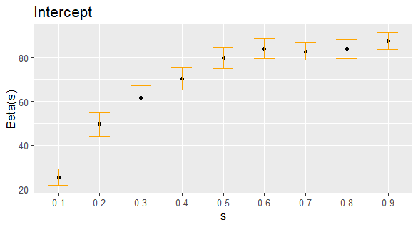
Appendix B Supplementary simulation results

This section provides the detailed simulation results under incompletely observed outcome functions. As described in the main text, we suppose that for each unit i𝑖i we can observe {(si,j,qi(yi,j))}j=1msuperscriptsubscriptsubscript𝑠𝑖𝑗subscript𝑞𝑖subscript𝑦𝑖𝑗𝑗1𝑚\{(s_{i,j},q_{i}(y_{i,j}))\}_{j=1}^{m}, where si,jsubscript𝑠𝑖𝑗s_{i,j}’s are uniformly randomly drawn from [0,1]01[0,1], for m{15,50}𝑚1550m\in\{15,50\}. To recover the entire functional form of the qisubscript𝑞𝑖q_{i} function, we apply the linear interpolation method in (3.3). The simulation scenarios examined are all identical to those used in the main text. The results for the 2SLS estimator and the Wald test are summarized in Tables B1 and B2, respectively.

Table B1: Estimation performance
β𝛽\beta α𝛼\alpha (λc=0.5subscript𝜆𝑐0.5\lambda_{c}=0.5) α𝛼\alpha (λc=1subscript𝜆𝑐1\lambda_{c}=1) α𝛼\alpha (λc=2subscript𝜆𝑐2\lambda_{c}=2) α𝛼\alpha (λc=3subscript𝜆𝑐3\lambda_{c}=3)
DGP m𝑚m n𝑛n # knots BIAS RMSE BIAS RMSE BIAS RMSE BIAS RMSE BIAS RMSE
1 15 400 2 0.0002 0.0376 0.0214 0.1071 0.0228 0.1036 0.0203 0.1022 0.0162 0.1010
3 0.0004 0.0385 0.0221 0.1199 0.0230 0.1157 0.0197 0.1136 0.0149 0.1119
1600 2 0.0008 0.0184 0.0161 0.0974 0.0201 0.0962 0.0223 0.0978 0.0220 0.0991
3 0.0007 0.0184 0.0170 0.1118 0.0208 0.1097 0.0226 0.1105 0.0220 0.1112
50 400 2 -0.0010 0.0370 0.0202 0.1060 0.0214 0.1025 0.0189 0.1010 0.0148 0.0997
3 -0.0008 0.0372 0.0208 0.1187 0.0217 0.1147 0.0184 0.1125 0.0136 0.1108
1600 2 -0.0004 0.0176 0.0152 0.0959 0.0190 0.0951 0.0211 0.0968 0.0208 0.0980
3 -0.0004 0.0177 0.0161 0.1102 0.0197 0.1086 0.0214 0.1094 0.0208 0.1102
2 15 400 2 -0.0001 0.0377 -0.0023 0.0917 -0.0065 0.0829 -0.0134 0.0769 -0.0196 0.0742
3 0.0002 0.0388 -0.0023 0.1074 -0.0067 0.0990 -0.0143 0.0931 -0.0211 0.0903
1600 2 0.0007 0.0184 -0.0001 0.0848 -0.0024 0.0808 -0.0060 0.0774 -0.0091 0.0757
3 0.0007 0.0184 0.0001 0.1015 -0.0023 0.0976 -0.0061 0.0942 -0.0094 0.0925
50 400 2 -0.0012 0.0375 -0.0011 0.0921 -0.0055 0.0836 -0.0125 0.0775 -0.0188 0.0748
3 -0.0012 0.0376 -0.0011 0.1078 -0.0058 0.0996 -0.0134 0.0937 -0.0203 0.0908
1600 2 -0.0005 0.0179 0.0013 0.0851 -0.0012 0.0813 -0.0049 0.0780 -0.0081 0.0763
3 -0.0005 0.0181 0.0014 0.1018 -0.0011 0.0981 -0.0051 0.0948 -0.0085 0.0930
3 15 400 2 -0.0004 0.0401 0.0074 0.1841 0.0100 0.1964 0.0076 0.2076 0.0027 0.2125
3 -0.0004 0.0410 0.0079 0.1870 0.0099 0.2008 0.0065 0.2125 0.0008 0.2172
1600 2 0.0007 0.0195 0.0006 0.1559 0.0061 0.1708 0.0096 0.1885 0.0098 0.1977
3 0.0007 0.0197 0.0016 0.1552 0.0067 0.1732 0.0098 0.1927 0.0094 0.2024
50 400 2 -0.0014 0.0395 0.0142 0.1823 0.0171 0.1946 0.0148 0.2061 0.0100 0.2112
3 -0.0014 0.0399 0.0148 0.1852 0.0170 0.1993 0.0138 0.2116 0.0081 0.2165
1600 2 -0.0005 0.0192 0.0071 0.1545 0.0127 0.1682 0.0165 0.1862 0.0168 0.1957
3 -0.0005 0.0192 0.0081 0.1533 0.0134 0.1707 0.0167 0.1907 0.0165 0.2009
Table B2: Rejection frequency
ϱ=0italic-ϱ0\varrho=0 ϱ=0.1italic-ϱ0.1\varrho=0.1 ϱ=0.2italic-ϱ0.2\varrho=0.2
n𝑛n # knots m𝑚m λcsubscript𝜆𝑐\lambda_{c} 10% 5% 1% 10% 5% 1% 10% 5% 1%
400 2 15 0.5 0.071 0.035 0.016 0.261 0.194 0.105 0.967 0.939 0.829
1 0.063 0.035 0.020 0.710 0.608 0.440 1.000 0.998 0.992
2 0.056 0.032 0.015 0.946 0.921 0.861 1.000 1.000 1.000
3 0.051 0.035 0.019 0.974 0.959 0.921 1.000 1.000 1.000
50 0.5 0.079 0.049 0.018 0.298 0.210 0.110 0.983 0.967 0.880
1 0.077 0.048 0.019 0.737 0.641 0.469 1.000 0.998 0.995
2 0.069 0.040 0.019 0.969 0.945 0.903 1.000 1.000 1.000
3 0.062 0.044 0.023 0.981 0.975 0.955 1.000 1.000 1.000
3 15 0.5 0.068 0.034 0.016 0.242 0.178 0.096 0.955 0.919 0.797
1 0.060 0.034 0.016 0.690 0.590 0.430 1.000 0.998 0.991
2 0.052 0.031 0.013 0.941 0.912 0.844 1.000 1.000 1.000
3 0.045 0.033 0.016 0.964 0.950 0.917 1.000 1.000 1.000
50 0.5 0.073 0.046 0.018 0.292 0.205 0.105 0.980 0.959 0.872
1 0.072 0.044 0.018 0.741 0.650 0.479 1.000 0.999 0.995
2 0.061 0.036 0.017 0.965 0.941 0.901 1.000 1.000 1.000
3 0.061 0.041 0.023 0.979 0.970 0.955 1.000 1.000 1.000
1600 2 15 0.5 0.058 0.043 0.023 0.505 0.364 0.188 0.998 0.996 0.991
1 0.057 0.043 0.023 0.936 0.875 0.692 1.000 1.000 0.999
2 0.063 0.040 0.022 0.997 0.997 0.990 1.000 1.000 1.000
3 0.064 0.041 0.022 0.999 0.999 0.998 1.000 1.000 1.000
50 0.5 0.078 0.054 0.028 0.611 0.449 0.243 1.000 1.000 1.000
1 0.078 0.053 0.029 0.970 0.942 0.791 1.000 1.000 1.000
2 0.077 0.052 0.028 1.000 1.000 0.998 1.000 1.000 1.000
3 0.078 0.052 0.026 1.000 1.000 1.000 1.000 1.000 1.000
3 15 0.5 0.056 0.041 0.023 0.501 0.353 0.176 0.999 0.996 0.990
1 0.055 0.041 0.022 0.940 0.869 0.695 1.000 1.000 0.999
2 0.062 0.039 0.021 0.998 0.997 0.990 1.000 1.000 1.000
3 0.061 0.040 0.020 1.000 0.999 0.998 1.000 1.000 1.000
50 0.5 0.074 0.051 0.027 0.605 0.439 0.236 1.000 1.000 1.000
1 0.074 0.050 0.028 0.972 0.942 0.808 1.000 1.000 1.000
2 0.076 0.050 0.028 1.000 1.000 0.999 1.000 1.000 1.000
3 0.077 0.049 0.026 1.000 1.000 1.000 1.000 1.000 1.000

Appendix C Supplementary material for the empirical analysis in Section 5

Table C3: Descriptive statistics (n=1883𝑛1883n=1883)
Variable Mean Std. Dev. Min. Max.
Landprice 10.083 1.191 7.313 14.883
Unemployment 3.687 1.134 0 10.635
Agriculture 0.078 0.081 0 0.467
Sales 10.500 2.196 0 17.666
Beds 1.089 1.051 0 13.489
Childcare 0.290 0.209 0.000 2.833
q(0.25)𝑞0.25q(0.25) 31.801 5.638 17.904 58.162
q(0.5)𝑞0.5q(0.5) 52.777 5.865 38.113 71.003
q(0.75)𝑞0.75q(0.75) 69.895 3.877 54.193 99.028

Definitions: Landprice = log(average residential landprice (JPY/m2)); Unemployment = unemployment rate (%); Agriculture = proportion of agriculture, forestry, and fishery workers; Sales = log(annual commercial sales (million JPY) + 1); Beds = 100 ×\times # of hospital beds/population; Childcare = 1000 ×\times # of childcare facilities/population.

Refer to caption
Refer to caption
Refer to caption
Refer to caption
Refer to caption
Refer to caption
Refer to caption
Figure C1: Estimated coefficients