Generalizing Reward Modeling
for Out-of-Distribution Preference Learning

Abstract

Preference learning (PL) with large language models (LLMs) aims to align the LLMs’ generations with human preferences. Previous work on reinforcement learning from human feedback (RLHF) has demonstrated promising results in in-distribution PL. However, due to the difficulty of obtaining human feedback, discretely training reward models for every encountered distribution is challenging. Thus, out-of-distribution (OOD) PL is practically useful for enhancing the generalization ability of LLMs with limited preference feedback. This work addresses OOD PL by optimizing a general reward model through a meta-learning approach. During meta-training, a bilevel optimization algorithm is utilized to learn a reward model capable of guiding policy learning to align with human preferences across various distributions. When encountering a test distribution, the meta-test procedure conducts regularized policy optimization using the learned reward model for PL. We theoretically demonstrate the convergence rate of the bilevel optimization algorithm under reasonable assumptions. Additionally, we conduct experiments on two text generation tasks across 20 held-out domains and outperform a variety of strong baselines across various evaluation metrics.

1 Introduction

Aligning large language models (LLMs) with human preferences through reinforcement learning (RLHF) has been demonstrated as a practical approach to align pretrained LLMs along human values. As demonstrated by recent research on LLMs (Christiano et al., 2017; Ziegler et al., 2019; Stiennon et al., 2020; Ouyang et al., 2022), RLHF initially trains a reward model to capture human preferences from a dataset of pairwise comparisons. It then aligns the LLMs with the learned reward model through regularized policy optimization, aiming to learn a language policy that better reflects human values. However, defining precise rewards for various real-world tasks is non-trivial (McKinney et al., 2022), and obtaining high-quality feedback that accurately represents human preferences is challenging Bai et al. (2022).

Most previous work on RLHF focuses on in-distribution preference learning (Casper et al., 2023). For example, when conducting sentiment generation for the film distribution, RLHF utilizes only the in-distribution preference data for reward learning and performs regularized policy optimization with the in-distribution data. However, two major challenges arise when encountering the distribution shift problem. For example, Figure 1 illustrates a scenario where preference data from the book and dvd domains are used for reward modeling, and regularized policy optimization is conducted with data from the book distribution. The first challenge is that the generations from the policy may substantially deviate from the human preferences of the target distribution, posing an out-of-distribution (OOD) challenge for preference learning. Furthermore, these distribution shifts result in policy drift during the policy optimization process with Kullback-Leibler divergence (Ramamurthy et al., 2023; Rafailov et al., 2024): the policy tends to move towards the reference policy largely followed in the training distribution, exacerbating the model’s deviation from the target distribution in preference learning.

An initial approach to addressing the out-of-distribution (OOD) challenge is to directly enhance the OOD generalization ability of the reward model using preference data from multiple distributions. This specific approach may involve employing multi-task learning to train a reward model using data from various distributions or integrating reward models from multiple domains into a unified model, similar to previous work on reward model ensembling (Ramé et al., 2024). However, solely improving reward modeling for OOD reward prediction within the scope of preference learning may be suboptimal, considering that the objective of preference learning is to optimize a policy aligned with human preferences. To better tackle the OOD challenge, we employ an end-to-end strategy to learn a reward function capable of guiding policy optimization for OOD preference learning. To achieve this, we utilize a meta-learning approach to directly compute OOD preferences based on the predicted probabilities generated by a language policy. This policy is optimized w.r.t. a reward-model-based objective for policy optimization using in-distribution fine-tuning data. In particular, we incorporate a regularization term in policy optimization to penalize the Kullback-Leibler divergence between the predicted distribution by the policy and the sampling distribution of examples from the target distribution, thereby mitigating the challenge of policy drift.

To implement the above approach, we propose a gradient-based bilevel optimization algorithm. Specifically, the outer loop performs a sufficient number of stochastic gradient descent (SGD) iterations to achieve convergence and optimize the out-of-distribution (OOD) preference learning objective with respect to the reward model. The inner loop performs SGD updates for the in-distribution policy using the reward model. As illustrated in Figure 1, the entire training process comprises a meta-training phase and a meta-test phase. In the meta-test phase, a sufficient number of SGD iterations are conducted to optimize a language policy with the meta-learned reward model using supervised samples from the test distribution. Theoretically, we establish an upper bound for the convergence rate of bilevel optimization with respect to the learning rates of inner-loop and outer-loop optimization, as well as the controlling factor for reward modeling. Empirically, we conduct experiments on both controlled sentiment generation and knowledge answer generation, using multiple metrics for evaluation. The results demonstrate that our method outperforms a range of strong baselines for OOD preference learning and achieves the best results across four domains of sentiment generation and 18 domains of answer generation.

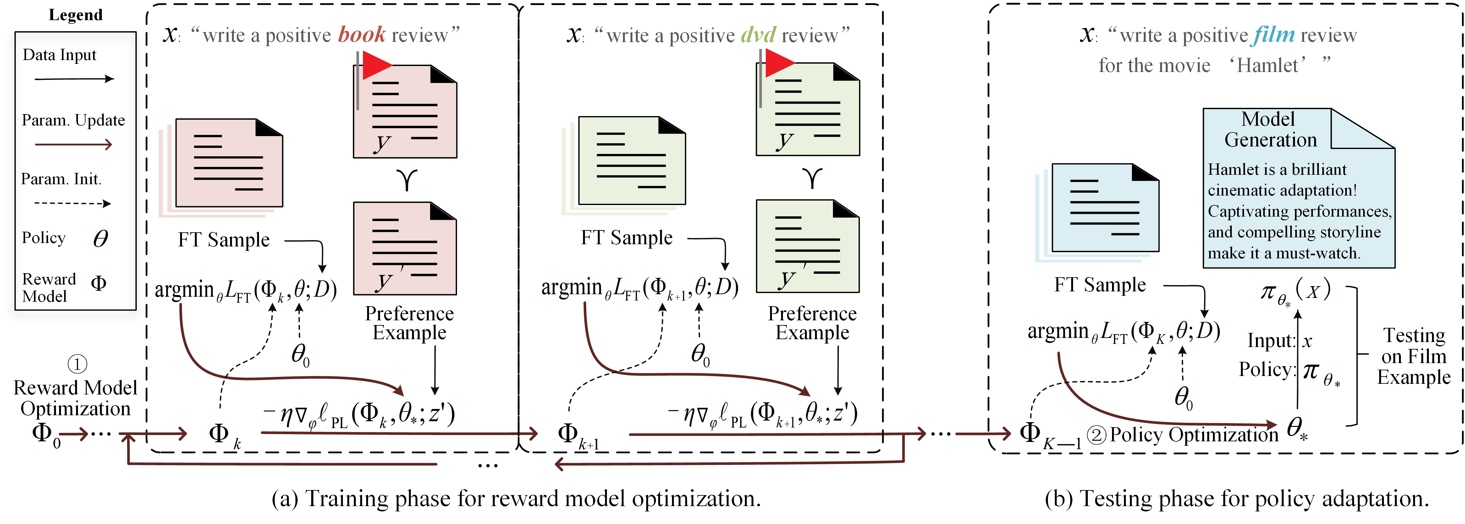
Figure 1: The meta-learning phase and testing phase are crucial for out-of-distribution preference learning. During the meta-training phase, the reward model $\Phi$ is optimized using $K$ iterations of stochastic gradient descent (SGD) on preference examples and fine-tuning samples from training distributions, such as the book and dvd distributions. Upon encountering an unseen distribution film during the testing phase, the optimized reward model $\Phi_{K}$ from the meta-training phase is utilized, and only the in-distribution fine-tuning samples are used to optimize the in-distribution policy $\theta_{*}$.

2 Preliminaries

Problem Setting	Training		Inference
	preference data	fine-tuning data
SFT	-	$\mathcal{D}^{tr}$, $\mathcal{D}^{te}$	$\mathcal{D}^{te}$
in-distribution PL	$\mathcal{D}_{\rm PL}^{tr}$, $\mathcal{D}^{te}_{\rm PL}$	$\mathcal{D}^{tr}$, $\mathcal{D}^{te}$	$\mathcal{D}^{te}$
out-of-distribution PL	$\mathcal{D}_{\rm PL}^{tr}$	$\mathcal{D}^{tr}$, $\mathcal{D}^{te}$	$\mathcal{D}^{te}$

Table 1: Problem Setting. $\mathcal{D}{\rm PL}^{tr}$ and $\mathcal{D}{\rm PL}^{te}$ represent preference data from the training and testing distributions, respectively, while $\mathcal{D}^{tr}$ and $\mathcal{D}^{te}$ denote fine-tuning data from the training and testing distributions, respectively.

Notations.

Building on the work of Azar et al. (2023); Rafailov et al. (2024), we define the preference learning objective as learning a language model policy $\pi_{\theta}$ parameterized by $\theta$. Specifically, given a language prompt $x$ drawn from the input distribution $\mathcal{D}_{X}$ over the input space $\mathcal{X}$, the policy computes the probability distribution $\pi(\cdot|x)$ over the answer space $\mathcal{Y}_{x}$ and the predicted answer is denoted as $\hat{y}=\mathop{\arg\max}_{y\in\mathcal{Y}_{x}}\pi_{\theta}(y|x)$. Traditional supervised fine-tuning uses prompt-response pairs $(x,y)$ drawn from a joint distribution $\mathcal{D}_{XY}$ for alignment learning. In this paper, we use $\mathcal{D}$ to represent both $\mathcal{D}_{X}$ and $\mathcal{D}_{XY}$ for brevity. To align with the human preferences for answer generation using pretrained language models, preference learning utilizes pairs of answers corresponding to a prompt, $\{y,y^{\prime},x:y\succ y^{\prime}|x\}$, drawn from a distribution $\mathcal{D}_{\rm PL}$ where $y\succ y^{\prime}|x$ indicates that $y$ is the preferred answer over dispreferred answer $y^{\prime}$ given the prompt $x$.

Supervised fine-tuning (SFT).

SFT involves fine-tuning a pretrained LLM to adapt to task-specific datasets. The SFT process involves employing a supervised learning objective, specifically maximum likelihood estimation (MLE), on a carefully curated high-quality dataset, denoted as $\mathcal{D}$. The training objective is to obtain a language policy $\pi_{\theta}$ that satisfies

$$\min_{\theta}-\mathbb{E}_{(x,y)\sim\mathcal{D}}\left[\log\pi_{\theta}(y|x)\right]$$ (1)

RLHF with reward modeling.

The standard RLHF framework (Ziegler et al., 2019; Ouyang et al., 2022) for aligning human preferences with language models comprises two main phases: (i) learning a reward model for a specific task, and (ii) fine-tuning the policy with the learned reward model. During the reward model learning phase, given a pairwise data distribution $\mathcal{D}_{\rm PL}$, a reward model $r_{\phi}:(x,y)\mapsto r_{\phi}(x,y)\in\mathbb{R}$ parameterized by $\phi$ is trained to score preference of $y$ to be the answer of $x$, using a maximum likelihood estimation (MLE) loss function:

$$\mathcal{L}_{R}=-\mathbb{E}_{(x,y\succ y^{\prime})\sim\mathcal{D}_{\rm PL}}\left[\log\sigma\left(r_{\phi}(x,y)-r_{\phi}(x,y^{\prime})\right)\right],$$ (2)

where $\sigma$ denotes the logistic function. In the RL fine-tuning phase, given a prompt distribution $\mathcal{D}$, the optimization objective can be represented as follows,

$$\max_{{\theta}}\mathbb{E}_{x\sim\mathcal{D}}\left[\mathbb{E}_{y\sim\pi_{\theta}(\cdot|x)}\left[r_{\phi}(x,y)\right]-\beta\mathrm{D}_{\rm KL}\left(\pi_{\theta}(\cdot|x)||\pi_{\rm ref}(\cdot|x)\right)\right],$$ (3)

where $\mathrm{D}{\rm KL}(\cdot||\cdot)$ represents the Kullback-Leibler divergence, $\pi{\rm ref}(\cdot|x)$ denotes a reference distribution, and $\beta$ is the balancing coefficient. Previous work, such as RLHF-PPO(Ramamurthy et al., 2023) and DPO Rafailov et al. (2024), uses an SFT model as the $\pi_{\rm ref}$ to impose constraints on the similarity between the predictions of the RLHF model and those of the initial SFT model. In this study, we revise the constraint using $\pi_{\rm ref}$ to accommodate meta-learning for generalization across domains, as detailed in §3.

Problem Setting.

We compare three problem settings for language policy learning, as shown in Table 1. To ensure a fair comparison, we consider a transfer learning scenario where all learning settings utilize supervised fine-tuning data from both the training and test distributions $\mathcal{D}^{tr}$, $\mathcal{D}^{te}$ during training, and employ prompting from the test distribution $\mathcal{D}^{te}$ during inference. In contrast to supervised fine-tuning (SFT), preference learning (PL) utilizes additional human preference data for training, as demonstrated in previous works (Christiano et al., 2017; Ouyang et al., 2022; Zhang et al., 2023; Liu et al., 2023; Rafailov et al., 2024). In the in-distribution PL setting, similar to previous approaches such as RLHF-PPO (Christiano et al., 2017) and DPO Rafailov et al. (2024), preference data from both the training and test distributions are used for training. This work focuses on an out-of-distribution PL setting where only preference data from the training distribution are used for training, and fine-tuning data from both the training and testing distributions are used for policy optimization.

3 Meta-Learning for Generalizing Reward Modeling

Bilevel Programming	Reward Optimization (in-distribution)	Meta-Learning (out-of-distribution)
outer variables	reward model $\phi$	generalized reward model $\phi$
outer objective	PL objective $\mathcal{L}_{\rm PL}(\phi,\theta_{*},\mathcal{D}_{\rm PL})$ (Eq. (7))	PL objective ${\bf L}(\phi)$ (Eq. (11))
inner variables	policy $\theta$	policies of each distribution $\{\theta^{T}\}_{T\in\mathcal{D}_{\mathcal{T}}}$
inner objective	FT objective $\mathcal{L}_{\rm FT}(\phi,\theta,\mathcal{D})$ (Eq. (10))	FT objectives for each distribution $\{\mathcal{L}_{\rm FT}(\phi,\theta,\mathcal{D}^{T})\}_{T\in\mathcal{D}_{\mathcal{T}}}$ (Eq. (12))

Table 2: Linkes and naming conventions among different fields of bilevel optimization in this work.

To develop a meta-learning approach for generalizing reward modeling, we employ bilevel programming, building on previous research on meta-learning for generalization (Finn et al., 2017; Franceschi et al., 2018; Li et al., 2018; Ji et al., 2021). In this section, we first introduce a bilevel optimization framework for optimizing rewards in §3.1. Following the bilevel optimization framework, we then introduce the meta-learning approach for OOD PL in §3.2. Table 2 outlines the connections among bilevel programming, in-distribution reward optimization, and meta-learning for OOD PL. Additionally, we introduce a gradient-based algorithm for optimizing the meta-learning objective in §3.3 and analyze the theoretical convergence rate in §3.4.

3.1 Reward Optimization via Bilevel Programming

Bilevel programming.

In this section, we consider a bilevel optimization problem (see e.g., (Colson et al., 2007; Sinha et al., 2017)) of the form:

$$\min_{\phi}\mathcal{L}_{\rm PL}({\phi},{\theta_{*}};\mathcal{D}_{\rm PL});$$ (4)

$${\rm s.t.}\ \theta_{*}\in\mathop{\arg\min}_{\theta}\mathcal{L}_{\rm FT}({\phi},{\theta};\mathcal{D}),$$ (5)

where $\mathcal{L}_{\rm PL}$ represents the outer objective, and for every reward function $r_{\phi}$, $\mathcal{L}_{\rm FT}$ represents the inner objective. Note that $\theta_{*}$ denotes the optimal parameters of a policy w.r.t. a reward model $r_{\phi}$ by RLHF fine-tuning via minimizing the inner objective $\mathcal{L}_{\rm FT}$.

Outer objective.

In the context of reward optimization, we desire that the fine-tuned policy ${\theta}_{*}$, with the help of the reward function $r_{\phi}$, can align with human preferences. In particular, given a pair of answers for a prompt $x$ with preference ranking, $(y,y^{\prime},x:y\succ y^{\prime}|x)\sim\mathcal{D}_{\rm PL}$, we use the Bradley-Terry (BT) model (Bradley & Terry, 1952) to compute the comparing preference of $p(y\succ y^{\prime}|x)$ w.r.t. a fine-tuned policy ${\theta_{*}}$ as follows

$$p_{*}(y\succ y^{\prime}|x)=\frac{\pi_{\theta_{*}}(y|x)}{\pi_{\theta_{*}}(y|x)+\pi_{\theta_{*}}(y^{\prime}|x)}$$ (6)

Given a preference sampling distribution (a.k.a. a dataset) $\mathcal{D}_{\rm PL}=\{z=(x,y,y^{\prime})\}$, we apply the maximum likelihood estimation (MLE) to define the outer objective of preference alignment w.r.t. the policy ${\theta_{*}}$ as follows

$$\begin{split}&\min_{\phi}\mathcal{L}_{\rm PL}(\phi,\theta_{*};\mathcal{D}_{\rm PL})=\min_{{\phi}}\mathbb{E}_{z\sim\mathcal{D}_{\rm PL}}\left[\ell_{\rm PL}({\phi},{\theta}_{*},z)\right]\\ &{\rm s.t.}\ \ell_{\rm PL}\left({\phi},{\theta}_{*},z\right)=-\log\sigma\left(\log\pi_{\theta_{*}}(y|x)-\log\pi_{\theta_{*}}(y^{\prime}|x)\right)\end{split}$$ (7)

Inner objective.

For the inner-loop optimization, we consider the objective of RLHF fine-tuning in Eq. (3), and specify the reference policy as the sampling distribution for the target task to avoid the policy drift problem that the learned policy may move towards the source distribution. In particular, given a target distribution $\mathcal{D}$, the reference distribution is represented as the sampling distribution of $\mathcal{D}$, i.e., $\pi_{\rm ref}(\cdot|x):=\hat{\mu}(\cdot|x)$ for any $x\sim\mathcal{D}$. Then, the RLHF fine-tuning objective can be represented as

$$\mathop{\arg\max}_{{\theta}}\mathbb{E}_{x\sim\mathcal{D}}\left[\mathbb{E}_{y\sim\pi_{\theta}(\cdot|x)}\left[r_{\phi}(x,y)\right]-\beta\mathrm{D}_{\rm KL}\left(\pi_{\theta}(\cdot|x)||\hat{\mu}(\cdot|x)\right)\right]$$ (8)

However, it is unsolvable to directly optimize the above objective using the policy gradient optimization approach Schulman et al. (2015; 2017), since the sampling distribution is unknown. Thus, we consider an approximate solution to this optimization objective. This derivation largely follows Peters & Schaal (2007); Peng et al. (2019). The major observation is that the objective is strictly concave and thus we can use the Karush-Kuhn-Tucker conditions (Boyd & Vandenberghe, 2004) to obtain a globally optimal solution to Eq. (8) such that for any $x\sim\mathcal{D}$ and $y\in\mathcal{Y}_{x}$,

$$\pi_{*}(y|x)=\frac{1}{Z(x)}\hat{\mu}(y|x)\exp\left(\frac{1}{\beta}r_{\phi}(x,y)\right),$$ (9)

where $Z(x)$ represents the partition function. A detailed derivation is available in Appendix A. We focus on a parameterized estimator (e.g., a neural network) to tackle a parameter estimation problem $\min_{{\theta}}\mathbb{E}_{x\sim\mathcal{D}}[\mathrm{D}_{\rm KL}(\pi_{*}(\cdot|x)||\pi_{\theta}(\cdot|x))]$. Thereby, given a fine-tuning sampling distribution $\mathcal{D}=\{z=(x,y)\}$, the inner objective can be represented as a logical regression formulaion,

$$\begin{split}&\mathop{\arg\min}_{\theta}\mathcal{L}_{\rm FT}(\phi,\theta,\mathcal{D})=\mathop{\arg\min}_{\theta}\mathbb{E}_{x\sim\mathcal{D}}\mathbb{E}_{y\sim\hat{\mu}(y|x)}\left[\ell_{\rm FT}({\phi},{\theta},z)\right]\\ &\qquad\qquad\qquad\qquad\quad=\mathop{\arg\min}_{\theta}\mathbb{E}_{z\sim\mathcal{D}}\left[\ell_{\rm FT}({\phi},{\theta},z)\right]\\ &{\rm s.t.}\ \ell_{\rm FT}({\phi},{\theta},z)=-\log\pi_{\theta}(y|x)\exp\left(\frac{1}{\beta}r_{\phi}(x,y)\right)\end{split}$$ (10)

3.2 Meta-Learning

In this section, we generalize the in-distribution bilevel optimization framework to tackle the out-of-distribution (OOD) preference learning. To this end, we assume that there exists a meta-distribution $\mathcal{D}_{\mathcal{T}}$ over the set of distributions $\mathcal{T}$, e.g., $\mathcal{T}:=\{{\tt book},{\tt dvd},{\tt film},\ldots\}$. Previous study on the distribution-level generalization refers to meta-learning (Baxter, 2000; Vilalta & Drissi, 2002; Finn et al., 2017).

In order to learn a generalized reward modeling for fine-tuning unseen distribution in the test phase, we utilize a meta-learning framework for reward optimization. To this end, the outer objective described in the Section 3.1 should be extent to computing the preference loss over multiple distributions, while the inner objective can be unchangeable as a fine-tuning objective for each training distribution. In particular, given a distribution $T\in\mathcal{T}$, there exists a distribution-specific fine-tuning sampling distribution $\mathcal{D}^{T}$. For preference learning, each training distribution has a preference sampling distribution $z=(x,y,y^{\prime})\sim\mathcal{D}^{T}_{\rm PL}$. The optimal variable in inner objective should be the distribution-specific policy ${\theta^{T}_{*}}$. A key point is that the reward model ${\phi}$ is shared across all distributons. With this notation the inner and outer objectives can be represented as follows.

$$\min_{\phi}{\bf L}(\phi)=\min_{\phi}\mathbb{E}_{T\sim\mathcal{D}_{\mathcal{T}}}\mathbb{E}_{z\sim\mathcal{D}^{T}_{\rm PL}}\left[\ell_{\rm PL}\left(\phi,\theta^{T}_{*},z\right)\right]$$ (11)

$${\rm s.t.}\ \theta^{T}_{*}\in\mathop{\arg\min}_{{\theta^{T}}}\mathbb{E}_{z\sim\mathcal{D}^{T}}\left[\ell_{\rm PL}({\phi},{\theta^{T}},z)\right],$$ (12)

where the objective function $\ell_{\rm PL}(\phi,{\theta^{T}_{*}},z)$, $z\sim\mathcal{D}^{T}_{\rm PL}$ represents the preference learning loss, which has a same formulation as the in-distribution version of Eq. (7), and $\ell_{\rm FT}(\phi,\theta^{T},z)$, $z\sim\mathcal{D}^{T}$ represents the fine-tuning loss, which has the same formulation as the in-distribution version of Eq. (10).

3.3 Gradient-Based Algorithm

Input: Meta-training data $\{\mathcal{D}^{T}_{\rm PL},\mathcal{D}^{T}\}_{T\in\mathcal{T}_{tr}}$, reward model $\phi$, policy $\theta$

Output: Optimal reward model $\phi_{*}$ for meta-test in Algorithm 2

for $k=0,1,2,\ldots,K$ do

       Randomly draw a sample distribution $T\in\mathcal{T}_{tr}$ from the meta-distribution $\mathcal{D}_{\mathcal{T}}$

       Parameter initialization $\theta\leftarrow\theta_{0}$

       for $t=0,1,2,\ldots,D$ do

             Randomly draw a sample $z_{k,t}$ from $\mathcal{D}^{T}$

             Update $\theta_{k,t+1}\leftarrow\theta_{k,t}-\alpha\nabla_{\theta}\ell_{\rm FT}(\phi_{k},\theta_{k,t};z_{k,t})$$\hfill\rhd$ minimize the inner objective of Eq. (12)

            

       end for

      Randomly draw a sample $z_{k}$ from $\mathcal{D}^{T}_{\rm PL}$

       Update $\phi_{k+1}\leftarrow\phi_{k}-\eta\nabla_{\phi}\ell_{\rm PL}(\phi_{k},\theta_{k,D};z_{k})$ $\hfill\rhd$ minimize the outer objective of Eq. (11)

end for

Algorithm 1 Meta-training procedure

Input: Meta-test data $\mathcal{D}^{te}$; optimized reward function $\phi_{*}$ from Algorithm 1

Output: Optimal policy $\theta_{*}$ for testing

Parameter initialize $\theta\leftarrow\theta_{0}$

while not converge or not reach stopping conditions do

       Randomly draw a sample $z$ from $\mathcal{D}^{te}$

       Update $\theta\leftarrow\theta-\alpha\nabla_{\theta}\ell_{\rm FT}(\phi_{*},\theta;z)$ $\hfill\rhd$ minimize the inner objective of Eq. (12)

end while

Algorithm 2 Meta-test procedure

Following the previous work on gradient-based bilevel programming (Finn et al., 2017; Franceschi et al., 2018; Ji et al., 2021), we use a gradient-based approach to tackle the bilevel optimization objective in Eq. (11) and Eq. (12). The whole training process consists of a meta-training procedure and a meta-test procedure.

Meta-training.

As shown in Algorithm 1, for each iteration $k\in{1,\ldots,K}$ in the outer-loop optimization, the inner-loop process runs $D$ steps of stochastic gradient decent (SGD) to gain an optimal solution of ${\theta}_{*}$ with $\theta_{k,D}$. Then, the outer-loop process uses SGD optimization w.r.t. $\phi_{k}$ via computes the gradient $\mathbb{E}\left[\frac{\partial\ell_{\rm PL}(\phi_{k},\theta_{k,D})}{\partial\phi_{k}}\right]$ as an approximation of the hyper-gradient $\mathbb{E}\left[\frac{\partial\ell_{\rm PL}(\phi_{k},{\theta}_{*})}{\partial\phi_{k}}\right]$. Specifically, we compute the explicit form of the $\frac{\partial\ell_{\rm PL}(\phi_{k},\theta_{k,D})}{\partial\phi_{k}}$ in the following proposition.

Proposition 1.

For any outer-loop step $k\in\{0,1,2,\ldots,K-1\}$, with the outer-loop input $z_{k}$ and the inner-loop inputs $\{z_{k,t}\}_{t=0}^{D-1}$, the gradient w.r.t. $\phi_{k}$ $\frac{\partial\ell_{\rm PL}(\phi_{k},\theta_{k,D})}{\partial\phi_{k}}$ takes the analytical form,

$$\begin{split}\frac{\partial\ell_{\rm PL}(\phi_{k},\theta_{k,D})}{\partial{\phi}_{k}}=&\frac{\alpha}{\beta}\left(\nabla_{\theta}\log\pi_{\theta_{k,D}}(y_{k}|x_{k})-\nabla_{\theta}\log\pi_{\theta_{k,D}}(y^{\prime}_{k}|x_{k})\right)\\ &\cdot\sum_{t=0}^{D-1}\bigg{\{}\exp\left(\frac{1}{\beta}r_{\phi_{k}}(x_{k,t},y_{k,t})\right)\nabla_{\theta}\log\pi_{\theta_{k,t}}(y_{k,t}|x_{k,t})\\ &\cdot\prod_{j=t+1}^{D-1}\left(I+\alpha\exp\left(\frac{1}{\beta}r_{\phi_{k}}(x_{k,t},y_{k,t})\right)\nabla_{\theta}^{2}\log\pi_{\theta_{k,t}}(y_{k,t}|x_{k,t})\right)\bigg{\}}\end{split}$$ (13)

Proof.

The major proof steps consists of the chain rule of partial differentiation, and the detailed derivation is available in Appendix B. ∎

Finally, the meta-training procedure outputs an optimized reward function parameterized by $\phi_{*}$.

Meta-test.

As shown in Algorithm 2, the meta-test procedure takes the optimal reward model $\phi_{*}$ from meta-training to learn a policy for a given test distribution. In particular, the meta-test process computes policy gradients based on the optimal reward model $\phi_{*}$ and uses SGD to optimize the distribution-specific policy with a sufficient number of iterations for convergence. The meta-test procedure can also be viewed as test-phase adaptation.

3.4 Convergence Analysis

Following previous work on convergence analysis of SGD (Drori & Shamir, 2020; Ji et al., 2021), we study the convergence rate of the proposed SGD-based bilevel programming to the stationary point. In particular, we aim to show how the proposed algorithm minimizes $\mathbb{E}[\|\nabla_{\phi}{\bf L}(\overline{\phi})\|^{2}]$, where ${\bf L}(\phi)$ is defined in Eq. (11) and $\overline{\phi}$ denotes the output of the algorithm.

Following previous work on the convergence rate of gradient-based bilevel optimization (Ji et al., 2021), we focus on the following types of basic loss functions w.r.t. the policy for preference learning.

Assumption 1.

The maximum likelihood estimation (MLE) objective for policy learning, $-\log\pi_{\theta}$, is $\mu$-strongly convex.

Besides, we take the following standard Lipschitz assumptions on the basic MLE loss functions of policy $-\log\pi_{\theta}$ and the reward function $r_{\phi}$, which are largely followed those have been widely adopted in bilevel optimization (Ghadimi & Wang, 2018; Ji et al., 2021).

Assumption 2.

The loss function $-\log\pi_{\theta}$ and reward function $r_{\phi}$ satisfy

• $-\log\pi_{\theta}(y|x)$ is $M$-Lipschitz, i.e., for any $\theta,\theta^{\prime}$ and any $(x,y)$,

  $$\left|\log\pi_{\theta}(y|x)-\log\pi_{\theta^{\prime}}(y|x)\right|\leq M\|\theta-\theta^{\prime}\|$$ (14)

• $-\nabla\log\pi_{\theta}(y|x)$ is $L$-Lipschitz, i.e., for any $\theta,\theta^{\prime}$ and any $(x,y)$,

  $$\|\nabla\log\pi_{\theta}(y|x)-\nabla\log\pi_{\theta^{\prime}}(y|x)\|\leq L\|\theta-\theta^{\prime}\|$$ (15)

• $-\nabla^{2}\log\pi_{\theta}(y|x)$ is $\rho$-Lipschitz, i.e., for any $\theta,\theta^{\prime}$ and any $(x,y)$,

  $$\|\nabla^{2}\log\pi_{\theta}(y|x)-\nabla^{2}\log\pi_{\theta^{\prime}}(y|x)\|\leq\rho\|\theta-\theta^{\prime}\|$$ (16)

• $r_{\phi}$ is $T$-Lipschitz, i.e., for any $\phi,\phi^{\prime}$ and any $(x,y)$,

  $$\left|r_{\phi}(x,y)-r_{\phi^{\prime}}(x,y)\right|\leq T\|\phi-\phi^{\prime}\|$$ (17)

• $\nabla r_{\phi}(x,y)$ is $P$-Lipschitz, i.e., for any $\phi,\phi^{\prime}$ and any $(x,y)$,

  $$\left\|\nabla r_{\phi}(x,y)-\nabla r_{\phi^{\prime}}(x,y)\right\|\leq P\|\phi-\phi^{\prime}\|$$ (18)

Besides, we also consider the following reasonable assumptions on the boundnesses of reward function and predicted probability by the policy.

Assumption 3.

The function $-\log\pi_{\theta}(y|x)$ and $\exp(r_{\phi}(x,y))$ are bounded, i.e., for any $(x,y)$, there exist $b,B,C>0$,

$$b\leq\exp(r_{\phi}(x,y))\leq B$$ (19)

$$|\log\pi_{\theta}(y|x)|\leq C$$ (20)

As typically adopted in the analysis of stochastic optimization by Ji et al. (2021), we make the following assumption of bounded variances for the loss function.

Assumption 4.

Gradients $\nabla_{\theta}\ell_{\rm FT}({\phi},{\theta};z)$, $\nabla_{\phi}\nabla_{\theta}\ell_{\rm FT}(r_{\phi},\pi_{\theta};z)$, $\nabla^{2}_{\theta}\ell_{\rm FT}(r_{\phi},\pi_{\theta};z)$ and $\frac{\partial\ell_{\rm PL}(r_{\phi},\pi_{{\theta}};z)}{\partial\phi}$ have bounded variances,

$$\mathbb{E}_{z}\left[\|\nabla_{\theta}\mathcal{L}_{\rm FT}({\phi},{\theta})-\nabla_{\theta}\ell_{\rm FT}({\phi},{\theta};z)\|^{2}\right]\leq \sigma$$ (21)

$$\mathbb{E}_{z}\left[\|\nabla_{\phi}\nabla_{\theta}\mathcal{L}_{\rm FT}({\phi},{\theta})-\nabla_{\phi}\nabla_{\theta}\ell_{\rm FT}({\phi},{\theta};z)\|^{2}\right]\leq \sigma^{2}_{1}$$ (22)

$$\mathbb{E}_{z}\left[\nabla^{2}_{\theta}\mathcal{L}_{\rm FT}({\phi},{\theta})-\nabla^{2}_{\theta}\ell_{\rm FT}({\phi},{\theta};z)\right]\leq \sigma^{2}_{2}$$ (23)

$$\mathbb{E}_{z}\left[\left\|\frac{\partial\mathcal{L}_{\rm PL}({\phi},{\theta})}{\partial\phi}-\frac{\partial\ell_{\rm PL}({\phi},{\theta};z)}{\partial\phi}\right\|^{2}\right]\leq \sigma^{2}_{3}$$ (24)

Then, we present the main convergence result in this work based on the above assumptions.

Theorem 1.

Suppose Assumption 1, 2, 3 and 4 hold, choose the iteration number $D$ in the inner-loop to satisfy $D\geq-\frac{\log\left(\frac{M^{2}}{L^{2}}+\left\|\theta_{0}-\theta_{*}\right\|^{2}\right)}{\log\left(3\left(1-\frac{\alpha b\mu}{\exp\beta}\right)^{2}\right)}$, and assume that the reward controlling factor satisfies $\beta\leq\min\Big{\{}\log\frac{3\alpha B^{2}\left(L^{2}+\frac{M^{2}\rho^{2}}{L^{2}}\right)}{2b\mu\left(3-\frac{BL}{b\mu+BL}\right)},\log\left(\alpha b\mu/1-\sqrt{\frac{1-\kappa}{3}}\right)\Big{\}}$, for some coefficient $\kappa>0$, then we have

$$\frac{1}{K}\sum_{k=0}^{K-1}\mathbb{E}\left[\|\nabla{\bf L}(\phi_{k})\|^{2}\right]\leq\mathcal{O}\left(\frac{1}{K}+\frac{1}{\beta^{2}}\right)+\tau,$$ (25)

where $\tau$ denotes a $K$, $\beta$-unrelated term, see Appendix 1 for a detailed formulation.

Proof.

See Appendix D for detailed derivations. ∎

Remark 1.

Theorem 1 shows that the proposed bilevel optimization algorithm converges w.r.t. the number of outer-loop iteration $\mathcal{O}\left(\frac{1}{K}\right)$ and the controlling factor of reward function $\mathcal{O}\left(\frac{1}{\beta^{2}}\right)$. This suggest that (i) more iterations of SGD and (ii) larger reward controlling factor makes the algorithm converge better.

4 Experiments

We conduct experiments on two text generation tasks and use three types of metrics to evaluate the performance of the proposed approach.

4.1 Experimental Setup

Tasks.

For controlled sentiment generation, $x$ represents a prefix of an amazon review from the amazon review dataset, which contains four domains (Blitzer et al., 2007). The policy generates the remaining review context $y$ with a positive sentiment. It is noted that the original dataset is intended for text classification and contains only a single review for each prefix. To construct a pairwise dataset for preference learning, we follow the approach of previous work, RLAIF (Lee et al., 2023), using GPT-4 (Achiam et al., 2023) to generate pairwise reviews for each prefix. Detailed prompts for generating the preference data are provided in Appendix E.1. Following Li et al. (2017), we adopt a leave-one-domain-out protocol for out-of-distribution (OOD) evaluation in our experiments. Specifically, each experiment on amazon reviews is trained on three of the four distributions and evaluated on the remaining distribution. For instance, the training set includes dvd, electronics, and kitchen, while the testing set consists of book reviews. For the knowledge answer generation task, we utilize the Stanford Human Preferences Dataset (SHP) (Ethayarajh et al., 2022), which comprises 18 domains of knowledge question-answering (QA) with preference labels. Accordingly, $x$ is a Reddit question, the policy generates a proper response $y$ to the question. To evaluate the OOD performance, we employ a cross-validation evaluation method on the SHP dataset. Specifically, we randomly divide the 18 domains of the SHP dataset into six splits, with each split containing three domains. In each experiment, one split is used for testing, while the remaining splits are used for training. For instance, the training set includes ca,cu,do,ne,hi,hr,phi,sci,scif,so,ve,ch,ex,le, and the testing set consists of ac,an,ba.

Metrics.

We use three metrics for evaluation. To assess the effectiveness of policy learning in aligning with human preferences, we introduce a metric called PL accuracy $\mathcal{A}_{\rm PL}$, which quantifies the proportion of correctly predicted comparisons using the normalized language probabilities generated by the learned policy across all pairwise comparisons in the preference test set.

$$\mathcal{A}_{\rm PL}(\theta;\mathcal{D}_{\rm PL})=\frac{1}{|\mathcal{D}_{\rm PL}|}\sum_{(y,y^{\prime},x:y\succ y^{\prime}|x)\in\mathcal{D}_{\rm PL}}\mathbb{I}\left[\frac{\log\pi_{\theta}(y|x)}{|y|}>\frac{\log\pi_{\theta}(y^{\prime}|x)}{|y^{\prime}|}\right],$$ (26)

where the normalization terms $1/|y|$ and $1/|y^{\prime}|$ are incorporated to mitigate the influence of generation length on the computation of language probability. In the controlled sentiment generation task, we assess the quality of generation for preference alignment using a learned reward model (RM). Specifically, we fine-tune a RoBERTa_LARGE model (Liu et al., 2019) on the amazon review dataset to serve as the ground truth RM for scoring the generated reviews. In the knowledge answer generation task, as the ground truth reward function is unknown, we evaluate approaches based on their win rate against the preferred responses in the test set. We use GPT-4 judgement to assess response correctness and usefulness.

Optimization Protocol.

For model selection, we select the best reward model $\phi_{*}$ learned in the meta-training phase based on the minimum PL accuracy on the evaluation sets, and choose the best policy model $\theta_{*}$ learned in the meta-test phase based on the minimum training loss. The hyperparameters used in our experiments largely follow previous works (Ramamurthy et al., 2023; Ouyang et al., 2022). Additionally, we select hyperparameters related to bilevel programming from a preset range based on development experiments. For example, the inner-loop learning rate $\alpha$ is chosen from ${5e^{-6},1e^{-5},3e^{-5},5e^{-5}}$, the reward controlling factor $\beta$ is selected from ${0.1,1.0,2.0,4.0,8.0}$, and the inner-loop iteration number $D$ is selected from ${50,100,150,200}$.

Approaches.

Our methods are built upon the Base Model Flan-T5 XXL Chung et al. (2022), an enhanced version of T5 (Raffel et al., 2020) fine-tuned on a mixture of tasks, comprising more than 11B parameters. To expedite the training procedure, we adopt the parameter-efficient fine-tuning method LoRA (Hu et al., 2021). Specifically, the trainable parameters of a reward model consist of a LoRA adapter and a value head, while the trainable parameters of a policy consist of a LoRA adapter and a LM head. In addition to the proposed method, we also consider several strong baselines for out-of-distribution (OOD) preference learning. For Sft, we utilize supervised data from both the training and test distributions for policy fine-tuning. The other approaches use SFT parameters for model initialization. For a fair comparison with PPO (Schulman et al., 2017), we use preference data from all training distributions to train the reward model with a multi-task learning approach. We also consider two RLHF approaches: Ppo (tr) uses supervised data from only training distributions for policy fine-tuning, while Ppo (tr+te) uses supervised data from both training and test distributions for policy fine-tuning. For Dpo (Rafailov et al., 2024), we use preference data from the training distributions for policy training. Additionally, we also consider a variation of our approach named Hpl, which directly optimizes the preference learning objective $\mathcal{L}_{\rm PL}$ using preference data from both the training and test distributions.

4.2 Evaluation with Preference Data

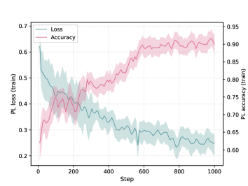
(a) Training PL loss and accuracy on held-out domain: book.

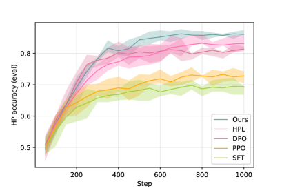
(b) Evaluation PL accuracy on held-out domain: book.

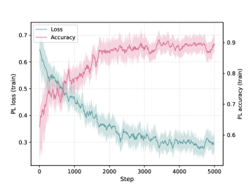
(c) Training PL loss and accuracy on held-out domains: ac&an&ba.

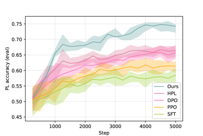
(d) Evaluation PL accuracy on held-out domains: ac&an&ba.

Figure 2: PL accuracy $\mathcal{A}_{\rm PL}$ against the training steps.

Preference data from the test distributions is utilized for evaluation. Specifically, we examine the optimization of the outer objective against the training steps, as depicted in Figure 2. Figure 2 (a) and (c) demonstrate that the PL loss $\ell_{\rm PL}$ decreases rapidly within the initial 600 steps for the controlled sentiment generation task and within the initial 3,000 steps for the knowledge answer generation task, respectively. Subsequently, the PL loss reaches a low value for both tasks, exhibiting only minor fluctuations. The PL accuracy $\mathcal{A}_{\rm PL}$ increases in the opposite trend to the PL loss and eventually surpasses $0.9$ for both tasks. This indicates that our method is effective in conducting in-distribution preference learning. To compare various methods for out-of-distribution preference learning, Figure 2 (b) and (d) depict the PL accuracy $\mathcal{A}_{\rm PL}$ on the evaluation set of test distributions for controlled sentiment generation and knowledge answer generation, respectively. In comparison to the SFT baseline, other methods utilize preference data for training, resulting in higher PL accuracy for both tasks. Moreover, our method optimizes a bilevel optimization objective for out-of-distribution preference learning, significantly outperforming other methods by achieving a PL accuracy of $0.86$ for controlled sentiment generation and $0.75$ for knowledge answer generation.

4.3 Evaluation with a Learned RM

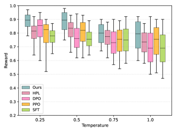
(a) Held-out domain: book.

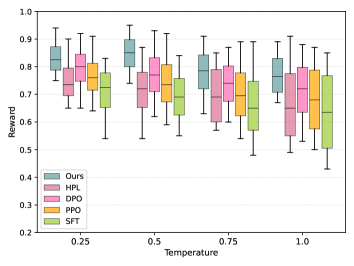
(b) Held-out domain: dvd.

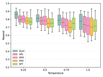
(c) Held-out domain: electronics.

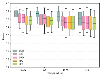
(d) Held-out domain: kitchen.

Figure 3: Reward on the amazon review sentiment generation.

Following the approach of Rafailov et al. (2024), we employ a learned reward model to evaluate preference learning in controlled sentiment generation. Specifically, we train a RoBERTa_LARGE-based sentiment classifier to serve as the reference reward function across four domains of the amazon review dataset. As depicted in Figure 3, we compare various out-of-distribution preference learning methods across four held-out domains, using different temperatures ranging from ${0.25,0.5,0.75,1.0}$ to control the randomness of generation. The results for each temperature represent the average of three repetitions of generation. From Figure 3, it is observed that as the temperature increases from $0.25$ to $1.0$, the variances of rewards for all methods tend to increase across the four held-out domains. Despite the wide range of rewards observed for all methods, our method consistently outperforms other baselines in terms of median reward across all temperatures. This demonstrates the effectiveness of our proposed approach in optimizing a general reward function for out-of-distribution preference learning.

4.4 Evaluation with GPT-4 Judgement

target domain	ac,an,ba				ca,cu,do				ne,hi,hr
	ac	an	ba	avg.	ca	cu	do	avg.	ne	hi	hr	avg.
Base Model	0.153	0.234	0.198	0.195	0.225	0.124	0.181	0.177	0.176	0.206	0.134	0.132
Sft	0.587	0.543	0.495	0.542	0.478	0.521	0.576	0.525	0.578	0.525	0.456	0.520
Ppo (tr)	0.646	0.586	0.557	0.596	0.507	0.604	0.558	0.556	0.660	0.557	0.502	0.573
Ppo (tr+te)	0.682	0.594	0.567	0.614	0.557	0.614	0.583	0.585	0.672	0.587	0.536	0.598
Dpo	0.657	0.554	0.565	0.592	0.525	0.537	0.612	0.558	0.648	0.506	0.527	0.560
Hpl	0.536	0.497	0.624	0.552	0.556	0.625	0.542	0.574	0.682	0.486	0.478	0.549
our method	0.724	0.607	0.724	0.685	0.686	0.687	0.702	0.692	0.686	0.652	0.586	0.642
target domain	phi,phy,sci				scif,so,ve				ch,ex,le
	phi	phy	sci	avg.	scif	so	ve	avg.	ch	ex	le	avg.
Base Model	0.152	0.237	0.167	0.185	0.188	0.193	0.215	0.199	0.203	0.113	0.124	0.147
Sft	0.467	0.506	0.456	0.476	0.526	0.497	0.502	0.508	0.546	0.487	0.568	0.534
Ppo (tr)	0.568	0.545	0.563	0.558	0.602	0.507	0.478	0.529	0.654	0.604	0.625	0.628
Ppo (tr+te)	0.601	0.552	0.597	0.583	0.640	0.528	0.601	0.590	0.647	0.654	0.639	0.647
Dpo	0.507	0.582	0.557	0.549	0.580	0.527	0.554	0.554	0.636	0.452	0.657	0.582
Hpl	0.342	0.478	0.572	0.467	0.582	0.486	0.557	0.542	0.486	0.627	0.586	0.566
our method	0.604	0.686	0.724	0.671	0.656	0.567	0.652	0.625	0.672	0.680	0.749	0.700

Table 3: GPT-4 evaluation of win rate on the knowledge answer generation. We format the best, the second best and worse than SFT results.

Building on previous work, we utilize GPT-4 to evaluate whether an answer generated by the model is more correct and useful compared to the preferred response from the knowledge answer generation dataset. We then assess the win rates of all methods against the preferred answers in the dataset. As depicted in Table 3, all fine-tuning methods significantly outperform the base model of Flan-T5 XXL. This highlights the importance of fine-tuning a pretrained language model with supervised data for the knowledge answer generation task. In comparison to the Sft baseline, the other methods utilize human preference data for further fine-tuning, resulting in better win rates across all held-out domains. Compared to Ppo (tr), Ppo (tr+te) utilizes supervised data from test distributions for fine-tuning and achieves higher average win rates for each experiment, demonstrating the effectiveness of using in-distribution data for fine-tuning a language model. However, all baselines including Ppo, Dpo, and Hpl are constrained by direct training on in-distribution preference data, and thus can only learn in-distribution preference information. In contrast, we employ a bilevel optimization approach to learn a general reward function, which can be applied to out-of-distribution policy fine-tuning. Consequently, our method achieves the best results across all out-of-distribution experiments.

4.5 Effects of $\beta$ on Reward Learning

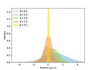
(a) Reward on meta-test set of book.

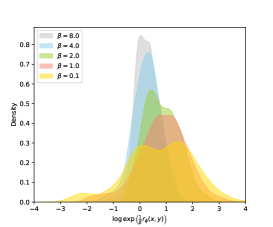
(b) logarithm of combination term on meta-test set of book.

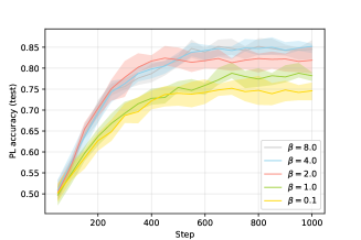
(c) PL accuracy on test set of book.

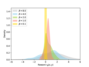
(d) Reward on meta-test set of ac,an,ba.

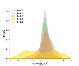
(e) logarithm of combination term on meta-test set of ac,an,ba.

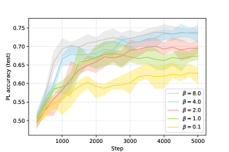
(f) PL accuracy on test set of ac,an,ba.

Figure 4: The effects of reward learning w.r.t. the reward controlling factor $\beta$.

Figure 4 illustrates our investigation into various values of $\beta\in{0.1,1.0,2.0,4.0,8.0}$ for reward learning. From Figures 4 (a) and (d), it is evident that when the reward controlling factor is too small, such as $\beta=0.1$, the reward distribution becomes very sharp and approaches $0$, providing limited information for policy fine-tuning. As $\beta$ increases, the reward distribution becomes flatter, which better represents the preferences of inputs for guiding policy fine-tuning. Additionally, we explore the learning of the combination term $\exp\left(\frac{1}{\beta}r_{\phi}(x,y)\right)$ for cross-entropy in the inner objective. Figures 4 (b) and (e) demonstrate that as $\beta$ increases, the distribution of the combination term approaches a standard normal distribution, facilitating faster convergence of policy fine-tuning. Furthermore, we examine how $\beta$ influences preference learning by presenting the preference learning accuracy against the training steps for various values of $\beta$ in Figures 4 (c) and (f). We observe that for each value of $\beta$, as the number of training steps increases, the preference learning accuracy improves and eventually converges to a high plateau. Moreover, a larger value of $\beta$ yields better preference learning accuracy for both tasks. The experimental findings align with the theoretical result of Theorem 1, suggesting that a larger number of iterations $K$ and a larger value of $\beta$ contribute to the algorithm’s convergence to a more accurate stationary point.

5 Conclusion

Preference learning (PL) is a powerful framework for training language models to align with human values. Instead of discretely training a reward model solely for in-distribution PL, this work investigated an out-of-distribution (OOD) PL algorithm. The aim is to improve the generalization of reward modeling for aligning a language policy with human preferences across various test distributions. To address OOD PL, we proposed a meta-learning approach conducted through a bilevel optimization algorithm. The outer objective aims to align the predicted probability generated by the language policy with human preferences, while the inner objective focuses on performing regularized policy optimization with the learned reward model. As a result, when encountering a novel test distribution, fine-tuning the language policy using only supervised data can achieve alignment with human preferences. By deriving the inner objective, we revised the regularization term in previous work on RLHF by incorporating consideration of the target distribution to mitigate policy drift. Additionally, we employed a parameter estimation approach to reduce the RL objective to a regression problem for more efficient training. We derived an upper bound for the convergence rate of reward model learning using the proposed bilevel optimization algorithm. This bound demonstrates significant relationships with the number of outer-loop iterations and the controlling factor of reward modeling. We conducted experiments on both controlled sentiment generalization and knowledge answer generation. Evaluation with preference data demonstrates that the generalized reward modeling achieved by our meta-learning approach effectively guides policy learning to align with human preferences. Evaluation on sentiment generation with a learned reward model indicates that our method achieves superior rewards compared to other OOD PL baselines across four domains. Evaluation using GPT-4 judgment demonstrates that our method outperforms a range of strong baselines, achieving the highest win rate across 16 held-out domains.

Appendix A Parameter Estimation for Policy Learning

Based on the objective function of policy in Eq. (9), we have

$$\mathop{\arg\max}_{\pi}\mathbb{E}_{x\sim\mathcal{D}}\left[\mathbb{E}_{y\sim\pi(\cdot|x)}\left[r_{\phi}(x,y)\right]-\beta\mathrm{D}_{\rm KL}\left(\pi(\cdot|x)||\hat{\mu}(\cdot|x)\right)\right]$$

$$=\mathop{\arg\max}_{\pi}\int_{x}\mathcal{D}(x)\left(\int_{y}\pi(y|x)r_{\phi}(x,y)dy-\beta\mathrm{D}_{\rm KL}\left(\pi(\cdot|x)||\hat{\mu}(\cdot|x)\right)\right)dx$$

Then, we can formulate the following constrained policy optimization problem,

$$\mathop{\arg\max}_{\pi} \int_{x}\mathcal{D}(x)\left(\int_{y}\pi(y|x)r_{\phi}(x,y)dy-\beta\mathrm{D}_{\rm KL}\left(\pi(\cdot|x)||\hat{\mu}(\cdot|x)\right)\right)dx$$

$${\rm s.t.}\ \int_{y}\pi(y|x)dy=1,\quad\forall x$$

Next, we can form the Lagrangian,

$$\mathcal{L}(\pi,\alpha)=\int_{x}\mathcal{D}(x)\left(\int_{y}\pi(y|x)r_{\phi}(x,y)dy-\beta\mathrm{D}_{\rm KL}\left(\pi(\cdot|x)||\hat{\mu}(\cdot|x)\right)\right)dx+\int_{x}\alpha_{x}\left(1-\int_{y}\pi(y|x)dy\right)dx,$$

with $\alpha=\{\alpha_{x}:\forall x\in\mathcal{X}\}$ corresponding to the Lagrange multipliers. Now, we can differentiate $\mathcal{L}(\pi,\alpha)$ w.r.t. $\pi(y|x)$ as

$$\frac{\partial\mathcal{L}(\pi,\alpha)}{\partial\pi(y|x)}= \frac{\partial}{\partial\pi(y|x)}\int_{x}\int_{y}\pi(y|x)\left(\mathcal{D}(x)\left(r_{\phi}(x,y)-\beta\log\pi(y|x)+\beta\log\hat{\mu}(y|x)\right)-\alpha_{x}\right)dy+\alpha_{x}dx$$

$$= \int_{x}\int_{y}\frac{\partial}{\partial\pi(y|x)}\pi(y|x)\left(\mathcal{D}(x)\left(r_{\phi}(x,y)-\beta\log\pi(y|x)+\beta\log\hat{\mu}(y|x)\right)-\alpha_{x}\right)dydx$$

$$= \int_{x}\int_{y}\left(\mathcal{D}(x)r_{\phi}(x,y)-\beta\mathcal{D}(x)\log\pi(y|x)-\beta\mathcal{D}(x)+\beta\mathcal{D}(x)\log\hat{\mu}(y|x)-\alpha_{x}\right)dydx$$

Setting the above integrated term to zero, we can obtain a sufficient condition on $\frac{\partial\mathcal{L}(\pi,\alpha)}{\partial\pi(y|x)}=0$,

$$\pi_{*}(y|x)=\hat{\mu}(y|x)\exp\left(\frac{1}{\beta}r_{\phi}(x,y)\right)\exp\left(-\frac{\alpha_{x}}{\beta\mathcal{D}(x)}-1\right),\quad\forall y\forall x$$ (27)

Besides, the strict negativeness of the sencond-order partial derivative of $\mathcal{L}(\pi,\alpha)$ is shown by

$$\frac{\partial^{2}\mathcal{L}(\pi,\alpha)}{\partial[\pi(y|x)]^{2}}=\int_{x}\int_{y}-\frac{\beta\mathcal{D}(x)}{\pi(y|x)}dydx<0,$$

since $\beta,\mathcal{D}(x),\pi(y|x)>0$. This indicates the strict concaveness of $\mathcal{L}(\pi,\alpha)$. Therefore, Eq. (27) indicates a global optimization solution $\pi_{*}=\mathop{\arg\max}_{\pi}\mathcal{L}(\pi,\alpha)$.

Since $\int_{y}\pi^{*}(y|x)dy=1$, the second exponential term can be rewritten as a partition function $Z(x)$ that normalizes the conditional action distribution,

$$Z(x)=\exp\left(\frac{\alpha_{x}}{\beta\mathcal{D}(x)}+1\right)=\int_{y}\hat{\mu}(y|x)\exp\left(\frac{1}{\beta}r_{\phi}(x,y)\right)dy$$

The optimal policy is therefore given by,

$$\pi^{*}(y|x)=\frac{1}{Z(x)}\hat{\mu}(y|x)\exp\left(\frac{1}{\beta}r_{\phi}(x,y)\right),\quad\forall y\forall x$$ (28)

To obtain such a global optimization solution for the policy, we use a parameter estimation method, i.e., using a machine learning method to train a parameter estimated policy $\pi_{\theta}$ close to the globally optimal solution $\pi^{*}$ of Eq. (28) by solving the following supervised regression problem:

$$\mathop{\arg\min}_{{\theta}}\mathbb{E}_{x\sim\mathcal{D}}\left[\mathrm{D}_{\rm KL}\left(\pi^{*}(\cdot|x)||\pi_{\theta}(\cdot|x)\right)\right]$$

$$= \mathop{\arg\min}_{{\theta}}\mathbb{E}_{x\sim\mathcal{D}}\left[\mathrm{D}_{\rm KL}\left(\frac{1}{Z(x)}\hat{\mu}(y|x)\exp\left(\frac{1}{\beta}r_{\phi}(x,y)\right)\bigg{\|}\pi_{\theta}(\cdot|x)\right)\right]$$

$$= \mathop{\arg\min}_{\theta}-\mathbb{E}_{x\sim\mathcal{D}}\mathbb{E}_{y\sim\hat{\mu}(y|x)}\left[\log\pi_{\theta}(y|x)\exp\left(\frac{1}{\beta}r_{\phi}(x,y)\right)\right]$$

Appendix B Proof of Proposition 1

Based on the formulation of outer objective $\ell_{\rm PL}$ in Eq. (7), we have for any $k\in\{0,1,2,\ldots,K-1\}$ and the input data $(x_{k},y_{k},y^{\prime}_{k})$,

$$\frac{\partial\ell_{\rm PL}({\phi_{k}},{\theta_{k,D}})}{\partial{\phi}_{k}} =-\frac{\partial}{\partial{\phi}_{k}}\log\sigma\left(\log\pi_{\theta_{k,D}}(y_{k}|x_{k})-\log\pi_{\theta_{k,D}}(y^{\prime}_{k}|x_{k})\right)$$ (29)

$$=-\frac{\partial{\theta}_{k,D}}{\partial{\phi}_{k}}\left(\nabla_{{\theta}}\log\pi_{\theta_{k,D}}(y_{k}|x_{k})-\nabla_{{\theta}}\log\pi_{{\theta}_{k,D}}(y^{\prime}_{k}|x_{k})\right)$$ (30)

Based on the formulation of inner objective $\ell_{\rm FT}$ in Eq. (10), the iterative update for any $t\in\{0,1.2,\ldots,D-1\}$ based on the input data $(x_{k,y},y_{k,t})$ takes the form

$${\theta}_{k,t+1}= {\theta}_{k,t}-\alpha\nabla_{{\theta}}\ell_{\rm FT}({\phi_{k}},\pi_{{k,t}})$$

$$= {\theta}_{k,t}+\alpha\nabla_{\theta}\left(\log\pi_{\theta_{k,t}}(y_{k,t}|x_{k,t})\exp\left(\frac{1}{\beta}r_{\phi_{k}}(x_{k,t},y_{k,t})\right)\right)$$

$$= {\theta}_{k,t}+\alpha\nabla_{\theta}\log\pi_{\theta_{k,t}}(y_{k,t}|x_{k,t})\exp\left(\frac{1}{\beta}r_{\phi_{k}}(x_{k,t},y_{k,t})\right)$$

Then, we have

$$\frac{\partial{\theta}_{k,t+1}}{\partial{\phi_{k}}}=\frac{\partial{\theta}_{k,t}}{\partial{\phi}_{k}} +\alpha\frac{\partial{\theta}_{k,t}}{\partial{\phi}_{k}}\nabla^{2}_{{\theta}}\log\pi_{\theta_{k,t}}(y_{k,t}|x_{k,t})\exp\left(\frac{1}{\beta}r_{\phi_{k}}(x_{k,t},y_{k,t})\right)$$

$$+\frac{\alpha}{\beta}\nabla_{{\theta}}\log\pi_{\theta_{k,t}}(y_{k,t}|x_{k,t})\exp\left(\frac{1}{\beta}r_{\phi_{k}}(x_{k,t},y_{k,t})\right)$$

To simplify the presentation, let $R^{k,t}:=\exp\left(\frac{1}{\beta}r_{\phi_{k}}(x_{k,t},y_{k,t})\right)$, $F^{k,t}:=\log\pi_{\theta_{k,t}}(y_{k,t}|x_{k,t})$ and $\nabla:=\nabla_{{\theta}}$, we have

$$\frac{\partial{\theta}_{k,t+1}}{\partial{\phi}_{k}}= \frac{\partial{\theta}_{k,t}}{\partial{\phi}_{k}}\left(I+\alpha R^{k,t}\nabla^{2}F^{k,t}\right)+\frac{\alpha}{\beta}R^{k,t}\nabla F^{k,t}$$

Telescoping the above equality over $t$ from $1$ to $D$ yields

$$\begin{split}\frac{\partial{\theta}_{k,D}}{\partial{\phi_{k}}}=&\frac{\partial{\theta}_{k,0}}{\partial{\phi_{k}}}\prod_{t=0}^{D-1}\left(I+\alpha R^{k,t}\nabla^{2}F^{k,t}\right)+\frac{\alpha}{\beta}\sum_{t=0}^{D-1}R^{k,t}\nabla F^{k,t}\prod_{j=t+1}^{D-1}\left(I+\alpha R^{k,t}\nabla^{2}F^{k,t}\right)\\ =&\frac{\alpha}{\beta}\sum_{t=0}^{D-1}R^{k,t}\nabla F^{k,t}\prod_{j=t+1}^{D-1}\left(I+\alpha R^{k,t}\nabla^{2}F^{k,t}\right),\end{split}$$ (31)

where the second equation follows from the fact that $\frac{\partial{\theta}_{k,0}}{\partial\phi_{k}}=0$. Combining Eq. (29) and Eq. (31) finishes the proof.

Appendix C Supporting Lemmas

Lemma 1.

Based on Assumption 1, 2 and 3, $\mathcal{L}_{\rm FT}(\phi,\theta)$ is $\frac{BL}{\exp\beta}$-smoothness and $\frac{b\mu}{\exp\beta}$-strong convexity w.r.t. $\theta$.

Proof.

The $\frac{BL}{\exp\beta}$-smoothness of $\mathcal{L}_{\rm FT}(\phi,\theta)$ follows from

$$\left\|\nabla_{\theta}\mathcal{L}_{\rm FT}(\phi,\theta)-\nabla_{\theta}\mathcal{L}_{\rm FT}(\phi,\theta^{\prime})\right\|=\left\|\mathbb{E}_{z}\left[\nabla_{\theta}\ell_{\rm FT}(\phi,\theta;z)\right]-\mathbb{E}_{z}\left[\ell_{\rm FT}(\phi,\theta^{\prime};z)\right]\right\|$$

$$\overset{(i)}{\leq} \mathbb{E}_{z}\left[\left\|\nabla_{\theta}\log\pi_{\theta^{\prime}}(y|x)\exp\left(\frac{1}{\beta}r_{\phi}(x,y)\right)-\nabla_{\theta}\log\pi_{\theta}(y|x)\exp\left(\frac{1}{\beta}r_{\phi}(x,y)\right)\right\|\right]$$

$${=} \mathbb{E}_{z}\left[\exp\left(\frac{1}{\beta}r_{\phi}(x,y)\right)\left\|\nabla_{\theta}\log\pi_{\theta^{\prime}}(y|x)-\nabla_{\theta}\log\pi_{\theta}(y|x)\right\|\right]$$

$$\overset{(ii)}{\leq} \frac{BL}{\exp\beta}\|\theta-\theta^{\prime}\|,$$

where $(i)$ follows from Jensen’s inequality and the definition of $\mathcal{L}_{\rm FT}(\phi,\theta)$ $(ii)$ follows from the $L$-smoothness of $-\log\pi_{\theta}(y|x)$ in Assumption 2 and the $B$-boundness of $\exp r_{\phi}(x,y)$ in Asssumption 3.

The $\frac{b\mu}{\exp\beta}$-strong convexity of $\mathcal{L}_{\rm FT}(\phi,\theta)$ follows from

$$\left\langle\nabla_{\theta}\mathcal{L}_{\rm FT}(\phi,\theta)-\nabla_{\theta}\mathcal{L}_{\rm FT}(\phi,\theta^{\prime}),\theta-\theta^{\prime}\right\rangle=\mathbb{E}_{z}\left[\left\langle\nabla_{\theta}\ell_{\rm FT}(\phi,\theta)-\nabla_{\theta}\ell_{\rm FT}(\phi,\theta^{\prime}),\theta-\theta^{\prime}\right\rangle\right]$$

$$\overset{(i)}{=} \mathbb{E}_{z}\left[\left\langle\nabla_{\theta}\log\pi_{\theta^{\prime}}(y|x)\exp\left(\frac{1}{\beta}r_{\phi}(x,y)\right)-\nabla_{\theta}\log\pi_{\theta}(y|x)\exp\left(\frac{1}{\beta}r_{\phi}(x,y)\right),\theta-\theta^{\prime}\right\rangle\right]$$

$$\overset{(ii)}{\geq} \mathbb{E}_{z}\left[\exp\left(\frac{1}{\beta}r_{\phi}(x,y)\right)\left\|\theta-\theta^{\prime}\right\|^{2}\right]\overset{(iii)}{\geq}\frac{b\mu}{\exp\beta}\|\theta-\theta^{\prime}\|^{2},$$

where $(i)$ follows from the definition of $\mathcal{L}_{\rm FT}(\phi,\theta)$, $(ii)$ follows from the $\mu$-strong convexity of $-\log\pi_{\theta}(y|x)$ in Assumption 1, $(iii)$ follows from the boundness assumption of $\exp(r_{\theta}(x,y))$ in Assumption 3.

∎

Lemma 2.

Based on Assumption 2 and 3, we have the Lipschitz properties of $\nabla_{\phi}\nabla_{\theta}\ell_{\rm FT}(\phi,\theta)$ and $\nabla_{\theta}^{2}\ell_{\rm FT}(\phi,\theta)$,

$$\left\|\nabla_{\phi}\nabla_{\theta}\ell_{\rm FT}(\phi,\theta)-\nabla_{\phi}\nabla_{\theta}\ell_{\rm FT}(\phi,\theta^{\prime})\right\| \leq\frac{BTL}{\beta\exp\beta}\|\theta-\theta^{\prime}\|$$ (32)

$$\left\|\nabla_{\theta}^{2}\ell_{\rm FT}(\phi,\theta)-\nabla_{\theta}^{2}\ell_{\rm FT}(\phi,\theta^{\prime})\right\| \leq\frac{B\rho}{\exp\beta}\|\theta-\theta^{\prime}\|$$ (33)

Proof.

Based on the definition of $\ell_{\rm FT}(\phi,\theta)$, we have for any $(x,y)$ and any $\theta,\theta^{\prime}$,

$$\left\|\nabla_{\phi}\nabla_{\theta}\ell_{\rm FT}(\phi,\theta)-\nabla_{\phi}\nabla_{\theta}\ell_{\rm FT}(\phi,\theta^{\prime})\right\|$$

$$= \left\|\frac{1}{\beta}\exp\left(\frac{r_{\phi}(x,y)}{\beta}\right)\nabla_{\phi}r_{\phi}(x,y)\nabla_{\theta}\log\pi_{\theta^{\prime}}(y|x)-\frac{1}{\beta}\exp\left(\frac{r_{\phi}(x,y)}{\beta}\right)\nabla_{\phi}r_{\phi}(x,y)\nabla_{\theta}\log\pi_{\theta}(y|x)\right\|$$

$$\overset{(i)}{\leq} \left\|\frac{1}{\beta}\exp\left(\frac{r_{\phi}(x,y)}{\beta}\right)\nabla_{\phi}r_{\phi}(x,y)\right\|\left\|\nabla_{\theta}\log\pi_{\theta^{\prime}}(y|x)-\nabla_{\theta}\log\pi_{\theta}(y|x)\right\|$$

$$\overset{(ii)}{\leq} \frac{BTL}{\beta\exp\beta}\left\|\theta-\theta^{\prime}\right\|,$$

where $(i)$ follows from Cauchy-Schwarz inequality and $(ii)$ follows from Assumption 2 and 3.

Similarly, we also have

$$\left\|\nabla_{\theta}^{2}\ell_{\rm FT}(\phi,\theta)-\nabla_{\theta}^{2}\ell_{\rm FT}(\phi,\theta^{\prime})\right\|$$

$$= \left\|\nabla_{\theta}^{2}\log\pi_{\theta^{\prime}}(y|x)\exp\left(\frac{r_{\phi}(x,y)}{\beta}\right)-\nabla_{\theta}^{2}\log\pi_{\theta}(y|x)\exp\left(\frac{r_{\phi}(x,y)}{\beta}\right)\right\|$$

$$\leq \exp\left(\frac{r_{\phi}(x,y)}{\beta}\right)\left\|\nabla_{\theta}^{2}\log\pi_{\theta^{\prime}}(y|x)-\nabla_{\theta}^{2}\log\pi_{\theta}(y|x)\right\|$$

$$\overset{(i)}{\leq} \frac{B\rho}{\exp\beta}\|\theta-\theta^{\prime}\|,$$

where $(i)$ follows from Assumption 2 and 3. ∎

Appendix D Proof of the Main Theorem

D.1 Useful Lemmas

Lemma 3.

For any $k\in\{0,1,2,\ldots,K-1\}$, we have

$$\begin{split}&\mathbb{E}\left[\left\|\frac{\partial\mathcal{L}_{\rm PL}({\phi_{k}},{\theta_{k,D}})}{\partial\phi_{k}}-\frac{\partial\mathcal{L}_{\rm PL}({\phi_{k}},{\theta_{*}})}{\partial\phi_{k}}\right\|^{2}\right]\\ {\leq}&8M^{2}\left(3\left(1-\frac{\alpha b\mu}{\exp\beta}\right)^{2}\right)^{D}\frac{T^{2}}{\beta^{2}}\left(\frac{M^{2}}{L^{2}}+\left\|\theta_{0}-\theta_{*}\right\|^{2}\right)\\ &+8M^{2}\left(\frac{\alpha^{2}\sigma^{2}T^{2}}{\beta^{2}}+6\alpha^{2}\sigma_{1}^{2}+\frac{6M^{2}T^{2}}{\beta^{2}L^{2}}\sigma_{2}^{2}\right)\sum_{t=0}^{D-1}\left(3\left(1-\frac{\alpha b\mu}{\exp\beta}\right)^{2}\right)^{t}\end{split}$$ (34)

Proof.

Based on $\frac{\partial\mathcal{L}_{\rm PL}(\phi_{k},\theta_{*})}{\partial\phi_{k}}=\frac{\partial\mathcal{L}_{\rm PL}(\theta_{*})}{\partial\phi_{k}}=\frac{\partial\theta_{*}}{\partial\phi_{k}}\nabla_{{\theta}}\mathcal{L}_{\rm PL}(\phi_{k},\theta_{*})$, and similarly $\frac{\partial\mathcal{L}_{\rm PL}(\phi_{k},\theta_{k,D})}{\partial\phi_{k}}=\frac{\partial\theta_{k,D}}{\partial\phi_{k}}\nabla_{{\theta}}\mathcal{L}_{\rm PL}({\phi_{k}},{\theta_{k,D}})$, using the triangle inequality and Jensen’s inequality, we have

$$\left\|\frac{\partial\mathcal{L}_{\rm PL}({\phi_{k}},{\theta_{k,D}})}{\partial\phi_{k}}-\frac{\partial\mathcal{L}_{\rm PL}({\phi_{k}},{\theta_{*}})}{\partial\phi_{k}}\right\|=\left\|\frac{\partial{\theta_{k,D}}}{\partial\phi_{k}}\nabla_{{\theta}}\mathcal{L}_{\rm PL}({\phi_{k}},{\theta_{k,D}})-\frac{\partial{\theta_{*}}}{\partial\phi_{k}}\nabla_{{\theta}}\mathcal{L}_{\rm PL}({\phi_{k}},{\theta_{*}})\right\|$$

$$\leq \left\|\frac{\partial{\theta_{k,D}}}{\partial\phi_{k}}-\frac{\partial{\theta_{*}}}{\partial\phi_{k}}\right\|\left\|\nabla_{{\theta}}\mathcal{L}_{\rm PL}({\phi_{k}},{\theta_{k,D}})\right\|+\left\|\frac{\partial{\theta_{*}}}{\partial\phi_{k}}\right\|\left\|\nabla_{{\theta}}\mathcal{L}_{\rm PL}({\phi_{k}},{\theta_{k,D}})-\nabla_{{\theta}}\mathcal{L}_{\rm PL}({\phi_{k}},{\theta_{*}})\right\|$$

$$\overset{(i)}{\leq} 2M\left\|\frac{\partial{\theta_{k,D}}}{\partial\phi_{k}}-\frac{\partial{\theta_{*}}}{\partial\phi_{k}}\right\|+2L\left\|\frac{\partial{\theta_{*}}}{\partial\phi_{k}}\right\|\|\theta_{k,D}-{\theta_{*}}\|$$

where $(i)$ using Assumption 2 and the fact that

$$\|\mathcal{L}_{\rm PL}({\phi_{k}},{\theta_{k,D}})\| =\left\|\mathbb{E}\left[\nabla\log\pi_{\theta_{k,D}}(y|x)-\nabla\log\pi_{\theta_{k,D}}(y^{\prime}|x)\right]\right\|$$

$$\leq\mathbb{E}\left[\left\|\nabla\log\pi_{\theta_{k,D}}(y|x)\right\|\right]+\mathbb{E}\left[\left\|\nabla\log\pi_{\theta_{k,D}}(y^{\prime}|x)\right\|\right]\leq 2M;$$

$$\left\|\nabla_{{\theta}}\mathcal{L}_{\rm PL}({\phi_{k}},{\theta_{k,D}})-\nabla_{{\theta}}\mathcal{L}_{\rm PL}({\phi_{k}},{\theta_{*}})\right\|$$

$$= \left\|\mathbb{E}\left[\nabla\log\pi_{\theta_{k,D}}(y|x)-\nabla\log\pi_{\theta_{k,D}}(y^{\prime}|x)\right]-\mathbb{E}\left[\nabla\log\pi_{\theta_{*}}(y|x)-\nabla\log\pi_{\theta_{*}}(y^{\prime}|x)\right]\right\|$$

$$\leq \mathbb{E}\left[\left\|\nabla\log\pi_{\theta_{k,D}}(y|x)-\nabla\log\pi_{\theta_{*}}(y|x)\right\|\right]+\mathbb{E}\left[\left\|\nabla\log\pi_{\theta_{k,D}}(y^{\prime}|x)-\nabla\log\pi_{\theta_{*}}(y^{\prime}|x)\right\|\right]$$

$$\leq 2L\|\theta_{k,D}-{\theta_{*}}\|,$$

based on the optimality of ${\theta_{*}}$, we have $\nabla_{{\theta}}\mathcal{L}_{\rm FT}({\phi_{k}},{\theta_{*}})=0$, which in conjunction the implicit differentiation theorem, yields

$$\nabla_{\phi}\nabla_{{\theta}}\mathcal{L}_{\rm FT}({\phi_{k}},{\theta_{*}})+\frac{\partial{\theta_{*}}}{\partial\phi_{k}}\nabla_{{\theta}}^{2}\mathcal{L}_{\rm FT}({\phi_{k}},{\theta_{*}})=0,$$ (35)

then, we have

$$\left\|\frac{\partial{\theta_{*}}}{\partial\phi_{k}}\right\|= \left\|\nabla_{\phi}\nabla_{{\theta}}\mathcal{L}_{\rm FT}({\phi_{k}},{\theta_{*}})\left[\nabla_{{\theta}}^{2}\mathcal{L}_{\rm FT}({\phi_{k}},{\theta_{*}})\right]^{-1}\right\|$$

$${=} \left\|\mathbb{E}\left[\frac{1}{\beta}\exp\left(\frac{1}{\beta}r_{\phi_{k}}(x,y)\right)\nabla_{{\theta}}\log\pi_{\theta_{*}}(y|x)\nabla_{\phi}r_{\phi_{k}}(x,y)\right]\mathbb{E}\left[\exp\left(\frac{1}{\beta}r_{\phi_{k}}(x,y)\right)\nabla_{{\theta}}^{2}\log\pi_{\theta_{*}}(y|x)\right]^{-1}\right\|$$

$$\overset{(i)}{\leq} \frac{1}{\beta}\mathbb{E}\left[\left\|\nabla_{{\theta}}\log\pi_{\theta_{*}}(y|x)\right\|\left\|\nabla_{\phi}r_{\phi_{k}}(x,y)\right\|\right]\mathbb{E}\left[\left\|\nabla^{2}_{{\theta}}\log\pi_{\theta_{*}}(y|x)\right\|^{-1}\right]\overset{(ii)}{\leq}\frac{MT}{\beta L},$$

where $(i)$ follows from Cauchy-Schwarz’s inequality and Jensen’s inequality, $(ii)$ follows from Assumption 2.

Thus, we have

$$\left\|\frac{\partial\mathcal{L}_{\rm PL}({\phi_{k}},{\theta_{k,D}})}{\partial\phi_{k}}-\frac{\partial\mathcal{L}_{\rm PL}({\phi_{k}},{\theta_{*}})}{\partial\phi_{k}}\right\|\leq 2M\left\|\frac{\partial{\theta_{k,D}}}{\partial\phi_{k}}-\frac{\partial{\theta_{*}}}{\partial\phi_{k}}\right\|+2L\left\|\frac{\partial{\theta_{*}}}{\partial\phi_{k}}\right\|\|\theta_{k,D}-{\theta_{*}}\|$$

$$\leq 2M\left\|\frac{\partial{\theta_{k,D}}}{\partial\phi_{k}}-\frac{\partial{\theta_{*}}}{\partial\phi_{k}}\right\|+\frac{2MT}{\beta}\|\theta_{k,D}-{\theta_{*}}\|$$

Taking expectation on both sides and using Lemma 4, we have Eq. (34).

∎

Lemma 4.

For any $k\in\{0,1,2,\ldots,K-1\}$,

$$\begin{split}&\mathbb{E}\left[\left\|\frac{\partial\theta_{k,D}}{\partial\phi_{k}}-\frac{\partial\theta_{*}}{\partial\phi_{k}}\right\|^{2}\right]+\frac{T^{2}}{\beta^{2}}\mathbb{E}\left[\left\|\theta_{k,D}-\theta_{*}\right\|^{2}\right]\\ \leq&\left(3\left(1-\frac{\alpha b\mu}{\exp\beta}\right)^{2}\right)^{D}\frac{T^{2}}{\beta^{2}}\left(\frac{M^{2}}{L^{2}}+\left\|\theta_{0}-\theta_{*}\right\|^{2}\right)\\ &+\left(\frac{\alpha^{2}\sigma^{2}T^{2}}{\beta^{2}}+6\alpha^{2}\sigma_{1}^{2}+\frac{6M^{2}T^{2}}{\beta^{2}L^{2}}\sigma_{2}^{2}\right)\sum_{t=0}^{D-1}\left(3\left(1-\frac{\alpha b\mu}{\exp\beta}\right)^{2}\right)^{t}\end{split}$$ (36)

Proof.

Based on the updating rule of SGD $\theta_{k,t+1}=\theta_{k,t}-\alpha\nabla_{{\theta}}\ell_{\rm FT}({\phi_{k}},{\theta_{k,t}};z_{k,t})$, for any $t\in\{0,1,2,\ldots,D-1\}$, we have

$$\frac{\partial\theta_{k,t+1}}{\partial\phi_{k}}=\frac{\partial\theta_{k,t}}{\partial\phi_{k}}-\alpha\left(\nabla_{\phi}\nabla_{{\theta}}\ell_{\rm FT}({\phi_{k}},{\theta_{k,t}};z_{k,t})-\frac{\partial\theta_{k,t}}{\partial\phi_{k}}\nabla^{2}_{{\theta}}\ell_{\rm FT}({\phi_{k}},{\theta_{k,t}};z_{k,t})\right)$$ (37)

Based on the optimality of ${\theta_{*}}$, we have $\nabla_{{\theta}}\mathcal{L}_{\rm FT}({\phi_{k}},{\theta_{*}})=0$, which in conjunction the implicit differentiation theorem, yields

$$\nabla_{\phi}\nabla_{{\theta}}\mathcal{L}_{\rm FT}({\phi_{k}},{\theta_{*}})+\frac{\partial{\theta_{*}}}{\partial\phi_{k}}\nabla_{{\theta}}^{2}\mathcal{L}_{\rm FT}({\phi_{k}},{\theta_{*}})=0$$ (38)

Based on Eq. (37) and Eq. (38), we have

$$\frac{\partial\theta_{k,t+1}}{\partial\phi_{k}}-\frac{\partial\theta_{*}}{\partial\phi_{k}}= \frac{\partial\theta_{k,t}}{\partial\phi_{k}}-\frac{\partial\theta_{*}}{\partial\phi_{k}}-\alpha\left(\nabla_{\phi}\nabla_{{\theta}}\ell_{\rm FT}({\phi_{k}},{\theta_{k,t}};z_{k,t})-\frac{\partial\theta_{k,t}}{\partial\phi_{k}}\nabla^{2}_{{\theta}}\ell_{\rm FT}({\phi_{k}},{\theta_{k,t}};z_{k,t})\right)$$

$$+\alpha\left(\nabla_{\phi}\nabla_{{\theta}}\mathcal{L}_{\rm FT}({\phi_{k}},{\theta_{*}})+\frac{\partial{\theta_{*}}}{\partial\phi_{k}}\nabla_{{\theta}}^{2}\mathcal{L}_{\rm FT}({\phi_{k}},{\theta_{*}})\right)$$

$$= \frac{\partial\theta_{k,t}}{\partial\phi_{k}}-\frac{\partial\theta_{*}}{\partial\phi_{k}}-\alpha\left(\nabla_{\phi}\nabla_{{\theta}}\ell_{\rm FT}({\phi_{k}},{\theta_{k,t}};z_{k,t})-\nabla_{\phi}\nabla_{{\theta}}\mathcal{L}_{\rm FT}({\phi_{k}},{\theta_{*}})\right)$$

$$-\alpha\left(\frac{\partial\theta_{k,t}}{\partial\phi_{k}}-\frac{\partial\theta_{*}}{\partial\phi_{k}}\right)\nabla^{2}_{{\theta}}\ell_{\rm FT}({\phi_{k}},{\theta_{k,t}};z_{k,t})$$

$$+\alpha\frac{\partial\theta_{*}}{\partial\phi_{k}}\left(\nabla_{{\theta}}^{2}\mathcal{L}_{\rm FT}({\phi_{k}},{\theta_{*}})-\nabla^{2}_{{\theta}}\ell_{\rm FT}({\phi_{k}},{\theta_{k,t}};z_{k,t})\right)$$

Thus, taking the $\ell_{2}$-norm and expectation, we have

$$\mathbb{E}\left[\left\|\frac{\partial\theta_{k,t+1}}{\partial\phi_{k}}-\frac{\partial\theta_{*}}{\partial\phi_{k}}\right\|^{2}\right]\leq 3\mathbb{E}\left[\left\|I-\alpha\nabla^{2}_{{\theta}}\ell_{\rm FT}({\phi_{k}},{\theta_{k,t}};z_{k,t})\right\|^{2}\left\|\frac{\partial\theta_{k,t}}{\partial\phi_{k}}-\frac{\partial\theta_{*}}{\partial\phi_{k}}\right\|^{2}\right]$$

$$+3\alpha^{2}\mathbb{E}\left[\left\|\nabla_{\phi}\nabla_{{\theta}}\ell_{\rm FT}({\phi_{k}},{\theta_{k,t}};z_{k,t})-\nabla_{\phi}\nabla_{{\theta}}\mathcal{L}_{\rm FT}({\phi_{k}},{\theta_{*}})\right\|^{2}\right]$$

$$+3\alpha^{2}\mathbb{E}\left[\left\|\frac{\partial\theta_{*}}{\partial\phi_{k}}\right\|^{2}\left\|\nabla_{{\theta}}^{2}\mathcal{L}_{\rm FT}({\phi_{k}},{\theta_{*}})-\nabla^{2}_{{\theta}}\ell_{\rm FT}({\phi_{k}},{\theta_{k,t}};z_{k,t})\right\|^{2}\right]$$

$$\overset{(i)}{\leq} 3\left(1-\frac{\alpha b\mu}{\exp\beta}\right)^{2}\mathbb{E}\left[\left\|\frac{\partial\theta_{k,t}}{\partial\phi_{k}}-\frac{\partial\theta_{*}}{\partial\phi_{k}}\right\|^{2}\right]+\frac{6\alpha^{2}B^{2}T^{2}}{\beta^{2}\exp 2\beta}\left(L^{2}+\frac{M^{2}\rho^{2}}{L^{2}}\right)\mathbb{E}\left[\left\|\theta_{k,t}-\theta_{*}\right\|^{2}\right]$$

$$+6\alpha^{2}\sigma_{1}^{2}+\frac{6M^{2}T^{2}}{\beta^{2}L^{2}}\sigma_{2}^{2},$$

where $(i)$ uses Lemma 1 and the fact that

$$\mathbb{E}\left[\left\|\nabla_{\phi}\nabla_{{\theta}}\ell_{\rm FT}({\phi_{k}},{\theta_{k,t}};z)-\nabla_{\phi}\nabla_{{\theta}}\mathcal{L}_{\rm FT}({\phi_{k}},{\theta_{*}})\right\|^{2}\right]\leq 2\mathbb{E}\left[\left\|\nabla_{\phi}\nabla_{{\theta}}\ell_{\rm FT}({\phi_{k}},{\theta_{k,t}};z)-\nabla_{\phi}\nabla_{{\theta}}\ell_{\rm FT}({\phi_{k}},{\theta_{*}};z)\right\|^{2}\right]$$

$$+2\mathbb{E}\left[\left\|\nabla_{\phi}\nabla_{{\theta}}\ell_{\rm FT}({\phi_{k}},{\theta_{*}};z)-\nabla_{\phi}\nabla_{{\theta}}\mathcal{L}_{\rm FT}({\phi_{k}},{\theta_{*}})\right\|^{2}\right]$$

$$\overset{(i)}{\leq} 2\frac{B^{2}T^{2}L^{2}}{\beta^{2}\exp 2\beta}\mathbb{E}\left[\left\|\theta_{k,t}-\theta_{*}\right\|^{2}\right]+2\sigma_{1}^{2};$$

$$\mathbb{E}\left[\left\|\nabla_{{\theta}}^{2}\mathcal{L}_{\rm FT}({\phi_{k}},{\theta_{*}})-\nabla^{2}_{{\theta}}\ell_{\rm FT}({\phi_{k}},{\theta_{k,t}};z_{k,t})\right\|^{2}\right]$$

$$\leq 2\mathbb{E}\left[\left\|\nabla^{2}_{{\theta}}\ell_{\rm FT}({\phi_{k}},{\theta_{k,t}};z_{k,t})-\nabla^{2}_{{\theta}}\ell_{\rm FT}({\phi_{k}},{\theta_{*}};z_{k,t})\right\|^{2}+\left\|\nabla^{2}_{{\theta}}\ell_{\rm FT}({\phi_{k}},{\theta_{*}};z_{k,t})-\nabla^{2}_{{\theta}}\mathcal{L}_{\rm FT}({\phi_{k}},{\theta_{*}})\right\|^{2}\right]$$

$$\overset{(ii)}{\leq} 2\frac{B^{2}\rho^{2}}{\exp 2\beta}\mathbb{E}\left[\left\|\theta_{k,t}-\theta_{*}\right\|^{2}\right]+2\sigma_{2}^{2},$$

where $(i)$ and $(ii)$ follow from Lemma 2.

Thus, we have

$$\mathbb{E}\left[\left\|\frac{\partial\theta_{k,t+1}}{\partial\phi_{k}}-\frac{\partial\theta_{*}}{\partial\phi_{k}}\right\|^{2}\right]+\frac{2T^{2}}{\beta^{2}}\mathbb{E}\left[\left\|\theta_{k,t+1}-\theta_{*}\right\|^{2}\right]$$

$$\leq 3\left(1-\frac{\alpha b\mu}{\exp\beta}\right)^{2}\mathbb{E}\left[\left\|\frac{\partial\theta_{k,t}}{\partial\phi_{k}}-\frac{\partial\theta_{*}}{\partial\phi_{k}}\right\|^{2}\right]+\frac{6\alpha^{2}B^{2}T^{2}}{\beta^{2}\exp 2\beta}\left(L^{2}+\frac{M^{2}\rho^{2}}{L^{2}}\right)\mathbb{E}\left[\left\|\theta_{k,t}-\theta_{*}\right\|^{2}\right]+\frac{T^{2}}{\beta^{2}}\mathbb{E}\left[\left\|\theta_{k,t+1}-\theta_{*}\right\|^{2}\right]$$

$$+6\alpha^{2}\sigma_{1}^{2}+\frac{6M^{2}T^{2}}{\beta^{2}L^{2}}\sigma_{2}^{2}$$

$$\overset{(i)}{\leq} 3\left(1-\frac{\alpha b\mu}{\exp\beta}\right)^{2}\mathbb{E}\left[\left\|\frac{\partial\theta_{k,t}}{\partial\phi_{k}}-\frac{\partial\theta_{*}}{\partial\phi_{k}}\right\|^{2}\right]+\left(\frac{6\alpha^{2}B^{2}T^{2}}{\beta^{2}\exp 2\beta}\left(L^{2}+\frac{M^{2}\rho^{2}}{L^{2}}\right)+\frac{T^{2}}{\beta^{2}}\left(1-\frac{2\alpha b\mu BL}{(b\mu+BL)\exp\beta}\right)\right)\mathbb{E}\left[\left\|\theta_{k,t}-\theta_{*}\right\|^{2}\right]$$

$$+\frac{\alpha^{2}\sigma^{2}T^{2}}{\beta^{2}}+6\alpha^{2}\sigma_{1}^{2}+\frac{6M^{2}T^{2}}{\beta^{2}L^{2}}\sigma_{2}^{2}$$

$$\overset{(ii)}{\leq} 3\left(1-\frac{\alpha b\mu}{\exp\beta}\right)^{2}\left(\mathbb{E}\left[\left\|\frac{\partial\theta_{k,t}}{\partial\phi_{k}}-\frac{\partial\theta_{*}}{\partial\phi_{k}}\right\|^{2}\right]+\frac{T^{2}}{\beta^{2}}\mathbb{E}\left[\left\|\theta_{k,t}-\theta_{*}\right\|^{2}\right]\right)+\frac{\alpha^{2}\sigma^{2}T^{2}}{\beta^{2}}+6\alpha^{2}\sigma_{1}^{2}+\frac{6M^{2}T^{2}}{\beta^{2}L^{2}}\sigma_{2}^{2},$$

where $(i)$ follows from Lemma 5, $(ii)$ follows from a constrain on $\beta$ such that $\beta\leq\log\frac{\alpha B^{2}}{2b\mu}\left(L^{2}+\frac{M^{2}\rho^{2}}{L^{2}}\right)$

Telescoping over $t$ from $0$ to $D-1$, we have

$$\begin{split}&\mathbb{E}\left[\left\|\frac{\partial\theta_{k,t+1}}{\partial\phi_{k}}-\frac{\partial\theta_{*}}{\partial\phi_{k}}\right\|^{2}\right]+\frac{2T^{2}}{\beta^{2}}\mathbb{E}\left[\left\|\theta_{k,t+1}-\theta_{*}\right\|^{2}\right]\\ {\leq}&\left(3\left(1-\frac{\alpha b\mu}{\exp\beta}\right)^{2}\right)^{D}\left(\left\|\frac{\partial\theta_{0,k}}{\partial\phi_{k}}-\frac{\partial\theta_{*}}{\partial\phi_{k}}\right\|^{2}+\frac{T^{2}}{\beta^{2}}\left\|\theta_{0,k}-\theta_{*}\right\|^{2}\right)\\ &+\left(\frac{\alpha^{2}\sigma^{2}T^{2}}{\beta^{2}}+6\alpha^{2}\sigma_{1}^{2}+\frac{6M^{2}T^{2}}{\beta^{2}L^{2}}\sigma_{2}^{2}\right)\sum_{t=0}^{D-1}\left(3\left(1-\frac{\alpha b\mu}{\exp\beta}\right)^{2}\right)^{t}\end{split}$$ (39)

Applying the initialization $\theta_{k,0}=\theta_{0}$ at each inner-loop updating interation, we have the result in Eq. (36).

∎

Lemma 5.

For any $k\in\{0,1,\ldots,K-1\}$ and any $t\in\{0,1,\ldots,D-1\}$,

$$\mathbb{E}\left[\left\|\theta_{k,t+1}-\theta_{*}\right\|^{2}\right]\leq\left(1-\frac{2\alpha b\mu BL}{(b\mu+BL)\exp\beta}\right)\mathbb{E}\left[\left\|\theta_{k,t}-\theta_{*}\right\|\right]+\alpha^{2}\sigma^{2}$$ (40)

Proof.

Based on the updating rule of $\theta_{k,t+1}=\theta_{k,t}-\alpha\nabla_{\theta}\ell_{\rm FT}\left({\phi_{k}},\theta_{k,t};z_{k,t}\right)$ and algebraic manipulations, we have

$$\left\|\theta_{k,t+1}-\theta_{*}\right\|^{2}= \left\|\theta_{k,t+1}-\theta_{k,t}\right\|^{2}+2\langle\theta_{k,t+1}-\theta_{k,t},\theta_{k,t}-\theta_{*}\rangle+\left\|\theta_{k,t}-\theta_{*}\right\|^{2}$$

$$= \alpha^{2}\left\|\nabla_{\theta}\ell_{\rm FT}\left({\phi_{k}},\theta_{k,t};z_{k,t}\right)\right\|^{2}+2\alpha\langle\nabla_{\theta}\ell_{\rm FT}\left({\phi_{k}},\theta_{k,t};z_{k,t}\right),\theta_{k,t}-\theta_{*}\rangle+\left\|\theta_{k,t}-\theta_{*}\right\|^{2}$$

Taking expectation on both sides conditioning on $\theta_{k,t}$, we have

$$\mathbb{E}\left[\left\|\theta_{k,t+1}-\theta_{*}\right\|^{2}\right]\overset{(i)}{\leq} \alpha^{2}\left(\sigma^{2}+\left\|\nabla_{\theta}\mathcal{L}_{\rm FT}\left({\phi_{k}},\theta_{k,t}\right)\right\|^{2}\right)-2\alpha\langle\nabla_{\theta}\mathcal{L}_{\rm FT}\left({\phi_{k}},\theta_{k,t}\right),\theta_{k,t}-\theta_{*}\rangle+\left\|\theta_{k,t}-\theta_{*}\right\|^{2}$$

$$\overset{(ii)}{\leq} \alpha^{2}\sigma^{2}+\alpha^{2}\left\|\nabla_{\theta}\mathcal{L}_{\rm FT}\left({\phi_{k}},\theta_{k,t}\right)\right\|^{2}$$

$$-2\alpha\left(\frac{b\mu BL}{(b\mu+BL)\exp\beta}\left\|\theta_{k,t}-\theta_{*}\right\|^{2}+\frac{\exp\beta\left\|\nabla_{\theta}\mathcal{L}_{\rm FT}\left({\phi_{k}},\theta_{k,t}\right)\right\|^{2}}{b\mu+BL}\right)+\left\|\theta_{k,t}-\theta_{*}\right\|^{2}$$

$$= \alpha^{2}\sigma^{2}-\alpha\left(\frac{2\exp\beta}{b\mu+BL}-\alpha\right)\left\|\nabla_{\theta}\mathcal{L}_{\rm FT}\left({\phi_{k}},\theta_{k,t}\right)\right\|^{2}+\left(1-\frac{2\alpha b\mu BL}{(b\mu+BL)\exp\beta}\right)\left\|\theta_{k,t}-\theta_{*}\right\|^{2},$$

where $(i)$ follows from the definition of the variance ${\rm Var[X]}=\mathbb{E}[X^{2}]-\mathbb{E}[X]^{2}$, $(ii)$ follows from the fact that the $\frac{b\mu}{\exp\beta}$-strong convexity and $\frac{BL}{\exp\beta}$-smoothness of $\mathcal{L}_{\rm FT}({\phi},{\theta})$ w.r.t. $\theta$ in Lemma 1 deduces that $\langle\nabla_{\theta}\mathcal{L}_{\rm FT}\left({\phi_{k}},\theta_{k,t}\right)-\nabla_{\theta}\mathcal{L}_{\rm FT}\left({\phi_{k}},\theta_{*}\right),\theta_{k,t}-\theta_{*}\rangle\geq\frac{b\mu BL}{(b\mu+BL)\exp\beta}\|\theta_{k,t}-\theta_{*}\|^{2}+\frac{\exp\beta}{b\mu+BL}\|\nabla_{\theta}\mathcal{L}_{\rm FT}\left({\phi_{k}},\theta_{k,t}\right)\|^{2}$ (Theorem 2.1.12 in (Nesterov et al., 2018)), where $\nabla_{\theta}\mathcal{L}_{\rm FT}\left({\phi_{k}},\theta_{*}\right)=0$.

Using the condition $\alpha\leq\frac{2\exp\beta}{b\mu+BL}$ and unconditioning on $\theta_{k,t-1}$, we have Eq. (40). ∎

D.2 Proof of Theorem 1

Proof.

Let $\mathbf{L}(\phi_{k})=\mathbb{E}_{T\sim\mathcal{D}_{\mathcal{T}}}[\mathcal{L}_{\rm PL}(\phi_{k},\theta^{T}_{*})]$ and let $\widetilde{\nabla}\mathbf{L}(\phi_{k})=\frac{\partial\mathbb{E}_{T\sim\mathcal{D}_{\mathcal{T}}}[\mathcal{L}_{\rm PL}(\phi_{k},{\theta}_{k,D}^{T})]}{\partial\phi_{k}}$, $\widehat{\nabla}\mathbf{L}(\phi_{k})=\frac{\partial\ell_{\rm PL}(\phi_{k},{\theta}_{k,D}^{T};z_{k})}{\partial\phi_{k}}$, then using the smoothness assumption of , we have

$${\bf L}(\phi_{k+1})\leq {\bf L}(\phi_{k})+\left\langle\nabla{\bf L}(\phi_{k}),\phi_{k+1}-\phi_{k}\right\rangle+\frac{P}{2}\|\phi_{k+1}-\phi_{k}\|^{2}$$

$$= {\bf L}(\phi_{k})-\eta\left\langle\nabla{\bf L}(\phi_{k}),\widehat{\nabla}{\bf L}(\phi_{k})\right\rangle+\frac{\eta^{2}P}{2}\left\|\widehat{\nabla}{\bf L}(\phi_{k})\right\|^{2}$$

$$\leq {\bf L}(\phi_{k})-\eta\left\langle\nabla{\bf L}(\phi_{k}),\widehat{\nabla}{\bf L}(\phi_{k})-\nabla{\bf L}(\phi_{k})\right\rangle-\eta\left\|{\nabla}{\bf L}(\phi_{k})\right\|^{2}+\eta^{2}P\|\nabla{\bf L}(\phi_{k})\|^{2}+\eta^{2}P\|\nabla{\bf L}(\phi_{k})-\widehat{\nabla}{\bf L}(\phi_{k})\|^{2}$$

$$\leq {\bf L}(\phi_{k})-\left(\frac{\eta}{2}-\eta^{2}P\right)\|\nabla{\bf L}(\phi_{k})\|^{2}+\left(\frac{\eta}{2}+\eta^{2}P\right)\|{\nabla}{\bf L}(\phi_{k})-\widehat{\nabla}{\bf L}(\phi_{k})\|^{2}$$

$$\overset{(i)}{\leq} {\bf L}(\phi_{k})-\left(\frac{\eta}{2}-\eta^{2}P\right)\|\nabla{\bf L}(\phi_{k})\|^{2}+\left(\frac{\eta}{2}+\eta^{2}P\right)\mathbb{E}_{T\sim\mathcal{D}_{\mathcal{T}}}\left[\left\|\frac{\partial\mathcal{L}_{\rm PL}(\phi_{k},{\theta}^{T}_{*})}{\partial\phi_{k}}-\widehat{\nabla}\mathbf{L}(\phi_{k})\right\|^{2}\right],$$

where $(i)$ follows from Jensen’s inequality. Taking expectation on both sides and rearranging the terms conditioning on $\eta(\frac{1}{2}-\eta P)\geq 0$, we have

$$\left(\frac{\eta}{2}-\eta^{2}P\right)\mathbb{E}\left[\|\nabla{\bf L}(\phi_{k})\|^{2}\right]$$

$$\leq \mathbb{E}\left[{\bf L}(\phi_{k})\right]-\mathbb{E}\left[{\bf L}(\phi_{k+1})\right]+\left(\frac{\eta}{2}+\eta^{2}P\right)\mathbb{E}_{T\sim\mathcal{D}_{\mathcal{T}}}\mathbb{E}\left[\left\|\frac{\partial\mathcal{L}_{\rm PL}(\phi_{k},{\theta}^{T}_{*})}{\partial\phi_{k}}-\widehat{\nabla}\mathbf{L}(\phi_{k})\right\|^{2}\right]$$

$$\leq \mathbb{E}\left[{\bf L}(\phi_{k})\right]-\mathbb{E}\left[{\bf L}(\phi_{k+1})\right]+\left(\frac{\eta}{2}+\eta^{2}P\right)\mathbb{E}_{T\sim\mathcal{D}_{\mathcal{T}}}\mathbb{E}\left[\left\|\frac{\partial\mathcal{L}_{\rm PL}(\phi_{k},\theta_{k,D}^{T})}{\partial\phi_{k}}-\widehat{\nabla}\mathbf{L}(\phi_{k})\right\|^{2}\right]$$

$$+\left(\frac{\eta}{2}+\eta^{2}P\right)\mathbb{E}_{T\sim\mathcal{D}_{\mathcal{T}}}\mathbb{E}\left[\left\|\frac{\partial\mathcal{L}_{\rm PL}(\phi_{k},\theta_{k,D}^{T})}{\partial\phi_{k}}-\frac{\partial\mathcal{L}_{\rm PL}(\phi_{k},{\theta}^{T}_{*})}{\partial\phi_{k}}\right\|^{2}\right]$$

$$\overset{(ii)}{\leq} \mathbb{E}\left[{\bf L}(\phi_{k})\right]-\mathbb{E}\left[{\bf L}(\phi_{k+1})\right]+\left(\frac{\eta}{2}+\eta^{2}P\right)\sigma_{3}+\frac{8M^{2}T^{2}}{\beta^{2}}\left(\frac{\eta}{2}+\eta^{2}P\right)\left(3\left(1-\frac{\alpha b\mu}{\exp\beta}\right)^{2}\right)^{D}\left(\frac{M^{2}}{L^{2}}+\left\|\theta_{0}-\theta_{*}\right\|^{2}\right)$$

$$+8M^{2}\left(\frac{\eta}{2}+\eta^{2}P\right)\left(\frac{\alpha^{2}\sigma^{2}T^{2}}{\beta^{2}}+6\alpha^{2}\sigma_{1}^{2}+\frac{6M^{2}T^{2}}{\beta^{2}L^{2}}\sigma_{2}^{2}\right)\sum_{t=0}^{D-1}\left(3\left(1-\frac{\alpha b\mu}{\exp\beta}\right)^{2}\right)^{t},$$

where $(ii)$ follows from Lemma 3.

Telescoping the above inequality over $k$ from $0$ to $K-1$ yields

$$\left(\frac{\eta}{2}-\eta^{2}P\right)\frac{1}{K}\sum_{k=0}^{K-1}\mathbb{E}\left[\|\nabla{\bf L}(\phi_{k})\|^{2}\right]$$

$$\leq \frac{{\bf L}(\phi_{0})-\inf_{\phi}{\bf L}(\phi)}{K}+\left(\frac{\eta}{2}+\eta^{2}P\right)\sigma_{3}^{2}+\frac{8M^{2}T^{2}}{\beta^{2}}\left(\frac{\eta}{2}+\eta^{2}P\right)\left(3\left(1-\frac{\alpha b\mu}{\exp\beta}\right)^{2}\right)^{D}\left(\frac{M^{2}}{L^{2}}+\left\|\theta_{0}-\theta_{*}\right\|^{2}\right)$$

$$+8M^{2}\left(\frac{\eta}{2}+\eta^{2}P\right)\left(\frac{\alpha^{2}\sigma^{2}T^{2}}{\beta^{2}}+6\alpha^{2}\sigma_{1}^{2}+\frac{6M^{2}T^{2}}{\beta^{2}L^{2}}\sigma_{2}^{2}\right)\sum_{t=0}^{D-1}\left(3\left(1-\frac{\alpha b\mu}{\exp\beta}\right)^{2}\right)^{t}$$

$$\overset{(i)}{\leq} \frac{{\bf L}(\phi_{0})-\inf_{\phi}{\bf L}(\phi)}{K}+\left(\frac{\eta}{2}+\eta^{2}P\right)\sigma_{3}^{2}+\frac{8M^{2}T^{2}}{\beta^{2}}\left(\frac{\eta}{2}+\eta^{2}P\right)+\frac{8M^{2}}{\kappa}\left(\frac{\eta}{2}+\eta^{2}P\right)\left(\frac{\alpha^{2}\sigma^{2}T^{2}}{\beta^{2}}+6\alpha^{2}\sigma_{1}^{2}+\frac{6M^{2}T^{2}}{\beta^{2}L^{2}}\sigma_{2}^{2}\right)$$

where $(i)$ follows from that $D\geq-\frac{\log\left(\frac{M^{2}}{L^{2}}+\left\|\theta_{0}-\theta_{*}\right\|^{2}\right)}{\log\left(3\left(1-\frac{\alpha b\mu}{\exp\beta}\right)^{2}\right)}$ implies $\left(3\left(1-\frac{\alpha b\mu}{\exp\beta}\right)^{2}\right)^{D}\left(\frac{M^{2}}{L^{2}}+\left\|\theta_{0}-\theta_{*}\right\|^{2}\right)\leq 1$, $\beta\leq\log\left(\alpha b\mu/1-\sqrt{\frac{1-\kappa}{3}}\right)$ implies $\sum_{t=0}^{D-1}\left(3\left(1-\frac{\alpha b\mu}{\exp\beta}\right)^{2}\right)^{t}\leq\frac{1}{1-3\left(1-\frac{\alpha b\mu}{\exp\beta}\right)^{2}}\leq\frac{1}{\kappa}$, for some positive constant $\kappa<1$

Then, setting $\eta=\frac{1}{4P}$, we have

$$\frac{1}{K}\sum_{k=0}^{K-1}\mathbb{E}\left[\|\nabla{\bf L}(\phi_{k})\|^{2}\right]\leq \frac{16P\left({\bf L}(\phi_{0})-\inf_{\phi}{\bf L}(\phi)\right)}{K}+3\sigma_{3}^{2}+\frac{24M^{2}T^{2}}{\beta^{2}}$$

$$+\frac{24M^{2}}{\kappa}\left(\frac{\alpha^{2}\sigma^{2}T^{2}}{\beta^{2}}+6\alpha^{2}\sigma_{1}^{2}+\frac{6M^{2}T^{2}}{\beta^{2}L^{2}}\sigma_{2}^{2}\right)$$

Then, denoting $\tau=3\sigma_{3}^{3}+\frac{144M^{2}\alpha^{2}\sigma_{1}^{2}}{\kappa}$, we obtain the result of Theorem 1. ∎

Appendix E Further Details on the Experimental Setup

E.1 GPT-4 prompts for generating preference data for sentiment generation

We use GPT-4 to generate the preference data for controlled sentiment generation with the orginal amazon review dataset. The generating prompts are provided as follows, in which {book/dvd/electronics/kitchen} and {positive/negative} denote the alternative terms based on the domain and sentiment label of the input review, respectively.

Extract a prefix for the {book/dvd/electronics/kitchen} review (<reference>) or add a prefix for this review if needed. Then, based on the prefix to write another review that is not as positive/negetive as the given review.

<reference>: [the provided review]

Line by line provide the generated result using the following format:

<prefix>: [provides the extracted/added prefix]

<origin>: [provides the new reference with the provided prefix]

<augment>: [provides the new review with the same provided prefix]

<label>: [if <origin> is more positive than <augment> state "0", otherwise "1"]

E.2 GPT-4 prompts for computing knowledge answer generation win rates

An important aspect of our experimental configuration involves assessing GPT-4 win rates. This section provides the prompts utilized to generate win rates for the knowledge answer generation experiments.

Which of the following answer (<Answer 1> or <Answer 2>) is more correct and useful to solve the question (<Question>)?

<Question>: [the prompt]

<Answer 1>: [reference]

<Answer 2>: [model generations]

FIRST provide a one-sentence comparison of the two answers on which is more correct and useful to solve the question. SECOND explain in detail why the selected answer is more more correct and useful compared with the other. THIRD on a new line, state only "1" or "2" to indicate which answer is more correct and useful.

Appendix F Generation Examples

F.1 Examples on sentiment generalization

In this section, we present examples of comparison between our method and the SFT, PPO and DPO baselines on controlled sentiment generation. Table 4 shows generation examples by different methods for a book review.

Prompt	Instruction. Continuely write the book review with the <prefix>, make it have a positve sentiment.
	Input. <prefix>: Sphere by Michael Crichton is an excellent novel; this was
SFT	Sphere by Michael Crichton is an excellent novel; this was undoubtedly captivating, showcasing Crichton’s storytelling finesse. Norman Johnson’s Pacific Ocean odyssey brims with mystery and allure, offering a compelling read. While not as deeply researched as some of Crichton’s works, "Sphere" still delivers intriguing insights. Overall, a recommended pick for fans of science fiction and adventure.
PPO	Sphere by Michael Crichton is an excellent novel; this was truly an immersive and captivating read. Crichton’s storytelling prowess shines through in this thrilling narrative, keeping readers engaged from start to finish. Norman Johnson’s journey is filled with intrigue and suspense, making for an unforgettable adventure beneath the ocean’s surface. Overall, it’s a highly recommended read for fans of science fiction and psychological thrillers alike.
DPO	Sphere by Michael Crichton is an excellent novel; this was an engaging and suspenseful narrative that keeps readers hooked. Norman Johnson’s journey into the depths of the Pacific Ocean is filled with intrigue and mystery, making it a captivating read. Overall, it’s a compelling read that will appeal to fans of science fiction and adventure.
Ours	Sphere by Michael Crichton is an excellent novel; this was undeniably a literary marvel that surpasses all expectations. Crichton’s masterful storytelling transcends the boundaries of imagination, weaving a narrative so compelling that it becomes impossible to put down. Norman Johnson’s journey unfolds with gripping intensity, taking readers on an exhilarating adventure into the unknown depths of the Pacific Ocean. The revelation of the massive spacecraft hidden beneath the waves sets the stage for an epic exploration of science, psychology, and human nature. In every page, Crichton’s brilliance shines brightly, illuminating the path for readers to embark on an unforgettable literary journey. In conclusion, "Sphere" is more than just a novel; it is a masterpiece—an absolute must-read for anyone seeking to be enthralled by the magic of storytelling.

Table 4: Sample sentiment generation to a book review from the amazon review test set. The examples of all the methods are generated with a temperature $0.25$.

F.2 Examples on answer generation with GPT-4 judgement

In this section, we show examples of knowledge answer generation in Table 5, we compare between our method and a strong baseline PPO on answer generation for a question from the science domain, and show the GPT-4 judgement on which answer of ours and the preference of test set is more correct and useful.

Prompt	If you were a human floating towards the sun, at what distance from the sun would you feel an Earth-like temperature?
Preference	Over at NASA, they mention that the > temperature of the orbiting Space Station’s Sun-facing side would soar to 250 degrees F (121 C), so I guess if you have a clear view of the sun, you’d need to be further away than the Earth is. I also found this, which states > At the Earth’s distance from the sun, a space thermometer with roughly half its surface is absorbing sunlightwould register 45 degrees Fahrenheit.
PPO	A naked human wouldn’t feel balanced anywhere because our bodies don’t spread heat well. One side would burn, and the other would freeze. You’d die no matter how far you are from the sun, even without the sun’s radiation and vacuum effects.
Ours	In reality, it’s impossible for humans to experience Earth-like temperatures at any distance from the sun. The intense heat emitted by the sun would quickly overwhelm the human body’s capacity to regulate temperature, leading to severe burns or even evaporation. Thus, while the concept is intriguing, the harsh realities of the solar environment make it unlikely for humans to encounter Earth-like temperatures under such conditions.
GPT-4 Judgement	<Answer 2> [Ours] is more correct and useful to solve the question. While <Answer 1> [Preference] provides some information about temperatures in space, it does not directly address the question of at what distance from the sun a human would feel an Earth-like temperature. Additionally, <Answer 1> [Preference] does not consider the complexities of human physiology and the extreme conditions present near the sun. <Answer 2> [Ours], on the other hand, acknowledges the impracticality of experiencing Earth-like temperatures near the sun due to the intense heat emitted by it. It also discusses the limitations imposed by the harsh realities of the solar environment on human physiology, providing a more comprehensive and accurate response to the question.

Table 5: Sample answer generation for a question of science from the SHP test set. All the methods use greedy strategy for example generation. We use GPT-4 to judge whether our method’s generation is more correct and useful to solve the question compared with the prefered answer in the test set.

References

- Achiam et al. (2023) Josh Achiam, Steven Adler, Sandhini Agarwal, Lama Ahmad, Ilge Akkaya, Florencia Leoni Aleman, Diogo Almeida, Janko Altenschmidt, Sam Altman, Shyamal Anadkat, et al. Gpt-4 technical report. arXiv preprint arXiv:2303.08774, 2023.
- Azar et al. (2023) Mohammad Gheshlaghi Azar, Mark Rowland, Bilal Piot, Daniel Guo, Daniele Calandriello, Michal Valko, and Rémi Munos. A general theoretical paradigm to understand learning from human preferences. arXiv preprint arXiv:2310.12036, 2023.
- Bai et al. (2022) Yuntao Bai, Andy Jones, Kamal Ndousse, Amanda Askell, Anna Chen, Nova DasSarma, Dawn Drain, Stanislav Fort, Deep Ganguli, Tom Henighan, et al. Training a helpful and harmless assistant with reinforcement learning from human feedback. arXiv preprint arXiv:2204.05862, 2022.
- Baxter (2000) Jonathan Baxter. A model of inductive bias learning. Journal of artificial intelligence research, 12:149–198, 2000.
- Blitzer et al. (2007) John Blitzer, Mark Dredze, and Fernando Pereira. Biographies, bollywood, boom-boxes and blenders: Domain adaptation for sentiment classification. In Proceedings of the 45th annual meeting of the association of computational linguistics, pp. 440–447, 2007.
- Boyd & Vandenberghe (2004) Stephen P Boyd and Lieven Vandenberghe. Convex optimization. Cambridge university press, 2004.
- Bradley & Terry (1952) Ralph Allan Bradley and Milton E Terry. Rank analysis of incomplete block designs: I. the method of paired comparisons. Biometrika, 39(3/4):324–345, 1952.
- Casper et al. (2023) Stephen Casper, Xander Davies, Claudia Shi, Thomas Krendl Gilbert, Jérémy Scheurer, Javier Rando, Rachel Freedman, Tomasz Korbak, David Lindner, Pedro Freire, et al. Open problems and fundamental limitations of reinforcement learning from human feedback. Transactions on Machine Learning Research, 2023.
- Christiano et al. (2017) Paul F Christiano, Jan Leike, Tom Brown, Miljan Martic, Shane Legg, and Dario Amodei. Deep reinforcement learning from human preferences. Advances in neural information processing systems, 30, 2017.
- Chung et al. (2022) Hyung Won Chung, Le Hou, Shayne Longpre, Barret Zoph, Yi Tay, William Fedus, Yunxuan Li, Xuezhi Wang, Mostafa Dehghani, Siddhartha Brahma, et al. Scaling instruction-finetuned language models. arXiv preprint arXiv:2210.11416, 2022.
- Colson et al. (2007) Benoît Colson, Patrice Marcotte, and Gilles Savard. An overview of bilevel optimization. Annals of operations research, 153:235–256, 2007.
- Drori & Shamir (2020) Yoel Drori and Ohad Shamir. The complexity of finding stationary points with stochastic gradient descent. In International Conference on Machine Learning, pp. 2658–2667. PMLR, 2020.
- Ethayarajh et al. (2022) Kawin Ethayarajh, Yejin Choi, and Swabha Swayamdipta. Understanding dataset difficulty with v-usable information. In International Conference on Machine Learning, pp. 5988–6008. PMLR, 2022.
- Finn et al. (2017) Chelsea Finn, Pieter Abbeel, and Sergey Levine. Model-agnostic meta-learning for fast adaptation of deep networks. In International conference on machine learning, pp. 1126–1135. PMLR, 2017.
- Franceschi et al. (2018) Luca Franceschi, Paolo Frasconi, Saverio Salzo, Riccardo Grazzi, and Massimiliano Pontil. Bilevel programming for hyperparameter optimization and meta-learning. In International conference on machine learning, pp. 1568–1577. PMLR, 2018.
- Ghadimi & Wang (2018) Saeed Ghadimi and Mengdi Wang. Approximation methods for bilevel programming. arXiv preprint arXiv:1802.02246, 2018.
- Hu et al. (2021) Edward J Hu, Phillip Wallis, Zeyuan Allen-Zhu, Yuanzhi Li, Shean Wang, Lu Wang, Weizhu Chen, et al. Lora: Low-rank adaptation of large language models. In International Conference on Learning Representations, 2021.
- Ji et al. (2021) Kaiyi Ji, Junjie Yang, and Yingbin Liang. Bilevel optimization: Convergence analysis and enhanced design. In International conference on machine learning, pp. 4882–4892. PMLR, 2021.
- Lee et al. (2023) Harrison Lee, Samrat Phatale, Hassan Mansoor, Kellie Lu, Thomas Mesnard, Colton Bishop, Victor Carbune, and Abhinav Rastogi. Rlaif: Scaling reinforcement learning from human feedback with ai feedback. arXiv preprint arXiv:2309.00267, 2023.
- Li et al. (2017) Da Li, Yongxin Yang, Yi-Zhe Song, and Timothy M Hospedales. Deeper, broader and artier domain generalization. In Proceedings of the IEEE international conference on computer vision, pp. 5542–5550, 2017.
- Li et al. (2018) Da Li, Yongxin Yang, Yi-Zhe Song, and Timothy Hospedales. Learning to generalize: Meta-learning for domain generalization. In Proceedings of the AAAI conference on artificial intelligence, volume 32, 2018.
- Liu et al. (2023) Wenhao Liu, Xiaohua Wang, Muling Wu, Tianlong Li, Changze Lv, Zixuan Ling, Jianhao Zhu, Cenyuan Zhang, Xiaoqing Zheng, and Xuanjing Huang. Aligning large language models with human preferences through representation engineering. arXiv preprint arXiv:2312.15997, 2023.
- Liu et al. (2019) Yinhan Liu, Myle Ott, Naman Goyal, Jingfei Du, Mandar Joshi, Danqi Chen, Omer Levy, Mike Lewis, Luke Zettlemoyer, and Veselin Stoyanov. Roberta: A robustly optimized bert pretraining approach. arXiv preprint arXiv:1907.11692, 2019.
- McKinney et al. (2022) Lev E McKinney, Yawen Duan, David Krueger, and Adam Gleave. On the fragility of learned reward functions. In NeurIPS ML Safety Workshop, 2022.
- Nesterov et al. (2018) Yurii Nesterov et al. Lectures on convex optimization, volume 137. Springer, 2018.
- Ouyang et al. (2022) Long Ouyang, Jeffrey Wu, Xu Jiang, Diogo Almeida, Carroll Wainwright, Pamela Mishkin, Chong Zhang, Sandhini Agarwal, Katarina Slama, Alex Ray, et al. Training language models to follow instructions with human feedback. Advances in Neural Information Processing Systems, 35:27730–27744, 2022.
- Peng et al. (2019) Xue Bin Peng, Aviral Kumar, Grace Zhang, and Sergey Levine. Advantage-weighted regression: Simple and scalable off-policy reinforcement learning. arXiv preprint arXiv:1910.00177, 2019.
- Peters & Schaal (2007) Jan Peters and Stefan Schaal. Reinforcement learning by reward-weighted regression for operational space control. In Proceedings of the 24th international conference on Machine learning, pp. 745–750, 2007.
- Rafailov et al. (2024) Rafael Rafailov, Archit Sharma, Eric Mitchell, Christopher D Manning, Stefano Ermon, and Chelsea Finn. Direct preference optimization: Your language model is secretly a reward model. Advances in Neural Information Processing Systems, 36, 2024.
- Raffel et al. (2020) Colin Raffel, Noam Shazeer, Adam Roberts, Katherine Lee, Sharan Narang, Michael Matena, Yanqi Zhou, Wei Li, and Peter J Liu. Exploring the limits of transfer learning with a unified text-to-text transformer. The Journal of Machine Learning Research, 21(1):5485–5551, 2020.
- Ramamurthy et al. (2023) Rajkumar Ramamurthy, Prithviraj Ammanabrolu, Kianté Brantley, Jack Hessel, Rafet Sifa, Christian Bauckhage, Hannaneh Hajishirzi, and Yejin Choi. Is reinforcement learning (not) for natural language processing: Benchmarks, baselines, and building blocks for natural language policy optimization. In International Conference on Learning Representations, 2023.
- Ramé et al. (2024) Alexandre Ramé, Nino Vieillard, Léonard Hussenot, Robert Dadashi, Geoffrey Cideron, Olivier Bachem, and Johan Ferret. Warm: On the benefits of weight averaged reward models. arXiv preprint arXiv:2401.12187, 2024.
- Schulman et al. (2015) John Schulman, Sergey Levine, Pieter Abbeel, Michael Jordan, and Philipp Moritz. Trust region policy optimization. In International conference on machine learning, pp. 1889–1897. PMLR, 2015.
- Schulman et al. (2017) John Schulman, Filip Wolski, Prafulla Dhariwal, Alec Radford, and Oleg Klimov. Proximal policy optimization algorithms. arXiv preprint arXiv:1707.06347, 2017.
- Sinha et al. (2017) Ankur Sinha, Pekka Malo, and Kalyanmoy Deb. A review on bilevel optimization: From classical to evolutionary approaches and applications. IEEE Transactions on Evolutionary Computation, 22(2):276–295, 2017.
- Stiennon et al. (2020) Nisan Stiennon, Long Ouyang, Jeffrey Wu, Daniel Ziegler, Ryan Lowe, Chelsea Voss, Alec Radford, Dario Amodei, and Paul F Christiano. Learning to summarize with human feedback. Advances in Neural Information Processing Systems, 33:3008–3021, 2020.
- Vilalta & Drissi (2002) Ricardo Vilalta and Youssef Drissi. A perspective view and survey of meta-learning. Artificial intelligence review, 18:77–95, 2002.
- Zhang et al. (2023) Tianjun Zhang, Fangchen Liu, Justin Wong, Pieter Abbeel, and Joseph E Gonzalez. The wisdom of hindsight makes language models better instruction followers. arXiv preprint arXiv:2302.05206, 2023.
- Ziegler et al. (2019) Daniel M Ziegler, Nisan Stiennon, Jeffrey Wu, Tom B Brown, Alec Radford, Dario Amodei, Paul Christiano, and Geoffrey Irving. Fine-tuning language models from human preferences. arXiv preprint arXiv:1909.08593, 2019.