TMD factorisation for diffractive jets in photon-nucleus interactions

Abstract

Using the colour dipole picture and the colour glass condensate effective theory, we study the diffractive production of two or three jets via coherent photon-nucleus interactions at high energy. We consider the hard regime where the photon virtuality and/or the transverse momenta of the produced jets are much larger than the saturation momentum $Q_{s}$ of the nuclear target. We show that, despite this hardness, the leading-twist contributions are controlled by relatively large parton configurations, with transverse sizes $R\sim 1/Q_{s}$, which undergo strong scattering and probe gluon saturation. For exclusive dijets, this implies that both final jets have semi-hard transverse momenta ($P_{\perp}\sim Q_{s}$) and that one of them is aligned with the photon. The dominant contributions to the diffractive production of hard dijets ($P_{\perp}\gg Q_{s}$) rather come from three-jet final states, which are very asymmetric and will be referred to as 2+1 jets: two of the jets are hard, while the third one is semi-hard. We demonstrate that the leading-twist contributions to both exclusive dijets and the diffractive production of 2+1 jets admit transverse-momentum dependent (TMD) factorisation, in terms of quark and gluon diffractive TMD distribution functions, for which we obtain explicit expressions from first principles. We show that the contribution of 2+1 jets to diffractive SIDIS (semi-inclusive deep inelastic scattering) takes the form of one step in the DGLAP evolution of the quark diffractive PDF.

1 Introduction

Multiparticle production in QCD collisions at very high energies is often a multi-scale problem, that can naturally be addressed within the colour glass condensate (CGC) effective picture Iancu:2002xk ; Iancu:2003xm ; Gelis:2010nm ; Kovchegov:2012mbw . For processes which also involve hard scales, the CGC predictions must agree with the respective predictions of the collinear factorisation (specialised to high energies) Sterman:1993hfp ; Collins:2011zzd .

The CGC framework is best suited to deal with the “semi-hard” aspects of the collision, by which we mean the high gluon density in the target and its physical consequences in terms of gluon saturation and multiple scattering for the partons in the projectile. As implicit in the above, we have in mind a “dilute–dense collision”, where the target is a dense system of partons, like a large nucleus, which is subject to saturation, while the projectile (proton, virtual photon…) is comparatively dilute. And the “semi-hard” scale is, of course, the gluon saturation momentum $Q_{s}$ in the target. Yet, such a problem may involve additional transverse momentum scales, which are much harder than $Q_{s}$. Consider the example of electron-nucleus ($eA$) deep inelastic scattering (DIS), which will be our general set-up throughout this work: in that case, the hard scales could be the virtuality $Q^{2}$ of the exchanged photon and/or the transverse momenta (with a typical value $P_{\perp}$) of the particles (hadrons, jets) produced in the final state. Despite the presence of these hard scales, such a process can still be sensitive to the semi-hard physics of saturation, via correlations among the produced particles.

Several instructive examples of $eA$ and $pA$ processes leading to multiparticle production have been discussed in the seminal paper Dominguez:2011wm , where the relation between the CGC approach and the collinear factorisation has been systematically studied (at leading order) for the first time. The prototype example is the inclusive production of a pair of hard jets in the “correlation limit”: their individual transverse momenta, of order $P_{\perp}=|\bm{k}_{1}-\bm{k}_{2}|/2$, are much larger than both $Q_{s}$ and their momentum imbalance $K_{\perp}=|\bm{k}_{1}+\bm{k}_{2}|$, hence the jets propagate nearly back to back in the transverse plane. For such a process, Ref. Dominguez:2011wm demonstrated that the cross-section computed in the CGC approach exhibits transverse-momentum dependent (TMD) factorisation, a more exclusive form of collinear factorisation in which the momentum imbalance is measured as well. (See also Refs. Metz:2011wb ; Dominguez:2011br ; Iancu:2013dta ; Dumitru:2015gaa ; Kotko:2015ura ; Marquet:2016cgx ; vanHameren:2016ftb ; Marquet:2017xwy ; Albacete:2018ruq ; Dumitru:2018kuw ; Boussarie:2021ybe ; Kotko:2017oxg for related studies and Iancu:2020mos ; Caucal:2021ent ; Taels:2022tza ; Bergabo:2022tcu ; Iancu:2022gpw ; Caucal:2023nci ; Caucal:2023fsf for extensions to next-to-leading order (NLO) — all within the CGC framework.) Namely, the cross-section can be written as the product of a “hard factor” describing the formation of the hard pair and its distribution in $P_{\perp}$, and a “gluon TMD” (transverse-momentum dependent gluon distribution, a.k.a. “unintegrated gluon distribution”) describing the scattering between that hard pair and the target, and the resulting $K_{\perp}$–dependence. The emergence of this form of factorisation from the CGC effective theory not only establishes a bridge between this approach and the more traditional approach of collinear factorisation, but also extends the latter, in that the gluon TMD is also predicted for semi-hard values of $K_{\perp}$, where saturation effects are important. Remarkably, this factorisation has been recently proven to hold after adding the NLO corrections Taels:2022tza ; Caucal:2023nci ; Caucal:2023fsf .

That said, the restriction to inclusive processes with hard scales strongly reduces the sensitivity of the observables to the physics of saturation. For hard dijets in the correlation limit, the effects of saturation could be visible in the deviation of the final dijets from the back-to-back configuration, as measured via azimuthal correlations Marquet:2007vb ; Albacete:2010pg ; Stasto:2011ru ; Lappi:2012nh ; Zheng:2014vka . In practice though, this is complicated by the fact that the $K_{\perp}$–distribution exhibits a slowly decaying tail $\propto 1/K_{\perp}^{2}$ at large momenta $K_{\perp}\gg Q_{s}$, as produced via hard scattering off the dilute part of the target gluon distribution. Accordingly, the typical dijet events are characterised by a large momentum imbalance, which is insensitive to saturation. The problem is further amplified by the “Sudakov effect” Mueller:2013wwa ; Taels:2022tza ; Caucal:2023nci , i.e. by the recoil due to the final-state radiation, which brings a new, and comparatively large, contribution to the dijet imbalance Zheng:2014vka .

One can however enhance the sensitivity to saturation by looking at even more exclusive processes, with diffraction being an obvious candidate. Indeed, it has been realised long time ago that the leading twist contribution to the diffractive structure function $F_{2}^{D}$ at high $Q^{2}$ is controlled by saturation Wusthoff:1997fz ; GolecBiernat:1999qd ; Hebecker:1997gp ; Buchmuller:1998jv ; Hautmann:1998xn ; Hautmann:1999ui ; Hautmann:2000pw ; Golec-Biernat:2001gyl . This is best seen in the framework of the colour dipole picture for DIS at high energy — the factorisation scheme underlying the applications of the CGC effective theory to DIS, which is known by now to next-to-leading order accuracy Balitsky:2010ze ; Balitsky:2012bs ; Beuf:2016wdz ; Beuf:2017bpd ; Beuf:2021qqa ; Beuf:2021srj ; Beuf:2022ndu ; Beuf:2022kyp ; Beuf:2024msh . This picture is formulated in a Lorentz frame in which the virtual photon is ultrarelativistic, so it is naturally a picture of projectile evolution: all the partons partaking in the collision are first generated as fluctuations of the virtual photon. At leading order, the photon splits into a quark-antiquark ($q\bar{q}$) colour dipole, which then scatters off the gluons in the target. The dipole scattering is strong — meaning, saturation effects become important — provided the dipole transverse size is large enough: $R\gtrsim 1/Q_{s}$. This size $R$ is controlled by the effective virtuality $\bar{Q}^{2}\equiv\vartheta(1-\vartheta)Q^{2}$ of the $q\bar{q}$ fluctuation, $R\sim 1/\bar{Q}$, so it also depends upon the longitudinal momentum fractions $\vartheta$ and $1-\vartheta$ of the quark and, respectively, the antiquark. This simple argument shows that saturation effects in DIS may be important even at high $Q^{2}\gg Q_{s}^{2}$, provided the dipole fluctuation of the virtual photon is extremely asymmetric in its longitudinal sharing: $\vartheta(1-\vartheta)\lesssim Q_{s}^{2}/Q^{2}\ll 1$.

We are now prepared to explain the fundamental difference between diffractive and inclusive DIS at large $Q^{2}\gg Q_{s}^{2}$. Diffraction proceeds via elastic scattering, so the cross-section is proportional to the square of the dipole scattering amplitude. This favours the asymmetric $q\bar{q}$ configurations with $\vartheta(1-\vartheta)\sim Q_{s}^{2}/Q^{2}$, which are relatively large ($R\sim 1/Q_{s}$) and therefore suffer strong scattering. These configurations yield the dominant contribution to $F_{2}^{D}$ at high $Q^{2}$. They lead to asymmetric quark-antiquark final states, in which one of the quarks is very soft, while the other one (the “aligned jet”) carries the quasi-totality of the photon longitudinal momentum. Both quarks have semi-hard transverse momenta $K_{\perp}\sim Q_{s}$, as fixed by the Fourier transform from $R$ to $K_{\perp}$. One sees that, despite the hardness of the photon, this elastic process is fully controlled by saturation.

Inclusive DIS, on the other hand, is controlled by inelastic collisions, so it is less sensitive to the strength of the scattering — by the optical theorem, the cross-section is proportional to the imaginary part of the dipole scattering amplitude —, but more sensitive to the phase-space available to the $q\bar{q}$ fluctuations. Accordingly, the leading twist contribution to the inclusive structure function $F_{2}$ comes from relatively small dipoles ($R\ll 1/Q_{s}$), which scatter only weakly. These small dipoles materialise as hard jets or hadrons ($P_{\perp}\gg Q_{s}$) in the final state.

The differences between the final states produced via elastic and respectively inelastic scattering also explain the different types of factorisations found for these processes at high $Q^{2}$ and/or high $P_{\perp}^{2}$. For hard inclusive dijets, TMD factorisation has been identified “at the dipole level” Dominguez:2011wm : the $q\bar{q}$ dipole is still viewed as a fluctuation of the virtual photon, but the gluon exchanged in the $t$–channel is interpreted as a small–$x$ constituent of the target, with a transverse momentum distribution given by the Weiszäcker-Williams (WW) unintegrated gluon distribution.

In the case of elastic scattering, the “aligned jet” $q\bar{q}$ configurations produced at leading order could hardly qualify as “dijets”: both quarks are semi-hard and one of them is also soft, with longitudinal momentum fraction $\vartheta_{1}\sim Q_{s}^{2}/Q^{2}\ll 1$, and therefore very difficult to measure in practice. A better suited observable for such an asymmetric final state is semi-inclusive DIS (SIDIS), in which one measures just the aligned jet. (This can be observed as a jet or a leading hadron at forward rapidities Iancu:2020jch .) For this observable, in Sect. 2 we shall establish TMD factorisation “at the photon level”: instead of the virtual photon decaying into a $q\bar{q}$ pair, we shall describe this process as the absorption of the photon by a quark constituent of the target. This looks like the standard partonic picture of DIS that is expected in the leading twist (LT) approximation at high $Q^{2}$. As we shall see, the LT approximation is indeed implicit in our treatment of asymmetric jets: it is equivalent to keeping just the first term in the expansion in the small parameter $\vartheta_{1}\sim Q_{s}^{2}/Q^{2}\ll 1$. This softness condition $\vartheta_{1}\ll 1$ is also what allows us to transfer this quark from the wavefunction of the virtual photon to that of the target.

The key ingredient of the TMD factorisation for diffractive SIDIS at leading order is the quark diffractive TMD (DTMD) Hatta:2022lzj . Physically, this describes the transverse momentum distribution of a quark constituent of the Pomeron (the colourless fluctuation of the hadronic target that mediates elastic scattering). Within the framework of collinear factorisation Trentadue:1993ka ; Berera:1995fj ; Collins:1997sr , this would be treated as a non-perturbative quantity, but here it is explicitly determined by the dipole picture, and more precisely by the physics of saturation: its calculation is controlled by large dipole sizes $R\sim 1/Q_{s}$ and would be ill defined in the absence of saturation. Our result for the quark DTMD is not new — it has recently been presented in Ref. Hatta:2022lzj —, but the original discussion in Hatta:2022lzj is rather succinct and its relation to the colour dipole picture is only sketchily explained. Our accent in Sect. 2 will be on pedagogy: diffractive SIDIS is the simplest set-up for demonstrating the emergence of diffractive TMD factorisation from the colour dipole picture. We shall use this set-up to demonstrate that the aligned jet configurations are selected by the condition of strong scattering and that they control the cross-section in the leading twist approximation. The discussion of exclusive dijets in Sect. 2 will greatly simplify our subsequent treatment of diffractive (2+1)–jets, which is technically more involved and also physically more interesting, in that it gives one access to hard diffractive dijets.

Indeed, the dominant contribution to the diffractive production of hard dijets does not come from the exclusive $q\bar{q}$ pairs, despite the fact that this process occurs at leading order in pQCD. As already mentioned, the typical $q\bar{q}$ pairs produced via elastic scattering are semi-hard, with transverse momenta $P_{\perp}\sim Q_{s}$. Another way of looking at that, is by computing the contribution of this exclusive process to the cross-section for producing a pair of hard jets with $P_{\perp}\gg Q_{s}$: one finds a higher-twist contribution, which decreases like the power $1/P_{\perp}^{6}$ Salazar:2019ncp ; Iancu:2022lcw (to be compared with the power $1/P_{\perp}^{4}$ for inclusive dijets Dominguez:2011wm ). This strong suppression is of course related to the colour transparency of small colour dipoles ($R\sim 1/P_{\perp}\ll 1/Q_{s}$). As observed in Ref. Iancu:2021rup ; Iancu:2022lcw , there exists a natural mechanism which avoids this suppression and generates a leading-twist ($\propto 1/P_{\perp}^{4}$) contribution to the cross-section for hard diffractive dijets: the simultaneous production of 2+1 jets. Namely, the hard dijets that we are primarily interested in should be accompanied by (at least) one additional parton radiated at a relatively large transverse distance $R\sim 1/Q_{s}$ from the other partons. This pattern ensures that the colour flow irrigates a large transverse area, thus allowing for strong elastic scattering. For this to be possible, the third parton must be sufficiently soft, with longitudinal momentum fraction $\vartheta_{1}\sim Q_{s}^{2}/Q^{2}\ll 1$, and also semi-hard, with transverse momentum $K_{\perp}\sim Q_{s}$. Clearly, this is very similar to the aligned jet configurations, except that now, two of the jets can be hard.

The contribution from 2+1 jets to the hard dijet cross-section is suppressed by a factor of $\alpha_{s}$ (formally, it is a part of the NLO corrections as computed in Boussarie:2014lxa ; Boussarie:2016ogo ; Fucilla:2022wcg ), yet it represents the dominant pQCD contribution at sufficiently large transverse momenta $P_{\perp}\gg Q_{s}$, where it dominates over the exclusive dijet production by a large factor $P_{\perp}^{2}/Q_{s}^{2}$. In fact, this is the contribution that is implicitly accounted for in the collinear factorisation approach to diffractive jets (a leading twist formalism) Hautmann:2002ff ; Britzger:2018zvv ; H1:2007jtx ; Guzey:2016tek . Indeed, that approach is based on diffractive parton distribution functions (DPDFs), which describe the distribution of the partons from the target that are involved in the diffractive scattering, while being inclusive in the structure of the final state; hence, this approach implicitly allows for the production of additional partons, which are not measured.

Being of leading-twist order, the cross-section for diffractive 2+1 jets admits TMD factorisation: it can be written as the product of a hard factor describing the hard dijet times a quark or gluon diffractive TMD, representing unintegrated parton distributions of the Pomeron. We have previously demonstrated this factorisation for the case where the hard dijet is made with a quark and an antiquark, while the soft “jet” is a gluon Iancu:2021rup ; Iancu:2022lcw . In this paper, we shall extend this construction to the case where the soft parton is a quark, or an antiquark. The general physics argument is very similar — once again, we need to transfer the soft parton from the wavefunction of the virtual photon to that of the target — but its mathematical implementation is quite different, notably because of the lack of symmetry of the final state (the hard dijet is now made with a quark and a gluon). The two amplitudes contributing to this process (gluon emission by the quark and, respectively, by the antiquark) describe different projectile evolutions and have very different mathematical properties (see Sect. 3 for details). So, it is a non-trivial consistency check of our calculation that we manage to demonstrate TMD factorisation for all the three contributions to the cross-section (direct gluon emissions by the quark and by the antiquark, and their interference). Importantly, all these contributions involve the same expression for the quark TMD, which moreover coincides with that previously identified in Sect. 2, in relation with diffractive SIDIS (see Sect. 4 and notably Eq. (126) which exhibits the complete result). This is the first explicit proof of the universality of the new diffractive TMDs introduced in Refs. Hatta:2022lzj ; Iancu:2021rup ; Iancu:2022lcw .

A further, equally non-trivial, test of our calculations comes from evaluating the contribution of 2+1 jets to diffractive SIDIS. By integrating out the kinematics of the soft jet and of one of two hard jets, one gets a contribution to the cross-section for measuring the other hard jet. A priori, this is a part of the NLO corrections to diffractive SIDIS Fucilla:2023mkl , yet, due to its kinematics, this contribution is quite special: it demonstrates the emergence of the DGLAP evolution Gribov:1972ri ; Altarelli:1977zs ; Dokshitzer:1977sg for the diffractive PDFs from the dipole picture (see Sect. 5 for details). Namely, this is the dominant leading-twist contribution to diffractive SIDIS for the case where the transverse momentum $P_{\perp}$ of the measured jet is moderately hard: $Q^{2}\gg P_{\perp}^{2}\gg Q_{s}^{2}$. Within the standard parton picture of the target, one would expect such a contribution to be generated via a hard, DGLAP–like, splitting of a semi-hard parton constituent of the Pomeron. This is indeed the result that we obtain from “integrating out” the 2+1 jets. What is truly remarkable about this result, is the way how the DGLAP splitting functions get reconstructed from gluon emissions in dipole picture: we generate one step in the DGLAP evolution in the $t$–channel by summing over all possible gluon emissions in the dipole picture in the $s$–channel. This construction strongly suggests that the compatibility between the CGG picture and the collinear factorisation (for such multi-scale problems) persists beyond the leading-order approximation: the CGC approach appears to be able to also accommodate the DGLAP evolution of the target (diffractive) PDFs.

Our analysis confirms that the colour dipole picture for the wavefunction of the virtual photon together with the CGC description of the hadronic target provide a powerful framework for studies of diffractive photon-hadron interactions from first principles. Besides global quantities like the diffractive structure function $F_{2}^{D}$, that has recently been computed in this framework to NLO Beuf:2024msh , this approach also gives us access to more exclusive final states, like the diffractive production of single jets (or hadrons) Iancu:2020jch ; Hatta:2022lzj and that of dijets (or dihadrons) Iancu:2021rup ; Iancu:2022lcw ; Iancu:2023lel — both currently known to NLO Fucilla:2022wcg ; Fucilla:2023mkl . The essential common denominator of these diffractive observables is the fact that they are controlled by strong scattering in the vicinity of the black disk limit, hence they are sensitive to unitarity corrections and a fortiori to gluon saturation. In fact, their calculation within the CGC effective theory becomes possible only when the gluon distribution in the hadronic target is dense enough for the associated saturation momentum to be semi-hard, $Q_{s}^{2}\gg\Lambda^{2}$. This condition is easier to realise for a large nuclear target with mass number $A\gg 1$. And in any case it requires sufficiently high energies, or, for the specific case of diffraction, sufficiently large values for the rapidity gap $Y_{\mathbb{P}}$.

The sensitivity of the diffractive observables to saturation extends to large values of the transverse momentum scales in the problem (photon virtuality, dijet transverse momentum …), where the CGC formalism overlaps with the traditional collinear factorisation and it is expected to be consistent with it. This opens the way for first principle calculations of the diffractive TMDs and the diffractive PDFs — at least, up to genuinely non-perturbative aspects, like the effects of confinement on the transverse inhomogeneity of the target. It is furthermore promising in view of applications to phenomenology, notably to diffractive jet production in DIS at the Electron Ion Collider Accardi:2012qut ; Aschenauer:2017jsk ; AbdulKhalek:2022hcn and in ultra-peripheral nucleus-nucleus collisions (UPCs) at the LHC ATLAS:2017kwa ; ATLAS:2022cbd ; CMS:2020ekd ; CMS:2022lbi .

This paper is organised as follows. Sect. 2 is devoted to exclusive quark-antiquark production and its contribution to diffractive SIDIS. Using the light-cone wavefunction formalism, we successively construct the $q\bar{q}$ fluctuation of the virtual photon, the cross-section for elastic scattering, and the cross-section for diffractive SIDIS. We show that the leading-twist contribution to diffractive SIDIS comes from aligned jet configurations and that it exhibits TMD factorisation. This allows us to isolate the leading-order contribution to the quark diffractive TMD and relate it to the scattering amplitude of a colour dipole. The discussion in Sects. 2.3 and 2.4 illustrates the importance of properly choosing the longitudinal momentum variables so that the TMD factorisation (and its physical interpretation as target evolution) becomes manifest. In Sect. 2.5 we demonstrate that the quark DTMD is controlled by multiple scattering and gluon saturation.

Starting with Sect. 3, we address the main physical problem of interest for us here: the diffractive production of 2+1 jets, with the focus on 2+1 configurations where the soft jet is a quark. In Sect. 3 we construct the light-cone wavefunctions describing the $q\bar{q}g$ fluctuations of the virtual photon for the two channels which contribute to the final state. We then deduce the cross-section, including the interference term. In Sect. 4, we show that the (2+1)–jet cross-section previously constructed admits TMD factorisation, with the same expression for the quark TMD as found in Sect. 2 for diffractive SIDIS. In Sect. 5, we study the contributions from 2+1 jets with either a soft quark, or a soft gluon, to diffractive SIDIS. This allows us reconstruct the DGLAP splitting functions for the evolution of the quark DPDF from gluon emissions in the dipole picture.

Sect. 6 presents a systematic, analytic and numerical, study of the structure and properties of the (quark and gluon) diffractive TMDs and of the respective PDFs, as determined by the colour dipole picture supplemented with the DGLAP evolution. The leading-order (or “tree-level”) results for the DTMDs are computed in terms of the dipole scattering amplitude, itself obtained from numerical solutions to the Balitsky-Kovchegov equation Balitsky:1995ub ; Kovchegov:1999yj with collinear improvement Iancu:2015vea ; Ducloue:2019ezk . Following the analysis in Sect. 5, the matching between the DTMDs and the DPDFs is performed by treating the tree-level estimates for the former as source terms in the DGLAP equations for the latter (see Sect. 6.3 for details). As a simple application, we use the DGLAP solutions for the quark DPDF to estimate the diffractive structure function $F_{2}^{D(3)}$ (see Sect. 6.4).

Sect. 7 contains a summary of our results together with open questions and perspectives. All of our developments in the main text focus on the case where the virtual photon has transverse polarisation, as this is the only one to contribute to diffractive SIDIS at leading twist and also to diffractive 2+1 jets in the limit where the photon virtuality is negligible, as in UPCs. Yet, the case of a longitudinal photon is interesting as well (notably, for the behaviour of $F_{2}^{D(3)}$ near $\beta=1$) and it is addressed in some detail in App. A, from which we quote the relevant results in the main text. Other appendices present more technical details on the calculations.

2 From the dipole picture to TMD factorisation for exclusive dijets

As explained in the Introduction, our main purpose is to demonstrate the emergence of transverse-momentum dependent (TMD) factorisation from the colour dipole picture for coherent diffraction in deep inelastic scattering (DIS) at high energy. In this section, we consider the simplest diffractive process: the exclusive production of a quark-antiquark ($q\bar{q}$) pair by a virtual photon with relatively large virtuality, $Q^{2}\gg Q^{2}_{s}$, where $Q_{s}$ denotes the target saturation momentum.

In the dipole picture, this $q\bar{q}$ pair first appears as a colourless fluctuation of the virtual photon, which is put on-shell via elastic scattering off the hadronic target (see below for details). In what follows, we would like to show that the typical $q\bar{q}$ pairs produced in this way are semi-hard, i.e. the final quarks carry transverse momenta of the order of $Q_{s}$, and also very asymmetric, in the sense that one of the two fermions — the “aligned jet” — carries the quasi-totality of the longitudinal momentum of the virtual photon. In turn, the prominence of the “aligned jet” configurations is a consequence of the elastic nature of the process, which favours strong scattering in the vicinity of the black disk limit.

These configurations are accurately described by the leading-twist approximation at high $Q^{2}$, which opens the way for a partonic interpretation in terms of the target wavefunction: when the process is viewed in the target infinite momentum frame (and in a suitable gauge, see below), the “aligned jet” is the quark from the target which absorbs the photon. As we shall see, this partonic interpretation naturally emerges from the dipole picture, which leads to a factorised expression for the diffractive cross-section in the leading-twist approximation. The target factor appearing in this expression is the quark diffractive, transverse-momentum dependent, distribution function — the “quark DTMD”. This factorisation, together with an independent calculation for the quark DTMD, have recently been presented in Hatta:2022lzj , but similar ideas have emerged long time ago Wusthoff:1997fz ; GolecBiernat:1999qd ; Hebecker:1997gp ; Buchmuller:1998jv ; Hautmann:1998xn ; Hautmann:1999ui ; Hautmann:2000pw ; Golec-Biernat:2001gyl .

2.1 General discussion and kinematics

The colour dipole picture is formulated in a specific frame — the dipole frame — where the virtual photon is ultrarelativistic and develops long-lived partonic fluctuations, which interact with the hadronic target. To be specific, we choose the photon to be a right-mover with 4-momentum $q^{\mu}=(q^{+},-Q^{2}/2q^{+},\bm{0}_{\perp})$ and $q^{+}\gg\sqrt{Q^{2}}$, while the nucleus is a left-mover with 4-momentum $P_{N}^{\mu}=(0,P_{N}^{-},\bm{0}_{\perp})$ per nucleon (we neglect the nucleon mass). In this frame, a diffractive process consists in the elastic scattering between the partons in the photon wavefunction and the nuclear target. In particular, the process is coherent when the target emerges unbroken from the collision.

The elastic scattering involves the exchange of a colourless partonic fluctuation between the target and the “diffractive system” (the ensemble of particles produced by the collision), usually referred to as the Pomeron. To lowest order in pQCD, the Pomeron is just a two-gluon exchange, but in general its structure can be more complicated. For instance, when the Pomeron has a relatively large extent $Y_{\mathbb{P}}$ in rapidity, such that $\alpha_{s}Y_{\mathbb{P}}\gtrsim 1$, then the gluons inside the Pomeron can multiply via the high-energy evolution, possibly leading to a dense gluon system. The high-density effects are expected to be enhanced when the target is a large nucleus with mass number $A\gg 1$. The distinguished experimental signature of a diffractive process is the existence of a pseudo-rapidity gap in the final state (between the diffractive system and the outgoing target), that is roughly equal with $Y_{\mathbb{P}}$.

Another important feature of coherent diffraction is the fact that the transverse momentum $\Delta_{\perp}$ transferred by the target to the diffractive system is very small and can be neglected for most purposes. Indeed, this is solely determined by the target inhomogeneity in the transverse plane, so for a large nucleus it can be estimated as $\Delta_{\perp}\sim 1/R_{A}$, with $R_{A}\approx A^{1/3}R_{N}$ and $R_{N}\simeq 1.1$ fm (the radius of a nucleon). With $A\approx 200$ (Pb or Au), one finds $\Delta_{\perp}\approx 30$ MeV, which is indeed much smaller than the typical transverse momenta of the produced particles (see below).

When discussing diffraction, it is customary to introduce a few kinematical invariants, which apply for a generic final state and physically represent fractions of the target longitudinal momentum $P_{N}^{-}$ transferred to the diffractive system ($x_{\mathbb{P}}$), or to the struck quark ($x_{\rm\scriptscriptstyle Bj}$). These variables are defined as

$$x_{\mathbb{P}}\equiv\,\frac{Q^{2}+M_{X}^{2}+\Delta_{\perp}^{2}}{2q\cdot P_{N}}\,,\qquad\beta\equiv\,\frac{Q^{2}}{Q^{2}+M_{X}^{2}+\Delta_{\perp}^{2}},\,\qquad x_{\rm\scriptscriptstyle Bj}=\,\frac{Q^{2}}{2q\cdot P_{N}}\,=\beta x_{\mathbb{P}}\,,$$ (1)

where $M_{X}$ denotes the invariant mass of the diffractive system. The rapidity gap is then computed as $Y_{\mathbb{P}}=\ln(1/x_{\mathbb{P}})$. The complimentary rapidity interval $\ln(1/\beta)=Y-Y_{\mathbb{P}}$, with $Y\equiv\ln(1/x_{\rm\scriptscriptstyle Bj})$, is occupied by the partonic fluctuation of the photon. The relevant value of the target saturation momentum is $Q_{s}(Y_{\mathbb{P}})$ and includes the high-energy evolution of the Pomeron. As mentioned, in what follows we shall neglect $\Delta_{\perp}$ in these (and all the subsequent) expressions. This is formally equivalent to assuming the target to be homogeneous in the transverse plane.

As announced, we start our analysis with the simplest diffractive process in DIS: the exclusive production of a quark-antiquark pair (“dijet”) and its contribution to the total diffractive cross-section. The amplitude and the kinematics for this process are illustrated in Fig. 1, where the elastic scattering off the nucleus is either drawn in the two-gluon exchange approximation, or depicted by a shockwave. (This shockwave picture is indeed appropriate in the dipole frame, since the lifetime of the projectile system is much larger than the longitudinal extent of the Lorentz contracted nucleus.) In order to establish contact with the collinear factorisation, we shall consider the case of a highly virtual photon, with $Q^{2}\gg Q_{s}^{2}(Y_{\mathbb{P}})$. As we shall see, the typical values of the transverse momenta $k_{1\perp}$ and $k_{2\perp}$ of the produced “jets” — those which control the diffractive structure function — are of order $Q_{s}$; that is, they are considerably lower than the photon virtuality, but at the same time much larger than the transverse momentum $\Delta_{\perp}$ transferred by the target (and which controls the dijet imbalance, as we have seen: $\Delta_{\perp}=|\bm{k}_{1}+\bm{k}_{2}|$). Hence, as anticipated, we shall ignore the dijet imbalance in what follows; that is, we shall assume the final jets to propagate back-to-back in the transverse plane: $\bm{k}_{2}=-\bm{k}_{1}\equiv\bm{K}$.

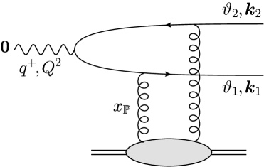
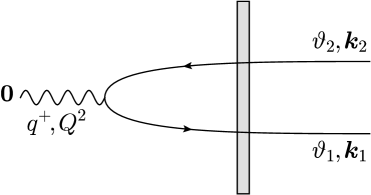
Figure 1: Exclusive dijet production in DIS off a nucleus, as described in the dipole picture. Left panel: one of the diagrams in the two-gluon exchange approximation. Right panel: the scattering off the nucleus is represented by a shockwave. It implicitly contains all diagrams with an arbitrary number of gluon exchanges, which can be hooked to the projectile system in all possible ways. In the present work it is assumed that the overall exchange, independently of its complexity, is always colourless.

The contribution of this process to the total diffractive cross section is obtained after integrating over the kinematics of the two jets for a fixed value of the rapidity gap $Y_{\mathbb{P}}$. Within collinear factorisation, this is conveniently written as

$$\frac{{\rm d}\sigma_{D}^{\gamma A\rightarrow XA}}{{\rm d}Y_{\mathbb{P}}}=\frac{4\pi^{2}\alpha_{em}}{Q^{2}}\,x_{\mathbb{P}}F_{2}^{D(3)}(x_{\rm\scriptscriptstyle Bj},x_{\mathbb{P}},Q^{2})\,,$$ (2)

where $X$ represents the “diffractive system” (for exclusive dijets, $X=q\bar{q}$), the factor $(4\pi^{2}\alpha_{em})/{Q^{2}}$ is the cross-section for photon absorption by a point-like particle with unit electric charge, and $F_{2}^{D(3)}$ is the diffractive structure function integrated over the momentum $t\equiv\Delta_{\perp}^{2}$ transferred by the target:

$$x_{\mathbb{P}}F_{2}^{D(3)}(x_{\rm\scriptscriptstyle Bj},x_{\mathbb{P}},Q^{2})\,\equiv\int{\rm d}t\,\frac{{\rm d}F_{2}^{D}}{{\rm d}Y_{\mathbb{P}}\,{\rm d}t}(x_{\rm\scriptscriptstyle Bj},x_{\mathbb{P}},Q^{2},t)\,.$$ (3)

In the leading twist (LT) approximation at large $Q^{2}$ — the main approximation underlying collinear factorisation — $F_{2}^{D(3)}$ is only weakly dependent upon $Q^{2}$ (via the DGLAP evolution) and can be expressed as a linear combination of diffractive parton distribution functions (DPDFs), with coefficient functions that can be computed within perturbative QCD. (These coefficient functions are the same as for inclusive DIS; see e.g. Golec-Biernat:2001gyl and references therein.) To leading order (LO) in pQCD, this combination involves the quark and antiquark DPDFs weighted by their electric charge squared and summed over the active flavours:

$$x_{\mathbb{P}}F_{2}^{D(3)}(x_{\rm\scriptscriptstyle Bj},x_{\mathbb{P}},Q^{2})=\sum_{f}e_{f}^{2}\big{[}\beta q^{D}_{f}(\beta,x_{\mathbb{P}},Q^{2})+\beta\bar{q}^{D}_{f}(\beta,x_{\mathbb{P}},Q^{2})\big{]}\qquad\mbox{(LT \& LO)}.$$ (4)

The diffractive DPDFs can be interpreted as the number of partons inside the Pomeron. And indeed, the quark and antiquark DPDFs appearing in the r.h.s. of Eq. (4) are expressed in terms of the longitudinal momentum fraction $\beta$ of the measured (anti)quark with respect to the Pomeron.

Within collinear factorisation, the diffractive PDFs are treated as non-perturbative quantities, that can be parameterised and fitted from the data. Within the dipole picture on the other hand, they can be explicitly computed, via mostly perturbative calculations Wusthoff:1997fz ; GolecBiernat:1999qd ; Hebecker:1997gp ; Buchmuller:1998jv ; Hautmann:1998xn ; Hautmann:1999ui ; Hautmann:2000pw ; Golec-Biernat:2001gyl . For instance, the leading order contribution to $F_{2}^{D(3)}$, hence to the quark DPDF, emerges from the dipole picture calculation of exclusive dijet production (see below).

Our main purpose in what follows is to demonstrate that results similar to (2)–(4) can be derived within the dipole picture already before (fully) integrating over the kinematics of the final state. In particular, for the $q\bar{q}$ final state to be discussed in this section, we shall show that one can write an “unintegrated” version of Eqs. (2)–(4), in which the (common) transverse momentum $\bm{K}$ of the two final jets is measured as well:

$$\frac{{\rm d}\sigma_{D}^{\gamma A\rightarrow q\bar{q}A}}{{\rm d}\ln(1/\beta)\,{\rm d}^{2}\bm{K}}=\frac{4\pi^{2}\alpha_{em}}{Q^{2}}\ 2\sum_{f}e_{f}^{2}\,\frac{{\rm d}\,\beta q^{D}_{f}(\beta,x_{\mathbb{P}},K_{\perp}^{2})}{{\rm d}^{2}\bm{K}}\,\qquad\mbox{(LT \& LO)}.$$ (5)

Such a process, in which one measures a single jet (or hadron) in the final state of DIS diffraction, is known as diffractive SIDIS (semi-inclusive deep inelastic scattering). For the leading-order process at hand, where the final quarks have equal but opposite transverse momenta, the difference between dijet production and SIDIS is rather trivial: it amounts to a $\delta$-function $\delta^{(2)}(\bm{k}_{1}+\bm{k}_{2})$ that has been integrated over in obtaining Eq. (5). The second factor in the r.h.s. of this equation plays the role of a quark diffractive TMD (transverse-momentum dependent distribution function). Our subsequent derivation of Eq. (5) from the dipole picture will support its interpretation as the unintegrated quark distribution of the Pomeron (see the right panel in Fig. 3 for a pictorial interpretation). As compared to Eq. (4), in (5) we have included just the quark DTMD and multiplied the result by a factor of two. Indeed, either the quark, or the antiquark, can be measured in the final state, and the respective contributions are identical, since the Pomeron is invariant under charge conjugation.

Unlike the more familiar relations (2)–(4) between the diffractive cross-section and the quark DPDF, its “unintegrated” version in (5) has never been discussed to our knowledge in the context of collinear factorisation. Yet, results which are suggestive of (5) have emerged in early discussions of DIS diffraction in the dipole picture Wusthoff:1997fz ; GolecBiernat:1999qd ; Hebecker:1997gp ; Buchmuller:1998jv ; Hautmann:1998xn ; Hautmann:1999ui ; Hautmann:2000pw ; Golec-Biernat:2001gyl , although the connection to TMD factorisation has not been mentioned at that time. Very recently, this connection has been established in Ref. Hatta:2022lzj (see especially Appendix B there), which is closer in spirit to our present approach.

As we shall see, the leading-twist approximation to diffraction is quite subtle, in that it includes a whole series of (formally, power-suppressed) corrections associated with multiple scattering and which are often referred to in the literature as “higher twist effects”. To avoid any confusion on this point, it is important to distinguish between two types of higher-twist corrections, which appear when computing diffraction within the dipole picture: the genuine “DIS twists”, which are proportional to powers of $K_{\perp}^{2}/Q^{2}$, and the “saturation twists”, which scale like powers of $Q_{s}^{2}/K_{\perp}^{2}$. The standard “leading-twist approximation” of the collinear factorisation is the lowest order term in the series of DIS twists, so its validity requires $K_{\perp}^{2}\ll Q^{2}$. Physically, it describes a situation where the virtual photon is absorbed by a single quark in the target wavefunction. Yet, this truncation of the DIS twists series imposes no constraint on the saturation twists, which describe multiple scattering between the $q\bar{q}$ dipole and the target gluon distribution. As we shall see, the leading-twist contribution to diffractive SIDIS includes “saturation twists” to all orders and is even dominated by strong scattering. In more physical terms, it is controlled by the physics of gluon saturation.

2.2 The cross-section for exclusive dijets

To compute diffraction in the colour dipole picture, we shall employ the light-cone wavefunction (LCWF) formalism, where the particles produced in the final state start as partonic fluctuations of the virtual photon: these fluctuations develop already long before the collision and are eventually put on-shell by their scattering with the nuclear target. This formalism is developed in the dipole frame, where the virtual photon (the “projectile”) and its partonic fluctuations are relativistic right movers, and in the projectile light-cone gauge $A^{+}=0$. This particular gauge choice is beneficial for at least two reasons: it permits a partonic (Fock–state) description for the wavefunction of the projectile and it allows for the eikonal coupling between the partons in the projectile and the “large” component $A^{-}_{a}$ of the colour field generated by the left-moving target. We are using the CGC description for the target wavefunction, in which the information about the gluon distribution is encoded in the correlations of the classical, random, fields $A^{-}_{a}$ Iancu:2002xk ; Iancu:2003xm ; Gelis:2010nm ; Kovchegov:2012mbw .

The general strategy for obtaining dijet cross sections in the CGC framework is well-known, see e.g. Dominguez:2011wm for a variety of processes computed at leading order. For definiteness, we shall follow the approach in Iancu:2022gpw , which considers both dijet and trijet production in DIS off a large nucleus. This approach has been originally developed for inclusive production, but its extension to diffractive processes is straightforward (see also Iancu:2021rup ; Iancu:2022lcw ; Beuf:2022kyp for related work). Our discussion will be rather succinct: we will merely sketch the crucial steps and the relevant results, while deferring the details to the literature.

In this section, we consider exclusive dijet production, so we focus on the $q\bar{q}$ component of the LCWF of the virtual photon, as depicted in Fig. 2. We take the quarks to be massless, so in practice we limit ourselves to the 3 light flavours $u,\,d,$ and $s$ (the sum over flavours will often be implicit in what follows). We present explicit calculations for the case of a virtual photon with transverse polarisation, but we shall later add the corresponding results for a longitudinal photon.

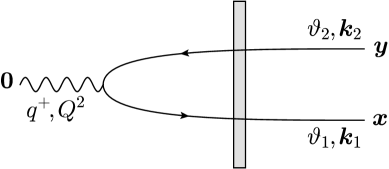
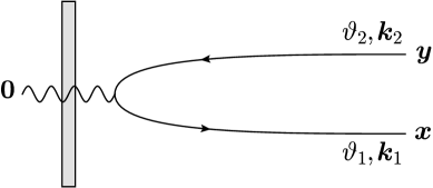
Figure 2: The probability amplitude for forward dijet production in DIS off a nuclear shockwave. Left panel: The $q\bar{q}$ pair interacts with the nucleus. Right panel: The no-scattering limit.

The general strategy can be summarised as follows Iancu:2018hwa ; Iancu:2020mos ; Iancu:2022gpw . We first compute the $q\bar{q}$ component in the absence of scattering and in momentum space, by using the Feynman rules of the light-cone perturbation theory (see e.g. Beuf:2016wdz ; Beuf:2017bpd ; Iancu:2018hwa ). Then we make a Fourier transform to the transverse coordinate representation and introduce the effects of the collision. The coordinate representation is better suited for that purpose since the transverse coordinates of the partons from the projectile are not modified by their high-energy scattering in the eikonal approximation. Finally, we return to momentum space, in order to specify the (longitudinal and transverse) momenta of the final quark and antiquark, assumed to be on-shell.

The $q\bar{q}$ component of the LCWF reads (in momentum space and in the absence of any collision)

$$\big{|}\gamma_{\scriptscriptstyle T}^{i}\big{\rangle}_{q\bar{q}}=\,\delta_{\alpha\beta}\int_{0}^{1} {\rm d}\vartheta_{1}{\rm d}\vartheta_{2}\,\delta(1-\vartheta_{1}-\vartheta_{2})\int{\rm d}^{2}\bm{k}_{1}{\rm d}^{2}\bm{k}_{2}\,\delta^{(2)}(\bm{k}_{1}+\bm{k}_{2})$$

$$\times\psi^{i}_{\lambda_{1}\lambda_{2}}(\vartheta_{1},\bm{k}_{1})\,\big{|}{q}_{\lambda_{1}}^{\alpha}(\vartheta_{1},\bm{k}_{1})\,\bar{q}_{\lambda_{2}}^{\beta}(\vartheta_{2},\bm{k}_{2})\big{\rangle},$$ (6)

with $i=1,2$ characterizing the photon polarization and $\alpha,\beta$ being color indices in the fundamental representation. $\lambda_{1}$, $\bm{k}_{1}$ and $\vartheta_{1}\equiv k_{1}^{+}/q^{+}$ are the helicity, transverse momentum and longitudinal fraction (w.r.t. the virtual photon) of the quark, and likewise for the antiquark. It is understood that there is a summation over the repeated indices $\alpha,\beta$ and $\lambda_{1},\lambda_{2}$. The $\delta$–function in colour space, $\delta_{\alpha\beta}$, shows that the $q\bar{q}$ pair forms a colour dipole. The $q\bar{q}$ amplitude appearing in Eq. (2.2) is given by

$$\psi^{i}_{\lambda_{1}\lambda_{2}}(\vartheta_{1},\bm{k}_{1})=\frac{\delta_{\lambda_{1}\lambda_{2}}}{2\sqrt{{2q^{+}}}}\frac{ee_{f}}{(2\pi)^{3}}\,\frac{1}{\vartheta_{1}(1-\vartheta_{1})}\,\frac{\varphi^{ij}(\vartheta_{1},\lambda_{1})\,k_{1}^{j}}{E_{q}+E_{\bar{q}}-E_{\gamma}},$$ (7)

where $e$ is the QED coupling, $e_{f}$ the fractional electric charge of the quark with flavor $f$. The function

$$\varphi^{ij}(\vartheta,\lambda)\equiv(2\vartheta-1)\delta^{ij}+2i\lambda\varepsilon^{ij}$$ (8)

with $\varepsilon^{ij}$ the Levi-Civita symbol in two dimensions, encodes the helicity structure of the photon splitting vertex, which is also proportional to the relative transverse velocity of the two fermions, namely (omitting an overall factor $1/q^{+}$)

$$\frac{\bm{k}_{1}}{\vartheta_{1}}-\frac{-\bm{k}_{1}}{1-\vartheta_{1}}=\frac{\bm{k}_{1}}{\vartheta_{1}(1-\vartheta_{1})}.$$ (9)

The light-cone (LC) energies and their combination appearing in the denominator read

$$E_{q}=\frac{k_{1\perp}^{2}}{2\vartheta_{1}q^{+}},\quad E_{\bar{q}}=\frac{k_{1\perp}^{2}}{2(1-\vartheta_{1})q^{+}},\quad E_{\gamma}=-\frac{Q^{2}}{2q^{+}},\quad E_{q}+E_{\bar{q}}-E_{\gamma}=\frac{k_{1\perp}^{2}+\bar{Q}^{2}}{2\vartheta_{1}(1-\vartheta_{1})q^{+}},$$ (10)

where we have defined $\bar{Q}^{2}\equiv\vartheta_{1}(1-\vartheta_{1})Q^{2}$. Substituting the above energy denominator into Eq. (7) we trivially find

$$\psi^{i}_{\lambda_{1}\lambda_{2}}(\vartheta_{1},\bm{k}_{1})=\delta_{\lambda_{1}\lambda_{2}}\,\sqrt{\frac{q^{+}}{2}}\,\frac{ee_{f}}{(2\pi)^{3}}\,\frac{\varphi^{ij}(\vartheta_{1},\lambda_{1})\,k_{1}^{j}}{k_{1\perp}^{2}+\bar{Q}^{2}}.$$ (11)

This probability amplitude can be transformed to coordinate space via the replacement

$$\frac{k_{1}^{j}}{k_{1\perp}^{2}+\bar{Q}^{2}}\to\int\frac{{\rm d}^{2}\bm{k}_{1}}{(2\pi)^{2}}\,e^{i\bm{k}_{1}\cdot\bm{R}}\,\frac{k_{1}^{j}}{k_{1\perp}^{2}+\bar{Q}^{2}}=\frac{i}{2\pi}\,\frac{R^{j}}{R}\,\bar{Q}K_{1}(\bar{Q}R),$$ (12)

where $\bm{R}\equiv\bm{x}-\bm{y}$, with $\bm{x}$ and $\bm{y}$ the transverse coordinates of the quark and the antiquark respectively. The modified Bessel function $K_{1}$ vanishes exponentially for dipoles sizes $R\equiv|\bm{R}|$ much larger than $1/\bar{Q}$. This shows that the typical value for the dipole size is $R\sim 1/\bar{Q}$. Importantly, this depends not only upon the virtuality of the incoming photon, but also upon the longitudinal momentum sharing by the two fermions.

As already explained, the excursion through the coordinate space is useful for adding the effects of the interaction with the nuclear target (a Lorentz contracted shockwave): as a result of this interaction, each partonic component of the projectile acquires a colour rotation implemented by a suitable Wilson line. For the $q\bar{q}$ component, we can write

$$\hat{S}\big{|}{q}_{\lambda_{1}}^{\alpha}(\vartheta_{1},\bm{x})\,\bar{q}_{\lambda_{2}}^{\beta}(\vartheta_{2},\bm{y})\big{\rangle}\,=\,\left(V(\bm{x})\,V^{\dagger}(\bm{y})\right)_{\alpha\beta}\,\big{|}{q}_{\lambda_{1}}^{\alpha}(\vartheta_{1},\bm{x})\,\bar{q}_{\lambda_{2}}^{\beta}(\vartheta_{2},\bm{y})\big{\rangle}$$ (13)

where $V(\bm{x})$ (for the quark) and $V^{\dagger}(\bm{y})$ (for the antiquark) are Wilson lines in the fundamental representation of the colour group, e.g.

$$V(\bm{x})={\rm T}\exp\left[ig\int{\rm d}x^{+}t^{a}A^{-}_{a}(x^{+},\bm{x})\right],$$ (14)

where the symbol T stands for LC time ($x^{+}$) ordering. Hence, after changing to the coordinate representation and adding the effects of the collision, the colour structure of the LCWF (2.2) gets modified as follows:

$$\delta_{\alpha\beta}\rightarrow\big{[}V(\bm{x})V^{\dagger}(\bm{y})-\mathds{1}\big{]}_{\alpha\beta},$$ (15)

where we have also subtracted the no-scattering limit, which corresponds to the diagram shown in the right panel of Fig. 2. More precisely, the replacement in Eq. (15) leads to the inclusive production of a dijet. In order to have a diffractive process to the order of accuracy, we must ensure that the colour dipole scatter elastically off the nuclear target, i.e. it remains a colour singlet in the final state. This is achieved by the following projection

$$\big{[}V(\bm{x})V^{\dagger}(\bm{y})-\mathds{1}\big{]}_{\alpha\beta}\rightarrow\left\{\frac{1}{N_{c}}\,{\rm tr}\big{[}V(\bm{x})V^{\dagger}(\bm{y})\big{]}-1\right\}\delta_{\alpha\beta}\equiv[S(\bm{x},\bm{y})-1]\,\delta_{\alpha\beta}\equiv-T(\bm{x},\bm{y})\,\delta_{\alpha\beta},$$ (16)

where $S(\bm{x},\bm{y})$ is the dipole $S$-matrix for elastic scattering and $T(\bm{x},\bm{y})$ is the corresponding $T$-matrix.

When calculating the cross section, one encounters the product $T(\bm{x},\bm{y})T(\bar{\bm{y}},\bar{\bm{x}})$, with $(\bar{\bm{x}},\bar{\bm{y}})$ the dipole coordinates in the complex conjugate amplitude (CCA). In the CGC framework this product must be averaged over all possible target field configurations, with a weight function which takes into account the BK/JIMWLK evolution Balitsky:1995ub ; Kovchegov:1999yj ; JalilianMarian:1997jx ; JalilianMarian:1997gr ; Kovner:2000pt ; Weigert:2000gi ; Iancu:2000hn ; Iancu:2001ad ; Ferreiro:2001qy of the gluon distribution up to the rapidity scale of interest (see below). Still for the purpose of the elastic scattering, one must keep only the factorised piece in the average of the product, that is

$$\left\langle T(\bm{x},\bm{y})T(\bar{\bm{y}},\bar{\bm{x}})\right\rangle\to\left\langle T(\bm{x},\bm{y})\right\rangle\left\langle T(\bar{\bm{y}},\bar{\bm{x}})\right\rangle.$$ (17)

Indeed, the colour flow on the target side must close separately in the direct ampltiude (DA) and in the CCA, as a necessary condition to have a coherent process. For simplicity, we will also assume that the nucleus is homogeneous and therefore any target average can depend only on the differences between the various transverse coordinates. Thus, the average dipole scattering amplitude takes the form $\left\langle T(\bm{x},\bm{y})\right\rangle=\mathcal{T}(\bm{R})$, with $\bm{R}=\bm{x}-\bm{y}$. (Note that we shall systematically use calligraphic notations for the averaged quantities.) All in all, when calculating coherent diffraction with a homogeneous nucleus, the eikonal scattering is taken into account by simply letting

$$\delta_{\alpha\beta}\to-\mathcal{T}(\bm{R})\,\delta_{\alpha\beta},$$ (18)

within the coordinate-space version of the LCWF for the $q\bar{q}$ component. After this step, Eq. (12) gets replaced by

$$\frac{i}{2\pi}\,\frac{R^{j}}{R}\,\bar{Q}K_{1}(\bar{Q}R) \to-\frac{i}{2\pi}\,\frac{R^{j}}{R}\,\bar{Q}K_{1}(\bar{Q}R)\mathcal{T}(\bm{R})\to-\frac{i}{2\pi}\int{\rm d}^{2}\bm{R}\,e^{-i\bm{k}_{1}\cdot\bm{R}}\,\frac{R^{j}}{R}\,\bar{Q}K_{1}(\bar{Q}R)\mathcal{T}(\bm{R})$$

$$=-\frac{k_{1}^{j}}{k_{1\perp}}\int{\rm d}R\,R\,J_{1}(k_{1\perp}R)\,\bar{Q}K_{1}(\bar{Q}R)\,\mathcal{T}(R),$$ (19)

where we have also performed the inverse Fourier transform to transverse momentum space and, in doing that, we assumed target isotropy, for simplicity: $\mathcal{T}(\bm{R})=\mathcal{T}(R)$.

To summarise, the generalisation of the probability amplitude in Eq. (11) which includes the effects of the collision with the nuclear target reads as follows

$$\psi^{i,D}_{\lambda_{1}\lambda_{2}}(\vartheta_{1},\bm{k}_{1})=-\delta_{\lambda_{1}\lambda_{2}}\,\sqrt{\frac{q^{+}}{2}}\,\frac{ee_{f}}{(2\pi)^{3}}\,\varphi^{ij}(\vartheta_{1},\lambda_{1})\,\frac{k_{1}^{j}}{k_{1\perp}}\,\frac{\mathcal{Q}_{T}(\bar{Q},k_{1\perp})}{\bar{Q}},$$ (20)

where we have introduced the dimensionless, scalar function

$$\mathcal{Q}_{T}(\bar{Q},K_{\perp},Y_{\mathbb{P}})\equiv\bar{Q}^{2}\int{\rm d}R\,R\,J_{1}(K_{\perp}R)\,K_{1}(\bar{Q}R)\,\mathcal{T}(R,Y_{\mathbb{P}}).$$ (21)

Strictly speaking, the momentum $\bm{k}_{1}$ of the quark after the scattering, as appearing in Eq. (20), is different from the one before the scattering in Eq. (11), even though we have used the same notation. But it is important to notice that the $\delta$–function imposing $\bm{k}_{1}+\bm{k}_{2}=0$ still holds, like in Eq. (2.2). This is due to the elastic nature of the scattering (which enforced the factorisation of the average scattering amplitude, cf. Eq. (17)) and also to the assumed homogeneity of the target (which is tantamount to our original assumption that $\Delta_{\perp}\sim 1/R_{A}\sim\ 30$ MeV is truly negligible compared to $k_{1\perp}$ and $k_{2\perp}$).

The cross section for exclusive dijet production is finally determined by calculating the number of quarks and antiquarks in the final state with the desired longitudinal and transverse momenta. For the precise normalization of the respective number operators, as well as of the states appearing in Eq. (2.2), we follow Iancu:2018hwa to obtain

$$\frac{{\rm d}\sigma^{\gamma_{\scriptscriptstyle T}^{*}A\rightarrow q\bar{q}A}}{{\rm d}\vartheta_{1}{\rm d}\vartheta_{2}\,{\rm d}^{2}\bm{k}_{1}{\rm d}^{2}\bm{k}_{2}}=\frac{(2\pi)^{3}S_{\perp}N_{c}}{2q^{+}}\,\delta(1-\vartheta_{1}-\vartheta_{2})\,\delta^{(2)}(\bm{k}_{1}+\bm{k}_{2})\sum_{i,\lambda_{1},\lambda_{2}}\big{|}\psi_{\lambda_{1}\lambda_{2}}^{i,D}\big{|}^{2},$$ (22)

where $S_{\perp}$ is the transverse are of the nucleus. The above is of course proportional to the square of the probability amplitude in Eq. (20) which is easily calculated. By further doing the trivial integration over the antiquark using the $\delta$-functions and summing over the photon transverse polarisations, over the quark helicities, and over all active flavors, we arrive at

$$\frac{{\rm d}\sigma^{\gamma_{\scriptscriptstyle T}^{*}A\rightarrow q\bar{q}A}}{{\rm d}\vartheta_{1}\,{\rm d}^{2}\bm{K}}=\frac{S_{\perp}\alpha_{\rm em}N_{c}}{2\pi^{2}}\left(\sum e_{f}^{2}\right)\left[\vartheta_{1}^{2}+(1-\vartheta_{1})^{2}\right]\frac{[\mathcal{Q}_{T}(\bar{Q},K_{\perp},Y_{\mathbb{P}})]^{2}}{\bar{Q}^{2}},$$ (23)

where $\alpha_{\rm em}=e^{2}/4\pi$ and we defined $\bm{K}\equiv-\bm{k}_{1}=\bm{k}_{2}$ for convenience. The $\gamma\to q\bar{q}$ splitting function visible in the r.h.s. has been generated via the identity:

$$\varphi^{ij}(\vartheta,\lambda)\,\varphi^{il\,*}(\vartheta,\lambda)\,=\,2\delta^{jl}\left[\vartheta^{2}+(1-\vartheta)^{2}\right].$$ (24)

As indicated by our above notations, see e.g. Eq. (21), the quantity $\mathcal{Q}_{T}$ also depends upon $Y_{\mathbb{P}}$, via the corresponding dependence of the dipole amplitude $\mathcal{T}(R,Y_{\mathbb{P}})$. We recall that $Y_{\mathbb{P}}$ is the rapidity separation between the diffractive system (here, the $q\bar{q}$ pair) and the target. Importantly, this refers to target rapidity, i.e. to the fraction $x_{\mathbb{P}}$ of the longitudinal momentum $P_{N}^{-}$ of a nucleon from the target which is transferred to the diffractive system via the collision. We more precisely have $Y_{\mathbb{P}}=\ln 1/x_{\mathbb{P}}$, where the value of $x_{\mathbb{P}}$ is fixed by the condition that the final $q\bar{q}$ pair be on-shell:

$$x_{\mathbb{P}}P_{N}^{-}=\frac{1}{2q^{+}}\left(\frac{k_{1\perp}^{2}}{\vartheta_{1}}+\frac{k_{2\perp}^{2}}{\vartheta_{2}}+Q^{2}\right)\,\Longrightarrow\,x_{\mathbb{P}}=\frac{1}{\hat{s}}\left[Q^{2}+\frac{K_{\perp}^{2}}{\vartheta_{1}(1-\vartheta_{1})}\right],$$ (25)

with $\hat{s}=2q^{+}P_{N}^{-}$. This has the structure anticipated in Eq. (1), with the expected value for the diffractive mass of the $q\bar{q}$ final state, that is, $M_{X}^{2}={K_{\perp}^{2}}/\vartheta_{1}\vartheta_{2}$. For this particular process, the diffractive variable $\beta$ introduced too in Eq. (1) takes the form:

$$\beta\equiv\frac{x_{\rm\scriptscriptstyle Bj}}{x_{\mathbb{P}}}=\frac{\bar{Q}^{2}}{\bar{Q}^{2}+K_{\perp}^{2}}.$$ (26)

2.3 Diffractive SIDIS and its leading-twist approximation

In this section, we shall use Eq. (23) to construct the cross-section (5) for diffractive SIDIS and then we shall isolate its leading-twist contribution and eventually recover the factorised structure anticipated in the r.h.s. of Eq. (5).

Clearly, in order to go from Eq. (23) to Eq. (5) one just needs to perform a change of longitudinal variables, from $\vartheta_{1}$ to $\beta$, which can be easily done with the help of (26). Although mathematically trivial, this change of variables is truly important if one is interested in building a physical interpretation for this process in terms of the evolution of the target. Indeed, $\beta$ represents the longitudinal momentum fraction w.r.t. the Pomeron of the quark from the target that is struck by the virtual photon. This interpretation implicitly assumes that the photon was absorbed by a single quark, which is indeed the case in the leading-twist (LT) approximation. In this analysis, we shall discover that the LT contribution to the cross-section corresponds to aligned jet configurations in the dipole picture: $\vartheta_{1}(1-\vartheta_{1})\ll 1$. This is important too for building a target picture: in order for a parton (here, one of the two final quarks) to be transferred from the wavefunction of the projectile to that of the target, that parton must have a negligible longitudinal momentum along the direction of motion of the projectile.

One can perform the aforementioned change of variables by integrating over $\vartheta_{1}$ with a $\delta$–function enforcing the condition (26):

$$\frac{{\rm d}\sigma^{\gamma_{T}^{*}A\rightarrow q\bar{q}A}}{{\rm d}\ln(1/\beta)\,{\rm d}^{2}\bm{K}}=\int_{0}^{1}{\rm d}\vartheta_{1}\,\beta\delta\left(\beta-\frac{\bar{Q}^{2}}{\bar{Q}^{2}+K_{\perp}^{2}}\right)\frac{{\rm d}\sigma^{\gamma_{\scriptscriptstyle T}^{*}A\rightarrow q\bar{q}A}}{{\rm d}\vartheta_{1}\,{\rm d}^{2}\bm{K}}\,.$$ (27)

The $\delta$–function is conveniently rewritten as (recall that $\bar{Q}^{2}=\vartheta_{1}(1-\vartheta_{1})Q^{2}$)

$$\beta\delta\left(\beta-\frac{\bar{Q}^{2}}{\bar{Q}^{2}+K_{\perp}^{2}}\right) \,=\frac{\vartheta_{1}(1-\vartheta_{1})}{1-\beta}\,\delta\left(\vartheta_{1}(1-\vartheta_{1})-\frac{\beta}{1-\beta}\frac{K_{\perp}^{2}}{Q^{2}}\right)$$ (28)

$$\,=\,\frac{\vartheta_{1}(1-\vartheta_{1})}{1-\beta}\,\frac{\delta\left(\vartheta_{1}-\vartheta_{*}\right)+\delta\left(\vartheta_{1}-1+\vartheta_{*}\right)}{1-2\vartheta_{*}}\ \longrightarrow\ \frac{2\vartheta_{*}(1-\vartheta_{*})}{(1-2\vartheta_{*})(1-\beta)}\,\delta\left(\vartheta_{1}-\vartheta_{*}\right).$$

Here $\vartheta_{*}$ and $1-\vartheta_{*}$ are the two values of $\vartheta_{1}$ selected by the $\delta$–function and we conveniently chose $\vartheta_{*}$ to be smaller than 1/2:

$$\vartheta_{*}\,=\,\frac{1}{2}\left(1-\sqrt{1-\frac{4\beta}{1-\beta}\frac{K_{\perp}^{2}}{Q^{2}}}\right)\qquad\mbox{with}\quad K_{\perp}^{2}\,\leq\,\frac{1-\beta}{4\beta}\,Q^{2}\,.$$ (29)

The integrand in Eq. (27) is symmetric under the exchange $\vartheta_{1}\to 1-\vartheta_{1}$, hence it is sufficient to keep this smaller solution $\vartheta_{*}$ and multiply the result by 2, as indicated in the second line of Eq. (28). In terms of these new variables $K_{\perp}$ and $\beta$, the value of $\bar{Q}$ is computed as

$$\bar{Q}^{2}\,=\,\frac{\beta}{1-\beta}\,K_{\perp}^{2}\equiv\mathcal{M}^{2},$$ (30)

hence it is independent of $Q^{2}$. A simple calculation yields

$$\frac{{\rm d}\sigma^{\gamma_{T}^{*}A\rightarrow q\bar{q}A}}{{\rm d}\ln(1/\beta)\,{\rm d}^{2}\bm{K}}=\frac{S_{\perp}\alpha_{\rm em}N_{c}}{\pi^{2}}\left(\sum e_{f}^{2}\right)\,\frac{1}{Q^{2}}\,\frac{1-\frac{2\mathcal{M}^{2}}{Q^{2}}}{\sqrt{1-\frac{4\mathcal{M}^{2}}{Q^{2}}}}\,\frac{[\mathcal{Q}_{T}(\mathcal{M},K_{\perp},Y_{\mathbb{P}})]^{2}}{1-\beta}\,.$$ (31)

When $\mathcal{M}^{2}\ll Q^{2}$, one can expand the expression under the square root, thus generating the twist-expansion of Eq. (31): an infinite series of power corrections which scale like powers of $\mathcal{M}^{2}/Q^{2}$. For generic values of $\beta$, which are not very small, nor very close to one, one has $\mathcal{M}^{2}\sim K_{\perp}^{2}$, so these corrections can be recognised as the “DIS higher-twists” discussed at the end of Sect. 2.1. To make contact with Eq. (5), we need to isolate the leading-twist piece in this series, that is, the dominant contribution in the limit $Q^{2}\gg\mathcal{M}^{2}$. (The relevance of this limit for the physical problem at hand will be clarified in the next sections.) One easily finds

$$\frac{{\rm d}\sigma^{\gamma_{T}^{*}A\rightarrow q\bar{q}A}}{{\rm d}\ln(1/\beta)\,{\rm d}^{2}\bm{K}}=\frac{S_{\perp}\alpha_{\rm em}N_{c}}{\pi^{2}}\left(\sum e_{f}^{2}\right)\,\frac{1}{Q^{2}}\,\frac{[\mathcal{Q}_{T}(\mathcal{M},K_{\perp},Y_{\mathbb{P}})]^{2}}{1-\beta}\,\quad\mbox{when}\quad Q^{2}\gg\mathcal{M}^{2}\,.$$ (32)

As anticipated, this result has the factorised structure anticipated in Eq. (5). The whole $Q^{2}$–dependence is now isolated in the overall power-law $1/Q^{2}$, which is the hallmark of the elementary cross-section for photon absorption by a point-like quark form the target.

Recalling Eq. (29), one sees that the condition $\mathcal{M}^{2}/Q^{2}\ll 1$ for the validity of Eq. (32) automatically selects the asymmetric $q\bar{q}$ pairs with $\vartheta_{*}\simeq\mathcal{M}^{2}/Q^{2}\ll 1$. This strong correlation between the LT approximation and the aligned jet configurations can be understood as follows: when $\vartheta_{*}\ll 1$, one of the two fermions of the dipole picture — that with longitudinal fraction $1-\vartheta_{*}\simeq 1$ — carries most of the longitudinal momentum $q^{+}$ of the incoming photon and hence can be unambiguously identified as the quark from the target that has absorbed the photon.

This simple analysis illustrates some of the main steps that we shall encounter in more complicated situations, in the process of shifting from the colour dipole picture to the target picture: a change in longitudinal variables (from projectile-oriented to target-oriented longitudinal momentum fractions), the leading-twist approximation at high $Q^{2}$ (or for large jet transverse momenta), and the focus on asymmetric configurations. In practice, the last two steps often come together: when working in the target-oriented variables, the restriction to asymmetric dijets automatically implements the relevant LT approximation.

2.4 TMD factorisation for diffractive SIDIS

The leading-twist approximation (32) to the cross-section for diffractive SIDIS exhibits a factorised form, which is consistent with TMD factorisation. Specifically,

$$\frac{{\rm d}\sigma^{\gamma_{T}^{*}A\rightarrow q\bar{q}A}}{{\rm d}\ln(1/\beta)\,{\rm d}^{2}\bm{K}}=\frac{4\pi^{2}\alpha_{em}}{Q^{2}}\big{(}\sum e_{f}^{2}\big{)}\,2\,\frac{{\rm d}xq_{\mathbb{P}}(x,x_{\mathbb{P}},K_{\perp}^{2})}{{\rm d}^{2}\bm{K}}\bigg{|}_{x=\beta}.$$ (33)

with the following expression for the quark (or antiquark) diffractive TMD:

$$\frac{{\rm d}xq_{\mathbb{P}}(x,x_{\mathbb{P}},K_{\perp}^{2})}{{\rm d}^{2}\bm{K}}\equiv\frac{S_{\perp}N_{c}}{4\pi^{3}}\,\frac{[\mathcal{Q}_{\mathbb{P}}(x,x_{\mathbb{P}},K_{\perp}^{2})]^{2}}{2\pi(1-x)}\,\equiv\,S_{\perp}\,\frac{2N_{c}}{(2\pi)^{3}}\,\Psi_{\mathbb{P}}(x,x_{\mathbb{P}},K_{\perp}^{2})\,,$$ (34)

where $x$ is the longitudinal momentum fraction of the measured (anti)quark w.r.t. the Pomeron and $\mathcal{Q}_{\mathbb{P}}(x,x_{\mathbb{P}},K_{\perp}^{2})$ is the same as the quantity $\mathcal{Q}_{T}(\bar{Q},K_{\perp},Y_{\mathbb{P}})$ previously introduced in Eq. (21), but which is now viewed as a function of only target kinematical variables, like the TMD:

$$\mathcal{Q}_{\mathbb{P}}(x,x_{\mathbb{P}},K_{\perp}^{2})\equiv\mathcal{M}^{2}\int_{0}^{\infty}{\rm d}R\,R\,J_{1}(K_{\perp}R)\,K_{1}(\mathcal{M}R)\,\mathcal{T}(R,Y_{\mathbb{P}})$$ (35)

It is understood that $\mathcal{M}^{2}=\frac{x}{1-x}K_{\perp}^{2}$ (cf. Eq. (30) with $\beta\to x$). The interpretation of the quantity $\Psi_{\mathbb{P}}(x,x_{\mathbb{P}},K_{\perp}^{2})$ will be shortly explained.

In what follows, we would like to argue that this quark TMD can naturally be interpreted as the unintegrated quark distribution of the Pomeron — that is, the number of quarks (or antiquarks) of a given flavour that can be found in the light-cone wavefunction of the Pomeron with longitudinal momentum fraction $x$ and with transverse momentum $\bm{K}$:

$$\frac{{\rm d}xq_{\mathbb{P}}(x,x_{\mathbb{P}},K_{\perp}^{2})}{{\rm d}^{2}\bm{K}}\,=\,x\,\frac{{\rm d}N_{q\in\mathbb{P}}}{{\rm d}x{\rm d}^{2}\bm{K}}\,.$$ (36)

With this interpretation, the quantity $\Psi_{\mathbb{P}}(x,x_{\mathbb{P}},K_{\perp}^{2})$ introduced in the last equality Eq. (34) has the meaning of the quark occupation number.

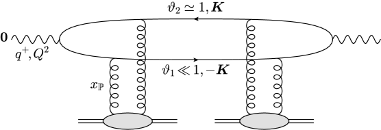
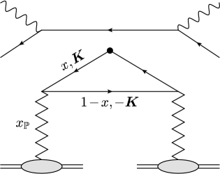
Figure 3: Cross section for the exclusive dijet production with a soft quark in DIS off a nucleus. Left panel: the viewpoint of the colour dipole picture. Right panel: the pictorial illustration of TMD factorisation. The soft quark, with longitudinal fraction $1-x$, is now radiated from the Pomeron and thus belongs to the target wavefunction. The virtual photon probes the (anti)quark DTMD evaluated at fraction $x$ and transverse momentum $\bm{K}$.

This partonic interpretation of the quark DTMD could be unambiguously established only by working in the target infinite momentum (or Bjorken) frame and in the target light-cone gauge $A^{-}=0$: indeed, these are the frame and gauge where the construction of the light-cone wavefunction makes sense for a relativistic left-mover. That said, the cross-section is boost and gauge invariant, hence the partonic interpretation can also be a posteriori recognised when working in the dipole picture, provided one focuses on the leading-twist approximation at large $Q^{2}\gg Q_{s}^{2}(Y_{\mathbb{P}})$ and one uses the target longitudinal momentum fraction $x$ instead of the projectile momentum fraction $\vartheta_{1}$.

Specifically, we would like to argue that Eq. (33) is consistent with the following physical picture in the Bjorken frame, as illustrated in the right panel in Fig. 3: the virtual photon, which in this new frame is relatively slow ($q^{+}\sim Q$), is absorbed by a quark-antiquark pair which represents the final evolution of a colourless partonic fluctuation of the target — the “Pomeron”. This Pomeron carries a tiny (net) transverse momentum $\Delta_{\perp}\sim 1/R_{A}$, which is negligible for our purposes, and a small fraction $x_{\mathbb{P}}\ll 1$ of the target longitudinal momentum $P_{N}^{-}$, that is transmitted to the $q\bar{q}$ pair. One of the fermions in this pair, say the quark with splitting fraction $1-x$ and transverse momentum $-\bm{K}$, is already on mass-shell and appears in the final state. This quark does not interact with the virtual photon, rather it plays the role of a spectator. The other fermion — a $t$–channel antiquark with splitting fraction $x$ and transverse momentum $\bm{K}$ — is virtual and scatters with the hard photon in order to produce the final, on-shell, antiquark. From the viewpoint of the color dipole picture, cf. the left panel in Fig. 3, the virtual antiquark is the intermediate quark in between the photon decay vertex and the scattering with the target. This fermion looks like a right-moving quark in the dipole frame, but like a left-moving antiquark after boosting to the Bjorken frame.

The spectator ($s$–channel) quark carries a fraction $(1-x)x_{\mathbb{P}}$ of the target momentum and a fraction $\vartheta_{1}$ of the longitudinal momentum $q^{+}$ of the virtual photon, hence the condition to be on-shell reads

$$2\vartheta_{1}(1-x)x_{\mathbb{P}}q^{+}P_{N}^{-}=K_{\perp}^{2}\,\Longrightarrow\,(1-x)x_{\mathbb{P}}=\frac{K_{\perp}^{2}}{\vartheta_{1}\hat{s}}.$$ (37)

The $t$–channel antiquark has $k^{+}=-\vartheta_{1}q^{+}$ and $k^{-}=xx_{\mathbb{P}}P_{N}^{-}$, hence a space-like virtuality

$$k^{2}=2k^{+}k^{-}-K_{\perp}^{2}=-\vartheta_{1}xx_{\mathbb{P}}\hat{s}-K_{\perp}^{2}=-\frac{K_{\perp}^{2}}{1-x}\,.$$ (38)

Taking the ratio of Eqs. (25) and (37) and solving either for $\bar{Q}$ or for $x$ we find

$$\bar{Q}^{2}=\frac{x-\vartheta_{1}}{1-x}\,K_{\perp}^{2}\,\Longleftrightarrow\,x=\frac{\bar{Q}^{2}+\vartheta_{1}K_{\perp}^{2}}{\bar{Q}^{2}+K_{\perp}^{2}}.$$ (39)

This equation shows that, in general, $\bar{Q}^{2}$ cannot be expressed uniquely in terms of the two variables $x$ and $K_{\perp}^{2}$ which characterise the production of the $q\bar{q}$ pair by the Pomeron — it also depends upon the projectile variable $\vartheta_{1}$. Moreover, $x$ is not the same as $\beta$ (compare the second equation above to Eq. (26)). Yet, when the spectator quark is soft w.r.t. the virtual photon, i.e. when $\vartheta_{1}\ll 1$, the first equation in (39) reduces to

$$\bar{Q}^{2}\simeq\vartheta_{1}Q^{2}\simeq\frac{x}{1-x}\,K_{\perp}^{2},$$ (40)

which is now a function of only $x$ and $K_{\perp}^{2}$, as required by factorisation. Still for $\vartheta_{1}\ll 1$, the second equation in (39) becomes

$$x\simeq\frac{\bar{Q}^{2}}{\bar{Q}^{2}+K_{\perp}^{2}}=\beta,$$ (41)

and then Eqs. (40) and (30) are indeed consistent with each other.

Clearly, if within the original expression (23) for the cross-section one makes a change of variables from $\vartheta_{1}$ to $x$ and one uses $\vartheta_{1}\ll 1$, together with (40) and (41), then one finds the leading-twist approximation in Eq. (32) with $\beta=x$. We thus recover the correlation between aligned jets and the LTA, as discussed at the end of Sect. 2.3. This correlation is easy to understand on the basis of Eq. (40) which shows that, for fixed and generic values of $x$, the variable $\vartheta_{1}$ scales like $\vartheta_{1}\sim K_{\perp}^{2}/Q^{2}$. Hence, by working at leading order in the small parameter $\vartheta_{1}$, one automatically selects the dominant contributions in the twist expansion at high $Q^{2}$.

To summarise, both the mathematical derivation of the TMD factorisation for diffractive SIDIS from the dipole picture, and its physical interpretation in terms of parton evolution in the target, crucially rely on the fact that the produced $q\bar{q}$ pair is very asymmetric: $\vartheta_{1}\vartheta_{2}\ll 1$. In the next subsection, we shall argue that this condition is very well satisfied for the typical diffractive processes — those which give the dominant contribution to $F_{2}^{D}$.

2.5 Multiple scattering and parton saturation in the Pomeron

In this section, we will study in some detail the quark DTMD defined in Eq. (34), with the purpose of demonstrating (via parametric estimates) two important features: (i) this distribution saturates at relatively low momenta, $K_{\perp}\lesssim Q_{s}$, but (ii) it abruptly falls, like the power $Q_{s}^{4}/K_{\perp}^{4}$, at much larger momenta. This shows that the typical quark-antiquark pairs produced by the Pomeron are semi-hard, i.e. they carry transverse momenta $K_{\perp}\sim Q_{s}$. (In Iancu:2021rup ; Iancu:2022lcw , similar conclusions have been reached for the gluon diffractive TMD.) These results can be translated to the original, dipole, picture with the help of the relation (40) between projectile and target variables: for $K_{\perp}\sim Q_{s}$ and generic values of $x$, this relation implies

$$\vartheta_{1}\simeq\frac{x}{1-x}\,\frac{K_{\perp}^{2}}{Q^{2}}\,\sim\,\frac{Q_{s}^{2}}{Q^{2}}\,\ll 1\,.$$ (42)

This shows that the $q\bar{q}$ fluctuations of the virtual photon which are predominantly produced via elastic scattering are very asymmetric, with a low effective virtuality $\bar{Q}^{2}\simeq\vartheta_{1}Q^{2}\sim Q_{s}^{2}$ and hence a large transverse size $R\sim 1/Q_{s}$. Such large colour dipoles undergo strong scattering, $\mathcal{T}(R)\sim 1$, and thus are strongly favoured by the elastic nature of the scattering, i.e. by the fact that the SIDIS cross-section is proportional to the square $\mathcal{T}^{2}$ of the dipole scattering amplitude.

These conclusions heavily rely on the interplay between the structure of the virtual photon LCWF and the scattering of the $q\bar{q}$ dipole. In the target viewpoint underlying the TMD factorisation (33), these two fundamental aspects are both encoded in the function $\mathcal{Q}_{\mathbb{P}}(x,x_{\mathbb{P}},K_{\perp}^{2})$ defined in Eq. (35). In particular, the quantity $\mathcal{M}^{2}=\frac{x}{1-x}\,K_{\perp}^{2}$ appearing in this equation is nothing but the effective virtuality $\bar{Q}^{2}$ of the dipole picture expressed in terms of target variables, cf. Eq. (40).

For the subsequent discussion, we also need an explicit form for the dipole scattering amplitude $\mathcal{T}(R)$, that we shall take from the McLerran-Venugopalan (MV) model McLerran:1993ni ; McLerran:1994vd . This model is meant to apply for a large nucleus ($A\gg 1$) at moderate energies ($x_{\mathbb{P}}\gtrsim 10^{-2}$) and provides a physically motivated initial condition for the high-energy (BK-JIMWLK) evolution with increasing $Y_{\mathbb{P}}$. It assumes that the dipole projectile scatters off a Gaussian colour charge distribution representing the valence quarks. One finds

$$\mathcal{T}(R)=1-\exp\left(-\frac{R^{2}Q_{A}^{2}}{4}\,\ln\frac{4}{R^{2}\Lambda^{2}}\right),$$ (43)

where $Q_{A}^{2}$ is essentially the density of the colour charge squared of the valence quarks in the transverse plane. By expanding the exponential in the r.h.s. one generates the multiple scattering series (the “saturation twists” alluded to at the end of Sect. 2.1). The first term in this expansion, which coincides with the exponent in Eq. (43), represents the amplitude for a single elastic scattering via two gluon exchange. For a sufficiently large dipole though, the scattering becomes strong (the exponent is of order one, or larger), and then one needs to include multiple scattering to all orders. The saturation momentum $Q_{s}$ is the scale which defines the onset of multiple scattering. It is conventionally defined as the value of $2/R$ for which the exponent becomes of order one:

$$Q_{s}^{2}=Q_{A}^{2}\ln\frac{Q_{s}^{2}}{\Lambda^{2}}\,.$$ (44)

We are now in a position to analyse the behaviour of Eq. (35) in various limits. The integral over $R$ in Eq. (35) is controlled by the interplay between three functions: the two Bessel functions $K_{1}(\mathcal{M}R)$ and $J_{1}(K_{\perp}R)$, and the dipole scattering amplitude $\mathcal{T}(R,Y_{\mathbb{P}})$. The Bessel functions are rapidly decreasing (or oscillating) for large values of their respective arguments, hence they restrict the maximal value of $R$. On the contrary, the dipole amplitude favours large dipole sizes $R\gtrsim 1/Q_{s}(Y_{\mathbb{P}})$, for which the scattering is as strong as possible.

For parametric estimates, it suffices to use a piecewise approximation to the dipole amplitude in Eq. (43) (more sophisticated approximations, which take into account the full structure of the MV model amplitude and also include its BK evolution with increasing $Y_{\mathbb{P}}$, will be considered in Sect. 6.1):

$$\mathcal{T}(R)\,\simeq\begin{cases}\displaystyle{\ R^{2}Q_{s}^{2}}&\text{for \ $R\!\ll 1/Q_{s}$,}\\[5.69046pt] \displaystyle{\ 1}&\text{for \ $R\!\gtrsim 1/Q_{s}$}\,.\end{cases}$$ (45)

The first line expresses the single scattering approximation, as appropriate for a small dipole. The second line represents the black disk limit, as obtained by resumming multiple scattering to all orders.

To the same level of accuracy, the two Bessel functions in Eq. (35) can be approximated as:

$$K_{1}(\mathcal{M}R)\,\sim\,\frac{\Theta(1-\mathcal{M}R)}{\mathcal{M}R}\,,\qquad J_{1}(K_{\perp}R)\,\sim\,\Theta(1-K_{\perp}R)\frac{K_{\perp}R}{2}$$ (46)

Recalling that $\mathcal{M}^{2}=\frac{x}{1-x}\,K_{\perp}^{2}$, it is clear that the dipole size is limited to $R\lesssim R_{\rm max}$ with

$$R^{2}_{\max}\,\equiv\,\frac{1-x}{K^{2}_{\perp}}\,.$$ (47)

The result of the integral over $R$ depends upon the competition between $R_{\rm max}$ and $1/Q_{s}$, or, equivalently, between $K_{\perp}$ and the effective saturation momentum $\tilde{Q}_{s}(x,Y_{\mathbb{P}})$ defined as

$$\tilde{Q}_{s}^{2}(x,Y_{\mathbb{P}})\equiv(1-x)Q_{s}^{2}(Y_{\mathbb{P}}).$$ (48)

There are two interesting, limiting, regimes:

(i) When $K_{\perp}\gg\tilde{Q}_{s}(x)$, we have $R_{\rm max}\ll 1/Q_{s}$ and the scattering is weak. Using the first line of (45) together with (46) within Eq. (35), one easily finds

$$\mathcal{Q}_{\mathbb{P}} \,\sim\,\mathcal{M}^{2}\!\int{\rm d}R\,R\,\frac{\Theta(R_{\rm max}-R)}{\mathcal{M}R}\,(K_{\perp}R)\,(R^{2}Q_{s}^{2})\,\sim\,\mathcal{M}K_{\perp}Q_{s}^{2}\,R_{\rm max}^{4}$$

$$\,\sim\,\sqrt{x(1-x)^{3}}\ \frac{Q_{s}^{2}}{K_{\perp}^{2}}\,\sim\,\sqrt{x(1-x)}\ \frac{\tilde{Q}_{s}^{2}(x)}{K_{\perp}^{2}}\qquad\mbox{for}\quad K_{\perp}\gg\tilde{Q}_{s}(x).$$ (49)

(ii) When $K_{\perp}\ll\tilde{Q}_{s}(x)$, we have $R_{\rm max}\gg 1/Q_{s}$ and then the integration is dominated by large dipole sizes, within the interval $1/Q_{s}\lesssim R\leq R_{\rm max}$, for which $\mathcal{T}(R)=1$. The dominant contribution comes from the upper limit $R=R_{\rm max}$ and reads

$$\mathcal{Q}_{\mathbb{P}} \,\sim\,\mathcal{M}^{2}\!\int{\rm d}RR\,\frac{\Theta(R_{\rm max}-R)}{\mathcal{M}R}\,(K_{\perp}R)\,\Theta(RQ_{s}-1)\sim\mathcal{M}K_{\perp}R_{\rm max}^{2}$$

$$\,\sim\,\sqrt{x(1-x)}\,\qquad\mbox{for}\quad K_{\perp}\ll\tilde{Q}_{s}(x).$$ (50)

These parametric estimates do not allow us to control the transition region around $K_{\perp}\sim\tilde{Q}_{s}(x)$, so it is reassuring to observe that the above results are consistent with each other in that region. It is also interesting to notice that, when $\mathcal{T}=1$, the integral in Eq. (35) can be exactly computed:

$$\mathcal{M}^{2}\int_{0}^{\infty}{\rm d}R\,R\,J_{1}(K_{\perp}R)\,K_{1}(\mathcal{M}R)\,=\,\sqrt{x(1-x)}\,.$$ (51)

We can combine these results in a single piecewise formula for the quark occupation number (cf. Eq. (34)):

$$\Psi_{\mathbb{P}}(x,x_{\mathbb{P}},K_{\perp}^{2})\,\simeq\frac{x}{2\pi}\begin{cases}\displaystyle{\,1}&\quad{\rm for}\quad K_{\perp}\ll\tilde{Q}_{s}(x,Y_{\mathbb{P}})\\[5.69046pt] \displaystyle{\,\frac{\tilde{Q}_{s}^{4}(x,Y_{\mathbb{P}})}{K_{\perp}^{4}}}&\quad{\rm for}\quad K_{\perp}\gg\tilde{Q}_{s}(x,Y_{\mathbb{P}})\,.\end{cases}$$ (52)

The overall normalisation in the r.h.s. has been chosen to reproduce the exact result (51) in the black disk limit. Albeit quite crude, the piecewise approximation in Eq. (52) exhibits some important features that can be checked via more advanced, analytic and numerical, calculations (see Sect. 6.1):

(i) For relatively low momenta $K_{\perp}\lesssim\tilde{Q}_{s}(x,Y_{\mathbb{P}})$, the quark occupation number of the Pomeron saturates, i.e. it reaches a universal value, which is independent of $K_{\perp}$, of the QCD coupling $\alpha_{s}$, and also upon the nature of the hadronic target (e.g. it does not depend upon the nuclear mass number $A$). From the viewpoint of the original dipole picture, this saturation corresponds to the black disk limit, $\mathcal{T}(R)=1$ when $R\gg 1/Q_{s}(Y_{\mathbb{P}})$, which is universal as well.

(ii) For larger transverse momenta $K_{\perp}\gg\tilde{Q}_{s}(x,Y_{\mathbb{P}})$, the quark occupation number decreases very fast, as $1/K_{\perp}^{4}$. This power, which in the dipole picture reflects the elastic nature of the scattering (the cross-section is proportional to the elastic amplitude squared, hence to the square of the dipole scattering amplitude), should correspond in the target picture to the fact that the $q\bar{q}$ pair is created via a colourless fluctuation of the parton distribution.

These observations imply that the bulk of the quark distribution of the Pomeron lies at low momenta, in the saturation domain at $K_{\perp}\lesssim\tilde{Q}_{s}(x,Y_{\mathbb{P}})$. The rapidly decaying tail at higher momenta $K_{\perp}\gg\tilde{Q}_{s}(x,Y_{\mathbb{P}})$ describes rare events, which give a negligible contribution to the diffractive structure function (see Eq. (54) below). This discussion confirms that our previous approximations to diffractive SIDIS — the LT approximation in Eq. (32) and its TMD factorisation in Eqs. (33)–(34) — are indeed well justified when $Q^{2}\gg{Q}_{s}^{2}(Y_{\mathbb{P}})$. It furthermore shows that, in order to compute the bulk of the cross-section at $K_{\perp}\lesssim\tilde{Q}_{s}(x,Y_{\mathbb{P}})$, one has to resum the multiple scattering series to all orders: the leading-twist result shown in Eq. (32) includes an infinite series of “saturation twists”, in the form of unitarity corrections to the dipole scattering amplitude.

The above discussion also suggests a deep correspondence between parton saturation in the Pomeron wavefunction and the unitarity limit for the elastic dipole-hadron scattering: these two seemingly different phenomena are in fact dual descriptions of a same phenomenon, but which is viewed in different Lorentz frames and in different gauges. The black disk limit is the natural picture in the dipole frame and the dipole LC gauge $A^{+}=0$, a framework well adapted to the description of scattering. The quark saturation, on the other hand, emerges in the Bjorken frame and in the target LC gauge $A^{-}=0$, where the parton picture of the target wavefunction makes sense.

The contribution of exclusive dijets to the diffractive structure function is obtained by integrating Eq. (33) over $K_{\perp}^{2}$ up to the maximally allowed value of order $\sim Q^{2}$, cf. Eq. (29):

$$\frac{{\rm d}\sigma^{\gamma_{T}^{*}A\rightarrow q\bar{q}A}}{{\rm d}\ln(1/\beta)}=\frac{4\pi^{2}\alpha_{em}}{Q^{2}}\ 2\left(\sum e_{f}^{2}\right)\,xq_{\mathbb{P}}\left(x,x_{\mathbb{P}},\frac{1-x}{4x}Q^{2}\right)\bigg{|}_{x=\beta}.$$ (53)

The r.h.s. features the quark diffractive PDF $xq_{\mathbb{P}}(x,x_{\mathbb{P}},Q^{2})$, as obtained from the color dipole picture after isolating the leading-twist contribution:

$$xq_{\mathbb{P}}(x,x_{\mathbb{P}},Q^{2})=\int{\rm d}^{2}\bm{K}\,\frac{{\rm d}xq_{\mathbb{P}}(x,x_{\mathbb{P}},K_{\perp}^{2})}{{\rm d}^{2}\bm{K}}=\frac{S_{\perp}N_{c}}{4\pi^{2}}\int_{0}^{Q^{2}}\!{\rm d}K_{\perp}^{2}\,\Psi_{\mathbb{P}}(x,x_{\mathbb{P}},K_{\perp}^{2}).$$ (54)

It is easy to verify that the structure of the integrand, that can be read from Eqs. (34) and (35), is fully consistent with the respective results in Wusthoff:1997fz ; GolecBiernat:1999qd ; Hebecker:1997gp ; Buchmuller:1998jv ; Hautmann:1998xn ; Hautmann:1999ui ; Hautmann:2000pw ; Golec-Biernat:2001gyl (see e.g. Eq. (25) in Golec-Biernat:2001gyl ). Yet, the essential fact that the integrand is strongly peaked at $K_{\perp}\sim\tilde{Q}_{s}(x)$, and the profound relation between diffraction and parton saturation in the Pomeron wavefunction, have been overlooked by those early studies. These features has been properly recognised only in the recent studies Iancu:2021rup ; Hatta:2022lzj ; Iancu:2022lcw ; Iancu:2023lel .

Since the above integral is controlled by $K_{\perp}\sim\tilde{Q}_{s}(x)$, one can easily deduce the following parametric estimate for the quark DPDF (see Sect. 6 for more precise, numerical, results, including the effects of the DGLAP evolution with increasing $Q^{2}$)

$$xq_{\mathbb{P}}(x,x_{\mathbb{P}},Q^{2})\,\simeq\,\frac{S_{\perp}N_{c}}{4\pi^{3}}\,\kappa_{q}\,{x(1-x)}Q_{s}^{2}(Y_{\mathbb{P}}),$$ (55)

with $\kappa_{q}$ a slowly varying function that can be treated as a number of $\mathcal{O}{\left(1\right)}$. This result linearly vanishes at the endpoints of the phase-space in $x$, i.e. when either $x\to 0$, or $x\to 1$, in agreement with the previous calculation of the quark DPDF by Hatta et al, Ref. Hatta:2022lzj .

To verify the quality of the leading twist approximation, we compare in Fig. 4 the numerical results for the diffractive structure function $x_{\mathbb{P}}F_{2}^{D(3)}$ as obtained by integrating over $K_{\perp}^{2}$ the full (all-twist) result in Eq. (31) and, respectively, its LTA in Eq. (32). We more precisely display the contribution of a single flavour of massless quarks to the the diffractive structure function $x_{\mathbb{P}}F_{2}^{D(3)}$, cf. Eq. (4) (and excluding an irrelevant prefactor $S_{\perp}/4\pi^{3}$). The full and LT results are seen to agree very well with each other and their (small) discrepancy decreases with increasing $Q^{2}$. In the same figure, we also show the results for the corresponding contribution to $x_{\mathbb{P}}F_{2}^{D(3)}$ from the longitudinal sector. This is reviewed and studied in detail in Appendix A and in particular Eq. (180) shows that it is of higher twist order. As visible in Fig. 4, this contribution is indeed suppressed, but only for small or moderate values of $\beta$. However it dominates when $1-\beta$ gets small, since it approaches a finite value when $\beta\to 1$, cf. Eq. (184), unlike the transverse contribution, which vanishes in that limit, cf. Eq. (55). We shall discuss more thoroughly the diffractive structure $x_{\mathbb{P}}F_{2}^{D(3)}$ in Sect. 6.4, notably by including the DGLAP evolution of the (quark and gluon) DPDFs.

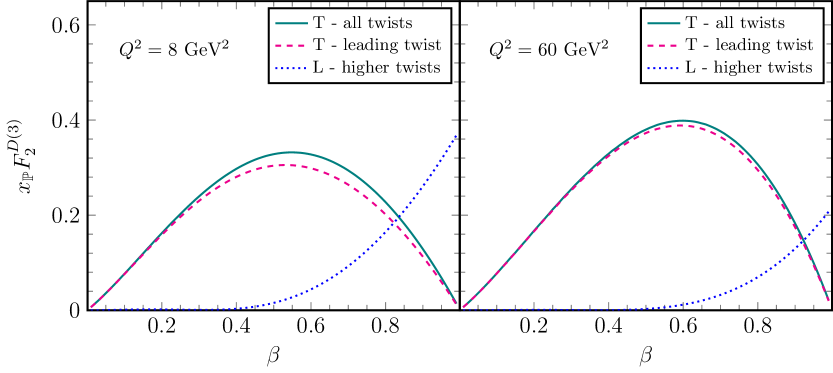
Figure 4: Transverse (all twist and its leading twist approximation) and longitudinal contributions to the diffractive structure function $x_{\mathbb{P}}F_{2}^{D(3)}$ as functions of $\beta$ for two representative values of $Q^{2}$. The scattering amplitude is given by the MV model with a saturation scale $Q_{s}^{2}=0.88\,\mathrm{GeV}^{2}$ (in the fundamental representation). A factor $S_{\perp}/4\pi^{3}$ has been omitted.

3 Diffractive (2+1)–jets with a soft quark

The discussion in the previous section shows that the typical dijets produced via elastic scattering are semi-hard, with transverse momenta $K_{\perp}\sim Q_{s}(Y_{\mathbb{P}})$, even when the virtual photon is much harder, $Q^{2}\gg Q_{s}^{2}(Y_{\mathbb{P}})$. The cross-section for producing much harder jets, with $P_{\perp}\gg Q_{s}$, decreases very fast, like $1/P_{\perp}^{6}$ (see Eq. (204) in Appendix B for a succinct discussion and also App. A in Ref. Iancu:2022lcw for more details). For dijet production, this $1/P_{\perp}^{6}$ spectrum should be viewed as a higher-twist effect; for comparison, the inclusive production of a pair of jets in DIS leads to the harder spectrum $1/P_{\perp}^{4}$ Dominguez:2011wm . The ultimate reason for the strong suppression of hard exclusive dijets is the colour transparency of small dipoles: a hard $q\bar{q}$ pair has a small transverse size, hence it interacts only weakly.

However, all that is strictly true only so long as one stays at leading order in QCD perturbation theory, that is, if one limits oneself to the exclusive production of a quark-antiquark pair. As originally observed in Iancu:2021rup , a pair of hard jets with relative transverse momentum $P_{\perp}\gg Q_{s}$ can be efficiently produced via coherent diffraction if one allows for the formation of a third, semi-hard, jet, with transverse momentum $K_{\perp}\sim Q_{s}$. Such a “(2+1)–jet” process starts with a $q\bar{q}g$ fluctuation of the virtual photon, hence the respective cross-section is suppressed by a power of $\alpha_{s}$. Yet, the ensuing spectrum for the hard dijets decays only like $1/P_{\perp}^{4}$ and thus dominates over the exclusive $q\bar{q}$ production at large $P_{\perp}$. The emergence of this harder spectrum is closely connected to the presence of the third jet in the final state, with $K_{\perp}\sim Q_{s}$: because of the latter, the overall transverse size $R$ of the $q\bar{q}g$ fluctuation is quite large, $R\sim 1/Q_{s}$, despite the fact that two of the jets are hard. This allows for strong scattering in the black disk limit and thus avoids the suppression due to colour transparency.

The Feynman graphs in Figs. 5 and 6 illustrate the leading-order amplitudes for different final states with 2+1 “jets” (actually, partons). In Fig. 5 the final gluon is semi-hard, while the hard dijet is made with the quark and the antiquark ($q\bar{q}$). The total amplitude for this process is the sum of the two contributions, since the gluon can be emitted by the quark (left panel) or the antiquark (right panel). For the two other processes, as shown in Fig. 6, the final state includes a hard antiquark-gluon ($\bar{q}g$) dijet together with a semi-hard quark. (There are of course similar processes where the semi-hard final “jet” is the antiquark.) Once again, the gluon can be emitted by either the quark, or the antiquark, but since the two fermions have widely different kinematics — in the final state, one is hard, while the other one is semi-hard —, the respective amplitudes have different properties and need be separately computed. These two amplitudes interfere with each other (since they lead to the same final state), hence they must be added before computing the cross-section.

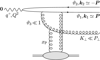
Figure 5: Diffractive scattering with a final state composed of a hard $q\bar{q}$ dijet and a semi-hard gluon. The gluon is emitted either from the quark (left panel) or from the antiquark (right panel) and at a large transverse distance $R\sim 1/K_{\perp}$ from the small $q\bar{q}$ pair (with transverse size $r\sim 1/P_{\perp}$).

Our drawing of the three amplitudes in Figs. 5 and 6 is meant to emphasise their space-time structure and, especially, their distribution in the transverse coordinate space, which in turn reflects the kinematics of the final state. In all these cases, one observes a large transverse separation $R\sim 1/K_{\perp}$ with, typically, $K_{\perp}\sim Q_{s}(Y_{\mathbb{P}})$, between the semi-hard parton and the hard dijet, which is relatively compact, with transverse size $r\sim 1/P_{\perp}\ll 1/Q_{s}$. Since $1/Q_{s}$ is also the typical scale for transverse variations in the gluon distribution of the target, it should be clear that, in so far as the scattering is concerned, the small dijet can be effectively treated as a point-like particle in the appropriate representation of the colour group SU($N_{c}$). For instance, in the case of a semi-hard gluon, cf. Fig. 5, the hard $q\bar{q}$ pair scatters like an effective gluon and the amplitude is proportional to the elastic scattering amplitude $\mathcal{T}_{g}(R,Y_{\mathbb{P}})$ of a gluon-gluon dipole with large size $R\sim 1/Q_{s}$ (which is of order one, as anticipated). Similarly, for the diagrams with a soft quark in Fig. 6, one encounters an effective quark-antiquark dipole, with elastic scattering amplitude $\mathcal{T}_{q\bar{q}}(R,Y_{\mathbb{P}})\sim\mathcal{O}{\left(1\right)}$.

Notice that the photon virtuality $Q^{2}$ plays no special role in these arguments: so long as $P_{\perp}\gg Q_{s}$, the dijet is hard irrespective of the photon virtuality and our subsequent analysis holds for arbitrary values of $Q^{2}$ (including the photo-production limit $Q^{2}\to 0$). Yet, for the sake of the discussion, we shall often treat $Q^{2}$ as a hard scale which is comparable to $P_{\perp}^{2}$.

The (2+1)–jet process with a semi-hard gluon has been discussed in detail in Iancu:2021rup ; Iancu:2022lcw (see also Refs. Wusthoff:1997fz ; GolecBiernat:1999qd ; Hebecker:1997gp ; Buchmuller:1998jv ; Hautmann:1998xn ; Hautmann:1999ui ; Hautmann:2000pw ; Golec-Biernat:2001gyl for earlier related work), with results that will be briefly summarised in the next subsection. After that, we will present the corresponding analysis for the processes involving a semi-hard quark. Before we proceed, let us specify our notations and conventions. We shall use the subscripts 1, 2, and 3 to label the momenta of the quark, antiquark, and gluon respectively. The “plus” components of their 4-momenta will be written as $k_{i}^{+}=\vartheta_{i}q^{+}$, with $\vartheta_{1}+\vartheta_{2}+\vartheta_{3}=1$. For coherent diffraction, we can neglect the transverse momentum transferred by the target, which implies $\bm{k}_{1}+\bm{k}_{2}+\bm{k}_{3}=0$. Two of these jets are hard, while the third one is semi-hard. By momentum conservation, the hard dijets propagate back-to-back in the transverse plane: their relative transverse momentum $P_{\perp}$ is much larger than their momentum imbalance $K_{\perp}$, which is fixed by the third jet. For instance, for the process with a semi-hard gluon in Fig. 5, we have $P_{\perp}\gg K_{\perp}$, where $P_{\perp}\simeq k_{1\perp}\simeq k_{2\perp}$ and $K_{\perp}\equiv|\bm{k}_{1}+\bm{k}_{2}|=k_{3\perp}$.

A final point, which is important for what follows: besides being “semi-hard”, in the sense of having a transverse momentum $K_{\perp}\sim Q_{s}(Y_{\mathbb{P}})$, the third jet is also soft, in the sense of carrying a small fraction $\vartheta\sim K_{\perp}^{2}/P_{\perp}^{2}\ll 1$ of the longitudinal momentum $q^{+}$ of the incoming photon. This property follows from formation time constraints, and more precisely from the condition to have a large effective dipole at the time of scattering (see below for details). Because of this, it becomes possible to factorise out this semi-hard parton from the hard dijet and to reinterpret it as a part of the target wavefunction — very much like the factorisation of the soft quark from the $q\bar{q}$ pair in the calculation of SIDIS in the previous section. This factorisation has been demonstrated in Refs. Iancu:2021rup ; Iancu:2022lcw for (2+1)–jets with a soft gluon and will be extended below to the corresponding processes with a soft fermion. To summarise, the third jet is both semi-hard and soft, and will often be referred to as “the soft jet” (or “the semi-hard jet”), for brevity.

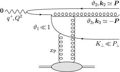
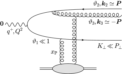
Figure 6: Diffractive scattering with a final state composed of a hard $\bar{q}g$ dijet and a semi-hard quark. The gluon is emitted either from the quark (left panel) or from the antiquark (right panel). The quark is always far from the small $\bar{q}g$ dijet.

3.1 2+1 jets with a soft gluon: a brief review

This case is illustrated by the amplitude in Fig. 5: the quark-antiquark pair is hard and nearly back-to-back, $k_{1\perp}\simeq k_{2\perp}\gg Q_{s}(Y_{\mathbb{P}})$, whereas the gluon is semi-hard, $k_{3\perp}\sim Q_{s}(Y_{\mathbb{P}})$, and also soft: $\vartheta_{3}\ll 1$. As already mentioned, this particular case has been studied in great detail in Iancu:2021rup ; Iancu:2022lcw , from which we quote here the final results. We recall that there are only two independent momentum variables, conveniently chosen as

$$\bm{P}\equiv\frac{\vartheta_{1}\bm{k}_{2}-\vartheta_{2}\bm{k}_{1}}{\vartheta_{1}+\vartheta_{2}}\simeq\vartheta_{1}\bm{k}_{2}-\vartheta_{2}\bm{k}_{1}\,,\qquad\bm{K}\equiv\bm{k}_{1}+\bm{k}_{2},$$ (56)

where we have also used $\vartheta_{3}\ll 1$, hence $\vartheta_{1}+\vartheta_{2}\simeq 1$. Physically, $\bm{P}$ is the relative momentum of the hard $q\bar{q}$ pair, $\bm{K}$ is their imbalance, and $\bm{k}_{3}=-\bm{K}$.

To start with, let us clarify the physical origin of the softness condition $\vartheta_{3}\ll 1$. In order for the scattering to be strong, the gluon must be emitted before the collision with the nuclear target. That is, its formation time $\tau_{g}\simeq 2\vartheta_{3}q^{+}/k_{3\perp}^{2}$ must be smaller than the photon coherence time $\tau_{\gamma}=2q^{+}/Q^{2}$ (the lifetime of the $q\bar{q}$ fluctuation in the absence of scattering). This is satisfied provided $\vartheta_{3}\lesssim K_{\perp}^{2}/Q^{2}$, which is indeed small for the interesting values $Q^{2}\gg K_{\perp}^{2}\sim Q_{s}^{2}$. A similar condition holds when the photon is real ($Q^{2}\to 0$): in that case the lifetime of the $q\bar{q}$ pair is estimated as $\tau_{q\bar{q}}\simeq 2\vartheta_{1}\vartheta_{2}q^{+}/P_{\perp}^{2}$ and the softness condition becomes $\vartheta_{3}\lesssim K_{\perp}^{2}/P_{\perp}^{2}$. (We generally treat $\vartheta_{1}$ and $\vartheta_{2}$ as comparable quantities of order 1/2, but asymmetric configurations with $\vartheta_{1}\vartheta_{2}\ll 1$ will be interesting in special cases.)

Yet, when computing the amplitude, it is not always possible to work in the lowest order approximation in $\vartheta_{3}$ (e.g. one cannot treat the gluon emission vertex in the eikonal approximation): the subleading corrections become important for the largest allowed values $\vartheta_{3}\sim K_{\perp}^{2}/P_{\perp}^{2}$, which are the most interesting in practice Iancu:2022lcw . This is related to the fact that the would-be leading-order contributions in the double limit $\vartheta_{3}\to 0$ and $K_{\perp}\to 0$ precisely cancel between the two amplitudes representing gluon emission from the quark and, respectively, the antiquark. So, one needs to keep terms of next-to-leading order in either $\vartheta_{3}$, or $K_{\perp}/P_{\perp}$, and the respective contributions are comparable to each other for the interesting values $\vartheta_{3}\sim K_{\perp}^{2}/P_{\perp}^{2}$ (see Sect. 4 in Iancu:2022lcw for details).

This argument also has important consequences for the new analysis in this paper: it explains why the diffractive production of (2+1)–jets with a soft quark is not suppressed compared to the respective process with a soft gluon, despite the fact that the latter is a priori favoured by the soft singularity of bremsstrahlung: this enhancement is in practice compensated by the dipolar nature of the soft gluon radiation, i.e. by the fact that the gluon can be emitted by either the quark, or the antiquark, and these two emitters partially screen each other when seen from large distances. These compensation is fully effective only when $\vartheta_{3}\sim K_{\perp}^{2}/P_{\perp}^{2}$. The (2+1)–processes which involve much softer gluons with $\vartheta_{3}\ll K_{\perp}^{2}/P_{\perp}^{2}$ are still dominant, but they are less interesting since they have lower rapidity gaps. To understand this, let us examine the rapidity gap $Y_{\mathbb{P}}=\ln(1/x_{\mathbb{P}})$ for the $q\bar{q}g$ final state: one can write (cf. Eq. (1))

$$x_{\mathbb{P}}=\frac{1}{2q^{+}P_{N}^{-}}\left(\frac{k^{2}_{1\perp}}{\vartheta_{1}}+\frac{k^{2}_{2\perp}}{\vartheta_{2}}+\frac{k^{2}_{3\perp}}{\vartheta_{3}}+Q^{2}\right)\geq x_{q\bar{q}},$$ (57)

where $x_{q\bar{q}}P_{N}^{-}$ is the light-cone energy needed to put the hard $q\bar{q}$ pair on-shell:

$$x_{q\bar{q}}=\frac{1}{2q^{+}P_{N}^{-}}\left(\frac{k^{2}_{1\perp}}{\vartheta_{1}}+\frac{k^{2}_{2\perp}}{\vartheta_{2}}+Q^{2}\right)\,\simeq\,\frac{1}{\hat{s}}\left(\frac{P_{\perp}^{2}}{\vartheta_{1}\vartheta_{2}}+Q^{2}\right)\,.$$ (58)

The quantity $Y_{q\bar{q}}\equiv\ln(1/x_{q\bar{q}})$ — that is, the rapidity separation between the $q\bar{q}$ dijet and the target — provides an upper limit on the rapidity gap $Y_{\mathbb{P}}$. So long as $\vartheta_{3}\sim K_{\perp}^{2}/P_{\perp}^{2}$, $x_{\mathbb{P}}$ and $x_{q\bar{q}}$ are comparable with each other, hence $Y_{\mathbb{P}}$ is close to its maximal value $Y_{q\bar{q}}$. But for much softer gluons with $\vartheta_{3}\ll K_{\perp}^{2}/P_{\perp}^{2}$, the rapidity gap $Y_{\mathbb{P}}$ is considerably smaller than $Y_{q\bar{q}}$, and then the process is less interesting (e.g. it is less favourable to gluon saturation). In fact, such very soft gluons should more naturally be seen as part of the high-energy evolution of the projectile Kovchegov:1999ji ; Hatta:2006hs .

The strong separation of scales, both transverse and longitudinal, between the semi-hard gluon and the hard $q\bar{q}$ pair leads to important simplifications which allows one to write the cross-section for diffractive (2+1)–jet production in the TMD factorised form Iancu:2022lcw

$$\frac{{\rm d}\sigma^{\gamma_{T,L}^{*}A\rightarrow q\bar{q}(g)A}}{{\rm d}\vartheta_{1}{\rm d}\vartheta_{2}{\rm d}^{2}\!\bm{P}{\rm d}^{2}\!\bm{K}{\rm d}Y_{\mathbb{P}}}=\tilde{H}_{T,L}(\vartheta_{1},\vartheta_{2},{Q}^{2},P_{\perp}^{2})\,\frac{{\rm d}xG_{\mathbb{P}}(x,x_{\mathbb{P}},K_{\perp}^{2})}{{\rm d}^{2}\bm{K}},$$ (59)

which is further illustrated in the right panel in Fig. 7. The final state is indicated as $q\bar{q}(g)A$ with the gluon label shown in parentheses, to emphasise that this is the soft parton in the final state. The “hard factors” have been defined as (with $\bar{Q}^{2}=\vartheta_{1}\vartheta_{2}{Q}^{2}$)

$$\tilde{H}_{T}(\vartheta_{1},\vartheta_{2},{Q}^{2},P_{\perp}^{2})\equiv{\alpha_{em}\alpha_{s}}\Big{(}\sum e_{f}^{2}\Big{)}\,\delta(1-\vartheta_{1}-\vartheta_{2})\left(\vartheta_{1}^{2}+\vartheta_{2}^{2}\right)\frac{P_{\perp}^{4}+\bar{Q}^{4}}{(P_{\perp}^{2}+\bar{Q}^{2})^{4}}\,$$ (60)

for a photon with transverse polarisation and, respectively,

$$\tilde{H}_{L}(\vartheta_{1},\vartheta_{2},{Q}^{2},P_{\perp}^{2})\equiv{\alpha_{em}\alpha_{s}}\Big{(}\sum e_{f}^{2}\Big{)}\,\delta(1-\vartheta_{1}-\vartheta_{2})\vartheta_{1}\vartheta_{2}\,\frac{8P_{\perp}^{2}\bar{Q}^{2}}{(P_{\perp}^{2}+\bar{Q}^{2})^{4}}\,$$ (61)

for the case of a longitudinal photon. If $P_{\perp}^{2}$ and $\bar{Q}^{2}$ are of the same order, then, clearly, both $\tilde{H}_{T}$ and $\tilde{H}_{L}$ decrease like $1/P_{\perp}^{4}$, as anticipated. On the other hand, if $P_{\perp}^{2}\gg\bar{Q}^{2}$, then $\tilde{H}_{T}$ is still proportional to $1/P_{\perp}^{4}$, but $\tilde{H}_{L}$ decreases faster, like $\bar{Q}^{2}/P_{\perp}^{6}$, and thus becomes negligible. In particular, the longitudinal contribution vanishes for a real photon ($Q^{2}\to 0$), unlike $\tilde{H}_{T}$, which has a finite value in that limit.

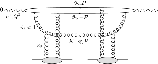
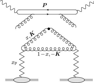
Figure 7: Diagrams representing the cross-section for the diffractive production of (2+1)–jets with a soft gluon. Left panel: the viewpoint of the colour dipole picture. Right panel: the TMD factorisation of the soft gluon from the hard $q\bar{q}$ pair.

Furthermore, the “semi-hard factor” in Eq. (59) is the gluon diffractive TMD, defined as (compare to Eq. (34))

$$\frac{{\rm d}xG_{\mathbb{P}}(x,x_{\mathbb{P}},K_{\perp}^{2})}{{\rm d}^{2}\bm{K}}\equiv\frac{S_{\perp}(N_{c}^{2}-1)}{4\pi^{3}}\,\frac{[\mathcal{G}_{\mathbb{P}}(x,x_{\mathbb{P}},K_{\perp}^{2})]^{2}}{2\pi(1-x)}\equiv\frac{S_{\perp}(N_{c}^{2}-1)}{4\pi^{3}}\,\Phi_{\mathbb{P}}(x,x_{\mathbb{P}},K_{\perp}^{2})$$ (62)

with (below, $\mathcal{M}^{2}=\frac{x}{1-x}K_{\perp}^{2}$)

$$\mathcal{G}_{\mathbb{P}}(x,x_{\mathbb{P}},K_{\perp}^{2})=\mathcal{M}^{2}\int_{0}^{\infty}{\rm d}R\,R\,J_{2}(K_{\perp}R)K_{2}(\mathcal{M}R)\mathcal{T}_{g}(R,Y_{\mathbb{P}}).$$ (63)

The hard factors describe the formation of the $q\bar{q}$ pair and its coupling to a $t$-channel gluon produced by the Pomeron. The gluon DTMD represents the unintegrated gluon distribution of the Pomeron, i.e. the number of gluons in the Pomeron wavefunction which have a transverse momentum $K_{\perp}$ and a “minus” longitudinal momentum fraction $x$ w.r.t. the Pomeron. In particular, $\Phi_{\mathbb{P}}$ denotes the gluon occupation number in the Pomeron.

When computing the cross-section (59), $x$ is not an independent variable. Rather, its value is fixed by the diffractive gap together with the kinematics of the hard dijet, via (recall Eq. (58))

$$x=\frac{x_{q\bar{q}}}{x_{\mathbb{P}}}\,=\,\beta\,\frac{x_{q\bar{q}}}{x_{\rm\scriptscriptstyle Bj}}\,\simeq\,\beta\,\frac{\bar{Q}^{2}+P_{\perp}^{2}}{\bar{Q}^{2}}\,.$$ (64)

To get more insight into the gluon distribution of the Pomeron, it is useful to have a piecewise approximation to the gluon occupation number, like Eq. (52) for the quark occupation number. Via manipulations similar to those in Sect. 2.5, one finds Iancu:2021rup ; Iancu:2022lcw

$$\Phi_{\mathbb{P}}(x,x_{\mathbb{P}},K_{\perp}^{2})\,\simeq\frac{1-x}{2\pi}\begin{cases}\displaystyle{\ 1}&\text{for \ $K_{\perp}\!\ll\tilde{Q}_{s,g}(x,Y_{\mathbb{P}})$}\\[11.38092pt] \displaystyle{\ \frac{\tilde{Q}_{s,g}^{4}(x,Y_{\mathbb{P}})}{K_{\perp}^{4}}}&\text{for \ $K_{\perp}\!\gg\tilde{Q}_{s,g}(x,Y_{\mathbb{P}})$}\,.\end{cases}$$ (65)

with $\tilde{Q}_{s,g}^{2}(x,Y_{\mathbb{P}})=(1-x)Q_{s,g}^{2}(Y_{\mathbb{P}})$, where $Q_{s,g}(Y_{\mathbb{P}})$ is the value of the saturation momentum probed by a gluon-gluon dipole. It is approximately related to the corresponding value for a $q\bar{q}$ dipole via the ratio of the respective Casimir factors: $Q_{s,g}^{2}(Y_{\mathbb{P}})\simeq(N_{c}/C_{F})Q_{s}^{2}(Y_{\mathbb{P}})\simeq 2Q_{s}^{2}(Y_{\mathbb{P}})$.

Eq. (65) is similar to Eq. (52) in the sense that they both show saturation at low momenta and a rapidly decaying tail $\propto 1/K_{\perp}^{4}$ at high momenta. Note however the different dependence upon $x$: the gluon occupation number is non-zero when $x\to 0$, but it vanishes faster when $x\to 1$.

If one is not interested in measuring the transverse momentum imbalance of the hard dijets (hence, neither the momentum $K_{\perp}$ of the gluon jet), then one can integrate the cross-section (59) over $K_{\perp}$ up to an upper limit of order $P_{\perp}$. Clearly, this operation produces the gluon distribution of the Pomeron (a.k.a. the gluon diffractive PDF) on the resolution scale $\sim P_{\perp}^{2}$. One finds

$$\frac{{\rm d}\sigma^{\gamma_{T,L}^{*}A\rightarrow q\bar{q}(g)A}}{{\rm d}\vartheta_{1}{\rm d}\vartheta_{2}{\rm d}^{2}\!\bm{P}{\rm d}Y_{\mathbb{P}}}=\tilde{H}_{T,L}(\vartheta_{1},\vartheta_{2},{Q}^{2},P_{\perp}^{2})\,xG_{\mathbb{P}}(x,x_{\mathbb{P}},(1-x)P_{\perp}^{2}),$$ (66)

with the following approximation for the gluon DPDF:

$$xG_{\mathbb{P}}(x,x_{\mathbb{P}},Q^{2})\equiv\int{\rm d}^{2}\bm{K}\,\frac{{\rm d}xG_{\mathbb{P}}(x,x_{\mathbb{P}},K_{\perp}^{2})}{{\rm d}^{2}\bm{K}}=\frac{S_{\perp}(N_{c}^{2}-1)}{4\pi^{2}}\int_{0}^{Q^{2}}\!{\rm d}K_{\perp}^{2}\,\Phi_{\mathbb{P}}(x,x_{\mathbb{P}},K_{\perp}^{2}).$$ (67)

The precise value of the resolution scale which appears in Eq. (66), namely $(1-x)P_{\perp}^{2}$, will be justified later (see the discussion after Eq. (131)), but it is not very important at this point: given the rapid decay of the integrand in (67) at large momenta $K_{\perp}\gg\tilde{Q}_{s,g}(x,Y_{\mathbb{P}})$, cf. Eq. (65), it is clear that the result of the integral is quasi-independent of its upper limit $Q^{2}$ so long as $Q^{2}\gg\tilde{Q}_{s,g}^{2}(x,Y_{\mathbb{P}})$.

Using (65), one finds a simple approximation (compare to Eq. (55)),

$$xG_{\mathbb{P}}(x,x_{\mathbb{P}},Q^{2})=\frac{S_{\perp}(N_{c}^{2}-1)}{4\pi^{3}}\,\kappa_{g}(1-x)^{2}{Q}_{s,g}^{2}(Y_{\mathbb{P}}),$$ (68)

with $\kappa_{g}\sim\mathcal{O}{\left(1\right)}$, which can be useful for parametric estimates.

When the resolution scale $Q^{2}$ in Eq. (67) is so large that $\alpha_{s}\ln(Q^{2}/Q_{s,g}^{2}(Y_{\mathbb{P}}))\sim 1$, one expects the present approximation to be modified by the effects of the DGLAP evolution. We shall return to this point after computing the cross-sections for the diffractive (2+1)–jet processes with a soft quark.

3.2 2+1 jets with a soft quark: gluon emission from the antiquark

As mentioned at the beginning of this section, we consider the configurations illustrated in Fig. 6, where the final state includes a hard antiquark-gluon ($\bar{q}g$) dijet together with a semi-hard quark ($q$). We shall separately compute the amplitudes corresponding to these two configurations, starting with the case where the gluon is emitted by the antiquark. As suggested by the graphical representation of the respective amplitude in the right panel in Fig. 6, this is the case where the $q\bar{q}$ dipole produced by the decay of the virtual photon is relatively large, with a typical transverse size $R\sim 1/Q_{s}$.

Before specialising to that case, we briefly review the calculation of the three-parton ($q\bar{q}g$) component of the light-cone wavefunction (LCWF) of the virtual photon. The LCWF is measured at LC time $x^{+}\to\infty$, whereas the scattering with the nuclear shockwave (SW) is localised near $x^{+}=0$. There are three possible time orderings: (1) both the photon decay and the gluon emission occur at negative $x^{+}$ (before the scattering with the SW), (2) the photon decays before crossing the SW ($x^{+}<0$) , but the gluon is emitted only after ($x^{+}>0$), and (3) the photon decays after crossing the SW ($x^{+}>0$). In case (1), all the three partons can interact with the target. In case (2), it is only the initial $q\bar{q}$ fluctuation which can interact. Finally, in case (3), there is no interaction at all.

In the absence of any scattering (that is, if there is no SW at $x^{+}=0$), the three contributions to the LCWF must add to zero: indeed, a space-like (or even light-like) photon cannot decay into an on-shell partonic system, by energy-momentum conservation. Thus, when computing the full LCWF (including the scattering with the SW), it suffices to consider the first two time-orderings above; the third case can be simply accounted for by subtracting the no-scattering limits from the two other cases. We would like to point out that in addition to the aforementioned possibilities, according to the rules of LCPT one should also take into account diagrams with instantaneous interactions. In general, the latter contribute to the LCWF under consideration, however they are suppressed in the particular kinematics we are interested in, as we show in Appendix C.

As anticipated, we are interested in three-parton configurations which are quite special: a hard antiquark-gluon pair accompanied by a quark which is both soft ($\vartheta_{1}\ll 1$) and semi-hard ($k_{1\perp}\sim Q_{s}$). This special kinematics allows for important simplifications, that are most conveniently implemented by working in the momentum space representation. On the other hand, the (multiple) scattering with the nuclear target is easier to include in the transverse coordinate representation, where the eikonal approximation takes a simple form. Accordingly, our strategy in this section will be as follows. We shall first compute the momentum-space $q\bar{q}g$ components of the photon LCWF corresponding to the first two time-orderings above and in the absence of scattering. We shall then identify and implement the relevant kinematical approximations, as permitted by the special structure of the final state. Finally, we shall change representation (from transverse momenta to transverse coordinates) via a Fourier transform and include the effects of the scattering in the eikonal approximation.

The general structure of the $q\bar{q}g$ component of the virtual photon LCWF in the absence of scattering and in momentum space reads as follows (compare to the $q\bar{q}$ component in Eq. (2.2))

$$\big{|}\gamma_{\scriptscriptstyle T}^{i}\big{\rangle}_{q\bar{q}g}=\,t^{a}_{\alpha\beta}\int_{0}^{1} {\rm d}\vartheta_{1}{\rm d}\vartheta_{2}\,{\rm d}\vartheta_{3}\,\delta(1-\vartheta_{1}-\vartheta_{2}-\vartheta_{3})\int{\rm d}^{2}\bm{k}_{1}\,{\rm d}^{2}\bm{k}_{2}\,{\rm d}^{2}\bm{k}_{3}\,\delta^{(2)}(\bm{k}_{1}+\bm{k}_{2}+\bm{k}_{3})$$

$$\times\Psi^{im}_{\lambda_{1}\lambda_{2}}(\vartheta_{1},\bm{k}_{1},\vartheta_{2},\bm{k}_{2},\vartheta_{3},\bm{k}_{3})\,\big{|}{q}_{\lambda_{1}}^{\alpha}(\vartheta_{1},\bm{k}_{1})\,\bar{q}_{\lambda_{2}}^{\beta}(\vartheta_{2},\bm{k}_{2})\,g_{m}^{a}(\vartheta_{3},\bm{k}_{3})\big{\rangle}.$$ (69)

The notation related to the two fermions is the same as the one used in the previous section starting from Eq. (2.2). In addition, $\bm{k}_{3}$, $\vartheta_{3}$, $a$ and $m=1,2$ stand respectively for the transverse momentum, longitudinal fraction (w.r.t. the virtual photon), color index and polarisation state of the transverse gluon. The gluon can be emitted by either the antiquark, or the quark, and its emission can occur either before, or after, the scattering with the SW. Accordingly, the probability amplitude $\Psi^{im}_{\lambda_{1}\lambda_{2}}$ receives several contributions, that will be computed in what follows. Similar calculations can be found in the literature, so in practice we shall simply adapt the results of Ref. Iancu:2022gpw to the kinematical conditions of interest.

In this section we consider the case where the gluon is emitted by the antiquark, so we shall insert a lower label “($\bar{q}$)” on the respective components of the amplitude. There are two possible time-orderings (with time $t\equiv x^{+}$), see Fig. 8: (1) the photon decays at some time $t_{1}<0$ and the gluon is then emitted at a time $t_{2}$ which is negative as well, $t_{1}<t_{2}<0$, and (2) the photon decays at time $t_{1}<0$, but the gluon is emitted at some positive time $t_{2}>0$. The integrals over $t_{1}$ and $t_{2}$ generate the energy denominators, which are different in the two cases Iancu:2022gpw .

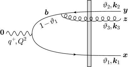
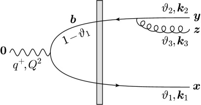
Figure 8: The amplitude for (2+1)-jet production in DIS off a nuclear shockwave via the channel $\bar{q}^{\prime}\to\bar{q}g$. The large pair is formed already at the photon vertex. Left panel: The gluon is radiated before the scattering off the shockwave. Right panel: The gluon is radiated after the scattering off the shockwave.

When the gluon is emitted prior to the scattering ($t_{1}<t_{2}<0$), the amplitude in momentum space and in absence of the scattering takes the following form Iancu:2022gpw .

$$\Psi^{im\,(1)}_{\lambda_{1}\lambda_{2}\,(\bar{q})}=\delta_{\lambda_{1}\lambda_{2}}\,\frac{1}{8q^{+}}\,\frac{ee_{f}g}{(2\pi)^{6}}\,\frac{1}{\vartheta_{1}(1-\vartheta_{1})\vartheta_{2}\vartheta_{3}}\,\frac{1}{\sqrt{\vartheta_{3}}}\,\frac{\varphi^{ij}(\vartheta_{1},\lambda_{1})\,k_{1}^{j}}{E_{q}+E_{\bar{q}^{\prime}}-E_{\gamma}}\,\frac{\tau^{mn}(\vartheta_{1},\vartheta_{2},\lambda_{1})P^{n}}{E_{q}+E_{\bar{q}}+E_{g}-E_{\gamma}}.$$ (70)

The LC energies in the denominators in Eq. (70) read

$$E_{q}=\frac{k_{1\perp}^{2}}{2\vartheta_{1}q^{+}},\quad E_{\bar{q}}=\frac{k_{2\perp}^{2}}{2\vartheta_{2}q^{+}},\quad E_{g}=\frac{k_{3\perp}^{2}}{2\vartheta_{3}q^{+}},\quad E_{\bar{q}^{\prime}}=\frac{k_{1\perp}^{2}}{2(1-\vartheta_{1})q^{+}},\quad E_{\gamma}=-\frac{Q^{2}}{2q^{+}},$$ (71)

where we have denoted with a prime the antiquark in the intermediate state (before the gluon emission). The first energy denominator is generated by the photon decay, while the second one corresponds to the gluon emission. The function $\varphi^{ij}(\vartheta,\lambda)$ has been defined in Eq. (8), while the new function

$$\tau^{mn}(\vartheta_{1},\vartheta_{2},\lambda)\equiv(1-\vartheta_{1}+\vartheta_{2})\delta^{mn}+2i\lambda\vartheta_{3}\varepsilon^{mn}$$ (72)

with $\vartheta_{3}=1\!-\!\vartheta_{1}\!-\!\vartheta_{2}$, arises from the polarization structure of the $\bar{q}\to\bar{q}g$ vertex. The latter is also proportional to the relative transverse velocity of the two daughter partons, that is

$$\frac{1}{\vartheta_{2}+\vartheta_{3}}\left(\frac{\bm{k}_{2}}{\vartheta_{2}}-\frac{\bm{k}_{3}}{\vartheta_{3}}\right)=\,\frac{\bm{P}}{\vartheta_{2}\vartheta_{3}}\,\Longleftrightarrow\,\bm{P}\equiv\frac{\vartheta_{3}\bm{k}_{2}-\vartheta_{2}\bm{k}_{3}}{\vartheta_{2}+\vartheta_{3}},$$ (73)

where $\bm{P}$ is the relative momentum of the $\bar{q}g$ pair, which also appears in Eq. (70). For what follows, it is convenient to choose $\bm{P}$ and $\bm{k}_{1}$ as independent momenta and express $\bm{k}_{2}$ and $\bm{k}_{3}$ in terms of them (by also using the condition of transverse momentum conservation: $\bm{k}_{1}+\bm{k}_{2}+\bm{k}_{3}=\bm{0}$):

$$\bm{k}_{2}=\bm{P}-\frac{\vartheta_{2}\bm{k}_{1}}{\vartheta_{2}+\vartheta_{3}},\qquad\bm{k}_{3}=-\bm{P}-\frac{\vartheta_{3}\bm{k}_{1}}{\vartheta_{2}+\vartheta_{3}}.$$ (74)

When the gluon emission occurs at positive times ($t_{1}<0<t_{2}$), the amplitude differs from the one in Eq. (70) only in the second energy denominator, which now involves the LC energy difference between the intermediate $q\bar{q}$ state and the final $q\bar{q}g$ one, that is Iancu:2022gpw ,

$$\Psi^{im\,(2)}_{\lambda_{1}\lambda_{2}\,(\bar{q})}=\delta_{\lambda_{1}\lambda_{2}}\,\frac{1}{8q^{+}}\,\frac{ee_{f}g}{(2\pi)^{6}}\,\frac{1}{\vartheta_{1}(1-\vartheta_{1})\vartheta_{2}\vartheta_{3}}\,\frac{1}{\sqrt{\vartheta_{3}}}\,\frac{\varphi^{ij}(\vartheta_{1},\lambda_{1})\,k_{1}^{j}}{E_{q}+E_{\bar{q}^{\prime}}-E_{\gamma}}\,\frac{\tau^{mn}(\vartheta_{1},\vartheta_{2},\lambda_{1})P^{n}}{E_{\bar{q}^{\prime}}-E_{\bar{q}}-E_{g}}.$$ (75)

At this level, one would now need to perform a Fourier transform to coordinate space, then insert the proper scattering $S$-matrices which are generally different for each of the two configurations and, only after that, sum the resulting probability amplitudes. However, this procedure can be considerably simplified for the problem at hand, as we now explain.

Recall that we are interested in special configurations where the antiquark and the gluon are hard, $P_{\perp}\gg Q_{s}(Y_{\mathbb{P}})$, whereas the quark is semi-hard, $k_{1\perp}\sim Q_{s}(Y_{\mathbb{P}})$. For such configurations, the overall size of the $q\bar{q}g$ system $R\sim 1/Q_{s}$ is much larger than the transverse separation $r\sim 1/P_{\perp}$ between the gluon and the antiquark. In particular, the $\bar{q}g$ pair is so small — its transverse size $r$ is much smaller than the correlation length $1/Q_{s}$ of the colour fields in the target — that it scatters in the same way as its parent antiquark $\bar{q}^{\prime}$. Hence, in so far as the scattering is concerned, there is no difference between the two time-orderings: in both cases, the partonic system scatters as a $q\bar{q}$ dipole with size $R$.

This allows us to add the respective amplitudes already in the absence of scattering, as shown (in momentum-space) in Eqs. (70) and (75). Their sum involves the following linear combination of energy denominators

$$\frac{1}{E_{q}+E_{\bar{q}^{\prime}}-E_{\gamma}}\!\left(\frac{1}{E_{q}+E_{\bar{q}}+E_{g}-E_{\gamma}}+\frac{1}{E_{\bar{q}^{\prime}}-E_{\bar{q}}-E_{g}}\right)=\frac{1}{E_{\bar{q}^{\prime}}-E_{\bar{q}}-E_{g}}\frac{1}{E_{q}+E_{\bar{q}}+E_{g}-E_{\gamma}},$$ (76)

whose result is formally the same as the product of energy denominators in the amplitude describing final-state evolution (the situation where both the photon decay and the gluon emission occur at positive times, $0<t_{1}<t_{2}$, after the photon crosses the shockwave). Making use of Eqs. (74) and (71) we immediately get

$$2q^{+}\big{(}E_{\bar{q}^{\prime}}-E_{\bar{q}}-E_{g}\big{)}=\frac{k_{1\perp}^{2}}{1-\vartheta_{1}}-\frac{k_{2\perp}^{2}}{\vartheta_{2}}-\frac{k_{3\perp}^{3}}{\vartheta_{3}}=-\frac{1-\vartheta_{1}}{\vartheta_{2}\vartheta_{3}}\,P_{\perp}^{2}\,\simeq-\frac{P_{\perp}^{2}}{\vartheta_{2}\vartheta_{3}},$$ (77)

and

$$2q^{+}\big{(}E_{q}+E_{\bar{q}}+E_{g}-E_{\gamma}\big{)} \,=\frac{k_{1\perp}^{2}}{\vartheta_{1}}+\frac{k_{2\perp}^{2}}{\vartheta_{2}}+\frac{k_{3\perp}^{2}}{\vartheta_{3}}+Q^{2}=\frac{k_{1\perp}^{2}}{\vartheta_{1}(1-\vartheta_{1})}+\frac{1-\vartheta_{1}}{\vartheta_{2}\vartheta_{3}}\,{P_{\perp}^{2}}+Q^{2}\,$$

$$\,\simeq\frac{k_{1\perp}^{2}+\mathcal{M}^{2}}{\vartheta_{1}},$$ (78)

where we have defined

$$\mathcal{M}^{2}\,\equiv\,\vartheta_{1}\left(\frac{P_{\perp}^{2}}{\vartheta_{2}\vartheta_{3}}+Q^{2}\right).$$ (79)

In writing the last approximate equalities in Eqs. (77) and (3.2) we have assumed the quark to be soft, that is, $\vartheta_{1}\ll 1$. This condition is needed to ensure that the quark transverse momentum remains relatively small, $k_{1\perp}\sim Q_{s}\ll P_{\perp}$, as required by strong scattering. Indeed, the typical values of $k_{1\perp}^{2}$ are fixed by the effective “mass-term” $\mathcal{M}^{2}$ in the energy denominator. Hence, in order for $k_{1\perp}$ to be semi-hard, we need $\mathcal{M}\sim Q_{s}$, which together with Eq. (79) implies $\vartheta_{1}\sim Q_{s}^{2}/P_{\perp}^{2}\ll 1$. In more physical terms, this condition on $\vartheta_{1}$ means that the lifetime $\tau_{q\bar{q}}\sim 2\vartheta_{1}q^{+}/k_{1\perp}^{2}$ of the intermediate $q\bar{q}$ state and the formation time $\tau_{q\bar{q}g}\sim 2q^{+}/P^{2}_{\perp}$ of the $q\bar{q}g$ system must be comparable to each other, so that they have comparable chances to scatter off the nuclear shockwave.

Notice that the r.h.s. of Eq. (79) involves a linear combination of $P_{\perp}^{2}$ and $Q^{2}$, which is hard provided at least one of these two scales is much larger than $Q_{s}^{2}$. So, all the results to be obtained in this section remain true in the photo-production limit $Q^{2}\to 0$, so long as $P_{\perp}^{2}$ is hard enough, of course.

Putting everything together, we find the total amplitude $\Psi^{im}_{\lambda_{1}\lambda_{2}\,(\bar{q})}=\Psi^{im\,(1)}_{\lambda_{1}\lambda_{2}\,(\bar{q})}+\Psi^{im\,(2)}_{\lambda_{1}\lambda_{2}\,(\bar{q})}$ in the absence of scattering:

$$\Psi^{im}_{\lambda_{1}\lambda_{2}\,(\bar{q})}\simeq-\,\delta_{\lambda_{1}\lambda_{2}}\,\frac{ee_{f}gq^{+}}{2(2\pi)^{6}}\,\frac{1}{\sqrt{\vartheta_{3}}}\,\frac{\varphi^{ij}(0,\lambda_{1})k_{1}^{j}}{k_{1\perp}^{2}+\mathcal{M}^{2}}\,\frac{\tau^{mn}(0,\vartheta_{2},\lambda_{1})P^{n}}{P_{\perp}^{2}}.$$ (80)

As anticipated, this depends only upon two transverse momentum variables: $\bm{k}_{1}$ and $\bm{P}$.

We are now in a position to add the effects of the scattering. To that aim, it is advantageous to change from the transverse momentum to the transverse coordinate representation. Let $\bm{x}$, $\bm{y}$ and $\bm{z}$ denote the transverse positions of the (final) quark, antiquark and gluon, respectively. It is convenient to change these variables to $\bm{r}$, $\bm{R}$ and $\bm{b}$, which are the transverse separation of the legs in the $\bar{q}g$ pair, the transverse separation of the legs in the $q\bar{q}^{\prime}$ pair (before the gluon emission), and the transverse position of the intermediate antiquark, respectively. We have

$$\bm{r}\equiv\bm{y}-\bm{z},\qquad\bm{R}\equiv\bm{x}-\bm{b},\qquad\bm{b}\equiv\frac{\vartheta_{2}\bm{y}+\vartheta_{3}\bm{z}}{\vartheta_{2}+\vartheta_{3}},$$ (81)

while the inverse transformation reads

$$\bm{x}=\bm{b}+\bm{R},\qquad\bm{y}=\bm{b}+\frac{\vartheta_{3}}{\vartheta_{2}+\vartheta_{3}}\,\bm{r},\qquad\bm{z}=\bm{b}-\frac{\vartheta_{2}}{\vartheta_{2}+\vartheta_{3}}\,\bm{r},$$ (82)

where, to the order of accuracy, one is allowed to let $\vartheta_{2}+\vartheta_{3}\simeq 1$. In terms of the new variables in Eqs. (73) and (82), the exponential phase which appears when performing the Fourier transform from momentum to coordinate space can be expressed as

$$\bm{k}_{1}\cdot\bm{x}+\bm{k}_{2}\cdot\bm{y}+\bm{k}_{3}\cdot\bm{z}\,=\,\bm{P}\cdot\bm{r}+\bm{k}_{1}\cdot\bm{R},$$ (83)

where we have made used of the fact that the total transverse momentum in the projectile wavefunction vanishes. (For coherent diffraction in which the target is homogeneous, this property remains true after adding the effects of the collision; recall e.g. the discussion in Sect. 2.)

Eq. (83) indicates that $\bm{r}$ is the dual variable to the hard momentum $\bm{P}$ and similarly $\bm{R}$ is dual to the semi-hard momentum $\bm{k}_{1}$, so we have that $r\ll R$. Moreover, from Eq. (82) we readily find that the recoil $|\bm{y}-\bm{b}|$ of the antiquark (due to the gluon emission) is of the order of $r$. We conclude that the gluon and the antiquark (both before and after the emission) are effectively at the same transverse position when “seen” by the quark, which is separated from the other partons by a large distance $R$ (see Fig. 8):

$$\bm{z}\simeq\bm{y}\simeq\bm{b}=\bm{x}-\bm{R}$$ (84)

Using this, one can check that the effect of the collision is indeed the same for both time orderings. Indeed, consider case (1) in which the gluon is emitted at $x^{+}<0$, hence it participates in the scattering. Before doing any diffractive projection, one can include the effect of the collision by replacing (analogously to Eq. (15))

$$t^{a}_{\alpha\beta}\to\big{[}U^{ab}(\bm{z})V(\bm{x})t^{b}V^{\dagger}(\bm{y})-t^{a}\big{]}_{\alpha\beta}\simeq\big{[}V(\bm{x})V^{\dagger}(\bm{x}-\bm{R})t^{a}-t^{a}\big{]}_{\alpha\beta},$$ (85)

in the coordinate-space version of Eq. (3.2). Here, $U(\bm{z})$ denotes a Wilson line in the adjoint representation and we have also subtracted the no-scattering limit. (As previously explained, this subtraction is introduced by the third time ordering, where the photon decays at $x^{+}>0$.) To arrive at the approximate equality above we have used Eq. (84) and standard Fierz identities. The final result describes the scattering of a $q\bar{q}$ dipole with its two legs separated by $\bm{R}$. As anticipated, this is the same as the scattering amplitude in case (2).

To determine the precise form of the diffractive scattering, we proceed as in the exclusive dijet case developed in the Sect. 2. We start by requiring elastic scattering on the projectile side, then we average over the target wavefunction already at the amplitude level as a necessary condition to have a coherent process and finally we assume that the nucleus is homogeneous. These three steps lead to the following replacements in the scattering matrix in (85)

$$\big{[}V(\bm{x})V^{\dagger}(\bm{x}-\bm{R})t^{a}-t^{a}\big{]}_{\alpha\beta}\to-T(\bm{x},\bm{x}-\bm{R})\,t^{a}_{\alpha\beta}\to-\mathcal{T}(\bm{x},\bm{x}-\bm{R})\,t^{a}_{\alpha\beta}\to-\mathcal{T}(\bm{R})\,t^{a}_{\alpha\beta}.$$ (86)

To summarise, the effect of coherent diffraction for the special $q\bar{q}g$ configuration at hand amounts to the replacement

$$t^{a}_{\alpha\beta}\to-\mathcal{T}(\bm{R})\,t^{a}_{\alpha\beta},$$ (87)

in the coordinate-space version of Eq. (3.2). This is very similar to (18) for the exclusive dijets. In particular, it depends upon the large size $\bm{R}$ of the intermediate $q\bar{q}$ dipole, but not also upon the small size $\bm{r}$ of the final $\bar{q}g$ pair. This in turn implies that the scattering cannot change the hard momentum $\bm{P}$ (the momentum variable dual to $\bm{r}$), which we recall is the relative momentum of the $\bar{q}g$ dijet: it only modifies their imbalance $\bm{k}_{2}+\bm{k}_{3}$, or, equivalently, the momentum $\bm{k}_{1}$ of the semi-hard quark.

This discussion shows that there is no need to explicitly perform the Fourier transform from $\bm{P}$ to $\bm{r}$, and back: that would be redundant, since the $\bm{P}$ dependence of the no–scattering amplitude in Eq. (80) remains unchanged after adding the effects of the collision. Rather, it suffices to perform the Fourier transform from $\bm{k}_{1}$ to $\bm{R}$, then multiply by $-\mathcal{T}(\bm{R})$ as required by Eq. (87), and finally perform the inverse Fourier transform from $\bm{R}$ to $-\bm{K}$. Here $\bm{K}\equiv\bm{k}_{2}+\bm{k}_{3}$ is imbalance of the two hard jets in the final state and coincides with minus the final transverse momentum of the semi-hard quark. This gives (analogously to Eqs. (12) and (2.2))

$$\frac{k_{1}^{j}}{k_{1\perp}^{2}+\mathcal{M}^{2}} \to-\frac{i}{2\pi}\int{\rm d}^{2}\bm{R}\,e^{i\bm{K}\cdot\bm{R}}\,\frac{R^{j}}{R}\,\mathcal{M}K_{1}(\mathcal{M}R)\mathcal{T}(\bm{R})$$

$$=\,\frac{K^{j}}{K_{\perp}}\int{\rm d}R\,R\,J_{1}(K_{\perp}R)\,\mathcal{M}K_{1}(\mathcal{M}R)\,\mathcal{T}(R)=\frac{K^{j}}{K_{\perp}}\frac{\mathcal{Q}_{T}(\mathcal{M},K_{\perp})}{\mathcal{M}},$$ (88)

where in the second line we also assumed target isotropy and we have expressed the final result in terms of the function $\mathcal{Q}_{T}(\mathcal{M},K_{\perp})$ defined in Eq. (21) (with $\bar{Q}\to\mathcal{M}$). From the discussion in Sect. 2.5, we know that this function is strongly suppressed except for semi-hard values $\mathcal{M}\sim K_{\perp}\sim Q_{s}$, which allow for strong scattering. In view of (79), this implies $\vartheta_{1}\sim Q_{s}^{2}/P_{\perp}^{2}\ll 1$.

To summarise, the diffractive amplitude for (2+1)-jet production via the channel $\bar{q}^{\prime}\to\bar{q}g$ and such that the quark jet is semi-hard (in transverse momentum) and soft (in longitudinal momentum) reads

$$\Psi^{im,D}_{\lambda_{1}\lambda_{2}(\bar{q})}\simeq\,\delta_{\lambda_{1}\lambda_{2}}\,\frac{ee_{f}gq^{+}}{2(2\pi)^{6}}\,\frac{\Phi^{ijmn}_{(\bar{q})}(\vartheta_{2},\lambda_{1})}{\sqrt{\vartheta_{3}}}\,\frac{P^{n}}{P_{\perp}^{2}}\,\frac{K^{j}}{K_{\perp}}\,\frac{\mathcal{Q}_{T}(\mathcal{M},K_{\perp})}{\mathcal{M}}$$ (89)

where it is understood that $\vartheta_{2}+\vartheta_{3}\simeq 1$. The spinorial and polarisation structure is encoded in (notice that we absorb a minus sign into the definition)

$$\Phi^{ijmn}_{(\bar{q})}(\vartheta,\lambda)\,\equiv\,-\,\varphi^{ij}(0,\lambda)\tau^{mn}(0,\vartheta,\lambda)=\big{[}\delta^{ij}-2i\lambda\varepsilon^{ij}\big{]}\big{[}(1+\vartheta)\delta^{mn}+2i\lambda(1-\vartheta)\varepsilon^{mn}\big{]}.$$ (90)

3.3 2+1 jets with a soft quark: gluon emission from the quark

Now we consider the case in which the hard gluon is emitted by the quark. The respective amplitude is depicted in the left panel in Fig. 6, which anticipates the fact that, for the interesting kinematics, the $q\bar{q}$ dipole produced by the photon decay is relatively small, with transverse size $r\sim 1/P_{\perp}\ll 1/Q_{s}$. Like before, $\bm{P}$ is the relative transverse momentum of the hard $\bar{q}g$ dijet, as defined in Eq. (73).

We have again two possibilities, since the gluon can be emitted either before, or after, the scattering, as shown in Fig. 9, and the respective amplitudes differ in one energy denominator. Following the notation of the previous subsection we have Iancu:2022gpw

$$\Psi^{im\,(1)}_{\lambda_{1}\lambda_{2}(q)}=-\,\delta_{\lambda_{1}\lambda_{2}}\,\frac{1}{8q^{+}}\,\frac{ee_{f}g}{(2\pi)^{6}}\,\frac{1}{\vartheta_{1}\vartheta_{2}\vartheta_{3}(1-\vartheta_{2})}\,\frac{1}{\sqrt{\vartheta_{3}}}\,\frac{\varphi^{ij*}(\vartheta_{2},\lambda_{1})\,k_{2}^{j}}{E_{\bar{q}}+E_{q^{\prime}}-E_{\gamma}}\,\frac{\tau^{mn*}(\vartheta_{2},\vartheta_{1},\lambda_{1})\bar{K}^{n}}{E_{q}+E_{\bar{q}}+E_{g}-E_{\gamma}},$$ (91)

for the emission before the scattering. Notice that this can be obtained from Eq. (70) by changing the overall sign, taking the complex conjugate, letting $\vartheta_{1}\leftrightarrow\vartheta_{2}$ and $\bm{k}_{1}\leftrightarrow\bm{k}_{2}$ and finally interchanging $q$ and $\bar{q}$ in the energy denominators. In particular the momentum $\bar{\bm{K}}$ associated with the $q^{\prime}\to qg$ decay, with $q^{\prime}$ the intermediate quark state, reads

$$\bar{\bm{K}}=\frac{\vartheta_{3}\bm{k}_{1}-\vartheta_{1}\bm{k}_{3}}{\vartheta_{1}+\vartheta_{3}}.$$ (92)

Using the above together with the conservation of transverse momentum allows us to express the momenta $\bm{k}_{1}$ and $\bm{k}_{3}$ in terms of $\bm{k}_{2}$ and $\bar{\bm{K}}$ as

$$\bm{k}_{1}=\bar{\bm{K}}-\frac{\vartheta_{1}\bm{k}_{2}}{\vartheta_{1}+\vartheta_{3}},\qquad\bm{k}_{3}=-\bar{\bm{K}}-\frac{\vartheta_{3}\bm{k}_{2}}{\vartheta_{1}+\vartheta_{3}}$$ (93)

and the LC energies which appear in the energy denominators in Eq. (91) are given by

$$E_{q}=\frac{k_{1\perp}^{2}}{2\vartheta_{1}q^{+}},\quad E_{\bar{q}}=\frac{k_{2\perp}^{2}}{2\vartheta_{2}q^{+}},\quad E_{g}=\frac{k_{3\perp}^{2}}{2\vartheta_{3}q^{+}},\quad E_{q^{\prime}}=\frac{k_{2\perp}^{2}}{2(1-\vartheta_{2})q^{+}},\quad E_{\gamma}=-\frac{Q^{2}}{2q^{+}}.$$ (94)

Regarding the configuration in which the gluon is emitted after the shockwave we just need to modify the second denominator in Eq. (91), namely

$$\Psi^{im\,(1)}_{\lambda_{1}\lambda_{2}(q)}=-\,\delta_{\lambda_{1}\lambda_{2}}\,\frac{1}{8q^{+}}\,\frac{ee_{f}g}{(2\pi)^{6}}\,\frac{1}{\vartheta_{1}\vartheta_{2}\vartheta_{3}(1-\vartheta_{2})}\,\frac{1}{\sqrt{\vartheta_{3}}}\,\frac{\varphi^{ij*}(\vartheta_{2},\lambda_{1})\,k_{2}^{j}}{E_{\bar{q}}+E_{q^{\prime}}-E_{\gamma}}\,\frac{\tau^{mn*}(\vartheta_{2},\vartheta_{1},\lambda_{1})\bar{K}^{n}}{E_{q^{\prime}}-E_{q}-E_{g}}.$$ (95)

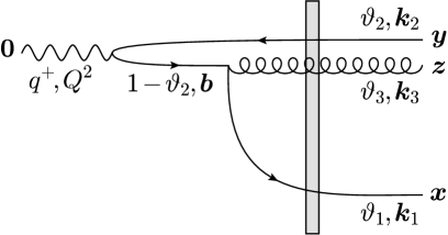
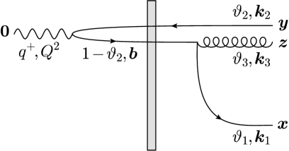
Figure 9: The probability amplitude for (2+1)-jet production in DIS off a nuclear shockwave via the channel $q^{\prime}\to q$g. The large pair is formed at the gluon vertex. Left panel: The gluon is radiated before the scattering off the shockwave. Right panel: The gluon is radiated after the scattering off the shockwave.

At this point, it is useful to remember that we are interested in special configurations which are such that the final antiquark and gluon are hard and nearly back-to-back, $k_{2\perp}\simeq k_{3\perp}\simeq P_{\perp}\gg Q_{s}(Y_{\mathbb{P}})$, whereas the final quark is semi-hard, $k_{1\perp}\sim Q_{s}(Y_{\mathbb{P}})$, and also soft, $\vartheta_{1}\ll 1$. Since the hard gluon is now emitted by the quark, this means that the intermediate quark $q^{\prime}$ must be hard as well: its transverse momentum reads $\bm{k}_{1}+\bm{k}_{3}\simeq\bm{k}_{3}$. Hence the partonic system starts as a hard quark-antiquark dipole $q^{\prime}\bar{q}$, with small transverse size $r\sim 1/P_{\perp}$, which then evolves by emitting a soft quark at some large distance $R\sim 1/k_{1\perp}$ from the other partons. This is the evolution illustrated in the left panel in Fig. 6. In so far as the distribution of colour is concerned, the intermediate $q^{\prime}\bar{q}$ pair behaves like a small dipole of size $r$, whereas the final $q\bar{q}g$ system behaves like a large quark-antiquark dipole with size $R$. Since the scattering of a small dipole, with size $r\ll 1/Q_{s}$, is power suppressed, this immediately implies that one can ignore the second configuration, where the gluon is emitted after the nuclear shockwave. Hence, we shall consider in detail only the first configuration (gluon emission before the scattering).

Returning to Eq. (91), we write the two energy denominators as

$$2q^{+}\big{(}E_{\bar{q}}+E_{\bar{q}^{\prime}}-E_{\gamma}\big{)}=\frac{k_{2\perp}^{2}}{\vartheta_{2}}+\frac{k_{2\perp}^{2}}{1-\vartheta_{2}}+Q^{2}\simeq\frac{P_{\perp}^{2}}{\vartheta_{2}\vartheta_{3}}+Q^{2}$$ (96)

and

$$2q^{+}\big{(}E_{q}+E_{\bar{q}}+E_{g}-E_{\gamma}\big{)} \,=\frac{k_{1\perp}^{2}}{\vartheta_{1}}+\frac{k_{2\perp}^{2}}{\vartheta_{2}}+\frac{k_{3\perp}^{2}}{\vartheta_{3}}+Q^{2}\simeq\frac{k_{1\perp}^{2}+\mathcal{M}^{2}}{\vartheta_{1}},$$ (97)

where $\mathcal{M}^{2}$ is the scale already defined in Eq. (79). In arriving at the last approximate equalities in Eqs. (96) and (97) we have used the fact that $k_{2\perp}\simeq k_{3\perp}\simeq P_{\perp}$ and we have assumed $\vartheta_{1}\ll 1$, hence $\vartheta_{2}+\vartheta_{3}\simeq 1$. The softness of $\vartheta_{1}$ follows from the same formation-time argument as presented in Sect. 3.1 for (2+1)–jets with a soft gluon: the formation time $\tau_{q}\sim 2\vartheta_{1}q^{+}/k_{1\perp}^{2}$ of the soft quark must be shorter than the lifetime $\tau_{q^{\prime}\bar{q}}\sim 2q^{+}/P_{\perp}^{2}$ of the intermediate dipole before its scattering with the target. This implies $\vartheta_{1}\lesssim k_{1\perp}^{2}/P_{\perp}^{2}\ll 1$, which in turn shows that the relative momentum $\bar{\bm{K}}$ of the quark-gluon pair is semi-hard, $\bar{\bm{K}}\simeq\bm{k}_{1}$, despite the fact that the final gluon is hard.

Inserting the above approximations into Eq. (91) we obtain the following expression for the amplitude corresponding to the first configuration (below, $\tilde{Q}^{2}\equiv\vartheta_{2}\vartheta_{3}Q^{2}$):

$$\Psi^{im}_{\lambda_{1}\lambda_{2}(q)}\simeq-\,\delta_{\lambda_{1}\lambda_{2}}\,\frac{ee_{f}gq^{+}}{2(2\pi)^{6}}\,\frac{1}{\vartheta_{3}^{3/2}}\,\frac{\varphi^{ij*}(\vartheta_{2},\lambda_{1})P^{j}}{P_{\perp}^{2}+\tilde{Q}^{2}}\,\frac{\tau^{mn*}(\vartheta_{2},0,\lambda_{1})k_{1}^{n}}{k_{1\perp}^{2}+\mathcal{M}^{2}},$$ (98)

Like in the previous subsection, we expect the system of the three partons to effectively scatter like a large quark-antiquark dipole. To see that, let us introduce appropriate variables in coordinate space:

$$\bm{r}\equiv\bm{y}-\bm{b},\qquad\bm{R}\equiv\bm{x}-\bm{z},\qquad\bm{b}\equiv\frac{\vartheta_{1}\bm{x}+\vartheta_{3}\bm{z}}{\vartheta_{1}+\vartheta_{3}}.$$ (99)

Here, $\bm{r}$ is the separation between the antiquark and the intermediate quark, $\bm{R}$ is the one between the final quark and the gluon and $\bm{b}$ is the position of the intermediate quark. The inverse transformation reads

$$\bm{x}=\bm{b}+\frac{\vartheta_{3}}{\vartheta_{1}+\vartheta_{3}}\,\bm{R},\qquad\bm{y}=\bm{b}+\bm{r},\qquad\bm{z}=\bm{b}-\frac{\vartheta_{1}}{\vartheta_{1}+\vartheta_{3}}\,\bm{R},$$ (100)

so that the phase involved in the Fourier transform from momentum to coordinate space becomes

$$\bm{k}_{1}\cdot\bm{x}+\bm{k}_{2}\cdot\bm{y}+\bm{k}_{3}\cdot\bm{z}\,=\,\bm{k}_{2}\cdot\bm{r}+\bar{\bm{K}}\cdot\bm{R}\,\simeq\,\bm{P}\cdot\bm{r}+\bm{k}_{1}\cdot\bm{R}.$$ (101)

The final result is like in Eq. (83), so the comments following the latter apply also here. In particular, we have $r\ll R$, that is, $q^{\prime}$ and $\bar{q}$ are very close to each other. From Eq. (100) we also find that when $\vartheta_{1}\ll k_{1\perp}/P_{\perp}\ll 1$ the emitted gluon has the same transverse position as its source. Eventually the soft final quark $q$ “sees” the two other final partons at the same transverse position: $\bm{z}\simeq\bm{y}\simeq\bm{b}$. The general structure of the scattering matrix corresponding to this configuration is again given by Eq. (85) and its projection on elastic scattering is obtained by replacing $t^{a}_{\alpha\beta}\to-\mathcal{T}(\bm{R})\,t^{a}_{\alpha\beta}$, cf. (87), in the LCWF (3.2). We can further convince ourselves that the second configuration, where the gluon is emitted at $x^{+}>0$, is proportional to $\mathcal{T}(\bm{r})$, which confirms our expectation that it is power-suppressed.

The functional dependence on $\bm{k}_{1}$ of the total wavefunction $\Psi_{(q)}$ in Eq. (98) is the same as the one we encountered when the gluon source was the antiquark, cf. (80), so we just need to do the replacement dictated by (3.2) to properly include the scattering described by $\mathcal{T}(\bm{R})$. We finally arrive at the diffractive amplitude for (2+1)-jet production via the channel $q^{\prime}\to qg$ and such that the quark jet is semi-hard (in transverse momentum) and soft (in longitudinal momentum)

$$\Psi^{im,D}_{\lambda_{1}\lambda_{2}(q)}\simeq\delta_{\lambda_{1}\lambda_{2}}\,\frac{ee_{f}gq^{+}}{2(2\pi)^{6}}\,\frac{\Phi^{ijmn}_{(q)}(\vartheta_{2},\lambda_{1})}{\vartheta_{3}^{3/2}}\,\frac{P^{j}}{P_{\perp}^{2}+\tilde{Q}^{2}}\,\frac{K_{\perp}^{n}}{K_{\perp}}\,\frac{\mathcal{Q}_{T}(\mathcal{M},K_{\perp})}{\mathcal{M}},$$ (102)

with $\vartheta_{2}+\vartheta_{3}\simeq 1$ and where we recall that $\bm{K}=\bm{k}_{2}+\bm{k}_{3}$ is the transverse momentum imbalance in the hard $\bar{q}g$ dijet. The spinorial and polarisation structure is contained in

$$\Phi^{ijmn}_{(q)}(\vartheta,\lambda)\,\equiv\,-\,\varphi^{ij*}(\vartheta,\lambda)\tau^{mn*}(\vartheta,0,\lambda)=(1-\vartheta)\big{[}(1-2\vartheta)\delta^{ij}+2i\lambda\varepsilon^{ij}\big{]}\big{[}\delta^{mn}-2i\lambda\varepsilon^{mn}\big{]}.$$ (103)

3.4 The cross section for diffractive 2+1 jets with a soft quark

The cross section for the diffractive (2+1)-jet production is determined similarly to the one for exclusive dijets in Eq. (23), i.e. by counting the number of partons in the final state with the desired longitudinal and transverse momenta. Following once more the normalizations in Iancu:2018hwa we find

$$\frac{{\rm d}\sigma^{\gamma_{\scriptscriptstyle T}^{*}A\rightarrow(q)\bar{q}gA}}{{\rm d}\vartheta_{1}{\rm d}\vartheta_{2}{\rm d}\vartheta_{3}{\rm d}^{2}\bm{k}_{1}{\rm d}^{2}\bm{k}_{2}{\rm d}^{2}\bm{k}_{3}}=\frac{(2\pi)^{6}S_{\perp}C_{F}N_{c}}{2(q^{+})^{2}}\,\delta(1\!-\!\vartheta_{1}\!-\!\vartheta_{2}\!-\!\vartheta_{3})\,\delta^{(2)}(\bm{k}_{1}+\bm{k}_{2}+\bm{k}_{3})\!\sum_{\begin{subarray}{c}i,m\\ \lambda_{1},\lambda_{2}\end{subarray}}\!\big{|}\Psi_{\lambda_{1}\lambda_{2}}^{im,\,D}\big{|}^{2},$$ (104)

where the overall colour factor emerged as ${\rm tr}[t^{a}t^{a}]=C_{F}N_{c}$. In writing the final state, the quark label is shown in parentheses, “$(q)$”, to emphasise that this is the soft parton from the (2+1)–jet. The wavefunction $\Psi_{\lambda_{1}\lambda_{2}}^{im,D}$ in the above is simply the sum of the expressions in Eqs. (89) and Eqs. (102), which were obtained for gluon emission from the antiquark and the quark respectively. By using the $\delta$-function to perform one of the two-dimensional integrations and switching to the $\bm{P}$ and $\bm{K}$ variables we trivially get

$$\frac{{\rm d}\sigma^{\gamma_{\scriptscriptstyle T}^{*}A\rightarrow(q)\bar{q}gA}}{{\rm d}\vartheta_{1}{\rm d}\vartheta_{2}{\rm d}\vartheta_{3}{\rm d}^{2}\bm{P}{\rm d}^{2}\bm{K}}=\frac{(2\pi)^{6}S_{\perp}C_{F}N_{c}}{2(q^{+})^{2}}\,\delta_{\vartheta}\!\sum_{\begin{subarray}{c}i,m\\ \lambda_{1},\lambda_{2}\end{subarray}}\!\left\{\big{|}\Psi_{\lambda_{1}\lambda_{2}(\bar{q})}^{im,D}\big{|}^{2}\!+\!\big{|}\Psi_{\lambda_{1}\lambda_{2}(q)}^{im,D}\big{|}^{2}\!+\!2\Re\!\left[\Psi_{\lambda_{1}\lambda_{2}(\bar{q})}^{im,D}\Psi_{\lambda_{1}\lambda_{2}(q)}^{im,D*}\right]\right\}\!,$$ (105)

where for the economy of the notation we defined $\delta_{\vartheta}\equiv\delta(1-\vartheta_{1}-\vartheta_{2}-\vartheta_{3})\simeq\delta(1-\vartheta_{2}-\vartheta_{3})$. In what follows, we shall separately compute the three contributions to the cross section.

(i) Direct term from gluon emission by the antiquark.

Let us consider the first term in Eq. (105). Starting with Eq. (90), it is an easy exercise to find (recall that $\lambda^{2}=1/4$)

$$\sum_{i,m,\lambda}\Phi^{ijmn}_{(\bar{q})}(\vartheta,\lambda)\Phi^{ikmr*}_{(\bar{q})}(\vartheta,\lambda)=8(1+\vartheta^{2})\delta^{jk}\delta^{nr}+8(1-\vartheta^{2})\varepsilon^{jk}\varepsilon^{nr}.$$ (106)

Notice that when we calculate $\big{|}\Psi_{(\bar{q})}^{D}\big{|}^{2}$, we encounter the momenta tensorial structure $K^{j}K^{k}P^{n}P^{r}$ and the second, antisymmetric, term in Eq. (106) does not contribute. Substituting into Eq. (105) we obtain for this part of the cross section in which the gluon is emitted by the antiquark both in the DA and in the CCA

$$\frac{{\rm d}\sigma_{(\bar{q}\bar{q})}^{\gamma_{\scriptscriptstyle T}^{*}A\rightarrow(q)\bar{q}gA}}{{\rm d}\vartheta_{1}{\rm d}\vartheta_{2}{\rm d}\vartheta_{3}\,{\rm d}^{2}\bm{P}{\rm d}^{2}\bm{K}}=\frac{S_{\perp}\alpha_{\rm em}N_{c}}{2\pi^{4}}\left(\sum e_{f}^{2}\right)\delta_{\vartheta}\,\frac{\alpha_{s}C_{F}}{P_{\perp}^{2}}\frac{1+(1-\vartheta_{3})^{2}}{2\vartheta_{3}}\,\frac{\big{|}\mathcal{Q}_{T}(\mathcal{M},K_{\perp},Y_{\mathbb{P}})\big{|}^{2}}{\mathcal{M}^{2}},$$ (107)

with $\alpha_{s}=g^{2}/4\pi$ the strong coupling constant and $\mathcal{M}^{2}$ as defined in Eq. (79). One recognises here the DGLAP splitting function

$$P_{gq}(\vartheta_{3})=C_{F}\frac{1+(1-\vartheta_{3})^{2}}{\vartheta_{3}}\,$$ (108)

and the characteristic transverse momentum spectrum $1/P_{\perp}^{2}$ for a hard splitting $\bar{q}^{\prime}\to\bar{q}g$ occurring in the final state.

(ii) Direct term from gluon emission by the quark.

Now we move on to the second term in Eq. (105). Starting with Eq. (103), we get

$$\sum_{i,m,\lambda}\Phi^{ijmn}_{(q)}(\vartheta,\lambda)\Phi^{ikmr*}_{(q)}(\vartheta,\lambda)=8(1-\vartheta)^{2}\left\{\left[\vartheta^{2}+(1-\vartheta)^{2}\right]\delta^{jk}\delta^{nr}+(1-2\vartheta)\varepsilon^{jk}\varepsilon^{nr}\right\}.$$ (109)

When we calculate $\big{|}\Psi_{(q)}^{D}\big{|}^{2}$, we encounter the structure $P^{j}P^{k}K^{n}K^{r}$, so that again the antisymmetric term in Eq. (109) does not contribute. Substituting into Eq. (105) we obtain for this part of the cross section in which the gluon is emitted by the quark in both the DA and the CCA (with $\tilde{Q}^{2}\equiv\vartheta_{2}\vartheta_{3}Q^{2}$)

$$\frac{{\rm d}\sigma_{(qq)}^{\gamma_{\scriptscriptstyle T}^{*}A\rightarrow(q)\bar{q}gA}}{{\rm d}\vartheta_{1}{\rm d}\vartheta_{2}{\rm d}\vartheta_{3}\,{\rm d}^{2}\bm{P}{\rm d}^{2}\bm{K}}=\frac{S_{\perp}\alpha_{\rm em}N_{c}}{2\pi^{4}}\left(\sum e_{f}^{2}\right)\delta_{\vartheta}\,\frac{\alpha_{s}C_{F}P_{\perp}^{2}}{(P_{\perp}^{2}+\tilde{Q}^{2})^{2}}\frac{\vartheta_{2}^{2}+(1-\vartheta_{2})^{2}}{2\vartheta_{3}}\,\frac{\big{|}\mathcal{Q}_{T}(\mathcal{M},K_{\perp},Y_{\mathbb{P}})\big{|}^{2}}{\mathcal{M}^{2}}.$$ (110)

(iii) Interference term.

Finally we go to the last, interference, term in Eq. (105). Using Eqs. (90) and (103), we obtain

$$\sum_{i,m,\lambda}\Phi^{ijmn}_{(\bar{q})}(\vartheta,\lambda)\Phi^{ikmr*}_{(q)}(\vartheta,\lambda)=-8\vartheta^{2}(1-\vartheta)(\delta^{jk}\delta^{nr}-\varepsilon^{jk}\varepsilon^{nr}).$$ (111)

In the wavefunction $\Psi_{(\bar{q})}^{D}$ the semi-hard momentum $\bm{K}$ is attached to the photon vertex and the hard momentum $\bm{P}$ in the gluon vertex, while in $\Psi_{(q)}^{D}$ the opposite happens. This is just a consequence of the fact that the large dipole is created directly at the photon vertex in the former case and in the gluon vertex in the latter. Hence, when we calculate the cross product $\Psi_{(\bar{q})}^{D}\Psi_{(q)}^{D*}$, we meet a substantially different tensorial structure in the momentum sector, namely $K^{j}P^{k}P^{n}K^{r}$. As a result the term involving the antisymmetric symbols is now relevant and we have

$$(\delta^{jk}\delta^{nr}-\varepsilon^{jk}\varepsilon^{nr})K^{j}P^{k}P^{n}K^{r}=(\bm{P}\cdot\bm{K})^{2}+(\bm{P}\times\bm{K})^{2}=P_{\perp}^{2}K_{\perp}^{2},$$ (112)

so that the dependence on the two momenta factorizes. Remarkably, the particular combination of the two terms in Eq. (112) eliminates any potential angular correlation between the hard and semi-hard momenta.

Putting everything together and substituting into Eq. (105) we obtain the interference contribution to the cross section in the form

$$\frac{{\rm d}\sigma_{(\bar{q}q)}^{\gamma_{\scriptscriptstyle T}^{*}A\rightarrow(q)\bar{q}gA}}{{\rm d}\vartheta_{1}{\rm d}\vartheta_{2}{\rm d}\vartheta_{3}\,{\rm d}^{2}\bm{P}{\rm d}^{2}\bm{K}}=-\frac{S_{\perp}\alpha_{\rm em}N_{c}}{2\pi^{4}}\left(\sum e_{f}^{2}\right)\delta_{\vartheta}\,\frac{\alpha_{s}C_{F}}{P_{\perp}^{2}+\tilde{Q}^{2}}\,\frac{\vartheta_{2}^{2}}{\vartheta_{3}}\,\frac{\big{|}\mathcal{Q}_{T}(\mathcal{M},K_{\perp},Y_{\mathbb{P}})\big{|}^{2}}{\mathcal{M}^{2}}.$$ (113)

This is negative, as typically expected for an interference term.

4 TMD factorisation for diffractive (2+1)–jets with a soft quark

So far, the cross-section for diffractive (2+1)–jet production with a soft quark has been constructed by working in the colour dipole picture, where the parton evolution is exclusively associated with the projectile: the three partons appearing in the final state have all been generated via radiation in the wavefunction of the virtual photon. In what follows, we would like to show that, after a suitable change of variables, the result can be reinterpreted in terms of target evolution: the soft quark can alternatively be viewed as a constituent of the Pomeron. The partonic picture of the Pomeron is exactly the same as discussed in Sect. 2, in relation with diffractive SIDIS (i.e. exclusive dijets in the aligned jet configuration). The Pomeron fluctuates into a semi-hard quark-antiquark pair: an on-shell quark in the $s$–channel (which appears in the final state) and a space-like antiquark in the $t$–channel (which interacts with the projectile). The differences between exclusive dijets and (2+1)–jets with a soft quark refer to final state interactions, as we now explain.

From Sect. 2, we recall that in diffractive SIDIS the $t$–channel antiquark gets on-shell after absorbing the virtual photon and appears in the final state (see the right panel in Fig. 3). For the (2+1)–jet process depicted in the right panel in Fig. 6 (gluon emission by the antiquark), the antiquark remains virtual after absorbing the photon and eventually decays into a hard $\bar{q}g$ pair, which appears in the final state. This interpretation is illustrated in the left diagram in Fig. 10, which looks like the SIDIS graph in the right panel in Fig. 3, but with an additional gluon emission in the final state. For the other (2+1)–jet process, where the gluon is emitted by the quark, cf. the left panel in Fig. 6, the $t$–channel antiquark does not directly couple to the virtual photon, rather it annihilates against the ($s$–channel) quark from the hard $q\bar{q}$ dipole generated by the photon decay. This annihilation process, which gives rise to a hard gluon in the final state, is illustrated in the right diagram in Fig. 10. By combining the two pictures above, one deduces a graphical representation for the interference contribution to the (2+1)–jet cross-section, shown as the bottom diagram in Fig. 10.

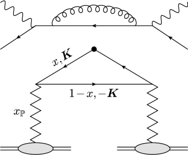
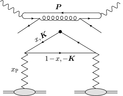
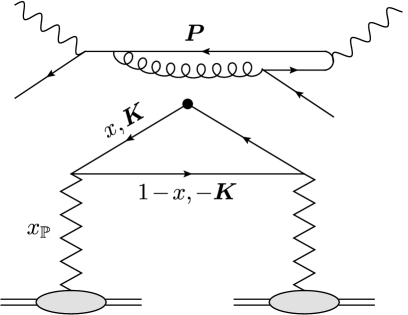
Figure 10: TMD factorization in forward dijet production in DIS off a nucleus. The soft quark from the dipole picture is now viewed as a constituent of the target wavefunction. The Pomeron splits into a quark-antiquark dipole: an $s$–channel quark with longitudinal fraction $1-x$, which appears in the final state, and a $t$–channel antiquark with longitudinal fraction $x$, which participates in the scattering with the virtual photon. Left panel: The $t$–channel antiquark first absorbs the photon and then splits into a hard antiquark-gluon pair. Right panel: The $t$–channel antiquark annihilates against the quark from a hard quark-antiquark fluctuation of the photon. Bottom panel: An interference contribution.

The physical picture that we just described is suggestive of TMD factorisation, with the same quark diffractive TMD as introduced in Sect. 2. This is furthermore supported by the fact that all three contributions to the cross-section — the direct gluon emissions in Eqs. (107) and (110), and the interference contribution in Eq. (113) — are proportional to $|\mathcal{Q}_{T}|^{2}$, which is the main ingredient of the quark DTMD (recall Eqs. (32)–(34)). But in order to make the TMD factorisation manifest, one still needs to perform a change of longitudinal variables, from the projectile-oriented variable $\vartheta_{1}$ (the “plus” longitudinal momentum fraction of the final quark w.r.t. the virtual photon) to the target-oriented variable $x$ (the “minus” longitudinal fraction of the $t$–channel antiquark w.r.t. the Pomeron). To that aim, one can use the same argument as in Sect. 2.4, that is, the condition that the $s$–channel quark with “minus” longitudinal fraction $1-x$ be on-shell, cf. Eq. (37).

Alternatively, and perhaps more instructive for the present purposes, one can use the conservation of the minus longitudinal momentum: the momentum $xx_{\mathbb{P}}P_{N}^{-}$ carried by the $t$–channel virtual quark gets transmitted to the “hard” part of the amplitude, hence it must compensate the (negative) LC energy of the virtual photon, $q^{-}=-Q^{2}/2q^{+}$, and put the final $\bar{q}g$ pair on shell. This argument implies $xx_{\mathbb{P}}=x_{\bar{q}g}$, with

$$x_{\bar{q}g}\equiv\frac{1}{2q^{+}P_{N}^{-}}\left(\frac{k^{2}_{2\perp}}{\vartheta_{2}}+\frac{k^{2}_{3\perp}}{\vartheta_{3}}+Q^{2}\right)=\frac{1}{\hat{s}}\left(\frac{\vartheta_{2}+\vartheta_{3}}{\vartheta_{2}\vartheta_{3}}\,P_{\perp}^{2}+\frac{K_{\perp}^{2}}{\vartheta_{2}+\vartheta_{3}}+Q^{2}\right)\simeq\frac{1}{\hat{s}}\left(\frac{P_{\perp}^{2}}{\vartheta_{2}\vartheta_{3}}+Q^{2}\right)\,,$$ (114)

where we have also used the conditions $\vartheta_{1}\ll 1$ and $K_{\perp}^{2}\ll P_{\perp}^{2},\,Q^{2}$ to simplify the result. Similarly,

$$x_{\mathbb{P}}=\frac{1}{2q^{+}P_{N}^{-}}\left(\frac{k_{1\perp}^{2}}{\vartheta_{1}}+\frac{k_{2\perp}^{2}}{\vartheta_{2}}+\frac{k_{3\perp}^{2}}{\vartheta_{3}}+Q^{2}\right)\simeq\frac{1}{\hat{s}}\left(\frac{P_{\perp}^{2}}{\vartheta_{2}\vartheta_{3}}+Q^{2}+\frac{K_{\perp}^{2}}{\vartheta_{1}}\right)\,.$$ (115)

Using these results together with $x=x_{\bar{q}g}/x_{\mathbb{P}}$, one finds the following relation between $\vartheta_{1}$ and $x$,

$$\vartheta_{1}=\frac{x}{1-x}\,\frac{K_{\perp}^{2}}{\frac{P_{\perp}^{2}}{\vartheta_{2}\vartheta_{3}}+{Q}^{2}},$$ (116)

which we recall is only valid so long as the $\vartheta_{1}\ll 1$ (the produced quark must be soft w.r.t. the projectile in order to be reinterpreted as a constituent of the target). The r.h.s. of Eq. (116) is indeed much smaller than one in the transverse kinematics of interest ($K_{\perp}\ll P_{\perp}$) and for generic values of $x$. Vice-versa, our approximations fail when $1-x$ is so small that the r.h.s. of Eq. (116) becomes of order one.

Using Eq. (116), one can now finalise our change of variables and thus demonstrate TMD factorisation. Recalling the definition (79) of the quantity $\mathcal{M}^{2}$, one can use (116) to express this quantity in terms of the target variables $x$ and $K_{\perp}$, as required by factorisation:

$$\mathcal{M}^{2}=\frac{x}{1-x}\,K_{\perp}^{2}\,.$$ (117)

One also needs to change the measure in the differential cross-sections; this is done by using

$$\frac{{\rm d}\vartheta_{1}}{\vartheta_{1}}=\frac{1}{1-x}\,\frac{{\rm d}x}{x}\,.$$ (118)

Omitting unnecessary variables, it is easy to see that the differential cross-section per unit $x$ can be obtained as

$$x\frac{{\rm d}\sigma}{{\rm d}x}\,=\,\frac{\vartheta_{1}}{1-x}\,\frac{{\rm d}\sigma}{{\rm d}\vartheta_{1}}\,=\,\frac{x}{(1-x)^{2}}\,\frac{\vartheta_{2}\vartheta_{3}K_{\perp}^{2}}{P_{\perp}^{2}+\tilde{Q}^{2}}\,\frac{{\rm d}\sigma}{{\rm d}\vartheta_{1}}\,,$$ (119)

where we recall the notation $\tilde{Q}^{2}\equiv\vartheta_{2}\vartheta_{3}Q^{2}$.

To summarise, the new independent variables are the kinematical variables $\vartheta_{2}$, $\vartheta_{3}$ and $\bm{P}$ of the hard dijets together with the target variables $x$ and $\bm{K}$ (besides the general DIS variables $Q^{2}$ and $x_{\rm\scriptscriptstyle Bj}$). We recall that $\bm{K}$ has several meanings (by virtue of transverse momentum conservation): it represents the transverse momentum of the virtual antiquark exchanged in the $t$–channel, but also minus the transverse momentum of the final quark ($\bm{k}_{1}=-\bm{K}$) and, finally, the transverse momentum imbalance between the hard dijets ($\bm{K}=\bm{k}_{2}+\bm{k}_{3}$). Notice also that the more standard diffractive variables $x_{\mathbb{P}}$ and $\beta$ are not independent variables, rather they can be expressed as

$$x_{\mathbb{P}}=\frac{x_{\bar{q}g}}{x}=\frac{x_{\rm\scriptscriptstyle Bj}}{x}\,\frac{P_{\perp}^{2}+\tilde{Q}^{2}}{\tilde{Q}^{2}}\,,\qquad\beta=\frac{x_{\rm\scriptscriptstyle Bj}}{x_{\mathbb{P}}}=x\,\frac{\tilde{Q}^{2}}{P_{\perp}^{2}+\tilde{Q}^{2}}\,.$$ (120)

In practice, one can use any of the three variables $x$, $x_{\mathbb{P}}$ and $\beta$ as the independent “target longitudinal momentum variable” and then use Eq. (120) to express the two others. In this section, we shall write the cross-section per unit of $\ln(1/x)$, but in Sect. 3.1 we have chosen $Y_{\mathbb{P}}=\ln(1/x_{\mathbb{P}})$ as the independent variable (recall Eq. (59)) and in the next section we shall find it more convenient to work with $\ln(1/\beta)$.

We are now prepared to rewrite the cross-section for diffractive (2+1)–jets with a soft quark in terms of the new variables and thus demonstrate TMD factorisation. We shall separately consider the three contributions to the cross-section isolated in Sect. 3.4.

(i) Direct term from gluon emission by the antiquark.

Making the aforementioned change of variables, cf. Eqs. (116)–(119), we can put Eq. (107) in the manifestly factorised form

$$\frac{{\rm d}\sigma_{(\bar{q}\bar{q})}^{\gamma_{\scriptscriptstyle T}^{*}A\rightarrow(q)\bar{q}gA}}{{\rm d}\vartheta_{2}{\rm d}\vartheta_{3}{\rm d}^{2}\bm{P}{\rm d}^{2}\bm{K}\,{\rm d}\ln(1/x)}=\frac{4\pi^{2}\alpha_{\rm em}}{Q^{2}}\,\left(\sum e_{f}^{2}\right)\,\mathcal{H}_{T}^{(\bar{q}\bar{q})}(\vartheta_{2},\vartheta_{3},P_{\perp}^{2},\tilde{Q}^{2})\,\frac{{\rm d}xq_{\mathbb{P}}(x,x_{\mathbb{P}},K_{\perp}^{2})}{{\rm d}^{2}\bm{K}}.$$ (121)

This expression exhibits a double factorisation: it is the product of two hard factors and a semi-hard one (see the left panel in Fig. 10). The first hard factor describes the absorption of the virtual photon by a semi-hard antiquark from the target; this process is “hard” when $Q^{2}$ is large. The second hard factor, defined as (from now on, it is understood that $\delta_{\vartheta}=\delta(1-\vartheta_{2}-\vartheta_{3})$)

$$\mathcal{H}^{(\bar{q}\bar{q})}_{T}(\vartheta_{2},\vartheta_{3},P_{\perp}^{2},\tilde{Q}^{2})\equiv\delta_{\vartheta}\,\frac{\alpha_{s}}{2\pi^{2}}\,P_{gq}(\vartheta_{3})\,\frac{\tilde{Q}^{2}}{P^{2}_{\perp}(P_{\perp}^{2}+\tilde{Q}^{2})},$$ (122)

describes the decay of the intermediate antiquark $\bar{q}^{\prime}$ into a hard antiquark-gluon pair $\bar{q}g$ (indeed, it features the DGLAP splitting function $P_{gq}(\vartheta_{3})$ which was introduced in Eq. (108)). Being hard, this decay fully factorises from the remaining part of the process, which describes the formation of the initial $q\bar{q}$ pair and admits TMD factorisation for the reasons explained in Sect. 2. And indeed, the last (“semi-hard”) factor in Eq. (121) is the quark TMD already introduced in Eq. (34).

Although natural at high $Q^{2}$, the double factorisation in Eq. (121) somehow obscures that fact that this cross-section applies for any value of $Q^{2}$ and in particular it remains finite in the photo-production limit $Q^{2}\to 0$ (as relevant e.g. for UPCs). Indeed, the inverse power $1/Q^{2}$ from the first hard factor cancels against the overall power $\tilde{Q}^{2}=\vartheta_{2}\vartheta_{3}Q^{2}$ from the second hard factor.

(ii) Direct term from gluon emission by the quark.

For this process too, one can rewrite the cross-section (110) in a form which looks similar to Eq. (121), namely

$$\frac{{\rm d}\sigma_{(qq)}^{\gamma_{\scriptscriptstyle T}^{*}A\rightarrow(q)\bar{q}gA}}{{\rm d}\vartheta_{2}{\rm d}\vartheta_{3}{\rm d}^{2}\bm{P}{\rm d}^{2}\bm{K}\,{\rm d}\ln(1/x)}=\frac{4\pi^{2}\alpha_{\rm em}}{Q^{2}}\left(\sum e_{f}^{2}\right)\mathcal{H}_{T}^{(qq)}(\vartheta_{2},\vartheta_{3},P_{\perp}^{2},\tilde{Q}^{2})\,\frac{{\rm d}xq_{\mathbb{P}}(x,x_{\mathbb{P}},K_{\perp}^{2})}{{\rm d}^{2}\bm{K}},$$ (123)

where the second hard factor reads

$$\mathcal{H}_{T}^{(qq)}(\vartheta_{2},\vartheta_{3},P_{\perp}^{2},\tilde{Q}^{2})\equiv\delta_{\vartheta}\,\frac{\alpha_{s}C_{F}}{\pi^{2}}\,P_{q\gamma}(\vartheta_{2})\,\frac{1}{\vartheta_{3}}\,\frac{\tilde{Q}^{2}P^{2}_{\perp}}{(P_{\perp}^{2}+\tilde{Q}^{2})^{3}}\quad\mathrm{with}\quad P_{q\gamma}(\vartheta_{2})=\frac{1}{2}\left[\vartheta_{2}^{2}+(1-\vartheta_{2})^{2}\right].$$ (124)

In this case, however, the writing in Eq. (123) must be taken with a grain of salt: despite this writing, this process does not admit a genuine “double factorisation”. Its hard part includes two elementary processes — the photon decay into a hard $q\bar{q}$ pair and the annihilation of the ($s$–channel) quark from this pair against the ($t$–channel) antiquark from the Pomeron — which strictly speaking do not factorise from each other. Rather, they are together described by the product of the two “hard factors” in the r.h.s. of Eq. (123), which physically cannot be separated from each other. For instance, the second factor $\mathcal{H}_{T}^{(qq)}$ describes both the photon decay $\gamma\to q\bar{q}$ (as obvious from the presence of the electromagnetic splitting function $P_{q\gamma}(\vartheta_{2})$) and the subsequent gluon emission $q^{\prime}\to qg$ (the “annihilation process”). The overall process is illustrated by the second diagram in Fig. 10.

It is perhaps useful to recall the origin of the factor $1/\vartheta_{3}$ in Eq. (124): unlike in Eq. (122), this factor has not been generated by the gluon emission. Indeed, the splitting fraction of the gluon at the $q^{\prime}\to qg$ vertex is $\vartheta_{3}/(\vartheta_{1}+\vartheta_{3})\simeq 1$, so the respective splitting function becomes trivial. Rather, by inspection of the calculation in Sect. 3.3, one sees that this factor has been generated as $1/\vartheta_{1}^{\prime}\simeq 1/\vartheta_{3}$, where $\vartheta_{1}^{\prime}\equiv\vartheta_{1}+\vartheta_{3}$ is the longitudinal fraction of the intermediate quark state, prior to the gluon emission. In turn, this factor $1/\vartheta_{1}^{\prime}$ comes from the normalisation of the respective single-particle state.

(iii) Interference term.

Finally, the contribution to the cross section from the interference term, cf. Eq. (113), becomes

$$\frac{{\rm d}\sigma_{(\bar{q}q)}^{\gamma_{\scriptscriptstyle T}^{*}A\rightarrow(q)\bar{q}gA}}{{\rm d}\vartheta_{2}{\rm d}\vartheta_{3}{\rm d}^{2}\bm{P}{\rm d}^{2}\bm{K}\,{\rm d}\ln(1/x)}=-\frac{4\pi^{2}\alpha_{\rm em}}{Q^{2}}\left(\sum e_{f}^{2}\right)\delta_{\vartheta}\,\frac{\alpha_{s}C_{F}}{\pi^{2}}\,\frac{\vartheta_{2}^{2}}{\vartheta_{3}}\,\frac{\tilde{Q}^{2}}{(P_{\perp}^{2}+\tilde{Q}^{2})^{2}}\,\frac{{\rm d}xq_{\mathbb{P}}(x,x_{\mathbb{P}},K_{\perp}^{2})}{{\rm d}^{2}\bm{K}},$$ (125)

and is illustrated by the lower graph in Fig. 10.

(iv) Total cross-section in the transverse sector.

Putting together the three contributions in Eqs. (121), (123) and (125) we arrive at the total cross section for (2+1)-jet diffractive production for the case of an initial photon with transverse polarisation. It reads

$$\frac{{\rm d}\sigma^{\gamma_{\scriptscriptstyle T}^{*}A\rightarrow(q)\bar{q}gA}}{{\rm d}\vartheta_{2}{\rm d}\vartheta_{3}{\rm d}^{2}\bm{P}{\rm d}^{2}\bm{K}\,{\rm d}\ln(1/x)}=\frac{4\pi^{2}\alpha_{\rm em}}{Q^{2}}\left(\sum e_{f}^{2}\right)\mathcal{H}_{T}(\vartheta_{2},\vartheta_{3},P_{\perp}^{2},\tilde{Q}^{2})\,\frac{{\rm d}xq_{\mathbb{P}}(x,x_{\mathbb{P}},K_{\perp}^{2})}{{\rm d}^{2}\bm{K}},$$ (126)

where the combined hard factor acquires the relatively simple form

$$\mathcal{H}_{T}(\vartheta_{2},\vartheta_{3},P_{\perp}^{2},\tilde{Q}^{2})=\delta_{\vartheta}\,\frac{\alpha_{s}C_{F}}{\pi^{2}}\,\frac{1}{2\vartheta_{3}}\,\frac{\tilde{Q}^{2}\big{[}(P_{\perp}^{2}+\tilde{Q}^{2})^{2}+\vartheta_{2}^{2}\tilde{Q}^{4}+\vartheta_{3}^{2}P_{\perp}^{4}\big{]}}{P_{\perp}^{2}(P_{\perp}^{2}+\tilde{Q}^{2})^{3}}.$$ (127)

This cross section remains finite in the photo-production limit $Q^{2}\to 0$, hence the above results are also relevant for applications to UPCs. At large $P_{\perp}$ (by which we mean either $P_{\perp}^{2}\gg\tilde{Q}^{2},\,Q_{s}^{2}$, or $P_{\perp}^{2}\sim\tilde{Q}^{2}\gg Q_{s}^{2}$), the cross-section decreases like $1/P_{\perp}^{4}$, which is much slower than the $1/P_{\perp}^{6}$ decay of the cross-section for exclusive dijets (cf. the discussion in Appendix B). This confirms our main argument, that the diffractive production of hard dijets is controlled by (formally, next-to-leading order) processes involving 2+1 jets.

(v) The longitudinal sector.

For the case of a virtual photon with longitudinal polarisation, the calculations of the $q\bar{q}g$ component of the photon LCWF and of the cross-section for the diffractive (2+1)-jets with a soft quark are briefly presented in Appendix A. The main difference refers to the splitting function for the decay $\gamma^{*}_{L}\to q\bar{q}$ of the longitudinal photon, which reads

$$P_{q\gamma}^{L}(\vartheta)\,=\,4\vartheta(1-\vartheta).$$ (128)

This is suppressed for aligned-jet configurations and, vice-versa, it favours relatively symmetric splittings with $\vartheta(1-\vartheta)\sim 1/4$. Clearly, this has important consequences for the systematics of diffractive jet production and for its twist expansion.

Among the two amplitudes contributing to (2+1)-jet production with a soft quark ($\vartheta_{1}\ll 1$), it should be clear that it is only one of them — that where the initial $q\bar{q}$ dipole is hard and the gluon is emitted by the quark, cf. Fig. 9 — which contributes at leading twist. The direct cross-section associated to this amplitude (the right diagram in Fig. 10) involves the photon splitting function $P_{q\gamma}^{L}(\vartheta_{2})\simeq 4\vartheta_{2}\vartheta_{3}$, which is of order one when the hard final dijets are quasi-symmetric. The other amplitude, which starts with a semi-hard $q\bar{q}$ dipole, cf. Fig. 8, leads to a cross-section involving the splitting function $P_{q\gamma}^{L}(\vartheta_{1})$, which is suppressed by a factor $\vartheta_{1}\sim K_{\perp}^{2}/Q^{2}\sim Q_{s}^{2}/Q^{2}\ll 1$ w.r.t. to the respective contribution (121) of the transverse sector (see Eq. (188) for an explicit result). Clearly, this implies a corresponding suppression for the interference term.

To summarise, the dominant contribution to the cross-section for (2+1)–jets in this case comes from the second diagram in Fig. 10 (gluon emission by the quark) and reads (cf. Eq. (192))

$$\frac{{\rm d}\sigma^{\gamma_{\scriptscriptstyle L}^{*}A\rightarrow(q)\bar{q}gA}}{{\rm d}\vartheta_{2}{\rm d}\vartheta_{3}{\rm d}^{2}\bm{P}{\rm d}^{2}\bm{K}\,{\rm d}\ln(1/x)}=\frac{4\pi^{2}\alpha_{\rm em}}{Q^{2}}\,\left(\sum e_{f}^{2}\right)\mathcal{H}_{L}(\vartheta_{2},\vartheta_{3},P_{\perp}^{2},\tilde{Q}^{2})\,\frac{{\rm d}xq_{\mathbb{P}}(x,x_{\mathbb{P}},K_{\perp}^{2})}{{\rm d}^{2}\bm{K}},$$ (129)

with the following hard factor (compare to Eq. (124))

$$\mathcal{H}_{L}(\vartheta_{2},\vartheta_{3},P_{\perp}^{2},\tilde{Q}^{2})\equiv\delta_{\vartheta}\,\frac{\alpha_{s}C_{F}}{\pi^{2}}\,P^{L}_{q\gamma}(\vartheta_{2})\,\frac{1}{2\vartheta_{3}}\,\frac{\tilde{Q}^{4}}{(P_{\perp}^{2}+\tilde{Q}^{2})^{3}}\,,$$ (130)

which describes the decay $\gamma^{*}_{L}\to q\bar{q}$ of the longitudinal photon followed by the annihilation of the quark against the antiquark coming from the Pomeron. So long as $\vartheta_{2}(1-\vartheta_{2})\sim 1/4$ and $Q^{2}$ is sufficiently hard, $Q^{2}\sim P_{\perp}^{2}$, this contribution is comparable to that from the transverse photon in Eq. (123). On the other hand, the longitudinal contribution vanishes, as expected, in the limit $Q^{2}\to 0$ where the photon becomes quasi-real.

The quark diffractive PDF: towards the DGLAP evolution.

So far, we have focused on exclusive final states which, besides the hard dijet (a gluon and an antiquark), also involves a semi-hard third jet (a quark). The kinematics of the three final partons was fully specified. Although formally correct to leading order accuracy in pQCD, such a precise characterisation of the final state introduces strong constraints on the higher order corrections, which can amplify the strength of the latter. Indeed, when $P_{\perp}\gg k_{3\perp}\sim Q_{s}(Y_{\mathbb{P}})$, there is a large probability $\sim\alpha_{s}\ln(P_{\perp}^{2}/Q_{s}^{2})$ for additional radiation, either in the $t$–channel exchange between the hard dijets and the Pomeron, or from the two hard jets produced in the final state. This radiation naturally leads to a broadening of the dijet distribution in their imbalance $K_{\perp}$, allowing for $K_{\perp}$–values much larger than $Q_{s}$ (logarithmically distributed within the interval $Q_{s}^{2}\ll K_{\perp}^{2}\ll P_{\perp}^{2}$). Vice-versa, the fact of imposing a relatively small value $K_{\perp}\sim Q_{s}$ for this imbalance, introduces a veto on the additional radiation, which penalises the cross-section via the “Sudakov effect” — a strong reduction in the cross-section due to the mismatch between “real” and “virtual” radiative corrections (see e.g. the discussion in Mueller:2013wwa ). Although formally of higher order in $\alpha_{s}$, the Sudakov corrections are numerically large, since enhanced by the double logarithm $\ln^{2}(P_{\perp}^{2}/Q_{s}^{2})$, and could significantly modify our leading-order estimates.

Such complications can be avoided by giving up the measurement of the hard dijet imbalance $K_{\perp}$, hence of the detailed structure of the final state. This allows for more general (less constrained) final states, which, besides the hard dijets, can involve additional radiation (one semi-hard jet, at least) with transverse momenta $k_{\perp}\ll P_{\perp}$. The cross-section for such a more inclusive process is obtained by integrating the previous results in this section over $K_{\perp}$ up to a hard scale of order $P_{\perp}$. This amounts to replacing the quark diffractive TMD with the corresponding PDF in all the previous formulae. E.g. the cross-section for the diffractive production of two hard jets accompanied by at least one soft quark is computed as (cf. Eq. (126))

$$\frac{{\rm d}\sigma^{\gamma_{\scriptscriptstyle T}^{*}A\rightarrow(q)\bar{q}gA}}{{\rm d}\vartheta_{2}{\rm d}\vartheta_{3}{\rm d}^{2}\bm{P}{\rm d}\ln(1/x)}=\frac{4\pi^{2}\alpha_{\rm em}}{Q^{2}}\left(\sum e_{f}^{2}\right)\mathcal{H}_{T}(\vartheta_{2},\vartheta_{3},P_{\perp}^{2},\tilde{Q}^{2})\,xq_{\mathbb{P}}\left(x,x_{\mathbb{P}},(1-x)P_{\perp}^{2}\right),$$ (131)

with the quark DPDF as defined in Eq. (54). This is the analog of Eq. (66) for diffractive dijets accompanied by (at least) one soft gluon.

The resolution scale $(1-x)P_{\perp}^{2}$ for the quark DPDF has been introduced by the upper limit on the integral over $K_{\perp}^{2}$ and can be understood in several ways: (i) as the condition that the size $r\sim 1/P_{\perp}$ of the hard dijet be much smaller than the (maximal) size $R_{\rm max}\sim\sqrt{1-x}/K_{\perp}$ of the effective $q\bar{q}$ dipole (cf. Eq. (47)), or (ii) as the condition that the virtuality (38) of the $t$-channel quark exchanged between the Pomeron and the hard dijets be much smaller than the transverse momentum of the latter.

From the experience with the collinear factorisation, we know that the integral over $K_{\perp}$ ensures the cancellation of the Sudakov double logs between real and virtual corrections, but it leaves behind the single logarithmic corrections describing the DGLAP evolution of the quark diffractive PDF. Clearly, it would be instructive to explicitly observe the emergence of the DGLAP evolution also in the framework of the colour dipole picture. This would represent an important additional argument in favour of the mutual consistency between the two approaches. This will be discussed in the next section.

5 (2+1)–jet contributions to diffractive SIDIS: the emergence of DGLAP

To unveil the DGLAP evolution from the colour dipole picture for (2+1)–jet production, it is convenient to consider their contributions to more inclusive quantities, like diffractive SIDIS and the diffractive structure function $F_{2}^{D(3)}(x_{\rm\scriptscriptstyle Bj},x_{\mathbb{P}},Q^{2})$. By “diffractive SIDIS” in the context of (2+1)-jets, we mean that only one of the two hard jets — a priori, either one of them — is measured in the final state. Without loss of generality, we can denote the transverse momentum of the measured jet by $\bm{P}$; then the other jet will have a momentum $-\bm{P}+\bm{K}$ and the SIDIS cross-section is obtained by integrating over all the kinematical variables that are not measured. For instance, for (2+1)-jets with a soft quark and for a virtual photon with transverse polarisation, the original cross-section (126) must be integrated over $\vartheta_{2},\,\vartheta_{3}$, $\bm{K}$, and $x$ at a fixed value of the rapidity gap $Y_{\mathbb{P}}$ — or, equivalently, of the diffractive variable $\beta$. In what follows, we choose to work with $\beta$, that is, we shall construct the analog of Eq. (27) for a diffractive process involving 2+1 jets. The integration over $\bm{K}$ trivially replaces the quark diffractive TMD by the corresponding PDF, cf. Eq. (131). The remaining, non-trivial, integrations are

$$\frac{{\rm d}\sigma^{\gamma_{\scriptscriptstyle T}^{*}A\rightarrow(q)\bar{q}gA}}{{\rm d}^{2}\bm{P}\,{\rm d}\ln(1/\beta)} \,=\int{\rm d}\vartheta_{2}{\rm d}\vartheta_{3}\int\frac{{\rm d}x}{x}\,\beta\delta\left(\beta-x\frac{\tilde{Q}^{2}}{\tilde{Q}^{2}+P_{\perp}^{2}}\right)\frac{{\rm d}\sigma^{\gamma_{\scriptscriptstyle T}^{*}A\rightarrow(q)\bar{q}gA}}{{\rm d}\vartheta_{2}{\rm d}\vartheta_{3}{\rm d}^{2}\bm{P}{\rm d}\ln(1/x)}$$ (132)

$$=\int{\rm d}\vartheta_{2}{\rm d}\vartheta_{3}\int_{\beta}^{1}{\rm d}x\,\delta\left(x-\beta\,\frac{P_{\perp}^{2}+\tilde{Q}^{2}}{\tilde{Q}^{2}}\right){H}_{T}(\vartheta_{2},\vartheta_{3},P_{\perp}^{2},\tilde{Q}^{2})\,xq_{\mathbb{P}}\left(x,x_{\mathbb{P}},(1-x)P_{\perp}^{2}\right),$$

where $H_{T}$ is a succinct notation for the complete hard factor in Eq. (131).

Like in Sect. 2, we shall assume that the photon virtuality is the largest scale in the problem, $Q^{2}\gg P_{\perp}^{2}$, and we shall demonstrate that the leading-twist contribution to Eq. (132) — that is, the leading term in its expansion in powers of $P_{\perp}^{2}/Q^{2}$ —- admits TMD factorisation. The outcome of this analysis will be a new contribution to the quark DTMD which decreases like $Q^{2}_{s}/P_{\perp}^{2}$ at large transverse momenta $P_{\perp}\gg Q_{s}(Y_{\mathbb{P}})$, where it dominates over the leading-order (LO) result (34) (which decays much faster, like $Q_{s}^{4}/P_{\perp}^{4}$, cf. the second line in Eq. (52)). This discussion also explains why, in writing Eq. (132), we have not included the respective contribution of a longitudinal photon, cf. Eq. (129): as we shall check in Appendix D, that contribution is of higher twist.

The twist-expansion of Eq. (132) turns out to be quite subtle, because of the singular behaviour of the integrand near the lower limit $x=\beta$. The detailed analysis presented in Appendix D shows that Eq. (132) encompasses two types of leading-twist (LT) contributions: one which comes from hard but asymmetric antiquark-gluon configurations, with $\vartheta_{3}\sim P_{\perp}^{2}/Q^{2}\ll\vartheta_{2}\simeq 1$, and one which corresponds to relatively symmetric $\bar{q}g$ pairs, with $\vartheta_{2}\vartheta_{3}\sim 1/4$. The first LT contribution turns out to be more interesting for our present purposes (besides being numerically larger): indeed, as we shall see, it can be recognised as the first step in the DGLAP evolution of the LO quark TMD (34). Accordingly, in this section, we shall present a simplified analysis of Eq. (132) which aims at isolating only the first LT contribution — that of the DGLAP type. The other contribution (associated with symmetric $\bar{q}g$ configurations) will be computed in Appendix D, but will be physically discussed in this section.

To perform the integrals over $\vartheta_{2}$ and $\vartheta_{3}$ in (132), we first use the $\delta$–function $\delta_{\vartheta}=\delta(1-\vartheta_{2}-\vartheta_{3})$ which is implicit in the structure of $H_{T}$ to replace $\vartheta_{2}=1-\vartheta_{3}$ and then observe that the second $\delta$-function, which is explicit in (132), implies (recall that $\tilde{Q}^{2}=\vartheta_{2}\vartheta_{3}Q^{2}$)

$$\vartheta_{3}(1-\vartheta_{3})\,=\,\frac{\beta}{x-\beta}\,\frac{P_{\perp}^{2}}{Q^{2}}\,\quad\Longrightarrow\quad\,x-\beta\,\geq\,4\beta\,\frac{P_{\perp}^{2}}{Q^{2}}\,.$$ (133)

The last inequality follows from $(1-\vartheta_{3})\vartheta_{3}\leq 1/4$ and introduces a lower limit $x_{\rm min}=\beta\big{(}1+4P_{\perp}^{2}/Q^{2}\big{)}$ on the integral over $x$. This limit is larger than the original lower limit $\beta$ in Eq. (132) and this has important consequences, as we shall see. The condition $x_{\rm min}<1$ (for the integral to exist) implies an upper limit on $P_{\perp}$ similar to that encountered for exclusive dijets (cf. Eq. (29))

$$x_{\rm min}<1\quad\Longrightarrow\quad P_{\perp}^{2}<\,\frac{1-\beta}{4\beta}\,Q^{2}\,.$$ (134)

The lower limit $x_{\rm min}$ is indeed important since, as explained in Appendix D (see also below), the integrand has singularities at $x=\beta$. Since moreover the difference $x_{\rm min}-\beta$ is small and of order ${P_{\perp}^{2}}/{Q^{2}}$, it should be clear that this singular behaviour mixes with the twist expansion. Specifically, the analysis in Appendix D shows that the integrand for the final integral over $x$ includes two types of terms:

(i) Terms which are at most logarithmically sensitive to the lower limit on $x-\beta$. By integrating over these terms, one generates LT contributions which are controlled by values of $x$ in the bulk, such that $(x-\beta)/\beta\sim 1$. In view of (133), these contributions are associated with asymmetric $\bar{q}g$ configurations, for which $\vartheta_{2}\vartheta_{3}\sim P_{\perp}^{2}/Q^{2}\ll 1$.

(ii) Terms which exhibit power-like divergences at $x=\beta$. Their LT contributions are therefore controlled by the lower limit $x_{\rm min}$, i.e. by values of $x$ satisfying $(x-\beta)/\beta\sim P_{\perp}^{2}/Q^{2}\ll 1$. Via (133), they correspond to symmetric $\bar{q}g$ configurations with $\vartheta_{2}\vartheta_{3}\sim 1/4$.

As already announced, in this section we shall consider only the first type of contributions, for which $\vartheta_{2}\vartheta_{3}\ll 1$. This condition allows for two possibilities: either $\vartheta_{3}\ll 1$ and therefore $\vartheta_{2}=1-\vartheta_{3}\simeq 1$, or $\vartheta_{2}\ll 1$ and $\vartheta_{3}\simeq 1$. Recalling the factor $1/\vartheta_{3}$ in the structure of the hard factor (127), it is clear that the first situation (small $\vartheta_{3}$) should give a larger result. So, we will focus on this case. Then Eq. (133) is easily solved as

$$\vartheta_{3}\,\simeq\,\frac{\beta}{x-\beta}\,\frac{P_{\perp}^{2}}{Q^{2}}\equiv\vartheta_{*}\,,$$ (135)

whereas the $\delta$–function can be rewritten as

$$\delta\left(x-\beta\,\frac{P_{\perp}^{2}+\tilde{Q}^{2}}{\tilde{Q}^{2}}\right)=\frac{\vartheta_{2}\vartheta_{3}}{x-\beta}\,\delta\left(\vartheta_{2}\vartheta_{3}-\frac{\beta}{x-\beta}\,\frac{P_{\perp}^{2}}{Q^{2}}\right)\simeq\,\frac{\vartheta_{3}}{x-\beta}\,\delta\left(\vartheta_{3}-\vartheta_{*}\right)\,.$$ (136)

Eq. (135) should be compared to the softness condition (116) on $\vartheta_{1}$, where we recall that the typical value for the dijet imbalance is $K_{\perp}\sim Q_{s}$. One sees that the contribution to SIDIS that we are about to compute is characterised by the following hierarchy among the “plus” longitudinal momenta of the three jets:

$$\vartheta_{2}\,\simeq\,1\,\gg\,\vartheta_{3}\,\sim\,\frac{P_{\perp}^{2}}{Q^{2}}\,\gg\,\vartheta_{1}\,\sim\,\frac{Q_{s}^{2}}{Q^{2}}\,.$$ (137)

We recover the condition that a parton must be soft compared to the projectile so that it is be possible to transfer that parton from the wavefunction of the virtual photon to that of the target. By first assuming the quark to be soft, $\vartheta_{1}\sim Q_{s}^{2}/Q^{2}\ll 1$, for generic values of $\vartheta_{2}$ and $\vartheta_{3}$, we were able to reinterpret that quark as a constituent of the Pomeron. By also assuming the gluon to be soft, $\vartheta_{3}\sim P_{\perp}^{2}/Q^{2}\ll 1$, we will be able to interpret its emission as one step in the DGLAP evolution of the Pomeron. The hierarchy $\vartheta_{3}\gg\vartheta_{1}$ is also important for that purpose: it reflects the fact, within the context of the DGLAP evolution, the “plus” longitudinal momenta of the emitted partons are strongly increasing, or equivalently their (target) light-cone lifetimes are strongly decreasing, when moving from the target towards the projectile.

Under these assumptions, $P_{\perp}^{2}$ and $\tilde{Q}^{2}\simeq\vartheta_{3}Q^{2}$ are of the same order, while the last term $\vartheta_{3}^{2}P_{\perp}^{4}$ in the numerator of (127) is truly negligible. Then the non-trivial piece of the hard factor becomes

$$\frac{\tilde{Q}^{2}\big{[}(P_{\perp}^{2}+\tilde{Q}^{2})^{2}+\vartheta_{2}^{2}\tilde{Q}^{4}\big{]}}{P_{\perp}^{2}(P_{\perp}^{2}+\tilde{Q}^{2})^{3}}\simeq\,\frac{1}{P_{\perp}^{2}}\,\frac{\beta}{x-\beta}\left(\frac{x-\beta}{x}\right)^{3}\left[\left(\frac{x}{x-\beta}\right)^{2}+\left(\frac{\beta}{x-\beta}\right)^{2}\right]=\frac{1}{P_{\perp}^{2}}\,\frac{\beta}{x^{3}}(x^{2}+\beta^{2}).$$ (138)

This must be multiplied by a factor $1/(2\vartheta_{3})$ from the structure of (127) and by the Jacobian ${\vartheta_{3}}/(x-\beta)$ from Eq. (136); putting all the factors together, we can write

$$\mathcal{H}_{T}\,\frac{\vartheta_{3}}{x-\beta}\,\to\,\frac{\alpha_{s}C_{F}}{\pi^{2}}\,\frac{1}{P_{\perp}^{2}}\,\frac{\beta}{x^{3}}\,\frac{x^{2}+\beta^{2}}{2(x-\beta)}\,=\,\frac{\alpha_{s}}{2\pi^{2}}\,\frac{1}{P_{\perp}^{2}}\,\frac{\beta}{x^{2}}\ P_{qq}\left(\frac{\beta}{x}\right)$$ (139)

where we have identified the DGLAP splitting function

$$P_{qq}(z)=C_{F}\frac{1+z^{2}}{1-z}$$ (140)

with $z=\beta/x$. After inserting this result in Eq. (132), one obtains the following contribution to the cross-section for diffractive SIDIS,

$$\frac{{\rm d}\sigma^{\gamma_{\scriptscriptstyle T}^{*}A\rightarrow(q)\bar{q}gA}}{{\rm d}^{2}\bm{P}\,{\rm d}\ln(1/\beta)} \,=\frac{4\pi^{2}\alpha_{\rm em}}{Q^{2}}\left(\sum e_{f}^{2}\right)\,\frac{\alpha_{s}}{2\pi^{2}}\,\frac{1}{P_{\perp}^{2}}\,\int_{x_{\rm min}}^{1}\frac{{\rm d}x}{x}\,\frac{\beta}{x}\ P_{qq}\left(\frac{\beta}{x}\right)xq_{\mathbb{P}}\left(x,x_{\mathbb{P}},(1-x)P_{\perp}^{2}\right).$$ (141)

This is manifestly a leading-twist quantity (so, it describes a process in which the virtual photon is absorbed by a single quark from the target) and it exhibits the bremsstrahlung spectrum $1/P^{2}_{\perp}$ for the measured jet. To the accuracy of interest, one can approximate the resolution scale of the quark distribution as $(1-x)P_{\perp}^{2}\simeq P_{\perp}^{2}$: indeed, the quark DPDF vanishes as $x\to 1$, cf. Eq. (55), so the integral in Eq. (141) has little sensitivity to its upper limit.

Together, the splitting function $P_{qq}(\beta/x)$ and the bremsstrahlung spectrum describe a hard $\bar{q}\to\bar{q}g$ splitting occurring in the target wavefunction (see Fig. 11 for a pictorial interpretation): the parent parton is the $t$–channel antiquark produced by the Pomeron with “minus” longitudinal momentum fraction $x$; the daughter partons are a $t$–channel antiquark and an $s$–channel gluon, with splitting fractions $\beta/x$ and respectively $1-\beta/x$. This splitting is hard in the sense that the transverse momenta of the daughter partons, of order $P_{\perp}$, are much larger than the respective momentum $K_{\perp}\sim Q_{s}(Y_{\mathbb{P}})$ of the parent antiquark. The precise value of $K_{\perp}$ is unimportant and indeed the cross-section (141) involves only the total number $xq_{\mathbb{P}}\left(x,x_{\mathbb{P}},P_{\perp}^{2}\right)$ of parent (anti)quarks with momenta $K_{\perp}\ll P_{\perp}$. The daughter antiquark has a longitudinal momentum fraction $\beta$ w.r.t. the Pomeron, meaning a “minus” fraction $\beta x_{\mathbb{P}}=x_{\rm\scriptscriptstyle Bj}$ w.r.t. the target. So, clearly, this hard antiquark is the parton which absorbs the virtual photon before emerging in the final state. Thus, the LT cross-section (141) is truly a measurement of the number of hard antiquarks in the target wavefunction. We shall return to this interpretation towards the end of this section.

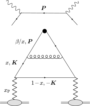
Figure 11: TMD factorisation for the (2+1)–jet contributions to diffractive SIDIS. Left panel: The soft quark case. Right panel: The soft gluon case.

Whereas the emergence of the DGLAP splitting function $P_{qq}\left({\beta}/{x}\right)$ may look natural (in view of the kinematics), what is truly remarkable is the way how this gets reconstructed from the Feynman graphs of the colour dipole picture. As visible in Eq. (138) (see also Appendix D for more details), this receives contributions from all the three graphs in Fig. 10: the direct gluon emissions by the antiquark and by the quark, and the interference piece. This is remarkable because the relative time-ordering of the two branching vertices — the photon vertex and the gluon emission vertex — appears to change when going from the projectile picture (as illustrated by the amplitude graphs in Sects. 3 and also by the cross-section graphs in Fig. 10) to the target picture, cf. the left panel of Fig. 11. One should however keep in mind that the time variables are different in the two pictures: the role of “time” is played by $x^{+}$ in the colour dipole and by $x^{-}$ in the target picture.

The splitting function $P_{qq}(\beta/x)$ exhibits a pole at $x=\beta$, which in the target picture has an obvious physical interpretation: it corresponds to the emission of a soft gluon in the $s$–channel, see the left panel in Fig. 11. It is interesting to clarify the origin of this pole in the colour dipole picture. The analysis in Appendix D shows that the singular piece of $P_{qq}(\beta/x)$ is exclusively generated by the first process in Fig. 10 — a gluon emission by the antiquark in the final state. It is well known that such final-state emissions develop collinear singularities from integrating over large formation times. In this case, the relevant formation time reads $\tau_{f}\simeq 2\vartheta_{2}\vartheta_{3}q^{+}/P_{\perp}^{2}$ and becomes arbitrarily large in the collinear limit $P_{\perp}\to 0$. Using Eq. (133) for $\vartheta_{2}\vartheta_{3}$, one finds $\tau_{f}\sim\tau_{\gamma}/(x-\beta)$ (with $\tau_{\gamma}=2q^{+}/Q^{2}$ the coherence time of the virtual photon), which confirms that the singularity at $x=\beta$ corresponds to a large formation time. Hence, the soft singularity of the hard splitting in the target picture is inherited from a collinear singularity in the projectile picture.

In the standard formulation of the DGLAP evolution, the poles of the splitting functions associated with soft gluon emissions are screened by the plus prescription, as introduced by the virtual corrections. Here, however, the virtual corrections are missing since we measure the transverse momentum $P_{\perp}$ of the daughter antiquark. (The compensation of soft divergences between real and virtual emissions should only hold in more inclusive processes, in which $P_{\perp}$ is integrated as well; see the discussion at the end of this section.) Instead, the would-be logarithmic divergence of the integral over $x$ is cut off by the explicit lower limit $x_{\rm min}$ in Eq. (141), which follows from Eq. (133). This generates a logarithmically enhanced contribution $\ln[1/(x_{\rm min}-\beta)]\simeq\ln(Q^{2}/P_{\perp}^{2})$ which is divergent when $P_{\perp}\to 0$, thus reflecting the original collinear singularity in the projectile picture.

The LT contribution of 2+1 diffractive jets with a soft gluon to diffractive SIDIS can be similarly computed (see Appendix D for details) and the result looks indeed similar to Eq. (141), namely

$$\frac{{\rm d}\sigma^{\gamma_{\scriptscriptstyle T}^{*}A\rightarrow q\bar{q}(g)A}}{{\rm d}^{2}\bm{P}\,{\rm d}\ln(1/\beta)} \,=\frac{4\pi^{2}\alpha_{\rm em}}{Q^{2}}\left(\sum e_{f}^{2}\right)\,\frac{\alpha_{s}}{\pi^{2}}\,\frac{1}{P_{\perp}^{2}}\,\int_{\beta}^{1}\frac{{\rm d}x}{x}\,\frac{\beta}{x}\ P_{qg}\left(\frac{\beta}{x}\right)xG_{\mathbb{P}}\left(x,x_{\mathbb{P}},(1-x)P_{\perp}^{2}\right),$$ (142)

where

$$P_{qg}(z)=\frac{z^{2}+(1-z)^{2}}{2}$$ (143)

is the DGLAP splitting function for the process $g\to q\bar{q}$. Once again, this result corresponds to asymmetric hard dijets, that is, to $q\bar{q}$ pairs with $\vartheta_{1}\vartheta_{2}\ll 1$. For instance, if the measured jet is the quark, the “plus” longitudinal momenta of the final partons obey the strong ordering condition (compare to Eq. (137))

$$\vartheta_{1}\,\simeq\,1\,\gg\,\vartheta_{2}\,\sim\,\frac{P_{\perp}^{2}}{Q^{2}}\,\gg\,\vartheta_{3}\,\sim\,\frac{Q_{s}^{2}}{Q^{2}}\,.$$ (144)

For a measured antiquark, the variables $\vartheta_{1}$ and $\vartheta_{2}$ get exchanged with each other.

Eq. (142) has a natural interpretation as target evolution, shown in the right panel of Fig. 11: a gluon from the Pomeron wavefunction with longitudinal momentum fraction $x$ undergoes a hard splitting into a $q\bar{q}$ pair. Either the quark, or the antiquark, from this pair absorbs the virtual photon and emerges in the final state with “minus” longitudinal fraction $x_{\rm\scriptscriptstyle Bj}$ and “plus” longitudinal fraction close to unity. This splitting function $P_{qg}({\beta}/{x})$ has no singularity at $x\to\beta$, which explains why the lower limit of the above integral has been extended down to $\beta$. This was to be expected: the original process in the dipole picture, cf. Fig. 7, involves no final-state emission, hence there is no associated collinear divergence. This argument also explains why this particular process brings no additional LT contribution from symmetric $q\bar{q}$ pairs ($\vartheta_{1}\vartheta_{2}\sim 1/4$), as will be explicitly verified in Appendix D.

At this level it should be clear that the LT contributions to diffractive SIDIS shown in Eqs. (141)–(142) describe diffractive measurements of the (anti)quark distribution in the target and hence can be interpreted as contributions to the quark diffractive TMD. Formally, these are next-to-leading order corrections, as they are suppressed by a factor $\alpha_{s}$ compared to the respective contribution from exclusive dijets, cf. Eqs. (33)–(34). Yet, as already emphasised, they give the dominant contribution at large momenta $P_{\perp}\gg Q_{s}(Y_{\mathbb{P}})$, where the LO result is strongly suppressed. As shown by the previous discussion, they should be viewed as the result of one step in the DGLAP evolution of the LO distribution (34). It is in fact natural to add together these various contributions and write

$$\frac{{\rm d}\sigma^{\gamma_{\scriptscriptstyle T}^{*}A\rightarrow(q\,{\rm or}\,\bar{q})XA}}{{\rm d}^{2}\bm{P}\,{\rm d}\ln(1/\beta)} \,=\,\frac{{\rm d}\sigma^{\gamma_{\scriptscriptstyle T}^{*}A\rightarrow q\bar{q}A}}{{\rm d}^{2}\bm{P}\,{\rm d}\ln(1/\beta)}+2\,\frac{{\rm d}\sigma^{\gamma_{\scriptscriptstyle T}^{*}A\rightarrow(q)\bar{q}gA}}{{\rm d}^{2}\bm{P}\,{\rm d}\ln(1/\beta)}+\frac{{\rm d}\sigma^{\gamma_{\scriptscriptstyle T}^{*}A\rightarrow q\bar{q}(g)A}}{{\rm d}^{2}\bm{P}\,{\rm d}\ln(1/\beta)}$$

$$\,\equiv\,\frac{4\pi^{2}\alpha_{\rm em}}{Q^{2}}\left(\sum e_{f}^{2}\right)\,2\,\frac{{\rm d}xq_{\mathbb{P}}(x,x_{\mathbb{P}},P_{\perp}^{2})}{{\rm d}^{2}\bm{P}}\bigg{|}_{x=\beta}$$ (145)

with the following approximation for the quark diffractive TMD:

$$\frac{{\rm d}xq_{\mathbb{P}}(x,x_{\mathbb{P}},P_{\perp}^{2})}{{\rm d}^{2}\bm{P}}\,=\,\frac{{\rm d}xq_{\mathbb{P}}^{q\bar{q}}(x,x_{\mathbb{P}},P_{\perp}^{2})}{{\rm d}^{2}\bm{P}}\,+\,\frac{{\rm d}xq_{\mathbb{P}}^{(q)\bar{q}g}(x,x_{\mathbb{P}},P_{\perp}^{2})}{{\rm d}^{2}\bm{P}}\,+\,\frac{{\rm d}xq_{\mathbb{P}}^{q\bar{q}(g)}(x,x_{\mathbb{P}},P_{\perp}^{2})}{{\rm d}^{2}\bm{P}}.$$ (146)

The first term in the r.h.s. is the exclusive $q\bar{q}$ pair contribution from Eq. (34), the second term comes from 2+1 jets with a soft quark and can be read off Eq. (141), while the third term refers to 2+1 jets with a soft gluon and can be inferred from Eq. (142). Specifically,

$$\frac{{\rm d}xq_{\mathbb{P}}^{(q)\bar{q}g}(x,x_{\mathbb{P}},P_{\perp}^{2})}{{\rm d}^{2}\bm{P}} \,=\,\frac{\alpha_{s}}{2\pi^{2}}\,\frac{1}{P_{\perp}^{2}}\,\int_{x}^{z_{\rm max}}{\rm d}z\,P_{qq}(z)\,\frac{x}{z}q_{\mathbb{P}}\left(\frac{x}{z},x_{\mathbb{P}},P_{\perp}^{2}\right),$$

$$\frac{{\rm d}xq_{\mathbb{P}}^{q\bar{q}(g)}(x,x_{\mathbb{P}},P_{\perp}^{2})}{{\rm d}^{2}\bm{P}} \,=\,\frac{\alpha_{s}}{2\pi^{2}}\,\frac{1}{P_{\perp}^{2}}\,\int_{x}^{1}{\rm d}z\,P_{qg}(z)\,\frac{x}{z}G_{\mathbb{P}}\left(\frac{x}{z},x_{\mathbb{P}},P_{\perp}^{2}\right),$$ (147)

where we have changed the notations a bit as compared to the previous formulae. The variable denoted as $x$ in Eqs. (146)–(5) — the longitudinal fraction of the measured (anti)quark w.r.t. the Pomeron — was previously denoted as $\beta$ in Eqs. (141)–(142). Also, the integration variable in Eq. (5) is the splitting fraction $z$ of the daughter (anti)quark at the hard vertex (previously denoted as $\beta/x$). The upper limit $z_{\rm max}$ on $z$ corresponds to the lower limit $x_{\rm min}$ in the original equations and has been obtained as $z_{\rm max}=\beta/x_{\rm min}=1/(1+4P_{\perp}^{2}/Q^{2})\simeq 1-4P_{\perp}^{2}/Q^{2}$. Finally, the virtuality argument of the diffractive PDF has been approximated as $P_{\perp}^{2}$.

At this level, it is intuitively clear that the analog of Eq. (146) for the case of the gluon diffractive TMD reads as follows

$$\frac{{\rm d}xG_{\mathbb{P}}(x,x_{\mathbb{P}},P_{\perp}^{2})}{{\rm d}^{2}\bm{P}}\,=\,\frac{{\rm d}xG_{\mathbb{P}}^{gg}(x,x_{\mathbb{P}},P_{\perp}^{2})}{{\rm d}^{2}\bm{P}}\,+\,2n_{f}\frac{{\rm d}xG_{\mathbb{P}}^{(q)\bar{q}g}(x,x_{\mathbb{P}},P_{\perp}^{2})}{{\rm d}^{2}\bm{P}}\,+\,\frac{{\rm d}xG_{\mathbb{P}}^{(g)gg}(x,x_{\mathbb{P}},P_{\perp}^{2})}{{\rm d}^{2}\bm{P}},$$ (148)

where the first piece is the tree-level contribution (the direct production of a semi-hard $gg$ dipole by the Pomeron), as appearing in the TMD factorisation for $q\bar{q}g$ jets with a soft gluon Iancu:2022lcw , cf. Eqs. (59)–(63), while the two other contributions involve convolutions between the quark or gluon DPDF and one hard vertex. Specifically, the contribution with upper index $(q)\bar{q}g$ refers to the case where the Pomeron first produces a semi-hard $q\bar{q}$ dipole and then the quark (or the antiquark) from this pair decays into a hard quark-gluon system; this is similar to Eq. (141) except that, now, it is the hard gluon that is measured by the TMD:

$$\frac{{\rm d}xG_{\mathbb{P}}^{(q)\bar{q}g}(x,x_{\mathbb{P}},P_{\perp}^{2})}{{\rm d}^{2}\bm{P}}\,=\,\frac{\alpha_{s}}{2\pi^{2}}\,\frac{1}{P_{\perp}^{2}}\,\int_{x}^{1}{\rm d}z\,P_{gq}(z)\,\frac{x}{z}q_{\mathbb{P}}\left(\frac{x}{z},x_{\mathbb{P}},P_{\perp}^{2}\right).$$ (149)

Finally, the contribution with upper index ${(g)gg}$ refers to the case where the Pomeron first produces a semi-hard gluon-gluon pair and then one of these gluons splits into a hard $gg$ pair:

$$\frac{{\rm d}xG_{\mathbb{P}}^{(g)gg}(x,x_{\mathbb{P}},P_{\perp}^{2})}{{\rm d}^{2}\bm{P}}\,=\,\frac{\alpha_{s}}{\pi^{2}}\,\frac{1}{P_{\perp}^{2}}\,\int_{x}^{z_{\rm max}}{\rm d}z\,P_{gg}(z)\,\frac{x}{z}G_{\mathbb{P}}\left(\frac{x}{z},x_{\mathbb{P}},P_{\perp}^{2}\right),$$ (150)

where the splitting function reads

$$P_{gg}(z)=2N_{c}\left[\frac{1-z}{z}+z(1-z)+\frac{z}{(1-z)}\right].$$ (151)

These two contributions to the gluon DTMD could be probed via (3+1)–jet processes involving two steps of DGLAP evolution: the hard gluon produced either in (149), or in (150), splits into an even harder $q\bar{q}$ pair and one of the daughter fermions is absorbing the virtual photon.

The previous equations in this section have the right structure to signal the emergence of the DGLAP evolution for the diffractive, quark and gluon, PDFs. Roughly speaking, the quantities in the l.h.s.’s of Eqs. (146) and (148) can be seen as the momentum derivatives of the respective DPDFs, whereas the r.h.s.’s of these equations describe the change in the diffractive distributions due to one hard splitting. There are however some noticeable differences w.r.t. the standard structure of the DGLAP equations in the literature: (i) the absence of the virtual contributions and, related to that, the appearance of the upper cutoff $z_{\rm max}<1$ in the integration over the splitting fraction $z$, and (ii) the presence of an additional, tree-level, piece, representing the respective (quark or gluon) diffractive TMD as computed in the colour dipole picture, which acts as a source for the corresponding PDFs.

The virtual DGLAP contributions were naturally absent in our previous results, which focused on the explicit production of hard partons via the (hard) splitting of semi-hard ones. But clearly, they must be added when such hard splittings get iterated; this in particular amounts to endowing the DGLAP splitting functions with the plus prescription. The source term represents the essential new ingredient provided by our analysis: it enables one to explicitly construct the quark and gluon diffractive PDFs at small $x_{\mathbb{P}}$ via calculations in the dipole picture. The complete DGLAP equations emerging from our formalism will be presented and solved in the next section. Using their solutions, we shall in particular compute the diffractive structure function $F_{2}^{D}$ according to (cf. Eq. (4))

$$x_{\mathbb{P}}F_{2}^{D(3)}(x_{\rm\scriptscriptstyle Bj},x_{\mathbb{P}},Q^{2})=2\sum_{f}e_{f}^{2}\,xq_{\mathbb{P}}(x,x_{\mathbb{P}},Q^{2})\big{|}_{x=\beta}.$$ (152)

We conclude this section with a few remarks on the remaining LT contribution to the cross-section for diffractive SIDIS, which as announced is associated with (2+1)–jet processes whose final states comprises a soft quark ($\vartheta_{1}\sim Q_{s}^{2}/Q^{2}\ll 1$) and a relatively symmetric antiquark-gluon dijet ($\vartheta_{2}\vartheta_{3}\sim 1/4$). As explained in Appendix D, this contribution comes exclusively from the the first process in Fig. 10, where the gluon is emitted by the antiquark in the final state. Besides the LT contribution showing a logarithmic singularity at $x=\beta$, that was included in Eq. (141), this process also generates a contribution which exhibits stronger, power-like, singularities and which is therefore controlled by the lower limit $x_{\rm min}$ of the integral over $x$, that is, by values of $x$ close to $\beta$. Recall that $x$ is the longitudinal momentum fraction of a semi-hard antiquark in the wavefunction of the Pomeron. Hence, the fact that $x\simeq\beta$ implies that the virtual photon is absorbed by this semi-hard antiquark, prior to its hard splitting. Accordingly, this particular LT contribution, as explicitly computed in Eq. (D.1), it is likely to correspond to final-state radiation also in the target picture. Still in Appendix D, we show in Fig. 24 a numerical comparison between the LT contributions generated by symmetric and asymmetric $\bar{q}g$ dijets, Eqs. (D.1) and respectively (141). We see that the latter dominates, especially at small $4\beta P_{\perp}^{2}/Q^{2}$, where the integral in Eq. (141) grows logarithmically.

6 The parton distributions of the Pomeron

While in the previous sections (and notably in Sect. 2.5) we have presented qualitative estimates for the quark DTMD and the quark DPDF, our goal here will be their more accurate determination, via both analytic and numerical studies. Many of the characteristic features that we shall find are similar to those of the diffractive gluon distributions, as thoroughly studied in Iancu:2022lcw . Inevitably we will repeat some parts of that previous analysis in order to work out the quark case. In the process, and for the sake of comparison, we will review some features of the gluon case. The basic ingredient in calculating the (quark and gluon) diffractive distributions is the scattering amplitude $\mathcal{T}(R,Y_{\mathbb{P}})$ in the appropriate representation of the colour group. In what follows we shall give analytic expressions relying on the MV model McLerran:1993ni ; McLerran:1994vd valid at moderate values of $\alpha_{s}Y_{\mathbb{P}}\ll 1$. For higher values such that $\alpha_{s}Y_{\mathbb{P}}\gtrsim 1$, we will resort to numerical solutions to the BK equation Balitsky:1995ub ; Kovchegov:1999yj and its collinear improvement Iancu:2015vea ; Ducloue:2019ezk . Finally we will study the (coupled) DGLAP evolution of the quark and gluon DPDFs.

6.1 The quark DTMD at tree-level

The quark DTMD at tree level is defined in Eq. (34), where the dimensionless scalar quantity $\mathcal{Q}_{\mathbb{P}}(x,x_{\mathbb{P}},K_{\perp}^{2})$ is given in Eq. (35), where we recall that $\mathcal{M}^{2}=\frac{x}{1-x}K_{\perp}^{2}$.

We first present analytic estimates based on the MV model, cf. Eq. (43). We start with the saturation regime at relatively low transverse momenta $K_{\perp}\lesssim\tilde{Q}_{s}(x)$, with $\tilde{Q}_{s}^{2}(x)=(1-x)Q_{s}^{2}$ (recall Eq. (52)). Then the integral in Eq. (35) is dominated by large dipoles of size $R\gtrsim 1/Q_{s}$, for which the MV model is well approximated by a Gaussian (a.k.a. “the GBW model” GolecBiernat:1999qd ): $\mathcal{T}(R)\simeq 1-e^{-R^{2}Q_{s}^{2}/4}$, with $Q_{s}$ the saturation momentum defined in Eq. (44). We will obtain fully analytical results for the two limiting cases $x\to 0$ and $x\to 1$ and then extrapolate some of their features to generic values of $x$. When $x\ll 1$, or equivalently when $\mathcal{M}\ll K_{\perp}$, Eq. (35) simplifies to

$$\mathcal{Q}_{\mathbb{P}}(x,K_{\perp}^{2})\simeq\mathcal{M}\int_{0}^{\infty}\!{\rm d}R\,J_{1}(K_{\perp}R)\left(1-e^{-R^{2}Q_{s}^{2}/4}\right)\simeq\sqrt{x}\,e^{-K_{\perp}^{2}/Q_{s}^{2}}\quad{\rm for}\quad K_{\perp}\lesssim Q_{s},\,\,x\ll 1,$$ (153)

which exhibits Gaussian momentum broadening. When $1-x\ll 1$, hence $\mathcal{M}\gg K_{\perp}$, Eq. (35) becomes

$$\mathcal{Q}_{\mathbb{P}}(x,K_{\perp}^{2}) \simeq\frac{\mathcal{M}^{2}K_{\perp}}{2}\int_{0}^{\infty}{\rm d}R\,R^{2}K_{1}(\mathcal{M}R)\left(1\!-\!e^{-R^{2}Q_{s}^{2}/4}\right)$$

$$\simeq\sqrt{1-x}\left[1-\frac{K_{\perp}^{2}}{\tilde{Q}_{s}^{2}}+\frac{K_{\perp}^{4}}{\tilde{Q}_{s}^{4}}\,e^{K_{\perp}^{2}/\tilde{Q}_{s}^{2}}E_{1}\big{(}K_{\perp}^{2}/\tilde{Q}_{s}^{2}\big{)}\right]\quad{\rm for}\quad K_{\perp}\lesssim\tilde{Q}_{s},\,\,1-x\ll 1,$$ (154)

where $E_{1}(z)=\int_{z}^{\infty}{\rm d}t\,e^{-t}/t$ is the exponential integral function. While the above formulae reduce to the black disk limit expression (51) when $K_{\perp}\ll\tilde{Q}_{s}$ as they should, it is important to notice that they are valid in a wide region which extends up to momenta of the order of $\tilde{Q}_{s}$. (In particular, when expanding for $K_{\perp}\ll\tilde{Q}_{s}$, Eqs. (153) and (6.1) have the same dependence on $K_{\perp}$ up to quadratic order and they start to differ only at the fourth order.) These analytic approximations predict “geometric scaling” — the function $\mathcal{Q}_{\mathbb{P}}(x,K_{\perp}^{2})/\sqrt{x(1-x)}$ appears to depend upon $K_{\perp}$ and $x$ only via the ratio $K_{\perp}/\tilde{Q}_{s}(x)$ — and we expect this property to be quite robust: a similar property should be well satisfied by the exact result in the saturation regime. Recalling the definition (34) of the quark occupation number in the Pomeron, we therefore expect the following scaling behaviour:

$$\frac{\Psi_{\mathbb{P}}(x,K_{\perp}^{2})}{x}\simeq F(K_{\perp}/\tilde{Q}_{s}(x))\quad\textrm{for}\quad K_{\perp}\lesssim\tilde{Q}_{s}(x).$$ (155)

Making use of Eqs. (153) and (6.1), we can also estimate the scaling violation in the transition regime around $\tilde{Q}_{s}$; for example at $K_{\perp}=\tilde{Q}_{s}/2$ we have

$$\frac{\big{[}\Psi_{\mathbb{P}}(x,K_{\perp}=\tilde{Q}_{s}/2)/x\big{]}_{x\to 1}}{\big{[}\Psi_{\mathbb{P}}(x,K_{\perp}=\tilde{Q}_{s}/2)/x\big{]}_{x\to 0}}=\left[\frac{12e^{1/4}+\sqrt{e}E_{1}(1/4)}{16}\right]^{2}\simeq 1.15,$$ (156)

meaning a small violation of 15%. However, this violation rapidly increases when increasing $K_{\perp}$ above $\tilde{Q}_{s}/2$, to reach about 160% at $K_{\perp}=\tilde{Q}_{s}$ (see also the left panel in Fig. 12).

Let us also consider large transverse momenta $K_{\perp}\gg\tilde{Q}_{s}$. Then the integration in Eq. (35) is controlled by small dipoles of size $R\ll 1/Q_{s}$ and one can replace the MV model amplitude with its single scattering approximation, that is $\mathcal{T}(R)\simeq(R^{2}Q_{A}^{2}/4)\ln(4/R^{2}\Lambda^{2})$. This calculation has been performed for arbitrary $x$ in Appendix B, but to our purposes here it suffices to present only the leading terms in the usual limiting cases. Using Eqs. (203) and (202) we readily obtain

$$\frac{\Psi_{\mathbb{P}}(x,K_{\perp}^{2})}{x}\simeq\frac{1}{2\pi}\begin{cases}{\displaystyle\frac{Q_{A}^{4}}{K_{\perp}^{4}}}&\quad\mathrm{for}\quad K_{\perp}\gg Q_{s},\,\,x\ll 1\\[14.22636pt] {\displaystyle\frac{4(1-x)^{2}Q_{A}^{4}}{K_{\perp}^{4}}\,\ln^{2}\frac{K_{\perp}^{2}}{(1-x)\Lambda^{2}}}&\quad\mathrm{for}\quad K_{\perp}\gg\tilde{Q}_{s},\,\,1-x\ll 1.\end{cases}$$ (157)

We note that when we express $Q_{A}^{2}$ in terms of the saturation momentum $Q_{s}^{2}$, cf. Eq. (44), the factor $(1-x)^{2}$ in the second case of the above can be absorbed into the dependence on the effective saturation scale $\tilde{Q}_{s}(x)$. Eventually this indicates that, even though Eq. (157) does not scale with $K_{\perp}/\tilde{Q}_{s}(x)$, the scaling violation happens only through a logarithmic (and not a power) dependence on $x$.

The MV model, on which the above analysis in based, is valid when the diffractive gap $Y_{\mathbb{P}}$ is not too large, such that $\alpha_{s}Y_{\mathbb{P}}\ll 1$. High energy evolution becomes relevant when $Y_{\mathbb{P}}\gtrsim 1/\alpha_{s}$ and is taken into account by solving the BK equation Balitsky:1995ub ; Kovchegov:1999yj , or more precisely its collinearly improved version Beuf:2014uia ; Iancu:2015vea ; Ducloue:2019ezk . Using the MV model amplitude $\mathcal{T}(R)$ as an initial condition at $Y_{0}$ (typically $Y_{0}\sim 4$), one solves numerically this equation to obtain the amplitude $\mathcal{T}(R,Y_{\mathbb{P}})$ at $Y_{\mathbb{P}}=Y_{0}+\Delta Y_{\mathbb{P}}$. The solution $\mathcal{T}(R,Y_{\mathbb{P}})$ is characterised by a saturation momentum $Q_{s}(Y_{\mathbb{P}})$ which increases with $Y_{\mathbb{P}}$. For large dipole sizes $R\gg 1/Q_{s}(Y_{\mathbb{P}})$, the solution approaches the black disk limit $\mathcal{T}(R,Y_{\mathbb{P}})=1$. For small dipoles with $R\ll 1/Q_{s}(Y_{\mathbb{P}})$, it exhibits the slightly softer tail (in comparison to the MV model) $\mathcal{T}(R,Y_{\mathbb{P}})\sim[R^{2}Q_{s}^{2}(Y_{\mathbb{P}})]^{\gamma}$ with $1/2<\gamma<1$ ($\gamma\simeq 0.63$ for the leading logarithmic evolution and for asymptotically high $Y_{\mathbb{P}}$). Therefore, the high energy evolution will not alter the main qualitative features of the quark DTMD, except from modifying its hard momentum behaviour to $[\tilde{Q}_{s}^{2}(x,Y_{\mathbb{P}})/K_{\perp}^{2}]^{2\gamma}$.

For the numerical implementation we regularize the infrared limit of the MV model according to

$$\mathcal{T}(R)=1-\exp\left[-\frac{Q_{A}^{2}R^{2}}{2}\ln\left(\frac{2}{\Lambda R}+e\right)\right].$$ (158)

Such a scattering amplitude is evolved in $Y_{\mathbb{P}}$ according to the collinearly improved BK evolution Ducloue:2019ezk with the precise conventions given in Appendix D in Iancu:2020jch . The corresponding amplitude in the adjoint representation at large-$N_{c}$ is determined by

$$\mathcal{T}_{g}(R,Y_{\mathbb{P}})=1-[1-\mathcal{T}(R,Y_{\mathbb{P}})]^{2}.$$ (159)

For the purposes of the numerical calculations we shall use a slightly modified definition of the saturation scale (than the one we have used so far for the analytical calculations and estimates, cf. Eq. (44) in the MV model), namely $\mathcal{T}(R=2/Q_{s},Y_{\mathbb{P}})=1/2$ and similarly for $Q_{s,g}$. We choose the value of $Q_{A}^{2}$ in Eq. (158) in such a way that the initial adjoint saturation momentum at $Y_{0}$ is $Q_{s,g}^{2}=2\,\mathrm{GeV}^{2}$, while we also fix the QCD scale to $\Lambda=0.2\,\mathrm{GeV}$. In turn, this leads to $Q_{s}^{2}=0.88\,\mathrm{GeV}^{2}$ for the saturation momentum in the fundamental representation.

In Fig. 12 we present the results of the numerical calculation of the quark DTMD, which confirm all the properties presented in this section. In this plot, we have scaled the distribution with a factor $K_{\perp}/\tilde{Q}_{s}(x)$, in order to exhibit the radial distribution in $K_{\perp}$ and thus emphasise the fact that its bulk is concentrated at low momenta $K_{\perp}\lesssim\tilde{Q}_{s}$. The numerical results show that the scaling in Eq. (155) is rather good in the regime $K_{\perp}\lesssim\tilde{Q}_{s}/2$ and violated when $K_{\perp}\gg\tilde{Q}_{s}$, while we also observe the aforementioned softening of the high momentum behavior induced by the BK evolution. For comparison, in Fig. 13 we also show the respective results for the gluon DTMD Iancu:2022lcw . As anticipated, the qualitative behaviour (notably, the approximate geometric scaling and the pattern of its violation, the existence of a pronounced peak around $K_{\perp}=\tilde{Q}_{s}$ and the power law decay at larger momenta) is very similar for quarks and gluons.

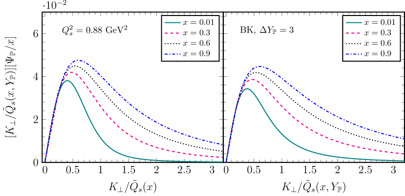
Figure 12: The quark DTMD as obtained numerically from Eqs. (34) and (35), scaled with $[K_{\perp}/\tilde{Q}_{s}(x,Y_{\mathbb{P}})]/x$ and plotted as a function of $K_{\perp}/\tilde{Q}_{s}(x,Y_{\mathbb{P}})$, for various values of $x$ and $Y_{\mathbb{P}}$. Left panel: $\mathcal{T}({R})$ is given by the MV model with a saturation scale $Q_{s}^{2}=0.88\,\mathrm{GeV}^{2}$ (in the fundamental representation). Right panel: $\mathcal{T}({R,Y_{\mathbb{P}}})$ is obtained from the solution to the collinearly improved BK equation with the initial condition at $Y_{0}$ given by the MV model. The respective saturation scale is $Q_{s}^{2}(\Delta Y_{\mathbb{P}}=3)=1.5\,\mathrm{GeV}^{2}$.

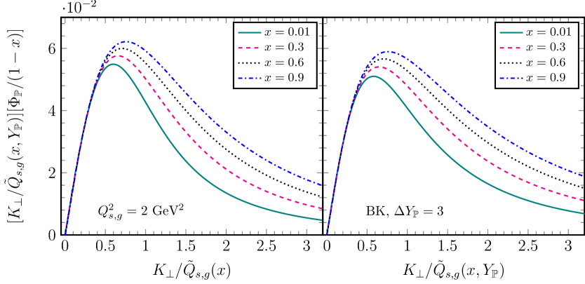
Figure 13: The gluon DTMD as obtained numerically from Eqs. (62) and (63), scaled with $[K_{\perp}/\tilde{Q}_{s,g}(x,Y_{\mathbb{P}})]/(1-x)$ and plotted as a function of $K_{\perp}/\tilde{Q}_{s,g}(x,Y_{\mathbb{P}})$, for various values of $x$ and $Y_{\mathbb{P}}$. The amplitude in the adjoint representation is determined by Eq. (159), where the amplitude $\mathcal{T}(R,Y_{\mathbb{P}})$ in the fundamental is obtained as in Fig. 12. Left panel: MV model calculation with a corresponding adjoint saturation scale $Q_{s,g}^{2}=2\,\mathrm{GeV}^{2}$. Right panel: collinearly improved BK calculation with a corresponding adjoint saturation scale $Q_{s,g}^{2}(\Delta Y_{\mathbb{P}}=3)=3.9\,\mathrm{GeV}^{2}$.

6.2 The quark DPDF at tree level

Now we turn our attention to the quark DPDF $xq_{\mathbb{P}}(x,x_{\mathbb{P}},P_{\perp}^{2})$ defined in Eq. (54) for large momenta such that $P_{\perp}^{2}\gg\tilde{Q}^{2}_{s}(x,Y_{\mathbb{P}})$. As we have already seen, the unintegrated distribution, whether obtained in the MV model or from the solution to the BK equation, falls fast enough for momenta larger than the saturation momentum so that it is integrable. Hence, the dependence of the quark DPDF on $P_{\perp}^{2}$ is rather weak and to a first approximation we can take $P_{\perp}^{2}\to\infty$. Eventually the integrand is controlled by momenta of the order of $\tilde{Q}_{s}(x,Y_{\mathbb{P}})$, cf. Eq. (157) and Fig. 12, and thus the quark DPDF inherits the approximate scaling properties of the quark DTMD. We readily obtain

$$xq_{\mathbb{P}}(x,x_{\mathbb{P}},P_{\perp}^{2}=\infty)\simeq\frac{S_{\perp}N_{c}}{4\pi^{3}}\,\kappa_{q}(x)x(1-x)Q_{s}^{2}(Y_{\mathbb{P}}),$$ (160)

where $\kappa_{q}(x)$ is a slowly varying function of $x$ in the interval $[0,1]$. Its precise form depends on the details of the scattering amplitude $\mathcal{T}(R,Y_{\mathbb{P}})$, hence it also depends weakly on $Y_{\mathbb{P}}$, and can be easily determined numerically or even analytically in certain simple cases. For example, in the GBW model one can make use of Eqs. (153) and (6.1) to find Buchmuller:1998jv ; Hatta:2022lzj $\kappa_{q}(0)=1/4$ and $\kappa_{q}(1)=3\pi^{2}/16-1\simeq 0.85$. In the left panel of Fig. 14 we show $\kappa_{q}(x)$ in the GBW and MV models.

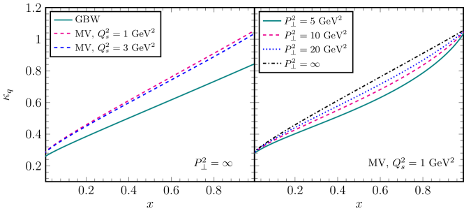
Figure 14: Left panel: The slowly varying function $\kappa_{q}(x)$ appearing in the quark DPDF in Eq. (160) for the GBW model (for which it is independent of $Q_{s}$) and for the MV model for two different saturation scales. Right panel: The function $\kappa_{q}(x,P_{\perp}^{2})$ for various values of $P_{\perp}^{2}$ (with $P_{\perp}^{2}>Q_{s}^{2}$) as a function of $x$ in the MV model with $Q_{s}^{2}=1$ GeV².

One can generalize Eq. (160) to include the mild dependence on $P_{\perp}^{2}$ by writing

$$xq_{\mathbb{P}}(x,x_{\mathbb{P}},P_{\perp}^{2})\simeq\frac{S_{\perp}N_{c}}{4\pi^{3}}\,\kappa_{q}(x,x_{\mathbb{P}},P_{\perp}^{2})x(1-x)Q_{s}^{2}(Y_{\mathbb{P}}),$$ (161)

and where it is a straightforward exercise to find that (by subtracting from Eq. (160) the contribution for momenta larger than $P_{\perp}$)

$$\kappa_{q}(x,x_{\mathbb{P}},P_{\perp}^{2})=\kappa_{q}(x)-\frac{\pi\int_{P_{\perp}^{2}}^{\infty}{\rm d}K_{\perp}^{2}\,\Psi_{\mathbb{P}}(x,x_{\mathbb{P}},K_{\perp}^{2})}{x(1-x)Q_{s}^{2}(Y_{\mathbb{P}})}.$$ (162)

Using the above and the large $K_{\perp}$ behavior of the MV model in Eq. (157), one immediately finds that the correction due to the dependence on $P_{\perp}^{2}$ is of the order of $\tilde{Q}_{s}^{2}(x)/P_{\perp}^{2}$, and therefore very small as anticipated. In the right panel of Fig. 14 we exhibit how $\kappa_{q}(x,x_{\mathbb{P}},P_{\perp}^{2})$ approaches the asymptotic line $\kappa_{q}(x)$ in the MV model.

Finally, it is clear that BK evolution will lead to an overall strong increase of the quark DPDF, since the latter is proportional to $Q_{s}^{2}(Y_{\mathbb{P}})$. This is the main dependence of the quark DPDF on $Y_{\mathbb{P}}$; indeed, as we have already pointed out $\kappa_{q}(x)$ depends very weakly on $Y_{\mathbb{P}}$ (so we have opted not to write it explicitly) while the $P_{\perp}^{2}$-dependent correction in Eq. (162) now becomes of the order of $[\tilde{Q}_{s}^{2}(x,Y_{\mathbb{P}})/P_{\perp}^{2}]^{2\gamma-1}$ and still remains very small.

In Fig. 15 we show how the quark and gluon DPDFs depend on $x$. We evaluate them at the scale $\mu_{0}^{2}=4\,\mathrm{GeV}^{2}$ for reasons which will become clear in Sect. 6.3 and with a scattering amplitude given, as usual, by the MV model or by the solution to the collinearly improved BK equation. Both panels verify the qualitative behaviour visible in Eqs. (161) (for quarks) and (68) (for gluons). For $x=0$ the quark DPDF vanishes while the gluon one is non-zero, while as $x\to 1$ the gluon vanishes faster than the quark. Moreover, confronting the right with the left panel, we also confirm the previously discussed dependence on $Y_{\mathbb{P}}$: the quark DPDF plot on the right panel is almost a perfect rescaling of the corresponding plot on the left with a factor $Q_{s}^{2}(Y_{\mathbb{P}})/Q_{s}^{2}(Y_{0})$, and similarly for the gluon.

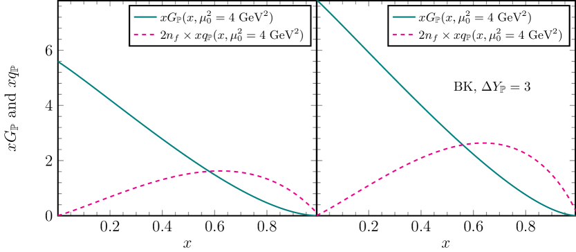
Figure 15: The quark DPDF (multiplied by the total number of active flavors including antiquarks) and the gluon DPDF as functions of $x$ evaluated at the scale $\mu_{0}^{2}=4\,\mathrm{GeV}^{2}$ and with the scattering amplitude given by the MV model (left), or by the solution to the collinearly improved BK equation (right). A factor $S_{\perp}/4\pi^{3}$ has been omitted.

6.3 DGLAP evolution of the DPDFs

When $P_{\perp}^{2}\gg Q_{s}^{2}(Y_{\mathbb{P}})$, there is a large phase space available for partonic emissions between the semi-hard jet and the hard dijet system (that is, outside the rapidity gap which remains unaltered). The dominant corrections come from emissions which are strongly ordered in transverse momenta and which express the DGLAP evolution of the parton DPDFs. As shown by our analysis of NLO corrections to diffractive SIDIS in Sect. 5, this evolution also emerges from the colour dipole picture, although our respective argument was incomplete (we did not compute the relevant virtual corrections). Assuming this to be the case, in this section we shall study the coupled DGLAP evolution of the quark and gluon DPDFs. Yet another lesson from the discussion in Sect. 5 is the fact that the tree-level results for the DTMDs naturally act as source terms in the DGLAP equations for the respective DPDFs (see also Iancu:2022lcw ; Iancu:2023lel ). Taking this into account, the relevant equations are

$$\frac{{\rm d}}{{\rm d}\ln P_{\perp}^{2}}\begin{bmatrix}xG_{\mathbb{P}}(x,x_{\mathbb{P}},P_{\perp}^{2})\\[2.84544pt] xq_{\mathbb{P}}(x,x_{\mathbb{P}},P_{\perp}^{2})\end{bmatrix}=\,\, \pi P_{\perp}^{2}\begin{bmatrix}N_{g}\Phi_{\mathbb{P}}(x,x_{\mathbb{P}},P_{\perp}^{2})\\[2.84544pt] N_{c}\Psi_{\mathbb{P}}(x,x_{\mathbb{P}},P_{\perp}^{2})\end{bmatrix}$$

$$+\frac{\alpha_{s}(P_{\perp}^{2})}{2\pi}\int_{x}^{1}{\rm d}z\begin{bmatrix}P_{gg}(z)&2n_{f}P_{gq}(z)\\[2.84544pt] P_{qq}(z)&P_{qg}(z)\end{bmatrix}\begin{bmatrix}{\displaystyle(x/z)G_{\mathbb{P}}(x/z,x_{\mathbb{P}},P_{\perp}^{2})}\\[2.84544pt] {\displaystyle(x/z)q_{\mathbb{P}}(x/z,x_{\mathbb{P}},P_{\perp}^{2})}\end{bmatrix},$$ (163)

where we have omitted a factor $S_{\perp}/4\pi^{3}$, which is common to both gluon and quark distributions and can be easily reinserted in the final results. Still, we have kept the corresponding color factors which are different, namely $N_{g}=N_{c}^{2}-1$ and $N_{c}$. The factor $2n_{f}=6$ in front of the $P_{gq}$ splitting function sums the quark and antiquark contributions from all light flavors. This simplification occurs, because in our framework all distributions for such different flavours are identical. The splitting functions in Eq. (6.3) read as follows:

$$P_{gg}(z)=2N_{c}\left[\frac{1-z}{z}+z(1-z)+\frac{z}{(1-z)_{+}}\right]+\frac{11N_{c}-2n_{f}}{6}\,\delta(1-z),$$

$$P_{gq}(z)=C_{F}\,\frac{1+(1-z)^{2}}{z},\quad P_{qq}(z)=C_{F}\,\frac{1+z^{2}}{(1-z)_{+}}+2\delta(1-z),\quad P_{qg}(z)=\frac{1}{2}\left[z^{2}+(1-z)^{2}\right].$$ (164)

As compared to their previous expressions in Sect. 5, they now include additional pieces, notably the plus prescription defined as

$$\int_{x}^{1}{\rm d}z\,\frac{f(z)}{(1-z)_{+}}\equiv\int_{x}^{1}{\rm d}z\,\frac{f(z)-f(1)}{1-z}+f(1)\ln(1-x),$$ (165)

that should be generated after adding the relevant virtual corrections. The QCD running coupling is evaluated at the one loop level, that is

$$\alpha_{s}(P_{\perp}^{2})=\frac{1}{b\ln P_{\perp}^{2}/\Lambda^{2}}\quad\mathrm{with}\quad b=\frac{11N_{c}-2n_{f}}{12\pi}.$$ (166)

In these equations, the rapidity gap $Y_{\mathbb{P}}$ plays the role of a parameter: the dependence upon $Y_{\mathbb{P}}$ only enters via the source terms, which are obtained from solutions to the BK/JIMWLK equation (as explained in the previous sections).

The solutions to Eq. (6.3) are physically meaningful only for values of the resolution scale $P_{\perp}^{2}$ which are significantly larger than the target saturation momentum $Q_{s}^{2}(Y_{\mathbb{P}})$: indeed, as already mentioned, the physical phase-space for DGLAP-like emissions is $\ln(P_{\perp}^{2}/Q_{s}^{2})$. This means that the DGLAP evolution must be “turned on” at some scale $\mu_{0}^{2}$, which is the lowest value of $P_{\perp}^{2}$ for which the effects of this evolution start to be important. Specifically, this scale should be larger than the gluon saturation momentum $Q_{s,g}^{2}$ (which is the largest between the two saturation scales), but at the same time obey $\alpha_{s}\ln(\mu_{0}^{2}/Q_{s}^{2})\ll 1$ (to avoid losing important effects of the DGLAP evolution). Different choices for $\mu_{0}^{2}$ which differ, say, by a factor of 2 should be seen as a source of scheme dependence. Accordingly, the solutions to Eq. (6.3) can be fully trusted only for sufficiently large values $P_{\perp}^{2}\gg\mu_{0}^{2}$, where this scheme dependence becomes less important. (Indeed, this dependence decreases with increasing $P_{\perp}$ above $\mu_{0}$; see e.g. Iancu:2023lel for some numerical tests.)

The most interesting values of $x$ are of the order of 1/2, i.e. they are not very close to the endpoints of the allowed kinematic regime. Still, we can get a rather useful insight to the solution of the DGLAP equations by studying analytically the two limiting cases $x\to 0$ and $x\to 1$.

(i) When $x\ll 1$, the gluon evolution is driven by the singular $2N_{c}/z$ part of the $P_{gg}(z)$ splitting function at small $z$, which leads to logarithmically enhanced contributions, as coming from the lower limit $x$ of the integral over $z$. Notice that the $P_{gq}(z)$ splitting function is singular too in that limit, but since $xq_{\mathbb{P}}(x=0,x_{\mathbb{P}},P_{\perp}^{2})=0$ at tree level (cf. Eq. (161)), the corresponding contribution will be subleading. Indeed, in order to create a non-zero quark distribution at $x=0$, a gluon must split to a $q\bar{q}$ pair and such a process does not generate a large logarithm since $P_{qg}(z)$ is finite at small $z$. It is straightforward to resum the dominant double logarithms and obtain the leading term of the gluon DPDF as Iancu:2022lcw

$$xG_{\mathbb{P}}(x,x_{\mathbb{P}},P_{\perp}^{2})\simeq N_{g}\kappa_{g}(0)Q_{s,g}^{2}(Y_{\mathbb{P}})\,I_{0}\left(\sqrt{\frac{4N_{c}}{\pi b}\ln\frac{\alpha_{s}(\mu_{0}^{2})}{\alpha_{s}(P^{2}_{\perp})}\ln\frac{1}{x}}\right)\quad\mathrm{for}\quad x\ll 1,$$ (167)

where $\mu_{0}^{2}$ is the scale at which we initiate the evolution. This gluon distribution acts also as a seed for the corresponding quark distribution. More precisely, the latter receives its dominant contribution from a series of sequential $g\to gg$ splittings followed by a single $g\to q\bar{q}$ splitting only in the very last step and we find

$$xq_{\mathbb{P}}(x,x_{\mathbb{P}},P_{\perp}^{2})\simeq\frac{N_{g}\kappa_{g}(0)Q_{s,g}^{2}(Y_{\mathbb{P}})}{3}\,\sqrt{\frac{\ln\frac{\alpha_{s}(\mu_{0}^{2})}{\alpha_{s}(P^{2}_{\perp})}}{4\pi bN_{c}\ln\frac{1}{x}}}\,I_{1}\left(\sqrt{\frac{4N_{c}}{\pi b}\ln\frac{\alpha_{s}(\mu_{0}^{2})}{\alpha_{s}(P^{2}_{\perp})}\ln\frac{1}{x}}\right)\quad\mathrm{for}\quad x\ll 1.$$ (168)

The aforementioned $g\to q\bar{q}$ transition, gives rise to the extra factor $\int_{0}^{1}{\rm d}z\,P_{qg}(z)=1/3$ in the above. To conclude, for asymptotically small values of $x$, both the gluon and the quark DPDFs increase with increasing $P_{\perp}^{2}$ and/or decreasing $x$, since they are determined by real emissions only. Needless to say, the DGLAP evolution generates a non-zero value of $xq_{\mathbb{P}}(x,x_{\mathbb{P}},P_{\perp}^{2})$ as $x\to 0$.

(ii) When $1-x\ll 1$ the second term in Eq. (165), which arises from virtual graphs and is proportional to a large $\ln(1-x)$ factor, controls the evolution as one can verify by successive iterations of the tree level term. Such a piece is present only in the diagonal splitting functions $P_{gg}(z)$ and $P_{qq}(z)$, hence it becomes clear that the two parton distributions decouple from each other. For the gluon DPDF we find Iancu:2022lcw

$$xG_{\mathbb{P}}(x,x_{\mathbb{P}},P_{\perp}^{2})\simeq N_{g}\kappa_{g}(1)Q_{s,g}^{2}(Y_{\mathbb{P}})(1-x)^{\textstyle 2+\frac{N_{c}}{\pi b}\ln\frac{\alpha_{s}(\mu_{0}^{2})}{\alpha_{s}(P^{2}_{\perp})}}\quad\mathrm{for}\quad 1-x\ll 1$$ (169)

and similarly for the quark DPDF

$$xq_{\mathbb{P}}(x,x_{\mathbb{P}},P_{\perp}^{2})\simeq N_{c}\kappa_{q}(1)Q_{s}^{2}(Y_{\mathbb{P}})(1-x)^{\textstyle 1+\frac{C_{F}}{\pi b}\ln\frac{\alpha_{s}(\mu_{0}^{2})}{\alpha_{s}(P^{2}_{\perp})}}\quad\mathrm{for}\quad 1-x\ll 1.$$ (170)

The two above expressions exhibit an increased suppression for $x\to 1$ as compared to the respective tree level results. Furthermore, both DPDFs decrease with increasing $P_{\perp}^{2}$ (in sharp contrast to what happens when $x\ll 1$), a property which is a corollary of the fact that the virtual terms drive the evolution. All this is in agreement with a physical picture in which the modes with large $x$ get depleted due to the successive branchings, whereas the emerging partons populate the modes with smaller values of $x$.

Now we move on to present numerical solutions to the DGLAP equations. In Iancu:2023lel it has been numerically confirmed that the scheme dependence related to the precise choice of $\mu_{0}^{2}$ is rather small. In what follows we shall take $\mu_{0}^{2}=4\,\mathrm{GeV}^{2}$, the value for which we presented the DPDFs at tree level in Fig. 15.

In Fig. 16 we show the $x$-dependence of the evolved DPDFs for a resolution scale $P_{\perp}^{2}=16\,\mathrm{GeV}^{2}$, for both $\Delta Y_{\mathbb{P}}=0$ (where the source terms are constructed with the MV model) and for $\Delta Y_{\mathbb{P}}=3$ (where they are obtained from the solution to the BK equation, as explained in Sect. 6.1). As $x$ approaches zero, we observe that the evolution induces a sharp increase in the gluon DPDF, which is much stronger than the one seen at tree level in Fig. 15. When $x\to 0$, the numerical solution appears to diverge, in agreement with the analytic expectation (167). Still for $x\to 0$, the quark DPDF is not vanishing any more, since its evolution is driven by the gluon distribution. The asymptotic approximation (168) predicts an increase in the quark DPDF as $x\to 0$ and the onset of this behaviour is marginally visible in Fig. 16. To better visualise this behaviour, in Fig. 17 we expand the scale at small $x$. (Clearly, the increase in the quark DPDF at small $x$ will become more and more pronounced with increasing $P_{\perp}^{2}$; see also Fig. 18.) When $1-x\ll 1$, both distributions fall faster than the corresponding tree level ones in accordance with Eqs. (169) and (170). It goes without saying that the $Y_{\mathbb{P}}$-dependence is the same as in Fig. 15, that is, in going from the left to the right panel, the DPDFs scale with the respective saturation scales, cf. Eqs. (161) and (68).

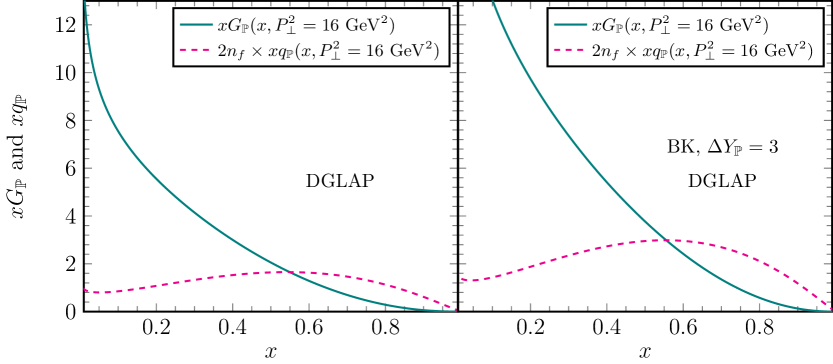
Figure 16: The DGLAP evolved quark and gluon DPDFs as functions of $x$ evaluated at the scale $P_{\perp}^{2}=16\,\mathrm{GeV}^{2}$ and with the scattering amplitude given by the MV model (left) or by the solution to the collinearly improved BK equation (right). A factor $S_{\perp}/4\pi^{3}$ has been omitted.

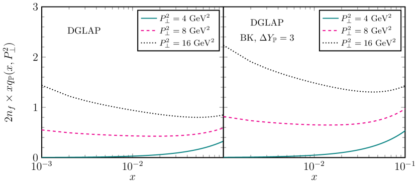
Figure 17: The quark DPDF as a function of $x$ evaluated for various values of $P_{\perp}^{2}$ and with the scattering amplitude given by the MV model (left) or by the solution to the collinearly improved BK equation (right). A factor $S_{\perp}/4\pi^{3}$ has been omitted.

In Fig. 18 we present the transverse momentum dependence of the DPDFs for various values of $x$. With increasing $P_{\perp}^{2}$ they increase when $x$ is small and they decrease when $x$ starts to get close to one (cf. the discussions below Eqs. (168) and (170)).

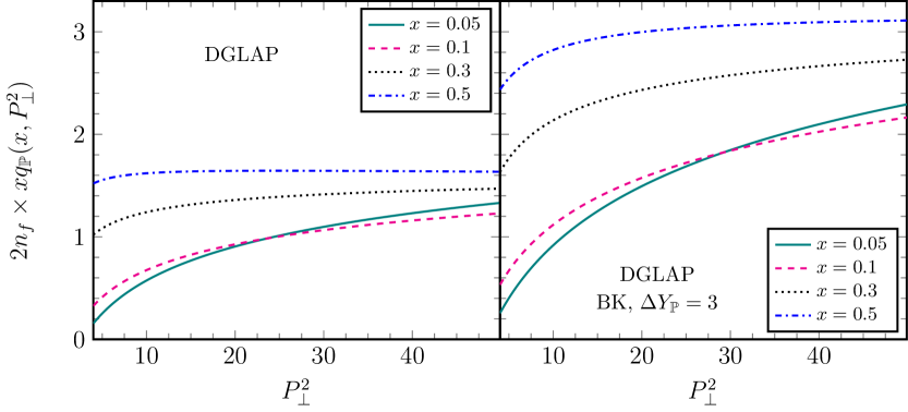
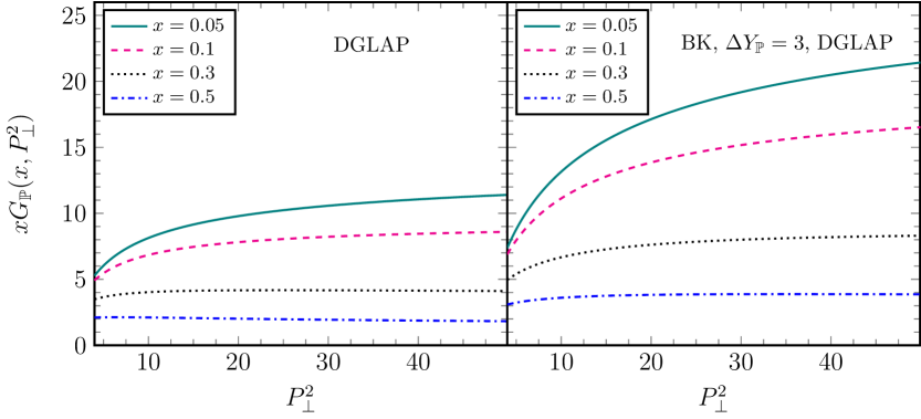
Figure 18: The DGLAP evolved quark (top panel) and gluon (bottom panel) DPDFs as functions of $P_{\perp}^{2}$ for various values of $x$. The scattering amplitude is given by the MV model (left) or by the solution to the collinearly improved BK equation (right). A factor $S_{\perp}/4\pi^{3}$ has been omitted.

To conclude this section, we would like to point out that it is possible to reformulate Eq. (6.3) as an initial value problem, which is a more standard formulation of the DGLAP evolution. To that aim, one should replace the coupled evolution equations (6.3) with sourceless equations, which are endowed with initial conditions at $P_{\perp}^{2}=\mu_{0}^{2}$, as obtained by integrating the tree-level quark and gluon DTMDs over $K_{\perp}^{2}$ either up to $\mu_{0}^{2}$, or up to infinity. (The difference between the two choices for the initial conditions should be small, and part of our scheme dependence, due to the rapid fall off of the DTMDS when $K_{\perp}^{2}\gg\tilde{Q}_{s}^{2}(x)$.) By construction, these two approaches to the DGLAP evolution — that involving the source terms and its more traditional version, which is sourceless — should lead to similar results when we evolve up to a scale $P_{\perp}^{2}$ which is much larger than $\mu_{0}^{2}$. Their differences at finite $P_{\perp}^{2}$ should be seen as a form of scheme dependence. We have numerically tested this source of scheme dependence in Fig. 19, by comparing the solutions numerically obtained in both approaches. (The initial conditions for the sourceless equations have been inferred by integrating the DTMDs over $K_{\perp}^{2}$ up to infinity.) As expected, the difference becomes negligible at large momenta, particularly for values of $x$ which are not too small. In what follows we shall use only the source term approach, since it is physically better motivated for the problem under consideration (cf. the discussion in Sect. 5).

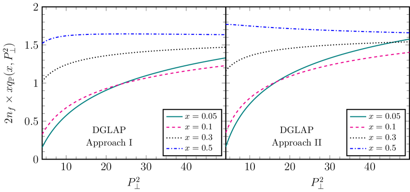
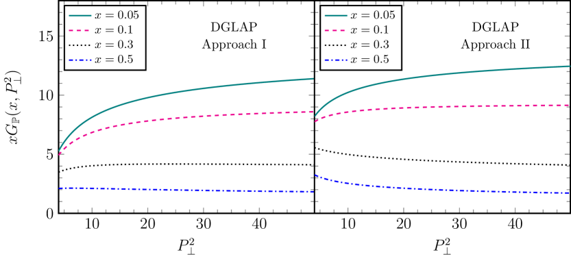
Figure 19: The DGLAP evolved quark (top panel) and gluon (bottom panel) DPDFs as functions of $P_{\perp}^{2}$ for various values of $x$, obtained by employing two different “schemes”. Left: DGLAP evolution with a source term (Approach I), as given in Eq. (6.3). DGLAP evolution as an initial value problem (Approach II), as discussed in Sect. (6.3). The scattering amplitude is given by the MV model in all panels. A factor $S_{\perp}/4\pi^{3}$ has been omitted.

6.4 The diffractive structure function

The diffractive structure function $x_{\mathbb{P}}F_{2}^{D(3)}$ has been defined in Eq. (2) and to (strict) leading order and leading twist is determined by the quark (and antiquark) DPDFs as shown in Eq. (4). At the end of Sect. 2.5 we have already looked briefly at its behaviour and also emphasised the fact that, in order to obtain a realistic behaviour near $x=1$, one must include a higher twist contribution coming from longitudinally polarised virtual photons. In Sect. 5 we have shown the emergence of the DGLAP evolution in the context of diffractive SIDIS and concluded by writing down a better approximation for $x_{\mathbb{P}}F_{2}^{D(3)}$, cf. Eq. (152), which includes the DGLAP evolution of the quark DPDF. (Strictly speaking, it is this improved approximation that should be viewed as the proper leading-order and leading twist result for the diffractive structure function.) In this section, we will revisit the tree level results presented in Sect. 2.5, by including the effects of the DGLAP evolution. It would be clearly interesting to compare our subsequent results with the predictions of the recent next-to-leading order calculation of the diffractive structure function in the colour dipole picture Beuf:2024msh .

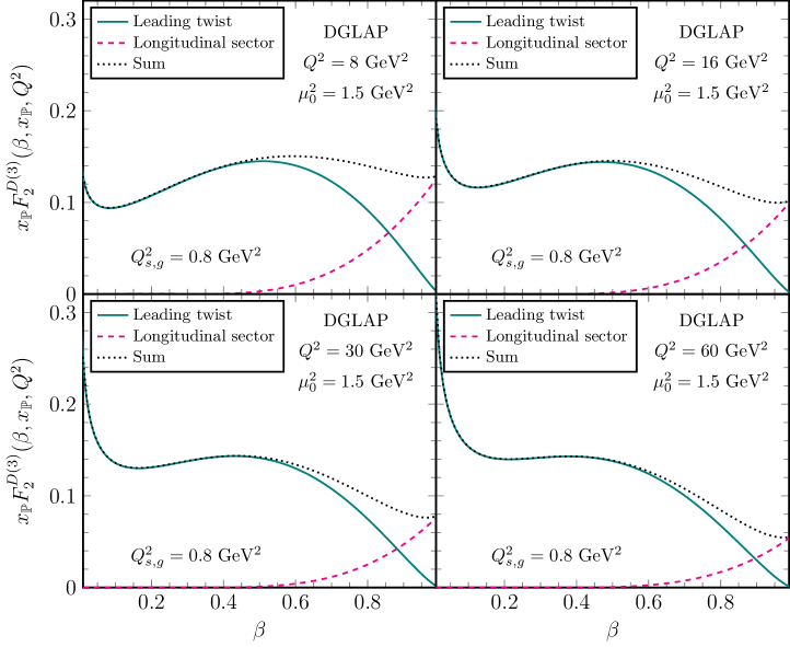
Figure 20: The proton diffractive structure function $x_{\mathbb{P}}F_{2}^{D(3)}$ and the separate contributions from the transverse (leading twist) and longitudinal sector (higher twists) as functions of $\beta$ for various values of $Q^{2}$ and for two different initial scales $\mu_{0}^{2}$. The scattering amplitude is given by the MV model with $Q_{s,g}^{2}=0.8\,\mathrm{GeV}^{2}$. A factor $S_{\perp}/4\pi^{3}$ has been omitted.

The function $x_{\mathbb{P}}F_{2}^{D(3)}$ depends upon three independent variables, that will be chosen as $\beta,\,x_{\mathbb{P}}$ and $Q^{2}$ (like in the r.h.s. of Eq. (152)). Even though we do not aim at a realistic phenomenological study, we shall nevertheless show results for two types of target: a large nucleus with tree-level (gluon) saturation momentum $Q_{s,g}^{2}=2\,\mathrm{GeV}^{2}$ and a proton described as a “small nucleus” — that is, by the MV model with a lower value for the saturation momentum, chosen as $Q_{s,g}^{2}=0.8\,\mathrm{GeV}^{2}$. The above ratio between the two saturation momenta squared is significantly smaller than the mean-field value $A^{1/6}\simeq 6$ (for $A=200$) expected at asymptotically large values of $A$. Such a smaller ratio indeed seems to be favoured by the phenomenology Ducloue:2019jmy , yet its precise value is not our main concern: clearly, the overall normalisations of the quark and gluon DPDFs are strongly sensitive to the value of $Q_{s,g}^{2}$, cf. Eqs. (161) and (68), but here we are merely interested in the functional dependences of $x_{\mathbb{P}}F_{2}^{D(3)}$, and not in its overall strength. Rather, what we would like to demonstrate is the importance of the running coupling effects in conjunction with a relatively low value for the initial scale $\mu_{0}^{2}$, as appropriate for a less dense target.

We recall that $\mu_{0}^{2}$ is the scale for the onset of the DGLAP evolution and it must be low enough to avoid losing a significant part of this evolution. For a large nucleus, we have chosen $\mu_{0}^{2}=4\,\mathrm{GeV}^{2}$, which is twice as large as the respective saturation momentum squared. Following the same argument, we will choose $\mu_{0}^{2}=1.5\,\mathrm{GeV}^{2}$ for a proton target with $Q_{s,g}^{2}=0.8\,\mathrm{GeV}^{2}$. (This value appears to be also preferred by fits to the HERA data for $x_{\mathbb{P}}F_{2}^{D(3)}$ Buchmuller:1998jv ; Golec-Biernat:2001gyl .)

In Figs. 20 and 21 we show the numerical solutions to the DGLAP equations (6.3) with the source terms given by the MV model, for a proton target and for a nuclear target, respectively (as functions of $\beta$ for several values of $Q^{2}$). We emphasise that, at tree level, these curves had exactly the same shapes for proton and nucleus, respectively (only their overall normalisations were different). So, all the differences in shape that are visible between the proton and the nuclear curves in these figures are to be attributed to the DGLAP evolution and, more precisely, to the different choices for the initial scale $\mu_{0}^{2}$ in the two cases. We have previously advocated that such differences should be seen as a form of scheme dependence. Yet, that was only the case when changing the value of $\mu_{0}^{2}$ for a fixed target. In the present case, the different choices for $\mu_{0}^{2}$ are physically motivated: the phase-space for the DGLAP evolution is bounded from below by the saturation momentum, hence it is truly different for dense and respectively dilute targets. The results in Figs. 20 and 21 reflect these physical difference and, in particular, its interplay with the running of the coupling.

When comparing the corresponding proton and nuclear curves in Figs. 20 and 21, one should distinguish the LT contributions (represented by full lines), which are sensitive to the DGLAP evolution, from the higher-twist contribution of a longitudinal photon (shown in dashed lines), which is still computed at tree-level, like in Sect. 2.5. The relative importance of the latter is larger for the nucleus than for the proton, for a trivial reason: being higher-twist, it is proportional to a larger power of $Q_{s}^{2}$ — namely to $Q_{s}^{4}$. So, in order to compare the effects of the DGLAP evolution, we shall focus on the curves represented by full lines.

The numerical results in Figs. 20 and 21 show that the effects of the evolution are considerably larger for a proton target than for a large nucleus (compare also with the tree-level results shown in Fig. 4). This is manifest both at low values of $\beta$ (where the proton diffractive structure function increases faster than the nuclear one) and at largish values of $\beta$ (where the proton curves decrease faster with increasing $\beta$). As expected, the differences become more pronounced with increasing $Q^{2}$. The difference $\ln(4/1.5)\simeq 1$ in the respective phase-spaces being small, one may wonder what is the true reason for such a different behaviour. A moment of thinking (confirmed by numerical tests) reveals that this should be mostly attributed to the running of the QCD coupling: the latter is not that small between $1.5\,\mathrm{GeV}^{2}$ and $4\,\mathrm{GeV}^{2}$, hence the contributions from this region are indeed substantial. This argument is further corroborated by the fact that a similar change in the initial scale, but from $\mu_{0}^{2}=4\,\mathrm{GeV}^{2}$ to $\mu_{0}^{2}=8\,\mathrm{GeV}^{2}$ (where the coupling is somewhat smaller), introduced only minor differences in the results Iancu:2023lel .

Although it is not in our intentions to make predictions for the phenomenology, let us nevertheless observe that the previous considerations may have interesting consequences for the DIS data. Our results for a proton target in Fig. 20, which exhibit a vivid DGLAP evolution, are qualitatively supported by the analysis of the HERA data in Ref. Golec-Biernat:2001gyl . So, assuming one can also trust our results for a nuclear target, cf. Fig. 21, we would conclude that the effects of the DGLAP evolution should be considerably less important for diffractive DIS off a large nucleus at the EIC than for diffractive DIS off a proton at HERA. For moderate values $Q^{2}\sim 10\,\mathrm{GeV}^{2}$, one might even be able to recognise the tree-level behaviour shown in Fig. 4 in the actual data.

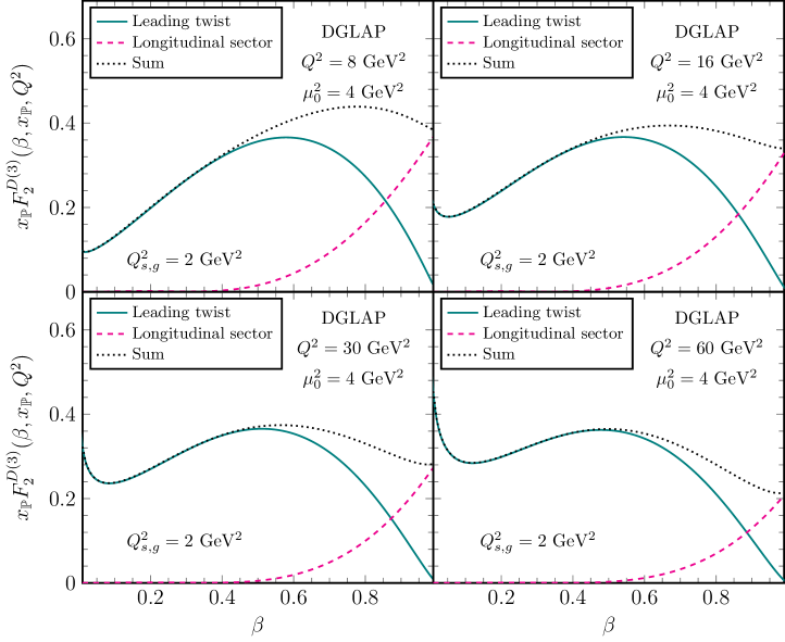
Figure 21: The nucleus diffractive structure function $x_{\mathbb{P}}F_{2}^{D(3)}$ and the separate contributions from the transverse (leading twist) and longitudinal sector (higher twists) as functions of $\beta$ for various values of $Q^{2}$, in the MV model with $Q_{s,g}^{2}=2\,\mathrm{GeV}^{2}$. A factor $S_{\perp}/4\pi^{3}$ has been omitted.

6.5 (2+1)–jet contributions to the quark DTMD

In Sect. 5 in Eq. (5) we wrote the diffractive SIDIS cross section in a factorized form in terms of the quark DTMD. The latter is a sum of three terms which are listed in Eq. (146). The first term, arises from the exclusive $q\bar{q}$ pair production and was studied in detail in Sect. 6.1. Here we shall take a closer look at the remaining two terms, i.e. to the contributions which the quark DTMD receives from the production of 2+1 jets and are explicitly given in Eq. (5).

It is important to keep in mind that the approximations underlying Eqs. (146)–(5) are valid only for hard diffractive SIDIS, that is, for the production of a quark (or antiquark) with transverse momentum $P_{\perp}$ much larger than the target saturation momentum $Q_{s}(Y_{\mathbb{P}})$ (but much smaller than the photon virtuality $Q$). Indeed, in Sect. 5 we have isolated the LT contributions in the regime $Q^{2}\gg P_{\perp}^{2}\gg Q_{s}^{2}(Y_{\mathbb{P}})$. From Sect. 2 and also Sect. 6.1, we know already that the $q\bar{q}$ contribution to diffractive SIDIS is strongly suppressed at large transverse momenta, where it decays like $Q_{s}^{4}(Y_{\mathbb{P}})/P_{\perp}^{4}$. On the other hand, the respective contributions of (2+1)–jets decay much slower, like $Q_{s}^{2}(Y_{\mathbb{P}})/P_{\perp}^{2}$, as visible in Eq. (5). This argument seems to suggest that the (2+1)–jet contributions to the r.h.s. of Eq. (146) should largely dominate over the $q\bar{q}$ contribution at any $P_{\perp}^{2}\gg Q_{s}^{2}(Y_{\mathbb{P}})$. This is roughly true for generic values of $x$, which are not too close to 1. On the other hand, when $x\to 1$, the (2+1)–jet contributions vanish faster than the tree-level ($q\bar{q}$) piece. This is due to the DGLAP evolution, which depletes the modes at large $x$, and also to kinematical constraints, like the condition $x<z_{\rm max}$ in the first integral in Eq. (5).

The above discussion helps understanding the numerical results exhibited in Fig. 22, which compare the strength of the $q\bar{q}$ piece (computed as in Sect. 6.1) with the contributions of (2+1)–jets, as functions of $x$ and for two hard values $P_{\perp}^{2}=4\,\mathrm{GeV}^{2}$ and $16\,\mathrm{GeV}^{2}$. Namely, we immediately see that 2+1 jets dominate at relatively small $x\lesssim 0.5$, whereas the exclusive dijets still prevail at larger values of $x$ (and especially near $x=1$). Interestingly, the two types of contributions are of the same order for $x$ around one half.

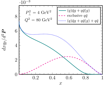
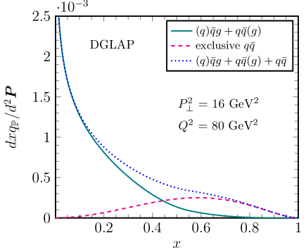
Figure 22: The total quark DTMD and its two pieces, arising from the $q\bar{q}$ dijet (cf. Eq. (34)) and, respectively, from (2+1)–jets (cf. Eq. (5)), as functions of $x$ for $P_{\perp}^{2}=4\,\mathrm{GeV}^{2}$ (left panel) and $P_{\perp}^{2}=16\,\mathrm{GeV}^{2}$ (right panel). The scattering amplitude is given by the MV model. The right panel includes the effects of the DGLAP evolution for the (2+1)–jet contributions in Eq. (5). The resolution scale $Q^{2}=80\,\mathrm{GeV}^{2}$ is necessary to fix the upper limit $z_{\rm max}=1/(1+4P_{\perp}^{2}/Q^{2})$ in the first integral (5). A factor $S_{\perp}/4\pi^{3}$ has been omitted.

Once again, it is instructive to support these numerical findings with analytical arguments. Let us start from the $q\bar{q}(g)$ piece, that is, the one where the gluon is soft, and consider first the limiting case $x\ll 1$. Making use of Eq. (167) and performing the longitudinal fraction integration we obtain the leading behavior

$$\frac{{\rm d}xq_{\mathbb{P}}^{q\bar{q}(g)}(x,x_{\mathbb{P}},P_{\perp}^{2})}{{\rm d}\ln P_{\perp}^{2}}\simeq\frac{\alpha_{s}(P_{\perp}^{2})}{2\pi}\,\frac{N_{g}\kappa_{g}(0)Q_{s,g}^{2}(Y_{\mathbb{P}})}{3}\,I_{0}\left(\sqrt{\frac{4N_{c}}{\pi b}\ln\frac{\alpha_{s}(\mu_{0}^{2})}{\alpha_{s}(P^{2}_{\perp})}\ln\frac{1}{x}}\right)\quad\mathrm{for}\quad x\ll 1.$$ (171)

It is important to notice that the above is equal to the derivative w.r.t. $\ln P_{\perp}^{2}$ of the quark DPDF in Eq. (168) as it should. Indeed, both equations have been obtained by taking into account $P_{qg}(z)$ (once) and the small-$z$ limit of $P_{gg}(z)$ (resummed). When $1-x\ll 1$ we employ Eq. (169) to get

$$\frac{{\rm d}xq_{\mathbb{P}}^{q\bar{q}(g)}(x,x_{\mathbb{P}},P_{\perp}^{2})}{{\rm d}\ln P_{\perp}^{2}}\simeq\frac{\alpha_{s}(P_{\perp}^{2})}{2\pi}\,\frac{N_{g}\kappa_{g}(1)Q_{s,g}^{2}(Y_{\mathbb{P}})}{3}(1-x)^{\textstyle 3+\frac{N_{c}}{\pi b}\ln\frac{\alpha_{s}(\mu_{0}^{2})}{\alpha_{s}(P^{2}_{\perp})}}\quad\mathrm{for}\quad 1-x\ll 1$$ (172)

and clearly this is not equal to the derivative of Eq. (170). Eq. (172) arises from a series of $g\to gg$ splitting followed by a $g\to q\bar{q}$ one (which overall lead to a subdominant contribution), but Eq. (170) is controlled by the virtual term of the $q\to qg$ splitting. The two above limiting behaviours are indeed consistent with the numerical results for the $q\bar{q}(g)$ piece of the quark DTMD, as shown in the left plot of Fig. 23.

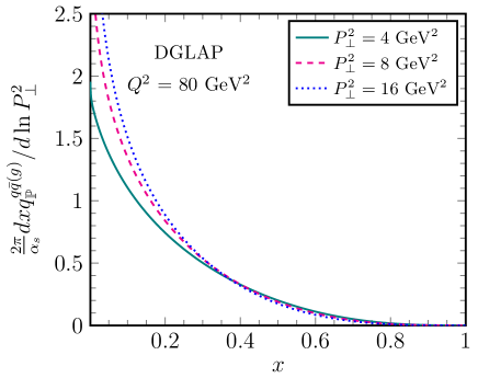
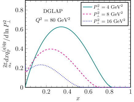
Figure 23: The soft gluon $q\bar{q}(g)$ (left panel) and soft quark $(q)\bar{q}g$ (right panel) contributions to the quark DTMD, cf. Eq. (5), as functions of $x$ for various values of $P_{\perp}^{2}$. As compared to Fig. 22, the distributions are multiplied by a factor $P^{2}_{\perp}/\alpha_{s}(P_{\perp}^{2})$ in order to remove some strong overall dependences upon $P_{\perp}^{2}$, but keep only those introduced by the DGLAP evolution and by the upper limit $z_{\rm max}=1/(1+4P_{\perp}^{2}/Q^{2})$ in the first integral (5). In the case of a soft gluon, we see a rapid rise as $x\to 0$, due to the growth of the gluon DPDF. The contribution involving a soft quark vanishes faster when $x$ is near 1, due to the upper limit $z_{\rm max}$. A factor $S_{\perp}/4\pi^{3}$ has been omitted.

The $(q)\bar{q}g$ piece for $x\ll 1$ can be computed by using the real part of the splitting function $P_{qq}(z)$ in Eq. (6.3) and the asymptotic solution of the quark DPDF in Eq. (168) and we have

$$\frac{{\rm d}xq_{\mathbb{P}}^{(q)\bar{q}g}(x,x_{\mathbb{P}},P_{\perp}^{2})}{{\rm d}\ln P_{\perp}^{2}}\simeq \,\frac{\alpha_{s}(P_{\perp}^{2})}{2\pi}\,\frac{N_{g}\kappa_{g}(0)Q_{s,g}^{2}(Y_{\mathbb{P}})}{3}\,C_{F}\left[2\ln\frac{1}{1\!-\!z_{\max}}-\frac{z_{\max}(z_{\max}+2)}{2}\right]$$

$$\sqrt{\frac{\ln\frac{\alpha_{s}(\mu_{0}^{2})}{\alpha_{s}(P^{2}_{\perp})}}{4\pi bN_{c}\ln\frac{1}{x}}}\,I_{1}\left(\sqrt{\frac{4N_{c}}{\pi b}\ln\frac{\alpha_{s}(\mu_{0}^{2})}{\alpha_{s}(P^{2}_{\perp})}\ln\frac{1}{x}}\right)\quad\mathrm{for}\quad x\ll 1,$$ (173)

where the last factor in the first line is just the integral of the relevant splitting function. This contribution from the soft quark configuration is subleading when compared to the one from the soft gluon configuration in Eq. (171). Finally, we trivially notice that the $(q)\bar{q}g$ piece vanishes due to kinematic constraints for $x\geq z_{\max}$. Once again, these dependences are in agreement with the respective numerical results, as shown in the right plot of Fig. 23. At this level, one can also observe the good agreement between the results for (2+1)–jets in Fig. 23 and, respectively, Fig. 22.

7 Summary and perspectives

In this paper, we have studied the production of two and three jets via coherent diffraction in photon-nucleus interactions at high energy. We have focused on the hard QCD regime where the photon virtuality $Q$ and/or the relative transverse momentum $P_{\perp}$ of two of the produced jets is much larger than the saturation momentum $Q_{s}$ of the nuclear target. The relevant value of $Q_{s}$ is evaluated at the rapidity gap $Y_{\mathbb{P}}$ and thus includes the high-energy evolution of the gluon distribution in the Pomeron. We have shown that, despite the presence of hard scales, the dominant contributions at large $Q^{2}$ and/or large $P_{\perp}^{2}$ — the leading twist contributions — come from relatively large partonic fluctuations of the virtual photon, with a typical transverse size $R\sim 1/Q_{s}$. Such large configurations avoid the colour transparency of small colour dipoles and thus allow for strong scattering in the vicinity of the black disk limit. In turn, strong scattering is favoured by the elastic nature of the diffractive processes.

In the case of exclusive dijets, the partonic configurations which matter at leading twist (and to leading order) are quark-antiquark fluctuations of the virtual photon, which are very asymmetric: one of the quarks (the “aligned jet”) carries most of the longitudinal momentum of the virtual photon, while the other quark is soft, with a longitudinal momentum fraction $\vartheta_{1}\sim Q_{s}^{2}/Q^{2}\ll 1$. Such typical configurations scatter off the saturated gluons in the target wavefunction and thus acquire transverse momenta of order $Q_{s}$. They provide a leading-twist contribution to diffractive SIDIS, in which the measured jet has transverse momentum of order $Q_{s}$.

In the case of three-jet final states, one of the partons (quark, antiquark, or gluon) must be soft ($\vartheta_{1}\sim Q_{s}^{2}/Q^{2}\ll 1$) and semi-hard ($K_{\perp}\sim Q_{s}$), for the overall system to scatter strongly. Yet, the two other jets can be hard ($P_{\perp}\gg Q_{s}$) and nearly back-to-back in the transverse plane. These asymmetric, “(2+1)–jet”, configurations provide the dominant contribution to the diffractive production of a pair of hard jets, despite the fact that they are formally suppressed by a power of the QCD coupling: at large $P_{\perp}\gg Q_{s}$, this suppression is more than compensated by the fact that the respective cross-section is of leading-twist order, i.e. it only falls like $1/P_{\perp}^{4}$ (to be compared with $1/P_{\perp}^{6}$ for hard exclusive dijets).

In all cases, that is, for both exclusive dijets and for diffractive (2+1)–jets, we found that the respective leading twist contributions admit diffractive TMD factorisation. In practice, this means that the soft parton from the wavefunction of the virtual photon can be reinterpreted as a constituent of the target — more precisely, of the Pomeron —, with a transverse-momentum dependent parton distribution which physically represents the unintegrated quark distribution of the Pomeron. In the case of exclusive dijets, this factorisation is most naturally formulated for diffractive SIDIS and involves the quark diffractive TMD, as originally pointed out in Hatta:2022lzj . For diffractive (2+1)–jets, we meet both the quark and the gluon diffractive TMDs, corresponding to the different possibilities for the soft parton. The case of (2+1)–jets with a soft gluon has been studied earlier Iancu:2022lcw ; Iancu:2021rup and we include here the corresponding results, for completeness (see Eqs. (59)–(62)). Our main new result in this paper is the extension of this factorisation to the case of diffractive (2+1)–jets with a soft quark, together with an explicit proof of the universality of the quark DTMD: indeed, we find exactly the same result for the latter in the case of exclusive dijets (see Eqs. (33)–(34)) and for the three contributions to the cross-section for diffractive (2+1)–jets with a soft quark (cf. Eqs. (121)–(127)).

The colour-dipole approach to the virtual photon wavefunction supplemented with the CGC description of the dense nuclear target provides first principles estimates for the quark and gluon diffractive TMDs — valid at leading order in the QCD running coupling, of course. A main common characteristic of these LO results is the fact that both the quark and the gluon DTMD have support at relatively low transverse momenta, $K_{\perp}\lesssim\tilde{Q}_{s}(x,Y_{\mathbb{P}})$, with $\tilde{Q}_{s}(x,Y_{\mathbb{P}})$ the effective saturation momentum introduced in Eq. (48). This strongly suggests that, due to the fact that it is a colour-singlet, the Pomeron fluctutation of the target is built with quarks and gluons at saturation. As discussed in Sect. 2.5, parton saturation in the Pomeron wavefunction is dual to strong elastic scattering between an external dipole and the target.

Another distinctive feature of our LO results for the quark and gluon TMDs is the fact that they apply for generic values of $x$ (the longitudinal momentum fraction of the measured parton w.r.t. the Pomeron), and not only at small $x$, as is the case for the gluon TMDs which emerge from CGC studies of inclusive scattering Dominguez:2011wm . This makes it possible to use our tree-level results in order to initiate the DGLAP evolution at transverse momenta of the order of $Q_{s}$. Moreover, despite the fact that we often refer to them as “tree-level”, our LO approximations for the quark and gluon TMDs generally include the high-energy BK/JIMWLK evolution Balitsky:1995ub ; Kovchegov:1999yj ; JalilianMarian:1997jx ; JalilianMarian:1997gr ; Kovner:2000pt ; Weigert:2000gi ; Iancu:2000hn ; Iancu:2001ad ; Ferreiro:2001qy with increasing $Y_{\mathbb{P}}$. These “tree-level” results are studied in extenso (via both analytic approximations and numerical solutions) in Sect. 6.1.

By integrating the (tree-level) quark and gluon DTMDs over their transverse momentum argument $K_{\perp}^{2}$ up to the hard resolution scale ($Q^{2}$ or $P_{\perp}^{2}$), one deduces LO approximations for the diffractive PDFs, which control more inclusive cross-sections, like the diffractive structure function. In the context of collinear factorisation, the DPDFs are known to obey the DGLAP equations describing their evolution with increasing the resolution scale. So, it is natural to ask: can one see a similar evolution emerging from the dipole picture ? The calculation of (2+1)–jets gives us the possibility to answer this question: after integrating out two of the final jets (one soft and one hard), one finds a contribution to the cross-section for measuring the other hard jet, which has the right kinematics to encode the DGLAP evolution. And indeed, in Sect. 5 we find that the leading-twist piece of this contribution takes the form of one step in the DGLAP evolution of the LO cross-section for SIDIS in Sect. 2. This is interesting from at least two perspectives. First, it demonstrates the emergence of the DGLAP evolution of the target wavefunction via quantum calculations at the level of the projectile. Second, it suggests that the diffractive TMD factorisation that was established here and in the previous papers Iancu:2022lcw ; Iancu:2021rup ; Hatta:2022lzj at leading order may remain valid after adding quantum corrections.

Our study of the emergence of the DGLAP evolution from the colour dipole picture is still incomplete — for instance, we have not computed the virtual corrections — and it would be interesting to complete this study and also extend it to the inclusive cross-sections which are known to admit TMD factorisation when computed in the dipole picture at leading order Dominguez:2011wm .

The analysis in Sect. 5 also suggests that the natural matching between the tree-level results for the TMDs and the DGLAP equations for the PDFs consists in using the results for the former as source terms in the latter. Using this strategy, in Sect. 6.3 we have presented numerical solutions to the DGLAP equations for the quark and gluon diffractive PDFs. By comparing with the respective tree-level approximations in Sect. 6.2, one can better appreciate both the effects of the DGLAP evolution and the influence of the tree-level results on the DGLAP solutions. As a simple application, in Sect. 6.4 we have used the DGLAP solutions for the quark DPDF to compute the diffractive structure function. Our results are qualitatively consistent with previous calculations for the case of a proton target Golec-Biernat:2001gyl , but they show an interesting twist — a substantial reduction in the effects of the DGLAP evolution — when the target is a large nucleus. This effect can be attributed to the importance of the running coupling corrections during the early stages of the DGLAP evolution.

Another intriguing result which emerges from our calculations is the lack of angular correlations between the two transverse momenta which control diffractive (2+1)–jet production: the relative momentum $\bm{P}$ of the hard dijets and their imbalance $\bm{K}$. Such correlations were systematically found in the literature, in cases where the imbalance $\bm{K}$ is caused by a net momentum transfer between the produced jets and the target. This refers both to inclusive dijets (where the angular correlations measure a tensorial component of the WW gluon TMD  Metz:2011wb ; Dominguez:2011br ; Iancu:2013dta ; Dumitru:2015gaa ; Marquet:2017xwy ; Dumitru:2018kuw ) and to exclusive dijets (where they probe the elliptic gluon Wigner distribution Altinoluk:2015dpi ; Hatta:2016dxp ; Hagiwara:2017fye ; Mantysaari:2019csc ; Salazar:2019ncp ; Mantysaari:2019hkq ; Hatta:2021jcd ). In our calculations, we systematically neglected the net momentum transferred via the elastic scattering, since this is tiny ($\Delta_{\perp}\sim 30$ MeV) and in any case much smaller than the recoil $K_{\perp}$ of the semi-hard jet. The (2+1)–jet cross-section depends upon both $\bm{P}$ and $\bm{K}$ and we see no a priori reason to exclude tensorial components in the diffractive TMDs. Yet, we found no trace of them in our final results. This is particularly surprising since our intermediate calculations involve rather complex tensorial structures built with these two vectors (notably, for the interference between the two channels for (2+1)–jets with a soft quark), yet they leave no imprint on the cross-section. It would be interesting to understand if the absence of angular correlations for diffractive jets is a generic feature and if it has a fundamental explanation.

Finally, it would be interesting to consider the phenomenological implications of our new results in more detail. In a recent paper Iancu:2023lel , some of us considered 2+1 diffractive dijets with a soft gluon in the context of ultra-peripheral nucleus-nucleus collisions at the LHC. It would clearly be interesting to add the contributions from the other channels, which involve a soft quark. More generally, one should systematically study the consequences of our results for the future phenomenology at the Electron Ion Collider Accardi:2012qut ; Aschenauer:2017jsk ; AbdulKhalek:2022hcn . This also requires some theoretical refinements, like a better treatment of the final states (by constructing real jets, or including parton fragmentation into hadrons) and a study of the impact of additional effects, like the Sudakov corrections Mueller:2013wwa and the soft gluon radiation in the initial and final states (which represents an additional source of angular correlations) Hatta:2021jcd ; Shao:2024nor .

Appendix A Longitudinal sector

In this Appendix we would like to study the case of a longitudinally polarised virtual photon $\gamma^{*}_{L}$. The steps to be followed are very similar to those in the transverse photon case which has been explicitly worked out in the main text, hence we shall only present the most relevant expressions and results. The only technical change, which one must implement in order to go from the transverse to the longitudinal sector, consists of the replacement

$$\varphi^{ij}(\vartheta,\lambda)k^{j}\longrightarrow 2\vartheta(1-\vartheta)Q$$ (174)

in the $\gamma^{*}\to q\bar{q}$ vertex. Let us see how this modifies the various contributions to the cross sections of interest.

A.1 The $q\bar{q}$ component

The probability amplitude (the analog of Eqs. (7) and (11)) reads

$$\psi^{L}_{\lambda_{1}\lambda_{2}}(\vartheta_{1},\bm{k}_{1})=\frac{\delta_{\lambda_{1}\lambda_{2}}}{\sqrt{{2q^{+}}}}\frac{ee_{f}}{(2\pi)^{3}}\,\frac{Q}{E_{q}+E_{\bar{q}}-E_{\gamma}}=\delta_{\lambda_{1}\lambda_{2}}\,\sqrt{\frac{q^{+}}{2}}\,\frac{ee_{f}}{(2\pi)^{3}}\,\frac{2\sqrt{\vartheta_{1}(1-\vartheta_{1})}\,\bar{Q}}{k_{1\perp}^{2}+\bar{Q}^{2}}.$$ (175)

The transformation to coordinate space is achieved via the replacement (the analog of Eq. (12))

$$\frac{\bar{Q}}{k_{1\perp}^{2}+\bar{Q}^{2}}\to\frac{1}{2\pi}\,\bar{Q}K_{0}(\bar{Q}R).$$ (176)

Including the diffractive scattering and performing the inverse Fourier transform leads to (the analog of Eq. (20))

$$\psi^{L,D}_{\lambda_{1}\lambda_{2}}(\vartheta_{1},\bm{k}_{1})=-\delta_{\lambda_{1}\lambda_{2}}\,\sqrt{\frac{q^{+}}{2}}\,\frac{ee_{f}}{(2\pi)^{3}}\,2\sqrt{\vartheta_{1}(1-\vartheta_{1})}\,\frac{\mathcal{Q}_{L}(\bar{Q},k_{1\perp},Y_{\mathbb{P}})}{\bar{Q}},$$ (177)

where we have defined the dimensionless scalar quantity (the analog of Eq. (21))

$$\mathcal{Q}_{L}(\bar{Q},K_{\perp},Y_{\mathbb{P}})\equiv\bar{Q}^{2}\int{\rm d}R\,R\,J_{0}(K_{\perp}R)\,K_{0}(\bar{Q}R)\,\mathcal{T}(R,Y_{\mathbb{P}}).$$ (178)

We finally arrive at the differential cross section (the analog of Eq. (23)

$$\frac{{\rm d}\sigma^{\gamma_{\scriptscriptstyle L}^{*}A\rightarrow q\bar{q}A}}{{\rm d}\vartheta_{1}\,{\rm d}^{2}\bm{K}}=\frac{2S_{\perp}\alpha_{\rm em}N_{c}}{\pi^{2}}\left(\sum e_{f}^{2}\right)\left[\vartheta_{1}(1-\vartheta_{1})\right]\frac{|\mathcal{Q}_{L}(\bar{Q},K_{\perp},Y_{\mathbb{P}})|^{2}}{\bar{Q}^{2}},$$ (179)

which, for a fixed value of the rapidity gap $Y_{\mathbb{P}}$ or, equivalently, of $\beta$, becomes (the analog of Eq. (31))

$$\frac{{\rm d}\sigma^{\gamma_{L}^{*}A\rightarrow q\bar{q}A}}{{\rm d}\ln(1/\beta)\,{\rm d}^{2}\bm{K}}=\frac{4S_{\perp}\alpha_{\rm em}N_{c}}{\pi^{2}}\left(\sum e_{f}^{2}\right)\,\frac{1}{Q^{2}}\,\frac{\frac{\mathcal{M}^{2}}{Q^{2}}}{\sqrt{1-\frac{4\mathcal{M}^{2}}{Q^{2}}}}\,\frac{[\mathcal{Q}_{L}(\mathcal{M},K_{\perp},Y_{\mathbb{P}})]^{2}}{1-\beta},$$ (180)

where $\mathcal{M}^{2}=[\beta/(1-\beta)]K_{\perp}^{2}$. We recall that the change of variables from $\vartheta_{1}$ to $\beta$ has replaced $\vartheta_{1}(1-\vartheta_{1})\to\mathcal{M}^{2}/Q^{2}$ and hence $\bar{Q}\to\mathcal{M}$, cf. Eq. (30). It is furthermore understood that $K_{\perp}\leq K_{\max}$ with the upper limit $K_{\max}^{2}=(1-\beta)Q^{2}/4\beta$ from Eq. (29).

By inspection of Eq. (180), it is apparent that this quantity is of higher-twist order — it starts at twist-4 order, i.e. it decays like $1/Q^{4}$ in the high $Q^{2}$ limit—, hence it brings no contribution to the quark diffractive TMD. Clearly, this suppression should be attributed to the factor $\vartheta_{1}(1-\vartheta_{1})$ in the r.h.s. of Eq. (179), which is the splitting function for the decay $\gamma^{*}_{L}\to q\bar{q}$ of the longitudinal photon, cf. Eq. (128). This factor is much smaller than one for the asymmetric $q\bar{q}$ configurations. Yet, as observed in Ref. Golec-Biernat:2001gyl , the longitudinal sector gives the dominant contribution to the diffractive structure function in the limit $\beta\to 1$, since it remains finite in that limit, unlike the leading-twist contribution of the transverse cross section, which vanishes like $1-x$, cf. Eqs. (53) and (55).

In order to demonstrate this and to gain more insight in the physical content of Eq. (180), let us estimate this cross-section in two limiting regimes: for small and respectively large transverse momenta $K_{\perp}$. The discussion of $\mathcal{Q}_{L}$ in these limits is similar to that of the quantity $\mathcal{Q}_{\mathbb{P}}$ in Sect. 2.5, except for the fact that the variable $x$ is now replaced by $\beta$. In particular, $R_{\max}^{2}\sim(1-\beta)/K_{\perp}^{2}$ and the effective saturation momentum is $\tilde{Q}_{s}(\beta,Y_{\mathbb{P}})=\sqrt{1-\beta}\,Q_{s}(Y_{\mathbb{P}})$. For the purpose of parametric estimates, one can replace $J_{0}(K_{\perp}R)\,K_{0}(\mathcal{M}R)\sim\Theta(R_{\max}-R)$.

(i) When $K_{\perp}\!\gg\!\sqrt{(1-\beta)}\,Q_{s}(Y_{\mathbb{P}})$ the scattering is weak and we have (the analog of Eq. (2.5))

$$\mathcal{Q}_{L}\sim\mathcal{M}^{2}Q_{s}^{2}R_{\max}^{4}\sim\beta\,(1-\beta)\frac{Q_{s}^{2}(Y_{\mathbb{P}})}{K_{\perp}^{2}}\qquad\mathrm{for}\qquad K_{\perp}\gg\tilde{Q}_{s}(\beta,Y_{\mathbb{P}}),$$ (181)

where logarithmic factors have been neglected.

(ii) When $K_{\perp}\!\ll\!\sqrt{(1-\beta)}\,Q_{s}(Y_{\mathbb{P}})$, the integration over $R$ is dominated by large dipoles which scatter strongly off the target and gives (the analog of Eq. (2.5))

$$\mathcal{Q}_{L}\sim\mathcal{M}^{2}R_{\max}^{2}\sim\beta\qquad\mathrm{for}\qquad K_{\perp}\!\ll\!\ \tilde{Q}_{s}(\beta,Y_{\mathbb{P}}).$$ (182)

For completeness, we point out that one can perform a precise calculation for case (i) in the MV model (similar to the one in Appendix B), while the above estimate in case (ii) is in fact equal to the exact result.

The above results can be conveniently summarised in the following, piece-wise approximation:

$$\,\frac{\mathcal{M}^{2}}{Q^{2}}\,\frac{[\mathcal{Q}_{L}]^{2}}{1-\beta}\,\simeq\,\beta^{3}\begin{cases}\displaystyle{\,\frac{Q_{s}^{4}(Y_{\mathbb{P}})}{Q^{2}K_{\perp}^{2}}}&\quad{\rm for}\quad\tilde{Q}_{s}(\beta,Y_{\mathbb{P}})\ll K_{\perp}\leq K_{\max}\\[11.38092pt] \displaystyle{\,\frac{1}{(1-\beta)^{2}}\,\frac{K_{\perp}^{2}}{Q^{2}}}&\quad{\rm for}\quad K_{\perp}\ll\tilde{Q}_{s}(\beta,Y_{\mathbb{P}})\,.\end{cases}$$ (183)

This shows that the cross-section (179) is peaked at $K_{\perp}\sim\tilde{Q}_{s}(\beta,Y_{\mathbb{P}})$, but unlike in the transverse sector, the bulk of the distribution is located above this peak, in the slowly decaying tail at larger transverse momenta $K_{\perp}\gg\tilde{Q}_{s}(\beta,Y_{\mathbb{P}})$. This becomes clear when integrating over $K_{\perp}$, to deduce the contribution of the longitudinal sector to the diffractive structure function $F_{2}^{D(3)}$ (cf. Eq. (2)). Using the estimate in Eq. (183), one can easily check that the dominant contribution comes from high-momentum tail $\propto 1/K_{\perp}^{2}$, since the respective integral over $K_{\perp}^{2}$ yields a large transverse logarithm $\ln[Q^{2}/Q_{s}^{2}(Y_{\mathbb{P}})]$. To leading logarithmic accuracy, one can assume that $K_{\perp}\ll K_{\max}$ and thus approximate the square root in the denominator of (180) by unity. This argument also shows that dominant contribution comes from aligned jet configurations: $\vartheta_{1}(1-\vartheta_{1})=\mathcal{M}^{2}/Q^{2}\ll 1$. One thus finds

$$\frac{{\rm d}\sigma^{\gamma_{L}^{*}A\rightarrow q\bar{q}A}}{{\rm d}\ln(1/\beta)}\propto S_{\perp}\frac{4\beta^{3}\alpha_{em}N_{c}}{\pi}\left(\sum e_{f}^{2}\right)\frac{Q_{s}^{4}(Y_{\mathbb{P}})}{Q^{4}}\,\ln\frac{Q^{2}}{4\beta Q_{s}^{2}(Y_{\mathbb{P}})}\,,$$ (184)

where the logarithm has been generated as $\ln\big{[}K_{\max}^{2}/\tilde{Q}_{s}^{2}\big{]}=\ln\big{[}{Q^{2}}/{4\beta Q_{s}^{2}}\big{]}$. Notice that the factor $1-\beta$ has cancelled in the ratio $K_{\max}^{2}/\tilde{Q}_{s}^{2}$, that is, in the argument of the logarithm. The final result in Eq. (184) does not vanish in the limit $\beta\to 1$, where it even dominates over the leading-twist contribution of the transverse sector, which vanishes there, cf. Eq. (55). A similar observation was made in Golec-Biernat:2001gyl . However, outside this limit, the longitudinal contribution (184) is of twist-4 order and thus is strongly suppressed at high $Q^{2}\gg Q_{s}^{2}(Y_{\mathbb{P}})$ compared to the LT result in Eqs. (53) and (55). The derivation of Eq. (184) relies on the high momentum behavior in Eq. (183) which is valid for a scattering amplitude which is given by the GBW model. When using the MV model the precise high momentum behavior can be inferred from Eqs. (207) and (208) in Appendix B. Eventually, this results in an even stronger logarithmic dependence, namely the longitudinal cross section in Eq. (184) becomes proportional to $\ln^{3}(Q^{2}/4\beta^{2}\Lambda^{2})-\ln^{3}(Q_{s}^{2}/\beta\Lambda^{2})$.

A.2 The $q\bar{q}g$ component

As explained in Sect. 3, we consider $q\bar{q}g$ configurations which are asymmetric in the sense that the (final) quark is both soft and semi-hard, whereas the (final) antiquark is hard and carries a large fraction of the photon longitudinal momentum. Because of this asymmetry, gluon emissions from the quark and, respectively, the antiquark lead to very different $q\bar{q}g$ states. This difference has also consequences in the case where the incoming photon has longitudinal polarisation, as we now explain.

(i) Gluon emission from the antiquark.

The total amplitude after taking into account the gluon emission both before and after the scattering is (the analog of (80))

$$\Psi^{L,m}_{\lambda_{1}\lambda_{2}\,(\bar{q})}\simeq-\,\delta_{\lambda_{1}\lambda_{2}}\,\frac{ee_{f}gq^{+}}{(2\pi)^{6}}\,\frac{\vartheta_{1}}{\sqrt{\vartheta_{3}}}\,\frac{Q}{k_{1\perp}^{2}+\mathcal{M}^{2}}\,\frac{\tau^{mn}(0,\vartheta_{2},\lambda_{1})P^{n}}{P_{\perp}^{2}},$$ (185)

valid for $\vartheta_{1}\ll 1$ and $k_{1\perp}\ll P_{\perp}$. Taking the Fourier transform w.r.t. the semi-hard momentum $\bm{k}_{1}$, inserting the diffractive scattering and performing the inverse Fourier transform we get (the analog of (89))

$$\Psi^{L,m,D}_{\lambda_{1}\lambda_{2}(\bar{q})}\simeq\,\delta_{\lambda_{1}\lambda_{2}}\,\frac{ee_{f}gq^{+}}{(2\pi)^{6}}\,\frac{\vartheta_{1}}{\sqrt{\vartheta_{3}}}\,\frac{Q}{\mathcal{M}}\frac{\tau^{mn}(0,\vartheta_{2},\lambda_{1})P^{n}}{P_{\perp}^{2}}\,\frac{\mathcal{Q}_{L}(\mathcal{M},K_{\perp},Y_{\mathbb{P}})}{\mathcal{M}}.$$ (186)

Recalling the definition in Eq. (72) we have

$$\sum_{m,\lambda}\tau^{mn}(0,\vartheta,\lambda)\tau^{mr*}(0,\vartheta,\lambda)=4(1+\vartheta^{2})\delta^{nr},$$ (187)

which allows us to calculate the magnitude squared of Eq. (186) and arrive at the cross section

$$\frac{{\rm d}\sigma_{(\bar{q}\bar{q})}^{\gamma_{\scriptscriptstyle L}^{*}A\rightarrow q\bar{q}gA}}{{\rm d}\vartheta_{1}{\rm d}\vartheta_{2}{\rm d}\vartheta_{3}\,{\rm d}^{2}\bm{P}{\rm d}^{2}\bm{K}}=\frac{S_{\perp}\alpha_{\rm em}N_{c}}{\pi^{4}}\left(\sum e_{f}^{2}\right)\delta_{\vartheta}\,\frac{\alpha_{s}C_{F}\tilde{Q}^{2}}{P_{\perp}^{2}(P_{\perp}^{2}+\tilde{Q}^{2})}\,\frac{\vartheta_{1}(1+\vartheta_{2}^{2})}{\vartheta_{3}}\,\frac{\big{|}\mathcal{Q}_{L}(\mathcal{M},K_{\perp},Y_{\mathbb{P}})\big{|}^{2}}{\mathcal{M}^{2}},$$ (188)

where we have also used Eq. (79). We immediately see that this longitudinal cross section is power suppressed when compared to the corresponding transverse one in Eq. (107) due to the presence of an extra factor $\vartheta_{1}\sim K_{\perp}^{2}/Q^{2}\ll 1$. Physically, this suppression is related to the fact that the original $q\bar{q}$ pair created by the decay of the longitudinal virtual photon is very asymmetric.

(ii) Gluon emission from the quark.

The respective amplitude is dominated by the diagram in which the gluon is emitted before the scattering and reads (the analog of (98))

$$\Psi^{Lm}_{\lambda_{1}\lambda_{2}(q)}\simeq-\,\delta_{\lambda_{1}\lambda_{2}}\,\frac{ee_{f}gq^{+}}{(2\pi)^{6}}\,\frac{\sqrt{\vartheta_{2}}}{\vartheta_{3}}\,\frac{\tilde{Q}}{P_{\perp}^{2}+\tilde{Q}^{2}}\,\frac{\tau^{mn*}(\vartheta_{2},0,\lambda_{1})k_{1}^{n}}{k_{1\perp}^{2}+\mathcal{M}^{2}},$$ (189)

valid for $\vartheta_{1}\ll 1$ and $k_{1\perp}\ll P_{\perp}$. We take the Fourier transform w.r.t. the semi-hard momentum $\bm{k}_{1}$, insert the diffractive scattering and perform the inverse Fourier transform to get (the analog of (102))

$$\Psi^{Lm,D}_{\lambda_{1}\lambda_{2}(q)}\simeq-\delta_{\lambda_{1}\lambda_{2}}\,\frac{ee_{f}gq^{+}}{(2\pi)^{6}}\,\frac{\sqrt{\vartheta_{2}}}{\vartheta_{3}}\,\frac{\tilde{Q}}{P_{\perp}^{2}+\tilde{Q}^{2}}\,\frac{\tau^{mn*}(\vartheta_{2},0,\lambda_{1})K^{n}}{K_{\perp}}\,\frac{\mathcal{Q}_{\mathbb{P}}(\mathcal{M},K_{\perp},Y_{\mathbb{P}})}{\mathcal{M}}.$$ (190)

Using

$$\sum_{m,\lambda}\tau^{mn*}(\vartheta,0,\lambda)\tau^{mr}(\vartheta,0,\lambda)=4(1-\vartheta)^{2}\delta^{nr},$$ (191)

we obtain the cross section

$$\frac{{\rm d}\sigma_{(qq)}^{\gamma_{\scriptscriptstyle L}^{*}A\rightarrow q\bar{q}gA}}{{\rm d}\vartheta_{1}{\rm d}\vartheta_{2}{\rm d}\vartheta_{3}\,{\rm d}^{2}\bm{P}{\rm d}^{2}\bm{K}}=\frac{S_{\perp}\alpha_{\rm em}N_{c}}{\pi^{4}}\left(\sum e_{f}^{2}\right)\delta_{\vartheta}\,\frac{\alpha_{s}C_{F}\tilde{Q}^{2}}{(P_{\perp}^{2}+\tilde{Q}^{2})^{2}}\,\vartheta_{2}\,\frac{\big{|}\mathcal{Q}_{\mathbb{P}}(\mathcal{M},K_{\perp},Y_{\mathbb{P}})\big{|}^{2}}{\mathcal{M}^{2}},$$ (192)

which is of the same order with the corresponding transverse cross section in Eq. (110). In fact, we can also express this result in terms of the quark DTMD introduced in Eq. (34); that is, Eq. (192) admits TMD factorisation at the hard dijet level, similarly to Eq. (123). This factorised form is exhibited in Eqs. (129)–(130) in the main text.

Since one of the two amplitudes (that where the gluon is emitted from the antiquark) is power-suppressed by the factor $\vartheta_{1}\sim K_{\perp}^{2}/Q^{2}\ll 1$, the same is also true for the interference term, so we shall not attempt to compute the latter.

Appendix B Quark and gluon diffractive TMDs in the single scattering approximation

Here we shall present exact calculations of $\mathcal{Q}_{\mathbb{P}}$ in Eq. (35), $\mathcal{Q}_{L}$ in Eq. (178), and $\mathcal{G}_{\mathbb{P}}$ in Eq. (63), within the context of the MV model and in the regime of weak scattering. The results to be obtained here are referred at several places in the main text. In particular, we shall demonstrate the power suppression of the cross-section for exclusive dijet production at large $K_{\perp}\gg Q_{s}(Y_{\mathbb{P}})$.

For the present purposes, the dipole scattering amplitude $\mathcal{T}(R)$ is given by the single scattering approximation to the MV model, meaning by the exponent of Eq. (43). This is a legitimate approximation when at least one of the two scales $K_{\perp}$ and $\mathcal{M}$ is much larger than the saturation momentum $Q_{s}$, i.e. when $\max\{K_{\perp},\mathcal{M}\}\gg Q_{s}$. The smaller of these two scales does not need to satisfy any constraint w.r.t. $Q_{s}$. Due to the presence of the Bessel functions the integration has support only for dipoles with size such that $R\lesssim\min\{1/K_{\perp},1/\mathcal{M}\}\ll 1/Q_{s}$, thus justifying the use of the single scattering approximation. We shall not make any assumptions regarding the relation between the scales $\mathcal{M}$ and $K_{\perp}$ and therefore no simplification can be done to any of the two Bessel functions.

(i) Quark DTMD.

We have (cf. Eq. (35))

$$\mathcal{Q}_{\mathbb{P}}=\frac{Q_{A}^{2}\mathcal{M}^{2}}{4}\int_{0}^{\infty}{\rm d}R\,R^{3}J_{1}(K_{\perp}R)K_{1}(\mathcal{M}R)\left(\ln\frac{K_{\perp}^{2}}{\Lambda^{2}}+\ln\frac{4}{K_{\perp}^{2}R^{2}}\right),$$ (193)

where for our convenience we have split the logarithm of the MV model into two terms. The first logarithm is independent of the variable $R$ and the respective integration is standard, leading to the contribution

$$\mathcal{Q}_{\mathbb{P}}^{(1)}=\frac{2Q_{A}^{2}K_{\perp}\mathcal{M}^{3}}{(K_{\perp}^{2}+\mathcal{M}^{2})^{3}}\,\ln\frac{K_{\perp}^{2}}{\Lambda^{2}}.$$ (194)

The second contribution is more involved because the logarithm depends on $R$ and we shall write it as

$$\mathcal{Q}_{\mathbb{P}}^{(2)}=-\frac{Q_{A}^{2}\mathcal{M}^{2}}{4}\lim_{a\to 0}\frac{{\rm d}}{{\rm d}a}\int_{0}^{\infty}{\rm d}R\,R^{3}\left(\frac{K_{\perp}^{2}R^{2}}{4}\right)^{a}J_{1}(K_{\perp}R)K_{1}(\mathcal{M}R).$$ (195)

Next we expand the Bessel function $J_{1}(K_{\perp}R)$ in a power series to get

$$\mathcal{Q}_{\mathbb{P}}^{(2)}=-\frac{Q_{A}^{2}\mathcal{M}^{2}K_{\perp}}{8}\sum_{n=0}^{\infty}\frac{(-1)^{n}}{n!(n+1)!}\,\lim_{a\to 0}\frac{{\rm d}}{{\rm d}a}\int_{0}^{\infty}{\rm d}R\,R^{4}\left(\frac{K_{\perp}^{2}R^{2}}{4}\right)^{n+a}\!\!K_{1}(\mathcal{M}R)$$ (196)

and a straightforward calculation of the last integral (which is clearly convergent for all the relevant values of $n$ and $a$) leads to

$$\mathcal{Q}_{\mathbb{P}}^{(2)}=-\frac{Q_{A}^{2}K_{\perp}}{\mathcal{M}^{3}}\sum_{n=0}^{\infty}\frac{1}{n!(n+1)!}\left(-\frac{K_{\perp}^{2}}{\mathcal{M}^{2}}\right)^{n}\!\lim_{a\to 0}\frac{{\rm d}}{{\rm d}a}\left[\left(\frac{K_{\perp}^{2}}{\mathcal{M}^{2}}\right)^{a}\!\Gamma(n+2+a)\Gamma(n+3+a)\right].$$ (197)

Differentiating with respect to $a$ and subsequently setting $a=0$ gives

$$\mathcal{Q}_{\mathbb{P}}^{(2)}=-\frac{Q_{A}^{2}K_{\perp}}{\mathcal{M}^{3}}\sum_{n=0}^{\infty}(n+1)(n+2)\!\left(-\frac{K_{\perp}^{2}}{\mathcal{M}^{2}}\right)^{n}\!\left[\ln\frac{K_{\perp}^{2}}{\mathcal{M}^{2}}+\Psi(n+2)+\Psi(n+3)\right],$$ (198)

where $\Psi(n)$ is the logarithmic derivative of $\Gamma(n)$. For $K_{\perp}<\mathcal{M}$ the series is convergent and we obtain

$$\mathcal{Q}_{\mathbb{P}}^{(2)}=\frac{Q_{A}^{2}K_{\perp}\mathcal{M}^{3}}{(K_{\perp}^{2}+\mathcal{M}^{2})^{3}}\,\left[4\ln\frac{K_{\perp}^{2}+\mathcal{M}^{2}}{K_{\perp}\mathcal{M}}+\frac{K_{\perp}^{2}}{\mathcal{M}^{2}}-(5-4\gamma_{\scriptscriptstyle E})\right],$$ (199)

with $\gamma_{\scriptscriptstyle E}\simeq 0.577$ the Euler constant. By analytic continuation, the above gives the correct result for the second contribution to the integration in Eq. (193) for any value of $K_{\perp}$ and $\mathcal{M}$. Putting together Eqs. (194) and (199) we finally arrive at

$$\mathcal{Q}_{\mathbb{P}}=\frac{Q_{A}^{2}K_{\perp}\mathcal{M}^{3}}{(K_{\perp}^{2}+\mathcal{M}^{2})^{3}}\,\left[2\ln\frac{(K_{\perp}^{2}+\mathcal{M}^{2})^{2}}{\mathcal{M}^{2}\Lambda^{2}}+\frac{K_{\perp}^{2}}{\mathcal{M}^{2}}-(5-4\gamma_{\scriptscriptstyle E})\right].$$ (200)

We also notice that the last, constant, term in the square bracket can be neglected, since it is always logarithmically suppressed w.r.t the first term (or even power suppressed w.r.t. the second term when $K_{\perp}$ is much larger than $\mathcal{M}$).

Let us now examine how the above general expression simplifies in the various kinematic regimes as determined by the scales $K_{\perp}$ and $\mathcal{M}$. We recall that at least one of the two must be much larger than $Q_{s}$ for $\eqref{app:QPtot}$ to be valid.

1. When $K_{\perp}\sim\mathcal{M}$ (that is, when $x$ is neither close to 0 nor to 1), the logarithm in the square bracket dominates and to the order of accuracy can be approximated as $\ln K_{\perp}^{2}/\Lambda^{2}$, so that

   $$\mathcal{Q}_{\mathbb{P}}\simeq\frac{2Q_{A}^{2}K_{\perp}\mathcal{M}^{3}}{(K_{\perp}^{2}+\mathcal{M}^{2})^{3}}\,\ln\frac{K_{\perp}^{2}}{\Lambda^{2}}=\mathcal{Q}_{\mathbb{P}}^{(1)}\quad{\rm for}\quad K_{\perp}\sim\mathcal{M}.$$ (201)

   We point out that the prefactor in the above is under control and that in this regime the answer is solely given by the first contribution in Eq. (194). Indeed, the argument of the logarithm in Eq. (199) is of the order of one when $K_{\perp}\sim\mathcal{M}$ and thus the second contribution can be neglected. The above result is in complete agreement with Eq. (A.9) in Iancu:2022lcw .

2. When $K_{\perp}\gg\mathcal{M}$ (that is, when $x\ll 1$), the second term in the square bracket in Eq. (200) is by far the largest and hence

   $$\mathcal{Q}_{\mathbb{P}}\simeq\frac{Q_{A}^{2}\mathcal{M}}{K_{\perp}^{3}}\simeq\frac{\sqrt{x}\,Q_{A}^{2}}{K_{\perp}^{2}}\quad{\rm for}\quad K_{\perp}\gg\mathcal{M}.$$ (202)

   Clearly, this could have been obtained directly by keeping only the first term in the expansion of $K_{1}(\mathcal{M}R)$.

3. When $K_{\perp}\ll\mathcal{M}$ (that is, when $1-x\ll 1$), the logarithm in the square bracket in Eq. (200) is enhanced and we easily find

   $$\mathcal{Q}_{\mathbb{P}}\simeq\frac{2Q_{A}^{2}K_{\perp}}{\mathcal{M}^{3}}\,\ln\frac{\mathcal{M}^{2}}{\Lambda^{2}}\simeq\frac{2(1-x)^{3/2}Q_{A}^{2}}{K_{\perp}^{2}}\,\ln\frac{K_{\perp}^{2}}{(1-x)\Lambda^{2}}\quad{\rm for}\quad K_{\perp}\ll\mathcal{M}.$$ (203)

   In this case the result could have been obtained directly by keeping only the first term in the expansion of $J_{1}(K_{\perp}R)$.

(ii) Hard exclusive dijets.

As a direct application of the above, let us consider the production of a pair of hard dijets with $K_{\perp}\sim\bar{Q}\gg Q_{s}$ via elastic scattering. The cross-section is given by Eq. (22) which, after integrating out a couple of trivial $\delta$–functions, becomes Eq. (23). Notice that the relevant kinematical variables are different w.r.t. the previous discussion: on fixes the longitudinal fraction $\vartheta_{1}$, rather than $\beta$ (which can be computed in terms of $\vartheta_{1}$ and $K_{\perp}$, cf. Eq. (26)). In particular, the effective virtuality is now denoted as $\bar{Q}$, instead of $\mathcal{M}$. Taking into account these minor changes, one finds the following expression for the exclusive dijet cross-section in the hard regime (cf. Eq. (201))

$$\frac{{\rm d}\sigma^{\gamma_{\scriptscriptstyle T}^{*}A\rightarrow q\bar{q}A}}{{\rm d}\vartheta_{1}\,{\rm d}^{2}\bm{K}} \,\simeq\frac{S_{\perp}\alpha_{\rm em}N_{c}}{2\pi^{2}}\left(\sum e_{f}^{2}\right)\left[\vartheta_{1}^{2}+(1-\vartheta_{1})^{2}\right]\frac{4\bar{Q}^{4}K_{\perp}^{2}}{(K_{\perp}^{2}+\bar{Q}^{2})^{6}}\,\left[Q_{A}^{2}\ln\frac{K_{\perp}^{2}}{\Lambda^{2}}\right]^{2}\,.$$ (204)

For large and comparable values of $K_{\perp}$ and $\bar{Q}$, this cross-section decreases like $1/K_{\perp}^{6}$.

(iii) Longitudinal sector.

Following the exact same steps, we can calculate the corresponding quantity $\mathcal{Q}_{L}$, introduced in Eq. (178), in the longitudinal sector. In the single scattering approximation we have

$$\mathcal{Q}_{L}=\frac{Q_{A}^{2}\mathcal{M}^{2}}{4}\int_{0}^{\infty}{\rm d}R\,R^{3}J_{0}(K_{\perp}R)K_{0}(\mathcal{M}R)\ln\frac{4}{R^{2}\Lambda^{2}}$$ (205)

and we obtain the exact result

$$\mathcal{Q}_{L}=\frac{Q_{A}^{2}\mathcal{M}^{2}}{(K_{\perp}^{2}+\mathcal{M}^{2})^{3}}\,\left\{\big{(}\mathcal{M}^{2}-K_{\perp}^{2}\big{)}\left[\ln\frac{(K_{\perp}^{2}+\mathcal{M}^{2})^{2}}{\mathcal{M}^{2}\Lambda^{2}}+2(\gamma_{\scriptscriptstyle E}-1)\right]+2K_{\perp}^{2}\right\}.$$ (206)

To the order of accuracy the constant term $2(\gamma_{\scriptscriptstyle E}-1)$ can always be dropped. When $K_{\perp}\gg\mathcal{M}$ the above reduces to

$$\mathcal{Q}_{L}\simeq-\frac{Q_{A}^{2}\mathcal{M}^{2}}{K_{\perp}^{4}}\,\ln\frac{K_{\perp}^{4}}{\mathcal{M}^{2}\Lambda^{2}}\simeq-\frac{xQ_{A}^{2}}{K_{\perp}^{2}}\,\ln\frac{K_{\perp}^{2}}{x\Lambda^{2}}\quad{\rm for}\quad K_{\perp}\gg\mathcal{M},$$ (207)

whereas for $K_{\perp}\ll\mathcal{M}$ one finds

$$\mathcal{Q}_{L}\simeq\frac{Q_{A}^{2}}{\mathcal{M}^{2}}\,\ln\frac{\mathcal{M}^{2}}{\Lambda^{2}}\simeq\frac{(1-x)Q_{A}^{2}}{K_{\perp}^{2}}\,\ln\frac{K_{\perp}^{2}}{(1-x)\Lambda^{2}}\quad{\rm for}\quad K_{\perp}\gg\mathcal{M}.$$ (208)

(iv) Gluon DTMD.

Finally, we can do the analogous calculation for the amplitude $\mathcal{G}_{\mathbb{P}}$ in Eq. (63) which determines the gluon DTMD. We start with

$$\mathcal{G}_{\mathbb{P}}=\frac{Q_{A,g}^{2}\mkern 1.0mu\mathcal{M}^{2}}{4}\int_{0}^{\infty}{\rm d}R\,R^{3}J_{2}(K_{\perp}R)K_{2}(\mathcal{M}R)\ln\frac{4}{R^{2}\Lambda^{2}},$$ (209)

where $Q_{A,g}^{2}$ is enhanced by a color factor $N_{c}/C_{\scriptscriptstyle F}$ w.r.t. to $Q_{A}^{2}$ introduced in Eq. (43), to arrive at the final exact result

$$\mathcal{G}_{\mathbb{P}}=\frac{Q_{A,g}^{2}K_{\perp}^{2}(K_{\perp}^{2}+3\mathcal{M}^{2})}{(K_{\perp}^{2}+\mathcal{M}^{2})^{3}}\,\bigg{[} \ln\frac{K_{\perp}^{2}+\mathcal{M}^{2}}{\Lambda^{2}}+\frac{(2\gamma_{\scriptscriptstyle E}\!-\!1)K_{\perp}^{2}-6(1\!-\!\gamma_{\scriptscriptstyle E})\mathcal{M}^{2}}{K_{\perp}^{2}+3\mathcal{M}^{2}}$$

$$+\frac{\mathcal{M}^{4}}{K_{\perp}^{2}(K_{\perp}^{2}+3\mathcal{M}^{2})}-\frac{\mathcal{M}^{4}(3K_{\perp}^{2}+\mathcal{M}^{2})}{K_{\perp}^{4}(K_{\perp}^{2}+3\mathcal{M}^{2})}\ln\frac{K_{\perp}^{2}+\mathcal{M}^{2}}{\mathcal{M}^{2}}\bigg{]}.$$ (210)

Independently of the order between the scales $K_{\perp}$ and $\mathcal{M}$, the first term dominates the sum in the square bracket (notice that when $\mathcal{M}\gg K_{\perp}$ the last two terms give a combined contribution of the order of one although each of them is of the order of $\mathcal{M}^{2}/K_{\perp}^{2}\gg 1$) and therefore we can write to logarithmic accuracy

$$\mathcal{G}_{\mathbb{P}}\simeq\frac{Q_{A,g}^{2}K_{\perp}^{2}(K_{\perp}^{2}+3\mathcal{M}^{2})}{(K_{\perp}^{2}+\mathcal{M}^{2})^{3}}\,\ln\frac{K_{\perp}^{2}+\mathcal{M}^{2}}{\Lambda^{2}}\quad{\rm for\,\,any}\quad K_{\perp},\mathcal{M}.$$ (211)

The above is in exact agreement with (the second line in) Eq. (5.8) in Iancu:2022lcw .

Appendix C Instantaneous interaction terms

In this Appendix, we will show that when studying 2+1 jet production, where the source of the semi-hard jet is a quark or an antiquark, the diagrams involving instantaneous interactions are subleading. This should be contrasted to the case of a semi-hard gluonic jet, in which the contribution of instantaneous terms is of the same order as the regular ones and is in fact crucial for obtaining the correct wavefunction of the gluon-gluon dipole.

(i) Gluon emission from the antiquark in the transverse sector.

From Iancu:2022gpw , one can infer that the exact probability amplitude of interest reads

$$\Psi^{ij,{\rm inst}}_{\lambda_{1}\lambda_{2}\,(\bar{q})}=\delta_{\lambda_{1}\lambda_{2}}\,\frac{ee_{f}g}{4(2\pi)^{6}}\,\frac{1}{\sqrt{\vartheta_{3}}(1-\vartheta_{1})}\,\frac{\bar{\varphi}^{ij}(\lambda_{1})}{E_{q}+E_{\bar{q}}+E_{g}-E_{\gamma}},$$ (212)

where

$$\bar{\varphi}^{ij}(\lambda)\equiv\delta^{ij}+2i\lambda\varepsilon^{ij}.$$ (213)

The photon decay and the gluon emission happen at the same time and this leads to various differences w.r.t. to the regular terms. First, when comparing to Eq. (70), we observe that now the intermediate energy denominator $E_{q}+E_{\bar{q}^{\prime}}-E_{\gamma}$ is absent. Second, both the electromagnetic and the QCD vertex are independent of the momenta. Finally, it is clear that the scattering occurs after the gluon emission, which means that there is only diagram, the one in which the trijet state crosses the nuclear shockwave.

One should be careful enough not to compare Eq. (212) with Eq. (70), but with the total probability amplitude in Eq. (80). Indeed, when one combines Eqs. (70) and (75), the aforementioned energy denominator $E_{q}+E_{\bar{q}^{\prime}}-E_{\gamma}$ which involves semi-hard transverse momenta cancels, and the new denominator which appears is much harder, cf. Eq. (77). Hence, the total amplitude is much smaller than the two individual contributions and it is not a priori clear that it will me much larger than the instantaneous term. Still, by making use of Eqs. (3.2) and (79), we can write the instantaneous term as

$$\Psi^{ij,{\rm inst}}_{\lambda_{1}\lambda_{2}\,(\bar{q})}\simeq\delta_{\lambda_{1}\lambda_{2}}\,\frac{ee_{f}gq^{+}}{2(2\pi)^{6}}\,\frac{\vartheta_{1}}{\sqrt{\vartheta_{3}}}\,\frac{\bar{\varphi}^{ij}(\lambda_{1})}{k_{1\perp}^{2}+\mathcal{M}^{2}}$$ (214)

and it is straightforward to check that the above is power suppressed w.r.t. to the regular contribution in Eq. (80) when $\vartheta_{1}\ll k_{1\perp}/P_{\perp}$.

(ii) Gluon emission from the quark in the transverse sector.

As we have already seen in the analysis of the regular terms, the probability amplitude with gluon emission from the quark can be obtained from the one with gluon emission from the antiquark by changing the sign, taking the complex conjugate and letting $1\leftrightarrow 2$. Then Eq. (212) changes to

$$\Psi^{ij,{\rm inst}}_{\lambda_{1}\lambda_{2}\,(q)}=-\delta_{\lambda_{1}\lambda_{2}}\,\frac{ee_{f}g}{4(2\pi)^{6}}\,\frac{1}{\sqrt{\vartheta_{3}}(1-\vartheta_{2})}\,\frac{\bar{\varphi}^{ij*}(\lambda_{1})}{E_{q}+E_{\bar{q}}+E_{g}-E_{\gamma}},$$ (215)

and using Eq. (97) we obtain

$$\Psi^{ij,{\rm inst}}_{\lambda_{1}\lambda_{2}\,(\bar{q})}\simeq-\delta_{\lambda_{1}\lambda_{2}}\,\frac{ee_{f}gq^{+}}{2(2\pi)^{6}}\,\frac{\vartheta_{1}}{\vartheta_{3}^{3/2}}\,\frac{\bar{\varphi}^{ij*}(\lambda_{1})}{k_{1\perp}^{2}+\mathcal{M}^{2}}.$$ (216)

Again, the above is power suppressed when compared to Eq. (98) for $\vartheta_{1}\ll k_{1\perp}/P_{\perp}$.

Appendix D Details on 2+1 jet contributions to diffractive SIDIS

In this Appendix, we shall compute in detail the contributions of 2+1 jets to diffractive SIDIS, for both the case of a soft quark, and for that of a soft gluon. Our main goal is to identify all the leading twist contributions in both cases.

D.1 The case of a soft quark

The starting point is Eq. (132) where, for the purposes of the physical interpretation, it is preferable to separate the three types of contributions to the cross-section for diffractive (2+1)-jets: gluon emission by the antiquark, gluon emission by the quark, and the interference term (recall the three graphs in Fig. 10). Accordingly, the hard factor in the second line of Eq. (132) is decomposed as follows:

$${H}_{T}(\vartheta_{2},\vartheta_{3},P_{\perp}^{2},\tilde{Q}^{2})\,=\,\frac{4\pi^{2}\alpha_{\rm em}}{Q^{2}}\left(\sum e_{f}^{2}\right)\delta_{\vartheta}\,\frac{\alpha_{s}C_{F}}{2\pi^{2}}\,\frac{1}{P^{2}_{\perp}}\,\frac{1}{\vartheta_{3}}\left(h_{T}^{(\bar{q})}+h_{T}^{(q)}+h_{T}^{\rm int}\right)\,.$$ (217)

Note that we have defined the “small” hard factors $h_{T}^{(\bar{q})}$, $h_{T}^{(q)}$, and $h_{T}^{\rm int}$ in such a way to be dimensionless and we have also extracted a factor $1/\vartheta_{3}$, which was indeed common to the original hard factors, as obtained in Sect. 4. Specifically, one has (cf. Eqs. (121)–(125))

$$h_{T}^{(\bar{q})}=\,\frac{(1+\vartheta_{2}^{2})\tilde{Q}^{2}}{P_{\perp}^{2}+\tilde{Q}^{2}}\,,\qquad h_{T}^{(q)}=\,\frac{[\vartheta_{2}^{2}+(1-\vartheta_{2})^{2}]\,\tilde{Q}^{2}P^{4}_{\perp}}{(P_{\perp}^{2}+\tilde{Q}^{2})^{3}}\,,\qquad h_{T}^{\rm int}=-\,\frac{2\vartheta_{2}^{2}\,\tilde{Q}^{2}P_{\perp}^{2}}{(P_{\perp}^{2}+\tilde{Q}^{2})^{2}}\,.$$ (218)

Furthermore, the $\delta$–function occurring in the second line of Eq. (132) is conveniently combined with the factor $1/\vartheta_{3}$ from ${H}_{T}$, to yield

$$\frac{1}{\vartheta_{3}}\delta\left(x-\beta\,\frac{P_{\perp}^{2}+\tilde{Q}^{2}}{\tilde{Q}^{2}}\right) \,=\,\frac{\vartheta_{2}}{x-\beta}\,\delta\left(\vartheta_{2}\vartheta_{3}-\frac{\beta}{x-\beta}\,\frac{P_{\perp}^{2}}{Q^{2}}\right)$$

$$\,=\,\frac{\vartheta_{2}}{x-\beta}\,\frac{\delta\left(\vartheta_{2}-\vartheta_{*}\right)+\delta\left(\vartheta_{2}-1+\vartheta_{*}\right)}{1-2\vartheta_{*}},$$ (219)

where $\vartheta_{*}$ denotes the solution smaller than 1/2:

$$\vartheta_{*}\,=\,\frac{1}{2}\left(1-\sqrt{1-\frac{4\beta}{x-\beta}\frac{P_{\perp}^{2}}{Q^{2}}}\right)\qquad\mbox{with}\quad x-\beta\geq\,4\beta\,\frac{P_{\perp}^{2}}{Q^{2}}\,\,.$$ (220)

Using this $\delta$–function together with $\delta_{\vartheta}=\delta(1-\vartheta_{2}-\vartheta_{3})$ from the structure of ${H}_{T}$, we first compute the integrations over $\vartheta_{3}$ and $\vartheta_{2}$ for a fixed value of $x$ and for each of the three contributions to the hard factor. The direct gluon emission by the antiquark yields

$$\int{\rm d}\vartheta_{2}{\rm d}\vartheta_{3}\,\delta_{\vartheta}\,\delta\left(x-\beta\frac{P_{\perp}^{2}+\tilde{Q}^{2}}{\tilde{Q}^{2}}\right)\frac{h_{T}^{(\bar{q})}}{\vartheta_{3}} =\,\frac{\beta}{x(x-\beta)}\left[2-\frac{3\beta}{x-\beta}\frac{P_{\perp}^{2}}{Q^{2}}\right]\frac{1}{1-2\vartheta_{*}}\,,$$ (221)

where we have used $\tilde{Q}^{2}=\frac{\beta}{x-\beta}P_{\perp}^{2}$ and

$$\int{\rm d}\vartheta_{2}\,\vartheta_{2}(1+\vartheta_{2}^{2})\left[\delta\left(\vartheta_{2}-\vartheta_{*}\right)+\delta\left(\vartheta_{2}-1+\vartheta_{*}\right)\right]\,=\,2-3\vartheta_{*}(1-\vartheta_{*})=2-\frac{3\beta}{x-\beta}\frac{P_{\perp}^{2}}{Q^{2}}\,.$$ (222)

For the direct gluon emission by the quark, we similarly find

$$\int{\rm d}\vartheta_{2}{\rm d}\vartheta_{3}\,\delta_{\vartheta}\,\delta\left(x-\beta\frac{P_{\perp}^{2}+\tilde{Q}^{2}}{\tilde{Q}^{2}}\right)\frac{h_{T}^{(q)}}{\vartheta_{3}} =\,\frac{\beta(x-\beta)}{x^{3}}\left[1-\frac{2\beta}{x-\beta}\frac{P_{\perp}^{2}}{Q^{2}}\right]\frac{1}{1-2\vartheta_{*}}.$$ (223)

Finally, the interference contribution reads

$$\int{\rm d}\vartheta_{2}{\rm d}\vartheta_{3}\,\delta_{\vartheta}\,\delta\left(x-\beta\frac{P_{\perp}^{2}+\tilde{Q}^{2}}{\tilde{Q}^{2}}\right)\frac{h_{T}^{\rm int}}{\vartheta_{3}} =-\,\frac{2\beta}{x^{2}}\left[1-\frac{3\beta}{x-\beta}\frac{P_{\perp}^{2}}{Q^{2}}\right]\frac{1}{1-2\vartheta_{*}}.$$ (224)

Recalling that (below, we set $t\equiv x-\beta$ and $t_{\rm min}\equiv 4\beta{P_{\perp}^{2}}/{Q^{2}}$ to simplify writing)

$$1-2\vartheta_{*}=\sqrt{1-\frac{4\beta}{x-\beta}\frac{P_{\perp}^{2}}{Q^{2}}}\,=\,\sqrt{1-\frac{t_{\rm min}}{t}}\,=\,1-\frac{t_{\rm min}}{2t}\,+\,\mathcal{O}{\left((t_{\rm min}/t)^{2}\right)},$$ (225)

it is clear that, so long as $x-\beta$ is a fixed quantity, it is straightforward to perform the twist expansion (the expansion in powers of ${P_{\perp}^{2}}/{Q^{2}}$) of the above results. However, after integrating over $x$, this expansion gets complicated by the singularity of the above results at $x=\beta$ — a point which lies in the vicinity of the lower limit $x_{\rm min}$ of the integration: $x_{\rm min}-\beta=t_{\rm min}\ll 1$. This subtlety concerns only the contribution in (221) (direct gluon emission by the antiquark, cf. Fig. 8 and the first graph in Fig. 10), since this exhibits the strongest singularity at $x=\beta$.

To see this, lets us focus on the singular structure of the integral over $x$ involving this contribution; to that purpose, one can ignore non-singular factors, like $1/x$, or the quark DPDF. The essential integration is

$$\int_{x_{\rm min}}^{1}\frac{{\rm d}x}{x-\beta}\,\frac{2-\frac{3\beta}{x-\beta}\frac{P_{\perp}^{2}}{Q^{2}}}{\sqrt{1-\frac{4\beta}{x-\beta}\frac{P_{\perp}^{2}}{Q^{2}}}}\,=\int_{t_{\rm min}}^{1-\beta}\frac{{\rm d}t}{t}\frac{2-\frac{3t_{\rm min}}{4t}}{\sqrt{1-\frac{t_{\rm min}}{t}}}\,=\int_{t_{\rm min}}^{1-\beta}\frac{{\rm d}t}{t}\left\{2-\frac{t_{\rm min}}{4t}+\,\mathcal{O}{\left((t_{\rm min}/t)^{2}\right)}\right\},$$ (226)

where in the last equality we expanded the integrand in powers of $t_{\rm min}/t$. The first term in this expansion gives a logarithmic integration, which is controlled by values of $t$ in the bulk, $t_{\rm min}\ll t\ll 1-\beta$, meaning $x-\beta\gg P_{\perp}^{2}/Q^{2}$. Via Eq. (220), this implies that the typical values of $\vartheta_{*}$ that are explored by this logarithmic integration are very small: $\vartheta_{*}\sim P_{\perp}^{2}/Q^{2}\ll 1$. Clearly, this corresponds to an asymmetric configuration for the hard antiquark-gluon dijet in Fig. 8, and more precisely to the case where the gluon is soft w.r.t. the antiquark parent: $\vartheta_{3}\ll\vartheta_{2}\simeq 1$. The situation is however different for the higher-order terms in the expansion within the integrand of Eq. (226): for each of these terms, of the form $t_{\rm min}^{n}/t^{n+1}$ with $n\geq 1$, the integral is controlled by the lower limit and yields a contribution of order one. To summarise, all the terms in the expansion of the integrand contribute at leading twist after the integration over $x$. And all these contributions except for the first one (which is logarithmic) come from $t\sim t_{\rm min}$, i.e. from $x-\beta\sim 4\beta P_{\perp}^{2}/Q^{2}$, or $\vartheta_{*}\sim 1/2$: they correspond to symmetric $\bar{q}g$ hard dijets in Fig. 8. For physical considerations (notably, for the interpretation of results in terms of target evolution), it is convenient to separate symmetric from asymmetric dijet contributions. Clearly, this can be done by rewriting the integrand of Eq. (226) as follows:

$$\int_{t_{\rm min}}^{1-\beta}\frac{{\rm d}t}{t}\left\{2+\left[\frac{2-\frac{3t_{\rm min}}{4t}}{\sqrt{1-\frac{t_{\rm min}}{t}}}-2\right]\right\}.$$ (227)

Consider now the remaining two contributions — the direct gluon emission by the quark and the interference term. By inspection of Eqs. (223)–(224), one sees that they are less singular, or not at all, when $x\to\beta$, so the corresponding discussion is much simpler: the twist expansion can already be performed before integrating over $x$. To demonstrate this, let us consider the interference term (224), for which the analog of Eq. (226) reads (up to irrelevant factors)

$$\int_{x_{\rm min}}^{1}{{\rm d}x}\,\frac{1-\frac{3\beta}{x-\beta}\frac{P_{\perp}^{2}}{Q^{2}}}{\sqrt{1-\frac{4\beta}{x-\beta}\frac{P_{\perp}^{2}}{Q^{2}}}}\,=\int_{t_{\rm min}}^{1-\beta}{{\rm d}t}\frac{1-\frac{3t_{\rm min}}{4t}}{\sqrt{1-\frac{t_{\rm min}}{t}}}\,=\int_{t_{\rm min}}^{1-\beta}{{\rm d}t}\left\{1-\frac{t_{\rm min}}{4t}+\,\mathcal{O}{\left((t_{\rm min}/t)^{2}\right)}\right\}.$$ (228)

It is quite clear that only the first term in the above expansion, i.e., the unity, contributes to LT order and that the respective contribution comes from $x$ values in the bulk, $x-\beta\gg P_{\perp}^{2}/Q^{2}$, that is from asymmetric $\bar{q}g$ dijets with a soft gluon: $\vartheta_{3}\ll\vartheta_{2}\simeq 1$. A similar conclusion applies for Eq. (223).

To summarise, the process represented by the first graph in Fig. 10 (direct gluon emission by the antiquark) yields two types of LT contributions to diffractive SIDIS: those coming from asymmetric $\bar{q}g$ dijets with $\vartheta_{3}\ll\vartheta_{2}\simeq 1$ and, respectively, those from the symmetric dijets with $\vartheta_{2}\vartheta_{3}\sim 1/4$. These two types of contributions can be separated by rewriting the r.h.s. of (221) as (cf. Eq. (227))

$$h_{T}^{(\bar{q})} \,\to\,\frac{2\beta}{x(x-\beta)}\,+\,\frac{\beta}{x(x-\beta)}\left[4\vartheta_{*}-\frac{3\beta}{x-\beta}\frac{P_{\perp}^{2}}{Q^{2}}\right]\frac{1}{1-2\vartheta_{*}}\,.$$ (229)

The two other processes in Fig. 10 (direct gluon emission by the quark and the interference term) yield LT contributions solely via the asymmetric configurations with $\vartheta_{3}\ll\vartheta_{2}\simeq 1$. These contributions can be computed by simplifying the r.h.s.’s of Eqs. (221)–(224) as follows

$$h_{T}^{(q)} \,\to\,\frac{\beta(x-\beta)}{x^{3}}\,,\qquad h_{T}^{\rm int}\,\to\,-\,\frac{2\beta}{x^{2}}\,.$$ (230)

The three contributions from asymmetric dijets ($\vartheta_{3}\ll\vartheta_{2}\simeq 1$) in Eqs. (229)–(230) add up to a result proportional to the DGLAP splitting function $P_{qq}$:

$$\frac{2\beta}{x(x-\beta)}\,+\,\frac{\beta(x-\beta)}{x^{3}}\,-\,\frac{2\beta}{x^{2}}\,=\,\frac{\beta}{x^{3}}\,\frac{x^{2}+\beta^{2}}{x-\beta}\,=\,\frac{\beta}{x^{2}}\,\frac{1}{C_{F}}\,P_{qq}\left(\frac{\beta}{x}\right).$$ (231)

After including all the relevant factors and performing the integral over $x$, we finally recover the contribution (141) to the diffractive SIDIS cross-section, which is naturally interpreted as one step in the DGLAP evolution of the quark DPDF.

As for the remaining term in Eq. (230) for $h_{T}^{(\bar{q})}$, this yields a LT contribution associated with symmetric $\bar{q}g$ jets ($\vartheta_{3}\sim\vartheta_{2}\sim 1/2$), which is easily obtained as follows:

$$\frac{{\rm d}\sigma_{{\rm soft}\,q;\ {\rm sym}\,\bar{q}g}^{\gamma_{\scriptscriptstyle T}^{*}A\rightarrow q\bar{q}gA}}{{\rm d}^{2}\bm{P}\,{\rm d}\ln(1/\beta)} \,=\frac{4\pi^{2}\alpha_{\rm em}}{Q^{2}}\left(\sum e_{f}^{2}\right)\,\frac{\alpha_{s}C_{F}}{2\pi^{2}}\frac{1}{P_{\perp}^{2}}$$

$$\times\int_{x_{\rm min}}^{1}\frac{{\rm d}x}{x}\,\frac{2\beta}{x-\beta}\,\frac{1-\sqrt{1-\frac{4\beta}{x-\beta}\frac{P_{\perp}^{2}}{Q^{2}}}-\frac{3\beta}{2(x-\beta)}\frac{P_{\perp}^{2}}{Q^{2}}}{\sqrt{1-\frac{4\beta}{x-\beta}\frac{P_{\perp}^{2}}{Q^{2}}}}\,xq_{\mathbb{P}}\left(x,x_{\mathbb{P}},{(1-x)P_{\perp}^{2}}\right).$$ (232)

The integral is controlled by its lower limit and to the LT accuracy of interest it can be evaluated by replacing $x\to\beta$ in all the non-singular pieces of the integrand, including the quark DPDF. After this replacement, it is easy to check that (to LT accuracy, once again) the integral reduces to a pure number. With reference to the target picture, this LT contribution should be associated with final state radiation, that is, with a $\bar{q}\to\bar{q}g$ splitting which occurs after the absorption of the virtual photon by the antiquark. In Fig. 24 we show the numerical results for such a part of the SIDIS cross section arising from symmetric jets, in comparison to the one in Eq. (141) which refers to asymmetric jets. We see that the latter dominates when $4\beta P_{\perp}^{2}/Q^{2}$ is sufficiently small, since the integration in Eq. (141) becomes sensitive to its lower limit and as a consequence grows logarithmically.

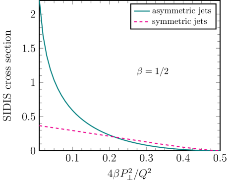
Figure 24: Contributions to the SIDIS cross section of 2+1 jet configurations with a soft quark ($\vartheta_{1}\ll 1$): the integrals appearing in Eqs. (141) (asymmetric $\bar{q}g$ dijet) and (D.1) (symmetric $\bar{q}g$ dijet) as functions of the combined variable $4\beta P_{\perp}^{2}/Q^{2}=x_{\rm min}-\beta$. The scattering amplitude is given by the MV model with a saturation scale $Q_{s}^{2}=0.88\,\mathrm{GeV}^{2}$ (in the fundamental representation).

Consider finally the case of a virtual photon with longitudinal polarisation. The respective contribution to diffractive (2+1)–jets with a soft quark, as shown in Eqs. (129)–(130), can be cast in the form of Eq. (217) with

$$h_{L}=\,4\vartheta_{2}\vartheta_{3}\frac{\tilde{Q}^{4}P^{2}_{\perp}}{(P_{\perp}^{2}+\tilde{Q}^{2})^{3}}\,=\,4\left(\frac{\beta}{x}\right)^{3}\frac{P_{\perp}^{2}}{Q^{2}}\,,$$ (233)

where the second equality follows after also using the $\delta$–function (D.1). This implies

$$\int{\rm d}\vartheta_{2}{\rm d}\vartheta_{3}\,\delta_{\vartheta}\,\delta\left(x-\beta\frac{P_{\perp}^{2}+\tilde{Q}^{2}}{\tilde{Q}^{2}}\right)\frac{h_{L}}{\vartheta_{3}} =\,\frac{\beta^{2}}{x^{3}}\,\frac{4\beta}{x-\beta}\frac{P_{\perp}^{2}}{Q^{2}}\,\frac{1}{1-2\vartheta_{*}}\,,$$ (234)

which gives no LT contribution after integration over $x$. Indeed, the relevant integral reads

$$\int_{x_{\rm min}}^{1}\frac{{\rm d}x}{x-\beta}\,\frac{4\beta P_{\perp}^{2}}{Q^{2}}\,\frac{1}{\sqrt{1-\frac{4\beta}{x-\beta}\frac{P_{\perp}^{2}}{Q^{2}}}}\,=\int_{t_{\rm min}}^{1-\beta}\frac{{\rm d}t}{t}\frac{t_{\rm min}}{\sqrt{1-\frac{t_{\rm min}}{t}}}\,,$$ (235)

and is quite similar to that in Eq. (226), except that it involves an additional factor $t_{\rm min}\sim{P_{\perp}^{2}}/{Q^{2}}$. Since the result of (226) is of order one (up to logarithms), it is clear that the result of (235) is of $\mathcal{O}{\left({P_{\perp}^{2}}/{Q^{2}}\right)}$, so its contribution to the SIDIS cross-section is of higher-twist order. From the above manipulations, it should be clear that this suppression is ultimately due to the factor $\vartheta_{2}\vartheta_{3}$ introduced by the splitting of the longitudinal photon.

D.2 The case of a soft gluon

For (2+1)-jets with a soft gluon, the analog of Eq. (132) reads (recall Eq. (66))

$$\frac{{\rm d}\sigma^{\gamma_{T}^{*}A\rightarrow q\bar{q}(g)}}{{\rm d}^{2}\!\bm{P}\,{\rm d}\ln(1/\beta)} \,=\int{\rm d}\vartheta_{1}{\rm d}\vartheta_{2}\frac{{\rm d}\sigma^{\gamma_{T}^{*}A\rightarrow q\bar{q}(g)XA}}{{\rm d}\vartheta_{1}{\rm d}\vartheta_{2}{\rm d}^{2}\!\bm{P}\,{\rm d}\ln(1/\beta)}$$ (236)

$$\,=\int{\rm d}\vartheta_{2}\int_{\beta}^{1}{\rm d}x\,\delta\left(x-\beta\,\frac{\bar{Q}^{2}+P_{\perp}^{2}}{\bar{Q}^{2}}\right)\tilde{H}_{T}(1-\vartheta_{2},\vartheta_{2},{Q}^{2},P_{\perp}^{2})\,xG_{\mathbb{P}}\left(x,x_{\mathbb{P}},{(1-x)P_{\perp}^{2}}\right).$$

where the hard momentum $\bm{P}$ is now the relative momentum of the quark-antiquark pair, whereas the semi-hard momentum $\bm{K}$ refers to the gluon. Also, $\bar{Q}^{2}=\vartheta_{1}\vartheta_{2}Q^{2}$, with $\vartheta_{1}+\vartheta_{2}=1$. The hard factor corresponding to a virtual photon with transverse polarisation has been shown in Eq. (60), whereas the gluon diffractive TMD (or the UGD of the Pomeron) is exhibited in Eqs. (62)–(63).

This $\delta$–function is treated similarly to Eq. (D.1), namely

$$\delta\left(x-\beta\,\frac{P_{\perp}^{2}+\bar{Q}^{2}}{\bar{Q}^{2}}\right) \,=\,\frac{\vartheta_{1}\vartheta_{2}}{x-\beta}\,\delta\left(\vartheta_{1}\vartheta_{2}-\frac{\beta}{x-\beta}\,\frac{P_{\perp}^{2}}{Q^{2}}\right)$$

$$\,=\,\frac{\beta}{(x-\beta)^{2}}\,\frac{P_{\perp}^{2}}{Q^{2}}\,\frac{\delta\left(\vartheta_{2}-\vartheta_{*}\right)+\delta\left(\vartheta_{2}-1+\vartheta_{*}\right)}{1-2\vartheta_{*}},$$ (237)

with $\vartheta_{*}$ as shown Eq. (220). This implies

$$\frac{P_{\perp}^{4}+\bar{Q}^{4}}{(P_{\perp}^{2}+\bar{Q}^{2})^{4}}\,=\,\frac{1}{P_{\perp}^{4}}\left(\frac{x-\beta}{x}\right)^{2}\left[\left(1-\frac{\beta}{x}\right)^{2}+\left(\frac{\beta}{x}\right)^{2}\right]=\,\frac{2}{P_{\perp}^{4}}\left(\frac{x-\beta}{x}\right)^{2}P_{qg}\left(\frac{\beta}{x}\right).$$ (238)

After integrating over $\vartheta_{2}$, one finds (notice that both solutions for $\vartheta_{2}$ give identical results)

$$\frac{{\rm d}\sigma_{{\rm soft}\,g}^{\gamma_{\scriptscriptstyle T}^{*}A\rightarrow q\bar{q}gA}}{{\rm d}^{2}\bm{P}\,{\rm d}\ln(1/\beta)}=\frac{4\pi^{2}\alpha_{\rm em}}{Q^{2}}\left(\sum e_{f}^{2}\right)\frac{\alpha_{s}}{\pi^{2}}\frac{1}{P_{\perp}^{2}}\int_{x_{\rm min}}^{1}\frac{{\rm d}x}{x}\frac{\beta}{x}\,P_{qg}\left(\frac{\beta}{x}\right)\frac{1-\frac{2\beta}{x-\beta}\frac{P_{\perp}^{2}}{Q^{2}}}{\sqrt{1-\frac{4\beta}{x-\beta}\frac{P_{\perp}^{2}}{Q^{2}}}}\,xG_{\mathbb{P}}\left(x,x_{\mathbb{P}},{(1-x)P_{\perp}^{2}}\right).$$ (239)

This differs from Eq. (142) in the main text via the lower limit, which is $x_{\rm min}>\beta$ (cf. Eq. (220)), and also via an additional factor inside the integrand, which for finite $x-\beta$ is formally of higher-twist order, but which could bring in complications from the limit $x\to\beta$, as we have seen in the case of a soft quark. Yet, in the present case, there are no such complications: the $g\to q\bar{q}$ splitting function $P_{qg}(\beta/x)$ is not singular in that limit, hence the leading twist contribution to Eq. (239) is correctly given by Eq. (142). In fact, the structure of the above integral is very similar to that previously encountered in the case of a soft quark, in relation with the interference contribution, cf. Eq. (228).

By the same argument, in this case there is no additional LT contribution from symmetric jets. This can also be understood from a diagrammatic viewpoint: the gluon decay must occur inside the target wavefunction in order to produce the $q\bar{q}$ pair which absorbs the virtual photon. So, in this case, there is no place for final state radiation within the context of collinear factorisation (and to the order of interest).

References

• (1) E. Iancu, A. Leonidov and L. McLerran, The Color glass condensate: An Introduction, hep-ph/0202270.
• (2) E. Iancu and R. Venugopalan, The color glass condensate and high energy scattering in QCD, hep-ph/0303204.
• (3) F. Gelis, E. Iancu, J. Jalilian-Marian and R. Venugopalan, The Color Glass Condensate, Ann.Rev.Nucl.Part.Sci. 60 (2010) 463 [1002.0333].
• (4) Y.V. Kovchegov and E. Levin, Quantum chromodynamics at high energy, Cambridge University Press (2012).
• (5) G.F. Sterman, An Introduction to quantum field theory, Cambridge University Press (8, 1993).
• (6) J. Collins, Foundations of Perturbative QCD, vol. 32 of Cambridge Monographs on Particle Physics, Nuclear Physics and Cosmology, Cambridge University Press (7, 2023), 10.1017/9781009401845.
• (7) F. Dominguez, C. Marquet, B.-W. Xiao and F. Yuan, Universality of Unintegrated Gluon Distributions at small x, Phys. Rev. D83 (2011) 105005 [1101.0715].
• (8) A. Metz and J. Zhou, Distribution of linearly polarized gluons inside a large nucleus, Phys. Rev. D 84 (2011) 051503 [1105.1991].
• (9) F. Dominguez, J.-W. Qiu, B.-W. Xiao and F. Yuan, On the linearly polarized gluon distributions in the color dipole model, Phys. Rev. D 85 (2012) 045003 [1109.6293].
• (10) E. Iancu and J. Laidet, Gluon splitting in a shockwave, Nucl.Phys. A916 (2013) 48 [1305.5926].
• (11) A. Dumitru, T. Lappi and V. Skokov, Distribution of Linearly Polarized Gluons and Elliptic Azimuthal Anisotropy in Deep Inelastic Scattering Dijet Production at High Energy, Phys. Rev. Lett. 115 (2015) 252301 [1508.04438].
• (12) P. Kotko, K. Kutak, C. Marquet, E. Petreska, S. Sapeta and A. van Hameren, Improved TMD factorization for forward dijet production in dilute-dense hadronic collisions, JHEP 09 (2015) 106 [1503.03421].
• (13) C. Marquet, E. Petreska and C. Roiesnel, Transverse-momentum-dependent gluon distributions from JIMWLK evolution, JHEP 10 (2016) 065 [1608.02577].
• (14) A. van Hameren, P. Kotko, K. Kutak, C. Marquet, E. Petreska and S. Sapeta, Forward di-jet production in p+Pb collisions in the small-x improved TMD factorization framework, JHEP 12 (2016) 034 [1607.03121].
• (15) C. Marquet, C. Roiesnel and P. Taels, Linearly polarized small-$x$ gluons in forward heavy-quark pair production, Phys. Rev. D 97 (2018) 014004 [1710.05698].
• (16) J.L. Albacete, G. Giacalone, C. Marquet and M. Matas, Forward dihadron back-to-back correlations in $pA$ collisions, Phys. Rev. D 99 (2019) 014002 [1805.05711].
• (17) A. Dumitru, V. Skokov and T. Ullrich, Measuring the Weizsäcker-Williams distribution of linearly polarized gluons at an electron-ion collider through dijet azimuthal asymmetries, Phys. Rev. C 99 (2019) 015204 [1809.02615].
• (18) R. Boussarie, H. Mäntysaari, F. Salazar and B. Schenke, The importance of kinematic twists and genuine saturation effects in dijet production at the Electron-Ion Collider, JHEP 09 (2021) 178 [2106.11301].
• (19) P. Kotko, K. Kutak, S. Sapeta, A.M. Stasto and M. Strikman, Estimating nonlinear effects in forward dijet production in ultra-peripheral heavy ion collisions at the LHC, Eur. Phys. J. C 77 (2017) 353 [1702.03063].
• (20) E. Iancu and Y. Mulian, Forward dijets in proton-nucleus collisions at next-to-leading order: the real corrections, JHEP 03 (2021) 005 [2009.11930].
• (21) P. Caucal, F. Salazar and R. Venugopalan, Dijet impact factor in DIS at next-to-leading order in the Color Glass Condensate, JHEP 11 (2021) 222 [2108.06347].
• (22) P. Taels, T. Altinoluk, G. Beuf and C. Marquet, Dijet photoproduction at low x at next-to-leading order and its back-to-back limit, JHEP 10 (2022) 184 [2204.11650].
• (23) F. Bergabo and J. Jalilian-Marian, One-loop corrections to dihadron production in DIS at small x, Phys. Rev. D 106 (2022) 054035 [2207.03606].
• (24) E. Iancu and Y. Mulian, Dihadron production in DIS at NLO: the real corrections, JHEP 07 (2023) 121 [2211.04837].
• (25) P. Caucal, F. Salazar, B. Schenke, T. Stebel and R. Venugopalan, Back-to-back inclusive dijets in DIS at small x: gluon Weizsäcker-Williams distribution at NLO, JHEP 08 (2023) 062 [2304.03304].
• (26) P. Caucal, F. Salazar, B. Schenke, T. Stebel and R. Venugopalan, Back-to-back inclusive dijets in DIS at small $x$: Complete NLO results and predictions, 2308.00022.
• (27) C. Marquet, Forward inclusive dijet production and azimuthal correlations in pA collisions, Nucl. Phys. A796 (2007) 41 [0708.0231].
• (28) J.L. Albacete and C. Marquet, Azimuthal correlations of forward di-hadrons in d+Au collisions at RHIC in the Color Glass Condensate, Phys. Rev. Lett. 105 (2010) 162301 [1005.4065].
• (29) A. Stasto, B.-W. Xiao and F. Yuan, Back-to-Back Correlations of Di-hadrons in dAu Collisions at RHIC, Phys.Lett. B716 (2012) 430 [1109.1817].
• (30) T. Lappi and H. Mäntysaari, Forward dihadron correlations in deuteron-gold collisions with the Gaussian approximation of JIMWLK, Nucl.Phys. A908 (2013) 51 [1209.2853].
• (31) L. Zheng, E. Aschenauer, J. Lee and B.-W. Xiao, Probing Gluon Saturation through Dihadron Correlations at an Electron-Ion Collider, Phys. Rev. D 89 (2014) 074037 [1403.2413].
• (32) A. Mueller, B.-W. Xiao and F. Yuan, Sudakov double logarithms resummation in hard processes in the small-x saturation formalism, Phys. Rev. D 88 (2013) 114010 [1308.2993].
• (33) M. Wusthoff, Large rapidity gap events in deep inelastic scattering, Phys. Rev. D 56 (1997) 4311 [hep-ph/9702201].
• (34) K.J. Golec-Biernat and M. Wusthoff, Saturation in diffractive deep inelastic scattering, Phys. Rev. D60 (1999) 114023 [hep-ph/9903358].
• (35) A. Hebecker, Diffractive parton distributions in the semiclassical approach, Nucl. Phys. B 505 (1997) 349 [hep-ph/9702373].
• (36) W. Buchmuller, T. Gehrmann and A. Hebecker, Inclusive and diffractive structure functions at small x, Nucl. Phys. B 537 (1999) 477 [hep-ph/9808454].
• (37) F. Hautmann, Z. Kunszt and D.E. Soper, Diffractive deeply inelastic scattering of hadronic states with small transverse size, Phys. Rev. Lett. 81 (1998) 3333 [hep-ph/9806298].
• (38) F. Hautmann, Z. Kunszt and D.E. Soper, Hard scattering factorization and light cone Hamiltonian approach to diffractive processes, Nucl. Phys. B 563 (1999) 153 [hep-ph/9906284].
• (39) F. Hautmann and D.E. Soper, Color transparency in deeply inelastic diffraction, Phys. Rev. D 63 (2001) 011501 [hep-ph/0008224].
• (40) K.J. Golec-Biernat and M. Wusthoff, Diffractive parton distributions from the saturation model, Eur. Phys. J. C 20 (2001) 313 [hep-ph/0102093].
• (41) I. Balitsky and G.A. Chirilli, Photon impact factor in the next-to-leading order, Phys. Rev. D83 (2011) 031502 [1009.4729].
• (42) I. Balitsky and G.A. Chirilli, Photon impact factor and $k_{T}$-factorization for DIS in the next-to-leading order, Phys. Rev. D87 (2013) 014013 [1207.3844].
• (43) G. Beuf, Dipole factorization for DIS at NLO: Loop correction to the $\gamma^{*}_{T,L}\to q\overline{q}$ light-front wave functions, Phys. Rev. D 94 (2016) 054016 [1606.00777].
• (44) G. Beuf, Dipole factorization for DIS at NLO: Combining the $q\bar{q}$ and $q\bar{q}g$ contributions, Phys. Rev. D96 (2017) 074033 [1708.06557].
• (45) G. Beuf, T. Lappi and R. Paatelainen, Massive quarks in NLO dipole factorization for DIS: Longitudinal photon, Phys. Rev. D 104 (2021) 056032 [2103.14549].
• (46) G. Beuf, T. Lappi and R. Paatelainen, Massive Quarks at One Loop in the Dipole Picture of Deep Inelastic Scattering, Phys. Rev. Lett. 129 (2022) 072001 [2112.03158].
• (47) G. Beuf, T. Lappi and R. Paatelainen, Massive quarks in NLO dipole factorization for DIS: Transverse photon, Phys. Rev. D 106 (2022) 034013 [2204.02486].
• (48) G. Beuf, H. Hänninen, T. Lappi, Y. Mulian and H. Mäntysaari, Diffractive deep inelastic scattering at NLO in the dipole picture: The $q\bar{q}g$ contribution, Phys. Rev. D 106 (2022) 094014 [2206.13161].
• (49) G. Beuf, T. Lappi, H. Mäntysaari, R. Paatelainen and J. Penttala, Diffractive deep inelastic scattering at NLO in the dipole picture, 2401.17251.
• (50) E. Iancu, A.H. Mueller, D.N. Triantafyllopoulos and S.Y. Wei, Saturation effects in SIDIS at very forward rapidities, JHEP 07 (2021) 196 [2012.08562].
• (51) Y. Hatta, B.-W. Xiao and F. Yuan, Semi-inclusive diffractive deep inelastic scattering at small x, Phys. Rev. D 106 (2022) 094015 [2205.08060].
• (52) E. Iancu, A.H. Mueller and D.N. Triantafyllopoulos, Probing Parton Saturation and the Gluon Dipole via Diffractive Jet Production at the Electron-Ion Collider, Phys. Rev. Lett. 128 (2022) 202001 [2112.06353].
• (53) E. Iancu, A.H. Mueller, D.N. Triantafyllopoulos and S.Y. Wei, Gluon dipole factorisation for diffractive dijets, JHEP 10 (2022) 103 [2207.06268].
• (54) L. Trentadue and G. Veneziano, Fracture functions: An Improved description of inclusive hard processes in QCD, Phys. Lett. B 323 (1994) 201.
• (55) A. Berera and D.E. Soper, Behavior of diffractive parton distribution functions, Phys. Rev. D 53 (1996) 6162 [hep-ph/9509239].
• (56) J.C. Collins, Proof of factorization for diffractive hard scattering, Phys. Rev. D 57 (1998) 3051 [hep-ph/9709499].
• (57) F. Salazar and B. Schenke, Diffractive dijet production in impact parameter dependent saturation models, Phys. Rev. D 100 (2019) 034007 [1905.03763].
• (58) R. Boussarie, A. Grabovsky, L. Szymanowski and S. Wallon, Impact factor for high-energy two and three jets diffractive production, JHEP 09 (2014) 026 [1405.7676].
• (59) R. Boussarie, A. Grabovsky, L. Szymanowski and S. Wallon, On the one loop ${\gamma}^{\left(\ast\right)}\to q\overline{q}$ impact factor and the exclusive diffractive cross sections for the production of two or three jets, JHEP 11 (2016) 149 [1606.00419].
• (60) M. Fucilla, A.V. Grabovsky, E. Li, L. Szymanowski and S. Wallon, NLO computation of diffractive di-hadron production in a saturation framework, JHEP 03 (2023) 159 [2211.05774].
• (61) F. Hautmann, Diffractive jet production in lepton hadron collisions, JHEP 10 (2002) 025 [hep-ph/0209320].
• (62) D. Britzger, J. Currie, T. Gehrmann, A. Huss, J. Niehues and R. Žlebčík, Dijet production in diffractive deep-inelastic scattering in next-to-next-to-leading order QCD, Eur. Phys. J. C 78 (2018) 538 [1804.05663].
• (63) H1 collaboration, Tests of QCD factorisation in the diffractive production of dijets in deep-inelastic scattering and photoproduction at HERA, Eur. Phys. J. C 51 (2007) 549 [hep-ex/0703022].
• (64) V. Guzey and M. Klasen, Diffractive dijet photoproduction in ultraperipheral collisions at the LHC in next-to-leading order QCD, JHEP 04 (2016) 158 [1603.06055].
• (65) M. Fucilla, A. Grabovsky, E. Li, L. Szymanowski and S. Wallon, Diffractive single hadron production in a saturation framework at the NLO, 2310.11066.
• (66) V. Gribov and L. Lipatov, Deep inelastic e p scattering in perturbation theory, Sov.J.Nucl.Phys. 15 (1972) 438.
• (67) G. Altarelli and G. Parisi, Asymptotic Freedom in Parton Language, Nucl.Phys. B126 (1977) 298.
• (68) Y.L. Dokshitzer, Calculation of the Structure Functions for Deep Inelastic Scattering and e+ e- Annihilation by Perturbation Theory in Quantum Chromodynamics., Sov.Phys.JETP 46 (1977) 641.
• (69) E. Iancu, A.H. Mueller, D.N. Triantafyllopoulos and S.Y. Wei, Probing gluon saturation via diffractive jets in ultra-peripheral nucleus-nucleus collisions, Eur. Phys. J. C 83 (2023) 1078 [2304.12401].
• (70) A. Accardi et al., Electron Ion Collider: The Next QCD Frontier: Understanding the glue that binds us all, Eur. Phys. J. A 52 (2016) 268 [1212.1701].
• (71) E. Aschenauer, S. Fazio, J. Lee, H. Mantysaari, B. Page, B. Schenke et al., The electron–ion collider: assessing the energy dependence of key measurements, Rept. Prog. Phys. 82 (2019) 024301 [1708.01527].
• (72) R. Abdul Khalek et al., Snowmass 2021 White Paper: Electron Ion Collider for High Energy Physics, in 2022 Snowmass Summer Study, 3, 2022 [2203.13199].
• (73) ATLAS collaboration, U. Heinz, O. Evdokimov and P. Jacobs, eds., Photo-nuclear dijet production in ultra-peripheral Pb+Pb collisions, ATLAS-CONF-2017-011 (2017) .
• (74) ATLAS collaboration, Photo-nuclear jet production in ultra-peripheral Pb+Pb collisions at $\sqrt{s}_{\text{NN}}=5.02$ TeV with the ATLAS detector, ATLAS-CONF-2022-021 (2022) .
• (75) CMS collaboration, Angular correlations in exclusive dijet photoproduction in ultra-peripheral PbPb collisions at $\sqrt{s_{NN}}=5.02~{}\mathrm{TeV}$, CMS-PAS-HIN-18-011 (2020) .
• (76) CMS collaboration, Azimuthal Correlations within Exclusive Dijets with Large Momentum Transfer in Photon-Lead Collisions, Phys. Rev. Lett. 131 (2023) 051901 [2205.00045].
• (77) I. Balitsky, Operator expansion for high-energy scattering, Nucl. Phys. B463 (1996) 99 [hep-ph/9509348].
• (78) Y.V. Kovchegov, Small-x F2 structure function of a nucleus including multiple pomeron exchanges, Phys. Rev. D60 (1999) 034008 [hep-ph/9901281].
• (79) E. Iancu, J. Madrigal, A. Mueller, G. Soyez and D. Triantafyllopoulos, Resumming double logarithms in the QCD evolution of color dipoles, Phys.Lett. B744 (2015) 293 [1502.05642].
• (80) B. Ducloué, E. Iancu, A.H. Mueller, G. Soyez and D.N. Triantafyllopoulos, Non-linear evolution in QCD at high-energy beyond leading order, JHEP 04 (2019) 081 [1902.06637].
• (81) E. Iancu and Y. Mulian, Forward trijet production in proton–nucleus collisions, Nucl. Phys. A 985 (2019) 66 [1809.05526].
• (82) J. Jalilian-Marian, A. Kovner, A. Leonidov and H. Weigert, The BFKL equation from the Wilson renormalization group, Nucl. Phys. B504 (1997) 415 [hep-ph/9701284].
• (83) J. Jalilian-Marian, A. Kovner, A. Leonidov and H. Weigert, The Wilson renormalization group for low x physics: Towards the high density regime, Phys.Rev. D59 (1998) 014014 [hep-ph/9706377].
• (84) A. Kovner, J.G. Milhano and H. Weigert, Relating different approaches to nonlinear QCD evolution at finite gluon density, Phys. Rev. D62 (2000) 114005 [hep-ph/0004014].
• (85) H. Weigert, Unitarity at small Bjorken x, Nucl. Phys. A703 (2002) 823 [hep-ph/0004044].
• (86) E. Iancu, A. Leonidov and L.D. McLerran, Nonlinear gluon evolution in the color glass condensate. I, Nucl. Phys. A692 (2001) 583 [hep-ph/0011241].
• (87) E. Iancu, A. Leonidov and L.D. McLerran, The renormalization group equation for the color glass condensate, Phys. Lett. B510 (2001) 133 [hep-ph/0102009].
• (88) E. Ferreiro, E. Iancu, A. Leonidov and L. McLerran, Nonlinear gluon evolution in the color glass condensate. II, Nucl. Phys. A703 (2002) 489 [hep-ph/0109115].
• (89) C. Marquet and H. Weigert, New observables to test the Color Glass Condensate beyond the large- $N_{c}$ limit, Nucl. Phys. A 843 (2010) 68 [1003.0813].
• (90) H. Mäntysaari, N. Mueller, F. Salazar and B. Schenke, Multigluon Correlations and Evidence of Saturation from Dijet Measurements at an Electron-Ion Collider, Phys. Rev. Lett. 124 (2020) 112301 [1912.05586].
• (91) B. Rodriguez-Aguilar, D.N. Triantafyllopoulos and S.Y. Wei, Incoherent diffractive dijet production in electron DIS off nuclei at high energy, Phys. Rev. D 107 (2023) 114007 [2302.01106].
• (92) L.D. McLerran and R. Venugopalan, Computing quark and gluon distribution functions for very large nuclei, Phys. Rev. D49 (1994) 2233 [hep-ph/9309289].
• (93) L.D. McLerran and R. Venugopalan, Green’s functions in the color field of a large nucleus, Phys. Rev. D50 (1994) 2225 [hep-ph/9402335].
• (94) Y.V. Kovchegov and E. Levin, Diffractive dissociation including multiple pomeron exchanges in high parton density QCD, Nucl. Phys. B 577 (2000) 221 [hep-ph/9911523].
• (95) Y. Hatta, E. Iancu, C. Marquet, G. Soyez and D. Triantafyllopoulos, Diffusive scaling and the high-energy limit of deep inelastic scattering in QCD at large N(c), Nucl.Phys. A773 (2006) 95 [hep-ph/0601150].
• (96) G. Beuf, Improving the kinematics for low-x QCD evolution equations in coordinate space, Phys.Rev. D89 (2014) 074039 [1401.0313].
• (97) B. Ducloué, E. Iancu, G. Soyez and D. Triantafyllopoulos, HERA data and collinearly-improved BK dynamics, Phys. Lett. B 803 (2020) 135305 [1912.09196].
• (98) T. Altinoluk, N. Armesto, G. Beuf and A.H. Rezaeian, Diffractive Dijet Production in Deep Inelastic Scattering and Photon-Hadron Collisions in the Color Glass Condensate, Phys. Lett. B 758 (2016) 373 [1511.07452].
• (99) Y. Hatta, B.-W. Xiao and F. Yuan, Probing the Small- x Gluon Tomography in Correlated Hard Diffractive Dijet Production in Deep Inelastic Scattering, Phys. Rev. Lett. 116 (2016) 202301 [1601.01585].
• (100) Y. Hagiwara, Y. Hatta, R. Pasechnik, M. Tasevsky and O. Teryaev, Accessing the gluon Wigner distribution in ultraperipheral $pA$ collisions, Phys. Rev. D 96 (2017) 034009 [1706.01765].
• (101) H. Mäntysaari, N. Mueller and B. Schenke, Diffractive Dijet Production and Wigner Distributions from the Color Glass Condensate, Phys. Rev. D 99 (2019) 074004 [1902.05087].
• (102) Y. Hatta, B.-W. Xiao, F. Yuan and J. Zhou, Azimuthal angular asymmetry of soft gluon radiation in jet production, Phys. Rev. D 104 (2021) 054037 [2106.05307].
• (103) D.Y. Shao, Y. Shi, C. Zhang, J. Zhou and Y.-j. Zhou, Revisiting azimuthal angular asymmetries in diffractive di-jet production, 2402.05465.