Solitons of the mean curvature flow in $\mathbb{S}^{2}\times\mathbb{R}$

Abstract.

A soliton of the mean curvature flow in the product space $\mathbb{S}^{2}\times\mathbb{R}$ is a surface whose mean curvature $H$ satisfies the equation $H=\langle N,X\rangle$, where $N$ is the unit normal of the surface and $X$ is a Killing vector field. In this paper we consider the vector field tangent to the fibers and the vector field associated to rotations about an axis of $\mathbb{S}^{2}$, respectively. We give a classification of the solitons with respect to these vector fields assuming that the surface is invariant under a one-parameter group of vertical translations or rotations of $\mathbb{S}^{2}$.

1. Introduction

Let $\psi\colon\Sigma\to\mathbb{R}^{3}$ be an immersion of a surface $\Sigma$ in Euclidean space $\mathbb{R}^{3}$. A variation $\{\psi_{t}\colon\Sigma\to\mathbb{R}^{3}:t\in[0,T)\}$, $T>0$, $\psi_{0}=\psi$, evolves by the mean curvature flow (MCF in short) if $\displaystyle\frac{\partial\psi_{t}}{\partial t}=H(\psi_{t})N(\psi_{t})$, where $H(\psi_{t})$ is the mean curvature of $\psi_{t}$ and $N(\psi_{t})$ is its unit normal. The surface $\Sigma$ is called a soliton of MCF if the evolution of $\Sigma$ under a one-parameter family of dilations or isometries remains constant. An important type of solitons are the translators whose shape is invariant by translations along a direction $\vec{v}\in\mathbb{R}^{3}$. Translators are characterized by the equation $H=\langle N,\vec{v}\rangle$, where $H$ and $N$ are the mean curvature and unit normal of $\Sigma$ respectively. Translators play a special role in the theory of MCF because they are, after rescaling, a type of singularities of the MCF according to Huisken and Sinestrari [6]. In the meantime, the development of the theory of solitons of the MCF in other ambient space has been developed. Without to be complete, we refer: a general product space $M^{2}\times\mathbb{R}$ [9]; hyperbolic space [3, 4, 8, 11]; the product $\mathbb{H}^{2}\times\mathbb{R}$ [1, 2, 5, 7]; the Sol space [14]; the Heisenberg group [15]; the special linear group [10].

In this paper, we focus on solitons in the product space $\mathbb{S}^{2}\times\mathbb{R}$, where $\mathbb{S}^{2}$ is the unit sphere of $\mathbb{R}^{3}$. Looking in the equation $H=\langle N,\vec{v}\rangle$, it is natural to replace $\vec{v}$ by a Killing vector of the space, which motivates the following definition.

Definition 1.1.

Let $X\in\mathfrak{X}(\mathbb{S}^{2}\times\mathbb{R})$ be a Killing vector field. A surface $\Sigma$ in $\mathbb{S}^{2}\times\mathbb{R}$ is said to be a $X$-soliton if its mean curvature $H$ and unit normal vector $N$ satisfy

$$H=\langle N,X\rangle.$$ (1)

In this paper, $H$ is the sum of the principal curvatures of the surface. The dimension of Killing vector fields in the space $\mathbb{S}^{2}\times\mathbb{R}$ is $4$. Taking coordinates $(x,y,z,t)$ in $\mathbb{S}^{2}\times\mathbb{R}$, a relevant Killing vector field is $V=\partial_{t}$. Here $V$ is tangent to the fibers of the natural submersion $\mathbb{S}^{2}\times\mathbb{R}\to\mathbb{S}^{2}$. Other Killing vector fields come from the rotations of $\mathbb{S}^{2}$. After renaming coordinates, consider the vector field $R=-y\partial_{x}+x\partial_{y}$ about the $z$-axis of $\mathbb{S}^{2}$. Examples of solitons are the following.

1. Cylinders over geodesic of $\mathbb{S}^{2}$ are $V$-solitons. Indeed, let $\Sigma=C\times\mathbb{R}$ be a surface constructed as a cylinder over a curve $C$ of $\mathbb{S}^{2}$. Then the mean curvature of $\Sigma$ is $H=\kappa$, where $\kappa$ the curvature of $C$. Since the unit normal vector $N$ of $\Sigma$ is orthogonal to $\partial_{t}$, then $\langle N,V\rangle=0$. Thus $\Sigma$ is a $V$-soliton if and only if $\kappa=0$. Thus $C$ is a geodesic of $\mathbb{S}^{2}$.

2. Slices $\mathbb{S}^{2}\times\{t_{0}\}$, $t_{0}\in\mathbb{R}$, are $R$-solitons. Notice that $H=0$ because a slice is totally geodesic. Since $N=\partial_{t}$, then $\langle N,R\rangle=0$, proving that $H=\langle N,R\rangle$.

In this paper, we are interested in examples of $V$-solitons and $R$-solitons that are invariant by a one-parameter group of isometries of $\mathbb{S}^{2}\times\mathbb{R}$. Here we consider two types of such surfaces. First, vertical surfaces which are invariant by vertical translations in the $t$-coordinate. Second, rotational surfaces, which are invariant by a group of rotations about an axis of $\mathbb{S}^{2}$. Under these geometric conditions on the surfaces, we give a full classifications of $V$-solitons (Sect. 3) and $R$-solitons (Sect. 4).

2. Preliminaries

In this section, we compute each one of the terms of Eq. (1) for vertical and rotational surfaces. The isometry group of $\mathbb{S}^{2}\times\mathbb{R}$ isomorphic to $\mbox{Isom}(\mathbb{S}^{2})\times\mbox{Isom}(\mathbb{R})$. The group $\mbox{Isom}(\mathbb{S}^{2})$ is generated by the identity, the antipodal map, rotations and reflections. The group $\mbox{Isom}(\mathbb{R})$ contains the identity, translations, and reflections. Therefore there are two important one-parameter groups of isometries in $\mathbb{S}^{2}\times\mathbb{R}$: vertical translations in the factor $\mathbb{R}$ and rotations in the factor $\mathbb{S}^{2}$. This leads two types of invariant surfaces.

1. Vertical surfaces. A vertical translation is a map of type $T_{\lambda}\colon\mathbb{S}^{2}\times\mathbb{R}\to\mathbb{S}^{2}\times\mathbb{R}$ defined by $T_{\lambda}(p,t)=(p,t+\lambda)$, where $\lambda$ is fixed. This defines a one-parameter group of vertical translations $\mathcal{T}=\{T_{\lambda}:\lambda\in\mathbb{R}\}$. A vertical surface is a surface $\Sigma$ invariant by the group $\mathcal{T}$, that is, $T_{\lambda}(\Sigma)\subset\Sigma$ for all $\lambda\in\mathbb{R}$. The generating curve of $\Sigma$ is a curve $\alpha\colon I\subset\mathbb{R}\to\mathbb{S}^{2}$ in the unit sphere $\mathbb{S}^{2}$. Let us write this curve as

   $$\alpha(s)=(\cos u(s)\cos v(s),\cos u(s)\sin v(s),\sin u(s)),$$ (2)

   for some smooth functions $u=u(s)$ and $v=v(s)$. Then a parametrization of $\Sigma$ is

   $$\Psi(s,t)=(\cos u(s)\cos v(s),\cos u(s)\sin v(s),\sin u(s),t),\quad s\in I,t\in\mathbb{R}.$$ (3)

   In what follows, we parametrize the curve $\beta(s)=(u(s),v(s))$ to have

   $$u^{\prime}(s)=\cos u(s)\cos\theta(s),\quad v^{\prime}(s)=\sin\theta(s).$$

2. Rotational surfaces. These surfaces are invariant by rotations of $\mathbb{S}^{2}$. To be precise, and after a choice of coordinates on $\mathbb{S}^{2}$, a rotation in $\mathbb{S}^{2}\times\mathbb{R}$ about the $z$-axis is a map $\mathcal{R}_{\varphi}\colon\mathbb{S}^{2}\times\mathbb{R}\to\mathbb{S}^{2}\times\mathbb{R}$, given by

   $$R_{\varphi}=\left(\begin{array}[]{llll}\cos\varphi&-\sin\varphi&0&0\\ \sin\varphi&\cos\varphi&0&0\\ 0&0&1&0\\ 0&0&0&1\end{array}\right).$$

   The set $\mathcal{R}=\{\mathcal{R}_{\varphi}:\varphi\in\mathbb{R}\}$ of all $\mathcal{R}_{\varphi}$, is a one-parameter group of rotations, that is ${\mathrm{SO}}(2)$. A rotational surface is a surface $\Sigma$ invariant by the group $\mathcal{R}$, that is, $\mathcal{R}_{\varphi}(\Sigma)\subset\Sigma$ for all $\varphi\in\mathbb{R}$. The generating curve of $\Sigma$ is a curve $\alpha$ contained in the $xzt$-hyperplane which we suppose parametrized by

   $$\alpha(s)=(\cos u(s),0,\sin u(s),v(s)),\quad s\in I\subset\mathbb{R},$$ (4)

   where $u=u(s)$ and $v=v8s)$ are smooth functions. Then a parametrization of $\Sigma$ is

   $$\Psi(s,\varphi)=(\cos u(s)\cos\varphi,\cos u(s)\sin\varphi,\sin u(s),v(s)),\quad s\in I,\varphi\in\mathbb{R}.$$ (5)

   From now, suppose that the the curve $\beta(s)=(u(s),v(s))$ obtained from $\alpha$ in (4) is parametrized by the Euclidean arc-length, that is,

   $$u^{\prime}(s)=\cos\theta(s),\quad v^{\prime}(s)=\sin\theta(s),$$

   for some smooth function $\theta=\theta(s)$. Notice that $\theta^{\prime}$ is the curvature of $\beta$ as planar curve of $\mathbb{R}^{2}$.

We now compute the mean curvature $H$ and the unit normal vector $N$ of vertical surfaces and rotational surfaces.

Proposition 2.1.

Suppose that $\Sigma$ is a vertical surface parametrized by (3). Then the unit normal vector $N$ is

$$N=(\cos\theta\sin v-\sin\theta\sin u\cos v,-\cos\theta\cos v-\sin\theta\sin u\sin v,\sin\theta\cos u,0),$$ (6)

and the mean curvature $H$ is

$$H=\tan u\sin\theta-\frac{\theta^{\prime}}{\cos u}.$$ (7)

Proof.

Suppose that $\Sigma$ is parametrized by (3). Then the tangent plane each point of $\Sigma$ is spanned by $\{\Psi_{s},\Psi_{t}\}$, where

$$\begin{split}\Psi_{s}&=(-\cos u(\cos\theta\sin u\cos v+\sin\theta\sin v),\cos u(\sin\theta\cos v-\cos\theta\sin u\sin v),\cos\theta\cos^{2}u,0),\\ \Psi_{t}&=(0,0,0,1).\end{split}$$ (8)

A straightforward computation yields that the unit normal vector is (6).

As usually, denote by $g_{ij}$ the coefficients of the first fundamental form of $\Psi$, where

$$g_{11}=\langle\Psi_{s},\Psi_{s}\rangle,\quad g_{12}=\langle\Psi_{s},\Psi_{t}\rangle,\quad g_{22}=\langle\Psi_{t},\Psi_{t}\rangle.$$

The formula of $H$ is

$$H=\frac{g_{22}b_{11}-2g_{12}b_{12}+g_{11}b_{22}}{g_{11}g_{22}-{g_{12}}^{2}},$$

where $b_{ij}$ are the coefficients of the second fundamental form. Here

$$b_{11}=-\langle N_{s},\Psi_{s}\rangle,\quad b_{12}=-\langle N_{s},\Psi_{t}\rangle,\quad b_{22}=-\langle N_{t},\Psi_{t}\rangle.$$

A computation of $g_{ij}$ gives $g_{11}=g_{22}=(\cos u)^{2}$ and $g_{12}=0$. In particular, $\cos u(s)\not=0$ for all $s\in I$. Then $g_{11}g_{22}-g_{12}^{2}=(\cos u)^{4}$. For the coefficients of the second fundamental, we have $b_{12}=b_{22}=0$ and

$$b_{11}=\cos u(\sin\theta\sin-\theta^{\prime}).$$ (9)

Then the mean curvature $H$ is (7). ∎

Proposition 2.2.

Suppose that $\Sigma$ is a rotational surface parametrized by (5). Then the unit normal vector $N$ is

$$N(s,\varphi)=(\sin\theta\sin u\cos\varphi,\sin\theta\sin u\sin\varphi,-\sin\theta\cos u,\cos\theta),$$ (10)

and the mean curvature $H$ is

$$H=\theta^{\prime}-\sin\theta\tan u.$$ (11)

Proof.

From (3), the basis $\{\Psi_{s},\Psi_{t}\}$ at each tangent plane of $\Sigma$ is

$$\begin{split}\Psi_{s}(s,\varphi)&=(-u^{\prime}\sin u\cos\varphi,-u^{\prime}\sin u\sin\varphi,u^{\prime}\cos u,v^{\prime}),\\ \Psi_{\varphi}(s,\varphi)&=(-\sin\varphi\cos u,\cos\varphi\cos u,0,0).\end{split}$$ (12)

Thus $g_{11}=1$, $g_{12}=0$ and $g_{22}=\cos^{2}u$, in particular, $\cos u\not=0$. As a consequence, the unit normal vector $N$ is (10). The computation of the coefficients of the second fundamental form gives

$$\begin{split}b_{11}&=\theta^{\prime}\\ b_{12}&=0\\ b_{22}&=-\sin\theta\sin u\cos u.\end{split}$$ (13)

Hence we deduce that the expression of $H$ is (11).

∎

3. The class of $V$-solitons

Let the vector field

$$V=\partial_{t}.$$ (14)

The fact that $V$ is tangent to the fibers of the submersion $\mathbb{S}^{2}\times\mathbb{R}\to\mathbb{S}^{2}$ makes that $V$ has special properties. For example, $V$-solitons of $\mathbb{S}^{2}\times\mathbb{R}$ can be viewed as weighted minimal surfaces in a space with density. So, let $e^{t}dA$ and $e^{t}dV$ the area and volume of $\mathbb{S}^{2}\times\mathbb{R}$ with a weight $e^{t}$, where $t$ is the last coordinate of the space. Considering the energy functional $\Omega\mapsto E(\Omega)=\int_{\Omega}e^{t}dA$ defined for compact subdomains $\Omega\subset\Sigma$, a critical point of this functional, also called a weighted minimal surface, is a surface characterized by the equation $H-\langle N,\nabla t\rangle=0$, where $\nabla$ is the gradient in $\mathbb{S}^{2}\times\mathbb{R}$. Since $\nabla t=\partial_{t}=V$, we have proved that a weighted minimal surface in $(\mathbb{S}^{2}\times\mathbb{R},e^{t}\langle,\rangle)$ is a $V$-soliton. A property of weighted minimal surfaces is they satisfy a principle of tangency as a consequence of the Hopf maximum principle for elliptic equations of divergence type. In our context, the tangency principle asserts that if two $V$-solitons $\Sigma_{1}$ and $\Sigma_{2}$ touch at some interior point $p\in\Sigma_{1}\cap\Sigma_{2}$ and one surface is in one side of the other around $p$, then $\Sigma_{1}$ and $\Sigma_{2}$ coincide in a neighborhood of $p$. The following result proves that slices are the only closed $V$-solitons.

Theorem 3.1.

Slices $\mathbb{S}^{2}\times\{t_{0}\}$, $t_{0}\in\mathbb{R}$, are the only closed (compact without boundary) $V$-solitons in $\mathbb{S}^{2}\times\mathbb{R}$.

Proof.

Let $\psi\colon\Sigma\to\mathbb{S}^{2}\times\mathbb{R}$ be a closed $V$-soliton. Define on $\Sigma$ the height function $h\colon\Sigma\to\mathbb{R}$ by $h(q)=\langle\psi(q),\partial_{t}\rangle$. It is known that for any surface of $\mathbb{S}^{2}\times\mathbb{R}$, the Laplacian of $h$ is $\Delta h=H\langle N,\partial_{t}\rangle$ [16].

Using that $\Sigma$ is a $V$-soliton, then $\Delta h=\langle N,\partial_{t}\rangle^{2}=\langle N,V\rangle^{2}$. Integrating in $\Sigma$, the divergence theorem yields $\int_{\Sigma}\langle N,V\rangle^{2}=0$. Thus $\langle N,V\rangle=0$ on $\Sigma$ and $H=0$. In particular, $\Delta h=0$. By the maximum principle, $h$ is a constant function, namely $h(q)=t_{0}$, for some $t_{0}\in\mathbb{R}$. This proves that $\Sigma\subset\mathbb{S}^{2}\times\{t_{0}\}$ and thus, both surfaces coincide. ∎

We begin with the study of $V$-solitons invariant by the group $\mathcal{T}$. We prove that any vertical $V$-soliton is trivial in the sense that it is a minimal surface, even more, we prove that it is a cylinder of type $\mathbb{S}^{1}\times\mathbb{R}\subset\mathbb{S}^{2}\times\mathbb{R}$.

Theorem 3.2.

Suppose that $\Sigma$ is a vertical surface. Then $\Sigma$ is a $V$-soliton if and only its generating curve is a geodesic of $\mathbb{S}^{2}$ and $\Sigma$ is a vertical surface on a geodesic of $\mathbb{S}^{2}$.

Proof.

Let $\Sigma$ be a vertical surface. Since the vertical lines are fibers of the submersion $\mathbb{S}^{2}\times\mathbb{R}\to\mathbb{S}^{2}$, the mean curvature $H$ of $\Sigma$ is $H=\kappa$, where $\kappa$ is the curvature of $\alpha$. Moreover, the unit normal vector is horizontal, hence $\langle N,V\rangle=0$. This proves the result. ∎

We now study $V$-solitons of rotational type. As we have indicated in the previous section, we can assume that the rotation axis is the $z$-axis. Thus a rotational surface $\Sigma$ can be parametrized by (5).

An immediate example of rotational $V$-soliton is the cylinder $\mathcal{C}=(\mathbb{S}^{1}\times\{0\})\times\mathbb{R}$. This surface corresponds with the curve $(u(s),v(s))=(0,s)$, $s\in\mathbb{R}$, in (4). Thus $\alpha(s)=(1,0,0,s)$ is the vertical line through the point $(1,0,0)\in\mathbb{S}^{2}$. The unit normal $N$ is orthogonal to $V$. Since the generating curve is a geodesic of $\mathbb{S}^{2}$, the surface is minimal, proving that $\mathcal{C}$ is a $V$-soliton. This surface is also a vertical $R$-soliton (Thm. 3.2). We now characterize rotational $V$-solitons in terms of its generating curve $\alpha$.

Proposition 3.3.

Let $\Sigma$ be a rotational surface in $\mathbb{S}^{2}\times\mathbb{R}$. If $\Sigma$ is parametrized by (5), then $\Sigma$ is a $V$-soliton if and only if the generating curve $\alpha$ satisfies

$$\left\{\begin{split}u^{\prime}&=\cos\theta\\ v^{\prime}&=\sin\theta\\ \theta^{\prime}&=\sin\theta\tan u+\cos\theta\end{split}\right.$$ (15)

Proof.

This is an immediate consequence of Prop. 2.2. Indeed, from the expression of $N$ in (10), we have

$$\langle N,V\rangle=\cos\theta.$$

Using (11), then Eq. (1) is $\theta^{\prime}=\sin\theta\tan u+\cos\theta$.

∎

We now study the solutions of (15), describing their main geometric properties. Recall that $\cos u\not=0$ by regularity of the surface (Prop. 2.2). Since the last equation of (15) does not depend on $v$, we can study the solutions $\alpha$ of (15) projecting in the $(u,\theta)$-plane, which in turn leads to the planar autonomous ordinary system

$$\left\{\begin{split}u^{\prime}&=\cos\theta\\ \theta^{\prime}&=\sin\theta\tan u+\cos\theta.\end{split}\right.$$ (16)

The phase plane of (16) is depicted in Fig. 1. By regularity of the surface, $u(s)\in(-\pi/2,\pi/2)$. Thus the phase plane of (16) is the set

$$A=\{(u,\theta)\colon u\in(\frac{\pi}{2},\frac{\pi}{2}),\theta\in\mathbb{R}\}.$$

The trajectories of (16) are the solutions $\gamma(s)=(u(s),\theta(s))$ of (16) when regarded in $A$ and once initial conditions $(u_{0},\theta_{0})\in A$ have been fixed. These trajectories foliate $A$ as a consequence of the existence and uniqueness of the Cauchy problem of (16).

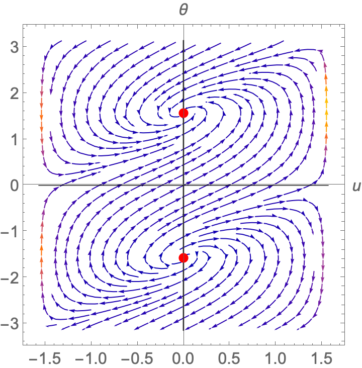
Figure 1. The $(u,\theta)$-phase plane of (16). The red points are the equilibrium points $(0,\pm\frac{\pi}{2})$, where the surface is the cylinder $\mathcal{C}$.

The equilibrium points of (16) are $(u,\theta)=(0,\frac{\pi}{2})$ and $(u,\theta)=(0,-\frac{\pi}{2})$. The rest of equilibrium points can be obtained by translations by multiples of $\pi$ in the $\theta$-coordinate. If $(u,\theta)=(0,\frac{\pi}{2})$, then $u(s)=0$, $v(s)=s$. Thus the generating curve $\alpha$ is the vertical fiber at $(1,0,0)\in\mathbb{S}^{2}$ parametrized with increasing variable $s$, $v(s)=s$. For this curve, the corresponding surface is the vertical right cylinder $\mathcal{C}$ and this solution is already known. If $(u,\theta)=(0,-\frac{\pi}{2})$, then $v(s)=-s$ and the generating curve is again the above vertical line but parametrized by decreasing variable $s$. The surface is the cylinder $\mathcal{C}$ again.

The qualitative behaviour of the trajectories near the equilibrium points are analyzed, as usually, by the linearized system (see [13] as a general reference). At the point $(u,\theta)=(0,\frac{\pi}{2})$, we find

$$\left(\begin{array}[]{ll}0&-1\\ 1&-1\end{array}\right)$$

as the matrix of the linearized system. The eigenvalues of this matrix are the two conjugate complex numbers $\frac{1}{2}(-1\pm i\sqrt{3})$. Since the real parts are negative, then the point $(0,\frac{\pi}{2})$ is a stable spiral. Thus all the trajectories will move in towards the equilibrium point as $s$ increases. Similarly, for the point $(u,\theta)=(0,-\frac{\pi}{2})$, the matrix of the corresponding linearized system is

$$\left(\begin{array}[]{ll}0&1\\ -1&1\end{array}\right).$$

Then the eigenvalues of this matrix are $\frac{1}{2}(1\pm i\sqrt{3})$ and the point $(0,-\frac{\pi}{2})$ is an unstable spiral. Since there are no more equilibrium points, every trajectory starts in the unstable spiral $(0,-\frac{\pi}{2})$ and ends in the stable spiral $(0,\frac{\pi}{2})$.

In order to give initial conditions at $s=0$, notice that if we do a vertical translation in $\mathbb{R}^{4}$ of the generating curve $\alpha$, the surface is a translated from the original. This vertical translation is simply adding a constant to the last coordinate function $v=v(s)$. Thus, at the initial time $s=0$, we can assume $v(0)=0$. On the other hand, the fact that the trajectories go from $(0,-\frac{\pi}{2})$ towards $(0,\frac{\pi}{2})$ implies that the function $\theta$ attains the value $0$. As a first initial step, we can consider initial condition $\theta(0)=0$ when the curve $\beta(s)=(u(s),v(s))$ starts at the $v$-axis. So, let

$$u(0)=v(0)=\theta(0)=0.$$ (17)

It is immediate from (15) that $(\bar{u}(s)=-u(-s),\bar{v}(s)=v(-s),\bar{\theta}(s)=-\theta(-s))$ is also a solution of (15) with the same initial conditions (17). Thus the graphic of $\beta$ is symmetric about the $v$-axis.

Given initial conditions (17), we know that $(u(s),\theta(s))\to(0,\frac{\pi}{2})$. Then the right hand-sides of (16) (also in (15)) are bounded functions, proving that the domain of solutions is $\mathbb{R}$. Since $|v^{\prime}(s)|\to 1$, then $\lim_{s\to\pm\infty}v(s)=\infty$ by symmetry of $\beta$. Thus $\lim_{s\to\pm\infty}\beta(s)=(0,\infty)$, that is $\beta$ is asymptotic to the $v$-axis at infinity. The projection of $\alpha$ in the factor $\mathbb{S}^{2}$ converges to $(1,0,0)$. This implies that $\Sigma$ is asymptotic to the cylinder $\mathcal{C}$.

Because $(0,\pi/2)$ is a stable spiral, the function $\theta(s)$ converges to $\pi/2$ oscillating around this value, and the same occurs for the function $u(s)$ around $u=0$. In particular, the graphic of $\beta$ intersects infinitely many times the $v$-axis. By the symmetry of $\beta$ with respect to the $v$-axis, we deduce that $\beta$ has (infinitely many) self-intersections.

We claim that the coordinate function $v(s)$ of $\beta$ has no critical points except $s=0$. We know

$$v^{\prime\prime}(s)=\theta^{\prime}(s)\cos\theta(s)=\sin\theta(s)\cos\theta(s)\tan u(s)+\cos^{2}\theta(s).$$

If $v^{\prime}(s)=0$ at $s=s_{0}$, then $\sin\theta(s_{0})=0$, hence $v^{\prime\prime}(s_{0})=1$. Thus all critical points are local minimum deducing that $s=0$ is the only minimum. Once we have prove that $v^{\prime}\not=0$ for all $s\not=0$, then each branch of $\beta$, that is, $\beta(0,\infty)$ and $\beta(-\infty,0)$, are graphs on the $v$-axis. This proves that $\beta$ is a bi-graph on the $v$-axis. See Fig. 2, left.

It remains to study the case that the curve $\beta$ does not start in the $v$-axis, that is, $u(0)=u_{0}$ with $u_{0}\not=0$. Since the equilibrium points are of spiral type, the solutions of (16) under this initial condition converge (or diverges) to the equilibrium points. Thus, the curve $\beta$ meets the $v$-axis being asymptotic to this axis.

We summarize the above arguments.

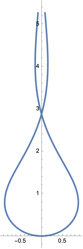
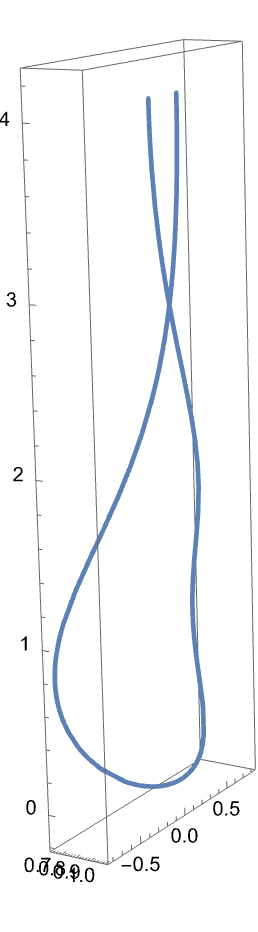
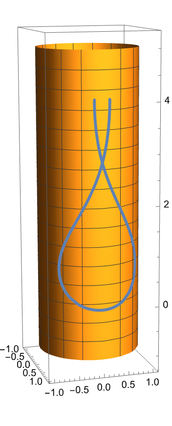
Figure 2. Generating curves of rotational $V$-solitons. Left: the curve $\beta$. Middle and right: projection of the generating curve $\alpha$ on the $xzt$-space (middle) and showing it as subset of the cylinder $\mathbb{S}^{1}\times\mathbb{R}$ (right).

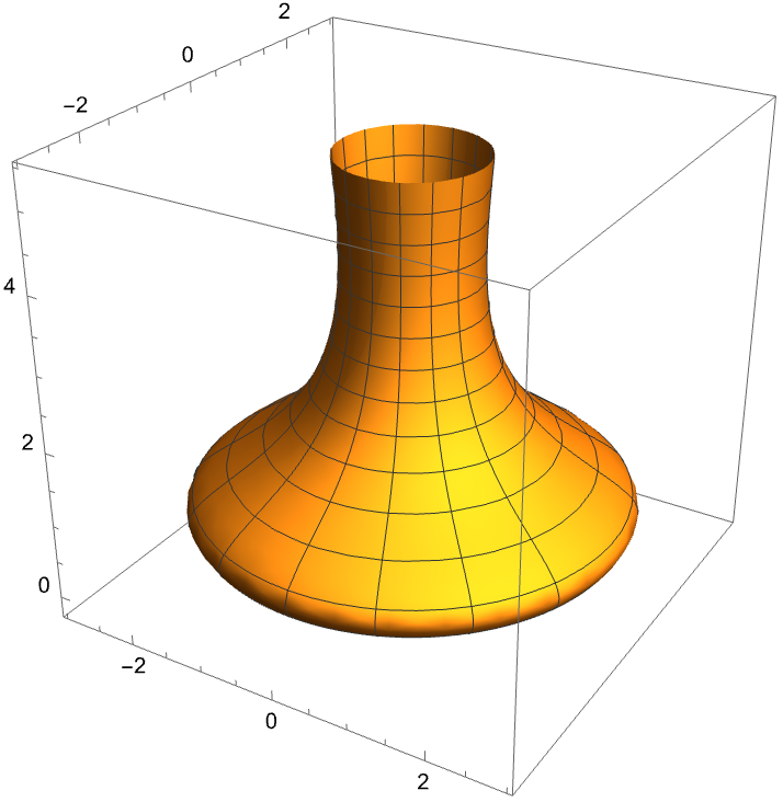
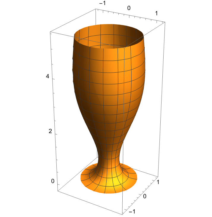
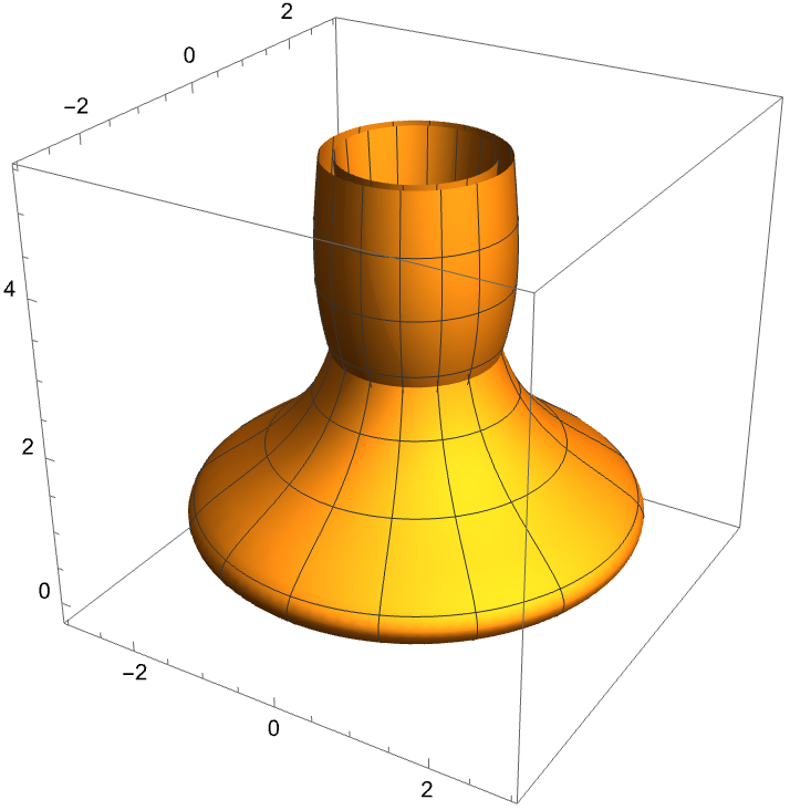
Figure 3. A rotational $V$-soliton after the stereographic projection $p_{r}$. The surface after rotating $\beta$ in the interval $[0,\infty)$ (left) and in the interval $(-\infty,0]$ (middle). Right: the full surface.

Theorem 3.4.

Let $\Sigma$ be a rotational $V$-soliton. Then $\Sigma$ is the cylinder $\mathcal{C}$ or $\Sigma$ is parametrized by (5) with the following properties:

1. The curve $\beta(s)=(u(s),v(s))$ has self-intersections and it is asymptotic to the $v$-axis at infinity. In case that $\beta$ satisfies the initial conditions (17), then $\beta$ is a symmetric bi-graph on the $v$-axis.

2. The surface $\Sigma$ is not embedded with infinitely many intersection points with the $z$-axis.

3. The surface $\Sigma$ is asymptotic to the cylinder $\mathcal{C}$.

In Fig. 3 we show the surface $\Sigma$ after a stereographic projection $p_{r}$ of the first factor $\mathbb{S}^{2}$ into $\mathbb{R}^{2}$, $p_{r}\colon\mathbb{S}^{2}\times\mathbb{R}\to\mathbb{R}^{2}\times\mathbb{R}$, $p_{r}(x,y,z,t)=(\frac{x}{1-z},\frac{y}{1-z},t)$.

4. The class of $R$-solitons

In this section we study $R$-solitons, where the vector field $R$ is

$$R=-y\partial_{x}+x\partial_{y}.$$ (18)

Following our scheme, we will classify $R$-solitons that are vertical surfaces and next, rotational surfaces. First, suppose that $\Sigma$ is a vertical $R$-soliton. We know that $\Sigma$ is parametrized by (3) and that the generating curve $\alpha$ is contained in $\mathbb{S}^{2}$, see (2). A first example of vertical $R$-soliton is a vertical cylinder over the geodesic $\mathbb{S}^{1}\times\{0\}$ of $\mathbb{S}^{2}$. To be precise, let $(u(s),v(s))=(0,s)$. Then $\alpha(s)=(\cos s,\sin s,0)$ in (2) and the surface is the vertical cylinder over $\alpha$ which we have denoted by $\mathcal{C}$ in the previous section. This surface is minimal and it is immediate that $N$ is orthogonal to $R$. Thus $\mathcal{C}$ is a $R$-soliton. Recall that $\mathcal{C}$ is also a rotational $V$-soliton.

Proposition 4.1.

Suppose that $\Sigma$ is a vertical surface parametrized by (3). Then $\Sigma$ is a $R$-soliton if and only if the generating curve $\alpha$ satisfies

$$\left\{\begin{split}u^{\prime}&=\cos u\cos\theta\\ v^{\prime}&=\sin\theta\\ \theta^{\prime}&=\sin\theta\sin u+(\cos u)^{2}\cos\theta.\end{split}\right.$$ (19)

Proof.

The expression of the unit normal $N$ is given in (3). Thus

$$\langle N,R\rangle=-\cos u\cos\theta.$$

Since the expression of $H$ is given in (7), then Eq. (1) is $\theta^{\prime}=\sin\theta\sin u+(\cos u)^{2}\cos\theta$, proving the result. ∎

As in the previous section, we project the solutions of (19) on the $(u,\theta)$-plane, obtaining the autonomous system

$$\left\{\begin{split}u^{\prime}&=\cos u\cos\theta\\ \theta^{\prime}&=\sin\theta\sin u+(\cos u)^{2}\cos\theta.\end{split}\right.$$ (20)

Equilibrium points are $(u,\theta)=(0,\pm\pi/2)$ again, together the points $(u,\theta)=(\pm\frac{\pi}{2},0)$ and translations of length $\pi$ of these points in the $\theta$ variable. For the points $(u,\theta)=(0,\pm\pi/2)$, we have $u(s)=0$ and $v(s)=\pm s$ are solutions. In this case, we know that $\Sigma$ is the vertical cylinder $\mathcal{C}$. The points $(u,\theta)=(\pm\frac{\pi}{2},0)$ do not correspond with surfaces because regularity is lost. In fact, coming back to the parametrization (3), the map $\Psi$ is the parametrization of the vertical fiber at $(0,0,1)\in\mathbb{S}^{2}$.

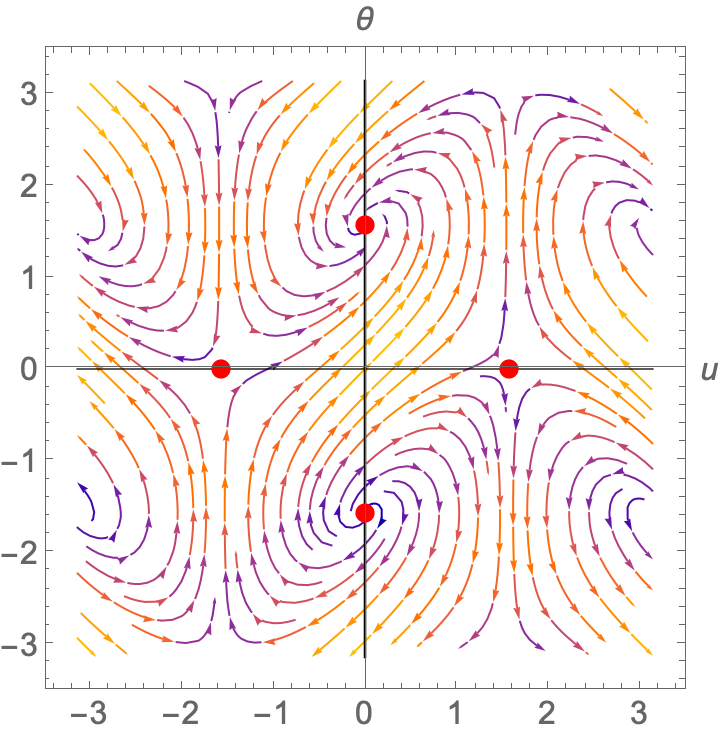
Figure 4. The $(u,\theta)$-phase plane of (20). The red points are the equilibrium points $(0,\pm\frac{\pi}{2})$.

The phase plane is the set $A=(-\pi,\pi)\times(-\pi,\pi)$ in the $(u,\theta)$-plane by the periodicity of $\theta$. If we now compute the linearized system at the points $(u,\theta)=(0,\pm\frac{\pi}{2})$, we find that they have the same character that the ones of the system (15). Thus we have that $(u,\theta)=(0,\frac{\pi}{2})$ is a stable spiral and $(u,\theta)=(0,-\frac{\pi}{2})$ is an unstable spiral.

For the points $(\frac{\pi}{2},0)$ and $(-\frac{\pi}{2},0)$, the linearized system is

$$\left(\begin{array}[]{ll}-1&0\\ 0&1\end{array}\right),\quad\left(\begin{array}[]{ll}1&0\\ 0&-1\end{array}\right),$$

respectively. Since the eigenvalues are two real numbers with opposite signs, then both equilibrium points are saddle points. See Fig. 4. However, this does not affect to the reasoning since the arguments now are similar as in the proof of Thm. 3.4. We omit the details. Figure 5 shows generating curves of vertical $R$-solitons.

Theorem 4.2.

Let $\Sigma$ be a vertical $R$-soliton. Then $\Sigma$ is the cylinder $\mathcal{C}$ or $\Sigma$ is parametrized by (3) with the following properties:

1. The curve $\beta(s)=(u(s),v(s))$ has self-intersections and it is asymptotic to the $v$-axis at infinity. In case that $\beta$ satisfies the initial conditions (17), then $\beta$ is a symmetric bi-graph on the $v$-axis.

2. The surface $\Sigma$ is not embedded with infinitely many intersection points with the $z$-axis.

3. The surface $\Sigma$ is asymptotic to the cylinder $\mathcal{C}$.

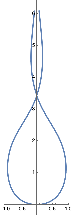
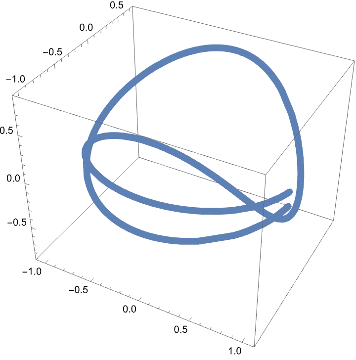
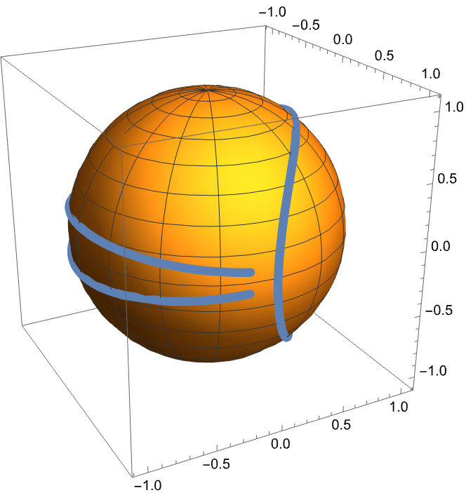
Figure 5. Generating curves of vertical $R$-solitons. Left: solution curve $\beta(s)=(u(s),v(s))$. Middle: the generating curve $\alpha$. Right: the generating curve $\alpha$ contained in the unit sphere $\mathbb{S}^{2}$.

The second type of $R$-solitons are those surfaces that are invariant by a one-parameter group of rotations of the first factor. Since we have defined in (18) the vector field $R$ as the rotation about the direction $(0,0,1)\in\mathbb{S}^{2}$, we cannot a priori fix the rotational axis of the surface.

Theorem 4.3.

The only rotational $R$-solitons are:

1. Slices $\mathbb{S}^{2}\times\{t_{0}\}$, $t_{0}\in\mathbb{R}$, viewed as rotational surfaces with respect to any axis of $\mathbb{S}^{2}$ and;

2. Rotational minimal surfaces about the $z$-axis.

Proof.

Let $\Sigma$ be a rotational $R$-soliton. In order to have manageable computations of the mean curvature $H$ and the unit normal $N$ of $\Sigma$, we will assume in this proof that the rotation axis of $\Sigma$ is the $z$-axis. Thus we are assuming that the surface is parametrized by (5). Thus the vector field $R$ is now arbitrary and with no a priori relation with the $z$-axis. The vector field $R$ is determined by an orthonormal basis $B=\{E_{1},E_{2},E_{3}\}$ of $\mathbb{R}^{3}$. With respect to $B$, the vector field $R$ can be expressed by

$$R(x_{1},x_{2},x_{3},t)=-x_{2}E_{1}+x_{1}E_{2},$$

where $(x_{1},x_{2},x_{3})$ are coordinates of $\mathbb{S}^{2}$ with respect to $B$.

We now write $E_{1}$ and $E_{2}$ with respect to the canonical basis of $\mathbb{R}^{3}$,

$$E_{i}=(\cos m_{i}\sin n_{i},\cos m_{i}\sin n_{i},\sin m_{i}),\quad i=1,2,$$

where $m_{i},n_{i}\in\mathbb{R}$. The unit normal $N$ and the mean curvature $H$ of $\Sigma$ were computed in (10) and (11), respectively. Then

$$\begin{split}\langle N,R\rangle&=-\langle\Psi,E_{2}\rangle\langle N,E_{1}\rangle+\langle\Psi,E_{1}\rangle\langle N,E_{2}\rangle\\ =&(\sin m_{1}\cos m_{2}\sin n_{2}-\cos m_{1}\sin n_{1}\sin m_{2})\sin\theta\sin\varphi\\ &+(\sin m_{1}\cos m_{2}\cos n_{2}-\cos m_{1}\cos n_{1}\sin m_{2})\sin\theta\cos\varphi.\end{split}$$ (21)

Looking now Eq. (1), we have that in the expression of right hand-side of (1), that is, $\langle N,R\rangle$, formula (21), the variable $\varphi$ do appear. However in the left hand-side of (1), the mean curvature $H$, formula (11), does not depend on $\varphi$. This implies that the coefficients of $\sin\varphi$ and $\cos\varphi$ in (21) must vanish. Both coefficients contain the factor $\sin\theta$. This gives the following discussion of cases.

1. Case $\sin\theta(s)=0$ for all $s$. Then $u(s)=s$ and $v(s)$ is a constant function, $v(s)=t_{0}$, $t_{0}\in\mathbb{R}$. This proves that $\Sigma$ is a slice $\mathbb{S}^{2}\times\{t_{0}\}$.

2. Case $\sin\theta(s_{0})\not=0$ at some $s_{0}$. Then in an interval around $s=s_{0}$, we deduce

   $$\sin m_{1}\cos m_{2}\sin n_{2}-\cos m_{1}\sin n_{1}\sin m_{2}=0,$$

   $$\sin m_{1}\cos m_{2}\cos n_{2}-\cos m_{1}\cos n_{1}\sin m_{2}=0.$$

   Both identities imply $E_{1}\times E_{2}=(0,0,1)$. Thus $R$ coincides with the vector field defined in (18) and the rotation axis is the $z$-axis. Moreover, the right hand-side of (1) is $0$, proving that the surface is minimal. This proves the result.

∎

Minimal surfaces in $\mathbb{S}^{2}\times\mathbb{R}$ of rotational type with respect to an axis in the first factor were classified by Pedrosa and Ritoré [12].

References

- [1] A. Bueno, Translating solitons of the mean curvature flow in the space . J. Geom. 109 (2018), 42.
- [2] A. Bueno, Uniqueness of the translating bowl in . J. Geom. 11 (2020), 43.
- [3] A. Bueno, R. López, A new family of translating solitons in hyperbolic space. arXiv:2402.05533v1 [math.DG] (2024).
- [4] A. Bueno, R. López, Horo-shrinkers in the hyperbolic space. arXiv:2402.05527 [math.DG] (2024).
- [5] A. Bueno, R. López, The class of grim reapers in . arXiv:2402.05772 [math.DG] (2024).
- [6] G. Huisken, C. Sinestrari, Convexity estimates for mean curvature flow and singularities of mean convex surfaces. Acta Math. 183 (1999), 45–70.
- [7] R. F. de Lima, G. Pipoli, Translators to higher order mean curvature flows in and . arXiv:2211.03918v2 [math.DG] (2024).
- [8] R. F. de Lima, A. K. Ramos, J. P. dos Santos, Solitons to mean curvature flow in the hyperbolic 3-space. arXiv:2307.14136 [math.DG] (2023).
- [9] J. de Lira, F. Martín, Translating solitons in riemannian products. J. Differential Equations, 266 (2019), 7780–7812.
- [10] R. López, M. I. Munteanu, Translators in the special lineal group. Submitted, preprint (2024).
- [11] L. Mari, J. Rocha de Oliveira, A. Savas-Halilaj, R. Sodré de Sena, Conformal solitons for the mean curvature flow in hyperbolic space. arXiv:2307.05088 [math.DG] (2023).
- [12] R. Pedrosa, M. Ritoré, Isoperimetric domains in the Riemannian product of a circle with a simply connected space form and applications to free boundary value problems. Indiana Univ. Math. J. 48 (1999), 1357–1394.
- [13] L. Perko, Differential Equations and Dynamical Systems. Springer, New York, 2001.
- [14] G. Pipoli, Invariant translators of the solvable group. Ann. Mat. Pura Appl. 199 (2020), 1961–1978.
- [15] G. Pipoli, Invariant translators of the Heisenberg group. J. Geom. Anal. 31 (2021), 5219–5258.
- [16] H. Rosenberg, Minimal surfaces in . Illinois J. Math. 46 (2001), 1177 – 1195.