Quantum Annealing Inspired Algorithms for Track Reconstruction at High Energy Colliders

Abstract

Charged particle reconstruction or track reconstruction is one of the most crucial components of pattern recognition in high energy collider physics. It is known for enormous consumption of the computing resources, especially when the particle multiplicity is high. This would indeed be the conditions at future colliders such as the High Luminosity Large Hadron Collider and Super Proton Proton Collider. Track reconstruction can be formulated as a quadratic unconstrained binary optimization (QUBO) problem, for which various quantum algorithms have been investigated and evaluated with both the quantum simulator and hardware. Simulated bifurcation algorithms are a set of quantum annealing inspired algorithms, and are serious competitors to the quantum annealing, other Ising machines and their classical counterparts. In this study, we show that the simulated bifurcation algorithms can be employed for solving the particle tracking problem. As the simulated bifurcation algorithms run on classical computers and are suitable for parallel processing and usage of the graphical processing units, they can handle significantly large data at high speed. These algorithms exhibit compatible or sometimes improved reconstruction efficiency and purity than the simulated annealing, but the running time can be reduced by as much as four orders of magnitude. These results suggest that QUBO models together with the quantum annealing inspired algorithms are valuable for the current and future particle tracking problems.

• February 2024

Keywords: quantum algorithm, quantum annealing, simulated bifurcation, Ising problem, particle tracking, pattern recognition, LHC

1 Introduction

High energy colliders have been playing important roles in particle physics, discovering new particles and precisely measuring its interactions and properties. The Higgs boson, the last missing piece of the Standard Model, was discovered in 2012 at the Large Hadron Collider (LHC) at European Organization for Nuclear Research (CERN) by the ATLAS and CMS experiments [1, 2]. The LHC has been successfully operating since 2009, and will be upgraded to the High Luminosity LHC (HL-LHC) [3] scheduled to start after 2029 with an increased luminosity by several factors from the current LHC Run 3 operation. The event rate will also increase by a factor of 10 due to the trigger upgrade. The HL-LHC will collect over 10 times the data recorded at the LHC, leading to about 180 million Higgs bosons produced. This will allow us to measure the Higgs sector in an unprecedented precision. With such an enormous amount of data collected and increase in the data size by a factor of four to five due to the new detector, it will bring the LHC from the current peta-byte data operation to the “Exa-byte” era. The HL-LHC is expected to be followed by future colliders such as the Circular Electron Positron Collider (CEPC) [4, 5, 6] and Super Proton-Proton Collider (SppC) [7, 8] to be hosted in China as well as similar projects under consideration in the world.

Charged particle reconstruction, track reconstruction or tracking in short, is one of the most crucial components of reconstruction and the highest CPU-consuming reconstruction task at the LHC. It is a patter recognition procedure to recover charge particle trajectories from hits in the inner-most detector, fully composed of silicon layers at the HL-LHC, for example. As the trajectories are bent by the solenoid magnetic field, measuring their curvature will provide momenta of the particles. The number of reconstructed tracks per event at the LHC has been at the order of hundreds, but will increase by an order of magnitude at the HL-LHC, reaching about ten thousand tracks at most. The required computing time increases exponentially against the luminosity [9, 10, 11], and various innovations are urgently needed to overcome this challenge.

The Kalman Filter technique [12] has been used as a standard algorithm at the LHC, and is also implemented in an open-source project called A Common Tracking Software (ACTS) [13]. The Kalman Filter initiates seeding from the inner layers of the tracking detector, and the tracks are extrapolated to find the next hit in outer layers. The track fit is iterated to find the best quality among the hit combinations. Its highly efficient track reconstruction and very low misidentification rate have made the Kalman Filter to remain as the key player for the tracking. However, due to its iterative process, the computing time will grow exponentially against the track multiplicity.

To cope with this challenge, machine learning methods such as the graph neural network (GNN) are actively being investigated at the LHC [14, 15] and Beijing Spectrometer (BES) III [16], the tau-lepton and charm quark factory in China. The nodes of the graphs represent hits in the silicon detector, and the edges represent segments obtained by connecting those silicon hits. The GNN-based approaches provide compatible track reconstruction performance as the Kalman Filter, but the computing time scales approximately linearly.

Applications of quantum computing and algorithms are yet another trend of innovative approaches being investigated to cope with the track reconstruction in the dense conditions. The first such studies [17, 18] utilized the quantum annealing computer, considering the track reconstruction as a quadratic unconstrained binary optimization (QUBO) problem. Modeling track reconstruction as a QUBO problem and solving it by a simulated annealing actually goes back to the time of the ALEPH experiment [19]. However, the experimental condition of low track multiplicity and the non-demanding computing load at that time are significantly different from the current LHC and future HL-LHC, and thus several modifications were necessary, as was implemented in Refs. [17, 18]. In the past few years, several groups have also investigated the possibility to use the quantum gate simulators and computers instead [20, 21, 22, 23, 24, 25]. With the quantum gates, a QUBO can be mapped to an Ising Hamiltonian and be solved using Variational Quantum Eigensolver (VQE), Quantum Approximate Optimization Algorithm (QAOA), or similar variants. Recently, introducing the GNN tracking in the quantum gate computers [26] or in the quantum annealing machines [27] is also being proposed. There is also a conceptual study categorizing the track reconstruction into four routines and demonstrate how the quantum advantage can be achieved [28].

2 Methodology

Track reconstruction can be regarded as an Ising problem. It is an NP (Nondeterministic Polynomial time) complete problem, in which the solution candidates diverge exponentially with the problem size. Machines dedicated to solve such a class of problems are called the Ising machines. The quantum annealer by D-Wave [29] based on the quantum annealing concept [30] and the coherent Ising machine (CIM) [31] are such examples.

In 2016, a new quantum computer modifying the CIM, the quantum bifurcation machine (QbM) [32, 33] was proposed. The classical version of QbM, the classical bifurcation machine (CbM), was also introduced in parallel [32, 33]. This classical algorithm no longer has the foundation of quantum adiabatic theorem but can still find quasi-optimal solutions. The original equation of motion of CbM was then modified to speed up the numerical simulation, and is called the simulated bifurcation (SB) [34]. This quantum annealing inspired algorithm (QAIA) is found to be suitable for parallel computing and expected to outperform the CIM. The details of the SB, the simulated annealing (SA) [35] considered as the benchmark of this study, and how the track reconstruction is formulated as an Ising or QUBO problem are mentioned below. The simulated CIM [36] showed visibly degraded performance for the track reconstruction in terms of both predicting the minimum Ising energy and speed to obtain an answer, thus not presented in this work.

2.1 Simulated bifurcation

The first SB proposed, the adiabatic SB (aSB), is formulated as:

$$\centering\dot{x}_{i}\@add@centering = \frac{\partial H_{\textrm{aSB}}}{\partial y_{i}}=a_{0}y_{i}$$ (1)

$$\dot{y}_{i} = -\frac{\partial H_{\textrm{aSB}}}{\partial x_{i}},$$ (2)

$$= -\left[x_{i}^{2}+a_{0}-a(t)\right]x_{i}+c_{0}\sum_{j=1}^{N}J_{i,j}x_{j},$$

$$H_{\textrm{aSB}} = \frac{a_{0}}{2}\sum_{i=1}^{N}y_{i}^{2}+V_{\textrm{aSB}}$$ (3)

$$V_{\textrm{aSB}} = \sum_{i=1}^{N}\left(\frac{x_{i}^{4}}{4}+\frac{a_{0}-a(t)}{2}x_{i}^{2}\right)$$ (4)

$$-\frac{c_{0}}{2}\sum_{i=1}^{N}\sum_{j=1}^{N}J_{i,j}x_{i}x_{j},$$

where $x_{i}$ and $y_{i}$ are respectively the position and momentum of a particle for the $i$-th spin, $a(t)$ is a time-dependent control parameter monotonically increased from zero, $a_{0}$ and $c_{0}$ are positive constants, $H_{\textrm{aSB}}$ is the Hamiltonian, and $V_{\textrm{aSB}}$ is the potential energy in aSB. The numerical computation is pursued with the symplectic Euler method [37]. All the positions and momenta can be instantaneously updated, thus this method is suited for parallel computation, which is a notable difference from the simulated annealing.

Despite the above mentioned appealing characteristics, the precision of aSB was found to be problematic, and a few variants of the algorithm were proposed [38]. The degradation of aSB performance mostly originates from the fact that it treats the discrete values of the spins as the continuous variables $x_{i}$. The ballistic simulated bifurcation algorithm (bSB) introduces complete inelastic scattering walls at $|x_{i}|>1$, meaning that $x_{i}$ is forced to be at $x_{i}=\pm 1$ and $y_{i}=0$ when it passed the threshold. The equation of motion is formulated as below:

$$\centering\dot{x}_{i}\@add@centering = \frac{\partial H_{\textrm{bSB}}}{\partial y_{i}}=a_{0}y_{i}$$ (5)

$$\dot{y}_{i} = -\frac{\partial H_{\textrm{bSB}}}{\partial x_{i}},$$ (6)

$$= -\left[a_{0}-a(t)\right]x_{i}+c_{0}\sum_{j=1}^{N}J_{i,j}x_{j},$$

$$H_{\textrm{bSB}} = \frac{a_{0}}{2}\sum_{i=1}^{N}y_{i}^{2}+V_{\textrm{aSB}}$$ (7)

$$V_{\textrm{bSB}} = \frac{a_{0}-a(t)}{2}\sum_{i=1}^{N}x_{i}^{2}$$ (8)

$$-\frac{c_{0}}{2}\sum_{i=1}^{N}\sum_{j=1}^{N}J_{i,j}x_{i}x_{j},$$

$$\quad~{}(\textrm{when}~{}|x_{i}|\leq 1~{}\textrm{for all}~{}x_{i}),$$

$$= \infty~{}(\textrm{otherwise}).$$

As the potential wall is introduced at $x_{i}=1$, the quartic term is removed to avoid the divergence. In addition to the precision, the bSB is found to be about 12 times faster than the aSB when implemented in Field Programmable Gate Array (FPGA) [38].

The discrete simulated bifurcation (dSB) partially introduces discretization of the position in the equation of motion, replacing $x_{i}$ by $\textrm{sgn}(x_{i})$. This approach is expected to reduce the analog error. More interestingly, due to the violation of energy conservation from the discretization, it shows a pseudo-quantum-tunneling behavior. Its equation of motion is written as below:

$$\centering\dot{x}_{i}\@add@centering =\frac{\partial H_{\textrm{dSB}}}{\partial y_{i}}=a_{0}y_{i}$$ (9)

$$\dot{y}_{i} =-\frac{\partial H_{\textrm{dSB}}}{\partial x_{i}},$$ (10)

$$=-\left[a_{0}-a(t)\right]x_{i}+c_{0}\sum_{j=1}^{N}J_{i,j}\textrm{sgn}(x_{j}),$$

$$H_{\textrm{dSB}} =\frac{a_{0}}{2}\sum_{i=1}^{N}y_{i}^{2}+V_{\textrm{aSB}}$$ (11)

$$\centering V_{\textrm{dSB}}\@add@centering =\frac{a_{0}-a(t)}{2}\sum_{i=1}^{N}x_{i}^{2}$$ (12)

$$-\frac{c_{0}}{2}\sum_{i=1}^{N}\sum_{j=1}^{N}J_{i,j}x_{i}\textrm{sgn}(x_{j}),$$

$$\qquad~{}~{}(\textrm{when}~{}|x_{i}|\leq 1~{}\textrm{for all}~{}x_{i})$$

$$=\infty~{}~{}(\textrm{otherwise}),$$

where the above-mentioned partial discretization is introduced by replacing some $x_{i}$ by $\textrm{sgn}(x_{i})$.

Another set of variants introducing heat fluctuations [39] is not considered in this study, as it did not bring in significant improvement in the results. The SB algorithms are implemented in Huawei MindSpore Quantum [40] and are adopted in this study. The aSB is already significantly outperformed by the other variants and is not considered. A recent application of the SB algorithms to drug designs is documented in Ref. [41].

2.2 Simulated Annealing

In this work, the simulated annealing algorithm implemented in D-Wave Neal [42] is considered as the baseline to compare to, as its performance on the tracking is already known and presented in a previous study [17, 43]. The D-Wave Neal is based on the method proposed in Ref. [35]. It utilizes random moves in the solution space to search for the global minimum. In analogy to finding ground states of matter, a “temperature” is introduced, first by “melting” a substance by a high temperature and slowly lowering it until the system “freezes”, just as growing a crystal from a melt. The iteration is pursued with a simple algorithm proposed in Ref. [44], where a small random displacement is applied to the original spin configuration, and its energy difference $\Delta E$ is computed. If $\Delta E<0$, the new configuration is accepted as the new temporary prediction and move on to the next iteration. If $\Delta E>0$, the new configuration is accepted only probabilistically from the Boltzmann factor: $P(\Delta E)=\exp(-\Delta E/k_{B}T)$.

Another QUBO solver qbsolv [45] provided by D-Wave utilizes a sub-QUBO method, which partitions the original QUBO matrix into pieces. Those smaller sub-problems are then solved using a classical solver running the tabu algorithm [46]. Sub-QUBO methods are mainly motivated for the implementation in the actual quantum annealing hardware, which has limitations to the problem size due to the available number of qubits. Speed of qbsolv is more than two orders of magnitude slower than Neal with no gain in performance on the track reconstruction [17, 43]. Thus, it is not considered in our study.

2.3 Track reconstruction and QUBO formulation

To reconstruct the tracks, hits in the silicon detectors are connected, starting from doublets: segments of two silicon hits. Then, triplets, segments of three silicon hits, are created by connecting the doublets. Triplets are connected to reconstruct the final tracks, by evaluating the consistency of the triplet momenta. The following formulation of a QUBO considered in Refs. [17, 23, 24, 43, 47] is adopted:

$$O(a,b,T)=\sum_{i=1}^{N}a_{i}T_{i}+\sum_{i=1}^{N}\sum_{j<i}^{N}b_{ij}T_{i}T_{j},$$ (13)

where $N$ is the number of triplets, $T_{i}$ and $T_{j}$ correspond to the triplets and take the value of either zero or one, $a_{i}$ are the bias weights to evaluate the quality of the triplets, and $b_{ij}$ are the coefficients that quantify the compatibility of two triplets ($b_{ij}=0$ if no shared hit, $=1$ if there is any conflict, and $=-S_{ij}$ if two hits are shared between the triplets). The coefficients $-S_{ij}$ quantify the consistency of the two triplet momenta by [17]:

$$S_{ij}=\frac{1-\frac{1}{2}(|\delta(q/p_{Ti},q/p_{Tj})|+max(\delta\theta_{i},\delta\theta_{j}))}{(1+H_{i}+H_{j})^{2}},$$ (14)

where $\delta$ is the difference between the curvature $q/p_{T}$ or angle $\theta$ of the two triplets and $H_{i}$ is the number of holes in the triplet. The bias weights $a_{i}$ have significant impact on the Hamiltonian energy landscape and thus on the track reconstruction, in particular its purity (defined in Sec. 4), and computation speed. They can be parameterized as:

$$a_{i}=\alpha\left(1-e^{\frac{\mid d_{0}\mid}{\gamma}}\right)+\beta\left(1-e^{\frac{\mid z_{0}\mid}{\lambda}}\right),$$ (15)

where $d_{0}$ and $z_{0}$ are the transverse and longitudinal displacements of the triplets from the primary vertex (the most significant proton-proton collision point in an event) and $\alpha$, $\beta$, $\gamma$ and $\lambda$ are tunable parameters, which are taken to be 0.5, 0.2, 1.0 and 0.5, optimized in a previous study [43] for the same dataset as described in the next section.

3 Dataset

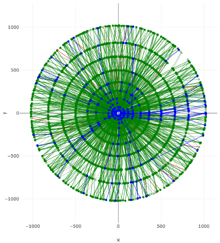
Figure 1: Display of the highest particle multiplicity event in the dataset. The green (red) lines indicate correctly (incorrectly) reconstructed tracks, whereas the blue lines are the ones not reconstructed. This display is generated with the hepqpr-qallse framework [48].

An open source dataset from the TrackML Challenge is used [49, 50]. The events contain a top quark pair generated with Pythia8 [51] event generator overlaid with additional 200 proton-proton interactions compatible with the HL-LHC conditions. A generalized full silicon tracker called the TML detector, mimicking the inner detector component of the ATLAS experiment for the HL-LHC condition, is considered. The detector consists of three detector volumes, cylindrical in the barrel (central) region and multiple disks in the end-cap (side) region. Each detector volume has several silicon layers, leading to 10 layers in total for the whole TML detector. However, the dataset is simplified by focusing on the barrel region of the detector, namely removing the hits in the end-cap region. This approach is often adopted for tracking studies for the HL-LHC.

A fast detector simulation implemented in the ACTS software is applied to the charged particles traversing the silicon layers. The solenoid magnetic field of 2T with realistic inhomogeneous distortion of the field strength is considered. The material interactions such as the multiple scattering, energy loss and hadronic interactions are parameterized in the simulation. Inefficiency in the silicon sensors, false silicon hits as well as production of secondary particles from the detector material are also considered. Figure 1 shows an event display from the highest particle multiplicity event in the dataset. It clearly demonstrates how dense the reconstructed tracks are under the HL-LHC condition.

4 Results

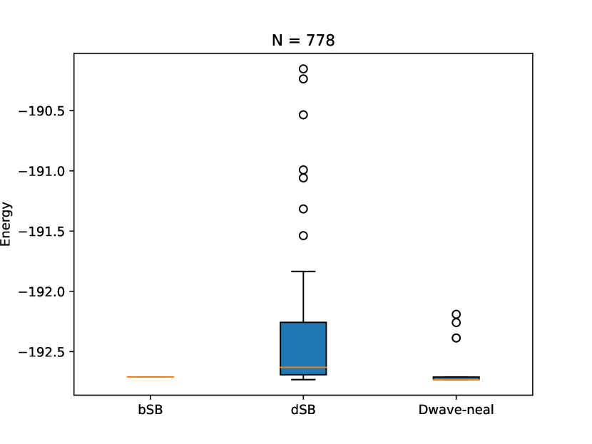
(a)

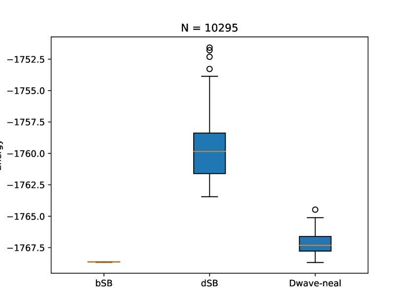
(b)

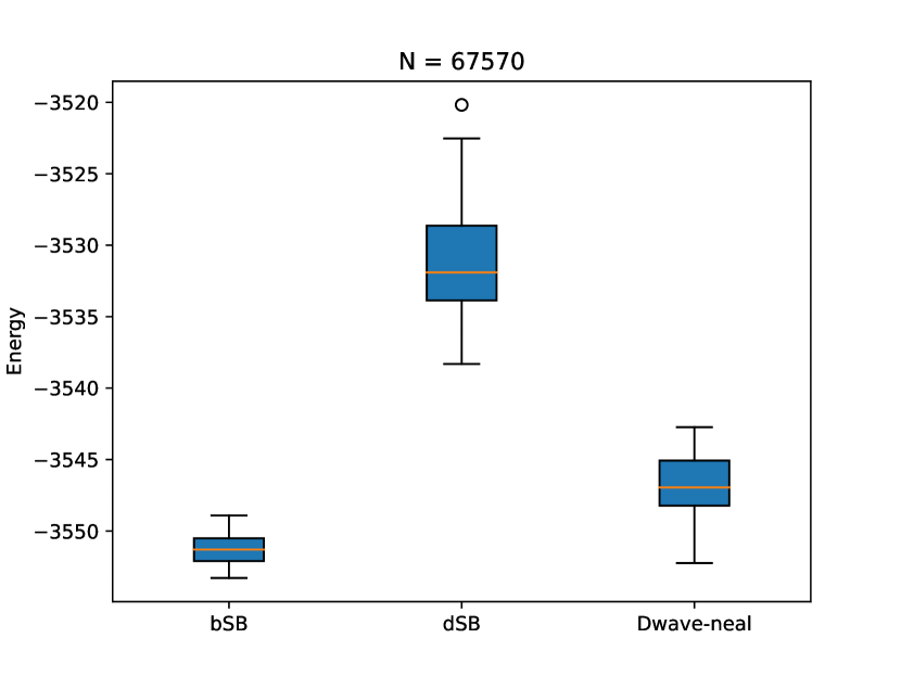
(c)

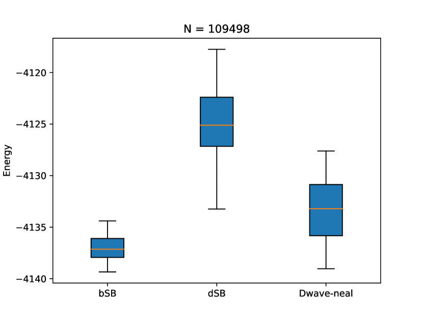
(d)

Figure 2: Minimum Ising energy estimated by various QAIAs. Four examples with the full QUBO size of 778$\times$778 [409 particles] (a), 10295$\times$10295 [4092 particles] (b), 67570$\times$67570 [8187 particles] (c) and 109498$\times$109498 [9435 particles] (d) are presented.

First of all, performance of the three QAIAs: bSB, dSB and D-wave Neal is evaluated by the predicted minimum Ising energy and its stability over 50 shots. For the bSB and dSB, the parameter $a_{0}$ in Eqs. (6) and (10) and the time step $\Delta t$ are set to be 1, as similar to the proposed values in Ref. [38]. Two approaches have been tested for the parameter $c_{0}$, the former keeping it as fixed and the latter pursuing an automatic optimization scan. There is no significant difference in performance for both cases, thus the results are presented for the fixed $c_{0}$ parameter case onwards. As shown in Figure 2, the bSB provides the lowest predicted minimum energy with the smallest fluctuation regardless of the QUBO size, followed by Neal. The dSB tends to have slightly degraded energy prediction with larger fluctuation, though its impact is not critical on the final track reconstruction performance, as will be presented below.

Actual performance of the track reconstruction is evaluated in terms of the efficiency and purity; or the recall and precision in the data science terminology. They are defined as below:

$$\mathrm{Efficiency~{}(Recall)}=\frac{TP}{TP+FN},$$ (16)

$$\centering\mathrm{Purity~{}(Precision)}=\frac{TP}{TP+FP},\@add@centering$$ (17)

where $TP$ is the true positive, $FN$ the false negative, and $FP$ the false positive. $TP$ corresponds to the number of reconstructed doublets matching to the correct (true) doublets. $FN$ is the number of true doublets that are not reconstructed, thus $TP+FN$ is simply the number of true doublets. $FP$ is the number of reconstructed doublets that do not match to the true doublets, namely the “fake” doublets in the high energy physics terminology. Figure 3 shows the efficiency and purity for the three QAIA cases. The statistical uncertainty and the root-mean-square of the fluctuations from 50 shots are added in quadrature and presented in the figure. The statistical uncertainty is a few times larger than the fluctuations from 50 shots, thus the latter effect is not significant for all the three algorithms. Excellent efficiency of above 95% is obtained throughout the whole dataset up to the highest particle multiplicity of about 10000 for all the algorithms. The purity decreases with the particle multiplicity, but stays to be above 84% for all the events and above 95% for events with the particle multiplicity less than 6000. The dSB tends to have slightly lower performance, though mostly within the statistical uncertainty. An event display from the highest multiplicity event reconstructed with the bSB is presented in Figure 1.

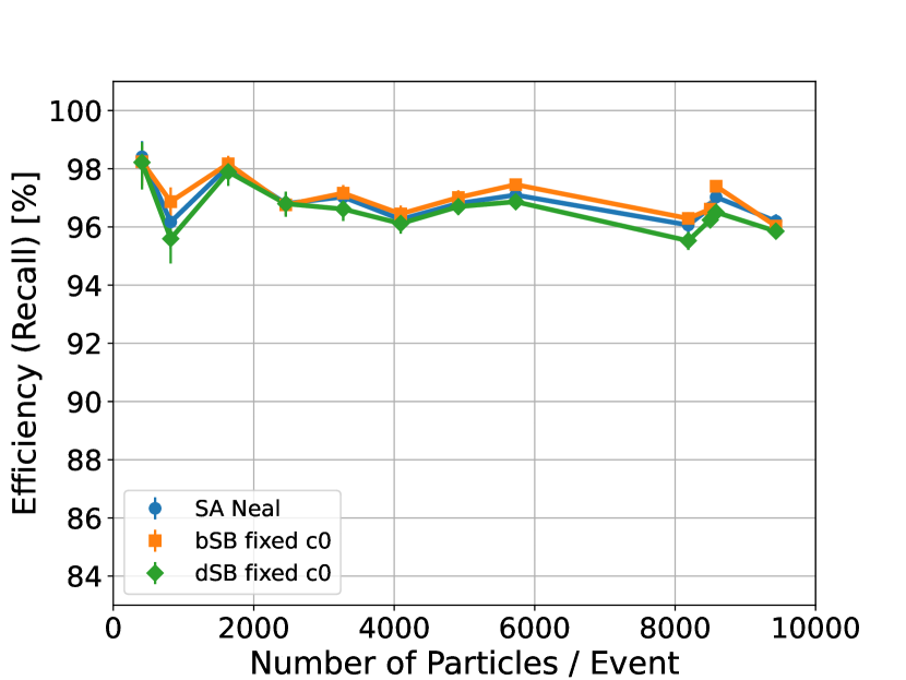
(a)

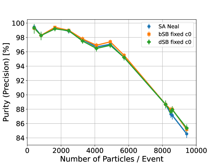
(b)

Figure 3: Efficiency (recall) (a) and purity (precision) (b) as a function of particle multiplicity evaluated for the three QAIA algorithms.

Finally, the execution time is evaluated for each algorithm on an AMD EPYC 7642 CPU and an NVIDIA A100 GPU. Figure 4 presents the evolution of Ising energies evaluated for the three QAIAs. The average of the 50 shots as well as the envelopes from the best and worst cases are shown in the figure. Usage of the GPU is generally not effective for the simulated annealing algorithms due to the lack of parallelizability of the spin update, and thus the GPU option is not provided for the D-Wave Neal.

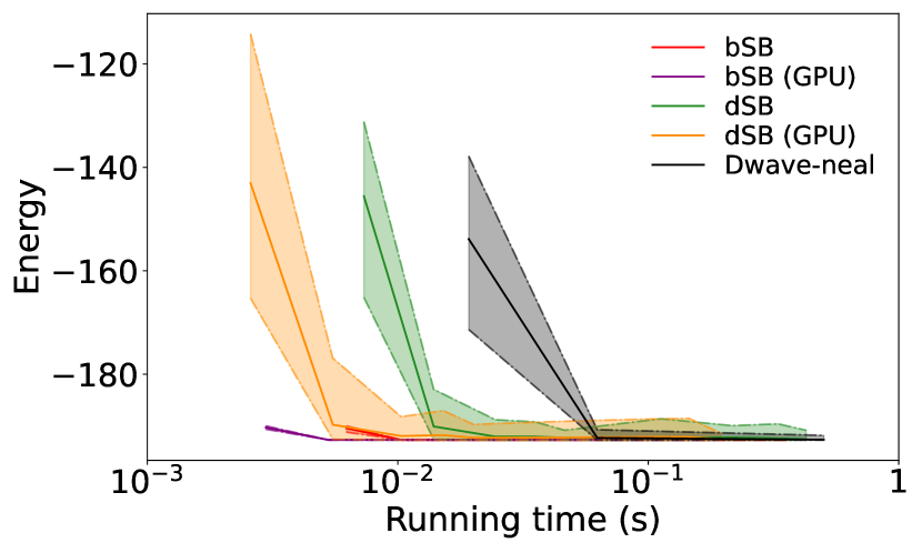
(a)

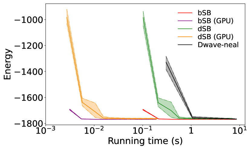
(b)

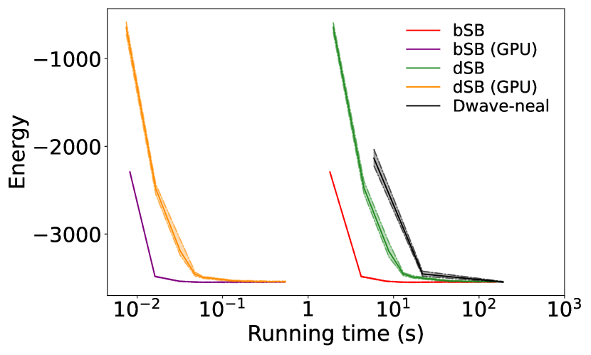
(c)

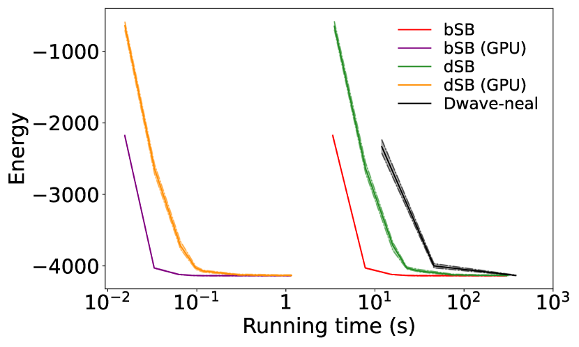
(d)

Figure 4: The evolution of Ising energies evaluated for the three QAIA algorithms. Four examples with the full QUBO size of 778$\times$778 [409 particles] (a), 10295$\times$10295 [4092 particles] (b), 67570$\times$67570 [8187 particles] (c) and 109498$\times$109498 [9435 particles] (d) are presented. The solid lines indicate the average from the 50 shots, whereas the envelopes represent the best and worst cases among those shots.

More quantitative computation speed is summarized in Table 1 using the time-to-target (TTT) metric [52]. The time-to-solution (TTS) metric [53, 54] is more standard when evaluating the Ising machine speed, but it requires the true ground state to be known. As the true ground state is unknown in our dataset, the TTT is adopted, where the target value is set to 99.9% of the lowest energy value obtained from our study. We adopted TTT to be the time required to find the target value with the 99% probability. For small-size QUBOs, the bSB is one order of magnitude faster than the D-Wave Neal. The impact of the GPU usage becomes significant for large-size QUBOs, leading to four orders of magnitude speed-up for the highest multiplicity event compared to the D-Wave Neal. The dSB was not able to reach 99.9% of the target value for larger datasets. If the target requirement is loosened, the speed of dSB is generally faster by a few factors with the CPU and faster by two to three orders of magnitude with the GPU compared to the D-Wave Neal. The event with 8583 particles shows TTT not following the general trend in regards to the dataset size. This is due to the fact that this event has a lower level of difficulty to solve than the other events. The difficulty to solve a problem largely depends on the graph structure corresponding to the QUBO and its weight distribution.

Data Information		Time to target [s]
# of particles	QUBO size	bSB	bSB (GPU)	dSB	dSB (GPU)	D-Wave Neal
409	778	$0.007\,245\,779$	$0.020\,662\,069$	$0.031\,515\,559$	$0.091\,926\,043$	$0.059\,812\,821$
818	1431	$0.011\,502\,504$	$0.018\,694\,162$	$0.292\,698\,172$	$0.478\,396\,161$	$0.168\,638\,337$
1637	2904	$0.011\,502\,504$	$0.018\,694\,162$	$0.292\,698\,172$	$0.478\,396\,161$	$0.168\,638\,337$
2456	4675	$0.013\,970\,346$	$0.017\,061\,959$	–	–	$0.479\,039\,48$
3274	6945	$0.031\,686\,266$	$0.022\,400\,359$	–	–	$1.229\,060\,412$
4092	10295	$0.005\,215\,515$	$0.021\,833\,923$	$0.014\,852\,901$	$0.064\,933\,106$	$0.029\,895\,86$
4912	14855	$0.027\,419\,039$	$0.016\,360\,553$	–	–	$2.164\,885\,195$
5730	22022	$0.109\,022\,825$	$0.041\,646\,643$	–	–	$3.852\,833\,933$
8187	67570	$0.488\,203\,862$	$0.028\,466\,368$	–	–	$404.296\,791\,6$
8500	78812	$1.899\,454\,457$	$0.107\,649\,927$	–	–	$785.732\,030\,5$
8583	80113	$1.320\,794\,143$	$0.067\,178\,113$	–	–	$93.781\,875\,84$
9435	109498	$3.884\,063\,796$	$0.140\,178\,046$	–	–	$1366.808\,432$

Table 1: Time to target (TTT) for various datasets using the bSB, dSB and D-Wave Neal. Time is not shown if the prediction did not reach the target value.

5 Discussion

Three sets of quantum annealing inspired algorithms are evaluated for track reconstruction formulated as a quadratic unconstrained binary optimization (QUBO) problem. The ballistic simulated bifurcation provides improved performance over the D-Wave Neal simulated annealers in all aspects; for finding the minimum Ising energy with higher stability, compatible or slightly higher performance on the track reconstruction efficiency and purity, and significant speed-up by four orders of magnitude at most. This trend of improvement becomes more and more peculiar as the dataset size increases, which is quite promising for the future colliders such as the High Luminosity Large Hadron Collider and Super Proton Proton Collider. The discrete simulated bifurcation shows slightly degraded prediction of the minimum energy, but its impact is not significant in terms of efficiency and purity of the track reconstruction. It is generally two to three orders of magnitude faster than the D-Wave Neal. The affinity with parallel processing and usage of cutting-edge computing resources make the simulated bifurcation algorithms to be a promising option to be adopted in high energy collider experiments. It is worth emphasizing that these are “quantum-inspired” algorithms running on classical computers. Thus, they are not technologies for the future, but would be a serious option to be adopted for any ongoing collider experiments.

Nevertheless, one thing to note is that the execution time for the QUBO modeling, namely the doublet and triplet formation and preparing a QUBO matrix from each given dataset is not included in the results. This portion of the procedure also takes significant amount of time, but the execution is currently performed on a single CPU [48] and definitely far from being optimized in terms of speed performance. It could be significantly improved with parallel processing and a careful optimization. Its speedup should not be a major bottleneck, but is left for future studies.

References

References

- [1] ATLAS Collaboration. Observation of a new particle in the search for the Standard Model Higgs boson with the ATLAS detector at the LHC. Phys. Lett. B, 716:1–29, 2012.
- [2] CMS Collaboration. Observation of a New Boson at a Mass of 125 GeV with the CMS Experiment at the LHC. Phys. Lett. B, 716:30–61, 2012.
- [3] I. Béjar Alonso, O. Brüning, P. Fessia, M. Lamont, L. Rossi, L. Tavian, M. Zerlauth (editors). High-Luminosity Large Hadron Collider (HL-LHC): Technical design report. CERN Yellow Reports: Monographs. CERN, Geneva, 2020.
- [4] CEPC Study Group. CEPC Technical Design Report – Accelerator. IHEP-CEPC-DR-2023-01, IHEP-AC-2023-01, 12 2023.
- [5] CEPC Study Group. CEPC Conceptual Design Report: Volume 1 - Accelerator. IHEP-CEPC-DR-2018-01, IHEP-AC-2018-01, 2018.
- [6] CEPC Study Group. CEPC Conceptual Design Report: Volume 2 - Physics & Detector. IHEP-CEPC-DR-2018-02, IHEP-EP-2018-01, IHEP-TH-2018-01, 2018.
- [7] CEPC-SPPC Study Group. CEPC-SPPC Preliminary Conceptual Design Report. 1. Physics and Detector. IHEP-CEPC-DR-2015-01, IHEP-TH-2015-01, IHEP-EP-2015-01, 2015.
- [8] CEPC-SPPC Study Group. CEPC-SPPC Preliminary Conceptual Design Report. 2. Accelerator. IHEP-CEPC-DR-2015-01, IHEP-AC-2015-01, 2015.
- [9] ATLAS Collaboration. ATLAS HL-LHC Computing Conceptual Design Report. CERN-LHCC-2020-015, LHCC-G-178, 2020.
- [10] ATLAS Collaboration. ATLAS Software and Computing HL-LHC Roadmap. CERN-LHCC-2022-005, LHCC-G-182, 2022.
- [11] CMS Offline Software and Computing. CMS Phase-2 Computing Model: Update Document. CMS-NOTE-2022-008, CERN-CMS-NOTE-2022-008, 2022.
- [12] R. Fruhwirth. Application of Kalman filtering to track and vertex fitting. Nucl. Instrum. Meth. A, 262:444–450, 1987.
- [13] Ai, X., Allaire, C., Calace, N. et al. A common tracking software project. Comput Softw Big Sci, 6:8, 2022.
- [14] Xiangyang Ju et al. Graph Neural Networks for Particle Reconstruction in High Energy Physics detectors. In 33rd Annual Conference on Neural Information Processing Systems, 2020.
- [15] Alina Lazar et al. Accelerating the Inference of the Exa.TrkX Pipeline. J. Phys. Conf. Ser., 2438(1):012008, 2023.
- [16] BES III Collaboration. Design and Construction of the BESIII Detector. Nucl. Instrum. Meth. A, 614:345–399, 2010.
- [17] Frédéric Bapst, Wahid Bhimji, Paolo Calafiura, Heather Gray, Wim Lavrijsen, and Lucy Linder. A pattern recognition algorithm for quantum annealers. Comput. Softw. Big Sci., 4(1):1, 2020.
- [18] Alexander Zlokapa, Abhishek Anand, Jean-Roch Vlimant, Javier M. Duarte, Joshua Job, Daniel Lidar, and Maria Spiropulu. Charged particle tracking with quantum annealing-inspired optimization. Quantum Machine Intelligence, 3:27, 2021.
- [19] Georg Stimpfl-Abele and Lluís Garrido. Fast track finding with neural networks. Computer Physics Communications, 64(1):46–56, 1991.
- [20] Lena Funcke, Tobias Hartung, Beate Heinemann, Karl Jansen, Annabel Kropf, Stefan Kühn, Federico Meloni, David Spataro, Cenk Tüysüz, and Yee Chinn Yap. Studying quantum algorithms for particle track reconstruction in the LUXE experiment. J. Phys. Conf. Ser., 2438(1):012127, 2023.
- [21] Arianna Crippa et al. Quantum algorithms for charged particle track reconstruction in the LUXE experiment. DESY-23-045, MIT-CTP/5481, arXiv:2304.01690, 2023.
- [22] Davide Nicotra, Miriam Lucio Martinez, Jacco Andreas de Vries, Marcel Merk, Kurt Driessens, Ronald Leonard Westra, Domenica Dibenedetto, and Daniel Hugo Cámpora Pérez. A quantum algorithm for track reconstruction in the LHCb vertex detector. JINST, 18(11):P11028, 2023.
- [23] Tim Schwägerl, Cigdem Issever, Karl Jansen, Teng Jian Khoo, Stefan Kühn, Cenk Tüysüz, and Hannsjörg Weber. Particle track reconstruction with noisy intermediate-scale quantum computers. arXiv:2303.13249, 2023.
- [24] Hideki Okawa. Charged particle reconstruction for future high energy colliders with quantum approximate optimization algorithm. Springer Communications in Computer and Information Science, 2036:272–283, 2024.
- [25] Christopher Brown, Michael Spannowsky, Alexander Tapper, Simon Williams, and Ioannis Xiotidis. Quantum Pathways for Charged Track Finding in High-Energy Collisions. 11 2023.
- [26] Cenk Tüysüz, Carla Rieger, Kristiane Novotny, Bilge Demirköz, Daniel Dobos, Karolos Potamianos, Sofia Vallecorsa, Jean-Roch Vlimant, and Richard Forster. Hybrid quantum classical graph neural networks for particle track reconstruction. Quantum Machine Intelligence, 3(2):29, 2021.
- [27] Wai Yuen Chan, Daiya Akiyama, Koki Arakawa, Sanmay Ganguly, Toshiaki Kaji, Ryu Sawada, Junichi Tanaka, Koji Terashi, and Kohei Yorita. Application of quantum computing techniques in particle tracking at LHC. Technical report, CERN, Geneva, 2023.
- [28] Duarte Magano et al. Quantum speedup for track reconstruction in particle accelerators. Phys. Rev. D, 105(7):076012, 2022.
- [29] https://www.dwavesys.com.
- [30] Tadashi Kadowaki and Hidetoshi Nishimori. Quantum annealing in the transverse ising model. Phys. Rev. E, 58:5355–5363, Nov 1998.
- [31] Zhe Wang, Alireza Marandi, Kai Wen, Robert L. Byer, and Yoshihisa Yamamoto. Coherent ising machine based on degenerate optical parametric oscillators. Phys. Rev. A, 88:063853, Dec 2013.
- [32] Hayato Goto. Bifurcation-based adiabatic quantum computation with a nonlinear oscillator network. Sci. Rep., 6(1):21686, 2016.
- [33] Hayato Goto. Quantum computation based on quantum adiabatic bifurcations of kerr-nonlinear parametric oscillators. Journal of the Physical Society of Japan, 2018.
- [34] Hayato Goto, Kosuke Tatsumura, and Alexander R. Dixon. Combinatorial optimization by simulating adiabatic bifurcations in nonlinear hamiltonian systems. Science Advances, 5(4):eaav2372, 2019.
- [35] S. Kirkpatrick, C. D. Gelatt, and M. P. Vecchi. Optimization by Simulated Annealing. Science, 220:671–680, 1983.
- [36] Egor S. Tiunov, Alexander E. Ulanov, and A. I. Lvovsky. Annealing by simulating the coherent ising machine. Opt. Express, 27(7):10288–10295, Apr 2019.
- [37] Benedict Leimkuhler and Sebastian Reich. Simulating Hamiltonian Dynamics. Cambridge Monographs on Applied and Computational Mathematics. Cambridge University Press, 2005.
- [38] Hayato Goto, Kotaro Endo, Masaru Suzuki, Yoshisato Sakai, Taro Kanao, Yohei Hamakawa, Ryo Hidaka, Masaya Yamasaki, and Kosuke Tatsumura. High-performance combinatorial optimization based on classical mechanics. Science Advances, 7(6):eabe7953, 2021.
- [39] Taro Kanao and Hayato Goto. Simulated bifurcation assisted by thermal fluctuation. Commun. Phys., 5:153, 2022.
- [40] https://gitee.com/mindspore/mindquantum.
- [41] Zhaoping Xiong, Xiaopeng Cui, Xinyuan Lin, Feixiao Ren, Bowen Liu, Yunting Li, Manhong Yung, and Nan Qiao. Q-Drug: a Framework to bring Drug Design into Quantum Space using Deep Learning. arXiv:2308.13171, 2023.
- [42] S. Kirkpatrick, C. D. Gelatt, and M. P. Vecchi. Optimization by simulated annealing. Science, 220(4598):671–680, 1983.
- [43] Lucy Linder. Using a Quantum Annealer for particle tracking at LHC, Master Thesis at EPFL, 2019.
- [44] Nicholas Metropolis, Arianna W. Rosenbluth, Marshall N. Rosenbluth, Augusta H. Teller, and Edward Teller. Equation of State Calculations by Fast Computing Machines. Journal of Chemical Physics, 21(6):1087–1092, 1953.
- [45] https://docs.ocean.dwavesys.com/projects/qbsolv/en/latest/index.html.
- [46] Fred Glover. Future paths for integer programming and links to artificial intelligence. Computers & Operations Research, 13(5):533–549, 1986. Applications of Integer Programming.
- [47] Masahiko Saito, Paolo Calafiura, Heather Gray, Wim Lavrijsen, Lucy Linder, Yasuyuki Okumura, Ryu Sawada, Alex Smith, Junichi Tanaka, and Koji Terashi. Quantum annealing algorithms for track pattern recognition. EPJ Web Conf., 245:10006, 2020.
- [48] https://github.com/derlin/hepqpr-qallse.
- [49] Sabrina Amrouche et al. The Tracking Machine Learning challenge : Accuracy phase. The NeurIPS ’18 Competition: From Machine Learning to Intelligent Conversations, arXiv:1904.06778, 2019.
- [50] Sabrina Amrouche et al. The Tracking Machine Learning Challenge: Throughput Phase. Comput. Softw. Big Sci., 7(1):1, 2023.
- [51] Torbjorn Sjostrand, Stephen Mrenna, and Peter Z. Skands. A Brief Introduction to PYTHIA 8.1. Comput. Phys. Commun., 178:852–867, 2008.
- [52] James King, Sheir Yarkoni, Mayssam M. Nevisi, Jeremy P. Hilton, and Catherine C. McGeoch. Benchmarking a quantum annealing processor with the time-to-target metric. arXiv:1508.05087, 2015.
- [53] Sergio Boixo, Tameem Albash, Federico M. Spedalieri, Nicholas Chancellor, and Daniel A. Lidar. Experimental signature of programmable quantum annealing. Nature Communications, 4, 2012.
- [54] Sergio Boixo, Vadim N. Smelyanskiy, Alireza Shabani, Sergei V. Isakov, Mark Dykman, Vasil S. Denchev, Mohammad Amin, Anatoly Smirnov, Masoud Mohseni, and Hartmut Neven. Computational role of collective tunneling in a quantum annealer. arXiv:1411.4036, 2015.