Observability for Nonlinear Systems:
Connecting Variational Dynamics, Lyapunov Exponents, and Empirical Gramians

Abstract

Observability is a key problem in dynamic network sciences. While it has been thoroughly studied for linear systems, observability for nonlinear networks is less intuitive and more cumbersome. One common approach to quantify observability for nonlinear systems is via the Empirical Gramian (Empr-Gram)—a generalized form of the Gramian of linear systems. In this technical note, we produce three new results. First, we establish that a variational form of nonlinear systems (computed via perturbing initial conditions) yields a so-called Variational Gramian (Var-Gram) that is equivalent to the classic Empr-Gram; the former being easier to compute than the latter. Via Lyapunov exponents derived from Lyapunov’s direct method, the technical note’s second result derives connections between vintage observability measures and Var-Gram. The third result demonstrates the applicability of these new notions for sensor selection/placement in nonlinear systems. Numerical case studies demonstrate these three developments and their merits.

Nonlinear variational dynamics, nonlinear observability, observability Gramian, Lyapunov exponents.

1 Introduction and Contributions

Observability is most generally defined as the ability to reconstruct the states of a dynamic system from limited output measurements [1]. For linear systems, quantifying observability is well-established [2]. However, the direct extension of observability notions of linear systems to nonlinear systems is not straightforward. We briefly discuss this literature next.

A differential approach introduced in [3] evaluates observability by computing the Lie derivatives around an initial point. Lie derivatives are typically avoided in practice for two reasons. $(i)$ Lie derivatives are computationally expensive and require the calculation of higher order derivatives [4], and $(ii)$ the resulting observability measure is a rank condition that is qualitative in nature [5] and difficult to optimize.

Other formulations are also commonly utilized to assess a nonlinear system’s observability. One method follows from formulating the empirical observability Gramian (Empr-Gram) of the system by considering an impulse response approach [6, 7, 8, 9]. However, there is no clear methodology for scaling the internal states and outputs measurements so that the Gramian’s eigenvalues capture the local variations in states [5]. A moving horizon approach for discretized nonlinear dynamics is introduced in [10] and further developed in [11]; it is based on a moving horizon formulation and offers a more robust solution than the Empr-Gram. However, the proposed approach has no clear relation to the linear observability Gramian and the notions of Lyapunov stability.

Lyapunov’s second method has also been used as a basis for observability of linear systems, yet a general theory to formulate Lyapunov functions for nonlinear systems is lacking [12]. In the fields of chaos and ergodicity, a well-known method for assessing the stability of nonlinear system trajectory stems for Lyapunov’s direct method on stability [13]. The direct method provides a characteristic spectrum of Lyapunov exponents that yields a basis for exponential asymptotic stability of dynamical systems. This often-overlooked notion of stability in the field of control theory has recently been investigated in several areas. This includes studies that are related to bounds and observer design for linear time-varying systems [14] and model predictive control [15].

An important aspect of the aforementioned stability method is that it is based on a variational representation of the dynamical system [16], which means that the system is represented by the evolution of infinitesimal state variations along its trajectory. Such variational system representations are considered for a wide class of nonlinear systems [17]. The variational system can be viewed as linear time-varying model constructed along the trajectory of the nonlinear system [18]. In a recent study, considering a variational system representation of the general state-space formulation introduced in [17], an empirical differential Gramian is formulated for a continuous-time domain [18]. The introduced Gramian is similar to the Empr-Gram [6, 8]; both are based on impulse response and empirical data, rendering both formulations computationally intensive.

In this technical note, we introduce a nonlinear observability Gramian that is based on a discrete-time variational representation. Our first objective is to illustrate that the proposed variational observability Gramian (Var-Gram) is equivalent to Empr-Gram; the former being more computationally efficient. We also show that the Var-Gram reduces to the linear Gramian for a time-invariant linear system. The second objective is to illustrate the connections relating Lyapunov exponents and Var-Gram measures. Then based on the proposed Var-Gram, we introduce conditions for observability of general nonlinear systems. The third objective is to showcase how these aforementioned developments can be applied to solve the sensor node selection (SNS) problem efficiently for nonlinear systems, which heavily relies on quantifying observability.

Paper Contributions.   The main contributions of this technical note are three-fold. $(i)$ We formulate a new method for computing the observability Gramian of nonlinear systems. This method is derived from a variational system representation of discrete-time nonlinear dynamics. We show and provide evidence that the proposed Var-Gram is equivalent to the Empr-Gram; it reduces to the linear Gramian for a stable linear time-invariant system. $(ii)$ We show that observability measures under Var-Gram are equivalent to Lyapunov exponents. We derive a local observability condition for nonlinear systems that is based on the spectral radius of the proposed Gramian. Such condition offers a bound for the observability of the systems in relation to Lyapunov exponents. $(iii)$ We show that specific observability measures based on the proposed Var-Gram are submodular. This submodularity enables the solution of the SNS problem in nonlinear networks to be scalable.

Broader Impacts.   Establishing the connection between nonlinear observability and the Lyapunov spectrum of exponents allows us to leverage the plethora of data-driven methods for computing Lyapunov exponents;  [19] and references therein. Based on such methods, nonlinear observability can be evaluated from a data-driven perspective. Furthermore, the established relations between Lyapunov exponents and dynamical properties, such as entropy [20], allow for studying observability in stochastic and observable chaotic dynamical systems. However, investigating the above prospects is outside the scope of this technical note.

Paper Organization.   The technical note is organized as follows: Section 2 introduces the problem formulation and provides preliminaries on nonlinear observability. In Section 3 we develop the theory behind the construction of the proposed observability Gramian. The connection between the Var-Gram and Lyapunov exponents is presented in Section 4. Section 5 presents the Var-Gram properties for the SNS problem in nonlinear systems. The numerical results and the SNS problem are presented in Section 6. Section 7 concludes this technical note.

Notation.   Let $\mathbb{N}$, $\mathbb{R}$, $\mathbb{R}^{n}$, and $\mathbb{R}^{p\times q}$ denote the set of natural numbers, real numbers, real-valued row vectors with size of $n$, and $p$-by-$q$ real matrices respectively. The symbol $\otimes$ denotes the Kronecker product. The cardinality of a set $\mathcal{N}$ is denoted by $|\mathcal{N}|$. The operators $\mathrm{det}(\bm{A})$, $\mathrm{rank}(\bm{A})$ and $\mathrm{tr}(\bm{A})$ return the determinant, rank and trace of matrix $\bm{A}$. The operator $\{\bm{x}_{i}\}_{i=0}^{\mathrm{N}}:=\mathrm{col}\{\bm{x}_{i}\}_{i=0}^{\mathrm{N}}\in\mathbb{R}^{\mathrm{N}n}$ constructs a column vector that concatenates vectors $\bm{x}_{i}\in\mathbb{R}^{n}$ for all $i\in\{0,1,\cdots,\mathrm{N}\}$. The dot-product of two matrix-valued vectors $\bm{\xi}$ is represented as $\langle\bm{\xi},\bm{\xi}\rangle:=\bm{\xi}^{\top}\bm{\xi}$, where the superscript $\top$ denotes the transpose. The $\mathcal{L}_{2}$-$\mathrm{norm}$ of vector $\bm{x}$ is denoted by $||\bm{x}||_{2}:=\sqrt{\langle\bm{x},\bm{x}\rangle}$. For a matrix $\bm{A}$, $||\bm{A}||_{2}$ denotes the induced $\mathcal{L}_{2}$-$\mathrm{norm}$. The operator $\bm{h}\circ\bm{f}:=\bm{h}\left(\bm{f}(\bm{x})\right)$ denotes the composition of functions.

2 Preliminaries and Definitions

In this technical note, we consider a general nonlinear dynamic network in continuous-time

$$\dot{\bm{x}}(t)=\bm{f}(\bm{x}(t)),\;\quad\bm{y}(t)=\bm{h}({\bm{x}}(t))$$ (1)

where the smooth manifold $\mathcal{M}\subseteq\mathbb{R}^{n_{x}}$ represents the state-space under the action of system dynamics, the system state vector evolving in $\mathcal{M}$ is denoted as $\bm{x}(t):=\bm{x}\in\mathbb{R}^{n_{x}}$, and $\bm{y}(t):=\bm{y}\in\mathbb{R}^{n_{y}}$ is the global output measurement vector. The nonlinear mapping function $\bm{f}(\cdot):\mathcal{M}\rightarrow\mathbb{R}^{n_{x}}$ and nonlinear mapping measurement function $\bm{h}(\cdot):\mathcal{M}\rightarrow\mathbb{R}^{n_{y}}$ are smooth and at least twice continuously differentiable. Without the loss of generality, we have assumed that the inputs are not affecting the system dynamics.

Assumption 1

For any system initialization at $\bm{x}_{0}\in\mathcal{\bm{X}}_{0}$, the system remains in $\mathcal{\bm{X}}\subseteq\mathcal{M}$ for any $t\geq 0$, such that the compact set $\mathcal{\bm{X}}$ contains the set of feasible solutions of the system.

This assumption dictates that $\bm{x}$ belongs to a compact set $\mathcal{X}$ along the trajectory of the system. This is not restrictive when considering nonlinear networks such as cyber-physical systems that have bounded states. The following form represents the continuous-time nonlinear system (1) rewritten in a discrete-time representation:

$$\bm{x}_{k+1} =\bm{x}_{k}+\tilde{\bm{f}}(\bm{x}_{k+1},\bm{x}_{k}),\leavevmode\nobreak\$$ (2a)

$$\bm{y}_{k} =\bm{h}(\bm{x}_{k}),$$ (2b)

where $k\in\mathbb{N}$ is the discrete-time index such that $\bm{x}_{k}=\bm{x}(kT)$ and $T>0$ denote the discretization period. The nonlinear mapping function $\tilde{\bm{f}}(\cdot)\in\mathbb{R}^{n_{x}}$ represents the dynamics depicted by $\bm{f}(\cdot)$ under the action of a discrete-time model.

In this technical note, the implicit Runge-Kutta (IRK) method [21] is the discretization method of choice. There are a myriad of discretization methods for general nonlinear systems—refer to [22]. The IRK method is utilized since it offers a wide-range of application to systems with various degrees of stiffness. The nonlinear mapping function $\tilde{\bm{f}}(\cdot)$ in (2a) depends on the choice of discretization technique. As such, the nonlinear mapping function $\tilde{\bm{f}}(\cdot)$ is defined for the IRK method as $\tilde{\bm{f}}(\cdot):=\tfrac{T}{4}\left(\bm{f}(\bm{\zeta}_{1,k+1})+3\bm{f}(\bm{\zeta}_{2,k+1})\right)$. Vectors $\bm{\zeta}_{1,k+1},\bm{\zeta}_{2,k+1}\in\mathbb{R}^{n_{x}}$ are auxiliary for computing $\bm{x}_{k+1}$ provided that $\bm{x}_{k}$ is given. For brevity, we do not include the discrete-time state-space model that defines the auxiliary vectors $\bm{\zeta}_{1,k+1}$ and $\bm{\zeta}_{2,k+1}$; interested readers can refer to [11, Section 2] for the auxiliary vectors’ description.

2.1 Observability of Nonlinear Systems

To make this paper self-contained, we briefly recall the notions of nonlinear observability. Consider $\bm{\phi}_{t_{0}}^{t}:\mathcal{M}\rightarrow\mathcal{M}$ which maps a state $\bm{x}_{0}\in\mathcal{\bm{X}}_{0}$ at initial time $t_{0}$ to a state $\bm{x}\in\mathcal{\bm{X}}$ at time $t>0$ [23, 21]. The flow map of nonlinear system (1) can be written as

$$\leavevmode\nobreak\ \vspace{-0.1cm}\bm{\phi}_{t_{0}}^{t}(\bm{x}_{0}):=\bm{x}(t)=\bm{x}(t_{0})+\int_{t_{0}}^{t}\bm{f}(\bm{x}(\tau))d\tau.$$ (3)

This interpretation of the nonlinear dynamical system (1) defines the flow of phase points along the phase curve, thereby describing the time evolution of the states pertaining to the dynamical system [24]. The composition mapping of (3) under the action of the measurement equation can be denoted as $\bm{h}\circ\bm{\phi}_{t_{0}}^{t}(\bm{x}_{0})$ for $t\in[t_{0},\;t]$. Observability of the nonlinear dynamical system is then defined as the ability to identify the initial states $\bm{x}_{0}$ satisfying Assumption 1 for $t>t_{0}$. Definitions 1 and 2 are based on the notions of observability from the work of Hermann and Krener [3].

Definition 1 (distinguishability [3])

Any two points $\bm{x}_{1}$ and $\bm{x}_{2}\in\mathcal{\bm{X}}_{0}$ are indistinguishable if and only if for any $\bm{\phi}^{t}_{t_{0}}\in\mathcal{\bm{X}}$, we have $\bm{\phi}^{t}_{t_{0}}(\bm{x}_{1})=\bm{\phi}^{t}_{t_{0}}(\bm{x}_{2})$.

Definition 2 (local observability [3])

The nonlinear system is locally weakly observable if $\bm{h}\circ\bm{\phi}_{t_{0}}^{t}(\bm{x}_{1})\neq\bm{h}\circ\bm{\phi}_{t_{0}}^{t}({\bm{x}_{2}})$ for $t>t_{0}$ for all $\bm{x}_{1}\neq\bm{x}_{2}\in\mathcal{\bm{X}}_{0}$, i.e., if the compositions are distinguishable. It is locally observable if for all $\bm{x}_{0}\in\mathcal{\bm{X}}_{0}$ it is locally weakly observable.

A seemingly stronger definition of observability (Definition 2) for continuous systems is investigated in [25]. It shows that an observation window of finite length $\mathrm{N}>0$ exists given the realization of distinguishability (Definition 1). Such sequence of measurements uniquely determines the initial state $\bm{x}_{0}$ on the compact set $\mathcal{\bm{X}}_{0}$. The existence of such finite-observation window defines the uniform observability criterion for discrete-time nonlinear systems [26].

Definition 3 (uniform observability [26])

The system (2) is said to be uniformly observable over compact set $\mathcal{\bm{X}}$ if there exists a finite observability window $\mathrm{N}>0$ such that the output sequence

$$\leavevmode\nobreak\ \bm{\xi}(\bm{x}_{0}):=\big{\{}\bm{y}_{i}\big{\}}_{i=0}^{\mathrm{N}-1}\in\mathbb{R}^{\mathrm{N}n_{y}},$$ (4)

is injective (one-to-one) with respect to $\bm{x}_{0}\in\mathcal{\bm{X}}_{0}$. This implies that the Jacobian of $\bm{\xi}(\bm{x}_{0})$ is full rank, i.e., $\mathrm{rank}\left(\tfrac{\partial\bm{\xi}(\bm{x}_{0})}{\partial\bm{x}_{0}}\right)=n_{x}\;\forall\;\bm{x}_{0}\in\mathcal{X}_{0}.$ This rank condition is a sufficient condition for uniform observability in $\mathcal{X}_{0}$, a consequence of the real Jacobian conjecture [27].

The following theorem shows that distinguishability along with observability rank condition are equivalent to uniform observability.

Theorem 1 ([26], Th. 7)

The discrete-time system (2) satisfies Definition 3 if and only if the system satisfies Definition 1, and if there $\exists\;\mathrm{N}_{x}<\mathrm{N}$ such that $\mathrm{rank}\left(\left\{\tfrac{\partial\bm{y}_{k}}{\partial\bm{x}_{0}}\right\}^{\mathrm{N_{x}}}_{k=0}\right)=n_{x}\;\;\forall\;\;\bm{x}_{0}\;\in\;\mathcal{X}_{0}.$

For discrete-time system (2), the flow map is denoted as $\bm{\phi}_{0}^{k}(\bm{x}_{0})=\bm{\phi}_{0}^{kT}(\bm{x}_{0})=\bm{x}_{k}$, as such $\tfrac{\partial\bm{\xi}(\bm{x}_{0})}{\partial\bm{x}_{0}}\in\mathbb{R}^{\mathrm{N}n_{y}\times n_{x}}$ for observation horizon $\mathrm{N}$ can be computed as

$$\leavevmode\nobreak\ \tfrac{\partial\bm{\xi}(\bm{x}_{0})}{\partial\bm{x}_{0}}=\Big{\{}\tfrac{\partial\bm{y}_{k}}{\partial\bm{x}_{0}}\Big{\}}^{\mathrm{N}-1}_{k=0}=\left\{\tfrac{\partial\bm{h}\left(\bm{\phi}_{0}^{k}(\bm{x}_{0})\right)}{\partial\bm{\phi}_{0}^{k}(\bm{x}_{0})}\tfrac{\partial\bm{\phi}_{0}^{k}(\bm{x}_{0})}{\partial\bm{x}_{0}}\right\}^{\mathrm{N}-1}_{k=0}.$$ (5)

where $\tfrac{\partial\bm{\phi}_{0}^{k}(\bm{x}_{0})}{\partial{\bm{x}_{0}}}\in\mathbb{R}^{n_{x}\times n_{x}}$ is the Jacobian of the flow map (3) with respect to the initial states. We note that Definition 3 and Theorem 1 imply that a unique solution exists around $\bm{x}_{0}$ and therefore imply local observability [26, 10].

2.2 Empirical Observability Gramian

Typically, when considering nonlinear systems, the Empr-Gram is used to quantify observability. Within the scope of this note, we focus on the Empr-Gram; definitions and relations to other observability formulations, such as Lie derivatives, are outside the scope of this technical note. The discrete-time Empr-Gram ${\bm{W}}_{o}^{\varepsilon}(\bm{x}_{0})\in\mathbb{R}^{n_{x}\times n_{x}}$ [8, 5, 28, 9] can be written as

$$\leavevmode\nobreak\ \textit{Empr-Gram:}\;\;\;{\bm{W}}_{o}^{\varepsilon}(\bm{x}_{0}):=\frac{1}{4\varepsilon^{2}}\sum_{k=0}^{\mathrm{N}-1}(\bm{\Delta Y}^{\varepsilon}_{k})^{\top}\bm{\Delta Y}^{\varepsilon}_{k},$$ (6)

where the impulse response measurement vector $\bm{\Delta Y}^{\varepsilon}_{k}:=\bm{\Delta Y}^{\varepsilon}_{k}(\bm{x}_{0})=\begin{bmatrix}\bm{y}_{k}^{+1}-\bm{y}_{k}^{-1},\;\cdots\;,\bm{y}_{k}^{+n_{x}}-\bm{y}_{k}^{-n_{x}}\end{bmatrix}^{\top}\in\mathbb{R}^{n_{y}\times n_{x}}$ and $\bm{y}_{k}^{\pm i}=\bm{y}_{k}(\bm{x}_{0}\pm\varepsilon\bm{e}_{i},i)\in\mathbb{R}^{1\times n_{y}}$. The Gramian (6) is based on initial state impulse response, where $\bm{e}_{i}\in\mathbb{R}^{n_{x}}$ for $i\in\{1,2,\cdots,n_{x}\}$ denotes the standard basis vector and $\varepsilon>0$ is a constant positive infinitesimal parameter. We note here that the horizon for which the Empr-Gram (6) is computed is chosen as $\mathrm{N}$. This choice is based on Definition 3 of uniform observability and Theorem 1. It is well-established that the system (2) is locally weakly observable at an initial vector $\bm{x}_{0}\in\mathcal{\bm{X}}_{0}$ if $\lim_{\varepsilon\rightarrow 0}\mathrm{rank}({\bm{W}}_{o}^{\varepsilon}(\bm{x}_{0}))=n_{x}$ [28]. Note that the Empr-Gram is considered computationally expensive [10]; it requires simulating the dynamical system (2) from $2n_{x}$ perturbed initial conditions over the measurement window [29, 18]. The following lemma states that the Empr-Gram is equivalent to the observability rank condition [2] for a linear time-invariant system.

Lemma 1

For any time-invariant linear system $(\bm{A},\bm{C})$

$$\leavevmode\nobreak\ \bm{x}_{k+1}=\bm{A}\bm{x}_{k},\;\quad\bm{y}_{k}=\bm{C}\bm{x}_{k},$$ (7)

the Empr-Gram reduces to the linear observability Gramian ${\bm{W}}_{o}^{l}(\bm{x}_{0}):=\langle{\bm{O}}_{l},{\bm{O}}_{l}\rangle\in\mathbb{R}^{n_{x}\times n_{x}}$, where the observability matrix is defined as ${\bm{O}}_{l}:=\begin{bmatrix}\bm{C}\;,\bm{C}\bm{A}\;,\;\cdots\;,\bm{C}\bm{A}^{\mathrm{N}-1}\end{bmatrix}^{\top}\in\mathbb{R}^{\mathrm{N}n_{y}\times n_{x}}$ for any $\bm{x}_{0}\in\mathcal{\bm{X}}_{0}$ and any infinitesimal $\varepsilon>0$.

Proof 2.2.

The proof is analogous to proof in [8, Lemma 5].

Lemma 1 indicates that the Empr-Gram is a generalization of the linear Gramian for nonlinear systems. Readers can refer to [2, 12] for additional information on linear observability.

Having briefly introduced required observability notions of nonlinear systems, in the next section we introduce the proposed observability Var-Gram for nonlinear systems.

3 A Variational Approach
for Quantifying Nonlinear Observability

In this note, we consider the variational system, termed prolonged system in [17], which consists of the variational system along the flow map $\bm{\phi}_{t_{0}}^{t}$. The variational system is written in the following form

$$\leavevmode\nobreak\ \bm{\delta}\bm{\dot{x}}(t)=\vspace{-0.05cm}\dfrac{\partial\bm{f}(\bm{\phi}_{t_{0}}^{t})}{\partial{\bm{\phi}_{t_{0}}^{t}}}\bm{\delta}\bm{x}(t),\quad\bm{\delta}\bm{y}(t)=\vspace{-0.05cm}\dfrac{\partial\bm{h}\left(\bm{\phi}_{t_{0}}^{t}\right)}{\partial\bm{\phi}_{t_{0}}^{t}}\bm{\delta}\bm{x}(t),$$ (8)

where $\bm{\delta}\bm{x}(t)\in\mathbb{R}^{n_{x}}$ is the asymptotic time evolution to the states at time $t$ along the system trajectory and $\bm{\delta}\bm{y}(t)\in\mathbb{R}^{n_{y}}$ is the variational measurement along the system trajectory.

The prolonged system (8) of the original continuous-time nonlinear dynamics (1) can be extended and written as an infinitesimal variational system as presented in [18, 30]. The infinitesimal variational system can be written as

$$\bm{\delta}\bm{x}(t) =\vspace{-0.05cm}\bm{\phi}_{t_{0}}^{t}(\bm{x}_{0}+\bm{\delta}\bm{x}_{0})-\bm{\phi}_{t_{0}}^{t}(\bm{x}_{0})=\dfrac{\partial\bm{\phi}_{t_{0}}^{t}(\bm{x}_{0})}{\partial{\bm{x}_{0}}}\bm{\delta}\bm{x}_{0},$$ (9a)

$$\bm{\delta}\bm{y}(t) =\vspace{-0.05cm}\dfrac{\partial\bm{h}\left(\bm{\phi}_{t_{0}}^{t}(\bm{x}_{0})\right)}{\partial\bm{\phi}_{t_{0}}^{t}(\bm{x}_{0})}\dfrac{\partial\bm{\phi}_{t_{0}}^{t}(\bm{x}_{0})}{\partial\bm{x}_{0}}\bm{\delta}\bm{x}_{0},$$ (9b)

where $\bm{\delta}\bm{x}_{0}\in\mathbb{R}^{n_{x}}$ is the infinitesimal perturbation to the initial conditions $\bm{x}_{0}$. The variational system (9) is developed by applying the chain rule; readers are referred to [18] for the complete derivation of variational system (9). The following proposition extends the continuous-time variational dynamics (9) into discrete-time variational system representation.

Proposition 1

The infinitesimal discrete-time variational system representation of the continuous-time variational equations (9) can be written as

$$\bm{\delta}\bm{x}_{k+1} =\bm{\Phi}_{0}^{k+1}(\bm{x}_{0})\bm{\delta}\bm{x}_{0}=\left(\bm{I}_{n_{x}}+\tfrac{\partial\tilde{\bm{f}}(\bm{x}_{k+1},\bm{x}_{k})}{\partial\bm{x}_{k}}\right)\tfrac{\partial\bm{x}_{k}}{\partial\bm{x}_{0}}\bm{\delta}\bm{x}_{0},$$ (10a)

$$\bm{\delta}\bm{y}_{k} =\bm{\Psi}_{0}^{k}(\bm{x}_{0})\bm{\delta}\bm{x}_{0}=\tfrac{\partial{\bm{h}(\bm{x}_{k})}}{\partial\bm{x}_{k}}\bm{\Phi}_{0}^{k}(\bm{x}_{0}),\leavevmode\nobreak\$$ (10b)

where the discrete-time variational mapping function is defined as $\bm{\Phi}_{0}^{k+1}(\bm{x}_{0}):=\left(\bm{I}_{n_{x}}+\tfrac{\partial\tilde{\bm{f}}(\bm{x}_{k+1},\bm{x}_{k})}{\partial\bm{x}_{k}}\right)\tfrac{\partial\bm{x}_{k}}{\partial\bm{x}_{0}}\in\mathbb{R}^{n_{x}\times n_{x}}$ and matrix $\bm{I}_{n_{x}}\in\mathbb{R}^{n_{x}\times n_{x}}$ is the identity matrix of size $n_{x}$. The variational measurement mapping function is denoted as $\bm{\Psi}_{0}^{k}(\bm{x}_{0}):=\tfrac{\partial{\bm{h}(\bm{x}_{k})}}{\partial\bm{x}_{k}}\bm{\Phi}_{0}^{k}(\bm{x}_{0})\in\mathbb{R}^{n_{y}\times n_{x}}$.

Proof 3.3.

Let $\hat{\bm{x}}_{0}=\bm{x}_{0}+\bm{\delta}\bm{x}_{0}\in\mathcal{\bm{X}}_{0}$, then for any discrete-time index $k>0$, the state-space equation (2a) can be written as $\hat{\bm{x}}_{k+1}=\hat{\bm{x}}_{k}+\tilde{\bm{f}}(\hat{\bm{x}}_{k+1},\hat{\bm{x}}_{k})$. Analogous to (9), the infinitesimal variational vector for index $k+1$ is rewritten as $\bm{\delta}\bm{x}_{k+1}=\bm{\phi}_{0}^{k+1}(\hat{\bm{x}}_{0})-\bm{\phi}_{0}^{k+1}(\bm{x}_{0})=\hat{\bm{x}}_{k+1}-\bm{x}_{k+1}.$ Applying the definition of Fréchet derivative [31, Definition 3.4.8] , i.e., directional derivative, and noting that $\bm{f}(\cdot)$ is at least twice differentiable, the following holds true: $\lim_{\bm{\delta}\bm{x}_{0}\rightarrow 0}\frac{\hat{\bm{x}}_{k+1}-\bm{x}_{k+1}}{\hat{\bm{x}}_{0}-{\bm{x}}_{0}}=\frac{\hat{\bm{x}}_{k+1}-\bm{x}_{k+1}}{\bm{x}_{0}+\bm{\delta}\bm{x}_{0}-{\bm{x}}_{0}}=\frac{\hat{\bm{x}}_{k+1}-\bm{x}_{k+1}}{\bm{\delta}\bm{x}_{0}}=\tfrac{\partial\bm{x}_{k}}{\partial\bm{x}_{0}}$. Similarly applying the Fréchet derivative, we obtain: $\lim_{\bm{\delta}\bm{x}_{0}\rightarrow 0}\frac{\tilde{\bm{f}}(\hat{\bm{x}}_{k+1},\hat{\bm{x}}_{k})-\tilde{\bm{f}}(\bm{x}_{k+1},\bm{x}_{k})}{\hat{\bm{x}}_{0}-{\bm{x}}_{0}}=\tfrac{\partial\tilde{\bm{f}}(\bm{x}_{k+1},\bm{x}_{k})}{\partial\bm{x}_{0}}$. It follows that

$$\bm{\delta}\bm{x}_{k+1}=\underbrace{\hat{\bm{x}}_{k}-\bm{x}_{k}}_{\tfrac{\partial\bm{x}_{k}}{\partial\bm{x}_{0}}\bm{\delta}\bm{x}_{0}}+\underbrace{\tilde{\bm{f}}(\hat{\bm{x}}_{k+1},\hat{\bm{x}}_{k})-\tilde{\bm{f}}(\bm{x}_{k+1},\bm{x}_{k})}_{\tfrac{\partial\tilde{\bm{f}}(\bm{x}_{k+1},\bm{x}_{k})}{\partial\bm{x}_{0}}\bm{\delta}\bm{x}_{0}},$$ (11)

then by applying the chain rule, we can write $\tfrac{\partial\tilde{\bm{f}}(\bm{x}_{k+1},\bm{x}_{k})}{\partial\bm{x}_{0}}=\tfrac{\partial\tilde{\bm{f}}(\bm{x}_{k+1},\bm{x}_{k})}{\partial\bm{x}_{k}}\tfrac{\partial\bm{x}_{k}}{\partial\bm{x}_{0}}$, the rest requires factoring out $\tfrac{\partial\bm{x}_{k}}{\partial\bm{x}_{0}}$. Using an analogous approach, the variational measurement vector $\bm{\delta}\bm{x}_{k}$ for any $k>0$ can be written as

$$\bm{\delta}\bm{y}_{k}=\hat{\bm{y}}_{k}-\bm{y}_{k}=\tfrac{\partial\bm{y}_{k}}{\partial\bm{x}_{0}}\bm{\delta}\bm{x}_{k}=\tfrac{\partial\bm{h}(\bm{x}_{k})}{\partial\bm{x}_{k}}\tfrac{\partial\bm{x}_{k}}{\partial\bm{x}_{0}}\bm{\delta}\bm{x}_{0},\vspace{0.1cm}$$ (12)

then, substituting the above with the variational state vector $\bm{\delta}\bm{x}_{k}$ we obtain (10). This completes the proof.

For ease of notation, we refer to $\bm{x}_{k}\equiv\bm{\phi}_{0}^{k}$ and remove the dependency of $\bm{\Phi}_{0}^{k}(\bm{x}_{0})=\bm{\Phi}_{0}^{k}$ and $\bm{\Psi}_{0}^{k}(\bm{x}_{0})=\bm{\Psi}_{0}^{k}$ on $\bm{x}_{0}$.

Remark 1

The variational mapping function $\bm{\Phi}_{0}^{k}(\bm{x}_{0})$ requires the knowledge of $\bm{x}_{i}$ for $i\in\{0\;,1\;,\;\cdots\;,k\}$. Notice that this function can be written as $\bm{\phi}_{0}^{k}(\bm{x}_{0})=\tfrac{\partial\bm{\phi}_{0}^{k}}{\partial\bm{\phi}_{0}^{k-1}}\tfrac{\partial\bm{\phi}_{0}^{k-1}}{\partial\bm{x}_{0}}$. Now, computing $\bm{\Phi}_{0}^{k}$ requires evaluation under the chain rule and thus can be written for any discrete-time index $k$ as

$$\leavevmode\nobreak\ \bm{\Phi}_{0}^{k}(\bm{x}_{0})=\bm{\Phi}_{k-1}^{k}\bm{\Phi}_{k-2}^{k-1}\;\cdots\;\bm{\Phi}_{0}^{1}\bm{\Phi}_{0}^{0}=\prod^{i=k}_{1}\bm{\Phi}^{i}_{i-1},$$ (13)

where $\bm{\Phi}_{0}^{0}=\tfrac{\partial\bm{x}_{0}}{\partial\bm{x}_{0}}$ is removed for simplicity given that it is equal to an identity matrix $\bm{I}_{n_{x}}$.

Having formulated the discrete-time variational system, we now introduce the proposed observability Gramian according to the following proposition.

Proposition 2

The observability Gramian for the variational discrete-time system (10) with measurement model around initial state $\bm{x}_{0}\in\mathcal{\bm{X}}_{0}$ can be expressed as

$$\boxed{\textit{Var-Gram:}\;\;\;\bm{V}_{o}(\bm{x}_{0}):={\bm{\Psi}(\bm{x}_{0})}^{\top}\bm{\Psi}(\bm{x}_{0})\in\mathbb{R}^{n_{x}\times n_{x}},}\leavevmode\nobreak\$$ (14)

where observability matrix $\bm{\Psi}(\bm{x}_{0}):=\bm{\Psi}\in\mathbb{R}^{\mathrm{N}n_{y}\times n_{x}}$ concatenates the variational observations $\bm{\delta}{\bm{y}}_{k}$ over measurement horizon $\mathrm{N}$ for $k\in\{0,\;1,\;\cdots\;,\;\mathrm{N}-1\}$ and can be written as

$$\leavevmode\nobreak\ \boxed{\bm{\Psi}:=\begin{bmatrix}\bm{\Psi}_{0}^{0}\;,\bm{\Psi}_{0}^{1}\;,\bm{\Psi}_{0}^{2}\;,\;\cdots\;,\bm{\Psi}_{0}^{\mathrm{N}-1}\end{bmatrix}^{\top},}$$ (15)

where $\bm{\Psi}_{0}^{k}$ is the variational measurement mapping function defined in (10b). For $k=0$, we have $\bm{\Psi}_{0}^{0}=\tfrac{\partial{\bm{h}(\bm{x}_{0})}}{\partial\bm{x}_{0}}\bm{\Phi}_{0}^{0}$, such that $\bm{\Phi}_{0}^{0}$ is equal to $\bm{I}_{n_{x}}$.

Proof 3.4.

Theorem 1 implies the existence of an output sequence over a finite-time horizon, such that a unique solution around $\bm{x}_{0}\in\mathcal{\bm{X}}_{0}$ exists. With that in mind, we show that measurement vector (15) is equivalent to the Jacobian of the sequence $\bm{\xi}(\bm{x}_{0})$. This equivalence shows that Var-Gram (14) represents the observability Gramian of the variational system. It follows from (10), while applying the chain rule as discussed in Remark 1, that (15) can be rewritten as

$$\leavevmode\nobreak\ \bm{\Psi}=\left\{\tfrac{\partial{\bm{h}(\bm{x}_{k})}}{\partial\bm{x}_{k}}\bm{\Phi}_{0}^{k}\right\}^{\mathrm{N}-1}_{k=0}=\left\{\tfrac{\partial{\bm{h}(\bm{x}_{k})}}{\partial\bm{x}_{k}}\prod^{i=k}_{1}\bm{\Phi}^{i}_{i-1}\right\}^{\mathrm{N}-1}_{k=0},$$ (16)

we use column notation to express a matrix concatenated from iterated matrix entries for $k\in\{0\;,1\;,\;\cdots\;,\mathrm{N}-1\}$. From Definition 3, $\tfrac{\partial\bm{\xi}(\bm{x_{0}})}{\partial\bm{x}_{0}}=\left\{\tfrac{\partial\bm{h}\left(\bm{\phi}_{0}^{k}(\bm{x}_{0})\right)}{\partial\bm{\phi}_{0}^{k}(\bm{x}_{0})}\tfrac{\partial\bm{\phi}_{0}^{k}(\bm{x}_{0})}{\partial\bm{x}_{0}}\right\}^{\mathrm{N}-1}_{k=0}$, see (5). The partial derivative $\tfrac{\partial\bm{\phi}_{0}^{k}(\bm{x}_{0})}{\bm{x}_{0}}$ reduces to the Jacobian of the discrete-time state-equations (2a). Under the action of the chain rule it can be expressed as $\left(\bm{I}_{n_{x}}+\tfrac{\partial\tilde{\bm{f}}(\bm{x}_{k+1},\bm{x}_{k})}{\partial\bm{x}_{k}}\right)\tfrac{\partial\bm{\phi}_{0}^{k-1}(\bm{x}_{0})}{\bm{x}_{0}}$. It is now clear that (15) and (4) are equivalent. As such, the proof is complete.

With that in mind, we now show that the proposed Var-Gram (14) reduces to the linear observability Gramian.

Corollary 1

For any linear time-invariant system satisfying Assumption 1, the observability Gramian in (14) reduces to the linear observability Gramian.

Proof 3.5.

For a linear system, with $\tfrac{\partial{\bm{h}(\bm{x}_{k})}}{\partial\bm{x}_{k}}=\bm{C}$ $\forall\;k\in\{0,1,\cdots,\mathrm{N}-1\}$ and under the action of the chain rule as discussed in Remark 1, the variational measurement equation (10b) reduces to the following

$$\leavevmode\nobreak\ \bm{\Psi}^{k}_{0}=\tfrac{\partial{\bm{h}(\bm{x}_{k})}}{\partial\bm{x}_{k}}\bm{\Phi}^{k}_{0}={\bm{C}}\prod^{i=k}_{1}\bm{\Phi}^{i}_{i-1},$$ (17)

where $\bm{\Phi}^{k}_{0}$ is equivalent to $\bm{A}^{k}$ for any $k\in\{0\;,1\;,\;\cdots\;,\mathrm{N}-1\}$, since $\bm{A}$ is invariant along the system trajectory. It follows that, $\bm{\Psi}=\bm{O}_{l}=\begin{bmatrix}{\bm{C}},\;{\bm{C}}\bm{A},\;\cdots\;,\;{\bm{C}}\bm{A}^{\mathrm{N}-1}\end{bmatrix}^{\top}$; refer to (15). As such, while noting that the multiplication of any matrix-valued vector with its transpose is equivalent to its matrix dot-product, the following holds true

$$\leavevmode\nobreak\ \bm{V}_{o}({\bm{x}}_{0})=\bm{\Psi}^{\top}\bm{\Psi}=\langle{\bm{\Psi}},{\bm{\Psi}}\rangle\equiv\langle{\bm{O}}_{l},{\bm{O}}_{l}\rangle=\bm{W}_{o}^{l}({\bm{x}}_{0}).$$ (18)

The proof is therefore complete.

Having established the above relation to the linear observability Gramian, we now relate the introduced Var-Gram (14) to the Empr-Gram (6).

Theorem 3.6.

The Empr-Gram (6) is equivalent to the proposed Var-Gram (14) for any initial conditions satisfying Assumption 1 and the condition of differentiability of $\tilde{\bm{f}}(\cdot)$ and $\bm{h}(\cdot)$.

Proof 3.7.

The Empr-Gram (6) can be formulated in differential form by applying the central difference definition for a directional derivative on to the impulse response measurement vector $\bm{\Delta Y}^{\varepsilon}_{k}$ as (19), see [28, 18] for additional information.

$$\leavevmode\nobreak\ \bm{\Delta Y}^{\varepsilon}_{k}=\begin{bmatrix}2\varepsilon\tfrac{\partial\bm{y}_{k}}{\partial\bm{x}_{0}^{1}},\;\cdots\;,2\varepsilon\tfrac{\partial\bm{y}_{k}}{\partial\bm{x}_{0}^{n_{x}}}\end{bmatrix}^{\top},$$ (19)

where state vector $\bm{x}_{0}^{i}\in\mathcal{\bm{X}}_{0}$ is denoted as $\bm{x}_{0}^{i}=\bm{x}_{0}\pm\varepsilon\bm{e}_{i}\;\;\forall\;\;i\in\;\{1,\;2,\;\cdots\;,n_{x}\}$, thus (19) is equivalent to $2\varepsilon\tfrac{\partial\bm{y}_{k}}{\partial\bm{x}_{0}}$. With that in mind, the Empr-Gram (6) can be written in the following form.

$$\leavevmode\nobreak\ {\bm{W}}_{o}^{\partial}(\bm{x}_{0}):=\sum_{k=0}^{\mathrm{N}-1}\tfrac{\partial\bm{y}_{k}}{\partial\bm{x}_{0}}^{\top}\tfrac{\partial\bm{y}_{k}}{\partial\bm{x}_{0}}.$$ (20)

Without loss of generality, we consider $\bm{h}(\bm{x}_{k})={\bm{C}}\bm{x}$. It follows from (20) that for any time index $k$, we have $\tfrac{\partial\bm{y}_{k}}{\partial\bm{x}_{0}}\equiv\tfrac{\partial\bm{h}(\bm{x}_{k})}{\partial\bm{x}_{k}}\tfrac{\partial\bm{x}_{k}}{\partial\bm{x}_{0}}={\bm{C}}\tfrac{\partial\bm{x}_{k}}{\partial\bm{x}_{0}}$. In a similar approach, $\bm{\Psi}_{0}^{k}={\bm{C}}\bm{\Phi}_{0}^{k}={\bm{C}}\big{(}\bm{I}_{n_{x}}+\tfrac{\partial\tilde{\bm{f}}(\bm{x}_{k+1},\bm{x}_{k})}{\partial\bm{x}_{k}}\big{)}\tfrac{\partial\bm{x}_{k}}{\partial\bm{x}_{0}}$. Note here, that $\tfrac{\partial\bm{x}_{k}}{\partial\bm{x}_{0}}=\big{(}\tfrac{\partial\bm{x}_{k}}{\partial\bm{x}_{0}}+\tfrac{\partial\tilde{\bm{f}}(\bm{x}_{k},\bm{x}_{k-1})}{\partial\bm{x}_{0}}\big{)}$ by taking the partial derivative of (2a) about $\bm{x}_{0}$, then under the action of the chain rule, the partial derivative $\tfrac{\partial\bm{x}_{k}}{\partial\bm{x}_{0}}$ becomes a composition mapping similar to $\bm{\Psi}_{0}^{k}$; refer to Remark 1. Hence, the two Gramians are equivalent and, therefore the proof is complete.

Theorem 3.6 demonstrates that the Var-Gram, based on the infinitesimal variational system (10), is a model-based equivalent formulation of the impulse response Empr-Gram. Theorem 3.6 shows that the Var-Gram which is based on the infinitesimal variational system (10) is a model-based equivalent formulation of the impulse response Empr-Gram. It is worthwhile to note that the Empr-Gram, although computed from simple algebraic operations, requires $2n_{x}$ impulse response simulations to construct. Alternatively, the Var-Gram, which relies on variational dynamics, is computed along one local trajectory for any $\bm{x}_{0}\in\mathcal{X}_{0}$. A comparison of computational effort is illustrated in Section 6. It is also important to note that the Var-Gram, directly computed from the variational dynamics, which depicts local variations along the system trajectory, is dynamical scaled to account for such variations. Nevertheless, this is not true for the Empr-Gram which requires studying the states and output measurements to properly scale internal states relative to size of eigenvalues of the Empr-Gram [5].

4 Observability Conditions & Lyapunov Exponents

There exist several observability measures and metrics that can be defined based on the rank, smallest eigenvalue, condition number, trace, and determinant of an observability Gramian—see [32] and references therein. In this section, we show evidence of connections between observability measures related to the proposed Gramian and Lyapunov exponents.

Lyapunov exponents measure the exponential rate of convergence and divergence of nearby orbits of an attractor in the state-space [33]. The exponents provide a characteristic spectrum that offers a basis for stability notions introduced in Lyapunov’s work on the problem of stability of motions [13]. In such context, $\bm{\delta}{\bm{x}_{0}}$ is an infinitesimal perturbation $\varepsilon>0$ to initial conditions $\bm{x}_{0}$ and its exponential decay or growth is denoted as $\bm{x}_{k}$.

Calculating Lyapunov exponents is well-established within the literature [16, 33]. For nonlinear Lyapunov exponents calculation, we consider the infinitesimal discrete-time variational representation (9) of the nonlinear dynamics in (3); see [23] for complete derivation of such representation within the field of chaos and ergodicity.

Given a flow map for a given trajectory $\bm{\phi}^{k}_{0}\in\mathcal{\bm{X}}$ starting from initial point $\bm{x}_{0}\in\mathcal{\bm{X}}_{0}$, the finite-time Lyapunov exponents are defined as

$$\leavevmode\nobreak\ \bm{\lambda}_{L}(\bm{x}_{0}):=\lim_{k\rightarrow\mathrm{N}}\frac{1}{k}\log\left(\dfrac{\left\lVert\bm{\delta}\bm{x}_{k}\right\rVert}{\left\lVert\bm{\delta}\bm{x}_{0}\right\rVert}\right)=\lim_{k\rightarrow\mathrm{N}}\frac{1}{k}\log\left(\left\lVert\bm{\Phi}_{0}^{k}\right\rVert\right),\vspace{0.1cm}$$ (21)

where $\bm{\lambda}_{L}(\bm{x}_{0}):=\bm{\lambda}_{L}\in\mathbb{R}^{n_{x}\times n_{x}}$ is a matrix having the Lyapunov exponents on the diagonal. The norms $\left\lVert\bm{\delta}\bm{x}_{k}\right\rVert$ and $\left\lVert\bm{\delta}\bm{x}_{0}\right\rVert$ represent the average magnitude of the perturbation on $\bm{x}_{k}$ and $\bm{x}_{0}$. The induced norm $\left\lVert\bm{\Phi}_{0}^{k}\right\rVert\in\mathbb{R}^{n_{x}\times n_{x}}$ represents the deformation of an infinitesimal volume; its square is termed the Cauchy-Green deformation matrix—see [34, 15].

For continuous-time systems it is typical to assume the assumption of regularity; see [35, 16]. This is essential for the existence and stability of the Lyapunov spectrum of exponents under small perturbation. However, for the case of discrete-time systems, such regularity is implied from Oseledec’s ergodicity theorem that was proven in the late 1960s [16]. It follows that for systems in discrete-time, Oseledec’s splitting fully decomposes Lyapunov vectors and therefore guarantees the existence of a full Lyapunov spectrum of Exponents [16, 36, 35].

With that in mind, the following lemma is essential for establishing connections between the Lyapunov exponents and Var-Gram observability measures.

Lemma 2 ([16])

The following properties hold true for Lyapunov exponents $\bm{\lambda}_{L}$ [16, Theorem 2.1.2]:

(L2.1) $$\quad\bm{\lambda}_{L}(\beta\bm{A})=\bm{\lambda}_{L}(\bm{A})\;\forall\;\beta\in\mathbb{R}\backslash\{0\}$$

(L2.2) $$\quad\bm{\lambda}_{L}(\bm{A}_{1}+\bm{A}_{2})\leq\max\{\bm{\lambda}_{L}(\bm{A}_{1}),\bm{\lambda}_{L}(\bm{A}_{2})\}$$

Based on Lemma 2, in the following, we illustrate that the $\mathrm{log}$-$\mathrm{det}$ of the proposed Var-Gram (14) is related to the Lyapunov exponents (21).

Theorem 4.8.

The $\mathrm{log}$-$\mathrm{det}$ of the Var-Gram (14) has an underlying connection to the Lyapunov spectrum of exponents (21) according to the following

$$\leavevmode\nobreak\ \mathrm{log}\text{-}\mathrm{det}(\bm{V}_{o}({\bm{x}}_{0}))\equiv\alpha\sum_{i=1}^{n_{x}}\lambda_{L,i},$$ (22)

where $\lambda_{L,i}$ are the Lyapunov exponents, i.e., the eigenvalues of diagonal matrix $\bm{\lambda}_{L}$, and the constant $\alpha=2\mathrm{N}$.

Proof 4.9.

Without loss of generality we consider mapping function $\bm{h}(\cdot)={\bm{C}}\bm{x}$. This is a consequence of L2.1 (Lemma 2) where $\bm{\Psi}=\left\{\tfrac{\partial{\bm{h}(\bm{x}_{k})}}{\partial\bm{x}_{k}}\bm{\Phi}_{0}^{k}\right\}^{\mathrm{N}-1}_{k=0}=\left\{\bm{C}\bm{\Phi}_{0}^{k}\right\}^{\mathrm{N}-1}_{k=0}$. Now, from (14) for observation horizon $\mathrm{N}$, and for $k\in\{0\;,1\;,\;\cdots\;,\mathrm{N}-1\}$ it follows that

$$\bm{V}_{o} =\sum_{k=0}^{\mathrm{N}-1}\begin{bmatrix}{\bm{C}}\prod^{i=k}_{1}\bm{\Phi}^{i}_{i-1}\end{bmatrix}^{\top}\begin{bmatrix}{\bm{C}}\prod^{i=k}_{1}\bm{\Phi}^{i}_{i-1}\end{bmatrix},$$

$$=\sum_{k=0}^{\mathrm{N}-1}\begin{bmatrix}{{\prod^{i=k}_{1}\bm{\Phi}^{i}_{i-1}}^{\top}\bm{C}^{\top}}\end{bmatrix}\begin{bmatrix}{\bm{C}}\prod^{i=k}_{1}\bm{\Phi}^{i}_{i-1}\end{bmatrix}$$

$$=\sum_{k=0}^{\mathrm{N}-1}{\;\prod^{i=k}_{1}{\bm{\Phi}^{i}_{i-1}}^{\top}}{\bm{\Phi}^{i}_{i-1}},\vspace{0.1cm}$$

where $\bm{C}^{\top}\bm{C}=\bm{I}_{n_{x}}\in\mathbb{R}^{n_{x}\times n_{x}}$. The above holds true as a result of inner product multiplication $\bm{\Psi}^{\top}\bm{\Psi}$ being equivalent to $\sum_{k=0}^{\mathrm{N-1}}{\bm{\Psi}^{k}_{0}}^{\top}\bm{\Psi}^{k}_{0}$. Following this, and based on the L2.2 property (Lemma 2), which holds true for Lyapunov exponents, we obtain the following by taking the $\mathrm{log}$-$\mathrm{det}$ of $\bm{V}_{o}$.

$$\mathrm{log}\text{-}\mathrm{det}(\bm{V}_{o}) =\mathrm{log}\text{-}\mathrm{det}\left(\sum_{k=1}^{\mathrm{N}-1}\;{\prod^{i=k}_{1}{\bm{\Phi}^{i}_{i-1}}^{\top}}{\bm{\Phi}^{i}_{i-1}}\right),$$

$$=\mathrm{log}\text{-}\mathrm{det}\left(\sum_{k=1}^{\mathrm{N}-1}\left\lVert\bm{\Phi}_{0}^{k}\right\rVert^{2}\right)$$

$$=\mathrm{log}\text{-}\mathrm{det}\left({\bm{\Phi}_{0}^{\mathrm{N-1}}}^{\top}{\bm{\Phi}_{0}^{\mathrm{N-1}}}\right),$$

$$=\mathrm{log}\left(\prod_{i=1}^{n_{x}}\lambda_{i}\right)=\sum_{i=1}^{n_{x}}\mathrm{log}\lambda_{i}.$$

On a similar note, taking the $\mathrm{trace}(\bm{\lambda}_{L})$ (21) for $k\rightarrow\mathrm{N}\approx\mathrm{N}-1$, and computing the induced norm as $\left\lVert\bm{\Phi}_{0}^{k}\right\rVert=\sqrt{{\bm{\Phi}_{0}^{k}}^{\top}\bm{\Phi}_{0}^{k}}$, we obtain

$$\lim_{k\rightarrow\mathrm{N}}\frac{1}{k}\log\left(\left\lVert\bm{\Phi}_{0}^{k}\right\rVert\right) =\lim_{k\rightarrow\mathrm{N}}\frac{1}{k}\log\left(\left({\bm{\Phi}_{0}^{k}}^{\top}\bm{\Phi}_{0}^{k}\right)^{1/2}\right),$$

$$=\tfrac{1}{2\mathrm{N}}\bm{\lambda}_{L},$$

where evaluating the $\mathrm{tr}(\tfrac{1}{2\mathrm{N}}\bm{\lambda}_{L})$ we obtain $\tfrac{1}{2\mathrm{N}}\sum_{i=1}^{n_{x}}\lambda_{L,i}=\sum_{i=1}^{n_{x}}\mathrm{log}\lambda_{i}$, this holds true since $\bm{\lambda}_{L}$ is a diagonal matrix and with that the equivalence is proved.

Having provided the above relation between the proposed Var-Gram measure and Lyapunov exponents, the following theorem illustrates an observability condition for discrete-time systems.

Theorem 4.10.

For any discrete-time nonlinear system satisfying Assumption 1 and regularity, the system is said to be uniformly observable around $\bm{x}_{0}\in\mathcal{\bm{X}}_{0}$ if for a finite-time horizon $\mathrm{N}$ and for $\bm{V}_{o}(\cdot)\succeq 0$ it holds true that

$$\leavevmode\nobreak\ \boxed{\rho(\bm{V}_{o})=\sup\lim_{k\rightarrow\mathrm{N}}\frac{1}{2k}\bm{V}_{o}({\bm{x}}_{0})<1,}\vspace{0.1cm}$$ (23)

where $\rho(\bm{V}_{o})$ is the spectral radius of the proposed Gramian,

Proof 4.11.

The proof follows from Theorem 4.8, where the Gramian (14) is equivalent to the Lyapunov exponents. The exponents denote the exponential asymptotic stability around of an ellipsoid $\bm{\delta}\bm{x}_{0}$ along the trajectory $\bm{x}_{k}$. This translates into having the spectral radius of the Lyapunov exponents $\rho(\bm{\lambda}_{L})<0$; refer to [35, Definition 1]. Now, noting that if the Lyapunov exponents are positive $\lambda_{L,i}>0$, the vectors formed from the intersection of $\bm{\Phi}_{0}^{k}\cap\bm{\Phi}_{0}^{1}=0$; refer to [37, Th.2.4]. This translates to loss of information along the trajectory from time-index $0$ to $k$, and since $\bm{\Phi}_{0}^{k}$ is calculated based on $\bm{\Phi}_{0}^{1}$ from Remark (1); it implies that the Var-Gram cannot be computed. With that in mind, the Lyapunov exponents are to be strictly negative and given the following relation formulated from (21) and (14), since $\bm{\lambda}_{L}\equiv\tfrac{1}{2k}\log(\bm{V}_{o})$, that implies that the maximal eigenvalue of the Var-Gram is to be strictly $\bm{V}_{o}<1$. This translates into the spectral radius being strictly less than 1.

The following corollary provides necessary and sufficient conditions for the observability of nonlinear systems represented in variational form (10).

Corollary 2

Let $\bm{V}_{o}(\cdot)$ denote the variational Gramian computed for the variational system (10). The spectral radius satisfies $\lim_{k\rightarrow\infty}\sup||\bm{V}_{o}||^{\tfrac{1}{k}}\leq 1$ if and only if there exists a constant $K$ such that $||\bm{\Phi}_{k-1}^{k}\;\bm{\Phi}_{k-2}^{k-1}\;\cdots\;\bm{\Phi}_{0}^{1}||\leq K$ for all $k\in\{0,\;1,\;\cdots\;,\;\mathrm{N-1}\}$.

Proof 4.12.

The proof is analogous to the proof regarding the existence of a finite joint spectral radius for bounded matrix $\bm{\Phi}_{i-1}^{i}$ presented in [38, Lemma 1].

Theorems 4.8 shows that the $\mathrm{log}$-$\mathrm{det}$ of the var-Gram is equivalent to computing the Lyapunov exponents of a system. The latter being a computationally tractable given the fact that it can computed through data-driven approaches [33]. As such, this equivalence provides data-driven prospects for observability quantification. Theorem 4.10 provides a uniform observability condition around $\bm{x}_{0}$ for assessing the observability of discrete-time nonlinear systems. Such observability condition can be used in the context of sensor selection and state-estimation.

The condition presented in Corollary 2 holds true for discrete nonlinear systems under Assumption 1 and with the regularity of the system (10). The condition of regularity ensures the boundedness of $\bm{\Phi}_{0}^{k}\;\;\forall\;\;k\;\in\;\{0,\;1,\cdots,\;\mathrm{N}-1\}$ and thus the existence of a finite joint spectral radius (Corollary 2). The spectral radius limit in turn presents necessary conditions for local observability (Definition 2). With that in mind, we now formulate the observability-based SNS framework that is based on the $\mathrm{log}$-$\mathrm{det}$ Var-Gram observability measure.

5 Application for Observability-Based SNS

The interdependence between internal states allows for the reconstruction of system states by measuring a subset of the total states. This formulates the basis of observability-based SNS for dynamical systems. While myriad methods exist for addressing the SNS problem in linear systems, approaches for nonlinear systems are less developed. One approach for posing the observability-based SNS problem in nonlinear networks involves formulating it as a constraint set maximization problem; refer to [32]—see [39, 40] and references therein for other approaches.

To that end, we define the set function $\mathcal{O}{(\mathcal{S})}:2^{\mathcal{V}}\rightarrow\mathbb{R}$ with $\mathcal{V}:=\{i\in\mathbb{N}\,|\,0<i\leq n_{y}\}$. The set $\mathcal{V}$ denotes all the possible sets of sensor locations combinations. As such, the SNS set optimization problem can be written as

$$\leavevmode\nobreak\ \small{(\mathbf{P1})}\;\;\;\mathcal{O}^{*}({\mathcal{S}}):=\operatorname*{maximize}_{\mathcal{S}\subseteq\mathcal{V}}\;\;f(\mathcal{S}),\;\;\;\operatorname*{subject\ to}\,\,\;\;\left\lvert\mathcal{S}\right\rvert=\;r.$$ (24)

In the context of applications to SNS, solving $\mathbf{P1}$ refers to finding the best sensor configuration $\mathcal{S}$ containing $r$ number of sensors whereby an observability-based metric is maximized.

The rationale for posing the SNS problem as a set optimization problem is based on the properties of the observability set function. Such that the underlying set function properties (modularity and submodularity) allow for a scalable solution to the SNS problem. The following are definitions of modular and submodular set functions .

Definition 4 (modularity [41])

A set function $\mathcal{O}:2^{\mathcal{V}}\rightarrow\mathbb{R}$ is said to be modular if and only if for any $\mathcal{S}\subseteq\mathcal{V}$ and weight function $w:\mathcal{V}\rightarrow\mathbb{R}$, it holds that $\mathcal{O}(\mathcal{S})=w(\emptyset)+\sum_{s\in\mathcal{S}}w(s)$.

Definition 5 (submodularity [41])

A set function $\mathcal{O}:2^{\mathcal{V}}\rightarrow\mathbb{R}$ is said to be submodular if and only if for any $\mathcal{A},\mathcal{B}\subseteq\mathcal{V}$ given that $\mathcal{A}\subseteq\mathcal{B}$, it holds that for all $s\notin\mathcal{B}$

$$\mathcal{O}(\mathcal{A}\cup\{s\})-\mathcal{O}(\mathcal{A})\geq\mathcal{O}(\mathcal{B}\cup\{s\})-\mathcal{O}(\mathcal{B}).$$ (25)

There are several observability measures that enable the quantification of a dynamical system’s observability. These measures are typically based on the rank, smallest eigenvalue, trace, and determinant of an observability matrix—see [32] and references therein. We note that for the chosen observability measure function, that is $\mathrm{log}$-$\mathrm{det}$, the SNS problem $\mathbf{P1}$ which is based on the proposed Var-Gram is rendered submodular and monotone increasing. The reason for choosing the $\mathrm{log}$-$\mathrm{det}$ is due to its underlying connection to Lyapunov exponents; see Theorem 4.8.

Before introducing Proposition 3 and 4, which demonstrate the modularity of the Var-Gram and the submodularity of the $\mathrm{log}$-$\mathrm{det}$ observability measure, we define matrix $\bm{\Gamma}:=\mathrm{diag}\{{\gamma_{j}}\}_{{j}=1}^{n_{y}}\in\mathbb{R}^{n_{y}\times n_{y}}$ as the matrix that determines the allocation of the sensors. Such that, a node $j$ is equipped with a sensor if $\gamma_{j}=1$. Otherwise, $\gamma_{j}$ is set to $0$. We also define the parameterized vector $\bm{\gamma}$ that represents the sensor selection, i.e., a column vector $\bm{\gamma}:=\{\gamma_{j}\}_{j=1}^{n_{y}}$. The measurement mapping function $\bm{h}(\bm{x}_{k})$ can then be defined as $\bm{h}(\bm{x}_{k}):=\bm{\Gamma}\bm{C}\bm{x}_{k}$. Note that for $\mathbf{P1}$, the variable $\bm{\Gamma}$ is encoded in the set $\mathcal{S}$, such that for each sensor node a value of $\gamma_{j}$ is attributed to the set $\mathcal{S}$ at location $j$.

Proposition 3

The Var-Gram $\bm{V}_{o}(\mathcal{S},\bm{x}_{0}):=\bm{V}_{o}(\mathcal{S})\in\mathbb{R}^{n_{x}\times n_{x}}$ defined by

$$\leavevmode\nobreak\ \bm{V}_{o}(\mathcal{S})=\bm{\Psi}(\mathcal{S})^{\top}\bm{\Psi}(\mathcal{S}),$$ (26)

for $\mathcal{S}\subseteq\mathcal{V}$ is modular.

Proof 5.13.

For any $\mathcal{S}\subseteq\mathcal{V}$, observe that

$$\bm{V}_{o}({\mathcal{S}}) =\begin{bmatrix}\left\{\tfrac{\partial{\bm{h}(\bm{x}_{k})}}{\partial\bm{x}_{k}}\bm{\Phi}_{0}^{k}\right\}^{\mathrm{N-1}}_{k=0}\end{bmatrix}^{\top}\begin{bmatrix}\left\{\tfrac{\partial{\bm{h}(\bm{x}_{k})}}{\partial\bm{x}_{k}}\bm{\Phi}_{0}^{k}\right\}^{\mathrm{N-1}}_{k=0}\end{bmatrix},$$

$$=\begin{bmatrix}\begin{bmatrix}\bm{I}\otimes\bm{\Gamma}\bm{C}\end{bmatrix}\left\{\bm{\Phi}_{0}^{k}\right\}^{\mathrm{N-1}}_{k=0}\end{bmatrix}^{\top}\begin{bmatrix}\begin{bmatrix}\bm{I}\otimes\bm{\Gamma}\bm{C}\end{bmatrix}\left\{\bm{\Phi}_{0}^{k}\right\}^{\mathrm{N-1}}_{k=0}\end{bmatrix},$$

$$=\sum_{k=0}^{\mathrm{N}-1}\begin{bmatrix}\prod^{i=k}_{1}\bm{\Phi}^{i}_{i-1}\end{bmatrix}^{\top}\begin{bmatrix}\bm{C}^{\top}\Gamma^{2}\bm{C}\end{bmatrix}\begin{bmatrix}\prod^{i=k}_{1}\bm{\Phi}^{i}_{i-1}\end{bmatrix},$$

where $\bm{\Gamma}^{2}=\bm{\Gamma}$, since it is a binary matrix. Now, denoting $\bm{c}_{j}\in\mathbb{R}^{1\times n_{x}}$ as the $j$-th row of $\bm{C}$, then

$$\bm{V}_{o}({\mathcal{S}}) =\sum_{k=0}^{\mathrm{N}-1}\begin{bmatrix}\prod^{i=k}_{1}\bm{\Phi}^{i}_{i-1}\end{bmatrix}^{\top}\left(\sum_{j=1}^{n_{y}}\gamma_{j}\bm{c}_{j}^{\top}\bm{c}_{j}\right)\begin{bmatrix}\prod^{i=k}_{1}\bm{\Phi}^{i}_{i-1}\end{bmatrix},$$

$$=\sum_{j=1}^{n_{y}}\gamma_{j}\left(\sum_{k=0}^{\mathrm{N}-1}\begin{bmatrix}\prod^{\begin{subarray}{c}i=k\end{subarray}}_{1}\bm{\Phi}^{i}_{i-1}\end{bmatrix}^{\top}\begin{bmatrix}\bm{c}_{j}^{\top}\bm{c}_{j}\end{bmatrix}\begin{bmatrix}\prod^{\begin{subarray}{c}i=k\end{subarray}}_{1}\bm{\Phi}^{i}_{i-1}\end{bmatrix}\right),$$

$$=\sum_{j\in\mathcal{S}}\left\{{\bm{\Phi}_{0}^{k}}^{\top}\bm{c}_{j}^{\top}\bm{c}_{j}\bm{\Phi}_{0}^{k}\right\}^{\mathrm{N}-1}_{k=0}=\sum_{j\in\mathcal{S}}\bm{V}_{o}(j).$$

Note that the notation $j\in\mathcal{S}$ corresponds to every activated sensor such that $\gamma_{j}=1$. This shows that $\bm{V}_{o}(\mathcal{S})$ is a linear matrix function of $\gamma_{j}$ satisfying modularity as $\bm{V}_{o}(\mathcal{S})=\bm{V}_{o}(\emptyset)+\sum_{j\in\mathcal{S}}\bm{V}_{o}(j)$, (see Definition 4). This concludes the proof.

Proposition 4

Set function $\mathcal{O}(\mathcal{S}):2^{\mathcal{V}}\rightarrow\mathbb{R}$ characterized by

$$\mathcal{O}(\mathcal{S}):=\mathrm{log}\text{-}\mathrm{det}\left({\bm{V}}(\mathcal{S})\right),$$ (27)

for $\mathcal{S}\subseteq\mathcal{V}$ is submodular for $\mathcal{O}$.

Proof 5.14.

For brevity, we do not provide the proof regarding the submodularity of the $\mathrm{log}$-$\mathrm{det}(\cdot)$ metric under the action of a modular Var-Gram $\bm{V}_{o}(\mathcal{S})\succeq 0$. This metric is well studied in the field of submodular optimization and is proved to be submodular therein; see [32, Th. 6] and [42, Lemma 3] for an analogous proof.

Proposition 3 provides evidence that the Var-Gram is modular, which in turn implies the submodularity of the $\mathrm{log}$-$\mathrm{det}$ observability measure; see Proposition 4. This submodularity is a direct consequence of the modularity of the proposed Gramian. It is worthwhile to note that under such conditions, the set optimization problem ${\mathbf{P1}}$ for the $\mathrm{log}$-$\mathrm{det}$ measure results in a submodular set optimization problem. Having a submodular set function allows to exploit computationally tractable algorithms to solve $\mathbf{P1}$. Typically, a greedy algorithm is employed to solve the submodular problem—see [11, Algorithm 1] for the algorithm. Note that for submodular set maximization problems, an accuracy of $99\%$ can be achieved [32]. Hence the rationale for providing such evidence of the modularity and submodularity of the proposed observability measure.

6 Numerical Case Studies

In this note, we propose a new observability Gramian for nonlinear systems. To demonstrate the effectiveness of the proposed method, we investigate the following research questions.

• $(\mathrm{Q}1)$ Theorem 3.6 establishes the equivalence between the Var-Gram and Empr-Gram. Is the equivalence formulated in Theorem 3.6 numerically valid? With that in mind, does the Var-Gram dynamically depict the intrinsic relations between the states and is it computationally more tractable than the Empr-Gram?

• $(\mathrm{Q}2)$ Does the established observability condition presented in Theorem 4.10 hold true for the system under study?

• $(\mathrm{Q}3)$ Having provided evidence regarding the modularity of the Var-Gram, does solving $\mathbf{P1}$ result in optimal sensor node selections? Is the proposed optimal SNS problem scalable for larger nonlinear networks?

In this note, we consider a general nonlinear combustion reaction network [43] with a state-space formulation of the following form

$$\dot{\bm{x}}(t)=\Theta\bm{\psi}\left(\bm{x}(t)\right),\vspace{0.1cm}$$ (28)

where $\bm{\psi}\left(\bm{x}\right)=[\psi_{1}\left(\bm{x}\right),\psi_{2}\left(\bm{x}\right),\ldots,\psi_{n_{r}}\left(\bm{x}\right)]^{T}$, such that $\psi_{j}$ $j=\{1,\;2,\;\ldots\;,\;N_{r}\}$ are the polynomial functions of concentrations. State vector $\bm{x}=[x_{1},\;x_{2},\;\cdots\;,\;x_{n_{x}}]$, represents the concentrations of $n_{x}$ chemical species. The constant matrix $\Theta=[w_{ji}-q_{ji}]\in\mathbb{R}^{n_{x}\times N_{r}}$, where $q_{ji}$ and $w_{ji}$ are stoichiometric coefficients. The number of chemical reactions is denoted by $N_{r}$ and the list of reactions can be written as $\sum_{i=1}^{n_{x}}q_{ji}\mathcal{R}_{i}\rightleftarrows\sum_{i=1}^{n_{x}}w_{ji}\mathcal{R}_{i},\;j\in\{1,\;2\;,\;\cdots\;,\;N_{r}\}$, where $\mathcal{R}_{i}$, $i\in\{1,\;2,\;\cdots\;,\;n_{x}\}$ are the chemical species.

Table 1: Computational time for computing the observability Gramians.

Network	Perturbation	Computational Time $(\mathrm{s})$
	$\alpha_{L}$	Var-Gram	Empr-Gram
$\mathrm{H}_{2}\mathrm{O}_{2}$	$20\%$	$0.0043$	$7.38$
	$30\%$	$0.0032$	$8.53$
$\mathrm{GRI}30$	$20\%$	$0.489$	$115.05$
	$30\%$	$0.467$	$112.06$

We study two combustion reaction networks: $(N1)$ an $\mathrm{H}_{2}\mathrm{O}_{2}$ network that has $N_{r}=27$ reactions and $n_{x}=9$ chemical species and $(N2)$ a $\mathrm{GRI30}$ network that has $N_{r}=325$ reactions and $n_{x}=53$ chemical species. For specifics regarding system parameters and definitions, we refer the readers to our previous work [11, Section $\mathrm{V}$]. The discretization constant is $T=1\cdot 10^{-12}$ and observation window of $\mathrm{N}=1000$ is chosen. The choice of discretization constant is a result of analyzing the system’s initial condition response. For the computation of Empr-Gram, the constant $\varepsilon$ is chosen as $\varepsilon=10^{-4}$.

6.1 Observability of a Combustion Reaction Network

Given the scope of this work, we examine the proposed Gramian and present a comparison to the Empr-Gram. The comparison between the studied Gramians for $\mathrm{H}_{2}\mathrm{O}_{2}$ network is depicted in Fig. 1. For brevity, we did not include the observability matrix for $\mathrm{GRI}30$ network. It is clear that the interrelation between the variables is equivalent for the two Gramian formulations. The depicted equivalence is a consequence of Theorem 3.6. However, as mentioned earlier [5], the Empr-Gram requires the heuristic scaling of measurement and state variables. This is evident by the strength or amplitude of the state interrelations which is the magnitude of $\{10^{-3}\}$; it is dynamically scaled to a magnitude of $\{10^{3}\}$ in the Var-Gram. This is important since under a dynamic system response, any small perturbations to initial conditions can appear naturally in the Gramian formulation.

Having numerically validated the equivalence mentioned above, we now present numerical evidence demonstrating the computational efficiency of the proposed method compared to the Empr-Gram. To that end, the computational time required to compute the Var-Gram and the Empr-Gram for both combustion networks $N1$ and $N2$ under different perturbations $\alpha_{L}$ to initial conditions $\bm{x}_{0}$ is presented in Tab. 1. Perturbation term $\alpha_{L}$ is applied to simulate the system under different transient conditions. It is clear that the Var-Gram is more amenable for scaling for larger nonlinear networks due to its lower computational cost. The reason is that the Var-Gram does not require evaluating the dynamical system (10) from $2n_{x}$ initial conditions, whereas the Empr-Gram requires a more extensive computational effort by requiring system evaluation from each of these initial conditions. The aforementioned observations answer the posed questions in $\mathrm{Q}1$.

Fig. 2 depicts the Lyapunov exponents of the $\mathrm{H}_{2}\mathrm{O}_{2}$ combustion network. The results show that the exponents $\lambda_{L,i}<0$ are negative and therefore satisfying the observability condition presented in Theorem 4.10. This is true as a consequence of Theorem 4.8, since for any $\lambda_{i}$ value less than $1$, the $\mathrm{log}{\lambda_{i}}=\lambda_{L,i}<0$, i.e., strictly negative. This verifies that the system is observable when considering $|\mathcal{S}|=n_{x}$, i.e., the system has sensors employed on all sensor nodes. As such, the condition posed in research question $\mathrm{Q}2$ holds true for the considered combustion network.

6.2 Sensor Node Section in Nonlinear Networks

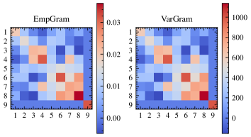
Figure 1: Mapping of the Empirical (left) and proposed (right) observability Gramians. The square colors indicate the strength and direction of the relations between the variables. Color contrast represents strength while the color itself represents the direction of interrelations.

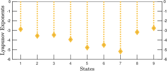
Figure 2: Lyapunov exponents computed for the $\mathrm{H}_{2}\mathrm{O}_{2}$ reaction network.

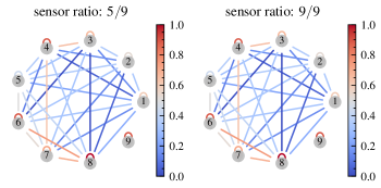
Figure 3: Normalized observability relation between state variables based on $(5/9)$ sensor node ratio (left) and full node sensor ratio (right) for the sensed nodes within the nonlinear system. For left figure, sensed nodes are optimally chosen as $\{1,\;2\;,4\;,6\;,9\}$.

The greedy algorithm [11, Algorithm 1] is employed to solve the SNS problem $\mathbf{P1}$ with (27) as the submodular objective function. We solve for optimal sensor selection with $r=5$ using the $\mathrm{log}$-$\mathrm{det}$ measure. The optimally selected subset of the sensor nodes is $\{1\;,2\;,4\;,6\;,9\}$ for $\mathrm{H}_{2}\mathrm{O}_{2}$ network. Fig. 3 depicts the normalized internal state relations for sensor ratio $5/9$ and that of a full sensor selection ratio. Notice that node $9$ has a self-loop thereby indicating that it is a non-interacting chemical species. This means that node $9$ is only observable when the same node is selected. The strength of the state relations and interactions are similar for both sensor fractions thereby indicating the optimality of the chosen sensor subset with $r=5$. Such equivalence validates that the sensor nodes selected using the proposed submodular set optimization framework are optimal. This is also evident in Fig. 4 where it is shown that the estimation error approaches zero for the optimal solution when considering $r=5$ for the $\mathrm{H}_{2}\mathrm{O}_{2}$ network. Note that the estimation error is related to the observability of the system.

The estimation error is computed using the following formula $e=\left\|\bm{x}-\hat{\bm{x}}\right\|_{2}/\left\|\bm{x}\right\|_{2}$, where $\bm{x}$ is the true state and $\hat{\bm{x}}$ is the estimate obtained by solving a general nonlinear least squares state estimation problem for the observation horizon $\mathrm{N}$. For the $\mathrm{H}_{2}\mathrm{O}_{2}$ and $\mathrm{GRI}30$ networks, we solve $\mathbf{P1}$ for different sensor ratios and compute the estimation error. Notice that, for $\mathrm{GRI}30$ network the estimation error decreases but does not reach an optimal error value due to a large number of non-interacting species. This indicated that additional sensors are required for better state estimation. We also note that utilizing a greedy approach yields an efficient and scalable solution to the observability-based SNS problem in nonlinear systems as compared with methods that rely on empirical data simulations—as with Empr-Gram framework. Solving $\mathbf{P1}$ for the $\mathrm{H}_{2}\mathrm{O}_{2}$ under sensor ratio $5/9$ requires $0.414\;\mathrm{s}$. The computational effort increases to about $24.797\;\mathrm{s}$ for $\mathrm{GRI}30$ network when considering an equivalent sensor ratio. This shows that the proposed SNS framework is scalable for larger nonlinear networks. For brevity, we do not introduce or solve the SNS framework based on the Empr-Gram, and therefore, we do not provide a comparison. However, based on the computational time provided in Tab. 1, it is inferred that solving $\mathbf{P1}$ requires significantly more effort. The computational efficiency along with the optimality results provided by Fig. 3 and Fig. 4 validate the modularity of the proposed Var-Gram and its submodular observability measure $\mathrm{log}$-$\mathrm{det}$ for SNS in nonlinear systems and thereby answers question $\mathrm{Q}3$. On this note, we conclude this section.

7 Summary and Future Directions

This technical note introduces a new observability Gramian for nonlinear dynamical systems. The formulated nonlinear observability Gramian is based on a discrete-time variational nonlinear system representation. The Gramian is proved to be equivalent to the Empr-Gram and that it reduces to the observability Gramian when considering a linear system. Connections between the introduced observability notion and Lyapunov exponents are illustrated. We derive a spectral observability limitation result that arises from the proposed Var-Gram. To further showcase the validity of this approach, we demonstrate its applicability under the context of observability-based sensor node selection. The proposed observability notion, in its current form, is not devoid of limitations; further research is worthy of investigation. The method is developed for general nonlinear systems without considering control input. Nonlinear networks under control input will be considered in our future work. Furthermore, extension of this method for stochastic nonlinear systems is important; such extension is demonstrated for the Empr-Gram [44].

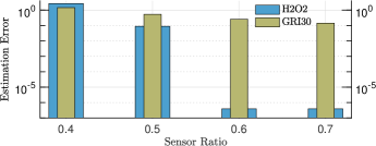
Figure 4: State estimation error based on the optimal SNS. The performance of the state estimation depends on the degree of system observability.

References

- [1] Y. Kawano and T. Ohtsuka, “Observability at an initial state for polynomial systems,” Automatica, vol. 49, no. 5, pp. 1126–1136, 2013.
- [2] R. E. Kalman, “Mathematical Description of Linear Dynamical Systems,” Journal of the Society for Industrial and Applied Mathematics Series A Control, vol. 1, no. 2, pp. 85–239, 1963.
- [3] R. Hermann and A. J. Krener, “Nonlinear Controllability and Observability,” IEEE Transactions on Automatic Control, vol. 22, no. 5, pp. 728–740, 1977.
- [4] A. J. Whalen, S. N. Brennan, T. D. Sauer, and S. J. Schiff, “Observability and controllability of nonlinear networks: The role of symmetry,” Physical Review X, vol. 5, no. 1, pp. 1–40, 2015.
- [5] A. J. Krener and K. Ide, “Measures of unobservability,” Proceedings of the IEEE Conference on Decision and Control, pp. 6401–6406, 2009.
- [6] B. C. Moore, “Principal Component Analysis in Linear Systems: Controllability, Observability, and Model Reduction,” IEEE Transactions on Automatic Control, vol. 26, no. 1, pp. 17–32, 1981.
- [7] S. Lall, J. E. Marsden, and S. Glavaški, “Empirical model reduction of controlled nonlinear systems,” IFAC Proceedings Volumes, vol. 32, no. 2, pp. 2598–2603, 1999.
- [8] ——, “A subspace approach to balanced truncation for model reduction of nonlinear control systems,” International Journal of Robust and Nonlinear Control, vol. 12, no. 6, pp. 519–535, 2002.
- [9] L. Kunwoo, Y. Umezu, K. Konno, and K. Kashima, “Observability Gramian for Bayesian Inference in Nonlinear Systems with Its Industrial Application,” IEEE Control Systems Letters, vol. 7, pp. 871–876, 2023.
- [10] A. Haber, F. Molnar, and A. E. Motter, “State Observation and Sensor Selection for Nonlinear Networks,” IEEE Transactions on Control of Network Systems, vol. 5, no. 2, pp. 694–708, 2018.
- [11] M. H. Kazma, S. A. Nugroho, A. Haber, and A. F. Taha, “State-Robust Observability Measures for Sensor Selection in Nonlinear Dynamic Systems,” 2023 62nd IEEE Conference on Decision and Control (CDC), no. Cdc, pp. 8418–8426, 2023. [Online]. Available: http://arxiv.org/abs/2307.07074
- [12] Y. Y. Liu and A. L. Barabási, “Control principles of complex systems,” Reviews of Modern Physics, vol. 88, no. 3, pp. 1–58, 2016.
- [13] Aleksandr Mikhailovich Lyapunov, “General Problem Of the Stability of Motion,” 1892.
- [14] A. Czornik, A. Konyukh, I. Konyukh, M. Niezabitowski, and J. Orwat, “On Lyapunov and Upper Bohl Exponents of Diagonal Discrete Linear Time-Varying Systems,” IEEE Transactions on Automatic Control, vol. 64, no. 12, pp. 5171–5174, 2019.
- [15] K. Krishna, S. L. Brunton, and Z. Song, “Finite Time Lyapunov Exponent Analysis of Model Predictive Control and Reinforcement Learning,” arXiv, pp. 1–22, 2023.
- [16] L. Barreira, Lyapunov Exponents, 1998.
- [17] J. Cortés, A. Van Der Schaft, and P. E. Crouch, “Characterization of gradient control systems,” SIAM Journal on Control and Optimization, vol. 44, no. 4, pp. 1192–1214, 2005.
- [18] Y. Kawano and J. M. Scherpen, “Empirical differential Gramians for nonlinear model reduction,” Automatica, vol. 127, p. 109534, 2021.
- [19] M. Balcerzak, A. Dabrowski, B. Blazejczyk-Okolewska, and A. Stefanski, “Determining Lyapunov exponents of non-smooth systems: Perturbation vectors approach,” Mechanical Systems and Signal Processing, vol. 141, p. 106734, 2020.
- [20] L. S. Young, “Mathematical theory of Lyapunov exponents,” Journal of Physics A: Mathematical and Theoretical, vol. 46, no. 25, 2013.
- [21] A. Iserles, A First Course in the numerical analysis of differential equations, 2nd ed. Cambridge University Press, 2009.
- [22] K. E. Atkinson, W. Han, and D. Stewart, “Numerical Solution of Ordinary Differential Equations,” Numerical Solution of Ordinary Differential Equations, pp. 1–252, 2011.
- [23] S. C. Shadden, F. Lekien, and J. E. Marsden, “Definition and properties of Lagrangian coherent structures from finite-time Lyapunov exponents in two-dimensional aperiodic flows,” Physica D: Nonlinear Phenomena, vol. 212, no. 3-4, pp. 271–304, 2005.
- [24] D. K. Arrowsmith and C. M. Place, Dynamical systems: differential equations, maps and chaotic behaviour, first edit ed. Chapman and Hall, 1994.
- [25] S. Hanba, “Existence of an observation window of finite width for continuous-time autonomous nonlinear systems,” Automatica, vol. 75, pp. 154–157, 2017.
- [26] ——, “On the “Uniform” Observability of Discrete-Time Nonlinear Systems,” IEEE Transactions on Automatic Control, vol. 54, no. 8, pp. 1925–1928, 2009.
- [27] S. Smale, “Mathematical problems for the next century,” The Mathematical intelligencer, vol. 20, no. 2, pp. 7–15, 1998.
- [28] N. D. Powel and K. A. Morgansen, “Empirical observability Gramian rank condition for weak observability of nonlinear systems with control,” Proceedings of the IEEE Conference on Decision and Control, vol. 54th IEEE, no. Cdc, pp. 6342–6348, 2015.
- [29] A. Mesbahi, J. Bu, and M. Mesbahi, “Nonlinear observability via Koopman Analysis: Characterizing the role of symmetry,” Automatica, vol. 124, p. 109353, 2021.
- [30] D. Martini, D. Angeli, G. Innocenti, and A. Tesi, “Ruling Out Positive Lyapunov Exponents by Using the Jacobian’s Second Additive Compound Matrix,” IEEE Control Systems Letters, vol. 6, pp. 2924–2928, 2022.
- [31] S. G. Krantz and H. R. Parks, The Implicit Function Theorem: History, Theory, and Applications. Springer New York, 2013.
- [32] T. H. Summers, F. L. Cortesi, and J. Lygeros, “On Submodularity and Controllability in Complex Dynamical Networks,” IEEE Transactions on Control of Network Systems, vol. 3, no. 1, pp. 91–101, mar 2016.
- [33] A. Pikovsky and A. Politi, Lyapunov Exponents: A Tool to Explore Complex Dynamics, 2017, vol. 70, no. 3.
- [34] P. J. Nolan, M. Serra, and S. D. Ross, “Finite-time Lyapunov exponents in the instantaneous limit and material transport,” Nonlinear Dynamics, vol. 100, no. 4, pp. 3825–3852, 2020.
- [35] M. Tranninger, R. Seeber, S. Zhuk, M. Steinberger, and M. Horn, “Detectability Analysis and Observer Design for Linear Time Varying Systems,” IEEE Control Systems Letters, vol. 4, no. 2, pp. 331–336, 2020.
- [36] J. Frank and S. Zhuk, “A detectability criterion and data assimilation for nonlinear differential equations,” Nonlinearity, vol. 31, no. 11, pp. 5235–5257, 2018.
- [37] N. Barabanov, “Lyapunov exponent and joint spectral radius: Some known and new results,” Proceedings of the 44th IEEE Conference on Decision and Control, and the European Control Conference, CDC-ECC ’05, vol. 2005, no. 3, pp. 2332–2337, 2005.
- [38] G. Rota and W. Gilbert Strang, “A note on the joint spectral radius,” Indagationes Mathematicae (Proceedings), vol. 63, no. 638, pp. 379–381, 1960.
- [39] S. Joshi and S. Boyd, “Sensor selection via convex optimization,” IEEE Transactions on Signal Processing, vol. 57, no. 2, pp. 451–462, 2009.
- [40] K. Manohar, J. N. Kutz, and S. L. Brunton, “Optimal Sensor and Actuator Selection Using Balanced Model Reduction,” IEEE Transactions on Automatic Control, vol. 67, no. 4, pp. 2108–2115, 2022.
- [41] L. Lovász, Submodular functions and convexity. Berlin, Heidelberg: Springer Berlin Heidelberg, 1983, pp. 235–257.
- [42] L. Zhou and P. Tokekar, “Sensor Assignment Algorithms to Improve Observability while Tracking Targets,” IEEE Transactions on Robotics, vol. 35, no. 5, pp. 1206–1219, 2019.
- [43] N. N. Smirnov and V. F. Nikitin, “Modeling and simulation of hydrogen combustion in engines,” International Journal of Hydrogen Energy, vol. 39, no. 2, pp. 1122–1136, 2014.
- [44] N. Powel and K. A. Morgansen, “Empirical Observability Gramian for Stochastic Observability of Nonlinear Systems,” arXiv, jun 2020.