Engineering and Revealing Dirac Strings in Spinor Condensates

Abstract

Artificial monopoles have been engineered in various systems, yet there has been no systematic study on the singular vector potentials associated with the monopole field. We show that the Dirac string, the line singularity of the vector potential, can be engineered, manipulated, and made manifest in a spinor atomic condensate. We elucidate the connection among spin, orbital degrees of freedom, and the artificial gauge, and reveal that there exists a mapping between the vortex filament and the Dirac string. We also devise a proposal where preparing initial spin states with relevant symmetries can result in different vortex patterns, revealing an underlying correspondence between the internal spin states and the spherical vortex structures. Such a mapping also leads to a new way of constructing monopole harmonics. Our observation provides significant insights in quantum matter possessing internal symmetries in curved spaces.

Introduction —

Despite of the lack of unambiguous experimental evidence for their existence, magnetic monopoles have a central place in our understanding of quantum matter and modern cosmology [1, 2, 3, 4]. Remarkably, recent theories and experiments have provided ample evidences for the emergence of artificial monopoles in various physical systems [5, 6, 7, 8, 9, 10, 9, 11, 12, 13, 14, 15, 16]. It is well known that the vector potential associated with the monopole field contains line singularities (known as Dirac strings) that terminate at the monopole, even though the monopole magnetic field itself is smooth everywhere (except at the position of the monopole) [17]. This does not pose any problem as the vector potential, unlike the field, is not “real” in the sense that it cannot be directly measured. This is also reflected in the fact that the positions of these Dirac strings are gauge dependent.

This conventional wisdom, however, is not necessarily true in systems with artificial gauge fields. In such systems, one often directly realizes and controls the artificial gauge potential, rather than the associated ‘magnetic’ field, rendering the former directly measurable. Indeed, the physical effects of artificial gauge potentials on time-of-flight images of cold atoms have been reported in several experiments  [18, 19, 20, 21, 22].

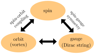
Figure 1: Conceptual plot showing the connection among spin, orbit degrees of freedom, and the artificial gauge field.

One widely used platform to realize artificial gauge field is spinor Bose-Einstein Condensates (BECs). When the atomic spin  adiabatically follows an external magnetic field, the system accumulates a geometric phase  [24], which induces an artificial gauge potential governing the spatial wave function; a manifestation of the spin-orbit coupling. If the atoms occupy a spatial region that contains a degenerate point with vanishing magnetic field, the artificial gauge potential can develop a line singularity, which can be regarded as an analog of the Dirac string and a consequence of the local spin-gauge symmetry [9, 25]. The purpose of this work is to elucidate the relationship among spin, orbit and the artificial gauge field. As conceptually represented in Fig. 1, through the spin-orbit coupling and the spin-gauge symmetry, there exists a mapping between the vortex filament and the Dirac string. This directly leads to a novel adiabatic scheme for preparing vortex configurations on a sphere where some initial spin state is prepared for the spinor condensate, and then the artificial magnetic field strength is turned on adiabatically. As a result of conservation of the total angular momentum, some of the initial spin angular momentum is transferred to the orbital degrees of freedom, resulting in the formation of vortices. Preparing different initial spin states can therefore result in different vortex patterns. From the point of view of the artificial gauge field, this amounts to different gauge choices that lead to different Dirac strings.

Spin, vortex, and Dirac strings —

Let us consider a spin-$F$ atom of mass $M$ confined in an isotropic harmonic trapping potential with frequency $\omega$, subjected to a hedgehog magnetic field ${\bf B}({\bm{r}})\propto{\bm{r}}$. The realization of the hedgehog field has been proposed in our earlier work [26]. Working in units where $\hbar=M=\omega=1$, the single-particle Hamiltonian of the system reads

$$H_{0}(\bm{r})=-\frac{\nabla^{2}}{2}+\frac{r^{2}}{2}-\alpha r\hat{\bm{r}}\cdot\mathbf{F}\,.$$ (1)

Here $\alpha$ characterizes the strength of the hedgehog field, which we assume can be dialled from zero to large values. In the limit of large field strength $\alpha r$, the lowest spin state follows the local magnetic field and satisfies $(\hat{\bm{r}}\cdot{\bf F})|F_{\hat{\bm{r}}}\rangle=F|F_{\hat{\bm{r}}}\rangle$, where $|F_{\hat{\bm{r}}}\rangle$ can be obtained from $|F_{\hat{\bm{z}}}\rangle$ (the spin state polarized along the $z$-axis) via rotations: $\left|F_{\hat{\bm{r}}}\right\rangle=e^{-i\varphi F_{z}}e^{-i\theta F_{y}}\left|F_{\hat{\bm{z}}}\right\rangle$. Here $\theta$ and $\varphi$ are the polar and azimuthal angles respectively. The total wave function, $\Psi({\bm{r}})$, can be written as $\Psi({\bm{r}})=\psi({\bm{r}})|F_{\hat{\bm{r}}}\rangle$, with the effective Hamiltonian of the scalar wave function $\psi({\bm{r}})$ being:

$$H_{\rm eff}+\frac{\alpha^{2}F^{2}}{2}=\frac{1}{2}(-i\nabla+{\bf A})^{2}+\frac{1}{2}(r-\alpha F)^{2}+\frac{F}{2r^{2}}\,.$$ (2)

Here the effective vector potential ${\bf A}=i\langle F_{\hat{\bm{r}}}|\nabla F_{\hat{\bm{r}}}\rangle=\hat{e}_{\varphi}\,F\cos\theta/(r\sin\theta)$ reflects an ‘magnetic’ monopole (of magnetic charge $F$) at the origin. Furthermore, the last term in Eq. (2) dictates that this monopole is also ‘electrically polarized’, with an electric dipole moment $F/2$. The vector potential ${\bf A}$ is singular for $\theta=0$ and $\pi$, which corresponds to two antipodal Dirac strings. It can be seen that the effective system realises a Haldane’s sphere [27]: atoms of unit ‘electric charge’, are confined within a thin spherical shell (of width $\sim\sqrt{M\omega}$) centered at $r_{0}\approx\alpha F$, in the presence of an ‘electrically polarized magnetic monopole’ at the origin.

If we rewrite the scalar function above as $\psi({\bm{r}})=\sqrt{n({\bm{r}})}e^{i\phi({\bf r})}$, where $n({\bm{r}})$ represents the local atomic number density, then the total wavefunction can be written as $\Psi({\bm{r}})=\sqrt{n({\bm{r}})}|\tilde{F}_{\hat{\bm{r}}}\rangle$, where $|\tilde{F}_{\hat{\bm{r}}}\rangle=e^{i\phi({\bf r})}|{F}_{\hat{\bm{r}}}\rangle$. In other words, we have absorbed the phase factor of the scalar function into a redefinition of the radial spin state. The corresponding vector potential associated with $|\tilde{F}_{\hat{\bm{r}}}\rangle$ is given by $\tilde{\bf A}=i\langle\tilde{F}_{\hat{\bm{r}}}|\nabla\tilde{F}_{\hat{\bm{r}}}\rangle={\bf A}+\nabla\phi$, which is related to ${\bf A}$ by a gauge transformation. This is just a manifestation of the spin-gauge symmetry in spinor gases [25]. On the other hand the velocity field associated with the total wavefunction $\Psi({\bm{r}})$ is given by $\bm{v}^{\text{mass}}=-\nabla\phi-{\bf A}=-\tilde{\bf A}$, which allows us to clearly see the connection between vortices (line singularities of $\bm{v}^{{\rm mass}}$) and line singularities of $\tilde{\bf A}$. As we will show in the following, by preparing different initial spin configurations in the absence of the monopole field followed by its adiabatic turn on, we may result in final states with different phase structure $\phi({\bf r})$, and hence different vortex or Dirac string orientations. In a sense, changing the initial spin configuration amounts to choosing a different gauge for the vector potential $\tilde{\bf A}$.

Engineering Dirac Strings —

To substantiate the argument we laid out above, here we provide a more quantitative description.

Single-particle spectrum

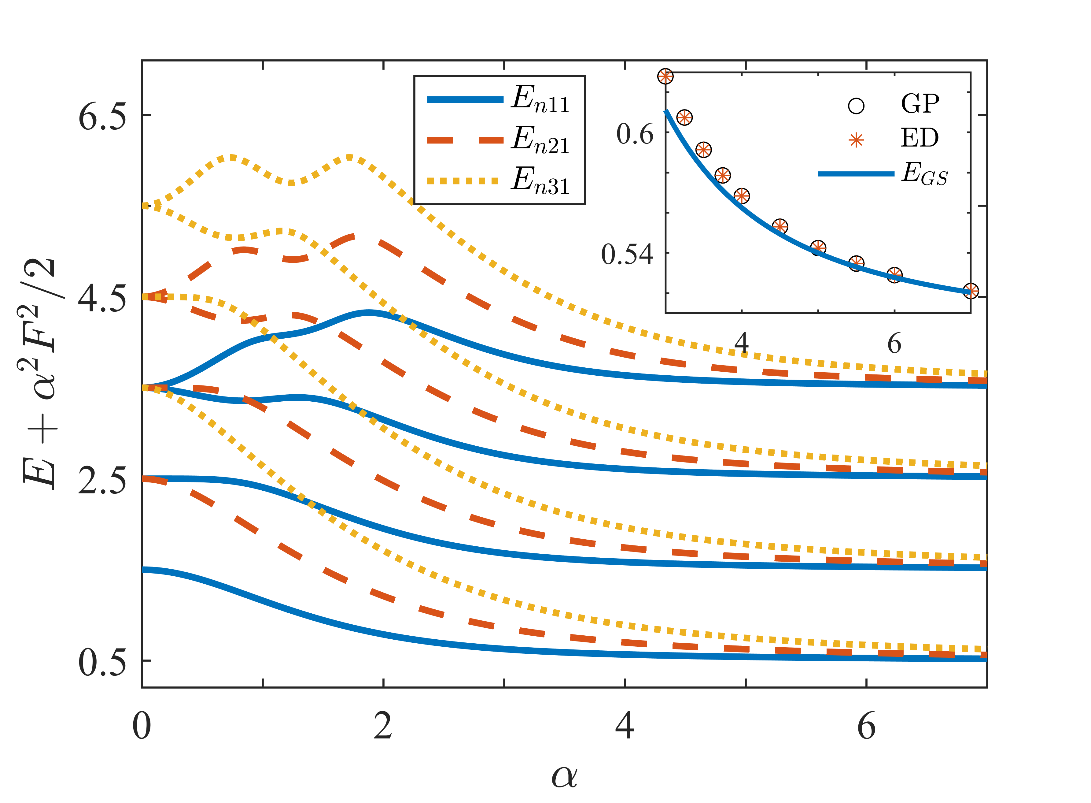
Figure 2: Numerical calculation of the single-particle energy spectrum $E_{njF}$ (shifted by $\alpha^{2}F^{2}/2$) as a function of $\alpha$, for the $F=1$ case. As $\alpha$ increases, levels of $(j=1,n-1)$ (solid blue), $(j=2,n)$ (dashed red), and $(j=3,n+1)$ (dotted yellow) approach each other, while a crossover from the 3D isotropic oscillator to the 1D LL occurs. The inset shows the lowest energy $E_{011}$ in the adiabatic regime, which is obtained from GP equations (circle), ED (star) and the analysis in Eq. (5) (solid).

Let us first consider the single-particle spectrum for the Hamiltonian (1). It can be seen that while for $\alpha=0$ both ${\bf L}$ and ${\bf F}$ are conserved, for $\alpha\neq 0$ only the total angular momentum (TAM) ${\bf J}={\bf L}+{\bf F}$ is conserved. This means that the energy eigenstates are also eigenstates of $\{{\bf J}^{2},J_{z}\}$. These are the well-known spinor harmonics $|\chi_{jm}^{\ell F}\rangle=\sum^{F}_{m_{F}=-F}c_{jm}^{\ell m_{F}}Y^{\ell}_{m-m_{F}}(\hat{\bm{r}})|{m_{F}}_{\hat{\bm{z}}}\rangle$ [28], where, $c$’s are the Clebsch-Gordan coefficients, $Y$’s are the usual spherical harmonics, and $|{m_{F}}_{\hat{\bm{z}}}\rangle$ are the spin multiplicity states (in the $z$ basis). Furthermore, while ${\bf F}^{2}$ is conserved, ${\bf L}^{2}$ is not. Summing over the $\ell$ quantum number then, the eigenstates take the form

$$\Psi_{njmF}({\bm{r}})=\sum^{j+F}_{\ell=|j-F|}f_{njF}^{\ell}(r)|\chi_{jm}^{\ell F}(\hat{\bm{r}})\rangle\,.$$ (3)

The Hamiltonian (1) can then be diagonalized by decomposing the Zeeman term as $\bm{r}\cdot\mathbf{F}=(A+A^{\dagger})/\sqrt{2}$ and using the group SU(1,1)$\times$SU(2). Here the operators $A^{\dagger}\equiv\mathbf{F}\cdot\bm{a}^{\dagger}$ and $A$ are rank-0 tensors under rotations generated by ${\bf J}$, and $a_{i}^{\dagger}$ ($a_{i}$) are bosonic creation (annihilation) operators [29]. In Fig. 2 we provide different energy curves as a function of $\alpha$, for different $n$ and $j$ values.

From the point of view of the adiabatic flow of local spin, the radial part of the scalar function $\psi$ corresponds to a $1$D harmonic oscillator centered at radius $r_{0}$ (c.f. Eq. (2)), while the angular structure is dictated by the Hamiltonian $H_{\Omega}=[({\bm{r}}\times({\bm{p}}+{\bf A}))^{2}+F]/(2\alpha^{2}F^{2})$. That is, the function $\psi$ takes the form $\psi({\bm{r}})\approx r^{-1}h_{n}(r-r_{0})\,g^{m}_{F,j}(\theta,\varphi)$, where $h_{n}$ are the usual harmonic oscillator states and $g^{m}_{F,j}$ are the eigenstates of the angular Hamiltonian $H_{\Omega}$. Then with the ansatz $f^{\ell}_{njF}(r)\equiv r^{-1}h_{n}(r-r_{0})\,\beta^{\ell}_{F,j}$ in Eq. (3), the $\beta$ coefficients must be such that the following holds

$$\sum^{j+F}_{\ell=|j-F|}\beta^{\ell}_{F,j}|\chi^{\ell F}_{jm}\rangle\approx g^{m}_{F,j}(\theta,\varphi)|F_{\hat{\bm{r}}}\rangle\,.$$ (4)

This is the adiabatic flow condition, and can be used to determine the $\beta$ coefficients and the functions $g$. We note that only for $j\geq F$, can we have the above relation satisfied. Using Eq. (4), we can further determine the energy spectrum in the adiabatic regime:

$$E_{njF}+\frac{\alpha^{2}F^{2}}{2} \approx n+\frac{1}{2}+\frac{(j-F+1)(j+F)}{2\alpha^{2}F^{2}}\,.$$ (5)

The last term is just the spherical Landau levels (LLs) [27], plus a shift $F/(2\alpha^{2}F^{2})$ owing to the ‘electric dipole moment’. Note that all the different $j$ levels approach one another as $\alpha$ increases, because the energy of different states gets increasingly dominated by the Zeeman term.

As an explicit example, consider the spin-$1$ case. For the lowest $j=1$ level, we get $\beta^{\ell}_{1,1}=\{\sqrt{2},\sqrt{3},1\}/\sqrt{6}$ for $\ell=\{0,1,2\}$, and the following three degenerate states

$$\Bigl{\{}\Psi_{n1-11},\,\Psi_{n101},\,\Psi_{n111}\Bigr{\}}\approx\frac{1}{2}\sqrt{\frac{3}{\pi}}\,\frac{1}{r}h_{n}(r-\alpha)\,\times$$

$$\quad\Biggl{\{}\sin^{2}\left(\frac{\theta}{2}\right)e^{-i\varphi},\,\frac{\sin\theta}{\sqrt{2}},\,\cos^{2}\left(\frac{\theta}{2}\right)e^{i\varphi}\Biggr{\}}\left|{F}_{\hat{\bm{r}}}\right\rangle\,.$$ (6)

The inset in Fig. 2 compares the energy with the the Gross-Pitaevskii (GP) equation, and exact diagonalization (ED). It is evident that the adiabatic flow condition holds well within $\sim 0.1\%$ for $\alpha\gtrsim 4$.

In general, it can be seen that the functions $g^{m}_{F,j}(\theta,\varphi)$ are exactly the eigenstates $\mathcal{Y}_{q,j}^{m}(\theta,\varphi)$ of the $j{\rm th}$ spherical LL with magnetic charge $q=F$, otherwise known as the monopole harmonics. This reveals an alternative approach to constructing higher spherical LLs.

Creating vortices from different spin states:

Conservation of ${\bf J}$ can be exploited to create vortex patterns/Dirac strings, as follows. Starting at $\alpha=0$, we can prepare the system in its ground state, carrying zero orbital angular momentum (OAM) $\langle{\bf L}\rangle_{\rm ini}=0$ and any desired spin configuration $|\zeta^{x}\rangle$ carrying spin angular momentum (SAM) $\langle{\bf F}\rangle_{\rm ini}$. Then $\alpha$ is increased adiabatically, and in the process some of the SAM gets transferred to the OAM while keeping the total $\langle{\bf J}\rangle$ fixed. At sufficiently large $\alpha$ owing to adiabatic spin flow, we converge to a vortex pattern in the final state carrying final OAM $\langle{\bf L}\rangle_{\rm fin}=\langle{\bf F}\rangle_{\rm ini}/(1+F)$ and SAM $\langle{\bf F}\rangle_{f}=F\langle{\bf F}\rangle_{\rm ini}/(1+F)$ [29].

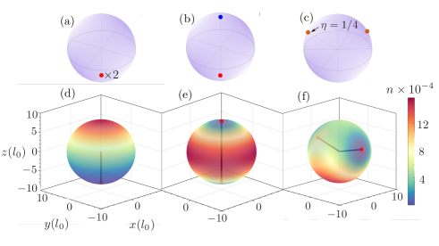
Figure 3: Upper panel: Majorana representations of spin-1 (a) ferromagnetic state $\zeta^{F}=(1,0,0)^{T}$, (b) polar state $\zeta^{P}=(0,1,0)^{T}$, and (c) mixed state $\zeta^{\eta}=(\sqrt{\eta},0,\sqrt{1-\eta})^{T}$ with $\eta=1/4$ on the Bloch sphere. Lower panel: corresponding density profiles on the sphere of radius $r_{0}=\alpha=8$. Black lines represent the vortex lines, with the intersection points with atomic cloud at $r_{0}$ being Majorana stars.

We can also predict the orientation of these Dirac strings (which are lines of singularities) by considering the geometric/Bloch sphere representation for spin-$F$. We note that at points where the strings/vortices intersect the sphere, the ‘wavefunction’ must vanish. Then, owing to the transfer of initial SAM to final TAM during the adiabatic spin flow, these intersection points should be where the initial spin configuration $|\zeta^{x}\rangle$ was orthogonal to the final spin configuration $|F_{\hat{\bm{r}}}\rangle$. With $|\zeta^{x}\rangle=\sum_{m_{F}=-F}^{F}\zeta^{x}_{m_{F}}|m_{F\,{\hat{\bm{z}}}}\rangle$ and $|F_{\hat{\bm{r}}}\rangle=e^{-i\varphi F_{z}}e^{-i\theta F_{y}}\left|F_{\hat{\bm{z}}}\right\rangle$, this means those points $(\theta,\varphi)$ on the sphere where $\langle\zeta^{x}|F_{\hat{\bm{r}}}\rangle=0$:

$$\sum^{2F}_{k=0}e^{-ik\varphi}\,\zeta^{x}_{F-k}\sqrt{\begin{pmatrix}2F\\ k\end{pmatrix}}\cos^{2F}\left(\frac{\theta}{2}\right)\,\tan^{k}\left(\frac{\theta}{2}\right)=0\,.$$ (7)

Note that these points are nothing but the so called Majorana stars, and our engineering of the Dirac strings reveals the connection between spin and real space. This connection is embodied in the $\mathrm{SO(3)}$ symmetry in both the spinor Boson gas and the simulated monopole system. More explicitly, the symmetries of $\left|\zeta^{x}\right\rangle$ correspond to the operations under which the set of vortex locations $\left\{(\theta_{i},\varphi_{i})\right\}$ on the Haldane sphere are invariants.

As explicit examples, consider the following ferromagnetic, polar and mixed states to begin with: $|\zeta^{F}\rangle=(1,0,0)^{T}$, $|\zeta^{P}\rangle=(0,1,0)^{T}$, and $|\zeta^{\eta}\rangle=(\sqrt{\eta},0,\sqrt{1-\eta})^{T}$. Based on our discussion above and Eq. (7), each would correspond to two Dirac strings/vortices at large $\alpha$, originating from the origin. Their locations are calculated to be $\theta=\pi,\pi$ for ferromagnetic, $\theta=0,\pi$ for polar, and $(\theta,\varphi)=(2\arctan[\eta/(1-\eta)]^{1/4},\pi\pm\pi/2)$ for the mixed state. The full final states, written in terms of the lowest LL (LLL) wavefunction in (Single-particle spectrum) are: $\Psi^{F}=\Psi_{0111}$, $\Psi^{P}=\Psi_{0101}$, and $\Psi^{\eta}=\sqrt{\eta}\,\Psi_{0111}+\sqrt{1-\eta}\,\Psi_{01-11}$. In the lower panel of Fig. 3, we show these states obtained using the normalized gradient flow method of [30]. The upper panel displays the Majorana representations of $\zeta^{F}$, $\zeta^{P}$ and $\zeta^{\eta}$, respectively, where the highlighted points on the sphere correspond to (7).

In Fig. 4, we show the real time implementation of our idea, for the mixed state $|\zeta^{\eta=1/4}\rangle$, using the integrator i-SPin 2 [31]. Starting with the 3D harmonic oscillator ground state dressed with the spin texture $|\zeta^{\eta=1/4}\rangle$, we adiabatically increase $\alpha$ from $0$ to $6$ . As $\alpha$ increases, the initial mass density at the origin is pushed outwards, with the spin density aligning radially outwards. At large enough $\alpha$, two vortices intersecting the atomic cloud at $(\theta,\varphi)=(2\arctan[1/3]^{1/4},\pi\pm\pi/2)$, become apparent. One can also get these locations by means of the vortex Dirac string connection: Rewriting the state as $\Psi^{\eta}=|\psi^{\eta}||F_{\hat{\bm{r}}}\rangle$ where $|\tilde{F}_{\hat{\bm{r}}}\rangle=\exp(i\,{\rm arg}\,\psi^{\eta})|F_{\hat{\bm{r}}}\rangle$, it can be shown that the effective gauge potential $\tilde{\bf A}=i\langle\tilde{F}_{\hat{\bm{r}}}|\nabla\tilde{F}_{\hat{\bm{r}}}\rangle$ contains two singularities located at $(2\tan^{-1}[1/3]^{1/4},\pi\pm\pi/2)$ when $\eta=1/4$.

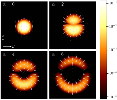
Figure 4: Evolution of the mixed state $\zeta^{\eta=1/4}$ when the field strength $\alpha$ is increased adiabatically from 0 to 6. The density profile (background color) and local spin expectation vector $\langle{\bf F}(\mathbf{r})\rangle$ (arrows) in the $x=0$ plane are plotted at four different times with the instataneous values of $\alpha$ indicated in the plots. For each plot, the length of the box along each direction is 25, and the calculation is done with a grid size $N^{3}=71^{3}$.

To summarize, we have established a one-to-one mapping between the spinor state and the vortex state on a sphere. The adiabatic turning on the external field will preserve and transfer the remaining symmetry from the spin space to the real space. In other words, $|\zeta\rangle$ and $\tilde{\psi}$ with the same angular momentum are classified into the same isotropy group. This, ultimately, arises from the isotropic spin-orbit coupling in the system.

Effects of Interaction and Experimental Feasibility —

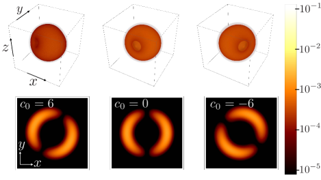
Figure 5: Snapshots of the mixed state atomic cloud for $\eta=1/4$ at $\alpha=6$, for the three cases of attractive interaction ($c_{0}=-6$ and $c_{2}=-0.1$, left column), no interaction ($c_{0}=c_{2}=0$, middle column), and repulsive interaction ($c_{0}=6$ and $c_{2}=0.1$, right column), respectively. Other parameters are the same as in Fig. 4. The upper panel shows a 3D view, whereas the bottom panel shows the slice in the plane where the vortices intersect the atomic cloud (at polar angle $\theta=2\tan^{-1}(1/3)^{1/4}\approx 74.46$ degrees). Our results also confirmed that for the values of $c_{2}$ used here, the effect of the spin-dependent interaction is negligible.

Now we briefly discuss the effects of the mean-field interaction, energy functional of which is $E_{\mathrm{int}}=c_{0}\int d^{3}\bm{r}~{}n^{2}(\bm{r})/2+c_{2}\int d^{3}\bm{r}~{}\bm{S}(\bm{r})\cdot\bm{S}(\bm{r})$, where $\bm{S}(\bm{r})$ is the local spin density, and the first and the second term in $E_{\mathrm{int}}$ corresponds to the spin-independent and -dependent interaction, respectively. Typically the two interaction strengths satisfy $|c_{0}|\gg|c_{2}|$. Figure 5 illustrates the final density profiles for the mixed state (with $\eta=1/4$), for attractive, non-interacting and repulsive interaction cases, when starting from the respective ground states in the absence of the spin-dependent interaction we ramp up $\alpha$ from $0$ to $6$. While some of the qualitative physics remains the same, there are some important distinctions worth pointing out: (1) Without interactions, it can be seen that all single-particle states $\mathcal{Y}^{m}_{F,F}$ (or linear combinations thereof), are left invariant under SO($2$)${}_{L_{z}+\phi}$ (here $\phi$ corresponds to gauge transformations). Including the interaction breaks this invariance and the states get rotated along the $z$ axis, as reflected by the rotation of vortex pairs. (2) In the final state, the angular momenta are not evenly distributed in the spin and the orbital sector. This is because the spin texture becomes more (an-)isotropic under the (attractive) repulsive interaction .

For $N=10^{4}$ ${}^{87}\mathrm{Rb}$ atoms in a trap with frequency $\omega=2\pi\times 100Hz$, and Zeeman field $B\bm{r}$ with strength $B=1.1\,G\,cm^{-1}$, the field strength $\alpha\simeq R=6.788$ reaches the regime where the adiabatic flow condition holds well. Also, the energy scale of the contact interaction $E_{c_{0}}\sim c_{0}/(32\pi^{2}\alpha^{2})$ is two order of magnitude smaller than the LL gap $\Delta E_{12}\sim 4/\alpha^{2}$. Therefore, the interaction is weak enough such that the analytical results presented for non-interacting system remain qualitatively correct.

Conclusions

The simulation of singular monopole potentials and the concomitant correspondence between the spin and the real space is a new feature of the spinor system under hedgehog magnetic field. The key ingredient is the rotational invariance of the Zeeman term ${\bm{r}}\cdot{\bf F}$. These will persist even when the $S_{2}$ manifold is deformed as long as $J_{z}$ remains conserved. Due to this rationale, we can investigate such features in other SO(3) systems, such as the isotropic spin-orbital-coupling term $\mathbf{p}\cdot\mathbf{F}$, where bent vortex lines in solitons have been discovered [34]. Remarkably, the correspondence presented in this paper allows us to reveal symmetries within the internal degrees of freedom, as manifesting in coordinate space.

In this work, we have found the spin real correspondence in the LLLs. Since stronger interactions may make the atoms occupy higher LLLs [35], correspondence in these states may be found. The investigation in Haldane’s spherical geometry was originally proposed for the study of the fractional quantum Hall effect. Thus fertile vortex configurations may enrich the exploration of many-body quantum matters in curved spatial geometry [36, 37, 38, 39, 40, 41, 42, 43].