Big data analytics to classify earthwork-related locations: A Chengdu study

Abstract

Air pollution has significantly intensified, leading to severe health consequences worldwide. Earthwork-related locations (ERLs) constitute significant sources of urban dust pollution. The effective management of ERLs has long posed challenges for governmental and environmental agencies, primarily due to their classification under different regulatory authorities, information barriers, delays in data updating, and a lack of dust suppression measures for various sources of dust pollution. To address these challenges, we classified urban dust pollution sources using dump truck trajectory, urban point of interest (POI), and land cover data. We compared several prediction models and investigated the relationship between features and dust pollution sources using real data. The results demonstrate that high-accuracy classification can be achieved with a limited number of features. This method was successfully implemented in the $AM\_system$ of Chengdu to provide decision support for urban pollution control.

I Introduction

Air pollution has increased dramatically in the last decade due to the development of the global economy [1]. According to the World Health Organization [2], nine in ten people worldwide breathe polluted air, underscoring the urgent need for urban air pollution control. Large-scale urban development is often closely related to the construction industry, which has become one of the main sources of dust pollution [3], especially during the construction phase [4], when the environmental impact is serious. Addressing the urgent challenge of overseeing the entire lifecycle of earthworks, from production through delivery to disposal, has become imperative. Furthermore, identifying earthwork-related locations (ERLs) and implementing focused regulatory measures is crucial for tackling this issue [5]. Timely discovery of these locations and the extraction of their characteristics can empower the relevant authorities to enact precise regulatory measures, ultimately enhancing the overall quality of the urban environment [5].

Researchers in earthwork management have mainly studied evaluation models for dust pollution [6, 7, 8, 9], dust emission patterns [10, 11, 12], and dump truck path planning [13, 14]. Most of these studies assume that the locations and categories of all the ERLs are known. However, approximately 60% of ERLs are unknown to local governments (Fig. 2), which poses a significant challenge for effective urban environmental management. In Chengdu City, over 14,000 dump trucks are equipped with GPS sensors, owing to the government’s increased attention and the ongoing development of big data technology. These dump trucks, which are specifically designed to transport construction waste and raw materials, play a crucial role in earthwork management. [15, 16] have successfully identified their work area, known as ERLs (Fig. 1) by analyzing the trajectory data from these GPS-equipped dump trucks, marking a notable advance in related research.

However, different categories of ERLs are usually overseen by different regulatory authorities, leading to challenges such as information barriers, slow data updating, and lack of dust suppression measures [5]. From discussions with relevant government staff and fieldworkers, we have learned that the current classification of ERLs relies primarily on manual checks and government-maintained ERL lists. However, manual checks are expensive and inefficient and government lists suffer from incomplete records and slow updates. Therefore, after identifying the ERL locations, classifying them becomes a crucial and challenging task. To the best of our knowledge, previous studies have not specifically addressed ERL classification; therefore, this current research fills this gap in the existing literature.

This study makes major contributions to several key areas.

• To the best of our knowledge, no previous study has attempted to classify ERLs. We introduce a nearly comprehensive set of features, including basic geographic, land cover, points of interest (POI), and dynamic features, for the description and classification of ERLs.

• We then employ four representative machine learning methods, namely, Logistic Regression (LR), Random Forest (RF), Gradient Boosted Decision Trees (GBDT), and Multilayer Perceptron (MLP). The results show that RF is the most effective.

• We employ the state-of-the-art SHAP method and feature distribution to extract the importance of features. Additionally, we provide a detailed description of the relationship between features and three categories of ERLs, revealing the characteristics of each category.

• The study’s results demonstrate that a RF model, considering only a select few factors ($distance\_center$, $stay\_time$, $all\_poi$, $grassland$, $business$, and $road\_fac$), can achieve a high-level performance.

The ERL classification algorithm was successfully deployed in the Alpha-MAPS Intelligent Atmospheric Monitoring and Control System ($AM\_System$) by the end of November 2023. In practical applications, the algorithm demonstrated favorable outcomes for $AM\_System$, achieving an ERL classification accuracy of 77.8%. With a gradual increase in the target labels, we anticipate that the algorithm’s performance will continue to improve. The application of the ERL classification algorithm enables relevant departments to have a more comprehensive understanding of ERLs, which provides decision support for environmental monitoring and governance in Chengdu and lays the foundation for related research.

This paper is organized as follows: Section II provides a comprehensive review of relevant research progress; Section III introduces concepts related to the problem and a nearly comprehensive set of features that could impact the categories of ERLs; Section IV describes the classification model, performance metrics, and feature importance identification employed in this study; subsequently, Sections V and VI present the computational results and the corresponding discussion; and finally, Section VII presents the system deployment and Section VIII presents the conclusions.

II Literature review

Large-scale urban development is often closely related to the construction industry and is one of the main sources of dust pollution [3]. According to our survey, research on earthwork pollution has raised extensive concerns regarding urban dust pollution management and intelligent transportation systems. Research on the management of urban dust pollution has primarily focused on dust pollution evaluation models [6, 7, 8, 9] and dust emission patterns [10, 11, 12]. Research on intelligent transportation systems has predominantly focused on traffic path planning [13, 14] for dump trucks. Although most of these studies examine dust pollution during transportation, the transportation process entails numerous uncertainties, and assessing its risks relies on understanding the sources of earth-moving pollution. Consequently, the identification and categorization of ERLs have become increasingly crucial for practical applications. Traditional methods rely primarily on manual processes, such as random sampling, which are labor-intensive and inefficient. Employing big data and artificial intelligence to facilitate the management of earthwork pollution is crucial.

The investigation of the sources of urban dust pollution also encompasses the field of big data mining. [17] describes big data technology as ”activities that can be performed on a large scale, impossible at smaller scales, to generate a novel form of value.” Numerous researchers have embraced three definitions of Big Data, namely volume, variety, and velocity, often referred to as the ‘three Vs’ [18]. Big Data analytics can reveal concealed patterns, unknown correlations, and other valuable insights [19]. [15] have identified stopping points from GPS track points of dump trucks using an adaptive spatio-temporal threshold method, while [16] have extracted long-term and regular earthwork point information using a grid clustering algorithm based on this data. By contrast, [20] have identified hot nodes in dump truck operations using Xgboost and DBSCAN. [19] have classified a specific operational pattern, namely illegal dumping. However, few studies have classified nodes related to earthwork. Nevertheless, note that [21] have identified and classified areas of hazardous material operations using trajectory data from hazardous material trucks. Our study aims to classify ERLs, thereby addressing a significant research gap in this field.

Big data and machine learning algorithms are closely intertwined. Machine learning algorithms are commonly classified into four categories: supervised, unsupervised, semi-supervised, and reinforcement learnings [22]. Supervised learning involves learning a function that maps inputs to outputs using input-output pairs of samples [23]. Supervised learning tasks typically encompass classification, which addresses discrete labeled data, and regression, which handles continuous labeled data. The data used for supervised learning may be structured or unstructured. Our research approach concentrates on multi-classification models utilizing structured data, employing commonly used algorithms, such as Naive Bayes, Linear Discriminant Analysis, Logistic Regression (LR), K-nearest neighbors (KNN), Support Vector Machine (SVM), Random Forest (RF), Adaptive Boosting (AdaBoost), and Multilayer Perceptron (MLP) [23, 24]. Model performance and interpretability are essential. However, machine learning models often lack interpretability, leading to the increased adoption of the SHAP method in research [25, 26]. The Shapley value, which is based on cooperative game theory, was originally proposed by Shapley in 1953 [27]. In 2017, [25] developed a Python package capable of computing SHAP values for various models, including Multilayer Perceptron (MLP) and Random Forest (RF), thereby simplifying the interpretation of machine learning models.

The literature review reveals significant interest among researchers regarding urban dust pollution. However, there have been no systematic investigations on the classification of ERLs. In this study, we utilize dump trucks, POI, and land cover data to employ various multi-classification machine learning methods to achieve highly accurate prediction results. In addition, we utilize the advanced SHAP method to elucidate the machine learning model. This study addresses the research gap in the classification of ERLs.

III Data

Chengdu is a megacity with an urban population exceeding 15 million; we selected its primary urban region as the study area. The study data are derived from research conducted by [15, 16]. As illustrated in Fig. 1, each ERL comprises multiple $200m\times 200m$ grids. The study period spans May 1, 2023, to June 31, 2023, encompassing a total of 61 days. Dump truck operations were categorized into daytime and nighttime shifts, with a defined 12-h duration for each shift. The day shift spans from 08:00:00 to 20:00:00, and the night shift spans from 20:00:00 to 08:00:00. As depicted in Fig. 2, approximately 600 and 250 ERLs were under construction during each day shift and night shift, respectively, with exceptions for extreme cases such as heavy pollution weather warnings. Additionally, we collected vehicle information, trajectory data, and stopping points for the dump trucks.

We classify ERLs into three categories: Earthwork_Related (ER), Material_Related (MR), and Parking & Maintenance (PM) (Table I). ER includes construction sites and dumping grounds, MR includes quarry and commercial concrete mixing stations, PM includes parking lots, automobile repair stations, and maintenance. The labeling data were sourced from a registry of ERLs provided by the relevant government departments, encompassing 2,403 ERLs of known categories. Approximately 60% of the ERLs have unknown category labels (Fig. 2). Our objective is to train and validate the model using the ERLs of known categories. There were 20,489 total samples from 122 shifts, comprised of 13,401 ERs, 1,559 MRs, and 5,529 PMs.

To accurately classify the categories of ERLs, we must thoroughly consider all features that may affect the classification accuracy. In this study, 58 numerical features are employed to establish a relatively comprehensive feature set of ERLs. The feature set encompasses four primary aspects: basic geographic features, land cover features, POI features, and dynamic features.

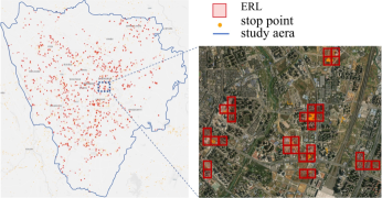
Figure 1: Spatial Distribution of ERLs, (Day shift June 5, 2023)

Figure 2: Number of ERLs on different shifts.

TABLE I: The location category and the corresponding risk level.

Category	Fixd stay locations
ER	Construction sites, Dumping ground
MR	Quarry, Commercial concrete mixing station
PM	Parking lots, Automobile repair station, Maintenance

III-A Basic geographic features

The basic geographic features are related to the structure and location of each ERL. Table II lists the four features. Specifically, $distance\_LR$ denotes the distance between the left and right boundaries. $distance\_UL$ represents the upper and lower boundaries of the sample region. $num\_grid$ indicates the number of $200m\times 200m$ grids in each sample region. $distance\_LR$, $distance\_UL$, and $num\_grid$ provide insights into the approximate shapes and sizes of the ERLs. Additionally, $distance\_center$ represents the Euclidean distance between the geometric center of the ERL and the projected coordinates of the center of Chengdu (Tianfu Square). The size of $distance\_center$ can reflect economic conditions, as Chengdu’s economic planning spreads out in all directions from the center.

TABLE II: Features of geographic.

Features	Description
$num\_grid$	Number of grids
$distance\_LR$	Distance between left and right boundaries
$distance\_UL$	Distance between upper and lower boundaries
$distance\_center$	Distance from city center

III-B Land cover features

Satellite remote-sensing data have achieved good results in the field of location identification and classification [28, 29]. To classify ERLs and reduce data processing costs, we incorporate structured land cover data into the feature set. Table III lists eight common land cover features obtained from [30], with a data resolution of 1 m. To mitigate the influence of the ERL size on the classification results, we calculate the area proportions of the eight land cover features as the final feature. The areas of different ERLs within the same category may vary significantly, potentially resulting in differences of orders of magnitude in land cover features.

TABLE III: Features of land cover.

Features	Description
$traffic\_route$	Area ratio of transportation facilities
$tree\_cover$	Area ratio of trees
$grassland$	Area ratio of low herbaceous
$cropland$	Area ratio of arable land and human planted crops
$building$	Area ratio of human-made building
$barren\_S\_V$	Area ratio of barren and sparse vegetation
$water$	Area ratio of waters
$moss\_lichen$	Area ratio of moss and lichen

III-C POI features

Urban POI data are frequently used as features for urban location identification and classification [31, 32]. POI can be categorized in various ways; we divide them into 17 categories, as listed in Table IV. We calculate the total number of each category of POI within a one-kilometer radius of the geometric center of each ERL, where $all\_poi$ represents the sum of all the POI.

TABLE IV: Features of POI.

Features	Description
$food$	Number of food services within 1km radius
$road\_facility$	Number of road facilities within 1km radius
$scenic\_spots$	Number of scenic spots within 1km radius
$public$	Number of public facilities within 1km radius
$enterprise$	Number of enterprises within 1km radius
$shopping$	Number of shopping services within 1km radius
$trans_{f}acility$	Number of transportation facilities within 1km radius
$financial$	Number of financial services within 1km radius
$science\_E$	Number of science education services within 1km radius
$trans\_F$	Number of transportation facilities within 1km radius
$car\_S$	Number of car services within 1km radius
$car\_R$	Number of car repair Service within 1km radius
$business$	Number of business residences within 1km radius
$subsistence$	Number of subsistence services within 1km radius
$sports$	Number of sports services within 1km radius
$health$	Number of health care services within 1km radius
$government$	Number of government facilities within a radius of 1 km
$Accom$	Number of accommodation services within 1km radius
$all\_poi$	Number of all POI within 1km radius

III-D Dynamic features

ERLs are identified based on the trajectories of dump trucks; therefore, dynamic features such as truck flow and stay points may affect classification accuracy. For instance, PM exhibits a higher outflow during the morning peak and a higher inflow during the evening peak, unlike ER and MR. ER and MR prioritize operational efficiency with shorter stay times for dump trucks, whereas PM experiences longer stay times. Based on dump truck trajectory data, we calculate 20 dynamic features presented in Table V. Here, $flow\_t$ represents the inflow of the ERL during each hour $t$ and $all\_flow$ represents the total flow over the span of 12 h. Meanwhile, $stay\_t$ represents the cumulative number of stopping points within the ERL area for each hour $t$ $(t=1,2,\dots,12)$, and $all\_stay$ represents the total number of stopping points over the course of 12 h. Although the physical meaning of $stay\_t$ is not as explicit as $flow\_10$, it may contain additional information. $degree$ represents the sum of the in- and out-degrees of each ERL, where the degree is the number of edges directly connected to a node. $stay\_time$ represents the average stopping time for all the dump trucks remaining at a specific ERL.

TABLE V: Features of Dynamic.

Features	Description
$stay\_t$	Number of stay points per hour(t=1,2,…,12)
$all\_stay$	Total number of stay points
$flow\_t$	Number of in-flow per hour(t=1,2,…,12)
$all\_flow$	Total number of in-flow
$degree$	Number of in-degrees and out-degrees
$stay\_time$	Average length of stay

IV Classification models and feature importance

In this section, four classification models are introduced for classifying ERLs, and five performance metrics are adopted to address and compare the model performances. Additionally, the SHAP method is introduced for model interpretation, aiming to identify feature importance and demonstrate high classification performance on a more limited subset of features.

IV-A Model

The selection of prediction models can influence prediction performance [33]. We introduce four machine-learning models for the ERL categories: MLP, LR, GBDT, and RF.

IV-A1 Multilayer perceptron

The MLP [23] is a of feedforward neural network with multiple layers. It comprises an input layer, one or more hidden layers, and an output layer. Each layer is composed of multiple neurons that are connected to all the neurons in the preceding layer. Typically, neurons other than the input neurons use nonlinear activation functions, aiding the network in learning more complex mapping relationships. Among them, the commonly used Relu activation function is constructed as

$$Relu(v)=\max(0,v)$$ (1)

where $Relu(v)$ denotes the output and $v$ denotes the input.

For multi-classification problems, the Softmax function is commonly employed for the output layer. The function maps the values of the output neurons to a probability distribution, ensuring that the probability value for each category falls between zero and one and that the sum of the probabilities for all categories is one. The mathematical expression for the Softmax function is

$$Softmax(\mathbf{z}_{i})=\frac{e^{z_{i}}}{\sum_{i}^{K}e^{z_{j}}}$$ (2)

where $\mathbf{z}$ is the input vector, and $K$ is the number of categories.

The cross-entropy loss function(Eq. (3)) is commonly used for multi-classification problems during training. The model parameters are trained using a widely recognized backpropagation algorithm .

$$J(\theta)=-\frac{1}{N}\sum_{i=1}^{N}\sum_{j=1}^{K}y_{ij}log(\hat{y}_{ij})$$ (3)

where $N$ represents the number of samples, $K$ is the number of categories, $y_{ij}$ is the true label (one-hot coding) of sample $i$, and $\hat{y}_{ij}$ is the model’s predicted probability that sample $i$ belongs to category $j$.

IV-A2 Logistic regression

LR is a generalized linear model commonly used to address binary classification problems [23]. Softmax functions can be introduced into the output layer to further expand the generalized LR to Softmax regression, which is suitable for resolving multi-classification problems. Eq (4) represents a generalized LR. The model employs a Softmax function (Eq (2)) at the output layer to translate the raw scores of each category into probabilities, and then determines the model loss based on the cross-entropy loss function (Eq (3)):

$$z_{j}=\mathbf{w}_{j}\mathbf{x}+b_{j}$$ (4)

where $\mathbf{x}$ represents the input feature vector, and $\mathbf{w}_{j}$ and $b_{j}$ are the model coefficients. $z_{j}$ is the output of the linear regression predicting the $j$ category.

IV-A3 Gradient Boosting Decision Trees

GBDT is a versatile nonparametric statistical learning approach extensively used for multi-class classification tasks. The modeling process unfolds in a stepwise manner, enabling the optimization of any differentiable cost function [34]. Similar to other boosting techniques, gradient boosting integrates weak learners iteratively to create a robust learner. By introducing estimator $h$, the refined prediction model is derived as $F_{s+1}(x)=F_{s}(x)+h(x)$. The estimator $h$ is selected as $h(x)=y-F_{s}(x)$, where $y$ is the actual output value.

The GBDT has gained widespread popularity owing to its efficiency, accuracy, and interpretability [34]. It is a promising method for precisely tackling multi-class classification tasks. The GBDT constructs a series of decision trees and statistical models that are tailored for supervised prediction challenges. These trees make predictions through a sequence of decisions outlined in the tree structure, with each node representing a split in the potential values for a specific feature. The utility of decision-tree regression lies in its ease of interpretation and visualization. Moreover, it has the potential to reveal patterns that may be challenging to identify using traditional regression methods. This makes the GBDT a robust choice for efficiently and accurately tackling multi-class classification challenges.

IV-A4 Random forest

The RF is an ensemble prediction model composed of numerous decision trees. Remarkably, RF often yields favorable results, even without extensive hyperparameter tuning [35]. During the training process, each tree in the RF learns from a randomly sampled subset of the data using a bagging technique. Notably, the samples are repeatedly applied within a single tree, resulting in the entire forest having a lower variance without a corresponding increase in bias. RF predictions are derived by averaging the predictions of each decision tree within the ensemble.

Although individual decision trees explore the splits for each feature in every node, RF focuses on a split for only one feature per node. Initially, a small subgroup of explanatory features is randomly selected. Subsequently, the node is split using the best feature from the limited set, and a new set of eligible features is arbitrarily selected. This iterative process continues until the tree is fully grown. Ideally, each terminal node contains only one observation. As the number of features increases, the eligible feature set may differ significantly from one node to another. However, prominent features eventually emerge in the tree, and their respective predictive success enhances the overall reliability.

IV-B Performance metrics

In this section, we compute the confusion matrix (Table VI), where True Positive (TP) denotes the model correctly classifying positive examples as positive, False Positive (FP) represents the model incorrectly classifying negative examples as positive, True Negative (TN) indicates the model correctly categorizing negative cases as negative, and False Negative (FN) signifies the model incorrectly classifying positive examples as negative. Subsequently, we present five predictive performance metrics to assess and compare the performance of the predictive models.

TABLE VI: Confusion Matrix.

	Positive	Negative
Positive	TP	FN
Negative	FP	TN

IV-B1 Accuracy

Accuracy quantifies the overall proportion of correct predictions made by the model, as shown in Eq (5). In situations of category imbalance, the accuracy may be inappropriate, as the model may exhibit a bias towards predicting a higher number of categories.

$$Accuracy=\frac{TP+TN}{TP+TN+FP+FN}$$ (5)

IV-B2 Precision

Precision quantifies the proportion of samples predicted to be positive instances that are positive instances by the model, as depicted in Eq (6). Precision is highly effective for addressing issues that aim to minimize FP instances, such as spam categorization. However, it exhibits less robustness in noisy situations because it concentrates solely on accuracy in positive examples.

$$Precision=\frac{TP}{TP+FP}$$ (6)

IV-B3 Recall

Recall quantifies the proportion of samples that the model successfully predicts as positive among the positive samples, as illustrated in Eq (7). Recall is valuable when addressing the challenge of minimizing FN cases, such as in cancer diagnoses. However, in noisy situations, the occurrence of FPs may increase.

$$Recall=\frac{TP}{TP+FN}$$ (7)

IV-B4 F1-score

The F1-score combines precision and recall and serves as a reconciled average of the two. In the dichotomous case, the F1-score is typically calculated for the category of interest (usually the positive category), and its formula is shown in Eq (8). In the multi-category case, three variants exist: Macro-F1, Micro-F1, and Weighted-F1. Because of the imbalance in the data samples in this study, it is suitable to utilize Macro-F1 for a comprehensive evaluation of the model’s performance, as outlined in Eq (9).

$$F1\text{-}score=\frac{2\times Precision\times Recall}{Precision+Recall}$$ (8)

$$Macro\text{-}F1=\frac{1}{K}\sum_{i=1}^{K}F1\text{-}scrore_{i}$$ (9)

where $K$ is the total number of categories and $F1\text{-}score_{i}$ is the F1-score of the $kth$ category.

IV-B5 AUROC

The receiver operating characteristic (ROC) curve evaluates the performance of the classification model across various classification thresholds. The curve represents the True Positive Rate (TPR, as shown in Eq (10)) on the Y-axis and the False Positive Rate (FPR, as shown in Eq (11)) on the X-axis. Proximity to the upper-left corner indicates better model performance, with no impact of sample imbalance on the ROC curve. The area under the curve (AUC) represents the area beneath the ROC curve; the closer the AUC is to 1, the better the model performance.

$$TPR=\frac{TP}{TP+FN}$$ (10)

$$FPR=\frac{FP}{FP+TN}$$ (11)

IV-C Feature importance

The SHAP method, which is rooted in cooperative game theory and based on Shapley values, serves as an approach for interpreting machine learning models [25]. SHAP represents the output model as a linear summation of the input variables. Assuming that the input variable of the model is $\mathbf{x}$, the interpretive model $g(\mathbf{x}^{{}^{\prime}})$ of the original model $f(\mathbf{x})$ is denoted by

$$f(\mathbf{x})=g(\mathbf{x}^{{}^{\prime}})=\phi_{0}+\sum_{i=1}^{M}\phi_{i}x_{i}^{{}^{\prime}}$$ (12)

where $\mathbf{x}^{{}^{\prime}}$ represents the simplified input, $M$ represents the number of input features, and $\phi_{0}$ represents the output value of the model when all the inputs are missing. The inputs $\mathbf{x}^{{}^{\prime}}$ and $\mathbf{x}$ are related by the mapping function $\mathbf{x}=h_{x}(\mathbf{x}^{{}^{\prime}})$. Eq (12) has a unique solution and exhibits three ideal properties: local accuracy, missingness, and consistency. The only possible model that satisfies these properties is:

$$\phi_{i}(f,\mathbf{x})=\sum_{\mathbf{z}^{{}^{\prime}}\subseteq\mathbf{x}^{{}^{\prime}}}\frac{|\mathbf{z}^{{}^{\prime}}|!(M-|\mathbf{z}^{{}^{\prime}}|-1)!}{M!}[f_{x}(\mathbf{z}^{{}^{\prime}})-f_{x}(\mathbf{z}^{{}^{\prime}}\backslash i)]$$ (13)

where $|\mathbf{z}^{{}^{\prime}}|$ represents the number of non-zero entries in $\mathbf{z}^{{}^{\prime}}$. $\phi_{i}$ is the Shaply value from Eq (12) and $\mathbf{z}^{{}^{\prime}}\backslash i$ represents $z_{i}^{{}^{\prime}}=0$. $f_{x}(\mathbf{z}^{{}^{\prime}})=f(h_{x}(\mathbf{z}^{{}^{\prime}}))=E[f(\mathbf{z})|\mathbf{z}_{s}]$ and $S$ is the set of nonzero indices in $\mathbf{z}^{{}^{\prime}}$, known as SHAP values.

SHAP provides effective explanations for both local and global model interpretations. In this study, we employ the method proposed by [26] for Shapley value calculations tailored to tree models, reducing the computational complexity from $O(TL2^{M})$ to $O(TLD^{2})$ where $T$ is the number of trees, $L$ is the maximum number of leaves in any tree, $M$ is the number of features, and $D$ is the maximum depth of any tree. Calculating feature importance serves two purposes: to analyze the contribution of each feature to predictions for model interpretation, feature selection, and performance improvement; and to analyze ERL features to create a characteristic profile for ERLs, aiding in understanding ERL operational patterns. This will facilitate relevant authorities in formulating targeted control measures and lay the groundwork for further research.

V Results: model configuration and tuning

In this section, we first present the experimental sets and then report the predictive performances of several models. Our goal was to determine the model with the highest predictive performance before investigating the importance of the features.

V-A Experimental setup

Four classification models were implemented using the Scikit-Learn library in Python. The parameters for LR, MLP, GBDT, and RF were set as follows: for LR, the maximum number of iterations, regularization strength coefficient, and classification weight coefficients were 800, 1.0, and 0.2:0.5:0.3, respectively; for MLP: the activation function, size of the hidden layer, learning rate, and maximum number of iterations were Relu, [256,128], 0.01, 800, and 1.3, respectively; for GBDT: the maximum number of iterations, L2 penalty parameter, learning rate, and maximum depth were 100, 10, 0.01, and 6, respectively; and for RF: the number of trees, maximum depth, and classification weights were 150, 7, and 0.2:0.5:0.3, respectively. To ensure experimental comparability, the same random seeds were applied to all four classification models throughout the experiment. In each experiment, the datasets of the four models were identical.

Detailed information regarding the experimental data is provided in Section V-B. Given that samples from different shifts may belong to the same ERL, the division of the training and validation sets should be based on the 2,403 known ERLs in the ERL registry, rather than on the 20,489 samples over 64 shift times. We randomly selected 70% as the training set, 10% as the validation set, and 20% as the test set from the ERL registry. The model results for the 20% unseen test set are listed in Table VII.

V-B Performance of different models

Table VII presents a comparison of the four models—LR, SF, MLP, and GBDT—across the five performance metrics. Overall, RF demonstrated the best performance. The RF model exhibited strong performance across all five metrics, presenting notable improvements compared to the traditional subjective manual evaluation. Notably, the model’s slightly lower Recall and F1 scores may be attributed to the relatively small sample sizes of categories MR and PM. Despite the application of higher weights, the model’s learning of categories MR and PM remained constrained. LR proved to be the least effective among the four models, primarily because the simplicity of the linear model hinders its ability to fully explore the complex mapping relationship between features and target labels. RF excels not only in performance but also exhibits strong model interpretability. Consequently, we selected RF as the final model for subsequent feature-importance experiments.

TABLE VII: Comparison of the performance of five evaluation metrics for ERL classification is presented, including mean and standard deviation. The best performance is highlighted in bold.

Model	Accuracy	Precision	Recall	Macro-F1	AUROC
LR	0.663$\pm$0.007	0.483$\pm$0.016	0.427$\pm$0.008	0.429$\pm$0.011	0.722$\pm$0.009
MLP	0.756$\pm$0.017	0.754$\pm$0.016	0.568$\pm$0.019	0.597$\pm$0.023	0.837$\pm$0.012
GBDT	0.778$\pm$0.012	0.814$\pm$0.019	0.541$\pm$0.015	0.583$\pm$0.026	0.862$\pm$0.013
RF	0.785$\pm$0.014	0.803$\pm$0.018	0.569$\pm$0.017	0.609$\pm$0.021	0.870$\pm$0.011

VI Results: feature importance

In this section, we examine the relationship between different features and target labels using the SHAP-values and feature distributions. One of our goals is to clarify the importance of features in constructing a more streamlined classification model. The second goal is to mine the operational rules of ERLs so that the relevant authorities can formulate targeted regulatory measures.

VI-A Feature importance analysis

As discussed in Section IV-C, extracting the feature importance from classification models is a crucial process. Fig. 3 depicts the importance ranking of 58 features in the RF model as determined by the SHAP-values. In Fig. 3, the vertical axis represents various features and the horizontal axis represents the sum of the absolute SHAP values for all samples—the feature importance values. The sum of the importance values for all the features was normalized to 1. For a more comprehensive understanding and evaluation of the importance values, Fig. 4 summarizes the SHAP-values for the top 15 features, each with an importance value exceeding 0.02. Each data point represents a sample, where blue indicates smaller feature values and red indicates larger feature values. The relationship between the sample and SHAP values is depicted in Fig. 4. To provide a more intuitive understanding of the differences in the feature values among the different categories, Fig. 5 shows the numerical distributions of the top 15 features.

The $distance\_center$ in the basic geographic features, representing the distance of the samples from the city center, is the most crucial for predictions across different categories. This is particularly evident when predicting ER, where the importance value of $distance\_center$ is notably higher than that of the other features. This observation is consistent with the results presented in Figs. 4 and 5(a), that is, as the sample proximity to the city center increases, the probability of it belonging to ER is higher, followed by MR, and finally PM. This pattern is likely attributable to the distribution of construction sites in ER, which are typically spread across the city. By contrast, MR sites (quarry, commercial concrete mixing station) and parking lots are constrained from being located in the city center. Conversely, parking lots tend to be situated farther away from the city center. This conclusion aligns with urban planning principles [36].

Among the dynamic features, $stay\_time$, $all\_flow$ (total inflow within one shift), and $stay\_10$ (total number of stay points in the 10th hour of a shift) demonstrated higher importance values. As shown in Figs. 4 and 5 (b,g,n), for $stay\_time$, the main reason is that dump trucks stay in the parking lot for a longer period. For $all\_flow$, this may be attributed to the fact that the flow of dump trucks in construction sites, quarries, and commercial mixing concrete stations is typically determined by the workload; therefore, the inflow is generally not very high. However, parking lots often accommodate dump trucks from other ERLs, resulting in relatively large flows. For $stay\_10$, the 10th hour of a shift typically marks the end of the working day, and dump trucks primarily transition from work areas to parking lots. Consequently, the $stay\_10$ in parking lots is larger, $stay\_10$ for ER is smaller, and for MR-possibly due to the smaller amount of data—the feature importance of $stay\_10$ is lower. Interestingly, the importance value of $stay\_10$ exceeds that of $flow\_10$. As discussed in Section III-D, although the physical meaning of $stay\_10$ is not as explicit as that of $flow\_10$, it may contain additional information. Fig. 3 also indicates that the feature importance values of $flow\_t(t=1,2,\dots,12)$ are generally low. This may be attributed to the inherent randomness in the operations of dump trucks, which lack unified and effective regulation. This may be attributed to the strong randomness in the operations of dump trucks, which lacks unified and effective regulation during the working period. The typical operating modes are ”first come, first load,” ”first come, first unload,” and ”arrive later, queue up,” and evaluating the travel and queue times on the road is challenging.

Within the land cover feature, $grassland$ exhibited a high importance value, whereas the remaining features demonstrated a lower performance. As shown in Figs. 4 and 5 (d), samples with a larger $grassland$ feature were more likely to be predicted as MR and, conversely, as in other categories. This may be because the dumping ground in ER is usually located in the outer suburbs and the land surface is not treated, thus preserving the original $grassland$. By contrast, quarries, commercial concrete mixing stations, and parking lots are also located in the outer suburbs, but their land surfaces are usually treated, and almost no $grassland$ is preserved. Fig. 3 indicates that several other land cover features have lower importance values. Previous studies [28, 29] have successfully used urban satellite remote sensing data to identify and classify urban locations. The relatively low importance values of land-cover features in this study suggest that structured land-cover data may not capture sufficient information to compete with remotely sensed image data.

The importance values of the POI features are generally high, particularly for features such as $all\_poi$, $business$, $road\_fac$, $health$. As observed in Figs. 4 and 5, the number of POI in each category around MR is the smallest, followed by PM, and finally ER. Although we categorized POI into 17 categories, numerous other criteria for categorizing POI exist, and other categories of POI data are worth considering.

Figure 3: Feature importance ranking for different categories of samples.

Figure 4: Feature importance analysis with all samples for three categories.

Figure 5: Distribution of features in different categories.

VI-B Model simplification

Dependencies exist among the features, and the removal of certain features leads to changes in the importance values of the remaining features. Specifically, as illustrated by the ordering of importance values in Fig.  3, features such as $moss\_lichen,flow\_6,\dots,flow\_11$ exhibit low importance values; therefore, these features were simultaneously removed. Then, $stay\_4,stay\_1,\dots,stay\_time,distance\_center$ was removed and the changes in the values of the five performance metrics were dynamically recorded; the results are shown in Fig. 6.

In Fig. 6, the horizontal axis, which progresses from left to right, represents the gradual removal of features, and the vertical axis denotes the values of the model performance metrics. The points marked by black circles indicate instances where the model performance begins to decline significantly, with slight variations in the points at which different performance metrics decrease. The precision initially experiences a significant drop, whereas the recall exhibits a corresponding slow upward trend. In addition, Macro-F1 remains almost unchanged, making it suitable for practical applications. Many studies regard Macro-F1 as a measure of the comprehensive performance of the model; therefore, our RF model only needs to retain the six features $distance\_center$, $stay\_time$, $all\_poi$, $grassland$, $business$, and $road\_fac$ to achieve a high level of performance.

Figure 6: Prediction performance for iteratively reducing features until all features are removed (i.e., until random guessing). Black circles denote the prediction performance of the current performance metric with a smaller subset of features.

VII Real-world deployment

The ERL classification algorithm was successfully deployed in the Alpha-MAPS Intelligent Atmospheric Monitoring and Control System ($AM\_System$) by the end of November 2023. The $AM\_System$ was implemented in Chengdu (a megacity in China) starting in March 2022, and has played a significant role in urban environmental monitoring and governance [37].

For each run, the ERL classification algorithm utilizes the trajectories of dump trucks from the previous 60 days, POI data, and land cover data to predict the category of ERL on that day. Subsequently, it generates the verification tasks to be assigned to the inspectors. Upon receiving the task, inspectors carry the drone to the ERL site, record and upload relevant information such as the ERL’s image, category, size, working status, and whether it is conducting environmental operations. This information is then used as a government decision support and to update the ERLs classification model.

In December 2023, 30,785 ERLs were identified. Of these, 16,132 ERLs belong to unknown categories. Owing to resource constraints, inspectors conducted 1,092 manual field verifications and achieved a classification accuracy of 77.8%. Notably, the same ERL can be counted repeatedly in different shifts, which is permissible in real-world scenarios. Fig. 7 depicts the ERL site photos uploaded to $AM\_system$ by inspectors (privacy information has been coded).

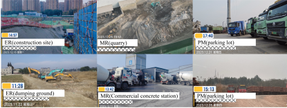
Figure 7: Site photos by inspectors for site verification, uploaded to $AM\_system$.

VIII Conclusion

This study aimed to develop a classification model for urban dust pollution sources by introducing a set of features that could potentially influence dust pollution sources. These features include basic geographic features, land cover features, urban POI features, and dump truck dynamic features. Using real data from Chengdu City, we aimed to establish the most suitable classification model for urban dust pollution sources. Comparative experiments involving four machine learning models revealed that the RF model outperformed the other models regarding classification effectiveness.

A key aspect of this study is the identification of feature importance and model simplification. The feature importance identification relies on the SHAP-value method, whereas model simplification combines the SHAP-value and backward elimination methods. Quantitative analysis indicated that $distance\_center$(the distance of samples from the city center) was the most crucial feature, followed by $stay\_time$, $all\_poi$(number of all POI within a 1km radius), and $grassland$(area ratio of low herbaceous). Furthermore, feature importance analysis not only aids in comprehending the operational patterns of dust pollution sources but also guides model simplification. The results of the model simplification demonstrate that high-accuracy classification can be achieved using only a small subset of features, including $distance\_center$, $stay\_time$, $all\_poi$, $grassland$, $business$, and $road\_fac$.

Future research on urban dust pollution sources can progress in several directions. (1) More urban data can be gathered and the classification model can be tailored to meet the environmental regulatory needs of different cities within the framework of this study. (2) Additional machine learning methods can be considered, such as lasso regression and support vector machines, and deep learning methods can be explored. (3) The feature set can be expanded to encompass the multifaceted characteristics of dust pollution sources. (4) A model for evaluating and controlling urban dust pollution sources can be constructed by combining active time and in/outflow data for a comprehensive assessment and ranking of dust risks. We acknowledge that despite the considerable progress made in this study, there is still potential for further improvement in the model accuracy, and pursuing these directions may prove to be an effective means of achieving this goal.

References

- [1] Z. Wu, X. Zhang, and M. Wu, “Mitigating construction dust pollution: State of the art and the way forward,” Journal of Cleaner Production, vol. 112, pp. 1658–1666, 2016.
- [2] Ministry of Ecology and Environment of the People’s Republic of China, “2020 China ecological status environmental bulletin,” [Online]. Available: https://www.mee.gov.cn/hjzl/sthjzk/zghjzkgb/
- [3] D. Cheriyan and J.-h. Choi, “A review of research on particulate matter pollution in the construction industry,” Journal of Cleaner Production, vol. 254, p. 120077, 2020.
- [4] X. Li, Y. Zhu, and Z. Zhang, “An lca-based environmental impact assessment model for construction processes,” Building and Environment, vol. 45, no. 3, pp. 766–775, 2010.
- [5] K. Han, Z. Yang, C. Chen, X. Liu, B. Zhao, W. Li, and Y. Wang, “Research on digital intelligent supervision and carbon reduction of construction waste trucks: A case study of chengdu city,” Dec. 2023. [Online]. Available: https://www.researchgate.net/publication/376354707
- [6] M. Ghasemi, D. Toghraie, and A. Abdollahi, “An experimental study on airborne particles dispersion in a residential room heated by radiator and floor heating systems,” Journal of Building Engineering, vol. 32, p. 101677, 2020.
- [7] J. Hong, H. Kang, S. Jung, S. Sung, T. Hong, H. S. Park, and D.-E. Lee, “An empirical analysis of environmental pollutants on building construction sites for determining the real-time monitoring indices,” Building and Environment, vol. 170, p. 106636, 2020.
- [8] H. Yan, G. Ding, K. Feng, L. Zhang, H. Li, Y. Wang, and T. Wu, “Systematic evaluation framework and empirical study of the impacts of building construction dust on the surrounding environment,” Journal of Cleaner Production, vol. 275, p. 122767, 2020.
- [9] Q. Luo, L. Huang, X. Xue, Z. Chen, F. Zhou, L. Wei, and J. Hua, “Occupational health risk assessment based on dust exposure during earthwork construction,” Journal of Building Engineering, vol. 44, p. 103186, 2021.
- [10] P. Faber, F. Drewnick, and S. Borrmann, “Aerosol particle and trace gas emissions from earthworks, road construction, and asphalt paving in germany: Emission factors and influence on local air quality,” Atmospheric Environment, vol. 122, pp. 662–671, 2015.
- [11] S. Gautam and A. K. Patra, “Dispersion of particulate matter generated at higher depths in opencast mines,” Environmental Technology & Innovation, vol. 3, pp. 11–27, 2015.
- [12] S. Ahmed and I. Arocho, “Emission of particulate matters during construction: A comparative study on a cross laminated timber (clt) and a steel building construction project,” Journal of Building Engineering, vol. 22, pp. 281–294, 2019.
- [13] B. Li, Y. Ouyang, X. Li, D. Cao, T. Zhang, and Y. Wang, “Mixed-integer and conditional trajectory planning for an autonomous mining truck in loading/dumping scenarios: A global optimization approach,” IEEE Transactions on Intelligent Vehicles, vol. 8, no. 2, pp. 1512–1522, 2022.
- [14] N. Deng, X. Li, and Y. Su, “Optimization of earthwork allocation path as vehicle route problem based on genetic algorithm,” in E3S Web of Conferences, vol. 165. EDP Sciences, 2020, p. 04057.
- [15] K. Han and C. Chen, “Method for deducing pollution point location based on slag transport vehicle track point,” Patent CN115 964 545B, Apr. 2023. [Online]. Available: https://patents.google.com/patent/CN115964545B/en
- [16] K. Han, Y. Wang, and C. Chen, “A method for identifying earthwork points and transportation networks based on gps trajectories of slag trucks,” Patent CN117 131 149B, Jan. 2024. [Online]. Available: https://www.patentguru.com/cn/CN117131149B/en
- [17] V. Mayer-Schönberger and K. Cukier, Big data: A revolution that will transform how we live, work, and think. Houghton Mifflin Harcourt, 2013.
- [18] A. McAfee, E. Brynjolfsson, T. H. Davenport, D. Patil, and D. Barton, “Big data: the management revolution,” Harvard Business Review, vol. 90, no. 10, pp. 60–68, 2012.
- [19] W. Lu, “Big data analytics to identify illegal construction waste dumping: A hong kong study,” Resources, Conservation and Recycling, vol. 141, pp. 264–272, 2019.
- [20] J. Bi, Q. Sai, F. Wang, Y. Chen et al., “Identification of working trucks and critical path nodes for construction waste transportation based on electric waybills: A case study of Shenzhen, China,” Journal of Advanced Transportation, vol. 2022, 2022.
- [21] J. Ji, J. Wang, J. Wu, B. Han, J. Zhang, and Y. Zheng, “Precision cityshield against hazardous chemicals threats via location mining and self-supervised learning,” in Proceedings of the 28th ACM SIGKDD Conference on Knowledge Discovery and Data Mining, 2022, pp. 3072–3080.
- [22] M. Mohammed, M. B. Khan, and E. B. M. Bashier, Machine learning: algorithms and applications. CRC Press, 2016.
- [23] J. Han, J. Pei, and H. Tong, Data mining: concepts and techniques. Morgan Kaufmann, 2022.
- [24] I. H. Witten and E. Frank, “Data mining: practical machine learning tools and techniques with java implementations,” ACM Sigmod Record, vol. 31, no. 1, pp. 76–77, 2002.
- [25] S. M. Lundberg and S.-I. Lee, “A unified approach to interpreting model predictions,” Advances in neural information processing systems, vol. 30, 2017.
- [26] S. M. Lundberg, G. G. Erion, and S.-I. Lee, “Consistent individualized feature attribution for tree ensembles,” arXiv preprint arXiv:1802.03888, 2018.
- [27] L. S. Shapley et al., “A value for n-person games,” 1953.
- [28] C. Chen, J. Yan, L. Wang, D. Liang, and W. Zhang, “Classification of urban functional areas from remote sensing images and time-series user behavior data,” IEEE Journal of Selected Topics in Applied Earth Observations and Remote Sensing, vol. 14, pp. 1207–1221, 2020.
- [29] P. Lynch, L. Blesius, and E. Hines, “Classification of urban area using multispectral indices for urban planning,” Remote Sensing, vol. 12, no. 15, p. 2503, 2020.
- [30] Z. Li, W. He, M. Cheng, J. Hu, G. Yang, and H. Zhang, “Sinolc-1: the first 1-meter resolution national-scale land-cover map of China created with the deep learning framework and open-access data,” Earth System Science Data Discussions, vol. 2023, pp. 1–38, 2023.
- [31] M. Zheng, H. Wang, Y. Shang, and X. Zheng, “Identification and prediction of mixed-use functional areas supported by poi data in Jinan city of China,” Scientific Reports, vol. 13, no. 1, p. 2913, 2023.
- [32] G. Luo, J. Ye, J. Wang, and Y. Wei, “Urban functional zone classification based on poi data and machine learning,” Sustainability, vol. 15, no. 5, p. 4631, 2023.
- [33] X. Wang, A. E. Brownlee, J. R. Woodward, M. Weiszer, M. Mahfouf, and J. Chen, “Aircraft taxi time prediction: Feature importance and their implications,” Transportation Research Part C: Emerging Technologies, vol. 124, p. 102892, 2021.
- [34] G. Ke, Q. Meng, T. Finley, T. Wang, W. Chen, W. Ma, Q. Ye, and T.-Y. Liu, “Lightgbm: A highly efficient gradient boosting decision tree,” Advances in neural information processing systems, vol. 30, 2017.
- [35] S. Bernard, L. Heutte, and S. Adam, “Influence of hyperparameters on random forest accuracy,” in Multiple Classifier Systems: 8th International Workshop, MCS 2009, Reykjavik, Iceland, June 10-12, 2009. Proceedings 8. Springer, 2009, pp. 171–180.
- [36] W. Peng, G. Wang, J. Zhou, J. Zhao, and C. Yang, “Studies on the temporal and spatial variations of urban expansion in Chengdu, western China, from 1978 to 2010,” Sustainable Cities and Society, vol. 17, pp. 141–150, 2015.
- [37] Sichuan Guolan Zhongtian Environmental Technology Group Co Ltd, “Alpha-maps intelligent atmospheric monitoring and control system,” [Online]. Available: https://marketplace.huaweicloud.com/contents/a6cc6b5a-6f62-4509-867e-b7e4395b3ca3#productid=OFFI858632267563057152