Bayesian Off-Policy Evaluation and Learning for Large Action Spaces

Abstract

In interactive systems, actions are often correlated, presenting an opportunity for more sample-efficient off-policy evaluation (OPE) and learning (OPL) in large action spaces. We introduce a unified Bayesian framework to capture these correlations through structured and informative priors. In this framework, we propose sDM, a generic Bayesian approach designed for OPE and OPL, grounded in both algorithmic and theoretical foundations. Notably, sDM leverages action correlations without compromising computational efficiency. Moreover, inspired by online Bayesian bandits, we introduce Bayesian metrics that assess the average performance of algorithms across multiple problem instances, deviating from the conventional worst-case assessments. We analyze sDM in OPE and OPL, highlighting the benefits of leveraging action correlations. Empirical evidence showcases the strong performance of sDM.

1 Introduction

An off-policy contextual bandit (Dudík et al., 2011) is a practical framework for improving decision-making using logged data. In practice, we often have access to logged data that summarizes an agent’s interactions with an online environment (Bottou et al., 2013). This data is typically in the form of context-action-reward tuples, where each interaction round involves the agent observing a context, taking an action, and receiving a reward that depends on the observed context and the taken action. This data provides valuable insights that can be leveraged to improve the performance of the agent. This process involves two primary tasks. First, there is off-policy evaluation (OPE) (Dudík et al., 2011), which allows predicting the expected reward of a new policy using logged data. Second, off-policy learning (OPL) where this same estimator is used to improve the agent’s decision-making policy (Swaminathan & Joachims, 2015a). Many interactive systems (e.g., online advertising, music and video streaming) can be modeled as contextual bandits. Consider online advertising as an example. Here, the context is the user’s features, the action is a product choice, and the reward is the click-through rate (CTR).

When the number of actions is small, existing methods for OPE and OPL, which are often based on the inverse propensity scoring (IPS) estimator (Horvitz & Thompson, 1952), are reliable with good theoretical guarantees (Dudík et al., 2011, 2012; Dudik et al., 2014; Wang et al., 2017; Farajtabar et al., 2018; Su et al., 2019, 2020; Metelli et al., 2021; Swaminathan & Joachims, 2015a; London & Sandler, 2019; Aouali et al., 2023a). Unfortunately, IPS uses the importance sampling trick and it is known to suffer high bias and variance in practice. The bias is due to the fact that the logging policy might have deficient support (Sachdeva et al., 2020), while the variance issue is related to the high values of the importance weights. Both problems are more pronounced when the number of actions is large. The variance issue of IPS is acknowledged in the literature and several methods have been proposed to mitigate it (e.g., Hanna et al. (2019); Schlegel et al. (2019); De Asis et al. (2023); Aouali et al. (2023a) and references therein). Still, these approaches fail in large action spaces. Recently, Saito & Joachims (2022) proposed marginalized IPS (MIPS) to scale IPS to OPE tasks involving large action spaces. However, MIPS was previously explored exclusively in OPE and relies on predefined and observed action embeddings, which directly impact the reward. Note that the existence of such observed action embeddings that have a direct effect on reward may not always hold true in practice.

An alternative to IPS is the direct method (DM) (Jeunen & Goethals, 2021). DMs take a different approach by not relying on importance sampling. Instead, they learn a model that can approximate the expected reward for any given context-action pair, and this model is used to evaluate policies. Generally, DMs tend to introduce less variance compared to IPS, but they can also suffer higher bias when the model is not a perfect fit for the data. While IPS has been a primary focus in the literature due to concerns about their modeling bias, DMs are widely used in practical applications, especially in large-scale recommender systems (Sakhi et al., 2020; Jeunen & Goethals, 2021; Aouali et al., 2022). This work aims to establish the algorithmic and theoretical foundations for DMs, improving our understanding of their performance in OPE and OPL. The goal is to enhance the effectiveness of DMs, particularly in scenarios with large action spaces. Note that some prior works suggest combining IPS with DM, such as Doubly Robust (DR) (Dudík et al., 2011). While this combination can reduce variance in practice, it tends to perform less optimally when dealing with large action spaces (Saito & Joachims, 2022). Furthermore, DR itself relies on DM, emphasizing the significance of advancing DM techniques.

Contributions. As previously stated, we focus on DMs; for which we develop both algorithmic and theoretical foundations, particularly in large action spaces. First, we introduce a generic Bayesian DM, denoted as sDM, designed for both OPE and OPL. sDM effectively captures the underlying problem structure through the use of informative priors, facilitating the exchange of information among actions. Essentially, when one action is observed, it contributes to the agent’s knowledge about related actions, significantly enhancing statistical efficiency while keeping computational efficiency intact. This makes sDM scalable to large action spaces which addresses an important limitation of IPS and standard DMs. Additionally, we offer a comprehensive step-by-step framework to assist practitioners in using sDM for OPE and OPL applications. To establish theoretical guarantees for sDM, we introduce the Bayesian Suboptimality (BSO) metric, designed to demonstrate the advantages of incorporating informative priors. Similar to Bayesian regret in online bandits, BSO assesses algorithmic performance across various problem instances, diverging from traditional worst-case evaluations. This contribution signifies an advancement in our comprehension of DMs, particularly within the domain of OPL, where statistical analysis of DMs remains relatively underdeveloped, except for a few recent exceptions (Hong et al., 2023). Finally, we evaluate sDM using both synthetic and MovieLens data, showcasing its robust performance.

Related work. Bayesian models for OPL have been explored by Lazaric & Ghavamzadeh (2010); Hong et al. (2023). However, these works incorporate Bayesian techniques within the context of multi-task learning, distinguishing them from our more focused single-task approach. Additionally, the models used in these prior works differ from the ones we employ. While certain similarities can be drawn with Hong et al. (2023) in terms of analysis, our approach offers a broader scope. Note that Hong et al. (2023) also introduced a Bayesian metric for assessing suboptimality, yet their metric evaluates performance in an environment drawn from the prior given a fixed sample set, whereas ours measures average performance across all environments sampled from the prior and all sample sets. The latter is more common in Bayesian analyses (e.g., Bayesian regret in Russo & Van Roy (2014)). Also, in this work, we cover OPE which goes beyond the scope of Lazaric & Ghavamzadeh (2010); Hong et al. (2023) that focused on OPL. For a more extensive exploration of related works, refer to Appendix B.

The remainder of the paper is organized as follows. Section 2 provides some background on OPE and OPL. Section 3 describes our method, sDM. Section 4 focuses on two special instances of sDM, with either linear or non-linear rewards. One leads to closed-form solutions while the other requires approximation. In Section 5 we analyze sDM showcasing its benefits. Finally, in Section 6, we show that sDM enjoys favorable performance in practice.

2 Background

Let $[n]=\{1,\dots,n\}$ for any positive integer $n$. Random variables are denoted with capital letters, and their realizations with the respective lowercase letters, except for Greek letters. Let $X,Y$ be two random variables, with a slight abuse of notation, the distribution (or density) of $X\mid Y=y$ evaluated at $x$ is denoted by $p(x\mid y)$. Let $a_{1},\ldots,a_{n}$ be $n$ vectors of ^d, $a=(a_{i})_{i\in[n]}\in^{nd}$ is their $nd$-dimensional concatenation. We use $\otimes$ to denote the Kronecker product and $\mathcal{O}$ for the big-O notation. Finally, for any vector $a\in^{d}$ and any positive-definite matrix $\Sigma\in^{d\times d}$, we define $\|a\|_{\Sigma}=\sqrt{a^{\top}\Sigma a}$.

Agents are represented by stochastic policies $\pi\in\Pi$, where $\Pi$ is the set of policies. Precisely, given a context $x\in^{d}$, $\pi(\cdot\mid x)$ is a probability distribution over a finite action set $\mathcal{A}=[K]$, where $K$ is the number of actions. Agents interact with a contextual bandit environment over $n$ rounds as follows. In round $i\in[n]$, the agent observes a context $X_{i}\sim\nu$, where $\nu$ is a distribution whose support $\mathcal{X}$ is a compact subset of $\mathbb{R}^{d}$. Then the agent takes an action $A_{i}\sim\pi_{0}(\cdot\mid X_{i})$ from the action set $\mathcal{A}$, where $\pi_{0}$ is the logging policy. Finally, assuming a parametric model, the agent receives a stochastic reward $R_{i}\sim p(\cdot\mid X_{i};\theta_{*,A_{i}})$. Here $p(\cdot\mid x;\theta_{*,a})$ is the reward distribution for action $a$ in context $x$, where $\theta_{*,a}\in^{d}$ is an unknown $d$-dimensional parameter of action $a$. Let $\theta_{*}=(\theta_{*,a})_{a\in\mathcal{A}}\in^{dK}$ be the concatenation of action parameters. Then, $r(x,a;\theta_{*})=\mathbb{E}_{R\sim p(\cdot\mid x;\theta_{*,a})}\left[R\right]$ is the reward function that outputs the expected reward of action $a$ in context $x$. Finally, the goal is to find a policy $\pi\in\Pi$ that maximizes the value function

$$\textstyle V(\pi;\theta_{*}) \textstyle=\mathbb{E}_{X\sim\nu}\mathbb{E}_{A\sim\pi(\cdot|x)}\left[r(X,A;\theta_{*})\right]\,.$$ (1)

Let $S=(X_{i},A_{i},R_{i})_{i\in[n]}$ be a set of random variables drawn i.i.d. as $X_{i}\sim\nu$, $A_{i}\sim\pi_{0}(\cdot\mid X_{i})$ and $R_{i}\sim p(\cdot\mid X_{i};\theta_{*,A_{i}})$. The goal of off-policy evaluation (OPE) and learning (OPL) is to build an estimator $\hat{V}(\pi,S)$ of $V(\pi;\theta_{*})$ and then use $\hat{V}(\pi,S)$ to find a policy $\hat{\pi}\in\Pi$ that maximizes $V(\cdot;\theta_{*})$. In OPE, it is common to use inverse propensity scoring (IPS) (Horvitz & Thompson, 1952; Dudík et al., 2012), which leverages importance sampling to estimate the value $V(\pi;\theta_{*})$ as $\hat{V}_{\textsc{ips}}(\pi,S)=\frac{1}{n}\sum_{i\in[n]}\frac{\pi(A_{i}\mid X_{i})}{\pi_{0}(A_{i}\mid X_{i})}R_{i}$ where for any $(x,a)\in\mathcal{X}\times\mathcal{A}\,,\frac{\pi(a\mid x)}{\pi_{0}(a\mid x)}$ are the importance weights. In practice, IPS can suffer high variance, especially when the action space is large (Swaminathan et al., 2017; Saito & Joachims, 2022). Moreover, while IPS is unbiased under the assumption that the logging policy has full support, it can induce a high bias when such an assumption is violated (Sachdeva et al., 2020), which is again likely when the action space is large. IPS, also, assumes access to the logging policy $\pi_{0}$. An alternative approach to IPS is to use a direct method (DM) (Jeunen & Goethals, 2021), that relies on a reward model $\hat{r}$ to estimate the value $V(\pi;\theta_{*})$ as

$$\textstyle\hat{V}_{\textsc{dm}}(\pi,S) \textstyle=\frac{1}{n}\sum_{i\in[n]}\sum_{a\in\mathcal{A}}\pi(a\mid X_{i})\hat{r}(X_{i},a)\,,$$ (2)

Here, $\hat{r}(x,a)$ is an estimation of $r(x,a;\theta_{*})$. It’s worth noting that, while DM estimators may also exhibit bias due to the choice of the reward model, they generally have lower variance than IPS estimators (Saito & Joachims, 2022). One notable advantage of DM is its practical utility and its ability to operate without requiring access to the logging policy $\pi_{0}$ (Aouali et al., 2022). Additionally, DMs can be incorporated into a Bayesian framework, where we can leverage informative priors to enhance statistical efficiency. This approach allows for the development of scalable methods suitable for large action spaces, as demonstrated in our work.

3 Approach

In this section, we present a unified Bayesian approach for DM that captures action correlations and hence uses the sample set more efficiently. But before doing that, we start by describing the pitfalls of using standard DMs that discard action correlations.

3.1 Pitfalls of Standard Priors

Consider the following widely used prior

$$\textstyle\theta_{a} \textstyle\sim\mathcal{N}(\mu_{a},\Sigma_{a})\,, \textstyle\forall a\in\mathcal{A}\,,$$ (3)

$$\textstyle R\mid\theta,X,A \textstyle\sim\mathcal{N}(\phi(X)^{\top}\theta_{A},\sigma^{2})\,,$$

where $\phi(X)$ outputs a $d$-dimensional representation of the context $X\in\mathcal{X}$, $\mathcal{N}(\mu_{a},\Sigma_{a})$ is the prior density of $\theta_{a}$, and $\sigma^{2}$ is the reward noise variance. In this prior, each action $a$ corresponds to a parameter $\theta_{a}$.

Assumption 3.1 (Independence).

$(X,A)$ is independent of $\theta$. Also, the $\theta_{a}$, for $a\in\mathcal{A}$ are independent.

Then, under the prior in (3) and 3.1, the posterior on an action parameter is also a multivariate Gaussian and writes $\theta_{a}\mid S\sim\mathcal{N}(\hat{\mu}_{a},\hat{\Sigma}_{a})\,,$ where

$$\textstyle\hat{\Sigma}_{a}^{-1}=\Sigma_{a}^{-1}+G_{a}\,, \textstyle\hat{\Sigma}_{a}^{-1}\hat{\mu}_{a}=\Sigma_{a}^{-1}\mu_{a}+B_{a}\,,$$ (4)

where $G_{a}=\sigma^{-2}\sum_{i\in[n]}\mathbb{I}_{\{A_{i}=a\}}\phi(X_{i})\phi(X_{i})^{\top}$ and $B_{a}=\sigma^{-2}\sum_{i\in[n]}\mathbb{I}_{\{A_{i}=a\}}R_{i}\phi(X_{i})$. Note that $G_{a}$ and $B_{a}$ only use the portion of the sample set $S$ where action $a$ was observed. Thus, observations relative to other actions $b\neq a$ are not involved in the posterior inference relative to action $a$. This leads to statistical inefficiency since it is not even guaranteed that the sample set $S$ covers all the actions. In particular, the posterior $\theta_{a}\mid S$ of an unseen action $a$ would be exactly the prior $\mathcal{N}(\mu_{a},\Sigma_{a})$ since $G_{a}=0_{d\times d}$ and $B_{a}=0_{d}$ in that case. To mitigate this, we make the assumption that actions can be correlated, which is realistic in practice such as in modern recommender systems. Now one can think of capturing correlations by simply modeling the joint posterior density of $(\theta_{a})_{a\in\mathcal{A}}\mid S$. Unfortunately, this is computationally expensive when $K$ is large.

3.2 Structured Priors

To model action correlations, we assume that there exists an unknown $d^{\prime}$-dimensional latent parameter, $\psi\in^{d^{\prime}}$, which is sampled from a latent prior $q(\cdot)$, such as $\psi\sim q(\cdot)$. Then the correlations between actions arise since they are derived from the same latent parameter $\psi$. Precisely, action parameters $\theta_{a}$ are sampled conditionally independently from a conditional prior $p_{a}$ as

$$\textstyle\theta_{a}\mid\psi\sim p_{a}(\cdot;f_{a}(\psi))\,, \textstyle\forall a\in\mathcal{A}\,,$$

where $p_{a}$ is parametrized by $f_{a}(\psi)$ and $f_{a}:^{d^{\prime}}\rightarrow^{d}$ is a known function that encodes the hierarchical relation between action parameters $\theta_{a}$ and the latent parameter $\psi$. In particular, the function $f_{a}$ can capture sparsity. That is, when $\theta_{a}$ only depends on a few coordinates of $\psi$. Moreover, $p_{a}$ incorporates uncertainty due to model misspecification when $\theta_{a}$ is not a deterministic function of $\psi$; that is, when $\theta_{a}\neq f_{a}(\psi)$. Finally, the reward distribution for action $a$ in context $x$ is $p(\cdot\mid x;\theta_{a})$ and it only depends on $x$ and $\theta_{a}$. To summarize, the proposed hierarchical prior is

$$\textstyle\psi \textstyle\sim q(\cdot)\,,$$ (5)

$$\textstyle\theta_{a}\mid\psi \textstyle\sim p_{a}(\cdot;f_{a}(\psi))\,, \textstyle\forall a\in\mathcal{A}\,,$$

$$\textstyle R\mid\psi,\theta,X,A \textstyle\sim p(\cdot\mid X;\theta_{A})\,.$$

This model is general and assuming the existence of the latent parameter $\psi$ is not strong as we discuss in Section E.5. Now to be able to identify the posterior of our prior in (5), we make the following assumption.

Assumption 3.2 (Structured Independence).

(i) $(X,A)$ is independent of $\psi$ and given $\psi$, $(X,A)$ is independent of $\theta$. (ii) Given $\psi$, the $\theta_{a},$ for all $a\in\mathcal{A}$ are independent.

Then we present the steps of our approach under the prior in (5) and 3.2 for both OPE and OPL.

3.3 Off-Policy Evaluation

OPE aims at estimating the value function $V(\pi;\theta_{*})$ using the sample set $S$. Thus we first characterize the action posterior $\theta_{a}\mid S$. Then the expected reward is estimated as $\hat{r}(x,a)=\mathbb{E}\left[r(x,a;\theta)\,\middle|\,S\right]$. Finally, we plug $\hat{r}(x,a)$ in $\hat{V}_{\textsc{dm}}$ as in (2) which concludes our task.

(A) Characterizing the action posterior $\theta_{a}\mid S$. The posterior density of the action parameter $\theta_{a}$, $p(\theta_{a}\mid S)$ for the model in (5) is

$$\textstyle p(\theta_{a}\mid S)=\int_{\psi}p(\theta_{a}\mid\psi,S)p(\psi\mid S)\mathop{}\!\mathrm{d}\psi\,,$$ (6)

where $\psi\mid S$ is the latent posterior and $\theta_{a}\mid\psi,S$ is the conditional action posterior. To compute the quantity of interest, $p(\theta_{a}\mid S)$, we first compute $p(\theta_{a}\mid\psi,S)$ and $p(\psi\mid S)$ and then integrate out $\psi$ following (6). First,

$$\textstyle p(\theta_{a}\mid\psi,S)\propto\mathcal{L}_{a}(\theta_{a})p_{a}(\theta_{a};f_{a}(\psi))\,,$$ (7)

with $\mathcal{L}_{a}(\theta_{a})=\prod_{(X,A,R)\in S_{a}}p(R|X;\theta_{a})$ is the likelihood of observations of action $a$ ($S_{a}=(X_{i},A_{i},R_{i})_{i\in[n],A_{i}=a}$ is the subset of $S$ where $A_{i}=a$). Similarly,

$$\textstyle p(\psi\mid S) \textstyle\propto\prod_{b\in\mathcal{A}}\int_{\theta_{b}}\mathcal{L}_{b}(\theta_{b})p_{b}\left(\theta_{b};f_{b}(\psi)\right)\mathop{}\!\mathrm{d}\theta_{b}\,q(\psi)\,,$$ (8)

This allows us to further develop (6) as

$$\textstyle p(\theta_{a}\mid S)\propto \textstyle\int_{\psi}\mathcal{L}_{a}(\theta_{a})p_{a}(\theta_{a};f_{a}(\psi))$$ (9)

$$\textstyle\prod_{b\in\mathcal{A}}\int_{\theta_{b}}\mathcal{L}_{b}(\theta_{b})p_{b}\left(\theta_{b};f_{b}(\psi)\right)\mathop{}\!\mathrm{d}\theta_{b}.\ q(\psi)\mathop{}\!\mathrm{d}\psi\,.$$

All the quantities inside the integrals in (9) are given (the parameters of $p_{a}$ and $q$) or tractable (the terms in $\mathcal{L}_{a}$). Thus, if these integrals can be computed, then the posterior can be fully characterized in closed form (Section 4.1). Otherwise, the posterior should be approximated (Section 4.2).

(B) Estimating the value $V(\cdot;\theta_{*})$. The reward function $r$ is estimated as

$$\textstyle\hat{r}(x,a)=\mathbb{E}\left[r(x,a;\theta)\,\middle|\,S\right]\,, \textstyle\forall(x,a)\in\mathcal{X}\times\mathcal{A}\,,$$ (10)

Then, we plug $\hat{r}$ in $\hat{V}_{\textsc{dm}}(\pi,S)$ in (2) to estimate $V(\cdot;\theta_{*})$.

3.4 Off-Policy Learning

OPL aims at finding a policy $\hat{\pi}$ that maximizes the value $V(\cdot;\theta_{*})$. In this work, the learned policy is the one that maximizes the estimated value $\hat{V}_{\textsc{dm}}(\pi,S)$.

(C) Greedy OPL. Here the learned policy is

$$\textstyle\hat{\pi}_{\textsc{g}} \textstyle=\operatorname*{argmax}_{\pi\in\Pi}\hat{V}_{\textsc{dm}}(\pi,S)\,,$$ (11)

where $\hat{r}$ in defined in (10). If the set of policies $\Pi$ contains deterministic policies, then

$$\textstyle\hat{\pi}_{\textsc{g}}(a\mid x)=\mathds{1}_{\{a=\operatorname*{argmax}_{b\in\mathcal{A}}\hat{r}(x,b)\}}\,.$$ (12)

Remark 3.3.

A common alternative to the Greedy optimization is pessimism (Jin et al., 2021). In pessimism, one constructs confidence intervals of the reward estimate $\hat{r}(x,a)$ that hold for any $(x,a)\in\mathcal{X}\times\mathcal{A}$ as

$$\textstyle|r(x,a;\theta)-\hat{r}(x,a)| \textstyle\leq u(x,a)\,, \textstyle\forall(x,a)\in\mathcal{X}\times\mathcal{A}$$

Then, the learned policy with pessimism is defined as

$$\textstyle\hat{\pi}_{\textsc{p}}(a\mid x)=\mathds{1}_{\{a=\operatorname*{argmax}_{b\in\mathcal{A}}\hat{r}(x,b)-u(x,b)\}}\,.$$ (13)

When $u(x,a)$ does not depend on $x$ and $a$, pessimistic and greedy policies are the same. The choice between the two depends on the evaluation metric. Here, we use Bayesian suboptimality (BSO) defined in Section 5.1, which assesses the average performance of algorithms across multiple problem instances and the Greedy policy is more suitable for BSO optimization. More details are provided in Section E.4.

4 Application: Linear Hierarchy

In this section, we consider linear functions $f_{a}$. Let $\mathrm{W}_{a}\in^{d\times d^{\prime}}$ be the mixing matrix for action $a$, we define $f_{a}(v)=\mathrm{W}_{a}v$ for any $v\in^{d^{\prime}}$. Then,

$$\textstyle\theta_{a}\mid\psi\sim p_{a}(\cdot;\mathrm{W}_{a}\psi)\,, \textstyle\forall a\in\mathcal{A}\,.$$ (14)

This is an important model, in both practice and theory since linear models often lead to closed-form solutions that are both computationally tractable and allow theoretical analysis. To highlight the generality of (14), we provide some problems where it can be used.

Mixed-effect modeling. (14) allows modeling that action parameters depend on a linear mixture of multiple shared effect parameters. Precisely, let $J$ be the number of effects and assume that $d^{\prime}=dJ$ so that the latent parameter $\psi$ can be seen as the concatenation of $J$, $d$-dimensional effect parameters, $\psi_{j}\in^{d}$, such as $\psi=(\psi_{j})_{j\in[J]}\in^{dJ}$. Moreover, assume that for any $a\in\mathcal{A}\,,$ $\mathrm{W}_{a}=w_{a}^{\top}\otimes I_{d}\in^{d\times dJ}$ where $w_{a}=(w_{a,j})_{j\in[J]}\in\mathbb{R}^{J}$ are the mixing weights of action $a$. Then, it holds that

$$\textstyle\mathrm{W}_{a}\psi=\sum_{j\in[J]}w_{a,j}\psi_{j}\,, \textstyle\forall a\in\mathcal{A}\,.$$

Sparsity, i.e., when an action $a$ only depends on a subset of effects, is captured through the mixing weights $w_{a}$: $w_{a,j}=0$ when action $a$ is independent of the $j$-th effect parameter $\psi_{j}$ and $w_{a,j}\neq 0$ otherwise. Also, the level of dependence between action $a$ and effect $j$ is quantified by the absolute value of $w_{a,j}$. This Mixed-effect model (Aouali et al., 2023b) can be used in numerous applications. In movie recommendation, $\theta_{a}$ is the parameter of movie $a$, $\psi_{j}$ is the parameter of theme $j$ (adventure, romance, etc.), and $w_{a,j}$ quantifies the relevance of theme $j$ to movie $a$. Similarly, in clinical trials, a drug is a combination of multiple ingredients, each with a specific dosage. Then $\theta_{a}$ is the parameter of drug $a$, $\psi_{j}$ is the parameter of ingredient $j$, and $w_{a,j}$ is the dosage of ingredient $j$ in drug $a$.

Low-rank modeling. (14) can also model the case where the dimension of the latent parameter $\psi$ is much smaller than that of the action parameters $\theta_{a}$, i.e., when $d^{\prime}\ll d$. Again, this is captured through the mixing matrices $\mathrm{W}_{a}$. Precisely, when $\mathrm{W}_{a}$ is low-rank. This improves both statistical and computational efficiency as we show in Section 5.

Next, we present two important priors using the linear hierarchy. Assume that the latent prior $q(\cdot)=\mathcal{N}(\cdot;\mu,\Sigma)$ is a multivariate Gaussian with mean $\mu\in^{d^{\prime}}$ and covariance $\Sigma\in^{d^{\prime}\times d^{\prime}}$, and the action prior $p_{a}(\cdot;f_{a}(\psi))=\mathcal{N}(\cdot;\mathrm{W}_{a}\psi,\Sigma_{a})$ is a multivariate Gaussian with mean $f_{a}(\psi)=\mathrm{W}_{a}\psi\in^{d}$ and covariance $\Sigma_{a}\in^{d\times d}$. Then we use this linear-Gaussian hierarchy with both linear and non-linear rewards.

4.1 Linear Hierarchy with Linear Rewards

In this subsection, the reward distribution $p(\cdot\mid x;\theta_{a})$ for action $a$ in context $x$ is also linear as $\mathcal{N}(\cdot;\phi(x)^{\top}\theta_{a},\sigma^{2})$, where $\phi(\cdot)$ outputs a $d$-dimensional representation of $x$ and $\sigma>0$ is the observation noise. The whole prior induces a Gaussian graphical model

$$\textstyle\psi \textstyle\sim\mathcal{N}(\mu,\Sigma)\,,$$ (15)

$$\textstyle\theta_{a}\mid\psi \textstyle\sim\mathcal{N}\Big{(}\mathrm{W}_{a}\psi,\,\Sigma_{a}\Big{)}\,, \textstyle\forall a\in\mathcal{A}\,,$$

$$\textstyle R\mid\psi,\theta,X,A \textstyle\sim\mathcal{N}(\phi(X)^{\top}\theta_{A},\sigma^{2})\,.$$

Step (A). Let $\psi\in^{d^{\prime}}$. Then the conditional action posterior is known in closed-form as $\theta_{a}\mid\psi,S\sim\mathcal{N}(\tilde{\mu}_{a},\tilde{\Sigma}_{a})$, where

$$\textstyle\tilde{\Sigma}_{a}^{-1}=\Sigma_{a}^{-1}+G_{a}\,, \textstyle\tilde{\Sigma}_{a}^{-1}\tilde{\mu}_{a}=\Sigma_{a}^{-1}\mathrm{W}_{a}\psi+B_{a}\,,$$ (16)

where

$$\textstyle G_{a} \textstyle=\sigma^{-2}\sum_{i\in[n]}\mathds{1}_{\{A_{i}=a\}}\phi(X_{i})\phi(X_{i})^{\top}\,,$$

$$\textstyle B_{a} \textstyle=\sigma^{-2}\sum_{i\in[n]}\mathds{1}_{\{A_{i}=a\}}R_{i}\phi(X_{i})\,.$$

This conditional action posterior has a standard form similar to the action posterior in (4) except that the prior mean $\mu_{a}$ in (4) is replaced by $\mathrm{W}_{a}\psi$ in (16). Similarly, the effect posterior is known in closed-form as $\psi\mid S\sim\mathcal{N}(\bar{\mu},\bar{\Sigma})$,

$$\textstyle\bar{\Sigma}^{-1} \textstyle=\Sigma^{-1}+\sum_{a\in\mathcal{A}}\mathrm{W}_{a}^{\top}\left(\Sigma_{a}^{-1}-\Sigma_{a}^{-1}\tilde{\Sigma}_{a}\Sigma_{a}^{-1}\right)\mathrm{W}_{a}\,,$$

$$\textstyle\bar{\Sigma}^{-1}\bar{\mu} \textstyle=\Sigma^{-1}\mu+\sum_{a\in\mathcal{A}}\mathrm{W}_{a}^{\top}\Sigma_{a}^{-1}\tilde{\Sigma}_{a}B_{a}\,.$$ (17)

Roughly speaking, the latent posterior precision $\bar{\Sigma}^{-1}$ is the sum of the latent prior precision $\Sigma^{-1}$ and the sum of all learned action precisions $\Sigma_{a}^{-1}-\Sigma_{a}^{-1}\tilde{\Sigma}_{a}\Sigma_{a}^{-1}$ weighted by $\mathrm{W}_{a}^{\top}\cdot\mathrm{W}_{a}$. Then, the contribution of a learned action precision to the global latent precision is proportional to $\mathrm{W}_{a}^{\top}\mathrm{W}_{a}$. A similar intuition can be used to interpret the latent posterior $\bar{\mu}$. Finally, from (9), the action posterior is $\theta_{a}\mid S\sim\mathcal{N}(\hat{\mu}_{a},\hat{\Sigma}_{a})$, where

$$\textstyle\hat{\Sigma}_{a}=\tilde{\Sigma}_{a}+\tilde{\Sigma}_{a}\Sigma_{a}^{-1}\mathrm{W}_{a}\bar{\Sigma}\mathrm{W}_{a}^{\top}\Sigma_{a}^{-1}\tilde{\Sigma}_{a}\,,$$ (18)

$$\textstyle\hat{\mu}_{a}=\tilde{\Sigma}_{a}\big{(}\Sigma_{a}^{-1}\mathrm{W}_{a}\bar{\mu}+B_{a}\big{)}\,.$$

To see why this is more beneficial than the standard prior in (4), notice that the mean and covariance of the posterior of action $a$, $\hat{\mu}_{a}$ and $\hat{\Sigma}_{a}$, are now computed using the mean and covariance of the latent posterior, $\bar{\mu}$ and $\bar{\Sigma}$. But $\bar{\mu}$ and $\bar{\Sigma}$ are learned using the interactions with all the actions in $S$. Thus $\hat{\mu}_{a}$ and $\hat{\Sigma}_{a}$ are also learned using the interactions with all the actions in $S$, in contrast with (4) where they were learned using only the interaction with action $a$.

The additional computational cost of considering the structured prior in (15) is small. The computational and space complexities of the above posterior are $\mathcal{O}(K((d^{2}+{d^{\prime}}^{2})(d+d^{\prime})))$ and $\mathcal{O}(Kd^{2})$, respectively. For example, when $d^{\prime}=\mathcal{O}(d)$, the above complexities become $\mathcal{O}(Kd^{3})$ and $\mathcal{O}(Kd^{2})$, respectively. This is exactly the cost of the standard prior in (3). In contrast, this strictly improves the computational efficiency of jointly modeling the action parameters, where the complexities are $\mathcal{O}(K^{3}d^{3})$ and $\mathcal{O}(K^{2}d^{2})$ since the joint posterior density of $(\theta_{a})_{a\in\mathcal{A}}\mid S$ would require converting and storing a $dK\times dK$ covariance matrix.

Step (B). Here the reward function is $r(x,a;\theta)=\phi(x)^{\top}\theta$. Thus $\hat{r}(x,a)=\mathbb{E}\left[r(x,a;\theta)\mid S\right]=\phi(x)^{\top}\hat{\mu}_{a}$. Then, from (2), the value function is estimated as

$$\textstyle\hat{V}_{\textsc{dm}}(\pi,S) \textstyle=\frac{1}{n}\sum_{i\in[n]}\sum_{a\in\mathcal{A}}\pi(a\mid X_{i})\phi(X_{i})^{\top}\hat{\mu}_{a}\,,$$

Step (C). The learned policy is

$$\textstyle\hat{\pi}_{\textsc{g}}(a\mid x)=\mathds{1}_{\{a=\operatorname*{argmax}_{b\in\mathcal{A}}\phi(x)^{\top}\hat{\mu}_{b}\}}\,.$$ (19)

4.2 Linear Hierarchy with Non-Linear Rewards

In this subsection, the action and latent parameters are generated as in (15). But the reward is no longer Gaussian. Precisely, let $\mathrm{Ber}(p)$ be a Bernoulli distribution with mean $p$, and $g(u)=1/(1+\exp(-u))$ be the logistic function. We define $p(\cdot\mid x;\theta_{a})=\mathrm{Ber}(g(\phi(x)^{\top}\theta_{a}))$ which yields

$$\textstyle\psi \textstyle\sim\mathcal{N}(\mu,\Sigma)\,,$$ (20)

$$\textstyle\theta_{a}\mid\psi \textstyle\sim\mathcal{N}\Big{(}\mathrm{W}_{a}\psi,\,\Sigma_{a}\Big{)}\,, \textstyle\forall a\in\mathcal{A}\,,$$

$$\textstyle R\mid\psi,\theta,X,A \textstyle\sim\mathrm{Ber}(g(\phi(X)^{\top}\theta_{A}))\,.$$

Step (A). In this case, we cannot derive closed-form posteriors. But we can approximate the likelihoods $\mathcal{L}_{a}(\cdot)$ by multivariate Gaussian distributions such as

$$\textstyle\mathcal{L}_{a}(\cdot)\approx\mathcal{N}(\cdot;\breve{\mu}_{a},(\breve{G}_{a})^{-1})\,.$$ (21)

where $\breve{\mu}_{a}$ and $\breve{G}_{a}$ are the maximum likelihood estimator (MLE) and the Hessian of the negative log-likelihood $-\log\mathcal{L}_{a}(\cdot)$, respectively:

$$\textstyle\breve{\mu}_{a} \textstyle=\operatorname*{argmax}_{\theta\in^{d}}\log\mathcal{L}_{a}(\theta)\,,$$

$$\textstyle\breve{G}_{a} \textstyle=\sum_{i\in[n]}\mathds{1}_{\{A_{i}=a\}}\dot{g}\left(X_{i}^{\top}\breve{\mu}_{a}\right)\phi(X_{i})\phi(X_{i})^{\top}\,.$$

The latter approximation is slightly different from the popular Laplace approximation and is sometimes referred to as Bernstein-von-Mises approximation, see (Schillings et al., 2020, Remark 3) for a detailed discussion. It is simpler and more computationally friendly than the Laplace approximation in our setting. Indeed, interestingly, (21) allows us to use the Gaussian posteriors (16), (4.1) and (18) in Step (A) in Section 4.1, except that $G_{a}$ and $B_{a}$ are replaced by $\breve{G}_{a}$ and $\breve{G}_{a}\breve{\mu}_{a}$, respectively (notice that the inverse $\breve{G}_{a}^{-1}$ may not exist but it is not used in our formulas). There is a clear intuition behind this. First, $G_{a}\leftarrow\breve{G}_{a}$ captures the change of curvature due to the nonlinearity of the mean function $g$. Moreover, $B_{a}\leftarrow\breve{G}_{a}\breve{\mu}_{a}$ follows from the fact that the MLE of the action parameter $\theta_{a}$ with linear rewards in (15) is $G_{a}^{-1}B_{a}$, and it corresponds to $\breve{\mu}_{a}$ in this case.

Step (B). The reward function under (20) is $r(x,a;\theta)=g(\phi(x)^{\top}\theta)$. Thus our reward estimate is

$$\textstyle\hat{r}(x,a)=g\Big{(}\frac{\phi(x)^{\top}\hat{\mu}_{a}}{\sqrt{1+\pi/8\|\phi(x)\|_{\hat{\Sigma}_{a}}}}\Big{)}\,,$$

where we use an approximation of the expectation of the sigmoid function under a Gaussian distribution (Spiegelhalter & Lauritzen, 1990, Appendix A).

Step (C). Since $g$ is increasing, the learned policy is

$$\textstyle\hat{\pi}_{\textsc{g}}(a\mid x)=\mathds{1}_{\Big{\{}a=\operatorname*{argmax}_{b\in\mathcal{A}}\frac{\phi(x)^{\top}\hat{\mu}_{b}}{\sqrt{1+\pi/8\|\phi(x)\|_{\hat{\Sigma}_{b}}}}\Big{\}}}.$$

5 Analysis

We provide a theoretical analysis of sDM. The proofs are in Appendix E. We start by introducing new Bayesian metrics to evaluate sDM. These are of independent interest and could be used to evaluate new Bayesian algorithms for OPE/OPL.

5.1 Bayesian Metrics

While it is standard to discuss and present OPE before OPL, we begin by introducing our Bayesian metric for OPL, called Bayesian suboptimality. This is because Bayesian suboptimality is relatively easier to explain, allowing us to build intuition before presenting the Bayesian mean squared error metric for OPE.

Bayesian Suboptimality (BSO). In OPL, we compare the learned policy $\hat{\pi}$ to the optimal $\pi_{*}=\operatorname*{argmax}_{\pi\in\Pi}V(\pi;\theta_{*})$, using the suboptimality (SO) defined as

$$\textsc{so}(\hat{\pi};\theta_{*})=V(\pi_{*};\theta_{*})-V(\hat{\pi};\theta_{*})\,.$$ (22)

This metric is standard in both offline contextual bandits and reinforcement learning (Jin et al., 2021). It is appropriate when the environment is generated by some ground truth, unique and fixed $\theta_{*}$. It can be used to evaluate any policy $\hat{\pi}$, e.g. learnt in a frequentist manner (e.g., MLE) or a Bayesian one (e.g., ours). However, it is not the most suitable when the environment is generated by a random variable $\theta_{*}$. Motivated by the recent development of Bayesian analyses for online bandits using the Bayes regret (Russo & Van Roy, 2014), we introduce in our offline setting a novel metric, namely Bayes suboptimality defined as

$$\textsc{Bso}(\hat{\pi})=\mathbb{E}\left[V(\pi_{*};\theta_{*})-V(\hat{\pi};\theta_{*})\right]\,.$$ (23)

In the latter quantity, the expectation is under all random variables: the sample set $S$, and $\theta_{*}$ which is now seen as a random variable sampled from the prior. The Bayes suboptimality in (23) is a reasonable metric to assess the average performance of algorithms across multiple environments due to the expectation over $\theta_{*}$. It is also known that the Bayes regret captures the benefits of using informative priors (Aouali et al., 2023b). This is achieved similarly by the BSO (Section E.1). Another property is that the Greedy policy in (12) is more suitable for minimizing the BSO than pessimism (see Section E.4 for further details).

Note that Hong et al. (2023) also examined a concept of Bayesian suboptimality that they defined as $V(\pi_{*};\theta_{*})-V(\hat{\pi};\theta_{*})\mid S$, where the sample set $S$ is fixed and randomness only comes from $\theta_{*}$ sampled from the posterior. In contrast, our definition aligns with traditional online bandit settings (Bayesian regret (Russo & Van Roy, 2014)) by averaging the suboptimality across both the sample set $S$ and parameter $\theta_{*}$ sampled from the prior. This leads to a different metric that captures the average performance under various data realizations and parameter draws. Notably, one major difference is that our metric favors the greedy policy (Section E.4), while they use pessimism (Hong et al., 2023, Sections 4 and 5).

Bayesian Mean Squared Error (BMSE). In OPE, we assess the quality of estimator $\hat{r}$ using the mean squarred error (MSE). Then, similarly to the BSO, we can define the BMSE of the estimator $\hat{r}$ for a fixed action $a$ and context $x$ as

$$\textstyle{\textsc{Bmse}}(\hat{r}(x,a)) \textstyle=\mathbb{E}\big{[}\big{(}\hat{r}(x,a)-r(x,a;\theta_{*})\big{)}^{2}\big{]}\,.$$

The BMSE diverges from the MSE in that the expectation in BMSE is calculated not only over the sample set $S$, but also across the true parameter $\theta_{*}$ sampled from the prior.

5.2 Theoretical Results

Our analysis relies on a well-posedness assumption.

Assumption 5.1 (Well-specified priors).

Action parameters $\theta_{*,a}$ and true rewards are drawn from (15).

We initiate this section by presenting our OPE results where we bound the BMSE of sDM. Our main result, a bound on the BSO of sDM in OPL, will be presented subsequently.

Theorem 5.2 (OPE Result).

Let $x\in\mathcal{X}$ and $a\in\mathcal{A}$, the BMSE of sDM under the prior (15) and Assump. 3.2 and 5.1 satisfies

$${\textsc{Bmse}}(\hat{r}(x,a))\leq\mathbb{E}\left[\|\phi(x)\|_{\hat{\Sigma}_{a}}^{2}\right]\,,$$ (24)

For any given context $x$ and action $a$, the BMSE of sDM is bounded by $\mathbb{E}\left[\|\phi(x)\|_{\hat{\Sigma}_{a}}^{2}\right]$ for that particular context and action. This is expected, given that we assume access to well-specified prior and likelihood, eliminating bias and directly linking BMSE to the variance $\mathbb{E}\left[\|\phi(x)\|_{\hat{\Sigma}_{a}}^{2}\right]$. Essentially, estimation accuracy increases as the posterior covariance of action $a$ diminishes in the direction of $\phi(x)$. For the standard non-structured prior in (3), this would only happen if the context $x$ and action $a$ appear frequently in the sample set $S$. However, sDM’s use of structured priors ensures lower covariance in the direction of $\phi(x)$ even without observing context $x$ and action $a$ together. This is because sDM calculates posterior covariance for action $a$ using all observed contexts and actions, which reduces its variance.

After presenting our OPE results, we will now present our main result for OPL. Before doing so, we note that by definition, the optimal policy $\pi_{*}$ is deterministic. Thus, we denote by $\pi_{*}(x)$ the optimal action for context $x$.

Theorem 5.3 (OPL Result).

Let $\delta\in(0,1)$, the BSO of sDM under the prior (15) and Assump. 3.2 and 5.1 satisfies

$$\textsc{Bso}(\hat{\pi}_{\textsc{g}})\leq\beta(d,\delta)\mathbb{E}\left[\|\phi(X)\|_{\hat{\Sigma}_{\pi_{*}(X)}}\right]\,,$$ (25)

where $\beta(d,\delta)=\sqrt{2/\pi}e^{-\nicefrac{{\alpha(d,\delta)^{2}}}{{2}}}+\alpha(d,\delta)$ for $\alpha(d,\delta)=\sqrt{d+2\sqrt{d\log\nicefrac{{1}}{{\delta}}}+2\log\nicefrac{{1}}{{\delta}}}$.

Theorem 5.3 aligns with traditional frequentist results (Jin et al., 2021, Theorem 4.4). The main difference is that this rate is achieved using greedy policies (12) in our Bayesian setting, while Jin et al. (2021) used pessimism (Remark 3.3), known to be optimal in the frequentist setting (Jin et al., 2021, Theorem 4.7). Theorem 5.3 suggests that the BSO primarily depends on the posterior covariance of action $\pi_{*}(X)$ in the direction of the context $\phi(X)$. That is, when the uncertainty in the posterior distribution of the optimal action $\pi_{*}(X)$ is low on average across different contexts $X$, problem instances $\theta_{*}$, and sample sets $S$, then the BSO bound is correspondingly small. In particular, the tightness of the bound depends on the degree to which the sample set covers the optimal actions on average. Finally, note that this bound would roughly scale as $\mathcal{O}(1/\sqrt{n})$ if we were to make the well-explored dataset assumption, commonly used in the literature (Swaminathan et al., 2017; Jin et al., 2021; Hong et al., 2023).

Even without such an assumption, Theorem 5.3 still highlights the advantages of using sDM over the non-structured prior in (3). To illustrate this, notice that the parameters of the non-structured prior in (3), $\mu_{a}$ and $\Sigma_{a}$, are obtained by marginalizing out $\psi$ in (15). In this case, $\mu_{a}=\mathrm{W}_{a}\mu$ and $\Sigma_{a}=\Sigma_{a}+\mathrm{W}_{a}\Sigma\mathrm{W}_{a}^{\top}$. The corresponding posterior covariance is $\hat{\Sigma}^{\textsc{ns}}_{a}=((\Sigma_{a}+\mathrm{W}_{a}\Sigma\mathrm{W}_{a}^{\top})^{-1}+G_{a})^{-1}$, and is generally larger than the covariance of sDM, $\hat{\Sigma}_{a}$ in (18). This difference becomes more pronounced when the number of actions $K$ is large and when the latent parameters are more uncertain compared to the action parameters. Consequently, the BSO bound of sDM is smaller due to the reduced posterior uncertainty it exhibits. Additionally, it’s important to mention that even when $\pi_{*}(X)$ is unobserved in the sample set $S$, our posterior covariance $\hat{\Sigma}_{\pi_{*}(X)}$ can remain notably small since we use interactions with all actions to compute it. This contrasts with standard non-structured priors in (3), where observing $\pi_{*}(x)$ for each context $x$ is necessary; without such observations, the posterior covariance $\hat{\Sigma}_{\pi_{*}(X)}$ would simply be the prior covariance $\Sigma_{\pi_{*}(X)}$.

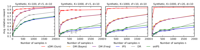
Figure 1: The relative reward of the learned policy on synthetic problems with varying $n$, $K$ and $d^{\prime}$.

6 Experiments

We evaluate sDM using both synthetic and MovieLens datasets. We use the average reward relative to the optimal policy as our evaluation metric, which is equivalent to the BSO. To match our theory, we consider linear rewards $\mathcal{N}(x^{\top}\theta_{*,a},1)$ for any action $a$ and context $x$. We provide supplementary experiments and details in Appendix F.

6.1 Synthetic Problems

We simulate synthetic data using the model in (15). The contexts $X$ are generated through uniform sampling from the range $[-1,1]^{d}$. Specifically, we choose a context dimension of $d=10$. The mixing matrices $\mathrm{W}_{a}$ are randomly drawn from $[-1,1]^{d\times d^{\prime}}$, where the latent dimension $d^{\prime}$ varies as $d^{\prime}\in\{5,10,20\}$. Additionally, we set the latent covariance as $\Sigma=3I_{d^{\prime}}$ and the conditional action covariances as $\Sigma_{a}=I_{d}$. This choice of covariances is because sDM is more beneficial when the latent parameters are more uncertain than the action parameters. Finally, the latent mean $\mu$ is randomly sampled from $[-1,1]^{d^{\prime}}$. The number of actions varies as $K\in\{10^{2},10^{3}\}$. We use a uniform logging policy to collect data while we defer the results with $\epsilon$-greedy logging policies to Appendix F.

We evaluate several baseline methods in our experiments. First, we consider the performance of sDM under a linear hierarchy with linear rewards in (15). Second, we examine DM (Bayes), which involves marginalizing out the latent parameters $\psi$ in (15). Our baselines also include DM (Freq), which estimates $\theta_{*,a}$ using the MLE. We further include IPS (Horvitz & Thompson, 1952), self-normalized IPS (snIPS) (Swaminathan & Joachims, 2015b), DR (Dudik et al., 2014), and these estimators are optimized directly without any regularization. This is because the goal of these experiments is not to compare with IPS and its variants. In particular, note that this experimental setting is better suited for DMs due to its high number of actions, known reward function, and well-specified priors, which is expected to favor DMs over IPS variants. Nevertheless, we include the IPS variants for the sake of completeness.

In Figure 1, we plot the average relative reward for the synthetic problems with varying sample size $n$. Overall, sDM consistently outperforms the baselines in terms of both sample efficiency and average reward. This performance gap becomes even more significant when dealing with scenarios featuring a high number of actions $K$, a limited sample size $n$, or suboptimal logging policies like uniform sampling. These results emphasize the enhanced efficiency of sDM in using the available logged data, making it particularly beneficial in data-limited situations and scalable to large action spaces. Also, the performance of sDM is still good even when $d^{\prime}>d$. In fact, its performance only deteriorates when $d^{\prime}\approx dK$, and hence the performance is still valid for larger $d^{\prime}$ as long as they are not in the order of $dK$. This highlights the significance of leveraging action correlations and latent structure as a robust approach for scaling OPL to practical scenarios while enjoying theoretical guarantees.

Large action spaces. sDM achieves improved scalability, in the sense that its performance remains robust in large action spaces, by leveraging data more efficiently. While it still learns a $d$-dim. parameter for each action $a$, it does so by considering interactions with all actions in the sample set $S$, instead of only using interactions with the specific action $a$. This is crucial, especially given that many actions may not even be observed in $S$. To show sDM’s improved scalability, we compared it to the most competitive baseline, DM (Bayes), for varying $K\in[10,10^{5}]$ with $n=10^{3}$. The results in Figure 2 reveal that the performance gap between sDM and DM (Bayes) becomes more significant when the number of actions $K$ increases. Hence, despite the necessity for sDM to learn distinct parameters for each action, accommodating practical scenarios like recommender systems where unique embeddings are learned for each product, it still enjoys good scalability to large action spaces.

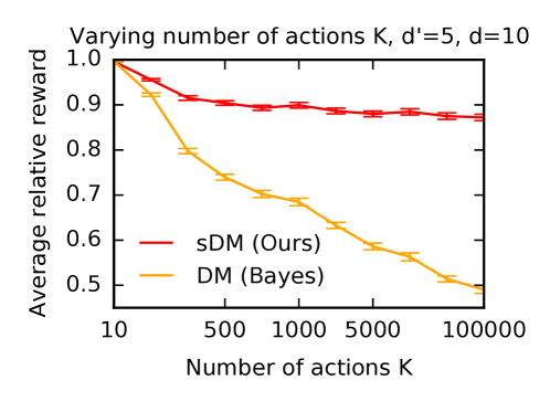
Figure 2: The average relative reward of sDM and DM (Bayes) with varying number of actions.

6.2 MovieLens Problems

Similar to Hong et al. (2023), we assess the performance of our baselines using the MovieLens 1M dataset (Lam & Herlocker, 2016). This dataset contains 1M ratings, reflecting the interactions of a set of 6,040 users with a collection of 3,952 movies. Our evaluation approach involves the creation of a semi-synthetic environment as follows. Initially, we apply a low-rank factorization technique to the rating matrix, yielding 5-dimensional representations denoted as $x_{u}\in^{5}$ for user $u\in[6040]$ and $\theta_{a}\in^{5}$ for movie $a\in[3952]$. Subsequently, the movies are treated as actions, and the contexts $X$ are sampled randomly from the user vectors. The reward associated with movie $a$ for user $u$ is modeled as $\mathcal{N}(x_{u}^{\top}\theta_{a},1)$, effectively representing a proxy for the rating. We employ a uniform logging policy to generate logged data, while additional experiments with an $\epsilon$-greedy logging policy can be found in Appendix F.

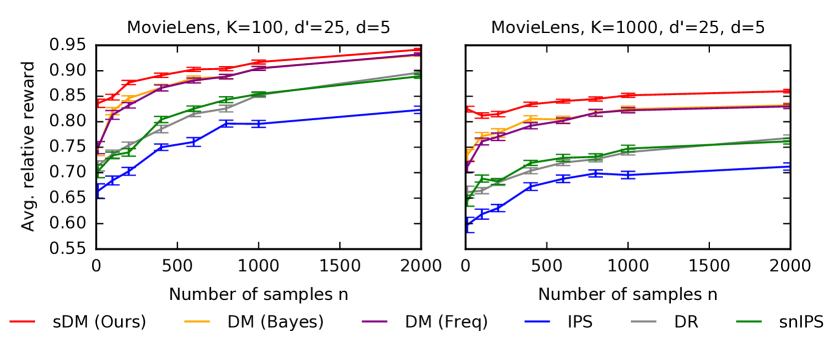
Figure 3: The average relative reward of the learned policy on MovieLens with varying $n$ and $K$.

A prior is not needed for DM (Freq), IPS, snIPS, and DR. However, for DM (Bayes), a prior is inferred from data, where we set $\mu_{a}$ to be the mean of movie vectors across all dimensions, and $\Sigma_{a}={\rm diag}(v)$, where $v$ represents the variance of movie vectors across all dimensions. Note that, unlike the synthetic experiments, the latent structure assumed by sDM is not inherently present in the MovieLens dataset. Nevertheless, we learn it by training a Gaussian Mixture Model (GMM) to cluster movies into $J=5$ mixture components. This gives rise to the mixed-effect structure described in Section 4, which represents a specific instance of sDM with $d^{\prime}=dJ=25$. Both DM (Bayes) and sDM use the same subset of data to learn their priors and it is of size $\{100,1000\}$ depending on the setting. We conduct two experiments with $K\in\{10^{2},10^{3}\}$ randomly selected movies, and the results are in Figure 3. Even though the latent structure assumed by sDM is absent, sDM still outperforms the baselines.

7 Conclusion

We introduced sDM, a novel approach for OPE and OPL with large action spaces. sDM leverages latent structures among actions to enhance statistical efficiency while preserving computational efficiency. Our experiments validate our theory. Notably, when employing Bayesian metrics like the BSO, the benefits of using informative and structured priors become prominent, particularly in large action spaces with limited data. However, we acknowledge the primary limitation of our work, which is the assumption of well-specified priors. Consequently, exploring methods to relax this assumption represents a promising avenue for future research. Furthermore, extending the applicability of sDM to non-linear hierarchies is also important.

Broader Impact

This work contributes to the development and analysis of practical algorithms for offline learning to act under uncertainty. While our generic setting and algorithms have broad potential applications, the specific downstream social impacts are inherently dependent on the chosen application.

Organization of the Supplementary Material

The supplementary material is organized as follows.

• In Appendix A, we provide a detailed notation.

• In Appendix B, we provide an extended related work discussion.

• In Appendix C, we outline the posterior derivations for the standard prior in (3).

• Transitioning to Appendix D, we outline the posterior derivations under the structured priors in (15).

• In Appendix E, we prove the claims made in Section 5.

• Finally, in Appendix F, we present supplementary experiments.

Appendix A Detailed Notation

For any positive integer $n$, we define $[n]$ as the set ${1,2,\ldots,n}$. We represent the identity matrix of dimension $d\times d$ as $I_{d}$. In our notation, unless explicitly stated otherwise, the $i$-th coordinate of a vector $v$ is denoted as $v_{i}$. However, if the vector is already indexed, such as $x_{i}$, we use the notation $x_{i,j}$ to represent the $j$-th entry of the vector $x_{i}$. When dealing with matrices, we refer to the $(i,j)$-th entry of a matrix $\mathrm{A}$ as $\mathrm{A}_{i,j}$. Also, $\lambda_{1}(\mathrm{A})$ and $\lambda_{d}(\mathrm{A})$ refer to the maximum and minimum eigenvalues of matrix $\mathrm{A}$, respectively. Moreover, for any positive-definite matrix $A$ and vector $x$, we let $\|x\|_{A}=\sqrt{x^{\top}Ax}$.

Now, consider a collection of $n$ vectors, denoted as $a_{1}\in^{d},a_{2}\in^{d},\ldots,a_{n}\in^{d}$. Then we use $a=(a_{i})_{i\in[n]}\in\mathbb{R}^{nd}$ to represent a $nd$-dimensional vector formed by concatenating the vectors $a_{1},a_{2},\ldots,a_{n}$. The operator $\operatorname{Vec}(\cdot)$ is used to vectorize a matrix or a set of vectors. Let $\mathrm{A}_{1},\mathrm{A}_{2},\ldots,\mathrm{A}_{n}$ be a collection of $n$ matrices, each of dimension $d\times d$. The notation $\mathrm{diag}((\mathrm{A}_{i})_{i\in[n]})\in^{nd\times nd}$ represents a block diagonal matrix where $\mathrm{A}_{1},\mathrm{A}_{2},\ldots,\mathrm{A}_{n}$ are the main-diagonal blocks. Similarly, $(\mathrm{A}_{i})_{i\in[n]}\in^{nd\times d}$ denotes the $nd\times d$ matrix formed by concatenating matrices $\mathrm{A}_{1},\mathrm{A}_{2},\ldots,\mathrm{A}_{n}$. To provide a more visual representation, consider a collection of vectors $a_{1}\in^{d},a_{2}\in^{d},\ldots,a_{n}\in^{d}$ and matrices $\mathrm{A}_{1}\in^{d\times d},\mathrm{A}_{2}\in^{d\times d},\ldots,\mathrm{A}_{n}\in^{d\times d}$. We can represent them as follows

$$(a_{i})_{i\in[n]}={\begin{pmatrix}a_{1}\\ a_{2}\\ \vdots\\ a_{n}\end{pmatrix}}\in^{nd}\,,\quad\mathrm{diag}((\mathrm{A}_{i})_{i\in[n]})={\begin{pmatrix}\mathrm{A}_{1}&0&\cdots&0\\ 0&\mathrm{A}_{2}&\cdots&0\\ \vdots&\vdots&\ddots&\vdots\\ 0&0&\cdots&\mathrm{A}_{n}\end{pmatrix}}\in^{nd\times nd}\,,\quad(\mathrm{A}_{i})_{i\in[n]}={\begin{pmatrix}\mathrm{A}_{1}\\ \mathrm{A}_{2}\\ \vdots\\ \mathrm{A}_{n}\end{pmatrix}}\in^{nd\times d}\,.$$

Appendix B Extended Related Work

Online learning under uncertainty is often modeled within the framework of contextual bandits (Lattimore & Szepesvari, 2019; Li et al., 2010; Chu et al., 2011). Naturally, learning within this framework follows an online paradigm. However, practical applications often entail a large action space and a significant emphasis on short-term gains. This presents a challenge where the agent needs to exhibit a risk-averse behavior, contradicting the foundational principle of online algorithms designed to explore actions for long-term benefit (Auer et al., 2002; Thompson, 1933; Russo et al., 2018; Agrawal & Goyal, 2013; Abbasi-Yadkori et al., 2011). While several practical online algorithms have emerged to efficiently explore the action space in contextual bandits (Zong et al., 2016; Zhu et al., 2022; Aouali et al., 2023b; Aouali, 2023), a notable gap exists in the quest for an offline procedure capable of optimizing decision-making using historical data. Fortunately, we are often equipped with a sample set collected from past interactions. Leveraging this data, agents can enhance their policies offline (Swaminathan & Joachims, 2015a; London & Sandler, 2019; Sakhi et al., 2022), consequently improving the overall system performance. This study is primarily concerned with this offline or off-policy formulation of contextual bandits (Dudík et al., 2011, 2012; Dudik et al., 2014; Wang et al., 2017; Farajtabar et al., 2018). There are two main tasks in off-policy contextual bandits, first, off-policy evaluation (OPE) (Dudík et al., 2011) which involves estimating policy performance using historical data, simulating as if these evaluations were performed while the policy is interacting with the environment in real-time. Subsequently, the derived estimator is refined to closely approximate the optimal policy, a process known as off-policy learning (OPL) (Swaminathan & Joachims, 2015a). Next, we review both OPE and OPL.

B.1 Off-Policy Evaluation

Recent years have witnessed a surge in interest in OPE, with several key works contributing to this field (Dudík et al., 2011, 2012; Dudik et al., 2014; Wang et al., 2017; Farajtabar et al., 2018; Su et al., 2019, 2020; Metelli et al., 2021; Kuzborskij et al., 2021; Saito & Joachims, 2022; Sakhi et al., 2020; Jeunen & Goethals, 2021). The literature on OPE can be broadly categorized into three main approaches. The first approach referred to as the direct method (DM) (Jeunen & Goethals, 2021; Hong et al., 2023), involves learning a model that approximates the expected reward. This model is then used to estimate the performance of evaluated policies. The second approach, inverse propensity scoring (IPS) (Horvitz & Thompson, 1952; Dudík et al., 2012), aims to estimate the reward of evaluated policies by correcting for the preference bias of the logging policy in the sample set. IPS is unbiased when there’s an assumption that the evaluation policy is absolutely continuous with respect to the logging policy. However, it can exhibit high variance and substantial bias when this assumption is violated (Sachdeva et al., 2020). Various techniques have been introduced to address the variance issue, such as clipping importance weights (Ionides, 2008; Swaminathan & Joachims, 2015a), smoothing them (Aouali et al., 2023a), self-normalization of weights (Swaminathan & Joachims, 2015b), etc. (Gilotte et al., 2018). The third approach, known as doubly robust (DR) (Robins & Rotnitzky, 1995; Bang & Robins, 2005; Dudík et al., 2011; Dudik et al., 2014; Farajtabar et al., 2018), combines elements of DM and IPS, helping to reduce variance. Assessing the accuracy of an OPE estimator, denoted as $\hat{R}_{n}(\pi)$, is typically done using the mean squared error (MSE). It may be relevant to note that Metelli et al. (2021) argued that high-probability concentration rates should be preferred over the MSE to evaluate OPE estimators as they provide non-asymptotic guarantees. In this work, we presented a direct method for OPE, for which we could derive both an MSE and high-probability concentration bound under our assumptions. However, we focused more on OPL.

B.2 Off-Policy Learning

OPL under IPS. Prior research on OPL predominantly revolved around developing learning principles influenced by generalization bounds for IPS. Swaminathan & Joachims (2015a) proposed to penalize the IPS estimator with a variance term leading to a learning principle that promotes policies that achieve high estimated reward and exhibit minimal empirical variance. In a recent development, London et al. (London & Sandler, 2019) made a connection between PAC-Bayes theory and OPL that inspired several works in the same vein (Sakhi et al., 2022; Aouali et al., 2023a). London & Sandler (2019) proposed a learning principle that favors policies with high estimated reward while keeping the parameter close to that of the logging policy in terms of $L_{2}$ distance. In particular, this learning principle is scalable. Then Sakhi et al. (2022); Aouali et al. (2023a) took a different direction of deriving tractable generalization bounds and optimizing them directly as they are. Finally, Wang et al. (2023) recently introduced an efficient learning principle with guarantees for a specific choice of their hyperparameter. All of these learning principles are related to the concept of pessimism which we discuss next.

OPL under DM. The majority of OPL approaches in contextual bandits rely on the principle of pessimism (Jeunen & Goethals, 2021; Jin et al., 2021; Hong et al., 2023). In essence, these methods construct confidence intervals for reward estimates $\hat{r}(x,a),$ that hold simultaneously for all $(x,a)\in\mathcal{X}\times\mathcal{A}$ and satisfy the following condition

$$|r(x,a;\theta)-\hat{r}(x,a)| \leq u(x,a)\,, \forall(x,a)\in\mathcal{X}\times\mathcal{A}$$

Subsequently, the policy learned with this pessimistic approach is defined as

$$\hat{\pi}_{\textsc{p}}(a\mid x)=\mathds{1}_{\{a=\operatorname*{argmax}_{b\in\mathcal{A}}\hat{r}(x,b)-u(x,b)\}}\,.$$ (26)

Note that when the function $u(x,a)$ is independent of both $x$ and $a$, the pessimistic and greedy policies become equivalent. However, in this work, we highlight the critical role of the selected metric and the underlying assumptions about $\hat{r}$ in choosing between pessimistic and greedy policies. In particular, we introduce the concept of Bayesian suboptimality (BSO), as defined in Section 5.1. BSO evaluates the average performance of algorithms across multiple problem instances, and in this context, the Greedy policy emerges as a more suitable choice for minimizing the BSO. A detailed comparison of pessimistic and greedy policies is presented in Section E.4.

In addition to not using pessimism, our work also considers structured contextual bandit problems, upon which we build informative priors. Notably, while structured problems have been previously investigated in the context of multi-task learning by Lazaric & Ghavamzadeh (2010); Hong et al. (2023), these works primarily focused on cases where there are multiple contextual bandit instances that bear similarity to one another. Interaction with one bandit instance contributes to the agent’s understanding of other instances. In contrast, our work tackles a single contextual bandit instance with a large action space and considers an inherent structure among actions within this bandit instance. Furthermore, the structure we address in the single-instance problem is different and more general compared to the ones explored in the aforementioned multi-task learning works.

Appendix C Posterior Derivations Under Standard Priors

Here we derive the posterior under the standard prior in (3). These are standard derivations and we present them here for the sake of completeness.

Derivation of $\,p(\theta_{a}\mid S)$ for the standard prior in (3).

We start by recalling the standard prior in (3)

$$\theta_{a} \sim\mathcal{N}(\mu_{a},\Sigma_{a})\,, \forall a\in\mathcal{A}\,,$$ (27)

$$R\mid\theta,X,A \sim\mathcal{N}(\phi(X)^{\top}\theta_{A},\sigma^{2})\,,$$

where $\mathcal{N}(\mu_{a},\Sigma_{a})$ is the prior on the action parameter $\theta_{a}$. Let $\theta=(\theta_{a})_{a\in\mathcal{A}}\in^{dK}$, $\Sigma_{\mathcal{A}}={\rm diag}(\Sigma_{a})_{a\in\mathcal{A}}\in^{dK\times dK}$ and $\mu_{\mathcal{A}}=(\mu_{a})_{a\in\mathcal{A}}\in^{dK}$. Also, let $u_{a}\in\left\{0,1\right\}^{K}$ be the binary vector representing the action $a$. That is, $u_{a,a}=1$ and $u_{a,a^{\prime}}=0$ for all $a^{\prime}\neq a$. Then we can rewrite the model in (27) as

$$\theta \sim\mathcal{N}(\mu_{\mathcal{A}},\Sigma_{\mathcal{A}})\,,$$ (28)

$$R\mid\theta,X,A \sim\mathcal{N}((u_{A}\otimes\phi(X))^{\top}\theta,\sigma^{2})\,.$$

Then the joint action posterior $p(\theta\mid S)$ decomposes as

$$p( \theta\mid S)=p(\theta\mid(X_{i},A_{i},R_{i})_{i\in[n]})\stackrel{{\scriptstyle(i)}}{{\propto}}p((R_{i})_{i\in[n]}\mid\theta,(X_{i},A_{i})_{i\in[n]})p(\theta\mid(X_{i},A_{i})_{i\in[n]})\,,$$

$$\stackrel{{\scriptstyle(ii)}}{{=}}p((R_{i})_{i\in[n]}\mid\theta,(X_{i},A_{i})_{i\in[n]})p(\theta)\stackrel{{\scriptstyle(iii)}}{{=}}\prod_{i\in[n]}p(R_{i}\mid\theta,X_{i},A_{i})p(\theta)\,,$$

$$\stackrel{{\scriptstyle(iv)}}{{=}}\prod_{i\in[n]}\mathcal{N}(R_{i};(u_{A_{i}}\otimes\phi(X_{i}))^{\top}\theta,\sigma^{2})\mathcal{N}(\theta;\mu_{\mathcal{A}},\Sigma_{\mathcal{A}})\,,$$

$$=\exp\left[-\frac{1}{2}\left(v\sum_{i=1}^{n}(R_{i}^{2}-2R_{i}(u_{A_{i}}\otimes\phi(X_{i}))^{\top}\theta+((u_{A_{i}}\otimes\phi(X_{i}))^{\top}\theta)^{2})+\theta^{\top}\Lambda_{\mathcal{A}}\theta-2\theta^{\top}\Lambda_{\mathcal{A}}\mu_{\mathcal{A}}+\mu_{\mathcal{A}}^{\top}\Lambda_{\mathcal{A}}\mu_{\mathcal{A}}\right)\right]\,,$$

$$\propto\exp\left[-\frac{1}{2}\left(\theta^{\top}(v\sum_{i=1}^{n}(u_{A_{i}}\otimes\phi(X_{i}))(u_{A_{i}}\otimes\phi(X_{i}))^{\top}+\Lambda_{\mathcal{A}})\theta-2\theta^{\top}\left(v\sum_{i=1}^{n}(u_{A_{i}}\otimes\phi(X_{i}))^{\top}R_{i}+\Lambda_{\mathcal{A}}\mu_{\mathcal{A}}\right)\right)\right]\,,$$

$$=\exp\left[-\frac{1}{2}\left(\theta^{\top}(v\sum_{i=1}^{n}(u_{A_{i}}u_{A_{i}}^{\top}\otimes\phi(X_{i})\phi(X_{i})^{\top})+\Lambda_{\mathcal{A}})\theta-2\theta^{\top}\left(v\sum_{i=1}^{n}(u_{A_{i}}\otimes\phi(X_{i}))^{\top}R_{i}+\Lambda_{\mathcal{A}}\mu_{\mathcal{A}}\right)\right)\right]\,,$$

$$\stackrel{{\scriptstyle(v)}}{{\propto}}\mathcal{N}\left(\theta;\hat{\mu}_{\mathcal{A}},\left(\hat{\Lambda}_{\mathcal{A}}\right)^{-1}\right)\,.$$

In $(i)$, we apply Bayes rule. In $(ii)$, we use that $\theta$ is independent of $(X,A)$, and $(iii)$ follows from the assumption that $R_{i}\mid\theta,X_{i},A_{i}$ are i.i.d. Finally, in $(iv)$, we replace the distribution by their Gaussian form, and in $(v)$, we set $\hat{\Lambda}_{\mathcal{A}}=v\sum_{i=1}^{n}(u_{A_{i}}u_{A_{i}}^{\top}\otimes\phi(X_{i})\phi(X_{i})^{\top})+\Lambda_{\mathcal{A}}\,,$ and $\hat{\mu}_{a}=\hat{\Lambda}_{\mathcal{A}}^{-1}\big{(}v\sum_{i=1}^{n}(u_{A_{i}}\otimes\phi(X_{i}))^{\top}R_{i}+\Lambda_{\mathcal{A}}\mu_{\mathcal{A}}\Big{)}$. Now notice that $\hat{\Lambda}_{\mathcal{A}}={\rm diag}(\Sigma_{a}^{-1}+G_{a})_{a\in\mathcal{A}}$. Thus, $p(\theta\mid S)=\mathcal{N}(\theta,\hat{\mu}_{\mathcal{A}},\Lambda_{\mathcal{A}}^{-1})$ where $\hat{\mu}_{\mathcal{A}}=(\hat{\mu}_{a})_{a\in\mathcal{A}}$ and $\Lambda_{\mathcal{A}}={\rm diag}(\hat{\Lambda}_{a})_{a\in\mathcal{A}}\,,$ with

$$\hat{\Lambda}_{a}=\Sigma_{a}^{-1}+G_{a}\,, \hat{\Lambda}_{a}\hat{\mu}_{a} =\Sigma_{a}^{-1}\mu_{a}+B_{a}\,.$$

Since the covariance matrix of $p(\theta\mid S)$ is diagonal by block, we know that the marginals $\theta_{a}\mid S$ also have a Gaussian density $p(\theta_{a}\mid S)=\mathcal{N}(\theta_{a};\hat{\mu}_{a},\hat{\Sigma}_{a})$ where $\hat{\Sigma}_{a}=\hat{\Lambda}_{a}^{-1}$.

∎

Appendix D Posterior Derivations Under Structured Priors

Here we derive the posteriors under the structured prior in (15). Precisely, we derive the latent posterior density of $\psi\mid S$, the conditional posterior density of $\theta\mid S,\psi$. Then, we derive the marginal posterior $\theta\mid S$.

D.1 Latent Posterior

Derivation of $\,p(\psi\mid S)$.

First, recall that our model in (15) reads

$$\psi \sim\mathcal{N}(\mu,\Sigma)\,,$$

$$\theta_{a}\mid\psi \sim\mathcal{N}\Big{(}\mathrm{W}_{a}\psi,\,\Sigma_{a}\Big{)}\,, \forall a\in\mathcal{A}\,,$$

$$R\mid\psi,\theta,X,A \sim\mathcal{N}(\phi(X)^{\top}\theta_{A},\sigma^{2})\,.$$ (29)

Then we first rewrite it as

$$\psi \sim\mathcal{N}(\mu,\Sigma)\,,$$

$$\theta\mid\psi \sim\mathcal{N}\Big{(}\mathrm{W}_{\mathcal{A}}\psi,\,\Sigma_{\mathcal{A}}\Big{)}\,,$$

$$R\mid\psi,\theta,X,A \sim\mathcal{N}((u_{A}\otimes\phi(X))^{\top}\theta,\sigma^{2})\,.$$ (30)

Then the latent posterior is

$$p(\psi\mid(X_{i},A_{i},R_{i})_{i\in[n]}) \propto p((R_{i})_{i\in[n]}\mid\psi,(X_{i},A_{i})_{i\in[n]})p(\psi\mid(X_{i},A_{i})_{i\in[n]})\,,$$

$$\stackrel{{\scriptstyle(i)}}{{=}}p((R_{i})_{i\in[n]}\mid\psi,(X_{i},A_{i})_{i\in[n]})q(\psi)\,,$$

$$=\int_{\theta}p((R_{i})_{i\in[n]},\theta\mid\psi,(X_{i},A_{i})_{i\in[n]})\mathop{}\!\mathrm{d}\theta\,q(\psi)\,,$$

$$=\int_{\theta}p((R_{i})_{i\in[n]}\mid\psi,\theta,(X_{i},A_{i})_{i\in[n]})p(\theta\mid\psi,(X_{i},A_{i})_{i\in[n]})\mathop{}\!\mathrm{d}\theta\,q(\psi)\,,$$

$$\stackrel{{\scriptstyle(ii)}}{{=}}\int_{\theta}p((R_{i})_{i\in[n]}\mid\psi,\theta,(X_{i},A_{i})_{i\in[n]})p(\theta\mid\psi)\mathop{}\!\mathrm{d}\theta\,q(\psi)\,,$$

In $(i)$, we use that $(X,A)$ is independent of $\psi$, which follows from 3.2. Similarly, in $(ii)$, we use that $\theta$ is conditionally independent of $(X,A)$ given $\psi$. Now we know that given $\theta$, $R_{i}\mid X_{i},A_{i}$ are i.i.d. and hence $p((R_{i})_{i\in[n]}\mid\psi,\theta,(X_{i},A_{i})_{i\in[n]})=\prod_{a\in\mathcal{A}}\mathcal{L}_{a}(\theta_{a})$. Moreover, $\theta_{a}$ for $a\in\mathcal{A}$ are conditionally independent given $\psi$. Thus $p(\theta\mid\psi)=\prod_{a\in\mathcal{A}}p_{a}\left(\theta_{a};f_{a}(\psi)\right)$, where we also used that $\theta_{a}\mid\psi\sim p_{a}\left(\cdot;f_{a}(\psi)\right)$. This leads to

$$p(\psi\mid(X_{i},A_{i},R_{i})_{i\in[n]}) \propto\int_{\theta}\prod_{a\in\mathcal{A}}\mathcal{L}_{a}(\theta_{a})p_{a}\left(\theta_{a};f_{a}(\psi)\right)\mathop{}\!\mathrm{d}\theta\,q(\psi)\,,$$

$$\stackrel{{\scriptstyle(i)}}{{=}}\prod_{a\in\mathcal{A}}\int_{\theta_{a}}\mathcal{L}_{a}(\theta_{a})\mathcal{N}\left(\theta_{a};\mathrm{W}_{a}\psi,\Sigma_{a}\right)\mathop{}\!\mathrm{d}\theta_{a}\mathcal{N}(\psi;\mu,\Sigma)\,,$$

$$\stackrel{{\scriptstyle(ii)}}{{=}}\prod_{a\in\mathcal{A}}\int_{\theta_{a}}\Big{(}\prod_{i\in I_{a}}\mathcal{N}(R_{i};\phi(X_{i})^{\top}\theta_{a},\sigma^{2})\Big{)}\mathcal{N}\left(\theta_{a};\mathrm{W}_{a}\psi,\Sigma_{a}\right)\mathop{}\!\mathrm{d}\theta_{a}\mathcal{N}(\psi;\mu,\Sigma)\,.$$

In $(i)$, we notice that $\theta=(\theta_{a})_{a\in\mathcal{A}}$ and apply Fubini’s Theorem. In $(ii)$, we let $I_{a}=|S_{a}|=\sum_{i\in[n]}\mathds{1}_{\{A_{i}=a\}}$ as the number of times action $a$ appears in the sample set $S$. Now let $h_{a}(\psi)=\int_{\theta_{a}}\left(\prod_{i\in I_{a}}\mathcal{N}(R_{i};\phi(X_{i})^{\top}\theta_{a},\sigma^{2})\right)\mathcal{N}\left(\theta_{a};\mathrm{W}_{a}\psi,\Sigma_{a}\right)\mathop{}\!\mathrm{d}\theta$. Then we have that

$$p(\psi\mid S) \propto\prod_{a\in\mathcal{A}}h_{a}(\psi)\mathcal{N}(\psi;\mu,\Sigma)\,.$$ (31)

We start by computing $h_{a}$. To reduce clutter, let $v=\sigma^{-2}$ and $\Lambda_{a}=\Sigma_{a}^{-1}$. Then we compute $h_{a}$ as

$$h_{a}(\psi)=\int_{\theta_{a}}\left(\prod_{i\in I_{a}}\mathcal{N}(R_{i};\phi(X_{i})^{\top}\theta_{a},\sigma^{2})\right)\mathcal{N}(\theta_{a};\mathrm{W}_{a}\psi,\Sigma_{a})\mathop{}\!\mathrm{d}\theta_{a}\,,$$

$$\propto\int_{\theta_{a}}\exp\left[-\frac{1}{2}v\sum_{i\in I_{a}}(R_{i}-\phi(X_{i})^{\top}\theta_{a})^{2}-\frac{1}{2}(\theta_{a}-\mathrm{W}_{a}\psi)^{\top}\Lambda_{a}(\theta_{a}-\mathrm{W}_{a}\psi)\right]\mathop{}\!\mathrm{d}\theta_{a}\,,$$

$$=\int_{\theta_{a}}\exp\Big{[}-\frac{1}{2}\Big{(}v\sum_{i\in I_{a}}(R_{i}^{2}-2R_{i}\theta_{a}^{\top}\phi(X_{i})+(\theta_{a}^{\top}\phi(X_{i}))^{2})+\theta_{a}^{\top}\Lambda_{a}\theta_{a}-2\theta_{a}^{\top}\Lambda_{a}\mathrm{W}_{a}\psi$$

$$\hskip 341.43306pt+(\mathrm{W}_{a}\psi)^{\top}\Lambda_{a}(\mathrm{W}_{a}\psi)\Big{)}\Big{]}\mathop{}\!\mathrm{d}\theta_{a}\,,$$

$$\propto\int_{\theta_{a}}\exp\Big{[}-\frac{1}{2}\Big{(}\theta_{a}^{\top}\left(v\sum_{i\in I_{a}}\phi(X_{i})\phi(X_{i})^{\top}+\Lambda_{a}\right)\theta_{a}-2\theta_{a}^{\top}\left(v\sum_{i\in I_{a}}R_{i}\phi(X_{i})+\Lambda_{a}\mathrm{W}_{a}\psi\right)$$

$$\hskip 341.43306pt+(\mathrm{W}_{a}\psi)^{\top}\Lambda_{a}(\mathrm{W}_{a}\psi)\Big{)}\Big{]}\mathop{}\!\mathrm{d}\theta_{a}\,.$$

Now recall that $G_{a}=v\sum_{i\in I_{a}}\phi(X_{i})\phi(X_{i})^{\top}$ and $B_{a}=v\sum_{i\in I_{a}}R_{i}\phi(X_{i})$ and let $V_{a}=\left(G_{a}+\Lambda_{a}\right)^{-1}$, $U_{a}=V_{a}^{-1}$, and $\beta_{a}=V_{a}(B_{a}+\Lambda_{a}\mathrm{W}_{a}\psi)$. Then have that $U_{a}V_{a}=V_{a}U_{a}=I_{d}\,,$ and thus

$$f(\psi) \propto\int_{\theta_{a}}\exp\left[-\frac{1}{2}\left(\theta_{a}^{\top}U_{a}\theta_{a}-2\theta_{a}^{\top}U_{a}V_{a}\left(B_{a}+\Lambda_{a}\mathrm{W}_{a}\psi\right)+(\mathrm{W}_{a}\psi)^{\top}\Lambda_{a}(\mathrm{W}_{a}\psi)\right)\right]\mathop{}\!\mathrm{d}\theta_{a}\,,$$

$$=\int_{\theta_{a}}\exp\left[-\frac{1}{2}\left(\theta_{a}^{\top}U_{a}\theta_{a}-2\theta_{a}^{\top}U_{a}\beta_{a}+(\mathrm{W}_{a}\psi)^{\top}\Lambda_{a}(\mathrm{W}_{a}\psi)\right)\right]\mathop{}\!\mathrm{d}\theta_{a}\,,$$

$$=\int_{\theta_{a}}\exp\left[-\frac{1}{2}\left((\theta_{a}-\beta_{a})^{\top}U_{a}(\theta_{a}-\beta_{a})-\beta_{a}^{\top}U_{a}\beta_{a}+(\mathrm{W}_{a}\psi)^{\top}\Lambda_{a}(\mathrm{W}_{a}\psi)\right)\right]\mathop{}\!\mathrm{d}\theta_{a}\,,$$

$$\propto\exp\left[-\frac{1}{2}\left(-\beta_{a}^{\top}U_{a}\beta_{a}+(\mathrm{W}_{a}\psi)^{\top}\Lambda_{a}(\mathrm{W}_{a}\psi)\right)\right]\,,$$

$$=\exp\left[-\frac{1}{2}\left(-\left(B_{a}+\Lambda_{a}\mathrm{W}_{a}\psi\right)^{\top}V_{a}\left(B_{a}+\Lambda_{a}\mathrm{W}_{a}\psi\right)+(\mathrm{W}_{a}\psi)^{\top}\Lambda_{a}(\mathrm{W}_{a}\psi)\right)\right]\,,$$

$$\propto\exp\left[-\frac{1}{2}\left(\psi^{\top}\mathrm{W}_{a}^{\top}\left(\Lambda_{a}-\Lambda_{a}V_{a}\Lambda_{a}\right)\mathrm{W}_{a}\psi-2\psi^{\top}\left(\mathrm{W}_{a}^{\top}\Lambda_{a}V_{a}B_{a}\right)\right)\right]\,,$$

$$\propto\mathcal{N}(\psi;\bar{\mu}_{a},\bar{\Sigma}_{a})\,,$$

where

$$\bar{\Sigma}_{a}^{-1} =\mathrm{W}_{a}^{\top}\left(\Lambda_{a}-\Lambda_{a}V_{a}\Lambda_{a}\right)\mathrm{W}_{a}=\mathrm{W}_{a}^{\top}\left(\Sigma_{a}^{-1}-\Sigma_{a}^{-1}(G_{a}+\Sigma_{a}^{-1})^{-1}\Sigma_{a}^{-1}\right)\mathrm{W}_{a}\,,$$

$$\bar{\Sigma}_{a}^{-1}\bar{\mu}_{a} =\mathrm{W}_{a}^{\top}\Lambda_{a}V_{a}B_{a}=\mathrm{W}_{a}^{\top}\Sigma_{a}^{-1}(G_{a}+\Sigma_{a}^{-1})^{-1}B_{a}\,.$$ (32)

However, we know from (31) that $p(\psi\mid S)\propto\prod_{a\in\mathcal{A}}h_{a}(\psi)\mathcal{N}(\psi;\mu,\Sigma)$. But $h_{a}(\psi)$ is proportional to $\mathcal{N}(\psi;\bar{\mu}_{a},\bar{\Sigma}_{a})$ for any $a$. Thus $p(\psi\mid S)$ can be seen as the product of $K+1$ multivariate Gaussian distributions $\mathcal{N}(\mu,\Sigma)$ and $\mathcal{N}(\bar{\mu}_{a},\bar{\Sigma}_{a})$ for $a\in\mathcal{A}$ (the terms $h_{a}$). Thus, $p(\psi\mid S)$ is also a multivariate Gaussian distribution $\mathcal{N}(\bar{\mu},\bar{\Sigma}^{-1})$, with

$$\bar{\Sigma}^{-1} =\Sigma^{-1}+\sum_{a\in\mathcal{A}}\bar{\Sigma}_{a}^{-1}=\Sigma^{-1}+\sum_{a\in\mathcal{A}}\mathrm{W}_{a}^{\top}\left(\Sigma_{a}^{-1}-\Sigma_{a}^{-1}(G_{a}+\Sigma_{a}^{-1})^{-1}\Sigma_{a}^{-1}\right)\mathrm{W}_{a}\,,$$ (33)

$$\bar{\Sigma}^{-1}\bar{\mu} =\Sigma^{-1}\mu+\sum_{a\in\mathcal{A}}\bar{\Sigma}_{a}^{-1}\bar{\mu}_{a}=\Sigma^{-1}\mu+\sum_{a\in\mathcal{A}}\mathrm{W}_{a}^{\top}\Sigma_{a}^{-1}(G_{a}+\Sigma_{a}^{-1})^{-1}B_{a}\,.$$ (34)

∎

D.2 Conditional Posterior

Derivation of $\,p(\theta_{a}\mid\psi,S)$.

Let $v=\sigma^{-2}\,,\quad\Lambda_{a}=\Sigma_{a}^{-1}\,.$ We consider the model rewritten in (D.1), then the joint action posterior $p(\theta\mid S)$ decomposes as

$$p(\theta\mid\psi,S)=p(\theta\mid\psi,(X_{i},A_{i},R_{i})_{i\in[n]})\stackrel{{\scriptstyle(i)}}{{\propto}}p((R_{i})_{i\in[n]}\mid\theta,\psi,(X_{i},A_{i})_{i\in[n]})p(\theta\mid\psi,(X_{i},A_{i})_{i\in[n]})\,,$$

$$\stackrel{{\scriptstyle(ii)}}{{=}}p((R_{i})_{i\in[n]}\mid\theta,(X_{i},A_{i})_{i\in[n]})p(\theta\mid\psi)\stackrel{{\scriptstyle(iii)}}{{=}}\prod_{i\in[n]}p(R_{i}\mid\theta,X_{i},A_{i})p(\theta\mid\psi)\,,$$

$$\stackrel{{\scriptstyle(iv)}}{{=}}\prod_{i\in[n]}\mathcal{N}(R_{i};(u_{A_{i}}\otimes\phi(X_{i}))^{\top}\theta,\sigma^{2})\mathcal{N}(\theta;\mathrm{W}_{\mathcal{A}}\psi,\Sigma_{\mathcal{A}})\,,$$

$$=\exp\Big{[}-\frac{1}{2}\Big{(}v\sum_{i=1}^{n}(R_{i}^{2}-2R_{i}(u_{A_{i}}\otimes\phi(X_{i}))^{\top}\theta+((u_{A_{i}}\otimes\phi(X_{i}))^{\top}\theta)^{2})+\theta^{\top}\Lambda_{\mathcal{A}}\theta-2\theta^{\top}\Lambda_{\mathcal{A}}\mathrm{W}_{\mathcal{A}}\psi$$

$$\hskip 369.88582pt+\psi^{\top}\mathrm{W}_{\mathcal{A}}^{\top}\Lambda_{\mathcal{A}}\mathrm{W}_{\mathcal{A}}\psi\Big{)}\Big{]}\,,$$

$$\propto\exp\left[-\frac{1}{2}\left(\theta^{\top}(v\sum_{i=1}^{n}(u_{A_{i}}\otimes\phi(X_{i}))(u_{A_{i}}\otimes\phi(X_{i}))^{\top}+\Lambda_{\mathcal{A}})\theta-2\theta^{\top}\left(v\sum_{i=1}^{n}(u_{A_{i}}\otimes\phi(X_{i}))^{\top}R_{i}+\Lambda_{\mathcal{A}}\mathrm{W}_{\mathcal{A}}\psi\right)\right)\right]\,,$$

$$=\exp\Big{[}-\frac{1}{2}\Big{(}\theta^{\top}(v\sum_{i=1}^{n}(u_{A_{i}}u_{A_{i}}^{\top}\otimes\phi(X_{i})\phi(X_{i})^{\top})+\Lambda_{\mathcal{A}})\theta-2\theta^{\top}\left(v\sum_{i=1}^{n}(u_{A_{i}}\otimes\phi(X_{i}))^{\top}R_{i}+\Lambda_{\mathcal{A}}\mathrm{W}_{\mathcal{A}}\psi\right)\Big{)}\Big{]}\,,$$

$$\stackrel{{\scriptstyle(v)}}{{\propto}}\mathcal{N}\left(\theta;\tilde{\mu}_{\mathcal{A}},\left(\tilde{\Lambda}_{\mathcal{A}}\right)^{-1}\right)\,,$$

where we use Bayes rule in $(i)$, $(ii)$ uses two assumptions. First, Given $\theta,X,A$, $R$ is independent of $\psi$. Second, given $\psi$, $\theta$ is independent of $(X,A)$. Moreover, $(iii)$ follows from the assumption that $R_{i}\mid\theta,X_{i},A_{i}$ are i.i.d. Finally, in $iv$, we replace the distribution by their Gaussian form, and in $(v)$, we set $\tilde{\Lambda}_{\mathcal{A}}=v\sum_{i=1}^{n}(u_{A_{i}}u_{A_{i}}^{\top}\otimes\phi(X_{i})\phi(X_{i})^{\top})+\Lambda_{\mathcal{A}}\,,$ and $\tilde{\mu}_{a}=\tilde{\Lambda}_{\mathcal{A}}^{-1}\big{(}v\sum_{i=1}^{n}(u_{A_{i}}\otimes\phi(X_{i}))^{\top}R_{i}+\Lambda_{\mathcal{A}}\mathrm{W}_{\mathcal{A}}\psi\Big{)}$. Now notice that $\tilde{\Lambda}_{\mathcal{A}}={\rm diag}(\Sigma_{a}^{-1}+G_{a})_{a\in\mathcal{A}}$. Thus, $p(\theta\mid S)=\mathcal{N}(\theta,\tilde{\mu}_{\mathcal{A}},\Lambda_{\mathcal{A}}^{-1})$ where $\tilde{\mu}_{\mathcal{A}}=(\tilde{\mu}_{a})_{a\in\mathcal{A}}$ and $\Lambda_{\mathcal{A}}={\rm diag}(\tilde{\Lambda}_{a})_{a\in\mathcal{A}}\,,$ with

$$\tilde{\Lambda}_{a} =\Sigma_{a}^{-1}+G_{a}\,,$$

$$\tilde{\Lambda}_{a}\tilde{\mu}_{a} =\Sigma_{a}^{-1}\mathrm{W}_{a}\psi+B_{a}\,.$$

The covariance matrix of $p(\theta\mid\psi,S)$ is diagonal by block. Thus $\theta_{a}\mid\psi,S$ for $a\in\mathcal{A}$ are independent and have a Gaussian density $p(\theta_{a}\mid S)=\mathcal{N}(\theta_{a};\tilde{\mu}_{a},\tilde{\Sigma}_{a})$ where $\tilde{\Sigma}_{a}=\tilde{\Lambda}_{a}^{-1}$. ∎

D.3 Action Posterior

Derivation of $\,p(\theta_{a}\mid S)$.

We know that $\theta_{a}\mid S,\psi\sim\mathcal{N}(\tilde{\mu}_{a},\tilde{\Sigma}_{a})$ and $\psi\mid S\sim\mathcal{N}(\bar{\mu},\bar{\Sigma})$. Thus the posterior density of $\theta_{a}\mid S$ is also Gaussian since Gaussianity is preserved after marginalization (Koller & Friedman, 2009). We let $\theta_{a}\mid S\sim\mathcal{N}(\hat{\mu}_{a},\hat{\Sigma}_{a})$. Then, we can compute $\hat{\mu}_{a}$ and $\hat{\Sigma}_{a}$ using the total expectation and total covariance decompositions. Let $\Lambda_{a}=\Sigma_{a}^{-1}$. Then we have that

$$\tilde{\Sigma}_{a} =\left(G_{a}+\Lambda_{a}\right)^{-1}$$

$$\mathbb{E}\left[\theta_{a}\,\middle|\,\psi,S\right] =\tilde{\Sigma}_{a}\left(B_{a}+\Lambda_{a}\mathrm{W}_{a}\psi\right)$$

First, given $S$, $\tilde{\Sigma}_{a}=\left(G_{a}+\Lambda_{a}\right)^{-1}$ and $B_{a}$ are constant (do not depend on $\psi$). Thus

$$\hat{\mu}_{a}=\mathbb{E}\left[\theta_{a}\,\middle|\,S\right]=\mathbb{E}\left[\mathbb{E}\left[\theta_{a}\,\middle|\,\psi,S\right]\mid S\right]=\mathbb{E}_{\psi\sim\mathcal{N}(\bar{\mu},\bar{\Sigma})}\left[\tilde{\Sigma}_{a}\left(B_{a}+\Lambda_{a}\mathrm{W}_{a}\psi\right)\right] =\tilde{\Sigma}_{a}\left(B_{a}+\Lambda_{a}\mathrm{W}_{a}\mathbb{E}_{\psi\sim\mathcal{N}(\bar{\mu},\bar{\Sigma})}\left[\psi\right]\right)\,,$$

$$=\tilde{\Sigma}_{a}\left(B_{a}+\Lambda_{a}\mathrm{W}_{a}\bar{\mu}\right)\,.$$

This concludes the computation of $\hat{\mu}_{a}$. Similarly, given $S$, $\tilde{\Sigma}_{a}=\left(G_{a}+\Lambda_{a}\right)^{-1}$ and $B_{a}$ are constant (do not depend on $\psi$), yields two things. First,

$$\mathbb{E}\left[\mathrm{cov}\left[\theta_{a}\,\middle|\,\psi,S\right]\,\middle|\,S\right]=\mathbb{E}\left[\tilde{\Sigma}_{a}\,\middle|\,S\right]=\tilde{\Sigma}_{a}\,.$$

Second,

$$\mathrm{cov}\left[\mathbb{E}\left[\theta_{a}\,\middle|\,\psi,S\right]\,\middle|\,S\right] =\mathrm{cov}\left[\tilde{\Sigma}_{a}\Lambda_{a}\mathrm{W}_{a}\psi\,\middle|\,S\right]$$

$$=\tilde{\Sigma}_{a}\Lambda_{a}\mathrm{W}_{a}\mathrm{cov}\left[\psi\,\middle|\,S\right]\mathrm{W}_{a}^{\top}\Lambda_{a}\tilde{\Sigma}_{a}$$

$$=\tilde{\Sigma}_{a}\Lambda_{a}\mathrm{W}_{a}\bar{\Sigma}\mathrm{W}_{a}^{\top}\Lambda_{a}\tilde{\Sigma}_{a}\,.$$

Finally, the total covariance decomposition (Weiss, 2005) yields that

$$\hat{\Sigma}_{a}=\mathrm{cov}\left[\theta_{a}\,\middle|\,S\right]=\mathbb{E}\left[\mathrm{cov}\left[\theta_{a}\,\middle|\,\psi,S\right]\,\middle|\,S\right]+\mathrm{cov}\left[\mathbb{E}\left[\theta_{a}\,\middle|\,\psi,S\right]\,\middle|\,S\right]=\tilde{\Sigma}_{a}+\tilde{\Sigma}_{a}\Lambda_{a}\mathrm{W}_{a}\bar{\Sigma}\mathrm{W}_{a}^{\top}\Lambda_{a}\tilde{\Sigma}_{a}\,.$$

This concludes the proof.

∎

Appendix E Missing Discussions and Proofs

E.1 Frequentist vs. Bayesian Suboptimality

Before diving into our main result, a Bayesian suboptimality bound for the structured prior in (5), we motivate its use by analyzing both Bayesian and frequentist suboptimality for the simpler non-structured prior in (3). While this analysis uses the non-structured prior, our main result applies directly to the structured one. The key distinction between Bayesian and frequentist suboptimality lies in their confidence intervals, as discussed in (Hong et al., 2023, Section 4.2). However, we still provide a self-contained explanation for completeness, considering our slightly different results and proofs. Also, note that Hong et al. (2023) also explored a notion of Bayesian suboptimality that they defined as $V(\pi_{*};\theta_{*})-V(\hat{\pi};\theta_{*})\mid S$. Precisely, they fix the sample set $S$ and consider only randomness in $\theta_{*}$ sampled from the prior. In contrast, our definition aligns with traditional online bandits (Bayesian regret) by averaging suboptimality across both the sample set and $\theta_{*}$ sampled from the prior: $\mathbb{E}\left[V(\pi_{*};\theta_{*})-V(\hat{\pi};\theta_{*})\right]$. These metrics are different and have distinct implications. Interestingly, ours favors the greedy policy (Section E.4), while theirs incentivizes pessimistic policies.

Frequentist confidence intervals. Assume that for any $a\in\mathcal{A}$, there exists a parameter $\theta_{*,a}\in^{d}$ generating the reward as $R\mid\theta_{*},X,A\sim\mathcal{N}(\phi(X)^{\top}\theta_{*,A},\sigma^{2})$. Then the posterior under the non-structured prior in (3) satisfies

$$\mathbb{P}\left(\forall x\in\mathcal{X}\,:\,\,|r(x,a;\theta_{*})-\hat{r}(x,a)|\leq\left(\alpha(d,\delta)+\frac{c_{a}+\|\mu_{a}\|_{2}}{\sqrt{\lambda_{d}(\Sigma_{a})}}\right)\|\phi(X)\|_{\hat{\Sigma}_{a}}\mid\tilde{S}\right)\geq 1-\delta\,,$$ (35)

where $\tilde{S}=(X_{i},A_{i})_{i\in[n]}$, the randomness in $\mathbb{P}$ is over the true reward noise $\mathcal{N}(0,\sigma^{2})$, and $\alpha(d,\delta)=\sqrt{d+2\sqrt{d\log\frac{1}{\delta}}+2\log\frac{1}{\delta}}$. Now let us compare this confidence interval to the Bayesian one below.

Bayesian confidence intervals. Here we further assume that for any $a\in\mathcal{A}$, the action parameter $\theta_{*,a}$ is generated from a know Gaussian distribution as $\theta_{*,a}\sim\mathcal{N}(\mu_{a},\Sigma_{a})$ whose parameters $\mu_{a},\Sigma_{a}$ match the ones used in the non-structured prior (3). Then the posterior under the non-structured prior in (3) satisfies

$$\mathbb{P}\left(\forall x\in\mathcal{X}\,:\,\,|r(x,a;\theta_{*})-\hat{r}(x,a)|\leq\alpha(d,\delta)\|\phi(X)\|_{\hat{\Sigma}_{a}}\,\middle|\,S\right)\geq 1-\delta$$ (36)

Here the randomness in $\mathbb{P}$ is over the action parameter uncertainty $\mathcal{N}(0,\Sigma_{a})$ as we condition on $S=(X_{i},A_{i},R_{i})_{i\in[n]}$. The proof is given after Lemma E.1. In Bayesian bounds, $\theta_{*,a}$ is treated as a random variable with distribution $\mathcal{N}(\mu_{a},\Sigma_{a})$ and it is included in the randomness in $\mathbb{P}$. The randomization of the data $(X_{i},A_{i},R_{i})_{i\in[n]}$ is also included in $\mathbb{P}$. However, we condition on $S$, and hence they are treated as fixed. In contrast with frequentist bounds where $\theta_{*,a}$ is fixed while the reward is random and included in the randomness in $\mathbb{P}$ without conditioning on it. The Bayesian confidence intervals capture that the agent has access to the prior on the true action parameters and hence the additional misspecification term $\frac{c_{a}+\|\mu_{a}\|_{2}}{\sqrt{\lambda_{d}(\Sigma_{a})}}$ is not present, as opposed to its frequentist counterpart. This is the main reason why BSO captures the benefits of knowing and leveraging informative priors.

Lemma E.1 (Bayesian bound).

Let $a\in\mathcal{A}$, $\delta\in(0,1)$ and $\alpha(d,\delta)=\sqrt{d+2\sqrt{d\log\frac{1}{\delta}}+2\log\frac{1}{\delta}}$. Then

$$\mathbb{P}\left(\forall x\in\mathcal{X}\,:\,\,|r(x,a;\theta_{*})-r(x,a;\hat{\mu})|\leq\alpha(d,\delta)\|\phi(X)\|_{\hat{\Sigma}_{a}}\,\middle|\,S\right)\geq 1-\delta$$ (37)

Proof.

First, we have that

$$|r(x,a;\theta_{*})-r(x,a;\hat{\mu})| =|\phi(X)^{\top}\theta_{*,a}-\phi(X)^{\top}\hat{\mu}_{a}|=|\phi(X)^{\top}\left(\theta_{*,a}-\hat{\mu}_{a}\right)|\,,$$

$$=|\phi(X)^{\top}\hat{\Sigma}_{a}^{\frac{1}{2}}\hat{\Sigma}_{a}^{-\frac{1}{2}}\left(\theta_{a}-\hat{\mu}_{a}\right)|\leq\|\phi(X)\|_{\hat{\Sigma}_{a}}\left\|\theta_{a}-\hat{\mu}_{a}\right\|_{\hat{\Sigma}_{a}^{-1}}\,,$$

where we use the Cauchy-Schwarz inequality in the last step. Now we assumed that the true action parameters $\theta_{*,a}$ are random and their prior distribution matches our model in (15). Therefore, $\theta_{*,a}\mid S$ have the same density as our posterior $\theta_{a}\mid S$, and hence $\theta_{*,a}\mid S\sim\mathcal{N}(\hat{\mu}_{a},\hat{\Sigma}_{a})$. This means that $\theta_{*,a}-\hat{\mu}_{a}\mid S\sim\mathcal{N}(0,\hat{\Sigma}_{a})$. Thus, $\hat{\Sigma}_{a}^{-\frac{1}{2}}(\theta_{*,a}-\hat{\mu}_{a})\sim\mathcal{N}(0,I_{d})$. But notice that $\left\|\theta_{*,a}-\hat{\mu}_{a}\right\|_{\hat{\Sigma}_{a}^{-1}}=\|\hat{\Sigma}_{a}^{-\frac{1}{2}}(\theta_{*,a}-\hat{\mu}_{a})\|$. Thus we apply Laurent & Massart (2000, Lemma 1) and get that

$$\mathbb{P}\left(\left\|\theta_{*,a}-\hat{\mu}_{a}\right\|_{\hat{\Sigma}_{a}^{-1}}\leq\alpha(d,\delta)\,\middle|\,S\right)\geq 1-\delta\,.$$

Finally using that for any $x\in\mathcal{A}$, $|r(x,a;\theta_{*})-r(x,a;\hat{\mu})|\leq\|\phi(X)\|_{\hat{\Sigma}_{a}}\left\|\theta_{a}-\hat{\mu}_{a}\right\|_{\hat{\Sigma}_{a}^{-1}}$ concludes the proof. ∎

Lemma E.2 (Frequentist bound).

Let $a\in\mathcal{A}$, $\delta\in(0,1)$ and $\alpha(d,\delta)=\sqrt{d+2\sqrt{d\log\frac{1}{\delta}}+2\log\frac{1}{\delta}}$. Then

$$\mathbb{P}\left(\forall x\in\mathcal{X}\,:\,\,|r(x,a;\theta_{*})-r(x,a;\hat{\mu})|\leq\left(\alpha(d,\delta)+\frac{c_{a}+\|\hat{\mu}_{a}\|_{2}}{\sqrt{\lambda_{d}(\Sigma_{a})}}\right)\|\phi(X)\|_{\hat{\Sigma}_{a}}\,\middle|\,\tilde{S}\right)\geq 1-\delta\,,$$ (38)

where $\tilde{S}=(X_{i},A_{i})_{i\in[n]}$.

Proof.

Similarly to Lemma E.1, we have that $|r(x,a;\theta_{*})-r(x,a;\hat{\mu})|\leq\|\phi(X)\|_{\hat{\Sigma}_{a}}\left\|\theta_{a}-\hat{\mu}_{a}\right\|_{\hat{\Sigma}_{a}^{-1}}$. Note that $(X_{i},A_{i})$ and $\theta_{*,a}$ are fixed; the randomness only comes from $R_{i}$ for $i\in[n]$. Thus $\hat{\Sigma}_{a}$ is fixed while $\hat{\mu}_{a}$ is random. Keeping this in mind, we have that $R_{i}\sim\mathcal{N}(\phi(X_{i})^{\top}\theta_{*,a},\sigma^{2})$ and thus

$$\sum_{i\in[n]}\mathbb{I}_{\{A_{i}=a\}}\phi(X_{i})R_{i}\sim\mathcal{N}\Big{(}\sum_{i\in[n]}\mathbb{I}_{\{A_{i}=a\}}\phi(X_{i})\phi(X_{i})^{\top}\theta_{*,a},\sigma^{2}\sum_{i\in[n]}\mathbb{I}_{\{A_{i}=a\}}\phi(X_{i})\phi(X_{i})^{\top}\Big{)}\,.$$ (39)

But $\sum_{i\in[n]}\mathbb{I}_{\{A_{i}=a\}}\phi(X_{i})R_{i}=\sigma^{2}B_{a}$ and $\sum_{i\in[n]}\mathbb{I}_{\{A_{i}=a\}}\phi(X_{i})\phi(X_{i})^{\top}=\sigma^{2}G_{a}$. Thus, we get that

$$\sigma^{2}B_{a}\sim\mathcal{N}(\sigma^{2}G_{a}\theta_{*,a},\sigma^{4}G_{a})\,,$$ (40)

and hence

$$B_{a}\sim\mathcal{N}(G_{a}\theta_{*,a},G_{a})\,.$$ (41)

Now since $\Sigma_{a}$, $\mu_{a}$ and $\hat{\Sigma}_{a}$ are fixed, we have that

$$\hat{\mu}_{a}=\hat{\Sigma}_{a}(\Sigma_{a}^{-1}\mu_{a}+B_{a})\sim\mathcal{N}(\hat{\Sigma}_{a}(\Sigma_{a}^{-1}\mu_{a}+G_{a}\theta_{*,a}),\hat{\Sigma}_{a}G_{a}\hat{\Sigma}_{a})\,.$$ (42)

But notice that $G_{a}\theta_{*,a}=(G_{a}+\Sigma_{a}^{-1})\theta_{*,a}-\Sigma_{a}^{-1}\theta_{*,a}=\hat{\Sigma}_{a}^{-1}\theta_{*,a}-\Sigma_{a}^{-1}\theta_{*,a}$ and hence (42) becomes

$$\hat{\mu}_{a}\sim\mathcal{N}(\hat{\Sigma}_{a}\Sigma_{a}^{-1}(\mu_{a}-\theta_{*,a})+\theta_{*,a},\hat{\Sigma}_{a}G_{a}\hat{\Sigma}_{a})\,.$$ (43)

Thus

$$\hat{\mu}_{a}-\theta_{*,a}\sim\mathcal{N}(\hat{\Sigma}_{a}\Sigma_{a}^{-1}(\mu_{a}-\theta_{*,a}),\hat{\Sigma}_{a}G_{a}\hat{\Sigma}_{a})\,.$$ (44)

Multiplying by $\hat{\Sigma}_{a}^{-\frac{1}{2}}$ leads to

$$\hat{\Sigma}_{a}^{-\frac{1}{2}}(\hat{\mu}_{a}-\theta_{*,a})\sim\mathcal{N}(\hat{\Sigma}_{a}^{\frac{1}{2}}\Sigma_{a}^{-1}(\mu_{a}-\theta_{*,a}),\hat{\Sigma}_{a}^{\frac{1}{2}}G_{a}\hat{\Sigma}_{a}^{\frac{1}{2}})\,.$$ (45)

Now we rewrite (45) as

$$\hat{\Sigma}_{a}^{-\frac{1}{2}}(\hat{\mu}_{a}-\theta_{*,a})=\hat{\Sigma}_{a}^{\frac{1}{2}}\Sigma_{a}^{-1}(\mu_{a}-\theta_{*,a})+\hat{\Sigma}_{a}^{\frac{1}{2}}G_{a}^{\frac{1}{2}}Z\,,\qquad Z\sim\mathcal{N}(0,I_{d})\,.$$ (46)

Thus we have that

$$\|\hat{\Sigma}_{a}^{-\frac{1}{2}}(\hat{\mu}_{a}-\theta_{*,a})\|_{2} =\|\hat{\mu}_{a}-\theta_{*,a}\|_{\hat{\Sigma}_{a}^{-1}}=\|\hat{\Sigma}_{a}^{\frac{1}{2}}\Sigma_{a}^{-1}(\mu_{a}-\theta_{*,a})+\hat{\Sigma}_{a}^{\frac{1}{2}}G_{a}^{\frac{1}{2}}Z\|_{2}\,,$$

$$\leq\|\hat{\Sigma}_{a}^{\frac{1}{2}}\Sigma_{a}^{-1}(\mu_{a}-\theta_{*,a})\|_{2}+\|\hat{\Sigma}_{a}^{\frac{1}{2}}G_{a}^{\frac{1}{2}}Z\|_{2}\,,$$

$$\leq\frac{\|\mu_{a}-\theta_{*,a}\|_{2}}{\sqrt{\lambda_{d}(\Sigma_{a})}}+\|Z\|_{2}\,.$$ (47)

Finally, since $Z\sim\mathcal{N}(0,I_{d})$, we apply Laurent & Massart (2000, Lemma 1) and get that

$$\mathbb{P}(\|Z\|_{2}\leq\alpha(d,\delta))\geq 1-\delta\,.$$

Combining this with (E.1) leads to

$$\mathbb{P}\left(\left\|\theta_{*,a}-\hat{\mu}_{a}\right\|_{\hat{\Sigma}_{a}^{-1}}\leq\frac{\|\mu_{a}-\theta_{*,a}\|_{2}}{\sqrt{\lambda_{d}(\Sigma_{a})}}+\alpha(d,\delta)\,\middle|\,(X_{i},A_{i})_{i\in[n]}\right)\geq 1-\delta\,.$$

Finally using that for any $x\in\mathcal{A}$, $|r(x,a;\theta_{*})-r(x,a;\hat{\mu})|\leq\|\phi(X)\|_{\hat{\Sigma}_{a}}\left\|\theta_{a}-\hat{\mu}_{a}\right\|_{\hat{\Sigma}_{a}^{-1}}$ and using that $\|\theta_{*,a}-\hat{\mu}_{a}\|_{2}\leq c_{a}+\|\hat{\mu}_{a}\|_{2}$ concludes the proof. ∎

E.2 Main Result

In this section, we prove Theorem 5.3. First, given $x\in\mathcal{X}$, by definition of the optimal policy, we know that it is deterministic. That is, there exists $a_{x,\theta_{*}}\in[K]$ such that $\pi_{*}(a_{x,\theta_{*}}\mid x)=1$. To simplify the notation and since $\pi_{*}$ is deterministic, we let $\pi_{*}(x)=a_{x,\theta_{*}}$. Also, we know that the greedy policy is deterministic in $\hat{a}_{x}=\operatorname*{argmax}_{b\in\mathcal{A}}\hat{r}(x,b)$. That is $\hat{\pi}_{\textsc{g}}(\hat{a}_{x}\mid x)=1$. Similarly, we let $\hat{\pi}_{\textsc{g}}(x)=\hat{a}_{x}$. Moreover, we let $\Phi(x,a)=e_{a}\otimes\phi(X)\in^{dK}$ where $e_{a}\in^{K}$ is the indicator vector of action $a$, such that $e_{a,b}=0$ for any $b\in\mathcal{A}/\{a\}$ and $e_{a,a}=1$. Also, recall that $\hat{\mu}=(\hat{\mu}_{a})_{a\in\mathcal{A}}$ is the concatenation of the posterior means.

$$\textsc{Bso}(\hat{\pi}_{\textsc{g}}) =\mathbb{E}\left[V(\pi_{*};\theta_{*})-V(\hat{\pi};\theta_{*})\right]\,,$$

$$=\mathbb{E}\left[r(X,\pi_{*}(X);\theta_{*})-r(X,\hat{\pi}_{\textsc{g}}(X);\theta_{*})\right]\,,$$

$$=\mathbb{E}\left[r(X,\pi_{*}(X);\theta_{*})-r(X,\hat{\pi}_{\textsc{g}}(X);\hat{\mu})+r(X,\hat{\pi}_{\textsc{g}}(X);\hat{\mu})-r(X,\hat{\pi}_{\textsc{g}}(X);\theta_{*})\right]\,,$$

$$\leq\mathbb{E}\left[r(X,\pi_{*}(X);\theta_{*})-r(X,\pi_{*}(X);\hat{\mu})+r(X,\hat{\pi}_{\textsc{g}}(X);\hat{\mu})-r(X,\hat{\pi}_{\textsc{g}}(X);\theta_{*})\right]\,,$$

$$\leq\mathbb{E}\left[r(X,\pi_{*}(X);\theta_{*})-r(X,\pi_{*}(X);\hat{\mu})\right]+\mathbb{E}\left[r(X,\hat{\pi}_{\textsc{g}}(X);\hat{\mu})-r(X,\hat{\pi}_{\textsc{g}}(X);\theta_{*})\right]\,.$$

Now we start by proving that $\mathbb{E}\left[r(X,\hat{\pi}_{\textsc{g}}(X);\hat{\mu})-r(X,\hat{\pi}_{\textsc{g}}(X);\theta_{*})\right]=0$. This is achieved as follows

$$\mathbb{E}\left[r(X,\hat{\pi}_{\textsc{g}}(X);\hat{\mu})-r(X,\hat{\pi}_{\textsc{g}}(X);\theta_{*})\right] =\mathbb{E}\left[\mathbb{E}\left[r(X,\hat{\pi}_{\textsc{g}}(X);\hat{\mu})-r(X,\hat{\pi}_{\textsc{g}}(X);\theta_{*})\mid X,S\right]\right]\,,$$

$$=\mathbb{E}\left[\mathbb{E}\left[\phi(X)^{\top}\hat{\mu}_{\hat{\pi}_{\textsc{g}}(X)}-\phi(X)^{\top}\theta_{*,\hat{\pi}_{\textsc{g}}(X)}\mid X,S\right]\right]\,,$$

$$\stackrel{{\scriptstyle(i)}}{{=}}\mathbb{E}\left[\mathbb{E}\left[\Phi(X,\hat{\pi}_{\textsc{g}}(X))^{\top}\hat{\mu}-\Phi(X,\hat{\pi}_{\textsc{g}}(X))^{\top}\theta_{*}\mid X,S\right]\right]\,,$$

$$\stackrel{{\scriptstyle(ii)}}{{=}}\mathbb{E}\left[\Phi(X,\hat{\pi}_{\textsc{g}}(X))^{\top}\mathbb{E}\left[\hat{\mu}-\theta_{*}\mid X,S\right]\right]\,,$$

$$\stackrel{{\scriptstyle(iii)}}{{=}}\mathbb{E}\left[\Phi(X,\hat{\pi}_{\textsc{g}}(X))^{\top}(\hat{\mu}-\mathbb{E}\left[\theta_{*}\mid X,S\right])\right]\,,$$

$$\stackrel{{\scriptstyle(iv)}}{{=}}0\,.$$

In $(i)$, we used that by definition of $\Phi(x,a)=e_{a}\otimes\phi(X)\in^{dK}$, we have $\phi(x)^{\top}\hat{\mu}_{a}=\Phi(x,a)^{\top}\hat{\mu}$ for any $(x,a)$, and the same holds for $\theta_{*}$. In $(ii)$, we used that $\Phi(X,\hat{\pi}_{\textsc{g}}(X))$ is deterministic given $X$ and $S$. In $(iii)$, we used that $\hat{\mu}$ is deterministic given $X$ and $S$. Finally, in $(iv)$, we used that $\mathbb{E}\left[\theta_{*}\mid X,S\right]=\mathbb{E}\left[\theta_{*}\mid S\right]=\hat{\mu}$, which follows from the assumption that $\theta_{*}$ does not depend on $X$ and the assumption that $\theta_{*}$ is drawn from the prior, and hence when conditioned on $S$, it is drawn from the posterior whose mean is $\hat{\mu}$. Therefore, $\mathbb{E}\left[r(X,\hat{\pi}_{\textsc{g}}(X);\hat{\mu})-r(X,\hat{\pi}_{\textsc{g}}(X);\theta_{*})\right]=0$ which leads to

$$\textsc{Bso}(\hat{\pi}_{\textsc{g}}) \leq\mathbb{E}\left[r(X,\pi_{*}(X);\theta_{*})-r(X,\pi_{*}(X);\hat{\mu})\right]\,.$$

Now let $\delta\in(0,1)$, we define the following high-probability events

$$E_{a} =\left\{\forall x\in\mathcal{X}\,:\,\,|r(x,a;\theta_{*})-r(x,a;\hat{\mu})|\leq\alpha(d,\delta)\|\phi(x)\|_{\hat{\Sigma}_{a}}\right\}\,, \,\forall a\in\mathcal{A}\,,$$

where $\alpha(d,\delta)=\sqrt{d+2\sqrt{d\log\frac{1}{\delta}}+2\log\frac{1}{\delta}}$. Then we decompose $\textsc{Bso}(\hat{\pi}_{\textsc{g}})$ as

$$\textsc{Bso}(\hat{\pi}_{\textsc{g}})\leq\mathbb{E}\left[r(X,\pi_{*}(X);\theta_{*})-r(X,\pi_{*}(X);\hat{\mu})\right]\,,$$

$$\leq\mathbb{E}\left[|r(X,\pi_{*}(X);\theta_{*})-r(X,\pi_{*}(X);\hat{\mu})|\right]\,,$$

$$\leq\mathbb{E}\left[|r(X,\pi_{*}(X);\theta_{*})-r(X,\pi_{*}(X);\hat{\mu})|\mathds{1}\!\left\{E_{\pi_{*}(X)}\right\}\right]+\mathbb{E}\left[|r(X,\pi_{*}(X);\theta_{*})-r(X,\pi_{*}(X);\hat{\mu})|\mathds{1}\!\left\{\bar{E}_{\pi_{*}(X)}\right\}\right]\,,$$

$$\leq\alpha(d,\delta)\mathbb{E}\left[\|\phi(X)\|_{\hat{\Sigma}_{\pi_{*}(X)}}\right]+\mathbb{E}\left[|r(X,\pi_{*}(X);\theta_{*})-r(X,\pi_{*}(X);\hat{\mu})|\mathds{1}\!\left\{\bar{E}_{\pi_{*}(X)}\right\}\right]\,.$$

Now we deal with the term $\mathbb{E}\left[|r(X,\pi_{*}(X);\theta_{*})-r(X,\pi_{*}(X);\hat{\mu})|\mathds{1}\!\left\{\bar{E}_{\pi_{*}(X)}\right\}\right]$. Let $Z_{a}=r(X,a;\theta_{*})-r(X,a;\hat{\mu})$, so that $Z_{\pi_{*}(X)}=r(X,\pi_{*}(X);\theta_{*})-r(X,\pi_{*}(X);\hat{\mu})$. Then we have that

$$\mathbb{E}\left[|r(X,\pi_{*}(X);\theta_{*})-r(X,\pi_{*}(X);\hat{\mu})|\mathds{1}\!\left\{\bar{E}_{\pi_{*}(X)}\right\}\right]=\mathbb{E}\left[|Z_{\pi_{*}(X)}|\mathds{1}\!\left\{|Z_{\pi_{*}(X)}|>\alpha(d,\delta)\|\phi(X)\|_{\hat{\Sigma}_{\pi_{*}(X)}}\right\}\right]\,,$$

$$=\mathbb{E}\left[\mathbb{E}\left[|Z_{\pi_{*}(X)}|\mathds{1}\!\left\{|Z_{\pi_{*}(X)}|>\alpha(d,\delta)\|\phi(X)\|_{\hat{\Sigma}_{\pi_{*}(X)}}\right\}\mid X,S\right]\right]\,,$$

$$\stackrel{{\scriptstyle(i)}}{{\leq}}\mathbb{E}\left[\frac{2}{\|\phi(X)\|_{\hat{\Sigma}_{\pi_{*}(X)}}\sqrt{2\pi}}\int_{u=\alpha(d,\delta)\|\phi(X)\|_{\hat{\Sigma}_{\pi_{*}(X)}}}^{\infty}u\exp\left[-\frac{u^{2}}{2\|\phi(X)\|_{\hat{\Sigma}_{\pi_{*}(X)}}^{2}}\right]\mathop{}\!\mathrm{d}u\right]\,,$$

$$\stackrel{{\scriptstyle(ii)}}{{\leq}}\mathbb{E}\left[\|\phi(X)\|_{\hat{\Sigma}_{\pi_{*}(X)}}\frac{2}{\sqrt{2\pi}}\int_{u=\alpha(d,\delta)}^{\infty}u\exp\left[-\frac{u^{2}}{2}\right]\mathop{}\!\mathrm{d}u\right]\,,$$

$$\stackrel{{\scriptstyle(iii)}}{{\leq}}\sqrt{\frac{2}{\pi}}\exp\Big{(}-\frac{\alpha(d,\delta)^{2}}{2}\Big{)}\mathbb{E}\left[\|\phi(X)\|_{\hat{\Sigma}_{\pi_{*}(X)}}\right]\,,$$

where $(i)$ follows from the facts that $Z_{\pi_{*}(X)}\mid X,S\sim\mathcal{N}(0,\|\phi(X)\|_{\hat{\Sigma}_{\pi_{*}(X)}})$. In $(ii)$, we use the change of variables $u\leftarrow u/\|\phi(X)\|_{\hat{\Sigma}_{\pi_{*}(X)}}$. Finally, in $(iii)$, we compute the integral. This leads to the following result

$$\textsc{Bso}(\hat{\pi}_{\textsc{g}}) \leq\left(\sqrt{\frac{2}{\pi}}\exp\Big{(}-\frac{\alpha(d,\delta)^{2}}{2}\Big{)}+\alpha(d,\delta)\right)\mathbb{E}\left[\|\phi(X)\|_{\hat{\Sigma}_{\pi_{*}(X)}}\right]\,.$$ (48)

This concludes the proof.

E.3 Proof of Theorem 5.2

Proof.

The proof is similar to that of Theorem 5.3. Precisely, we have that

$${\textsc{Bmse}}(\hat{r}(x,a)) =\mathbb{E}\big{[}\big{(}\hat{r}(x,a)-r(x,a;\theta_{*})\big{)}^{2}\big{]}\,,$$

$$=\mathbb{E}\big{[}\mathbb{E}\big{[}\big{(}\hat{r}(x,a)-r(x,a;\theta_{*})\big{)}^{2}\mid S\big{]}\big{]}\,,$$

$$=\mathbb{E}\big{[}\mathbb{E}\big{[}\big{(}\phi(x)^{\top}\hat{\mu}_{a}-\phi(x)^{\top}\theta_{*,a}\big{)}^{2}\mid S\big{]}\big{]}\,,$$

$$=\mathbb{E}\big{[}\mathbb{E}\big{[}\big{(}\phi(x)^{\top}\theta_{*,a}-\phi(x)^{\top}\hat{\mu}_{a}\big{)}^{2}\mid S\big{]}\big{]}\,.$$

But we assumed that the true action parameters $\theta_{*,a}$ are random and their prior distribution matches our model in (15). Therefore, $\theta_{*,a}\mid S$ have the same density as our posterior $\theta_{a}\mid S$, and hence $\theta_{*,a}\mid S\sim\mathcal{N}(\hat{\mu}_{a},\hat{\Sigma}_{a})$. This means that $\phi(x)^{\top}\theta_{*,a}\mid S\sim\mathcal{N}(\phi(x)^{\top}\hat{\mu}_{a},\|\phi(x)\|_{\hat{\Sigma}_{a}}^{2})$. But $\mathbb{E}\big{[}\big{(}\phi(x)^{\top}\theta_{*,a}-\phi(x)^{\top}\hat{\mu}_{a}\big{)}^{2}\mid S\big{]}$ is exactly the variance of $\phi(x)^{\top}\theta_{*,a}\mid S$ and thus it is equal to $\|\phi(x)\|_{\hat{\Sigma}_{a}}^{2}$. Taking the expectation concludes the proof.

∎

E.4 Why Greedy Policies

Here, we show that Greedy policy $\hat{\pi}_{\textsc{g}}$ should be preferred to any other choice of policies when considering the BSO as our performance metric. This is because $\hat{\pi}_{\textsc{g}}$ minimizes the BSO. To see this, note that by definition the Greedy policy $\hat{\pi}_{\textsc{g}}$ is deterministic, that is for any context $x\in\mathcal{X}$, there exists $\hat{a}_{\textsc{g}}$, such that $\hat{\pi}_{\textsc{g}}(\hat{a}_{\textsc{g}}\mid x)=1$. Thus, for any context $x\in\mathcal{X}$, we simplify the notation by letting $\hat{\pi}_{\textsc{g}}(x)$ denote the action that has a mass equal to $1$. Then, we have that

$$\mathbb{E}_{A\sim\hat{\pi}_{\textsc{g}}(\cdot|x)}\left[\mathbb{E}_{\theta_{*}}\left[r(x,A;\theta_{*})\mid S\right]\right] =\mathbb{E}_{\theta_{*}}\left[r(x,\hat{\pi}_{\textsc{g}}(x);\theta_{*})\mid S\right]\geq\mathbb{E}\left[r(x,a;\theta_{*})\mid S\right] \forall x,a\in\mathcal{X}\times\mathcal{A}\,.$$ (50)

where this follows from the definition of $\hat{r}(x,a)=\mathbb{E}\left[r(x,a;\theta)\mid S\right]$, the definition of $\hat{\pi}_{\textsc{g}}$ and the fact that $\theta_{*}$ is sampled from the prior, which leads to $\mathbb{E}\left[r(x,a;\theta)\mid S\right]=\mathbb{E}\left[r(x,a;\theta_{*})\mid S\right]$. Now (50) holds for any $x\in\mathcal{X}$ and $a\in\mathcal{A}$, and hence it holds in expectation under $X\sim\nu$ and $A\sim\pi(\cdot\mid X)$ for any policy $\pi$. That is,

$$\mathbb{E}_{X\sim\nu,A\sim\hat{\pi}_{\textsc{g}}(\cdot|X)}\left[\mathbb{E}_{\theta_{*}}\left[r(x,A;\theta_{*})\mid S\right]\right]\geq\mathbb{E}_{X\sim\nu,A\sim\pi(\cdot|X)}\left[\mathbb{E}_{\theta_{*}}\left[r(x,A;\theta_{*})\mid S\right]\right]\,.$$ (51)

Taking another expectation w.r.t. the sample set $S$ and using Fubini’s theorem and the tower rule leads to $\mathbb{E}\left[V(\hat{\pi}_{\textsc{g}};\theta_{*})\right]\geq\mathbb{E}\left[V(\pi;\theta_{*})\right]$ for any stationary policy $\pi$. Then, subtracting $\mathbb{E}\left[V(\pi_{*};\theta_{*})\right]$ from both sides of the previous inequality yields that the BSO is minimized by $\hat{\pi}_{\textsc{g}}$ compared to any stationary policy $\pi$, in particular, compared to the policy $\pi_{\textsc{p}}$ induced by pessimism.

E.5 Discussing Main Assumption

In this section, we discuss our main assumption of the existence of the latent parameter $\psi$. Let us take the Gaussian case, where were assume that

$$\psi \sim\mathcal{N}(\mu,\Sigma)\,,$$ (52)

$$\theta_{a}\mid\psi \sim\mathcal{N}\Big{(}\mathrm{W}_{a}\psi,\,\Sigma_{a}\Big{)}\,, \forall a\in\mathcal{A}\,.$$

Now we discuss if (52) is as mild as assuming that the action parameters are jointly sampled as $\theta\sim\mathcal{N}(\mu_{\textsc{act}},\Sigma_{\textsc{act}})$, where $\mu_{\textsc{act}}\in^{dK}$ and $\Sigma_{\textsc{act}}\in^{dK\times dK}$. To do so, assume that $\theta\sim\mathcal{N}(0,\Sigma_{\textsc{act}})$, where we set $\mu_{\textsc{act}}=0$ to simplify notation. Then we want to prove that there exists $\psi\sim\mathcal{N}(0,I_{d^{\prime}})$, with $\mu\in^{d^{\prime}}$ for some $d^{\prime}\geq 1$ and $\mathrm{W}\in^{dK\times d^{\prime}}$ such that $\theta\mid\psi\sim\mathcal{N}(\mathrm{W}\psi,\tilde{\Sigma})$, where $\tilde{\Sigma}$ is diagonal by $d\times d$ blocks. First, note that $(\theta,\psi)$ is also Gaussian with a mean equal to 0 and covariance $\Omega={\begin{pmatrix}\Sigma_{\textsc{act}}&\Omega_{2}\\ \Omega_{2}^{\top}&I_{d^{\prime}}\end{pmatrix}}\in^{(dK+d^{\prime})\times(dK+d^{\prime})}$. Then it suffices to find $\mathrm{W}$ such that $\theta-\mathrm{W}\psi\perp\mkern-10.0mu\perp\psi$. That is, $\mathrm{W}$ such that ${\rm cov}(\theta-\mathrm{W}\psi,\psi)={\rm cov}(\theta,\psi)-\mathrm{W}{\rm cov}(\psi,\psi)=\Omega_{2}-\mathrm{W}=0$, which leads to $\mathrm{W}=\Omega_{2}$. Using this conditional independence and that $\mathrm{W}=\Omega_{2}$, we get that the distribution of $\theta-\mathrm{W}\psi\mid\psi$ is the same as the distribution of $\theta-\mathrm{W}\psi$ and it writes $\mathcal{N}(0,\Sigma_{\textsc{act}}-\mathrm{W}\mathrm{W}^{\top})$. Thus, $\theta\mid\psi\sim\mathcal{N}(\mathrm{W}\psi,\Sigma_{\textsc{act}}-\mathrm{W}\mathrm{W}^{\top})$. But $\Sigma_{\textsc{act}}$ is positive-definite and hence there exists $\lambda>0$ such that $\Sigma_{\textsc{act}}-\lambda I_{dK}$ is symmetric and positive semi-definite. Therefore, $\Sigma_{\textsc{act}}-\lambda I_{dK}$ can be written as $\Sigma_{\textsc{act}}-\lambda I_{dK}=\mathrm{B}\mathrm{B}^{\top}$ where $\mathrm{B}\in^{dK\times d^{\prime}}$ is such that $d^{\prime}\geq{\rm rank}(\Sigma_{\textsc{act}}-\lambda I_{dK})$ and setting $\mathrm{W}=\mathrm{B}$ concludes the proof.

Appendix F Additional Experiments

Here we consider the setting in Section 6 and provide additional results with the $\epsilon$-greedy logging policy, where $\epsilon=0.5$. We consider both synthetic and MovieLens datasets. The results are shown in Figure 4. The conclusions are similar to those in Section 6, except that IPS outperforms the other variants DR and snIPS when the logging policy is performing well. Also, the results for the MovieLens problems are given in Figure 5 and the conclusions are similar to those made in Section 6.

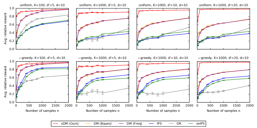
Figure 4: The relative reward of the learned policy on synthetic problems with varying $n$, $K$ and $d^{\prime}$ and varying logging policies.

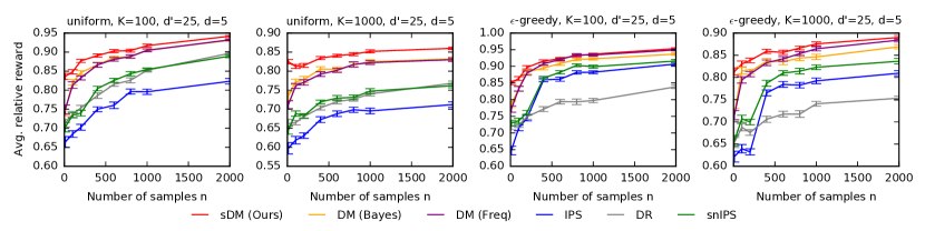
Figure 5: The relative reward of the learned policy on MovieLens problems with varying $n$ and $K$ and varying logging policies.

References

• Abbasi-Yadkori et al. (2011) Abbasi-Yadkori, Y., Pal, D., and Szepesvari, C. Improved algorithms for linear stochastic bandits. In Advances in Neural Information Processing Systems 24, pp.  2312–2320, 2011.
• Agrawal & Goyal (2013) Agrawal, S. and Goyal, N. Thompson sampling for contextual bandits with linear payoffs. In Proceedings of the 30th International Conference on Machine Learning, pp.  127–135, 2013.
• Aouali (2023) Aouali, I. Linear diffusion models meet contextual bandits with large action spaces. In NeurIPS 2023 Foundation Models for Decision Making Workshop, 2023.
• Aouali et al. (2022) Aouali, I., Hammou, A. A. S., Ivanov, S., Sakhi, O., Rohde, D., and Vasile, F. Probabilistic rank and reward: A scalable model for slate recommendation, 2022.
• Aouali et al. (2023a) Aouali, I., Brunel, V.-E., Rohde, D., and Korba, A. Exponential smoothing for off-policy learning. arXiv preprint arXiv:2305.15877, 2023a.
• Aouali et al. (2023b) Aouali, I., Kveton, B., and Katariya, S. Mixed-effect thompson sampling. In International Conference on Artificial Intelligence and Statistics, pp.  2087–2115. PMLR, 2023b.
• Auer et al. (2002) Auer, P., Cesa-Bianchi, N., and Fischer, P. Finite-time analysis of the multiarmed bandit problem. Machine Learning, 47:235–256, 2002.
• Bang & Robins (2005) Bang, H. and Robins, J. M. Doubly robust estimation in missing data and causal inference models. Biometrics, 61(4):962–973, 2005.
• Bottou et al. (2013) Bottou, L., Peters, J., Quiñonero-Candela, J., Charles, D. X., Chickering, D. M., Portugaly, E., Ray, D., Simard, P., and Snelson, E. Counterfactual reasoning and learning systems: The example of computational advertising. Journal of Machine Learning Research, 14(11), 2013.
• Chu et al. (2011) Chu, W., Li, L., Reyzin, L., and Schapire, R. Contextual bandits with linear payoff functions. In Proceedings of the 14th International Conference on Artificial Intelligence and Statistics, pp.  208–214, 2011.
• De Asis et al. (2023) De Asis, K., Graves, E., and Sutton, R. S. Value-aware importance weighting for off-policy reinforcement learning. arXiv preprint arXiv:2306.15625, 2023.
• Dudík et al. (2011) Dudík, M., Langford, J., and Li, L. Doubly robust policy evaluation and learning. International Conference on Machine Learning, 2011.
• Dudík et al. (2012) Dudík, M., Erhan, D., Langford, J., and Li, L. Sample-efficient nonstationary policy evaluation for contextual bandits. In Proceedings of the Twenty-Eighth Conference on Uncertainty in Artificial Intelligence, UAI’12, pp.  247–254, Arlington, Virginia, USA, 2012. AUAI Press.
• Dudik et al. (2014) Dudik, M., Erhan, D., Langford, J., and Li, L. Doubly robust policy evaluation and optimization. Statistical Science, 29(4):485–511, 2014.
• Farajtabar et al. (2018) Farajtabar, M., Chow, Y., and Ghavamzadeh, M. More robust doubly robust off-policy evaluation. In International Conference on Machine Learning, pp.  1447–1456. PMLR, 2018.
• Gilotte et al. (2018) Gilotte, A., Calauzènes, C., Nedelec, T., Abraham, A., and Dollé, S. Offline a/b testing for recommender systems. In Proceedings of the Eleventh ACM International Conference on Web Search and Data Mining, pp.  198–206, 2018.
• Hanna et al. (2019) Hanna, J., Niekum, S., and Stone, P. Importance sampling policy evaluation with an estimated behavior policy. In International Conference on Machine Learning, pp.  2605–2613. PMLR, 2019.
• Hong et al. (2023) Hong, J., Kveton, B., Zaheer, M., Katariya, S., and Ghavamzadeh, M. Multi-task off-policy learning from bandit feedback. In International Conference on Machine Learning, pp.  13157–13173. PMLR, 2023.
• Horvitz & Thompson (1952) Horvitz, D. G. and Thompson, D. J. A generalization of sampling without replacement from a finite universe. Journal of the American statistical Association, 47(260):663–685, 1952.
• Ionides (2008) Ionides, E. L. Truncated importance sampling. Journal of Computational and Graphical Statistics, 17(2):295–311, 2008.
• Jeunen & Goethals (2021) Jeunen, O. and Goethals, B. Pessimistic reward models for off-policy learning in recommendation. In Fifteenth ACM Conference on Recommender Systems, pp.  63–74, 2021.
• Jin et al. (2021) Jin, Y., Yang, Z., and Wang, Z. Is pessimism provably efficient for offline rl? In International Conference on Machine Learning, pp.  5084–5096. PMLR, 2021.
• Koller & Friedman (2009) Koller, D. and Friedman, N. Probabilistic Graphical Models: Principles and Techniques. MIT Press, Cambridge, MA, 2009.
• Kuzborskij et al. (2021) Kuzborskij, I., Vernade, C., Gyorgy, A., and Szepesvári, C. Confident off-policy evaluation and selection through self-normalized importance weighting. In International Conference on Artificial Intelligence and Statistics, pp.  640–648. PMLR, 2021.
• Lam & Herlocker (2016) Lam, S. and Herlocker, J. MovieLens Dataset. http://grouplens.org/datasets/movielens/, 2016.
• Lattimore & Szepesvari (2019) Lattimore, T. and Szepesvari, C. Bandit Algorithms. Cambridge University Press, 2019.
• Laurent & Massart (2000) Laurent, B. and Massart, P. Adaptive estimation of a quadratic functional by model selection. Annals of Statistics, pp.  1302–1338, 2000.
• Lazaric & Ghavamzadeh (2010) Lazaric, A. and Ghavamzadeh, M. Bayesian multi-task reinforcement learning. In ICML-27th international conference on machine learning, pp.  599–606. Omnipress, 2010.
• Li et al. (2010) Li, L., Chu, W., Langford, J., and Schapire, R. A contextual-bandit approach to personalized news article recommendation. In Proceedings of the 19th International Conference on World Wide Web, 2010.
• London & Sandler (2019) London, B. and Sandler, T. Bayesian counterfactual risk minimization. In International Conference on Machine Learning, pp.  4125–4133. PMLR, 2019.
• Metelli et al. (2021) Metelli, A. M., Russo, A., and Restelli, M. Subgaussian and differentiable importance sampling for off-policy evaluation and learning. Advances in Neural Information Processing Systems, 34:8119–8132, 2021.
• Robins & Rotnitzky (1995) Robins, J. M. and Rotnitzky, A. Semiparametric efficiency in multivariate regression models with missing data. Journal of the American Statistical Association, 90(429):122–129, 1995.
• Russo & Van Roy (2014) Russo, D. and Van Roy, B. Learning to optimize via posterior sampling. Mathematics of Operations Research, 39(4):1221–1243, 2014.
• Russo et al. (2018) Russo, D., Van Roy, B., Kazerouni, A., Osband, I., and Wen, Z. A tutorial on Thompson sampling. Foundations and Trends in Machine Learning, 11(1):1–96, 2018.
• Sachdeva et al. (2020) Sachdeva, N., Su, Y., and Joachims, T. Off-policy bandits with deficient support. In Proceedings of the 26th ACM SIGKDD International Conference on Knowledge Discovery & Data Mining, pp.  965–975, 2020.
• Saito & Joachims (2022) Saito, Y. and Joachims, T. Off-policy evaluation for large action spaces via embeddings. arXiv preprint arXiv:2202.06317, 2022.
• Sakhi et al. (2020) Sakhi, O., Bonner, S., Rohde, D., and Vasile, F. Blob: A probabilistic model for recommendation that combines organic and bandit signals. In Proceedings of the 26th ACM SIGKDD International Conference on Knowledge Discovery & Data Mining, pp.  783–793, 2020.
• Sakhi et al. (2022) Sakhi, O., Chopin, N., and Alquier, P. Pac-bayesian offline contextual bandits with guarantees. arXiv preprint arXiv:2210.13132, 2022.
• Schillings et al. (2020) Schillings, C., Sprungk, B., and Wacker, P. On the convergence of the laplace approximation and noise-level-robustness of laplace-based monte carlo methods for bayesian inverse problems. Numerische Mathematik, 145:915–971, 2020.
• Schlegel et al. (2019) Schlegel, M., Chung, W., Graves, D., Qian, J., and White, M. Importance resampling for off-policy prediction. Advances in Neural Information Processing Systems, 32, 2019.
• Spiegelhalter & Lauritzen (1990) Spiegelhalter, D. J. and Lauritzen, S. L. Sequential updating of conditional probabilities on directed graphical structures. Networks, 20(5):579–605, 1990.
• Su et al. (2019) Su, Y., Wang, L., Santacatterina, M., and Joachims, T. Cab: Continuous adaptive blending for policy evaluation and learning. In International Conference on Machine Learning, pp.  6005–6014. PMLR, 2019.
• Su et al. (2020) Su, Y., Dimakopoulou, M., Krishnamurthy, A., and Dudík, M. Doubly robust off-policy evaluation with shrinkage. In International Conference on Machine Learning, pp.  9167–9176. PMLR, 2020.
• Swaminathan & Joachims (2015a) Swaminathan, A. and Joachims, T. Batch learning from logged bandit feedback through counterfactual risk minimization. The Journal of Machine Learning Research, 16(1):1731–1755, 2015a.
• Swaminathan & Joachims (2015b) Swaminathan, A. and Joachims, T. The self-normalized estimator for counterfactual learning. advances in neural information processing systems, 28, 2015b.
• Swaminathan et al. (2017) Swaminathan, A., Krishnamurthy, A., Agarwal, A., Dudik, M., Langford, J., Jose, D., and Zitouni, I. Off-policy evaluation for slate recommendation. Advances in Neural Information Processing Systems, 30, 2017.
• Thompson (1933) Thompson, W. R. On the likelihood that one unknown probability exceeds another in view of the evidence of two samples. Biometrika, 25(3-4):285–294, 1933.
• Wang et al. (2023) Wang, L., Krishnamurthy, A., and Slivkins, A. Oracle-efficient pessimism: Offline policy optimization in contextual bandits. arXiv preprint arXiv:2306.07923, 2023.
• Wang et al. (2017) Wang, Y.-X., Agarwal, A., and Dudık, M. Optimal and adaptive off-policy evaluation in contextual bandits. In International Conference on Machine Learning, pp.  3589–3597. PMLR, 2017.
• Weiss (2005) Weiss, N. A Course in Probability. Addison-Wesley, 2005.
• Zhu et al. (2022) Zhu, Y., Foster, D. J., Langford, J., and Mineiro, P. Contextual bandits with large action spaces: Made practical. In International Conference on Machine Learning, pp.  27428–27453. PMLR, 2022.
• Zong et al. (2016) Zong, S., Ni, H., Sung, K., Ke, N. R., Wen, Z., and Kveton, B. Cascading bandits for large-scale recommendation problems. arXiv preprint arXiv:1603.05359, 2016.