On electroweak corrections to neutral current Drell–Yan with the POWHEG BOX

Abstract

Motivated by the requirement of a refined and flexible treatment of electroweak corrections to the neutral current Drell-Yan process, we report on recent developments on various input parameter/renormalization schemes for the calculation of fully differential cross sections, including both on-shell and $\overline{\rm MS}$ schemes. The latter are particularly interesting for direct determinations of running couplings at the highest LHC energies. The calculations feature next-to-leading order precision with additional higher order contributions from universal corrections such as $\Delta\alpha$ and $\Delta\rho$. All the discussed input parameter/renormalization scheme options are implemented in the package of POWHEG-BOX-V2 dedicated do the neutral current Drell-Yan simulation, i.e. Z_ew-BMNNPV, which is used to obtain the presented numerical results. In particular, a comprehensive analysis on physical observables calculated with different input parameter/renormalization     schemes is presented, addressing the $Z$ peak invariant mass region as well as the high energy window. We take the opportunity of reporting also on additional improvements and options introduced in the package Z_ew-BMNNPV after svn revision 3376, such as different options for the treatment of the hadronic contribution to the running of the electromagnetic coupling and for the handling of the unstable $Z$ resonance.

1 Introduction

The neutral current Drell-Yan (NC DY) process plays a particular role in the precision physics programme of the LHC. In fact, considering its large cross section and clean experimental signature, together with the high precision measurement of the $Z$-boson mass at LEP, this process is a standard candle that can be used for different general purposes such as detector calibration, Parton Distribution Functions (PDFs) constraining and tuning of non-perturbative parameters in the general purpose Monte Carlo event generators. Moreover, in the high tail of the transverse momentum and invariant mass distributions of the produced leptons, the NC DY is one of the main irreducible backgrounds to the searches for New Physics at the LHC. Recently an impressive precision at the sub-percent level has been reached by the experimental analysis in large regions of the dilepton phase space.

In addition to the above general aspects, it has to be stressed that the NC DY process also allows to perform precision tests of the Standard Model electroweak (SM EW) parameters through the direct determination of the $W$-boson mass CDF:2013dpa ; ATLAS:2017rzl ; CDF:2022hxs ; ATLAS:2023fsi and the weak mixing angle in hadronic collisions CMS:2011utm ; ATLAS:2015ihy ; LHCb:2015jyu ; CDF:2018cnj ; CMS:2018ktx . While in the former case the NC DY observables enter only indirectly, the latter can be determined directly, without reference to the charged current DY process. Another interesting possibility is the direct determination of the running of the coupling $\sin^{2}\theta$, defined in the $\overline{\rm MS}$ scheme, at the highest available LHC energies, in order to check its consistency with low energy and $Z$-peak measurements within the SM framework Amoroso:2023uux .

For all the above reasons, many efforts have been dedicated to the calculation of DY observables with the most advanced calculation techniques. On the perturbative side, the differential cross section, fully exclusive in the leptonic kinematical variables, is known with next-to-next-to-leading order (NNLO) accuracy in QCD Hamberg:1990np ; Gavin:2012sy ; Gavin:2010az ; Catani:2009sm ; Melnikov:2006kv ; Melnikov:2006di ; Anastasiou:2003ds and next-to-leading order (NLO) accuracy in the electroweak sector (EW) of the Standard Model (SM) Baur:1997wa ; Zykunov:2001mn ; Baur:2001ze ; Dittmaier:2001ay ; Baur:2004ig ; Arbuzov:2005dd ; CarloniCalame:2006zq ; Zykunov:2005tc ; CarloniCalame:2007cd ; Arbuzov:2007db ; Brensing:2007qm ; Dittmaier:2009cr ; Boughezal:2013cwa . Threshold effects at next-to-next-to-next-to-leading order (N³LO) in QCD have been studied in Refs. Ahmed:2014cla ; Catani:2014uta . First calculations of inclusive N³LO QCD corrections have been calculated for charged current DY in Ref. Duhr:2020sdp and for the production of a lepton pair mediated by photon exchange in Ref. Duhr:2020seh . The N³LO QCD corrections to the inclusive NC DY process have been calculated in Refs. Duhr:2021vwj ; Baglio:2022wzu while N³LO QCD corrections to single-differential distributions appeared in Refs. Chen:2021vtu ; Chen:2022lwc for neutral and charged current DY, respectively, and the N³LO QCD corrections to fiducial cross sections have been calculated in Refs. Chen:2022cgv ; Neumann:2022lft . The resummation of large logarithms due to soft gluon emission at small transverse momenta has been investigated in Refs. Neumann:2022lft ; Guzzi:2013aja ; Kulesza:2001jc ; Catani:2015vma ; Balazs:1997xd ; Landry:2002ix ; Cieri:2015rqa ; Bozzi:2010xn ; Mantry:2010mk ; Becher:2011xn ; Bizon:2018foh ; Bizon:2019zgf ; Re:2021con ; Ju:2021lah ; Camarda:2021ict ; Camarda:2023dqn ; Isaacson:2023iui , while the combined effects of QED and QCD transverse momentum resummation for $W$ and $Z$ production has been addressed in Ref. Cieri:2018sfk ; Autieri:2023xme . Relevant effects due to multiphoton emission have been studied in Refs. Placzek:2003zg ; CarloniCalame:2003ux ; CarloniCalame:2007cd ; Brensing:2007qm ; Dittmaier:2009cr . The mixed NNLO contributions of ${\cal O}(\alpha_{s}\alpha)$ have been evaluated in pole approximation for neutral and charged current DY Dittmaier:2014qza ; Dittmaier:2015rxo ; Dittmaier:2024row while the complete corrections of ${\cal O}(N_{f}\alpha_{s}\alpha)$ have been presented in Ref. Dittmaier:2020vra . Several results on ${\cal O}(\alpha_{s}\alpha)$ corrections to DY are available in narrow width approximation: QCD$\times$QED deFlorian:2018wcj , QCD$\times$EW Bonciani:2019nuy ; Bonciani:2020tvf ; Bonciani:2021iis corrections to inclusive $Z$ production and QCD$\times$EW corrections to fully exclusive $Z$ Delto:2019ewv ; Buccioni:2020cfi ; Cieri:2020ikq and $W$ production Behring:2020cqi . More recently important progress has been achieved on the necessary ingredients for the calculation of ${\cal O}(\alpha_{s}\alpha)$ corrections to the off-shell DY processes Bonciani:2016ypc ; Heller:2019gkq ; Hasan:2020vwn ; Heller:2020owb . The complete mixed ${\cal O}(\alpha_{s}\alpha)$ NNLO corrections to the NC DY process has been reported for the first time in Refs. Bonciani:2021zzf ; Armadillo:2022bgm ; Armadillo:2022ugh ; Buccioni:2022kgy , while, for the charged current DY process, they have been calculated in approximate form, i.e. neglecting the exact NNLO virtual contribution, in Ref. Buonocore:2021rxx .

Several fixed-order simulation tools have been developed, dedicated to NNLO QCD corrections like DYNNLO Catani:2009sm , DYTURBO Camarda:2019zyx , FEWZ Melnikov:2006kv ; Gavin:2010az , MATRIX Grazzini:2017mhc and MCFM Boughezal:2016wmq and to NLO EW corrections, like HORACE CarloniCalame:2006zq ; CarloniCalame:2007cd and ZGRAD/ ZGRAD2 Baur:1997wa ; Baur:2001ze , while the SANC framework Arbuzov:2007db ; Andonov:2008ga ; Bardin:2012jk ; Bondarenko:2013nu ; Arbuzov:2015yja ; Arbuzov:2016wfy ; Arbuzov:2022sep and the RADY code Dittmaier:2009cr allow to evaluate both QCD and EW NLO corrections. NNLO QCD corrections were combined with NLO EW contributions in FEWZ Li:2012wn . The state of the art of electroweak corrections in the form of form factors (featuring (N)NLO accuracy (at)/off the $Z$-resonance) are available in the libraries DIZET Arbuzov:2023afc and GRIFFIN Chen:2022dow .

A fundamental role in simulations for collider phenomenology is played by Monte Carlo event generators capable to consistently match fixed order calculations to parton showers (PS) simulating multiple soft/collinear radiations. The MC@NLO Frixione:2002ik and POWHEG Nason:2004rx ; Frixione:2007vw algorithms have been developed for the matching of NLO QCD computations to QCD PS and implemented in the public softwares MadGraph5_aMC@NLO Alwall:2014hca and POWHEG-BOX Alioli:2010xd ; Jezo:2015aia . Alternative formulations of the above algorithms are used in event generators like Sherpa Hoeche:2011fd ; Sherpa:2019gpd and HERWIG Bellm:2015jjp ; Platzer:2011bc . More recently, algorithms like NNLOPS Hamilton:2013fea (based on reweighting of the MiNLO^′ Hamilton:2012rf merging strategy), UNNLOPS Hoche:2014uhw ; Hoche:2014dla , Geneva Alioli:2013hqa , and MiNNLO_PS Monni:2019whf ; Monni:2020nks have been proposed for the matching of NNLO QCD calculations to QCD PS. Though several studies appeared on the approximated inclusion of EW corrections in event generators including higher-order QCD corrections (see, for instance Refs. Gutschow:2018tuk ; Brauer:2020kfv ; Lindert:2022qdd ), event generators including both NLO QCD and NLO EW corrections consistently matched to both QCD and QED parton showers are only available for a limited number of processes, namely: charged and neutral current Drell-Yan Barze:2012tt ; Bernaciak:2012hj ; Barze:2013fru ; Muck:2016pko ; Chiesa:2019nqb , $HV+0/1$ jet Chiesa:2019nqb , diboson production Chiesa:2020ttl , and electroweak $H+2$jets production Jager:2022acp . QED correction exclusive exponentiation for DY processes within YFS framework is realized within the event generator KKMC-hh Jadach:2016zsp ; Jadach:2017sqv ; Yost:2019bmz ; Yost:2020jin ; Yost:2022kxg .

The first implementation of QCD and EW NLO corrections and their interplay in a unique simulation framework has been given in Ref. Barze:2012tt for charged current DY  and in Ref. Barze:2013fru for NC DY. An important improvement in the matching of QED radiation in the presence of a resonance, following the ideas presented in Ref. Jezo:2015aia , has been discussed in Ref. CarloniCalame:2016ouw for the charged current DY process (W_ew-BMNNP svn revision 3375) and extended to the NC one (Z_ew-BMNNPV svn revision 3376) . After the above mentioned release, additional improvements and options have been introduced, in particular for the NC DY package Z_ew-BMNNPV, motivated by the need of a refined and flexible treatment of EW corrections that allows a consistent internal estimate of the uncertainties affecting the theoretical predictions. They can be schematically enumerated as follows:

• input parameter/renormalization schemes

• introduction of known higher order corrections

• treatment of the hadronic contribution to the running of the electromagnetic coupling $\Delta\alpha_{\rm had}$

• scheme for the treatment of the unstable resonance

In the following we give a detailed description of the various input parameter schemes and the related higher order corrections. A key ingredient of the latter is given by the running of the electromagnetic coupling $\alpha$ between different scales. In particular, when low scales are involved in the running, the hadronic contribution is intrinsically non-perturbative and different parametrizations have been developed in the literature relying on low-energy experimental data, which we properly include in our formulation of the electroweak corrections.

The formulae relevant for the various input parameters/ renormalization schemes are presented in a complete and self-contained form, so that they can be implemented in any simulation tool.

Though the Z_ew-BMNNPV package allows to simulate NC DY production at NLO QCD$+$NLO EW accuracy with consistent matching to the QED and QCD parton showers provided by PYTHIA8 Sjostrand:2006za ; Sjostrand:2014zea and/or Photos Golonka:2005pn ; Barberio:1990ms ; Barberio:1993qi , in the present paper we are mainly interested in various aspects of the fixed-order calculation (NLO EW plus universal higher orders). For this reason we show numerical results obtained at fixed-order and including only the weak corrections, since the QED contributions are not affected by the choice of the input parameter scheme and are a gauge-invariant subset of the EW corrections for the NC DY process.

The layout of the paper is the following: Section 2 provides an introduction to the input parameter schemes available in the code, while general considerations on higher order universal corrections, common to all the schemes, are presented in Section 3. A detailed account of various input/renormalization schemes at NLO accuracy and the related higher order corrections is given in Section 4, while a numerical analysis of the features of the schemes, with reference to cross section and forward-backward asymmetry, as functions of the dilepton invariant mass, is presented in Section 5, together with a discussion on the main parametric uncertainties in Section 6. The treatment of the hadronic contribution to the running of $\alpha$ is discussed in Section 7, while Section 8 is devoted to the description of the improvement of the code with respect to the treatment of the unstable $Z$ resonance. In Section 9 we analyse the effect of the various input/renormalization schemes in the high energy regimes, which will be accessible to the HL-LHC phase and future FCC-hh. A brief summary is given in Section 10. The list of the default parameter values  is contained in A, while the list of the flags activating the available options is given in B.

2 Input parameter schemes: general considerations

The input parameter schemes available in the Z_ew-BMNNPV package of POWHEG-BOX-V2 can be divided in three categories: the ones including both the $W$ and the $Z$ boson masses among the independent parameters, the $(\alpha_{0}$, $G_{\mu}$, $M_{Z})$ scheme, where we use the notation $\alpha_{0}$ for the QED coupling constant at $Q^{2}=0$, and the schemes with $M_{Z}$ and the sine of the weak mixing angle as free parameters. The latter class includes the schemes that use $\sin\theta_{eff}^{\ell}$ as input parameter, where $\theta_{eff}^{\ell}$ is the effective weak mixing angle, and an hybrid $\overline{\rm MS}$ scheme where the independent quantities are $\alpha_{\overline{MS}}(\mu^{2})$, $\sin^{2}\theta_{\overline{MS}}(\mu^{2})$ and $M_{Z}$, with the couplings renormalized in the $\overline{\rm MS}$ scheme and $M_{Z}$ with the usual on-shell prescription.

The first class of input parameter schemes, namely $(\alpha_{i}$, $M_{W}$, $M_{Z})$ with $\alpha_{i}=\alpha_{0}$, $\alpha(M_{Z}^{2})$, $G_{\mu}$, is widely used for the calculation of the EW corrections for processes of interest at the LHC. On the one hand, the fact that the $W$ boson mass is a free parameter is a useful feature, in particular, in view of the experimental determination of $M_{W}$ from charged current Drell-Yan production using template fit methods; on the other hand, the predictions obtained in these schemes can suffer from relatively large parametric uncertainties related to the current experimental precision on $M_{W}$. This drawback is overcome, for instance, in the $(\alpha_{0}$, $G_{\mu}$, $M_{Z})$ scheme used for the calculation of the EW corrections in the context of LEP physics, where all the input parameters are experimentally known with high precision. The third class of input parameter schemes uses the sine of the weak mixing angle as a free parameter. In the Z_ew-BMNNPV package the $(\alpha_{i}$, $\sin\theta_{eff}^{\ell}$, $M_{Z})$ schemes, with $\alpha_{i}=\alpha_{0}$, $\alpha(M_{Z}^{2})$, $G_{\mu}$, and the $(\alpha_{\overline{MS}}(\mu)$, $\sin^{2}\theta_{\overline{MS}}(\mu^{2})$, $M_{Z})$ one are implemented. The schemes where $\sin\theta_{eff}^{\ell}$ $(\sin^{2}\theta_{\overline{MS}}(\mu^{2}))$ is a free parameter are particularly useful in the context of the experimental determination of $\sin\theta_{eff}^{\ell}$ $(\sin^{2}\theta_{{\overline{MS}}}(\mu^{2}))$ from NC DY production at the LHC using template fits Chiesa:2019nqb ; Amoroso:2023uux .

The predictions for NC DY production obtained in the schemes that use $\alpha(M_{Z}^{2})$ or $G_{\mu}$ as inputs show a better convergence of the perturbative series compared to the corresponding results from the schemes with $\alpha_{0}$ as free parameter . This is a consequence of the fact that, when using $\alpha(M_{Z}^{2})$ or $G_{\mu}$ as independent variables, large parts of the radiative corrections related to the running of $\alpha(Q^{2})$ from $Q^{2}=0$ to the electroweak scale are reabsorbed in the LO predictions. On the contrary, the EW corrections in the schemes with $\alpha_{0}$ as input tend to be larger, because the running of $\alpha(Q^{2})$ involves logarithmic corrections of the form $\log(m^{2}/Q^{2})$, where $m$ stands for the light-fermion masses (we refer to Sect. 7 for the treatment of the light-quark contributions to the running of $\alpha(Q^{2})$) and $Q^{2}$ stands for the typical large mass scale of the process.

From a technical point of view, the calculation of the one-loop electroweak corrections in the above-mentioned input parameter schemes differs in the renormalization prescriptions used for the computation, while the bare part of the Drell-Yan amplitudes remains formally the same and it is just evaluated with different numerical values of the input parameters. For each choice of input scheme, the renormalization is performed as follows: first the electroweak parameters are expressed as a function of the three selected independent quantities, then the counterterms corresponding to these parameters are fixed by imposing some renormalization condition, and finally the counterterms for the derived electroweak parameters are written in terms of the ones corresponding to the input parameters.

The fact that the counterterm part of the Drell-Yan amplitude differs in the considered input parameter schemes implies that also the expression of the universal fermionic corrections changes, as these corrections at NLO can be related to the counterterm amplitude. In fact, they can be computed at $\mathcal{O}(\alpha^{2})$ taking the square of the fermionic universal contributions at NLO (after subtracting the $\mathcal{O}(\alpha)$ terms already included in the NLO calculation). We refer to Sect. 3 for details.

The input parameter schemes described in the following sections are formally equivalent for a given order in perturbation theory; however, the numerical results obtained differ because of the truncation of the perturbative expansion. Although there is some arbitrariness in the choice of the input parameter scheme to be used for the calculations, there can be phenomenological motivations to prefer one scheme to the others, depending on the observables under consideration and on the role played by the theory predictions with respect to the interpretation of the experimental measurements. For instance, in the context of cross section or distribution measurements, where the theory predictions are used as a benchmark for the experimental results but do not provide input for parameter determination, those input parameter schemes should be preferred that involve independent quantities known experimentally with high precision in order to minimize the corresponding parametric uncertainties. One should also try to minimize the parametric uncertainties from quantities that enter the calculation only at loop level (such as, for instance, the top quark mass in DY processes). Another aspect that should be taken into account when choosing an input parameter scheme is the convergence of the perturbative expansion in the predictions for the observables of interest, which is mainly related to the possibility of reabsorbing large parts of the radiative corrections in the definition of the coupling at LO.

A different situation is the direct determination of electroweak parameters using template fit methods, as done for example for the $W$ boson mass at Tevatron and LHC. In this case, the theory predictions enter the interpretation of the measurement (with the Monte Carlo templates) and the theory uncertainties become part of the total systematic error on the quantity under consideration: it is thus important to use an input parameter scheme where the quantity to be measured is a free parameter that can be varied independently not only at LO, but also at higher orders in perturbation theory.

3 Higher-order corrections

At moderate energies, the leading corrections to NC DY production are related to the logarithms of the light fermion masses and to terms proportional to the top quark mass squared. These contributions can be traced back to the running of $\alpha(Q^{2})$ (i.e. to $\Delta\alpha$) and to $\Delta\rho$ and are thus related to the counterterm amplitude for the process under consideration. Following Refs. Consoli:1989fg ; Denner:1991kt ; Diener:2005me ; Dittmaier:2009cr , these effects can be taken into account at $\mathcal{O}(\alpha^{2})$ by taking the square of the part of the counterterm amplitude proportional to $\Delta\alpha$ and $\Delta\rho$. They can thus be combined to the full NLO calculation after subtracting the part of linear terms in $\Delta\alpha$ and $\Delta\rho$ appearing in the square of the counterterm amplitude that are already present in the NLO computation.

The numerical results for the fermionic higher-order corrections presented in the following are obtained using the one-loop expression for $\Delta\alpha$ (even though the two-loop leptonic corrections are also available in the Z_ew-BMNNPV package and can be activated with the flag dalpha_lep_2loop), while for $\Delta\rho$ we include the leading Yukawa corrections up to $\mathcal{O}(\alpha_{S}^{2})$, $\mathcal{O}(\alpha_{S}x_{t}^{2})$, and $\mathcal{O}(x_{t}^{3})$, with $x_{t}=\sqrt{2}G_{\mu}M_{\rm top}^{2}/16\pi^{2}$. More precisely, the expression used for $\Delta\rho$ is

$$\Delta\rho^{HO} =3x_{t}(1+x_{t}\Delta\rho^{(2)})(1+\frac{\alpha_{S}}{\pi}\delta^{(2)}_{QCD}+\frac{\alpha_{S}^{2}}{\pi^{2}}\delta^{(3)}_{QCD})$$ (1)

$$+x_{t}^{3}\Delta\rho^{x_{t}^{3}}+\frac{\alpha_{S}}{\pi}x_{t}^{2}\Delta\rho^{x_{t}^{2}\alpha_{S}}-3x_{t}^{2}\Delta\rho^{(2)}\frac{\alpha_{S}}{\pi}\delta^{(2)}_{QCD},$$

where $\Delta\rho^{(2)}$ is the two-loop heavy-top corrections to the $\rho$ parameter Veltman:1977kh ; Fleischer:1993ub ; Fleischer:1994cb , $\delta^{(2)}_{QCD}$ and $\delta^{(3)}_{QCD}$ are the two and three-loop QCD corrections Djouadi:1987gn ; Djouadi:1987di ; Kniehl:1989yc ; Avdeev:1994db , while the three-loop contributions $\Delta\rho^{x_{t}^{3}}$ and $\Delta\rho^{x_{t}^{2}\alpha_{S}}$ are taken from Ref. Faisst:2003px . The last term in Eq. (1) is introduced in order to avoid the double counting of the $\mathcal{O}(x_{t}^{2}\alpha_{S}^{2})$ contribution already present in factorized approximation in the product of the QCD corrections and the Yukawa corrections at two loops. The four-loop QCD corrections to the $\rho$ parameter Chetyrkin:2006bj are not included. By inspection of the numerical impact of three-loop QCD corrections (cfr. Figs. 7 and 8), the phenomenological impact of four-loop QCD corrections to the $\rho$ parameter is expected to be negligible at the LHC. For the numerical studies presented in the following, the scale for the $\alpha_{S}$ factors entering the QCD corrections to $\Delta\rho$ is set to the invariant mass of the dilepton pair.

4 Input parameter schemes: detailed description

In the following subsections we present a detailed account of the available input parameter schemes at NLO weak accuracy and the related universal higher order corrections. In the last subsection we present a comparison of the radiative corrections obtained with the different parameter schemes for two relevant differential observables (cross section and forward-backward asymmetry as functions of the dilepton invariant mass $M(ll)$) of the NC DY process at the LHC with $\sqrt{s}=13$ TeV, considering $\mu^{+}\mu^{-}$ final states. In the following, for the sake of simplicity of notation, whenever the complex mass scheme is used for the treatment of the unstable gauge bosons, the symbol $M^{2}_{V}$, with $V=W,Z$, represents the quantity $\mu^{2}_{V}=M^{2}_{V}-i\Gamma_{V}M_{V}$.

4.1 The $(\alpha_{0}/\alpha(M_{Z}^{2})/G_{\mu}$, $M_{W}$, $M_{Z})$ schemes

In these schemes, the input parameters are the $W$ and $Z$ boson masses and $\alpha_{i}=\alpha_{0}$, $\alpha(M_{Z}^{2})$, $G_{\mu}$. The counterterms for the independent parameters are defined as

$$M_{Z,b}^{2} = M_{Z}^{2}+\delta M_{Z}^{2}$$ (2)

$$M_{W,b}^{2} = \mbox{$M_{W}^{2}$}+\delta\mbox{$M_{W}^{2}$}$$ (3)

$$e_{b} = e(1+\delta Z_{e})\,,$$ (4)

where the subscript $b$ denotes the bare parameter. The expression for $\delta Z_{e}$ is fixed by imposing that the NLO EW corrections to the $\gamma e^{+}e^{-}$ vertex vanish in the Thomson limit, while $\delta\mbox{$M_{W}^{2}$}$ and $\delta M_{Z}^{2}$ are obtained by requiring that the gauge-boson masses do not receive radiative corrections.

The analytic expression of the counterterms can be found in Ref. Denner:1991kt (and in Refs. Denner:1999gp ; Denner:2005fg ; Denner:2006ic if the complex-mass scheme is used). In the following, for the self energies and the counterterms we will use the notation of Ref. Denner:1991kt .

In the schemes with $M_{W}$ and $M_{Z}$ as independent parameters, the sine of the weak-mixing angle is a derived quantity defined as

$$s_{W}^{2}=1-\frac{M_{W}^{2}}{M_{Z}^{2}},$$ (5)

and the corresponding counterterm reads:

$$\frac{\delta s_{W}}{s_{W}}=-\frac{1}{2}\frac{c_{W}^{2}}{s_{W}^{2}}\Big{(}\frac{\delta M_{W}^{2}}{M_{W}^{2}}-\frac{\delta M_{Z}^{2}}{M_{Z}^{2}}\Big{)}.$$ (6)

When $\alpha(M_{Z}^{2})$ or $G_{\mu}$ are used as input parameters, the calculation of the $\mathcal{O}(\alpha)$ corrections is formally the same one as in the $(\alpha_{0}$, $M_{W}$, $M_{Z})$ scheme but with the replacements $\delta Z_{e}\to\delta Z_{e}-\Delta\alpha(M_{Z}^{2})/2$ and $\delta Z_{e}\to\delta Z_{e}-\Delta r/2$, respectively, that take into account the running of $\alpha(Q^{2})$ from $Q^{2}=0$ to the weak scale which is absorbed in the LO coupling ($\alpha(M_{Z}^{2})$ or $G_{\mu}$). It is worth noticing that these replacements remove the logarithmically enhanced fermionic corrections coming from $\Delta\alpha$. The factor $\Delta r$ represents the full one-loop electroweak corrections to the muon decay in the scheme $(\alpha_{0}$, $M_{W}$, $M_{Z})$ after the subtraction of the QED effects in the Fermi theory and reads:

$$\Delta r=\Delta\alpha-\frac{c_{W}^{2}}{s_{W}^{2}}\Delta\rho^{self}+\Delta r^{self}_{rem}=\Delta\alpha-\frac{c_{W}^{2}}{s_{W}^{2}}\Delta\rho+\Delta r_{rem},$$ (7)

with

$$\Delta\rho^{self} = \frac{\Sigma_{T}^{ZZ}(0)}{M_{Z}^{2}}-\frac{\Sigma_{T}^{WW}(0)}{M_{W}^{2}}=\frac{\alpha}{4\pi}\frac{3}{4s_{W}^{2}}\frac{M_{T}^{2}}{M_{W}^{2}}+\cdots$$ (8)

$$= \Delta\rho^{1-loop}|_{\alpha}+{\rm non-enhanced\;terms},$$

(clearly $\Delta\rho^{1-loop}|_{\alpha(G_{\mu})}=3x_{t}$) and

$$\Delta r_{rem}^{self}=\frac{{\rm Re}\Sigma^{AA}_{T}(s)}{s}-\frac{c_{W}^{2}}{s_{W}^{2}}\left(\frac{\delta M_{Z}^{2}}{M_{Z}^{2}}-\frac{\Sigma_{T}^{ZZ}(0)}{M_{Z}^{2}}\right)$$ (9)

$$+ \frac{c_{W}^{2}-s_{W}^{2}}{s_{W}^{2}}\left(\frac{\delta M_{W}^{2}}{M_{W}^{2}}-\frac{\Sigma_{T}^{WW}(0)}{M_{W}^{2}}\right)+2\frac{c_{W}}{s_{W}}\frac{\Sigma_{T}^{AZ}(0)}{M_{Z}^{2}}$$

$$+ \frac{\alpha}{4\pi s_{W}^{2}}\Big{(}6+\frac{7-4s_{W}^{2}}{2s_{W}^{2}}{\rm log}(c_{W}^{2})\Big{)}.$$

From the expression of the counterterms, one can notice that the leading fermionic corrections at NLO EW are related to

$$\delta Z_{e}\sim\frac{\Delta\alpha}{2},~{}~{}~{}\frac{\delta s_{W}}{s_{W}}\sim\frac{1}{2}\frac{c_{W}^{2}}{s_{W}^{2}}\Delta\rho,~{}~{}~{}\Delta r\sim\Delta\alpha-\frac{c_{W}^{2}}{s_{W}^{2}}\Delta\rho.$$ (10)

In the Z_ew-BMNNPV package, we implemented a slightly modified version of Eqs. (3.45)-(3.49) of Ref. Dittmaier:2009cr for the computation of the leading fermionic corrections to neutral-current Drell-Yan up to $\mathcal{O}(\alpha^{2})$. More precisely, those equations are modified in such a way to be valid also in the complex-mass scheme. As discussed in Sect. 3, in order to combine these higher-order fermionic corrections with the NLO EW results, it is mandatory to subtract those effects that are included in the full one-loop calculation to avoid double counting. In particular, this implies the replacement $\Delta\rho\to(\Delta\rho-\Delta\rho^{\rm 1-loop})$ in the linear terms of the fermionic corrections up to $\mathcal{O}(\alpha^{2})$: if we use, optionally by means of the flag a2a0-for-QED-only , for the overall weak-loop factors the same value of $\alpha_{i}$ used in the LO couplings, $\Delta\rho^{\rm 1-loop}$ is computed as a function of $\alpha_{0}$, $\alpha(M_{Z}^{2})$, or $G_{\mu}$ for the $(\alpha_{0}$, $M_{W}$, $M_{Z})$, $(\alpha(M_{Z}^{2})$, $M_{W}$, $M_{Z})$, and $(G_{\mu}$, $M_{W}$, $M_{Z})$ schemes, respectively. If instead we use $\alpha_{0}$ for the overall weak-loop factors, we subtract the quantity $\Delta\rho^{\rm 1-loop}|^{\alpha_{0}}$ computed in the $\alpha_{0}$ scheme, regardless of the value of $\alpha_{i}$ used as independent parameter.

4.2 The $(\alpha_{0}/\alpha(M_{Z}^{2})/G_{\mu}$, $\sin^{2}\theta_{eff}^{\ell}\,$, $M_{Z})$ schemes

In the $(\alpha_{i}$, $\sin^{2}\theta_{eff}^{\ell}\,$, $M_{Z})$ schemes (where $\alpha_{i}=\alpha_{0}$, $\alpha(M_{Z}^{2})$, $G_{\mu}$) the sine of the effective weak mixing angle is used as input parameter . This quantity is defined from the ratio of the vectorial and axial-vectorial couplings of the $Z$ boson to the leptons $g_{V}^{\ell}$ and $g_{A}^{\ell}$, or, equivalently, in terms of the chiral $Zll$ couplings $g_{L}^{\ell}$ and $g_{R}^{\ell}$, measured at the $Z$ resonance and reads

$$\sin^{2}\theta_{eff}^{\ell}\,~{}\equiv~{}\frac{I_{3}^{l}}{Q_{l}}\,{\rm Re}\left(\frac{-g_{R}^{\ell}(M_{Z}^{2})}{g_{L}^{\ell}(M_{Z}^{2})-g_{R}^{\ell}(M_{Z}^{2})}\right)\,,$$ (11)

where ${I_{3}^{l}}$ is the third component of the weak isospin for left-handed leptons. Since $\sin^{2}\theta_{eff}^{\ell}\,$ is used as an independent parameter, this scheme is particularly useful in the context of the direct extraction of $\sin^{2}\theta_{eff}^{\ell}\,$ from NC DY at the LHC using template fit methods at NLO EW accuracy.

The counterterms corresponding to the input parameters are defined as

$$M_{Z,b}^{2} = M_{Z}^{2}+\delta M_{Z}^{2}$$ (12)

$$\sin^{2}\theta_{b} = \sin^{2}\theta_{eff}^{\ell}\,+\delta\sin^{2}\theta_{eff}^{\ell}\,$$ (13)

$$e_{b} = e(1+\delta Z_{e})\,.$$ (14)

The expressions of $\delta Z_{e}$ and $\delta M_{Z}^{2}$ are determined as in Sect. 4.1, while the expression of $\delta\sin^{2}\theta_{eff}^{\ell}\,$ is fixed by requiring that the definition in Eq. (11) holds to all orders in perturbation theory. More precisely, we write Eq. (11) at one loop as

$$\sin^{2}\theta_{eff}^{\ell}\,~{}\equiv~{}\frac{I_{3}^{l}}{Q_{l}}\,{\rm Re}\left(\frac{-{\cal G}_{R}^{\ell}(M_{Z}^{2})}{{\cal G}_{L}^{\ell}(M_{Z}^{2})-{\cal G}_{R}^{\ell}(M_{Z}^{2})}\right)\,$$ (15)

$$= \frac{1}{2}{\rm Re}\frac{-g_{R}}{g_{L}-g_{R}}+\frac{1}{2}{\rm Re}\frac{g_{L}g_{R}}{(g_{L}-g_{R})^{2}}\Big{(}\frac{\delta g_{L}}{g_{L}}-\frac{\delta g_{R}}{g_{R}}\Big{)}.$$

where $\mathcal{G}_{L(R)}(M_{Z}^{2})=g_{L(R)}+\delta g_{L(R)}(M_{Z}^{2})$ represent the $Zl^{L}l^{L}$ and $Zl^{R}l^{R}$ form factors computed at one loop accuracy at the scale $M_{Z}^{2}$ and we impose the condition:

$${\rm Re}\left(\frac{-{\cal G}_{R}^{\ell}(M_{Z}^{2})}{{\cal G}_{L}^{\ell}(M_{Z}^{2})-{\cal G}_{R}^{\ell}(M_{Z}^{2})}\right)={\rm Re}\left(\frac{-g_{R}^{\ell}}{g_{L}^{\ell}-g_{R}^{\ell}}\right),$$ (16)

which implies

$${\rm Re}\left(\frac{\delta g_{L}^{\ell}}{g_{L}^{\ell}}-\frac{\delta g_{R}^{\ell}}{g_{R}^{\ell}}\right)\,~{}=~{}0.$$ (17)

The $\delta g_{L(R)}$ factors contain both bare vertices and counterterms and since they are functions of $\delta\sin^{2}\theta_{eff}^{\ell}\,$, Eq. (17) can be used to compute the counterterm corresponding to the effective weak mixing angle. By inserting the expressions for $\delta g_{L(R)}$ one gets

$$\frac{\delta\sin^{2}\theta_{eff}^{\ell}\,}{\sin^{2}\theta_{eff}^{\ell}\,}={\rm Re}\Big{\{}-\frac{1}{2}\frac{\cos\theta_{eff}^{\ell}}{\sin\theta_{eff}^{\ell}}\delta Z_{AZ}$$ (18)

$$+\left(1-\frac{Q_{\ell}}{I_{3}^{\ell}}\sin^{2}\theta_{eff}^{\ell}\,\right)\left[\delta Z^{\ell}_{L}+\delta V^{L}-\delta Z^{\ell}_{R}-\delta V^{R}\right]\Big{\}},$$

where $\delta Z^{\ell}_{L(R)}$ are the pure weak parts of the wave function renormalization counterterms for the leptons and $\delta V^{L(R)}$ are the one-loop weak corrections to the left/right $Zll$ vertices defined as

$$\delta V^{L} = \left(g^{\ell}_{L}\right)^{2}\frac{\alpha}{4\pi}{\cal V}_{a}\left(0,M_{Z}^{2},0,M_{Z},0,0\right)$$

$$+ \frac{1}{2s_{W}^{2}}\frac{g^{\nu}_{L}}{g^{\ell}_{L}}\frac{\alpha}{4\pi}{\cal V}_{a}\left(0,M_{Z}^{2},0,M_{W},0,0\right)$$

$$- \frac{c_{W}}{s_{W}}\frac{1}{2s_{W}^{2}}\frac{1}{g^{\ell}_{L}}\frac{\alpha}{4\pi}{\cal V}_{b}\left(0,M_{Z}^{2},0,0,M_{W},M_{W}\right)$$

$$\delta V^{R} = \left(g^{\ell}_{R}\right)^{2}\frac{\alpha}{4\pi}{\cal V}_{a}\left(0,M_{Z}^{2},0,M_{Z},0,0\right)$$ (19)

and the vertex functions ${\cal V}_{a}$ and ${\cal V}_{b}$ are given in Eqs. (C.1) and (C.2) of Ref. Denner:1991kt , respectively. No QED correction is included in Eq. (18), since the QED contributions to the $Zll$ vertex are the same for left or right-handed fermions and cancel in Eq. (17). When the complex mass scheme is used, the input value for $\sin^{2}\theta_{eff}^{\ell}\,$ remains real: this implies that $g_{R/L}^{\rm LO}$ remain real and the condition (16) still reduces to (17). As a consequence, the definition in Eq. (18) remains valid in the complex-mass scheme, provided that the CMS expressions for $\delta Z^{\ell}_{L(R)}$ and $\delta Z_{AZ}$ are used. Note that the vertex functions ${\cal V}_{a}$ and ${\cal V}_{b}$ are computed for a real scale $M_{Z}^{2}$, while the gauge boson masses appearing in the loop diagrams are promoted to complex. If one instead uses a complex-valued $s_{W}^{2}$ (see the discussion on fermionic higher-order effects in Sect. 4.3), the condition in (17) can still be used but without taking the real part.

As already discussed in Sect. 4.1, the counterterms in the $(\alpha(M_{Z}^{2})$, $\sin^{2}\theta_{eff}^{\ell}\,$, $M_{Z})$ and $(G_{\mu}$, $\sin^{2}\theta_{eff}^{\ell}\,$, $M_{Z})$ schemes can be obtained from the ones in the $(\alpha_{0}$, $\sin^{2}\theta_{eff}^{\ell}\,$, $M_{Z})$ scheme performing the replacements $\delta Z_{e}\to\delta Z_{e}-\Delta\alpha(M_{Z}^{2})/2$ and $\delta Z_{e}\to\delta Z_{e}-\Delta\tilde{r}/2$, respectively, where $\Delta\tilde{r}$ represents the one-loop electroweak corrections to the muon decay (after subtracting the QED effects in the Fermi theory) in the scheme $(\alpha_{0}$, $\sin^{2}\theta_{eff}^{\ell}\,$, $M_{Z})$ and reads

$$\Delta\tilde{r}=2\delta Z_{e}-\Big{(}1-\frac{s_{W}^{2}}{c_{W}^{2}}\Big{)}\frac{\delta\sin^{2}\theta_{eff}^{\ell}\,}{s^{2}_{W}}-\frac{\delta M_{Z}^{2}}{M_{Z}^{2}}+\frac{\Sigma^{WW}_{T}(0)}{M_{W}^{2}}$$ (20)

$$+ \frac{2}{c_{W}s_{W}}\frac{\Sigma^{AZ}_{T}(0)}{M_{Z}^{2}}+\frac{\alpha}{4\pi s_{W}^{2}}\Big{(}6+\frac{7-4s_{W}^{2}}{2s_{W}^{2}}\log{c_{W}^{2}}\Big{)}$$

that can be written also as

$$\Delta\tilde{r}=\Delta\alpha-\Delta\rho^{self}+\Delta\tilde{r}^{self}_{rem}=\Delta\alpha-\Delta\rho+\Delta\tilde{r}_{rem},$$ (21)

with

$$\Delta\tilde{r}^{self}_{rem} = \frac{{\rm Re}\Sigma^{AA}_{T}(s)}{s}-\left(\frac{\delta M_{Z}^{2}}{M_{Z}^{2}}-\frac{\Sigma_{T}^{ZZ}(0)}{M_{Z}^{2}}\right)$$ (22)

$$+ \frac{s_{W}^{2}-c_{W}^{2}}{c_{W}^{2}}\frac{\delta\sin^{2}\theta_{eff}^{\ell}\,}{s_{W}^{2}}+2\frac{c_{W}}{s_{W}}\frac{\Sigma_{T}^{AZ}(0)}{M_{Z}^{2}}$$

$$+ \frac{\alpha}{4\pi s_{W}^{2}}\Big{(}6+\frac{7-4s_{W}^{2}}{2s_{W}^{2}}{\rm log}(c_{W}^{2})\Big{)},$$

where we used the short-hand notation $s_{W}=\sin\theta_{eff}^{\ell}$ and $c_{W}=\cos\theta_{eff}^{\ell}$.

From Eqs. (18)-(21) it is clear that the leading fermionic corrections in the schemes with $\sin^{2}\theta_{eff}^{\ell}\,$ as input parameter are only related to $\delta Z_{e}\sim\frac{\Delta\alpha}{2}$ and $\Delta\tilde{r}\sim\Delta\alpha-\Delta\rho$, while the counterterm of $\sin^{2}\theta_{eff}^{\ell}\,$ does not contain terms proportional to the logarithms of the light-fermion masses or to the square of the top quark mass. As a result, the fermionic higher-order corrections in these schemes (after the subtraction of the effects already included in the $\mathcal{O}(\alpha)$ calculation) are just overall factors that multiply the LO matrix element squared and read:

$$|M_{\rm LO}|^{2}\Big{(}\frac{1}{(1-\Delta\alpha(M_{Z}))^{2}}-1-2\Delta\alpha(M_{Z})\Big{)},$$ (23)

and

$$|M_{\rm LO}|^{2}\Big{(}\frac{1}{(1-\Delta\rho)^{2}}-1-2\Delta\rho^{(1)}\Big{)},$$ (24)

for the schemes with $\alpha_{0}$ and $G_{\mu}$ as input parameters, respectively, while these corrections are zero when $\alpha(M_{Z}^{2})$ is used as independent parameter. In equation (23), a resummation of the logarithms of the light-fermion masses was performed, while the overall factor in (24) comes from the relation between $\alpha$ and $G_{\mu}$ at NLO plus higher orders (NLO+HO), namely $\alpha=G_{\mu}s_{W}^{2}c_{W}^{2}M_{Z}^{2}\sqrt{2}(1+\Delta\tilde{r}-\Delta\alpha)/\pi$.

4.3 The $(\alpha_{0}$, $G_{\mu}$, $M_{Z})$ scheme

In the $(\alpha_{0}$, $G_{\mu}$, $M_{Z})$ scheme, the input parameters are $\alpha_{0}$, $G_{\mu}$, and the mass of the $Z$ boson. The main advantage of using this scheme is that all the independent parameters are experimentally known with high precision and the corresponding parametric uncertainties are small (in particular, compared to the schemes in Sect. 4.1, it is independent of the uncertainties related to the experimental knowledge of $M_{W}$).

In the scheme under consideration, the sine of the weak mixing angle and the $W$ boson mass are derived quantities. At the lowest order in perturbation theory they can be computed using the relations

$$(1-s_{W}^{2})s_{W}^{2}=\frac{\pi\alpha}{\sqrt{2}G_{\mu}M_{Z}^{2}},$$ (25)

$$c_{W}^{2}=1-s_{W}^{2},\qquad c_{W}^{2}=\frac{M_{W}^{2}}{M_{Z}^{2}},$$

$$s_{W}^{2}=\frac{1}{2}-\sqrt{\frac{1}{4}-\frac{\pi\alpha}{\sqrt{2}G_{\mu}M_{Z}^{2}}},\quad M_{W}^{2}=\frac{\pi\alpha}{\sqrt{2}G_{\mu}s_{W}^{2}}.$$ (26)

In terms of Eqs. (26), it is possible to write the LO amplitude for NC DY as the sum of the photon exchange amplitude proportional to $\alpha$ and the $Z$ exchange amplitude proportional to $G_{\mu}M_{Z}^{2}$, namely:

$$M^{\sigma,\tau}=A^{\sigma,\tau}\Big{[}-\frac{4\pi\alpha}{s}Q_{q}Q_{l}-\frac{4\sqrt{2}G_{\mu}M_{Z}^{2}}{s}G_{q}^{\sigma}G_{l}^{\tau}\chi_{Z}(s)\Big{]},$$ (27)

where $A^{\sigma,\tau}$ is the part of the amplitude containing the $\gamma$ matrices and the external fermions spinors ($\sigma,\tau=L,R$) and

$$G_{q(l)}^{\sigma}=I_{3}^{\sigma\,q(l)}-s_{W}^{2}Q_{q(l)},~{}~{}\chi_{Z}(s)=\frac{s}{s-M_{Z}^{2}+i\Gamma_{Z}M_{Z}},$$ (28)

$Q_{q(l)}$ and $I_{3}^{\sigma\,q(l)}$ being the quark (lepton) charges and third components of the weak isospin. In the complex-mass scheme, the definition of $\chi_{Z}$ is $s/(s-M_{Z}^{2})$. Clearly the $Z$-boson exchange diagram contains a residual dependence on $\alpha$ from $s_{W}$ in Eq. (28). Two different realizations of the $(\alpha_{0}$, $G_{\mu}$, $M_{Z})$ scheme are available in the Z_ew-BMNNPV package: users can select a specific one through the azinscheme4 flag in the powehg.input file. If the flag is absent or negative, in Eqs. (26) $\alpha=\alpha_{0}$ in such a way that the $\gamma f\bar{f}$ interaction is evaluated at low scale while the $Zf\bar{f}$ couplings are computed at the weak scale. If azinscheme4 is positive, $\alpha=\alpha_{0}/(1-\Delta\alpha(M_{Z}))$: this way also the photon part of the amplitude is evaluated at the weak scale. Note that we compute $\Delta\alpha(M_{Z})$ form $\alpha_{0}$ rather that taking $\alpha(M_{Z})$ as an independent parameter. For dilepton invariant masses in the resonance region or larger, the latter running mode allows to reabsorb in the couplings the mass logarithms originating from the running of $\alpha$ from $q^{2}=0$ to the weak scale. If not otherwise stated, the numerical results presented for the $(\alpha_{0}$, $G_{\mu}$, $M_{Z})$ scheme are obtained with azinscheme4$=1$.

The counterterms for the independent quantities are defined as:

$$M_{Z,b}^{2} = M_{Z}^{2}+\delta M_{Z}^{2}$$ (29)

$$G_{\mu,b} = G_{\mu}+\delta G_{\mu}$$ (30)

$$e_{b} = e(1+\delta Z_{e}).$$ (31)

The expression of the $\delta Z_{e}$ and $\delta M_{Z}^{2}$ counterterms is fixed as in Sect. 4.1 (if azinscheme4$=1$, there is the additional shift $\delta Z_{e}\to\delta Z_{e}-\Delta\alpha(M_{Z})/2$), while $\delta G_{\mu}$ is determined by requiring that the muon decay computed in the $(\alpha_{0}$, $G_{\mu}$, $M_{Z})$ scheme does not receive any correction at NLO (after the subtraction of the QED effects in the Fermi theory), namely:

$$\frac{\delta G_{\mu}}{G_{\mu}} = -\frac{2}{s_{W}c_{W}}\frac{\Sigma^{AZ}_{T}(0)}{M_{Z}^{2}}-\frac{\Sigma^{WW}_{T}(0)}{M_{W}^{2}}$$ (32)

$$-\frac{\alpha}{4\pi s_{W}^{2}}[6+\frac{7-4s_{W}^{2}}{2s_{W}^{2}}{\rm log}c_{W}^{2}],$$

where $\alpha$ in the last term correspond to the loop factor governed by the flag a2a0-for-QED-only. The counterterms for the dependent quantities read

$$\frac{\delta M_{W}^{2}}{M_{W}^{2}} = \frac{s_{W}^{2}}{c_{W}^{2}-s_{W}^{2}}\Big{(}-2\delta\tilde{Z}_{e}+\frac{\delta G_{\mu}}{G_{\mu}}+\frac{c_{W}^{2}}{s_{W}^{2}}\frac{\delta M_{Z}^{2}}{M_{Z}^{2}}\Big{)},$$ (33)

$$\frac{\delta s_{W}}{s_{W}} = \frac{1}{2}\frac{c_{W}^{2}}{c_{W}^{2}-s_{W}^{2}}\Big{(}2\delta\tilde{Z}_{e}-\frac{\delta G_{\mu}}{G_{\mu}}-\frac{\delta M_{Z}^{2}}{M_{Z}^{2}}\Big{)},$$ (34)

$$\delta\tilde{Z}_{e} = \delta Z_{e}-\frac{1}{2}\delta_{{\rm opt}\,,1}\Delta\alpha(M_{Z})$$ (35)

where $\delta_{{\rm opt}\,,1}$ is one if the azinscheme4 flag is active and zero otherwise.

By looking at the expressions of the counterterms in equations (32)–(35), it is clear that at NLO the leading fermionic corrections to the photon exchange amplitude are related to $\delta\tilde{Z}_{e}$, while for the Z exchange amplitude they come from the counterterms of the overall factor $G_{\mu}M_{Z}^{2}$ and from $\delta s_{W}/s_{W}$, with

$$\delta\tilde{Z}_{e}\sim(1-\delta_{{\rm opt}\,,1})\frac{\Delta\alpha}{2},\qquad\frac{\delta G_{\mu}}{G_{\mu}}+\frac{\delta M_{Z}^{2}}{M_{Z}^{2}}\sim\Delta\rho,$$

$$\delta s_{W}^{2}\sim\frac{s_{W}^{2}c_{W}^{2}}{c_{W}^{2}-s_{W}^{2}}\Big{(}(1-\delta_{{\rm opt}\,,1})\Delta\alpha-\Delta\rho\Big{)}.$$ (36)

In order to include these effects beyond $\mathcal{O}(\alpha)$, we follow the strategy described, for instance, in Bardin:1999ak : the fermionic higher-order corrections are written as a Born-improved amplitude written in terms of effective couplings $\alpha=\alpha_{0}/(1-\Delta\alpha(M_{Z}))$ and $\overline{\sin}^{2}\theta^{\ell}_{eff}$ (computed as a function of $\alpha_{0}$, $M_{Z}$, $G_{\mu}$) after subtracting those parts of the corrections already present in the NLO result. The sine of effective leptonic weak-mixing angle in the $(\alpha_{0}$, $G_{\mu}$, $M_{Z})$ can be computed at NLO using Eq. (15): after noticing that the second term in the last line goes like $\delta s_{W}^{2}$ and it would be zero if the $s_{W}$ counterterm was $\delta\sin^{2}\theta_{eff}^{\ell}\,$ (i.e. it had the expression derived according to Eq. (16) but with a numerical value of $s_{W}$ fixed by Eq. (26)), by adding and subtracting $\delta\sin^{2}\theta_{eff}^{\ell}\,$ Eq. (15) boils down to

$$\overline{\sin}^{2}\theta^{\ell}_{eff}=s_{W}^{2}\Big{(}1+\frac{\delta s_{W}^{2}}{s_{W}^{2}}-\frac{\delta\sin^{2}\theta_{eff}^{\ell}\,}{s_{W}^{2}}\Big{)}=s_{W}^{2}+\frac{s_{W}^{2}c_{W}^{2}}{c_{W}^{2}-s_{W}^{2}}\Delta\tilde{r}$$

$$=\frac{1}{2}-\sqrt{\frac{1}{4}-\frac{\pi\alpha}{\sqrt{2}G_{\mu}M_{Z}^{2}}}+\frac{1}{2}\frac{\frac{\pi\alpha}{\sqrt{2}G_{\mu}M_{Z}^{2}}}{\sqrt{\frac{1}{4}-\frac{\pi\alpha}{\sqrt{2}G_{\mu}M_{Z}^{2}}}}\Delta\tilde{r},$$ (37)

where in the second equality the explicit expression of the counterterms $\delta s_{W}^{2}$ (35) and $\delta G_{\mu}$ (32) was used and compared to the explicit expression of $\Delta\tilde{r}$ (if the flag azinscheme4 is on, $\Delta\tilde{r}$ must be computed in terms of $\delta\tilde{Z}_{e}$ rather than $\delta Z_{e}$). Equation (37) is the NLO expansion of

$$\overline{\sin}^{2,\,{\rm HO}}\theta^{\ell}_{eff}=\frac{1}{2}-\sqrt{\frac{1}{4}-\frac{\pi\alpha}{\sqrt{2}G_{\mu}M_{Z}^{2}}\Big{(}1+\Delta\tilde{r}_{\rm HO}\Big{)}},$$ (38)

where $\Delta\tilde{r}_{\rm HO}$ is obtained from $\Delta\tilde{r}$ by adding to the $\Delta\rho$ term in  (21) the higher-order corrections in Eq. (1). Note that $\Delta\tilde{r}_{\rm HO}$ depends on $\Delta\rho$, but not on $\Delta\alpha$: in fact, if azinscheme4 is equal to one, $\Delta\tilde{r}$ is function of $\delta\tilde{Z}_{e}$, while for azinscheme4 equal to zero the $\Delta\alpha$ factor originally present in $\Delta\tilde{r}$ is subtracted and resummed in the $\alpha=\alpha_{0}/(1-\Delta\alpha)$ factor under the square root in Eq. (38).

To summarize, the fermionic higher-order effects are computed in terms of a LO matrix-element squared computed as a function of the effective parameters $\alpha_{0}/(1-\Delta\alpha(M_{Z}))$ and $\overline{\sin}^{2,\,{\rm HO}}\theta^{\ell}_{eff}$ and the removal of the double-counting of the $\mathcal{O}(\alpha)$ correction is achieved by subtracting its first-order expansion in $\Delta\tilde{r}$ (and $\Delta\alpha$ if the azinscheme4 flag is off). If the complex-mass scheme is used, $\Delta\tilde{r}$ in Eq. (37) becomes complex, but we decided to include in Eq. (38) $-$ and thus, effectively, resum $-$ only its real part in order to minimize the spurious effects introduced by the CMS prescription.

As a conclusive remark, we recall that $\alpha_{0}$, $M_{Z}$, and $G_{\mu}$ are the input parameter used for the theory predictions/tools Hollik:1988ii ; Consoli:1989pc ; Burgers:1989bh ; Altarelli:1989hv ; Bardin:1990fu ; Bardin:1990de ; Bardin:1990xe ; Bardin:1992jc ; Novikov:1993vn ; Novikov:1994wk ; Novikov:1994qi ; Montagna:1993py ; Montagna:1993ai developed for the precise determination of the $Z$-boson properties at LEP1 (see for instance Bardin:1997xq for a tuned comparison). The realizations of the $(\alpha_{0}$, $G_{\mu}$, $M_{Z})$ scheme described in this section differ from the ones used in the above-mentioned references, even though they are equivalent at the perturbative order under consideration. In fact, a typical strategy in the literature was to perform the calculation in a given scheme, for instance $(G_{\mu}$, $M_{W}$, $M_{Z})$, using the formulae for the NLO (or NLO plus fermionic higher-order corrections) derived in that scheme but computing the numerical value of $M_{W}$ and $s_{W}$ (at the same perturbative accuracy) from $(\alpha_{0}$, $G_{\mu}$, $M_{Z})$ through the expression of $\Delta r$, namely:

$$s_{W}^{2}=\frac{1}{2}-\sqrt{\frac{1}{4}-\frac{\pi\alpha_{0}}{\sqrt{2}G_{\mu}M_{Z}^{2}(1-\Delta\alpha)}\frac{1+\Delta r_{remn}}{1+\frac{c_{W}^{2}}{s_{W}^{2}}\Delta\rho^{\rm HO}}},$$ (39)

where the leading fermionic effects related to the running of the parameters $\alpha$ and $s_{W}$ in $\Delta r$ have been resummed Consoli:1989fg and $\Delta\rho^{\rm HO}$ includes also higher-order corrections. In Eq. (39) $s_{W}^{2}$ is a short-hand notation for the quantity $1-\frac{M_{W}^{2}}{M_{Z}^{2}}$, $M_{W}$ being the actual input parameter in the $(G_{\mu}$, $M_{W}$, $M_{Z})$ scheme. Equation (39) is solved iteratively as $\Delta r_{remn}$ is a function of $s_{W}$. In Ref. Bardin:1997xq a slightly modified version of Eq. (39) was used, with $\Delta\rho^{HO}$ promoted to $\Delta\rho^{HO}+\Delta\rho_{X}$ and $\Delta r_{remn}$ changed accordingly to $\Delta r_{remn}+\frac{c_{W}^{2}}{s_{W}^{2}}\Delta\rho_{X}$, with

$$\Delta\rho_{X}=\Big{(}\frac{\Sigma_{T}^{ZZ}(M_{Z}^{2})}{M_{Z}^{2}}-\frac{\Sigma_{T}^{WW}(M_{W}^{2})}{M_{W}^{2}}\Big{)}_{\overline{\rm MS}}-\Delta\rho^{1-loop},$$ (40)

where the notation $\overline{\rm MS}$ just means that, within the brackets, UV poles have been removed and the mass scale $\mu_{D}$ was replaced with $M_{Z}$. In the following, the LEP1-like tuned comparison will be performed with the convention from Ref. Bardin:1997xq . A similar strategy could be followed for the $(\alpha$, $\sin^{2}\theta_{eff}^{\ell}\,$, $M_{Z})$ schemes, where the value of $\sin^{2}\theta_{eff}^{\ell}\,$ can be obtained from the iterative solution of

$$s_{W}^{2}=\frac{1}{2}-\sqrt{\frac{1}{4}-\frac{\pi\alpha_{0}}{\sqrt{2}G_{\mu}M_{Z}^{2}(1-\Delta\alpha)}\Big{(}1+\Delta\tilde{r}_{\rm HO}\Big{)}}.$$ (41)

4.4 The $(\alpha_{\overline{\rm MS}}$, $s_{W\,\overline{\rm MS}}^{2}$, $M_{Z})$ scheme and its decoupling variants

In the $(\alpha_{\overline{\rm MS}}$, $s_{W\,\overline{\rm MS}}^{2}$, $M_{Z})$ scheme, the independent parameters are the $\overline{\rm MS}$ running couplings $\alpha_{\overline{\rm MS}}$ and $s_{W\,\overline{\rm MS}}^{2}$ and the $Z$-boson mass. More precisely, the input parameters are the numerical values of $\alpha_{\overline{\rm MS}}(\mu_{0}^{2})$ and $s_{W\,\overline{\rm MS}}^{2}(\mu_{0}^{2})$ for a given $\overline{\rm MS}$ renormalization scale $\mu_{0}$ selected by the user and the on-shell $Z$ mass (internally converted to the corresponding pole value). The values of $\alpha_{\overline{\rm MS}}(\mu_{0}^{2})$ and $s_{W\,\overline{\rm MS}}^{2}(\mu_{0}^{2})$ are then evolved to $\alpha_{\overline{\rm MS}}(\mu^{2})$ and $s_{W\,\overline{\rm MS}}^{2}(\mu^{2})$, where $\mu$ is the $\overline{\rm MS}$ renormalization scale selected for the calculation. Both fixed and dynamical renormalization scale choices are implemented in the code. The numerical results presented in the following are obtained with a dynamical renormalization scales, $\mu$ being set to the dilepton invariant mass.

The calculation of the tree-level and bare one-loop amplitudes in the $(\alpha_{\overline{\rm MS}}$, $s_{W\,\overline{\rm MS}}^{2}$, $M_{Z})$ scheme proceeds in the very same way as in the other schemes described above, with the only difference that the electric charge and the sine of the weak-mixing angle are set to $e_{\overline{\rm MS}}(\mu^{2})$ and $s_{W\,\overline{\rm MS}}^{2}(\mu^{2})$, respectively. The additional factor of $\alpha$ coming from the virtual and real QED corrections is always set to $\alpha_{0}$. In the numerical studies presented in the next sections, the value of $\alpha$ used in the loop factor in the virtual weak loops corresponds to $\alpha_{\overline{\rm MS}}(\mu^{2})$, as the flag a2a0-for-QED-only is active, but the code allows the use of $\alpha_{0}$ as well.

The renormalization in the weak sector is performed in a hybrid scheme: the $Z$-boson mass counterterm as well as the external-fermions wave-function counterterms are derived in the on-shell scheme (with the modifications related to the complex-mass scheme choice), while the electric charge and the sine of the weak-mixing angle are renormalized in the $\overline{\rm MS}$ scheme (possibly supplemented with $W$-boson and top-quark decoupling).

The electric charge counterterm in the $(\alpha_{\overline{\rm MS}}$, $s_{W\,\overline{\rm MS}}^{2}$, $M_{Z})$ scheme reads:

$$\delta Z_{e\;\overline{MS}}(\mu^{2})=-\frac{\alpha}{4\pi}\Big{\{}\sum_{f=l,q}\frac{N_{C}^{f}2Q_{f}^{2}}{3}\Big{[}-\Delta_{\rm UV}+\log\frac{\mu^{2}}{\mu^{2}_{\rm Dim}}\Big{]}$$

$$+\frac{7}{2}\Big{(}\Delta_{\rm UV}-\log\frac{\mu^{2}}{\mu^{2}_{\rm Dim}}\Big{)}+\delta_{\rm D,\;\rm top}\frac{8}{9}\log\frac{M_{\rm top}^{2}}{\mu^{2}}\theta(M_{\rm top}^{2}-\mu^{2})$$

$$+\delta_{\rm D,\;W}\Big{[}-\frac{7}{2}\log\frac{M_{W,\,\rm thr.}^{2}}{\mu^{2}}+\frac{1}{3}\Big{]}\theta(M_{W,\,\rm thr.}^{2}-\mu^{2})\Big{\}},$$ (42)

where $\mu_{\rm Dim}$ is the unphysical dimensional scale introduced with dimensional regularization and cancels in the sum of bare and counterterm amplitudes. The last two terms in Eq. (42) implement the top and $W$ decoupling: if $\mu$ is greater than $M_{\rm top}$ ($M_{W,\,\rm thr.}$), only the part of the top-quark ($W$) loop proportional to the combination $\Delta_{\rm UV}-\log\frac{\mu^{2}}{\mu^{2}_{\rm Dim}}$ contributes to the electric-charge counterterm, while for $\mu<M_{\rm top}$ ($M_{W,\,\rm thr.}$) the full top-quark ($W$) loop enters the counterterm expression. Note that the discontinuity at $\mathcal{O}(\alpha)$ on the $W$ threshold cancels the corresponding discontinuity in the running of $\alpha_{\overline{\rm MS}}(\mu^{2})$. In equation 42, $\delta_{\rm D,\;W}$ ($\delta_{\rm D,\;\rm top}$) is equal to one if the $W$ (top) decoupling is enabled together with the threshold corrections and zero otherwise (flags decouplemtOFF, decouplemwOFF, OFFthreshcorrs).

The counterterm corresponding the the sine of the weak-mixing angle reads:

$$\frac{\delta s_{W\,\overline{\rm MS}}^{2}}{s_{W\,\overline{\rm MS}}^{2}}(\mu^{2})=\frac{c_{W\,\overline{\rm MS}}}{2s_{W\,\overline{\rm MS}}}\Big{(}\delta Z_{ZA\,\overline{\rm MS}}-\delta Z_{AZ\,\overline{\rm MS}}\Big{)}$$

$$+\delta_{\rm D,\;W}\frac{\alpha}{6\pi}\frac{c_{W\,\overline{\rm MS}}^{2}}{s_{W\,\overline{\rm MS}}^{2}}\theta(M_{W,\,\rm thr.}^{2}-\mu^{2}),$$ (43)

where $\delta Z_{ZA\,\overline{\rm MS}}$ and $\delta Z_{AZ\,\overline{\rm MS}}$ have the usual expression of $\delta Z_{ZA}$ and $\delta Z_{AZ}$ in the on-shell scheme upon the replacement $\Sigma^{AZ}_{T}\to\Sigma^{AZ,\overline{\rm MS}}_{T}$, with:

$$-\frac{4\pi}{\alpha}\Sigma^{AZ,\overline{\rm MS}}_{T}(q^{2},\mu^{2})=\Big{(}\Delta_{\rm UV}-\log\frac{\mu^{2}}{\mu^{2}_{\rm Dim}}\Big{)}$$

$$\Big{\{}-q^{2}\sum_{f=l,q}\frac{2}{3}N_{C}^{f}Q_{f}(g_{f}^{+}+g_{f}^{-})+\frac{(9c_{W\,\overline{\rm MS}}^{2}+\frac{1}{2})q^{2}+6M_{W}^{2}}{3s_{W\,\overline{\rm MS}}c_{W\,\overline{\rm MS}}}\Big{\}}$$

$$-\delta_{\rm D,\;W}\frac{(9c_{W\,\overline{\rm MS}}^{2}+\frac{1}{2})q^{2}+6M_{W}^{2}}{3s_{W\,\overline{\rm MS}}c_{W\,\overline{\rm MS}}}\log\frac{M_{W,\,\rm thr.}^{2}}{\mu^{2}}\theta(M_{W,\,\rm thr.}^{2}-\mu^{2})$$

$$+\frac{4\delta_{\rm D,\;\rm top}}{3}q^{2}(g_{\rm top}^{+}+g_{\rm top}^{-})\log\frac{M_{\rm top}^{2}}{\mu^{2}}\theta(M_{\rm top}^{2}-\mu^{2}).$$ (44)

Note that $M_{W}^{2}$ in Eq. (44) is computed as $(1-s_{W\,\overline{\rm MS}}^{2})M_{Z}^{2}$ and does not necessarily coincide with $M_{W,\,\rm thr.}^{2}$. When the decoupling is active, the $\mathcal{O}(\alpha)$ threshold correction for $\mu=M_{W,\,\rm thr.}$ in the running of $\alpha_{\overline{\rm MS}}$ induces a similar discontinuity in the running of $s_{W\,\overline{\rm MS}}^{2}$: the last term in Eq. (43) cancels this discontinuity at the $W$ threshold at $\mathcal{O}(\alpha)$.

The running of $\alpha_{\overline{\rm MS}}$ from the scale $\mu_{0}$ to the scale $\mu$ is taken from Eqs. (9)–(13) of Ref. Erler:1998sy , which contain QED and QCD corrections to the fermionic contributions to the $\beta$ function up to $\mathcal{O}(\alpha)$ and $\mathcal{O}(\alpha_{s}^{3})$ Gorishnii:1988bc ; Surguladze:1990tg ; Larin:1994va ; Chetyrkin:1996ez , respectively. When the calculation is performed in the decoupling scheme, the threshold corrections corresponding to the $W$ and the top-quark thresholds are also implemented: while the former are $\mathcal{O}(\alpha)$ effects, the latter are included at $\mathcal{O}(\alpha^{2})$, $\mathcal{O}(\alpha\alpha_{S})$, and $\mathcal{O}(\alpha\alpha_{S}^{2})$ Chetyrkin:1996cf ; Erler:1998sy . In the code, the running of $\alpha_{\overline{\rm MS}}$ is only computed between scales $\mu_{0}$ and $\mu$ well within the perturbative regime ($\mu_{0}^{2}$, $\mu^{2}$ $\gg 4m_{b}^{2}$): non-perturbative QCD effects are effectively included through the numerical value of $\alpha_{\overline{\rm MS}}(\mu_{0}^{2})$ selected by the user (see B for the corresponding default value and related discussion). The running of $s_{W\,\overline{\rm MS}}$ is taken from Eq. (25) of Ref. Erler:2004in (see also Erler:2017knj ), which contains $\mathcal{O}(\alpha^{2})$, $\mathcal{O}(\alpha\alpha_{S})$, $\mathcal{O}(\alpha\alpha_{S}^{2})$, and $\mathcal{O}(\alpha\alpha_{S}^{3})$ corrections to the fermionic part of the $\beta$ function  Gorishnii:1988bc ; Surguladze:1990tg ; Larin:1994va . As in the case of $\alpha_{\overline{\rm MS}}$, when the decoupling is active, the corrections associated with the crossing of the $W$ and the top-quark thresholds at $\mathcal{O}(\alpha)$ and at $\mathcal{O}(\alpha^{2})$, $\mathcal{O}(\alpha\alpha_{S})$, and $\mathcal{O}(\alpha\alpha_{S}^{2})$, respectively, are also computed. For some of the results presented below, the running is only performed at NLO (flag excludeHOrun$=1$).

Similarly to the $(\alpha_{0}$, $\sin^{2}\theta_{eff}^{\ell}\,$, $M_{Z})$ scheme, where the fermionic higher-order corrections effectively account for the running of $\alpha$ from the Thomson limit to the weak scale, in the $(\alpha_{\overline{\rm MS}}$, $s_{W\,\overline{\rm MS}}^{2}$, $M_{Z})$ scheme the universal higher-order effects are included through the running of the couplings.

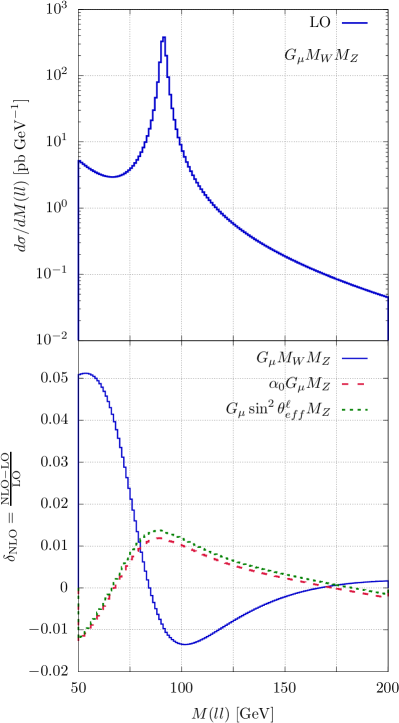
Figure 1: Upper panel: cross section distribution as a function of the leptonic invariant mass, at leading order in the $(G_{\mu},M_{W},M_{Z})$ scheme. Lower panel: relative difference between the NLO cross section and the LO one in the three renormalization schemes $(G_{\mu},M_{W},M_{Z})$ (solid blue), $(\alpha_{0},G_{\mu},M_{Z})$ (dashed red), and $(G_{\mu},\sin^{2}\theta^{\ell}_{eff},M_{Z})$ (dotted green).

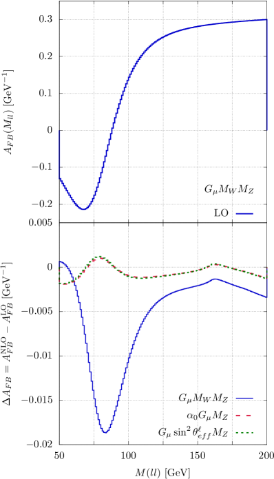
Figure 2: Upper panel: forward-backward asymmetry distribution as a function of the leptonic invariant mass, at leading order in the $(G_{\mu},M_{W},M_{Z})$ scheme. Lower panel: absolute difference between NLO and LO asymmetry in the three renormalization schemes $(G_{\mu},M_{W},M_{Z})$ (solid blue), $(\alpha_{0},G_{\mu},M_{Z})$ (dashed red), and $(G_{\mu},\sin^{2}\theta^{\ell}_{eff},M_{Z})$ (dotted green).

In the Z_ew-BMNNPV package, the choice of leaving $\alpha_{\overline{\rm MS}}(\mu_{0}^{2})$ and $s_{W\,\overline{\rm MS}}^{2}(\mu_{0}^{2})$ as free parameters is motivated by the possibility of measuring $s_{W\,\overline{\rm MS}}^{2}$ at the LHC and future hadron colliders from neutral-current Drell-Yan through a template fit approach, as investigated in Ref. Amoroso:2023uux . Such measurements would require the generation of Monte Carlo templates for different vales of $s_{W\,\overline{\rm MS}}^{2}(\mu_{0}^{2})$ (and possibly $\alpha_{\overline{\rm MS}}(\mu_{0}^{2})$) to be fitted to the data. While the present study is focused on fixed-order results and in particular on weak corrections, the Z_ew-BMNNPV can generate the required templates at NLO QCD+NLO EW accuracy with the consistent matching to QCD and QED parton showers. Another possibility could be to use the $\overline{\rm MS}$ scheme for a precise prediction (rather than determination) of $s_{W}^{2}$ at the weak scale as done in Ref. Degrassi:1990tu ; Degrassi:1990ec ; Sirlin:2012mh ; Degrassi:1996ps ; Gambino:1993dd ; Ferroglia:2002rg ; Ferroglia:2001cr up to full $\mathcal{O}(\alpha)$ accuracy (plus higher order corrections to the running of $\alpha$ and $\Delta\rho$). In this approach $\alpha_{\overline{\rm MS}}(\mu_{0}^{2})$ and $s_{W\,\overline{\rm MS}}^{2}(\mu_{0}^{2})$ are derived quantities computed as functions of other input parameters: typically the calculation is performed in the $(\alpha_{0}$, $G_{\mu}$, $M_{Z})$ scheme given the high accuracy at which these parameters are measured. For what concerns $\alpha_{\overline{\rm MS}}$, it can be computed from $\alpha_{0}$ via the relation

$$\alpha_{\overline{\rm MS}}(\mu^{2})=\frac{\alpha_{0}}{1-\Delta\hat{\alpha}(\mu^{2})},$$ (45)

where $\Delta\hat{\alpha}(\mu^{2})=2[\delta Z_{e}-\delta Z_{e\;\overline{MS}}(\mu^{2})]$ at $\mathcal{O}(\alpha)$ (in the code, leptonic corrections at $\mathcal{O}(\alpha^{2})$ as well as QCD corrections of order $\alpha_{S}$ and $\alpha_{S}^{2}$ are also available). At order $\alpha$, $s_{W\,\overline{\rm MS}}^{2}(\mu^{2})$ can be computed from

$$\sin^{2}\theta_{b}=s_{W\,\overline{\rm MS}}^{2}+\delta s_{W\,\overline{\rm MS}}^{2}=s_{W}^{2}+\delta s_{W}^{2},$$ (46)

where the (renormalized) sine of the weak-mixing angle and the corresponding counterterm at the right-hand side of the second equality are computed in the $(\alpha_{0}$, $G_{\mu}$, $M_{Z})$ scheme. From equation (46) it follows that, at $\mathcal{O}(\alpha)$:

$$s_{W\,\overline{\rm MS}}^{2}(\mu^{2})=s_{W}^{2}+\delta s_{W}^{2}-\delta s_{W\,\overline{\rm MS}}^{2}\pm\delta\sin^{2}\theta_{eff}^{\ell}\,$$ (47)

$$= s_{W}^{2}+\frac{c_{W}^{2}s_{W}^{2}}{c_{W}^{2}-s_{W}^{2}}\Delta\tilde{r}+\delta\sin^{2}\theta_{eff}^{\ell}\,-\delta s_{W\,\overline{\rm MS}}^{2}$$

$$= s_{W}^{2}+\frac{c_{W}^{2}s_{W}^{2}}{c_{W}^{2}-s_{W}^{2}}\Big{[}\Delta r_{\overline{\rm MS}}+2\Big{(}\delta Z_{e}-\delta Z_{e\;\overline{MS}}(\mu^{2})\Big{)}\Big{]},$$

$\Delta r_{\overline{\rm MS}}$ being formally identical to $\Delta\tilde{r}$, but with $\delta Z_{e}$ and $\sin^{2}\theta_{eff}^{\ell}\,$ replaced with $\delta Z_{e\;\overline{MS}}(\mu^{2})$ and $\delta s_{W\,\overline{\rm MS}}^{2}$. As in the case of Eqs. (37) and (38), we can consider Eq. (47) as the NLO expansion of

$$s_{W\,\overline{\rm MS}}^{2}(M_{Z}^{2})=$$

$$\frac{1}{2}-\sqrt{\frac{1}{4}-\frac{\pi\alpha_{0}}{\sqrt{2}G_{\mu}M_{Z}^{2}(1-\Delta\hat{\alpha}(M_{Z}^{2}))}\Big{(}1+\Delta r_{\overline{\rm MS},\,{\rm HO}}\Big{)}}.$$ (48)

In equation (48) the renormalization scale was identified with $M_{Z}^{2}$, given the input-parameter set used, and $\Delta r_{\overline{\rm MS},\,{\rm HO}}$ is obtained from $\Delta r_{\overline{\rm MS}}$ by replacing the $\mathcal{O}(\alpha)$ expression of $\Delta\rho$ with the one including the higher-order corrections discussed in Sect. 3.

A last comment is in order concerning the decoupling procedure. We decouple the top-quark and the $W$ boson in the $\alpha_{\overline{\rm MS}}$ and $s_{W\,\overline{\rm MS}}^{2}$ running to make contact with Refs. Erler:2004in ; Erler:2017knj , mainly motivated by the huge impact of the $W$ decoupling. However we adopt a minimal (and simplified) approach where the top and the $W$ are integrated out only in the renormalization-group equations for $\alpha_{\overline{\rm MS}}$ and $s_{W\,\overline{\rm MS}}^{2}$ and in the expression of the NLO counterterms for $\delta Z_{e\;\overline{MS}}$ and $\delta s_{W\,\overline{\rm MS}}^{2}/s_{W\,\overline{\rm MS}}^{2}$, which are closely related to the evolution equations. The heavy degrees of freedom are not integrated out in the calculation of the relevant matrix elements.

5 Input parameter schemes: numerical results

In this section we investigate the numerical impact of the radiative corrections to differential observables of the NC DY process at the LHC, according to the above described input parameter schemes. In particular, we focus on the dilepton invariant mass distribution $d\sigma/dM_{ll}$ and on the forward-backward asymmetry $A_{\rm FB}(M_{ll})$, defined as:

$$A_{\rm FB}(M_{ll}) = \frac{d\sigma^{F}/dM_{ll}-d\sigma^{B}/dM_{ll}}{d\sigma^{F}/dM_{ll}+d\sigma^{B}/dM_{ll}},$$ (49)

$$d\sigma^{F}/dM_{ll} = \int_{0}^{1}dc\,\frac{d\sigma}{dM_{ll}\,dc}\,,$$ (50)

$$d\sigma^{B}/dM_{ll} = \int_{-1}^{0}dc\,\frac{d\sigma}{dM_{ll}\,dc}\,,$$ (51)

where $c$ is the cosine of the lepton scattering angle in the Collins-Soper frame, as a function of the invariant mass $M_{ll}$. We consider the $\mu^{+}\mu^{-}$ final state, with $\sqrt{s}=13$ TeV. All results are obtained for an inclusive setup, where no cuts are imposed on the final-state leptons except for an invariant mass cut $M_{ll}\geq 50$ GeV. The numerical values of the relevant parameters are specified in A and the default values for the higher order options, for the hadronic contributions to $\Delta\alpha$ as well as for the $W/Z$ boson width options are adopted.

The upper panels of Figs. 1 and 2 show the LO predictions obtained in the $\left(G_{\mu},M_{W},M_{Z}\right)$ scheme for the differential cross section and $A_{FB}$ distribution computed as functions of the dilepton invariant mass $M_{ll}$ in the window $50$ GeV $\leq M_{ll}\leq 200$ GeV, without additional kinematical cuts on the leptons. While the invariant mass distribution has a Breit-Wiegner peak for $M_{ll}$ equal to $Z$ mass, the asymmetry crosses zero and changes sign in the resonance region: because of this behaviour, in the following we quantify the impact of EW corrections or the differences among predictions obtained in different input-parameter schemes in terms of absolute (rather than relative) differences for the $A_{FB}$ distribution.

To analyse the main features of the NLO weak corrections and the higher-order effects discussed in Sects. 3 and 4, we consider the $(\alpha_{0}$, $G_{\mu}$, $M_{Z})$ scheme together with a representative of the class of schemes using $M_{W}$ as independent parameter and a representative for the class using $\sin^{2}\theta_{eff}^{\ell}\,$ as input. We choose schemes with couplings defined at the weak scale, namely $\left(G_{\mu},M_{W},M_{Z}\right)$, $\left(G_{\mu},\sin^{2}\theta_{eff}^{\ell}\,,M_{Z}\right)$, and $(\alpha_{0}$, $G_{\mu}$, $M_{Z})$ with the flag azinscheme4 equal to one (i.e. using $\alpha=\alpha_{0}/(1-\Delta\alpha)$ in the calculation). Other schemes where couplings are defined at low-energy, like the ones involving $\alpha_{0}$, lead to larger corrections with respect to the LO because of the running of the parameters up to the weak scale: such effects tend to reduce the differences w.r.t. to the predictions of schemes relying on $\alpha(M_{Z})$ or $G_{\mu}$ when moving from LO to NLO and NLO+HO accuracy (see Figs. 9-10). In the $\overline{\rm MS}$ scheme of Sect. 4.4, the running of $\alpha_{\overline{\rm MS}}(\mu^{2})$ and $s_{W\,\overline{\rm MS}}^{2}(\mu^{2})$ reabsorbs large part of the corrections in the Born matrix elements: for this reason, the relative corrections with respect to the LO are not shown for the $(\alpha_{\overline{\rm MS}}$, $s_{W\,\overline{\rm MS}}^{2}$, $M_{Z})$ scheme and we only show the $\overline{\rm MS}$ results at NLO with the best predictions (i.e. NLO plus H.O.) in the other schemes (Figs. 9-10).

The lower panel of Fig. 1 shows the NLO relative correction to $d\sigma/dM_{ll}$ w.r.t. the LO prediction, for three input schemes: $(G_{\mu},\sin^{2}\theta_{eff}^{\ell},M_{Z})$ (dotted green line), $\left(\alpha_{0},G_{\mu},M_{Z}\right)$ (dashed red line), and $(G_{\mu},M_{W},M_{Z})$ (solid blue line). The corrections in the first two schemes are very similar, ranging from $-1\%$ to about $+1\%$, with the line corresponding to the $(G_{\mu},\sin^{2}\theta_{eff}^{\ell},M_{Z})$ scheme slightly above the one for the $\left(\alpha_{0},G_{\mu},M_{Z}\right)$ scheme. When using $M_{W}$ as an independent parameter, the corrections have different shape and are in general larger, ranging form $+5\%$ at 40 GeV to $-1\%$ around 100 GeV. The picture could be understood as follows. The analytic expression of the one-loop matrix element in the three schemes is identical once the counterterms are expressed in terms of $\delta Z_{e}$ (or $\delta\tilde{Z}_{e}$) and $\delta s_{W}^{2}$, the only differences being the actual form of the counterterms ($\delta Z_{e}$ and $\delta s_{W}^{2}$) and the $\Delta r$ or $\Delta\tilde{r}$ subtraction terms that factorize on a the tree-level matrix-element in the scheme $(G_{\mu},M_{W},M_{Z})$ or $(G_{\mu},\sin^{2}\theta_{eff}^{\ell},M_{Z})$ schemes, respectively. If one replaces the counterterm $\delta s_{W}^{2}$ with $\delta s_{W}^{2}\pm\delta\sin^{2}\theta_{eff}^{\ell}\,$, one can split the one-loop matrix-element in a term that corresponds to the one-loop amplitude in the scheme $(G_{\mu},\sin^{2}\theta_{eff}^{\ell},M_{Z})$ (up to the above-mentioned subtraction terms which however appear as constant shifts in the relative corrections) plus a reminder that might be written as $\Delta s^{2}_{W}\partial M_{LO}/\partial s^{2}_{W}$ which represents the change in the LO matrix-element when the numerical value of $s^{2}_{W}$ is shifted by a factor $\Delta s^{2}_{W}=\delta s_{W}^{2}-\delta\sin^{2}\theta_{eff}^{\ell}\,$. In the $\left(\alpha_{0},G_{\mu},M_{Z}\right)$ scheme, $\Delta s^{2}_{W}$ is about $2.7\times 10^{-4}$ and the corresponding impact is hardly visible on the scale of the plot, while in the $(G_{\mu},M_{W},M_{Z})$ $\Delta s^{2}_{W}$ is much larger, of order $1\times 10^{-2}$, and it is the main responsible for the shape and the size of the effects shown in Fig. 1. The relative corrections at NLO in the schemes with $\alpha_{0}$ or $\alpha(M_{Z})$ as input together with $M_{W}$ ($\sin^{2}\theta_{eff}^{\ell}\,$) can be obtained from the ones shown in Fig. 1 by removing the constant term $-2\Delta r$ ($-2\Delta\tilde{r}$) or replacing it with $-2\Delta\alpha(M_{Z})$, respectively. The lower panel of Fig. 2 shows the NLO correction to the asymmetry, defined as the absolute difference $\Delta A_{FB}=A_{FB}^{NLO}-A_{FB}^{LO}$. Similarly to what happens for the cross section, the NLO weak corrections with the schemes $(G_{\mu},\sin^{2}\theta_{eff}^{\ell}\,,M_{Z})$ and $\left(\alpha_{0},G_{\mu},M_{Z}\right)$ are very close and in general smaller, falling in the range $\pm 0.002$, while the corrections in the $(G_{\mu},M_{W},M_{Z})$ are larger, reaching the value of $-0.018$ at about 80 GeV. The results for the asymmetry and the ones for the di-lepton invariant mass basically share the same interpretation detailed above, with the main difference that the effect of the overall subtraction terms like $\Delta r$ and $\Delta\tilde{r}$ largely cancel in $A_{FB}^{NLO}$.

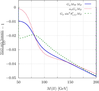
Figure 3: Relative corrections to the invariant mass cross section distribution obtained by considering only NLO bosonic contributions.

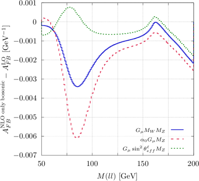
Figure 4: Absolute corrections to the forward-backward asymmetry obtained by considering only NLO bosonic contributions.

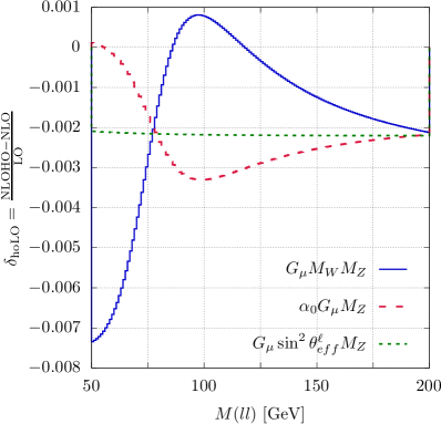
Figure 5: Higher-order correction to the cross section distribution as a function of the leptonic invariant mass. The three curves correspond to the three different choices of renormalization scheme discussed.

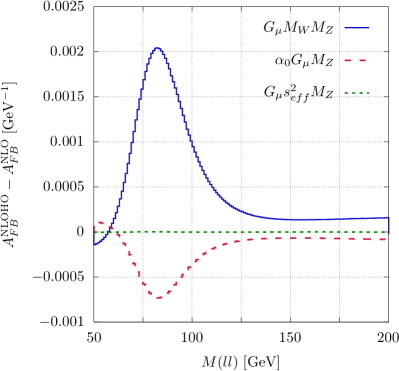
Figure 6: Higher-order correction to the forward-backward asymmetry distribution as a function of the leptonic invariant mass. The three curves correspond to the three different choices of renormalization scheme discussed.

Figures 3 and 4 show the relative (absolute) NLO weak corrections to the cross section (forward -backward asymmetry) if only the gauge-invariant subset of the bosonic loops is included. At low dilepton invariant masses, large part of these corrections come from the bosonic contribution to $\Delta r$ and $\Delta\tilde{r}$ entering the calculation in the $(G_{\mu},M_{W},M_{Z})$ and in the $(G_{\mu},\sin^{2}\theta_{eff}^{\ell},M_{Z})$ schemes, respectively. For larger $M_{ll}$ values, in the right part of the plot, the bosonic corrections are relatively large (order $-5\%$), while the full NLO weak corrections are at the permille level, pointing out a strong cancellation between bosonic and fermionic corrections. The contribution from $\Delta r$ and $\Delta\tilde{r}$ essentially cancels in $A_{FB}$ and the asymmetry difference in Fig. 4 is dominated by the shift induced in the effective $s_{W}^{2}$ by the bosonic part of the $\mathcal{O}(\alpha)$ corrections in the $(\alpha_{0},G_{\mu},M_{Z})$ and $(G_{\mu},M_{W},M_{Z})$ schemes ($\delta s_{W}^{2}\sim 3\times 10^{-3}$ and $\delta s_{W}^{2}\sim 2.5\times 10^{-3}$, respectively). By comparing Figs. 2 and 4, one notices that a large cancellation between bosonic and fermionic effects is still there in the $(\alpha_{0},G_{\mu},M_{Z})$ and $(G_{\mu},M_{W},M_{Z})$ schemes, while in the $(G_{\mu},\sin^{2}\theta_{eff}^{\ell},M_{Z})$ bosonic corrections dominate over the fermionic ones and the lines corresponding to this scheme in Figs. 2 and 4 are almost the same in the scale of the plot.

Figs. 5 and 6 show the higher-order universal corrections (i.e. beyond NLO) defined in Sect. 3, to the cross section invariant mass distribution (normalized to the LO predictions) and the forward-backward asymmetry, respectively, in the three renormalization schemes. As for the NLO case, the plots display the relative corrections for the cross section distribution and the absolute correction for $A_{FB}(M_{ll})$. In the $(G_{\mu},\sin^{2}\theta_{eff}^{\ell},M_{Z})$ scheme the corrections are small (order $0.2\%$) and essentially flat: this is because the corrections in Eq. (24) factorize on the LO matrix-element squared and the only dependence on $M_{ll}$ comes from the running of $\alpha_{S}$ in the QCD corrections to $\Delta\rho$. The corrections in the $(\alpha_{0}$, $G_{\mu}$, $M_{Z})$ scheme fall in the range $[-0.3\%,0]$, being basically zero for low dilepton invariant masses and reaching their maximum around the $Z$-peak: the shape of the corrections is determined by the additional shift $\Delta s_{W}^{HO}$ on top of the NLO one ($\sim 5\times 10^{-5}$) which only affects the $Z$-boson exchange amplitude, while for small invariant masses the dominant contribution is the $\gamma$-exchange. The impact of the fermionic higher-order effects in the $(G_{\mu},M_{W},M_{Z})$ scheme is larger than for the other choices of input parameters, ranging from about $-0.7\%$ at $M_{ll}=50$ GeV to about $+0.1\%$ at the $Z$-peak: in this scheme, the corrections come from the interplay of the shift to $s^{2}_{W}$ ($-9\times 10^{-4}$ in addition to the NLO shift) and the overall factor $2(\Delta\rho-\Delta\rho^{(\alpha)})c_{W}/s_{w}+\Delta\rho^{2}c_{W}^{2}/s_{W}^{2}$ coming from the relation between $\alpha$ and $G_{\mu}$. The latter effect enters also the $\gamma$-exchange diagram and thus affects also the low-invariant mass region of the plot. When considering the asymmetry (Fig. 6), any overall term common to numerator and denominator of Eq. (49) cancels: this is almost the case for the higher-order corrections in the$(G_{\mu},\sin^{2}\theta_{eff}^{\ell},M_{Z})$ scheme, where the factorization of the higher-order terms is only approximate, due to the presence of the NLO corrections, leading to a negligible residual effect of order $10^{-6}$ on the asymmetry difference not visible within the resolution of the plot. The impact in the $(G_{\mu},M_{W},M_{Z})$ scheme is larger, with a maximum of $2\times 10^{-3}$ for $M_{ll}$ around $80$ GeV: the behaviour is essentially determined by the above-mentioned shift in $s_{W}^{2}$ on top of the $\mathcal{O}(\alpha)$ one. In the $(\alpha_{0}$, $G_{\mu}$, $M_{Z})$ scheme the corrections are negative, reaching the value of about $-7\times 10^{-4}$ again at about $80$ GeV, and driven by the higher-order shift on $s_{W}^{2}$.

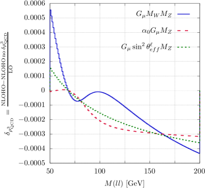
Figure 7: Impact of the three-loop QCD contribution to $\Delta\rho$ on the cross section distribution $d\sigma/dM_{ll}$. The three curves correspond to the three different renormalization schemes.

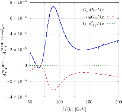
Figure 8: The same as in Fig. 7 for $A_{FB}$. The absolute difference between the three-loop QCD contribution to $\Delta\rho$ and the two-loop case is shown.

Figs. 7 and 8 show the impact of the three-loop QCD correction to $\Delta\rho$, $\delta_{QCD}^{(3)}$ in Eq. 1, normalized to the LO predictions, to the invariant mass cross section distribution and the forward-backward asymmetry, respectively, in the three renormalization schemes. The leading $\delta_{QCD}^{(3)}$ contribution comes from the replacement of the $\Delta\rho^{(\alpha)}$ terms in the NLO calculation with the expression of $\Delta\rho$ in Eq. (1). In the $(G_{\mu}$, $\sin^{2}\theta_{eff}^{\ell}$, $M_{Z})$ scheme, $\Delta\rho$ comes from the relation between $\alpha$ and $G_{\mu}$ and simply multiplies the LO matrix-element squared: the corresponding line in Fig. 7 is twice the factor $3x_{t}(1+x_{t}\Delta\rho^{(2)})\frac{\alpha_{S}^{2}}{\pi^{2}}\delta_{QCD}^{(3)}$ and the dependence on $M_{ll}$ is the residual scale dependence of the QCD correction. In the $(\alpha_{0}$, $G_{\mu}$, $M_{Z})$ scheme, the linear term in $\Delta\rho$ comes from the corrections to the $G_{\mu}M_{Z}^{2}$ factor in the $Z$-boson exchange diagram: as a consequence, in the low dilepton invariant mass region, where the dominant contribution is from $\gamma$-exchange, the correction tends to vanish, while for larger values of $M_{ll}$ it does not factorize on the LO matrix-element. In the $(G_{\mu},M_{W},M_{Z})$ scheme, linear terms in $\Delta\rho$ come both from the $\delta s_{W}^{2}$ counterterm and from the $\Delta r$ relating $\alpha$ and $G_{\mu}$ at NLO ($\sim c_{W}^{2}/s_{W}^{2}\,\Delta\rho$). Only the latter contribution factorizes on the Born result and it is the only one affecting the $\gamma$-exchange which dominates the cross section in the low-invariant mass limit, where the effect is basically three times ($\sim c_{W}^{2}/s_{W}^{2}$) larger than the one observed in the $(G_{\mu}$, $\sin^{2}\theta_{eff}^{\ell}$, $M_{Z})$ scheme. Moving to the asymmetry, the impact of $\delta_{QCD}^{(3)}$ in the $(G_{\mu},\sin^{2}\theta_{eff}^{\ell},M_{Z})$ scheme is not visible in Fig. 8, since it largely cancels between numerator and denominator in $A_{FB}$. Also for the other two schemes the effect is tiny, of the order of $10^{-5}$. The four-loop QCD corrections to $\Delta\rho$ (not included in Z_ew-BMNNPV code) computed at the scale $m_{top}$ should be about five times smaller than the three loop ones Chetyrkin:2006bj , but with reduced scale dependence, so that the numerical impact on the $M_{ll}$ and $A_{FB}$ distributions is negligible compared to the other effects discussed in the following.

We close this subsection presenting in Figs. 9 and 10 the predictions for different schemes referred to the ones obtained in the $(\alpha(M_{Z})$, $\sin^{2}\theta_{eff}^{\ell}$, $M_{Z})$ scheme, for different levels of perturbative accuracy: LO, NLO and NLO with additional universal higher order corrections, named NLOHO, (relative differences for $d\sigma/dM_{ll}$ and absolute differences for $A_{FB}(M_{ll})$). The lower panels, referring to the NLOHO predictions, contain also the results in the hybrid $\overline{\rm MS}$ scheme discussed in Section 4.4, $(\alpha_{\overline{\rm MS}}$, $s_{W\,\overline{\rm MS}}^{2}$, $M_{Z})$. The choice of the reference scheme is motivated by the fact that, in the $(\alpha(M_{Z})$, $\sin^{2}\theta_{eff}^{\ell}$, $M_{Z})$ scheme, the corrections do not involve $\Delta\alpha$- or $\Delta\rho$-enhanced terms and thus the higher-order corrections discussed in Sect. 3 are absent. On the other hand, in the other schemes, the corrections can be split in a non-enhanced part $-$ which is formally the same one as in the $(\alpha(M_{Z})$, $\sin^{2}\theta_{eff}^{\ell}$, $M_{Z})$ scheme with a different numerical value for $\alpha$ and $s_{W}^{2}$ $-$ plus a shift in $s_{W}^{2}$ from Eq. (37) and an overall effect coming from the running of $\alpha$ or from the corrections to the relation between $\alpha$ and $G_{\mu}$ when $\alpha_{0}$ or $G_{\mu}$ are used as input, respectively. When going beyond NLO, the latter effects can have a non-trivial interplay leading, for instance, to mixed contributions of the form $\Delta\alpha\Delta\rho$. As a general comment, the spread of the predictions for the differential cross section based on different input parameter schemes tends to shrink from order $20\%$ per cents at LO to $2\%$ at NLO and few $0.1\%$ with the inclusion of universal additional corrections. The absolute differences for $A_{FB}$ are at the level $0.02$ at LO and become of the order of $10^{-3}$ ($10^{-4}$) when the NLO (NLO plus fermionic higher-order) corrections are included. In the low invariant mass region, dominated by the $\gamma$-exchange diagram, the cross section ratios computed at LO (upper panel of Fig. 9) reduce to ratios of the values of $\alpha$ used in the numerator and in the denominator (squared). For the schemes employing $\alpha(M_{Z})$, including $(\alpha_{0}$, $G_{\mu}$, $M_{Z})$ since the azinscheme4 flag is active, the ratios tend to one at low $M_{ll}$. The same holds for the $(G_{\mu}$, $\sin^{2}\theta_{eff}^{\ell}\,$, $M_{Z})$ scheme, since the value of $\alpha$ computed from $G_{\mu}$ and $\sin^{2}\theta_{eff}^{\ell}\,$ at LO is pretty close to $\alpha(M_{Z})$. For the schemes based on $\alpha_{0}$ the ratios are about $12\%$ smaller, while for the $(G_{\mu}$, $M_{W}$, $M_{Z})$ scheme the corresponding ratio is about $6\%$ smaller than the one for the $\alpha(M_{Z})$-based schemes. At the LO, the only difference in the predictions for the cross section computed in schemes using $\sin^{2}\theta_{eff}^{\ell}\,$ as input comes from the value of $\alpha$ used in the LO couplings: this explains the horizontal lines corresponding to the $(\alpha_{0}$, $\sin^{2}\theta_{eff}^{\ell}\,$, $M_{Z})$ and and $(G_{\mu}$, $\sin^{2}\theta_{eff}^{\ell}\,$, $M_{Z})$ schemes. When using the schemes with $M_{W}$ as input or $(\alpha_{0}$, $G_{\mu}$, $M_{Z})$, not only the value of $\alpha$ used for the couplings changes with respect to the one used in the denominator, but also $s_{W}^{2}$ is different: since a variation of this parameter affects in a different way the $Z$ and $\gamma$-exchange amplitudes (the latter only when $\alpha$ is derived from $G_{\mu}$) which are weighted by the factors $\frac{1}{s-M_{Z}^{2}+i\Gamma_{Z}M_{Z}}$ and $1/s$, respectively, the ratios corresponding to the $M_{W},\sin^{2}\theta_{eff}^{\ell}\,$-based schemes in the upper panel of Fig. 9 have a non trivial shape as a function of $M_{ll}$. For the $(\alpha_{0}$, $G_{\mu}$, $M_{Z})$ scheme, the ratio is still close to one since the value of $s_{W}^{2}$ computed at LO in this scheme is close to the value of $\sin^{2}\theta_{eff}^{\ell}\,$ used in the denominator ($0.2308$ versus $0.2315$, to be compared with $0.2228$ in the $M_{W}$-related schemes). As any overall constant factor cancels between numerator and denominator in $A_{FB}$, the LO asymmetry difference with respect to the $(\alpha(M_{Z})$, $\sin^{2}\theta_{eff}^{\ell}\,$, $M_{Z})$ scheme is zero when $(\alpha_{0}$, $\sin^{2}\theta_{eff}^{\ell}\,$, $M_{Z})$ or $(G_{\mu}$, $\sin^{2}\theta_{eff}^{\ell}\,$, $M_{Z})$ are used as input parameters (upper panel of Fig. 10). For the other schemes one only sees the impact of the different value of $s_{W}^{2}$ used: the three lines for the schemes based on $M_{W}$ overlap, while the one for the $(\alpha_{0}$, $G_{\mu}$, $M_{Z})$ is again closer to the one of the $\sin^{2}\theta_{eff}^{\ell}\,$-based schemes.

At NLO, the spread of the cross section ratios is considerably reduced. In the low $M_{ll}$ region, the ratio stays one for the schemes based on $\alpha(M_{Z})$, while for the $\alpha_{0}$-related schemes it is much closer to one compared to the LO results. This is because the NLO corrections in these schemes develop an overall factor $2\Delta\alpha$ that, once added to the LO term, leads to a sort of LO-improved prediction proportional to the effective coupling $\alpha_{0}^{2}(1+2\Delta\alpha)$ which is just the first-order expansion of $\alpha(M_{Z})^{2}=\alpha_{0}^{2}/(1-\Delta\alpha)^{2}$. Something similar happens for the $(G_{\mu}$, $M_{W}$, $M_{Z})$ scheme including the one-loop corrections to the $\alpha$-$G_{\mu}$ relation contained in $\Delta r$. Besides changing the effective value of $\alpha$ used in the calculation, the one-loop corrections also change the value of the effective $s_{W}^{2}$ used for the $M_{W}$-based and the $(\alpha_{0}$, $G_{\mu}$, $M_{Z})$ schemes: the latter effect is the main responsible for the shape differences in the plots and in particular it explains the change of trend moving from LO to NLO when $M_{W}$ is used as input parameter ($s_{W,\,LO}^{2\,eff}(M_{W})<\sin^{2}\theta_{eff}^{\ell}\,$ while $s_{W,\,NLO}^{2\,eff}(M_{W})>\sin^{2}\theta_{eff}^{\ell}\,$).

Including the higher-order corrections goes in the direction of further reducing the differences among the predictions in different schemes (lower panel of Fig. 9), as this class of corrections is basically obtained in terms of Born-improved matrix elements squared written as functions of effective couplings $\alpha$ and $s_{W}^{2}$ reabsorbing the leading part of the fermionic corrections up to the scale $M_{Z}$ and numerically close to $\alpha(M_{Z})$ and $\sin^{2}\theta_{eff}^{\ell}\,$. It is worth noticing that this sort of redefinition of the couplings in the LO matrix-element does not affect the part of the one-loop result that is not enhanced by large fermionic corrections and in particular does not apply to the bosonic part of the $\mathcal{O}(\alpha)$ result: the different coupling entering this part of the corrections are the main responsible for the residual deviations from one in the lower panel of Fig. 9. As an example, one can take the predictions in the $(\alpha_{0}$, $\sin^{2}\theta_{eff}^{\ell}\,$, $M_{Z})$ scheme: according to Eq. (23), the expression for the NLO+HO corrections is identical to the one in the $(\alpha(M_{Z})$, $\sin^{2}\theta_{eff}^{\ell}\,$, $M_{Z})$ scheme, when $\alpha(M_{Z})$ is obtained from $\alpha_{0}/(1-\Delta\alpha$), and the only difference is the non-enhanced part of the $\mathcal{O}(\alpha)$ result, that is proportional to $\alpha_{0}^{3}$ in the numerator and to $\alpha(M_{Z})^{3}$ in the denominator of the ratio in Fig. 9. This difference alone leads to an effect of order $\pm 0.2\%$ as shown in the plot.

The lower panel of Fig. 9 also shows the ratio of the ${\rm\overline{MS}}$ predictions with respect to the ones in the $(\alpha(M_{Z})$, $\sin^{2}\theta_{eff}^{\ell}\,$, $M_{Z})$ scheme. In the Z_ew-BMNNPV package, we implemented the expressions of Refs. Erler:1998sy and Erler:2004in ; Erler:2017knj for the running of $\alpha_{\overline{\rm MS}}$ and $s_{W\,\overline{\rm MS}}^{2}$ from a scale $\mu_{0}^{2}$ to a scale $\mu^{2}$ leaving both $\mu_{0}^{2}$ and the actual values of $\alpha_{\overline{\rm MS}}(\mu_{0}^{2})$ and $s_{W\,\overline{\rm MS}}^{2}(\mu_{0}^{2})$ as free parameters, since we had in mind the determination of $s_{W\,\overline{\rm MS}}^{2}$ from neutral-current Drell-Yan at the LHC and future hadron-colliders by means of template fits, as in Ref. Amoroso:2023uux : the ${\rm\overline{MS}}$ results thus depend on $\alpha_{\overline{\rm MS}}(\mu_{0}^{2})$ and $s_{W\,\overline{\rm MS}}^{2}(\mu_{0}^{2})$ as input parameters. The solid black line shows the ratio of the ${\rm\overline{MS}}$ prediction over the ones in the $(\alpha(M_{Z})$, $\sin^{2}\theta_{eff}^{\ell}\,$, $M_{Z})$ scheme setting $\alpha_{\overline{\rm MS}}(M_{Z}^{2})$ and $s_{W\,\overline{\rm MS}}^{2}(M_{Z}^{2})$ ($\mu_{0}^{2}=M_{Z}^{2}$) to the values quoted by the PDG Workman:2022ynf (see also A). While the numbers fall in the same ballpark as the ones obtained in the other schemes, the discrepancy tends to be a little larger. The source of the differences is twofold: on the one hand, the values in Ref. Workman:2022ynf are computed with a theoretical accuracy that is not matched by the rest of the calculation in Z_ew-BMNNPV and, on the other hand, the parameters used in their computation and the ones employed in the present study are not tuned. The dashed black line corresponds to the ${\rm\overline{MS}}$ predictions for a tuned choice of $\alpha_{\overline{\rm MS}}(M_{Z}^{2})$ and $s_{W\,\overline{\rm MS}}^{2}(M_{Z}^{2})$: $\alpha_{\overline{\rm MS}}(M_{Z}^{2})$ is consistently computed from $\alpha_{0}$ using the same parameters as in the rest of the calculation, while $s_{W\,\overline{\rm MS}}^{2}(M_{Z}^{2})$ is derived from the input parameters $(\alpha_{0}$, $G_{\mu}$, $M_{Z})$ as described in Sect. 4.4.

The interpretation of Fig. 10 for the asymmetry difference follows closely the one for the dilepton invariant mass cross section distribution, with the main difference that the corrections connected to $\Delta\alpha$ and $\Delta r$ largely cancel between numerator and denominator in $A_{FB}$ (though not exactly, leading for instance to small deviations from zero in the low invariant mass region for the $\sin^{2}\theta_{eff}^{\ell}\,$-based schemes at NLO). and the spread of the predictions in the considered schemes is mainly due to the different values of $s_{W}^{2}$ effectively employed.

The numerical results in Figs. 9–10 are obtained under the assumption that the input parameters are actually free parameters to be set to the corresponding experimental values (or to be used as variables in template fit analyses) and no attempt was made to tune the input parameters for the different schemes (with the only exceptions of $\alpha(M_{Z})$ $-$ computed from $\alpha_{0}$ $-$ and $s_{W\,\overline{\rm MS}}^{2}(\mu_{0}^{2})$ in the tuned $\overline{\rm MS}$ calculation). Another possibility, closer to the strategy used for the numerical predictions for LEP1 studies mentioned in Sect. 4.3, would be to take a reference input scheme, say $(\alpha_{0}$, $G_{\mu}$, $M_{Z})$, and perform the calculation in other schemes, like the $(G_{\mu}$, $M_{W}$, $M_{Z})$, $(G_{\mu}$, $\sin^{2}\theta_{eff}^{\ell}\,$, $M_{Z})$, or $(\alpha_{\overline{\rm MS}}$, $s_{W\,\overline{\rm MS}}^{2}$, $M_{Z})$ ones, but deriving the numerical values of $M_{W}$, $\sin^{2}\theta_{eff}^{\ell}\,$, and $s_{W\,\overline{\rm MS}}^{2}(\mu_{0}^{2})$, from the parameters $\alpha_{0}$, $G_{\mu}$, $M_{Z}^{2}$ using the quantity $\Delta r$ ($\Delta\tilde{r}$) as in Eqs. (39), (41), and (48). Clearly the tuning procedure reduces all the tuned schemes to the reference one at the considered theoretical accuracy (in our case, NLO plus leading fermionic corrections of order $\Delta\alpha^{2}$, $\Delta\rho^{2}$, $\Delta\alpha\Delta\rho$) and it is expected to reduce the spread of the predictions in the peak region (where the tuning is actually performed) but not necessarily away from the resonance. The effect of tuning is shown in Fig. 11 for the dilepton invariant mass cross section distribution (upper panel) and for the forward-backward asymmetry (lower panel), which basically correspond to the lower panels of Figs. 9–10 but taking as reference the $(\alpha_{0}$, $G_{\mu}$, $M_{Z})$ scheme. The maximum spread of the cross section ratios as a function of $M_{ll}$ is of about $0.025$%, while the one for the asymmetry difference is of the order of $0.005$%. As a technical remark, the plots are obtained in the pole scheme in order to minimize the spurious $\mathcal{O}(\alpha^{2})$ effects induced by the CMS, and the fermionic HO corrections in the $(G_{\mu}$, $\sin^{2}\theta_{eff}^{\ell}\,$, $M_{Z})$ scheme are obtained with a modified version of Eq. (24) where $\Delta\rho$ is replaced with $\Delta\tilde{r}$: the expressions are equivalent at the considered theoretical accuracy, differing by terms at most of order $\Delta\tilde{r}_{\rm remn}\Delta\rho$, but this way the effective coupling entering the $Zf\overline{f}$ vertex in the calculation of the fermionic higher-orders in the $(G_{\mu}$, $\sin^{2}\theta_{eff}^{\ell}\,$, $M_{Z})$ and the $(\alpha_{0}$, $G_{\mu}$, $M_{Z})$ schemes become identical.

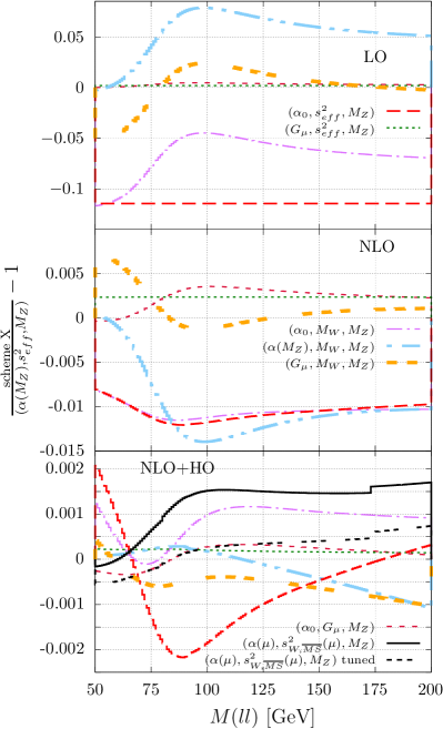
Figure 9: Relative difference of the predictions for the dilepton invariant mass cross section distribution at LO (upper panel), NLO (middle panel), NLO+HO (lower panel). The calculation is performed in the CMS. The $\alpha$ values used in the loop factors corresponds to the one used for the LO couplings. In the $(\alpha_{0}$, $G_{\mu}$, $M_{Z})$ the actual value of $\alpha$ is $\alpha_{0}/(1-\Delta\alpha)$.

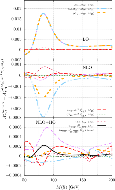
Figure 10: Absolute difference of the predictions for the forward-backward asymmetry as a function of the dilepton invariant mass at LO (upper panel), NLO (middle panel), NLO+HO (lower panel). The calculation is performed in the CMS. The $\alpha$ values used in the loop factors corresponds to the one used for the LO couplings. In the $(\alpha_{0}$, $G_{\mu}$, $M_{Z})$ the actual value of $\alpha$ is $\alpha_{0}/(1-\Delta\alpha)$.

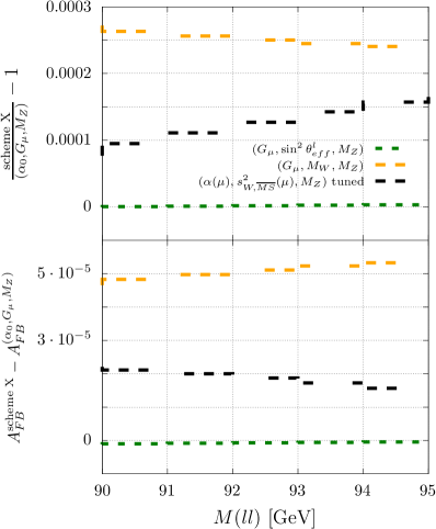
Figure 11: Relative difference (absolute difference) of the predictions for the cross section (forward-backward asymmetry) as a function of the dilepton invariant mass at NLO+HO accuracy. The calculation is performed in the pole scheme. The $\alpha$ values used in the loop factors corresponds to the one used for the LO couplings. In the $(\alpha_{0}$, $G_{\mu}$, $M_{Z})$ the actual value of $\alpha$ is $\alpha_{0}/(1-\Delta\alpha)$. The value of $M_{W}$ used in the $(G_{\mu}$, $M_{W}$, $M_{Z})$ scheme is derived from $(\alpha_{0}$, $G_{\mu}$, $M_{Z})$ using Eq. (39). Similarly, $\sin^{2}\theta_{eff}^{\ell}\,$ and $s_{W\,\overline{\rm MS}}^{2}$ are computed by means of Eqs. (41) and (48).

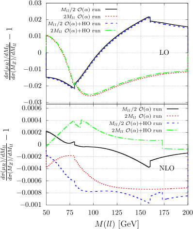
Figure 12: Relative difference of the dilepton invariant mass distribution obtained for $\mu_{R}=2M_{ll}$ (red and green lines) or $\mu_{R}=M_{ll}/2$ (black and blue curves) with respect to the predictions obtained with the default choice $\mu_{R}=M_{ll}$. The $\overline{\rm MS}$ running of $\alpha_{\overline{\rm MS}}(\mu_{R}^{2})$ and $s_{W\,\overline{\rm MS}}^{2}(\mu_{R}^{2})$ is computed at $\mathcal{O}(\alpha)$ in the solid and dotted lines, while in the dashed and dot-dashed lines the running includes the higher-order effects described in the text. The distributions are computed at LO in the upper panel and at NLO in the lower one.

Figure 13: Relative difference between the dilepton invariant mass distributions computed in the $\overline{\rm MS}$ scheme with and without including the HO corrections to the running of $\alpha_{\overline{\rm MS}}(\mu_{R}^{2})$ and $s_{W\,\overline{\rm MS}}^{2}(\mu_{R}^{2})$ described in the main text.

Concerning the $(\alpha_{\overline{\rm MS}}$, $s_{W\,\overline{\rm MS}}^{2}$, $M_{Z})$ scheme, it is interesting to analyze the renormalization-scale dependence of the predictions obtained in this scheme. Fig. 12 shows the ratio of the dilepton invariant mass cross section distribution computed with $\mu_{R}=2M_{ll}$ ($\mu_{R}=M_{ll}/2$) and the one obtained with the default choice $\mu_{R}=M_{ll}$ at LO (upper panel) and NLO (lower panel). Regardless of the accuracy in the matrix element calculation, the running of $\alpha_{\overline{\rm MS}}$ and $s_{W\,\overline{\rm MS}}^{2}$ is computed at $\mathcal{O}(\alpha)$ accuracy (solid and dotted lines) or at $\mathcal{O}(\alpha)$ plus the higher-order corrections taken from Refs. Erler:1998sy ; Erler:2004in ; Erler:2017knj (dashed and dot-dashed lines). In the plots, the finite jumps for $M_{ll}=M_{W}$ ($M_{ll}=2M_{W}$) are a consequence of the discontinuity in the $\mathcal{O}(\alpha)$ running of the $\overline{\rm MS}$ parameters for $\mu_{R}=M_{W}$ at the denominator (at the numerator for the choice $\mu_{R}=M_{ll}/2$). When the HO corrections to the running of $\alpha_{\overline{\rm MS}}$ and $s_{W\,\overline{\rm MS}}^{2}$ are included, similar discontinuities appear also per $M_{ll}=M_{\rm top}$ (and $M_{ll}=2M_{\rm top}$ if $\mu_{R}=M_{ll}/2$). At the LO, scale-variation effects are of order $\pm 2\%$ and the size of the jumps related to the $W$ threshold in the running of the couplings is of about a couple of permille, while the jumps originated by the top threshold in the dashed and dot-dashed lines are not visible on the scale of the plot. In the NLO calculation, the renormalization-scale dependence of $\alpha_{\overline{\rm MS}}$ and $s_{W\,\overline{\rm MS}}^{2}$ cancels against the one of the renormalization counterterms in the one-loop amplitude and the residual scale dependence starts at $\mathcal{O}(\alpha^{2})$. As a consequence, on the one hand scale variation effects are strongly suppressed (compared to the ones in the upper panel) and enter at the sub-permille level and, on the other hand, the jumps at the $W$ threshold are visibly reduced. This does not happen for the discontinuities at the top threshold, since the matching corrections to the running formulae are beyond $\mathcal{O}(\alpha)$. Though the HO corrections to the running of the $\overline{\rm MS}$ parameters are not matched by the $\mathcal{O}(\alpha)$ virtual matrix elements, the size of the renormalization-scale dependence shown by the dashed and dot-dashed lines is close to the one in the solid and dotted plots where only the $\mathcal{O}(\alpha)$ running of $\alpha_{\overline{\rm MS}}$ and $s_{W\,\overline{\rm MS}}^{2}$ is used. It is thus reasonable to take the numerical impact of the HO contribution to the running of the parameters (some $0.01\%$, as shown in Fig. 13) as a rough estimate of the missing higher-order corrections to the matrix elements.

As a general remark, while the difference between theoretical predictions obtained with different input parameter and renormalization schemes can be considered as a rough and conservative estimate of the theoretical control over predictions involving weak corrections, there might be motivations to prefer one scheme to the others, like, for instance, the parametric uncertainties connected with the knowledge of the input parameters, the size of the perturbative corrections, the need of a specific free parameter in the calculation.

In the following we address some of these additional sources of theoretical uncertainty, in particular in Sect. 6 we focus on the main parametric uncertainties, in Sect. 7 we discuss the treatment of the light quark contributions, and in Sect.8 we consider different available strategies for the treatment of the unstable gauge bosons.

6 Parametric uncertainties

We study in the following the parametric uncertainties induced on $d\sigma/d{M_{ll}}$ and $A_{FB}(\mu^{+}\mu^{-})$ by the current experimental errors affecting some of the relevant input parameters for each of the above considered schemes. In particular, we treat the scheme $\left(\alpha_{0},G_{\mu},M_{Z}\right)$ as free from parametric uncertainties due to the input parameters because $\alpha_{0}$, $G_{\mu}$ and $M_{Z}$ are known with excellent accuracy in high energy physics. Therefore, for the other two schemes, $\left(G_{\mu},M_{W},M_{Z}\right)$ and $\left(G_{\mu},\sin^{2}\theta_{eff}^{\ell},M_{Z}\right)$, we study the uncertainties induced by the imperfect knowledge of $M_{W}$ and $\sin^{2}\theta_{eff}^{\ell}$, respectively.

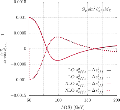
Figure 14: Effects of varying the input parameter $\sin^{2}\theta^{\ell}_{eff}=0.23154\pm 0.00016$ in the $(G_{\mu},\sin^{2}\theta^{\ell}_{eff},M_{Z})$ scheme from the central value to the upper and lower ones, at leading and next-to-leading order. Here it is shown the relative difference between the invariant mass distribution obtained with the upper/lower value of $\sin^{2}\theta^{\ell}_{eff}$ and the one with the central value $\sin^{2}\theta^{\ell}_{eff,c}=0.23154$.

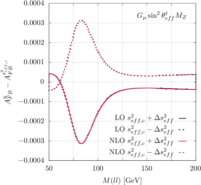
Figure 15: Effects of varying the input parameter $\sin^{2}\theta^{\ell}_{eff}=0.23154\pm 0.00016$ in the $(G_{\mu},\sin^{2}\theta^{\ell}_{eff},M_{Z})$ scheme from the central value to the upper and lower ones, at leading and next-to-leading order. In particular it is shown the absolute difference between the asymmetry distribution obtained with the upper/lower value of $\sin^{2}\theta^{\ell}_{eff}$ and the one with the central value $\sin^{2}\theta^{\ell}_{eff,c}=0.23154$.

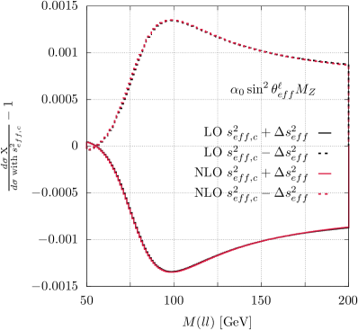
Figure 16: Effects induced on the dilepton invariant mass distribution by a variation of the input parameter $\sin^{2}\theta^{\ell}_{eff}=0.23154\pm 0.00016$ in the $(\alpha_{0},\sin^{2}\theta^{\ell}_{eff},M_{Z})$ scheme from the central value to the upper and lower ones, at leading and next-to-leading order. Same notation and conventions of Fig. 14.

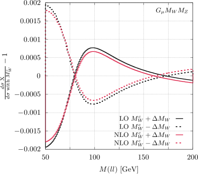
Figure 17: Effects of varying the input parameter $M_{W}=80.385\pm 0.015$ GeV in the $(G_{\mu},M_{W},M_{Z})$ scheme from the central value to the upper and lower ones, at leading and next-to-leading order. Here it is shown the relative difference between the invariant mass distribution obtained with the upper/lower value of $M_{W}$ and the one with the central value $M_{W}^{c}=80.385$ GeV.

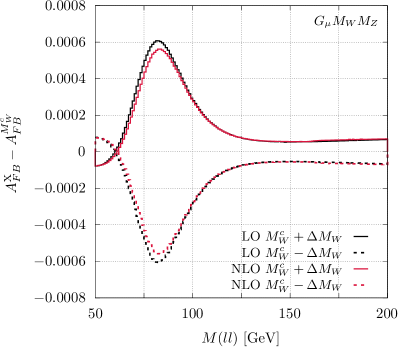
Figure 18: Effects of varying the input parameter $M_{W}=80.385\pm 0.015$ GeV in the $(G_{\mu},M_{W},M_{Z})$ scheme from the central value to the upper and lower ones, at leading and next-to-leading order. In particular it is shown the absolute difference between the asymmetry distribution obtained with the upper/lower value of $M_{W}$ and the one with the central value $M_{W}^{c}=80.385$ GeV.

Figure 14 displays the effect of a variation of $\sin^{2}\theta_{eff}^{\ell}$ within the range $0.23154\pm 0.00016$ ALEPH:2005ab on the dilepton invariant mass distribution computed in the $\left(G_{\mu},\sin^{2}\theta_{eff}^{\ell},M_{Z}\right)$ scheme at LO and NLO accuracy (black and red lines, respectively). In particular, the quantity

$$\delta^{\pm}=\frac{d\sigma}{dM_{ll}^{s^{2}_{\rm eff}\pm\Delta s^{2}_{\rm eff}}}\Big{/}\frac{d\sigma}{dM_{ll}^{s^{2}_{\rm eff}}}-1\,,$$ (52)

where $s^{2}_{\rm eff}$ stands for the reference $\sin^{2}\theta_{eff}^{\ell}$ value ($0.23154$) and $\Delta s^{2}_{\rm eff}=0.00016$, is plotted as a function of $M_{ll}$. Since the renormalization conditions in the $\left(G_{\mu},\sin^{2}\theta_{eff}^{\ell},M_{Z}\right)$ scheme require that $\sin^{2}\theta_{eff}^{\ell}$ is not affected by radiative corrections, the variations of $\sin^{2}\theta_{eff}^{\ell}$ have basically the same impact at LO and at NLO. It is worth noticing that the dependence of $d\sigma/d{M_{ll}}$ on $\sin^{2}\theta_{eff}^{\ell}$ is twofold: on the one hand, it depends on the $g_{V}/g_{A}$ ratio through the $Zf\overline{f}$ vertices and, on the other hand, there is an overall dependence coming from the relation

$$\alpha_{G_{\mu}}=\frac{\sqrt{2}}{\pi}G_{\mu}\sin^{2}\theta_{eff}^{\ell}\left(1-\sin^{2}\theta_{eff}^{\ell}\right)M_{Z}^{2}\,.$$ (53)

The latter effect is the source of the enhancement in the low-mass region of Fig. 14, as can be understood by comparing the predictions in Fig. 14 with the ones in Fig. 16, obtained in the $\left(\alpha_{0},\sin^{2}\theta_{eff}^{\ell},M_{Z}\right)$ scheme. As a consequence, in order to assess the sensitivity of the dilepton invariant mass distribution on the leptonic effective weak mixing angle (considered as a measure of the $g_{V}/g_{A}$ ratio), one should consider the normalized $d\sigma/dM_{ll}$ distribution, rather than the absolute one.

In Figure 15 we plot the quantity

$$\Delta^{\pm}=\frac{dA_{FB}}{dM_{ll}^{s^{2}_{\rm eff}\pm\Delta s^{2}_{\rm eff}}}-\frac{dA_{FB}}{dM_{ll}^{s^{2}_{\rm eff}}}\,,$$ (54)

showing the effects on $dA_{FB}/dM_{ll}$ induced by variations of $\sin^{2}\theta_{eff}^{\ell}$ within the same range considered in Fig. 14. Also in this case, the dependence on $\sin^{2}\theta_{eff}^{\ell}$ is basically the same at LO and at NLO accuracy. Quantitatively, it amounts to approximately $\pm 3\times 10^{-4}$ in the resonance region and drops quickly away from the $Z$ peak. As $A_{FB}$ is defined through a ratio of differential distributions, the overall spurious dependence on $\sin^{2}\theta_{eff}^{\ell}$ related to Eq. (53) cancels and the results in Fig. 15 show the sensitivity of the $A_{FB}$ on the effective leptonic weak-mixing angle.

In Figures 17 and 18, we focus on the parametric uncertainty coming from the value of the $W$-boson mass that affects the predictions obtained in the $(G_{\mu},M_{W},M_{Z})$ scheme. In particular, we plot the quantities in Eqs. (52) and (54) where we replaced $s^{2}_{\rm eff}$ and $\Delta s^{2}_{\rm eff}$ with the reference $W$-mass value ($M_{W}^{c}=80.385$ GeV) and its $1\sigma$ error ($\Delta M_{W}=\pm 15$ MeV ). Figures 17 (18) and 14 (15) are very similar. This can be understood for instance at LO, where the variations of $M_{W}$ and $\sin^{2}\theta_{eff}^{\ell}$ are related by

$$\delta\sin^{2}\theta_{eff}^{\ell}=-2\left(\frac{M_{W}}{M_{Z}^{2}}\right)\delta M_{W}\,,$$ (55)

from which we can see that a shift of $15$ MeV in $M_{W}$ corresponds to a shift of $-0.0003$ in $\sin^{2}\theta_{eff}^{\ell}$, which is approximately twice the shift we are considering in Figs. 14 and 15. The plots show the same pattern also at NLO, though the relation between $\sin^{2}\theta_{eff}^{\ell}$ and $M_{W}$ beyond LO is more involved (indeed, at variance with the plots in Figs. 14 and 15, in Figs. 17 and 18 the NLO curves do not overlap with the LO ones). As in the case of Fig. 14, the source of the enhancement in the low invariant mass region of Fig. 17 is the overall dependence on $M_{W}$ originating from the relation

$$\alpha_{G_{\mu}}=\frac{\sqrt{2}}{\pi}G_{\mu}M_{W}^{2}\Big{(}1-\frac{M_{W}^{2}}{M_{Z}^{2}}\Big{)}\,,$$ (56)

where the real part of the masses is taken in the complex-mass scheme.

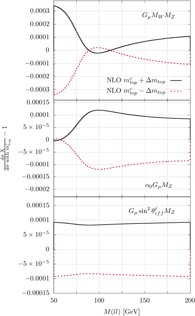
Figure 19: Effects of varying the top-quark mass $m_{top}=173.0\pm 0.4$ GeV in the three considered schemes, from the central value to the upper and lower ones. The top-quark mass enters only the next-to-leading order corrections. Here it is shown the relative difference between the invariant mass distribution obtained with the upper/lower value of $m_{top}$ and the one with the central value $m_{top}^{c}=173.0$ GeV.

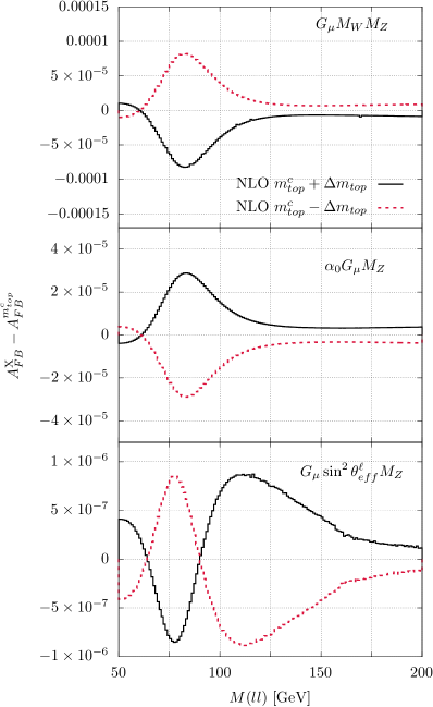
Figure 20: Effects of varying the top-quark mass $m_{top}=173.0\pm 0.4$ GeV in the three considered schemes, from the central value to the upper and lower ones. The top-quark mass enters only the NLO corrections. Here it is shown the absolute difference between the asymmetry distribution obtained with the upper/lower value of $m_{top}$ and the one with the central value $m_{top}^{c}=173.0$ GeV.

Figs. 19 and 20 show the sensitivity of $d\sigma/dM_{ll}$ and $dA_{FB}/dM_{ll}$ to variations of $400$ MeV  in the top-quark mass value, for the three different input parameter schemes. Since $m_{\rm top}$ enters parametrically only through the loop diagrams, we display only the results obtained with the NLO predictions. The largest part of the top–quark mass dependence at $\mathcal{O}(\alpha)$ can be encoded in the $\Delta\rho$ factor defined in Sect. 3. In the NLO predictions computed in the $(G_{\mu}$, $M_{W}$, $M_{Z})$ scheme, $\Delta\rho$ enters in two different ways: through the overall factor $-2\Delta r$ ($\sim 2c_{W}^{2}/s_{W}^{2}$) and via the counterterm corresponding to $s_{W}^{2}$ ($\delta s_{W}^{2}\sim c_{W}^{2}\Delta\rho$). The former contribution is responsible for the constant shift of about $\pm 3\times 10^{-4}$ for $\Delta m_{top}=\pm 0.4$ GeV clearly visible at low dilepton invariant masses, while the latter is the source of the shape effect in the upper panel of Fig. 19. In the $(\alpha_{0}$, $G_{\mu}$, $M_{Z})$ scheme, $\Delta\rho$ enters the $\mathcal{O}(\alpha)$ predictions only via the counterterms $\delta G_{\mu}$ and $\delta s_{W}^{2}$: as a consequence, the $\gamma$-exchange amplitude is not affected by top-mass variations, as clearly visible in the low dilepton invariant-mass region in the central panel of Fig. 19. In the $(G_{\mu}$, $\sin^{2}\theta_{eff}^{\ell}\,$, $M_{Z})$ scheme, $\Delta\rho$ comes from the overall factor $-2\Delta\tilde{r}$ ($\sim 2\Delta\rho$) and induces a constant shift approximately three times smaller than the one coming from $\Delta r$ in the $(G_{\mu}$, $M_{W}$, $M_{Z})$ scheme (given the different coefficients multiplying $\Delta\rho$ in the two calculations, namely $c_{W}^{2}/s_{W}^{2}$ and $1$). The two lines in the lower panel of Fig. 19 are not completely flat because, besides the quadratic terms in $m_{\rm top}$ collected in $\Delta\rho$, there is a residual subleading dependence on the top-quark mass which leads to a tiny relative effect of order $10^{-6}$. In the forward-backward asymmetry the overall contributions from $\Delta r$ and $\Delta\tilde{r}$ largely cancel. As a result, Fig. 20 shows the impact of the $\Delta\rho$ term in $\delta s_{W}^{2}$ (which, in turn, is a shift of the effective $s_{W}^{2}$ entering the calculation) for the $(G_{\mu}$, $M_{W}$, $M_{Z})$ and $(\alpha_{0}$, $G_{\mu}$, $M_{Z})$ schemes, while for the $(G_{\mu}$, $\sin^{2}\theta_{eff}^{\ell}\,$, $M_{Z})$ scheme we only see the impact of the non-enhanced $m_{\rm top}$ corrections which is basically two orders of magnitude smaller than the effect observed for the other schemes.

7 Treatment of $\Delta\alpha^{\rm had}$

The contributions to the running of $\alpha$ coming from the charged leptons and the top quark can be computed perturbatively in terms of the corresponding contributions to the photon self-energy and its derivative, namely:

$$\Delta\alpha^{\rm lept\,(top)}(q^{2})=-\frac{{\rm Re}\Sigma_{AA}^{\rm lept\,(top)}(q^{2})}{q^{2}}+\frac{\partial\Sigma_{AA}^{\rm lept\,(top)}(q^{2})}{\partial q^{2}}\Big{|}_{q^{2}=0}.$$ (57)

For the light-quark contributions, on the contrary, Eq. (57) cannot be used because of the ambiguities related to the definition of the light-quark masses arising from non-perturbative QCD effects. In the literature, a common strategy to compute the light-quark contribution to $\Delta\alpha$ is the introduction of light fermion masses as effective parameters which are used to calculate the analogous of Eq. (57) for the quark sector:

$$\Delta\alpha^{\rm had\,pert.}(q^{2})=-\frac{{\rm Re}\Sigma_{AA}^{\rm had}(q^{2})}{q^{2}}+\frac{\partial\Sigma_{AA}^{\rm had}(q^{2})}{\partial q^{2}}\Big{|}_{q^{2}=0}.$$ (58)

The light-quark masses are chosen is such a way that the resulting hadronic running of $\alpha$ from 0 to $M_{Z}^{2}$ corresponds to the one obtained from the experimental results for inclusive hadron production in $e^{+}e^{-}$ collisions using dispersion relations ($\Delta\alpha^{\rm had\,fit}$), namely:

$$\Delta\alpha^{\rm had\,pert.}(M_{Z}^{2})=\Delta\alpha^{\rm had\,fit}(M_{Z}^{2}).$$ (59)

This approach is implemented in Z_ew-BMNNPV and it is used as a default. We stress that the light-quark masses are only used for the self-energy corrections but they do not enter the vertex and box diagrams. In particular, they are not used for the QED corrections, where the light-quarks mass singularities are regularized by means of dimensional regularization.

Starting from revision 4047, a more accurate treatment of the hadronic vacuum polarization is available in Z_ew-BMNNPV. The code contains an interface to the routines of Refs. Jegerlehner:1985gq ; Burkhardt:1989ky ; Eidelman:1995ny ; Jegerlehner:2003rx ; Jegerlehner:2006ju ; Jegerlehner:2008rs ; Jegerlehner:2011mw ; Jegerlehner:2019lxt and Hagiwara:2003da ; Hagiwara:2006jt ; Hagiwara:2011af ; Keshavarzi:2018mgv (HADR5X19.F and KNT v3.0.1, respectively) for the calculation of the hadronic running of $\alpha$ based on the experimental data for inclusive $e^{+}e^{-}\to$ hadron production at low energies in terms of dispersion relations. This interface can be activated using the input flag da_had_from_fit=1 and the flag fit=1,2 can be used to switch between the two routines for $\Delta\alpha^{\rm had\,fit}$. It is worth noticing that these routines only provide results in the range $[0,q^{2}_{\rm max}]$: for larger values of $q^{2}$, we define

$$\Delta\alpha^{\rm had\,fit} ( q^{2})=\Delta\alpha^{\rm had\,fit}(q^{2}_{\rm max})$$ (60)

$$+ \Delta\alpha^{\rm had\,pert.}(q^{2})-\Delta\alpha^{\rm had\,pert.}(q^{2}_{\rm max}).$$

The starting point for the calculation for da_had_from_fit=1 is the relation

$$\Delta\alpha^{\rm had\,fit}(q^{2})=-\frac{{\rm Re}\Sigma_{AA}^{\rm had}(q^{2})}{q^{2}}+\frac{\partial\Sigma_{AA}^{\rm had\,fit}(q^{2})}{\partial q^{2}}\Big{|}_{q^{2}=0}.$$ (61)

While Eq. (58) is a definition of $\Delta\alpha^{\rm had\,pert.}$, Eq. (61) can be considered as a definition of $\frac{\partial\Sigma_{AA}^{\rm had\,fit}(q^{2})}{\partial q^{2}}\Big{|}_{q^{2}=0}$. On the one hand, Eq. (61) is used in the one-loop corrections to the photon propagator to replace the combination $\Sigma_{AA}^{\rm had}(s)-s\delta Z_{A}^{\rm had}$ with $-s\Delta\alpha^{\rm had\,fit}(q^{2})+is{\rm Im}\Sigma_{AA}^{\rm had}(s)$ (where the factor $\delta Z_{A}^{\rm had}=$ $-\frac{\partial\Sigma_{AA}^{\rm had}(q^{2})}{\partial q^{2}}\Big{|}_{q^{2}=0}$ is the light-quark contribution to the photon wave function renormalization counterterm) and, on the other hand, $\frac{\partial\Sigma_{AA}^{\rm had\,fit}(q^{2})}{\partial q^{2}}\Big{|}_{q^{2}=0}$ is used for the counterterms related to the electric charge and the photon wave function. More precisely, since the self-energy in Eq. (61) can be computed perturbatively for $q^{2}$ much larger than $\Lambda^{2}_{\rm QCD}$, we take $q^{2}=M^{2}_{Z}$ and tune the quark masses using Eq. (59). This way, the formal expression of the counterterms is the same as the one used in the default computation (da_had_from_fit=0). The calculations for da_had_from_fit set to 0 and 1 are not equivalent: in fact, even though both of them rely on the tuning of the light-quark masses from Eq. (59), the corrections to the photon propagator are different since $\Delta\alpha^{\rm had\,fit}(s)\neq\Delta\alpha^{\rm had\,pert.}(s)$ for $s\neq M_{Z}^{2}$.

We notice that the electric-charge and wave function counterterms could also be defined from Eq. (61) setting the light-quark masses to zero in the photon self-energy diagrams: on the one hand, this would lead to differences of order $\alpha\left(\frac{m_{q}^{2}}{M_{Z}^{2}}\right){\rm log}\left(\frac{m_{q}^{2}}{M_{Z}^{2}}\right)$ and, on the other hand, setting the light-quark masses to zero would require several modifications to the routines used for the evaluation of the virtual one-loop corrections.

The impact of the improved treatment of the hadronic running of $\alpha$ is only visible for the input parameter schemes that use $\alpha_{0}$ as an independent parameter, since for the other schemes the terms that depend logarithmically on the light-quark masses cancel. Fig. 21 shows the dependence of $d\sigma/dM_{ll}$ on the uncertainty $\delta\Delta\alpha^{\rm had\,fit}$ for each of the two adopted parameterizations, with the $(\alpha_{0},M_{W},M_{Z})$ scheme. The effect of changing $\Delta\alpha^{\rm had}$ from its central value by a shift of $\pm\delta\Delta\alpha^{\rm had}$ is at the level of $\pm 0.022$% for HADR5X19.F and $\pm 0.027$% for KNT v3.0.1, respectively. Variations of $\Delta\alpha^{\rm had}$ mainly affect the $\delta Z_{e}$ counterterm, as the light-quark mass logarithms in $\delta Z_{e}$ have been traded for $\Delta\alpha^{\rm had}$, leading to an almost constant shift in Fig. 21. Changing $\Delta\alpha^{\rm had}$ also affects the NLO corrected $\gamma$ propagator, but the numerical impact is tiny as the bare self-energy diagrams do not involve logarithmically enhanced light-quark mass terms: this effect, being only present for the $\gamma$-mediated amplitude, induces a small shape effect in Fig. 21. In $A_{FB}$ the contribution from $\delta Z_{e}$ largely cancels, leading to an absolute change in $A_{FB}$ at the $10^{-6}$ level as shown in Fig. 22.

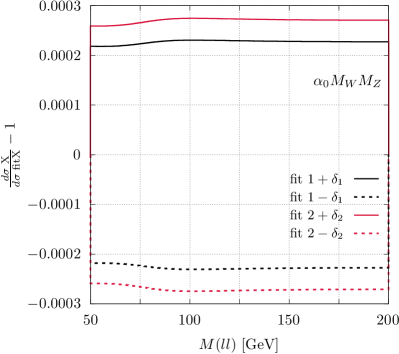
Figure 21: Change in the cross section as a function of the invariant mass if one takes the central value for $\Delta\alpha^{\rm had\,fit}$ (that here coincides with zero) plus its error $\delta\Delta\alpha^{\rm had\,fit}$, here labelled $\delta_{1}$ for results obtained with the flag fit=1 Jegerlehner:1985gq ; Burkhardt:1989ky ; Eidelman:1995ny ; Jegerlehner:2003rx ; Jegerlehner:2006ju ; Jegerlehner:2008rs ; Jegerlehner:2011mw ; Jegerlehner:2019lxt , and $\delta_{2}$ for results with the flag fit=2 Hagiwara:2003da ; Hagiwara:2006jt ; Hagiwara:2011af ; Keshavarzi:2018mgv . The input scheme used here is $(\alpha_{0},M_{W},M_{Z})$.

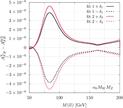
Figure 22: Change in the asymmetry distribution if one takes the central value for $\Delta\alpha^{\rm had\,fit}$ plus its uncertainty $\delta\Delta\alpha^{\rm had\,fit}$, as in Fig. 21.

8 Treatment of the $Z$ width

The unstable nature of the $Z$ vector boson is considered by default through the complex-mass scheme (CMS) Denner:1999gp ; Denner:2005fg ; Denner:2006ic , according to which the squared vector boson masses are taken as complex quantities $\mu^{2}_{V}=M^{2}_{V}-i\Gamma_{V}M_{V}$, with $(V=W,Z)$, in the LO and NLO calculation. The input values for $M_{V}$ and $\Gamma_{V}$ are assumed to be the on-shell ones, $M_{V}^{\rm OS}$ and $\Gamma_{V}^{\rm OS}$, and are converted internally in the initialization phase to the corresponding pole values using the relations Bardin:1988xt ; Beenakker:1996kn

$$M_{V}=\frac{M_{V}^{\rm OS}}{\sqrt{1+\Big{(}\frac{\Gamma_{V}^{\rm OS}}{M_{V}^{\rm OS}}\Big{)}^{2}}},\quad\Gamma_{V}=\frac{\Gamma_{V}^{\rm OS}}{\sqrt{1+\Big{(}\frac{\Gamma_{V}^{\rm OS}}{M_{V}^{\rm OS}}\Big{)}^{2}}}.$$ (62)

The pole parameters $M_{V}$ and $\Gamma_{V}$ are used throughout the code for the matrix element calculations. In the CMS, the couplings that are functions of the gauge-boson masses become necessarily complex quantities. In particular, in the schemes with $M_{W}$ and $M_{Z}$ as input parameters, the quantities $s_{W}^{2}$ and $\delta s_{W}/s_{W}$ of Eq. (5) and Eq. (6) are calculated in terms of $\mu_{W}$ and $\mu_{Z}$. Since $\sin^{2}\theta_{eff}^{\ell}$ is defined through the real part of the $g_{V}/g_{A}$ ratio, it is considered as a real quantity when used as a free parameter. Similarly, the input parameters $\alpha_{0}$, $\alpha(M_{Z})$, and $G_{\mu}$ are real. As a consequence, in the input parameter schemes with only one vector boson mass, $M_{Z}$, the input couplings are taken as real quantities.

When performing calculations in the input parameter/ renormalization schemes having $G_{\mu}$ among the free parameters (with the only exception of the $(\alpha_{0}$,$G_{\mu}$,$M_{Z})$ one), $G_{\mu}$ is usually traded for $\alpha_{G_{\mu}}$ by means of Eqs. (53) or (56). Since the gauge-boson masses enter in this relations, $\alpha_{G_{\mu}}$ might in principle acquire an imaginary part if the CMS scheme is employed. In the code, we follow the standard procedure of taking a real-valued $\alpha_{G_{\mu}}$ to minimize the spurious higher-order terms associated with the overall factor $({\rm Im\alpha_{G_{\mu}}})^{2}$. More precisely, in Eqs. (53) in (56), we always use the real part of the gauge-boson masses.

The CMS preserves gauge invariance order by order in perturbation theory and this feature guarantees also that the higher-order unitarity violations are not artificially enhanced. For this reason it is the scheme commonly adopted for multi-particle NLO calculations. However, for neutral-current Drell-Yan it is possible to adopt other strategies for the treatment of the $Z$ resonance. In particular, in the Z_ew-BMNNPV package, we implemented the so-called pole and factorization schemes following Secs. 3.3.ii and 3.3.iii of Ref. Dittmaier:2009cr , respectively . These schemes can be switched on by means of the flags PS_scheme 1 and FS_scheme 1, respectively.

In Figs. 23 we show the relative difference between the pole (factorization) scheme, blue (red) line, w.r.t. the CMS, for $d\sigma/dM_{ll}$, considering different input parameter schemes. A feature common to all schemes is the oscillation of few 0.01% of amplitude around the $Z$ resonance, as already shown separately for $u{\bar{u}}$ and $d{\bar{d}}$ partonic initial states in Ref. Dittmaier:2009cr . Over the whole range $50$ GeV $<M_{ll}<200$ GeV, the shapes of the differences are similar for the three considered input parameter schemes, with larger differences appearing with the $(G_{\mu},\mbox{$M_{W}$},M_{Z})$ and $(\alpha_{0},G_{\mu},M_{Z})$ schemes. The structure at the $WW$ threshold present in Fig. 6 of Ref. Dittmaier:2009cr is not visible, within the available statistical error, because of a partial cancellation between the contributions of up- and down-type quark channels.

The same comparison between pole (factorization) scheme and CMS is shown for $A_{FB}$ as a function of $M_{ll}$ in Fig. 24. In this case we plot the absolute difference instead of the relative difference with respect to the CMS. For $A_{FB}$ the difference is smooth around the $Z$ resonance, being of the order of few 0.001% for the pole scheme and of the order of 0.01% for the factorization scheme. Contrary to the $d\sigma/dM_{ll}$ case, in Fig 24 the $WW$ threshold enhancement, of the order of 0.05%, is clearly visible.

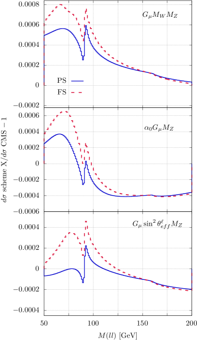
Figure 23: Difference of the pole/factorization scheme with respect to the default complex-mass scheme in the dilepton invariant mass cross section distribution at NLO. The difference PS-CMS is shown by the solid blue curve, the FS-CMS one by the dashed red one. Upper panel: $(G_{\mu},M_{W},M_{Z})$; middle panel: $(\alpha_{0},G_{\mu},M_{Z})$; lower panel: $(G_{\mu},\sin^{2}\theta_{eff}^{\ell},M_{Z})$.

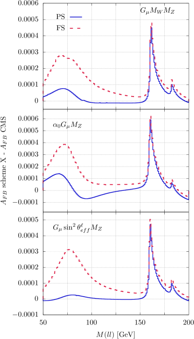
Figure 24: Difference of the pole/factorization scheme with respect to the default complex-mass scheme in the forward-backward asymmetry distribution at NLO. The difference PS-CMS is shown by the solid blue curve, while the FS-CMS one by the dashed red one. Upper panel: $(G_{\mu},M_{W},M_{Z})$; middle panel: $(\alpha_{0},G_{\mu},M_{Z})$; lower panel: $(G_{\mu},\sin^{2}\theta_{eff}^{\ell},M_{Z})$.

9 High energy regime

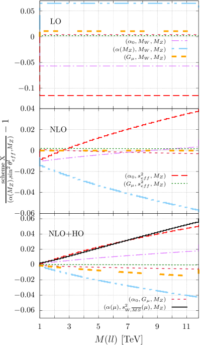
Figure 25: Relative difference of the predictions for the dilepton invariant mass cross section distribution at LO (upper panel), NLO (middle panel), NLO+HO (lower panel), in the range $1-12$ TeV. The calculation is performed with the same inputs of Fig. 9.

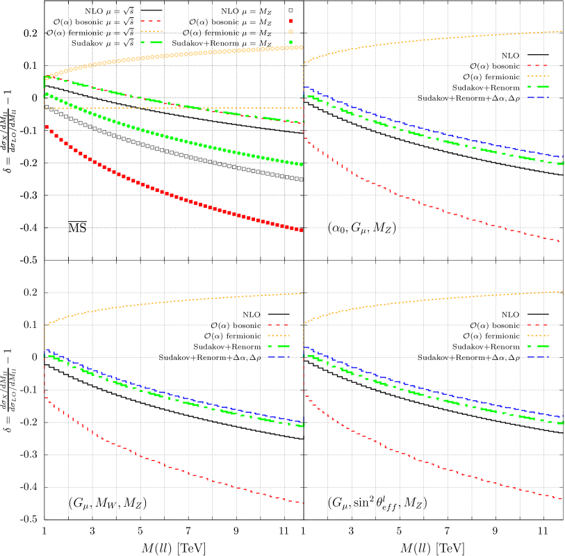
Figure 26: Comparison among the predictions for the dilepton invariant mass cross section distribution, obtained by including the full NLO weak corrections, the fermionic-only and bosonic-only corrections, or the approximation which includes the Sudakov logarithms, the parameter-renormalization logs and the leading fermionic corrections stemming from $\Delta\alpha$ and $\Delta\rho$. Four schemes are shown: the $\overline{\rm MS}$ in both its running- and fixed-scale realizations, the latter one with $\mu=\mbox{$M_{Z}$}$ (top left), $(\alpha_{0},G_{\mu},\mbox{$M_{Z}$})$ (top right), $(G_{\mu},\mbox{$M_{W}$},\mbox{$M_{Z}$})$ (bottom left) and $(G_{\mu},\sin^{2}\theta_{eff}^{\ell}\,,\mbox{$M_{Z}$})$ (bottom right).

The analysis presented so far has been focused on the physics at the $Z$ peak. To complete this study, we examine now the behaviour of the corrections and the interplay among different renormalization and input schemes in the high-energy regime, that can be relevant also in view of the upcoming programme of the LHC and at future high-energy machines.

In this section, we present the results for a specific initial-state quark flavour focusing, for brevity, on $d$-quarks: in this way PDFs contributions exactly cancel when studying the relative effect of weak corrections with respect to the LO, as well as in the ratio of predictions obtained for different schemes. The main motivation of our choice is the fact that, at high dilepton invariant masses, PDFs are poorly constrained and typically affected by large errors. If one considers the contribution of all quark flavors at the same time, the above-mentioned relative corrections and ratios have a residual dependence on PDFs which tends to induce, for high $M_{ll}$ values, quite large unphysical distortions. The actual size of this effect clearly depends on the specific PDF set used.

In Fig. 25 we repeat the study in Fig. 9 for dilepton invariant masses in the range between 1 and 12 TeV. With respect to the peak region, we find a quite different behaviour. First of all, the dilepton invariant mass ratios at LO are flat. In the upper panel of Fig. 9, the shapes came from the variations in the values of $s_{W}^{2}$ entering the $g_{Zf\overline{f}}$ couplings in the $Z$-boson exchange diagram and the $M_{ll}$ dependence was originated by the different propagators of the $\gamma$ and the $Z$ as well as by PDFs weighting the different quark flavours: in Fig. 25 not only we consider only $d$-quarks, but also the $Z$-boson propagator is effectively $1/s$ (since $s\gg M_{Z}^{2}$) so that the only $s$ dependence in the differential cross section is the overall flux factor (see for instance Eq. (2.12) of Dittmaier:2009cr with $\chi_{Z}=1$.)

Moving to the NLO results, the level of agreement between the different input parameter/renormalization schemes is of the order of 1% at the left edge of the plot, but it gets worse as the partonic center of mass energy increases, with a 10% spread at 12 TeV. The inclusion of the fermionic higher-order effects discussed in the previous sections improves the picture only around 1 TeV, but it does not reabsorb the differences among the predictions in the considered schemes at large $M_{ll}$.

The behaviour shown in Fig. 25 can be understood as follows. In the considered dilepton invariant mass range, the bosonic part of the weak NLO corrections is dominated by the so-called Sudakov logarithms, which are double and single logarithms of kinematic invariants over the gauge-boson masses. These logs correspond to the infrared limit of the weak corrections, where the gauge-boson masses are small compared to the energy scales involved and act as (physical) cutoff for the soft and/or collinear virtual weak corrections Sudakov:1954sw ; Beccaria:1998qe ; Ciafaloni:1998xg ; Beccaria:1999fk ; Denner:2000jv ; Denner:2001gw ; Pozzorini:2001rs ; Denner:2003wi ; Denner:2004iz ; Denner:2006jr ; Denner:2008yn ; Fadin:1999bq ; Ciafaloni:1999ub ; Ciafaloni:2000df ; Ciafaloni:2000rp ; Ciafaloni:2000gm ; Ciafaloni:2001vt ; Ciafaloni:2001vu ; Chiu:2007yn ; Chiu:2007dg ; Chiu:2008vv ; Chiu:2009mg ; Becher:2013zua ; Manohar:2014vxa ; Bauer:2017bnh . Besides the Sudakov corrections, there is another class of logarithmic corrections coming from parameter renormalization. When using dimensional regularization, counterterms contain logarithms of the unphysical mass-dimension scale $\mu_{D}$ in the combination

$$\frac{1}{\epsilon}-\log\frac{r_{ct}^{2}}{\mu_{D}^{2}}\,,$$ (63)

where $\epsilon=(4-D)/2$, $D$ being the number of space-time dimensions, and $r_{ct}$ is related to particle masses in on-shell based schemes or directly to the renormalization scale $\mu_{R}$ in the ${\rm\overline{MS}}$ scheme. This contribution cancels against similar terms appearing in the bare loop diagrams (where $r_{ct}$ will be some other scale, say $r_{bare}$) leaving contribution of the form $\log(r_{bare}^{2}/r_{ct}^{2})$. In the Drell-Yan parameter-renormalization counterterms only vertex diagrams enter, so the only possible scale (in particular in the limit of vanishing gauge-boson masses) is $M_{ll}$. The functional form of both the Sudakov and the parameter-renormalization logarithms is the same in any scheme, but the coefficients multiplying the logarithms (including the LO-like amplitude where they appear and the LO amplitude in interference with it) differ numerically as they are function of the actual $\alpha$ and $s_{W}^{2}$ values used. As a result, the logarithms appearing at numerator and denominator in the NLO ratios of Fig. 25 have different coefficients and they do not cancel, leaving logarithmically enhanced remnants. It is worth emphasising that the inclusion of the fermionic higher-order corrections, by definition has no impact on the Sudakov corrections (as they are bosonic), but they are also irrelevant for the parameter-renormalization logs as the corrections in Sect. 3 do include an effective running of the parameters, but only up to the weak scale.

In order to prove the argument above, we implemented a private version of the Z_ew-BMMNPV including the routines used in Chiesa:2013yma ; Mangano:2016jyj for the evaluation of the Sudakov corrections in ALPGEN Mangano:2002ea . Though it is true that the Sudakov corrections alone are not a good approximation for the full NLO weak corrections to neutral-current Drell-Yan (as pointed-out, for instance, in Denner:2019vbn ), this is mainly due to the large cancellations between fermionic and bosonic corrections (as shown in Fig. 26) and to a large UV contribution from parameter-renormalization logarithms. For the on-shell renormalization based schemes, like the $(\alpha_{0},G_{\mu},M_{Z})$, $(G_{\mu},\sin^{2}\theta_{eff}^{\ell},M_{Z})$, and $(G_{\mu},M_{W},M_{Z})$ shown in the plot, the fermionic $\mathcal{O}(\alpha)$ corrections are of the order of $10-20\%$ and mainly come from the fermionic loops entering parameter renormalization. The sum of the Sudakov corrections and the logarithms from parameter renormalization is a reasonable approximation of the NLO corrections, reproducing their shape with an essentially constant shift of about $5-6\%$. Similar consideration apply to the $\overline{\rm MS}$ scheme, if fixed renormalization scale is used ($\mu_{R}=M_{Z}$ in Fig. 26). The picture changes considerably if the $\overline{\rm MS}$ scheme is used with the renormalization scale set to the dilepton invariant mass: in this way, the corrections related to parameter renormalization are reabsorbed in the running couplings and the remaining corrections are smaller than in the other schemes (the fermionic ones, in particular, boil-down to an almost flat $-4\%$ effect). The figure also singles-out the part of the fermionic contributions coming from the universal enhanced terms $\Delta\alpha$ and $\Delta\rho$.

To conclude, in Fig. 27 we repeat the same study of the lower panel of Fig. 25 once the leading logarithmic corrections (Sudakov plus parameter-renormalization logs) have been subtracted from the NLO+HO predictions. Despite the approximations in the calculation of the logarithmic corrections, it is still possible to read a clear trend in Fig. 27: the ratios fall in the few per mille range (as in the case of Fig. 9 for the near-resonance region) and they tend to be flat.

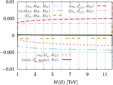
Figure 27: Relative difference of the predictions for the dilepton invariant mass cross section distribution at NLO+HO, after the subtraction of the leading logarithmic corrections (Sudakov plus parameter-renormalization logs).

As thoroughly discussed in the literature, when electroweak Sudakov logarithms start to become dominant a resummation algorithm needs to be adopted, in order to obtain reliable predictions. A very recent discussion on automated resummation algorithms of Sudakov logarithms in simulation tools can be found in Ref. Denner:2024yut . This issue is left to future investigations for the case of DY processes with POWHEG-BOX.

10 Conclusions

The precision physics program of the LHC requires flexible and precise simulation tools to be used for different purposes. The NC DY process, thanks to its large cross section and clean signature, plays a particular role in this context and its NLO electroweak corrections are a mandatory ingredient for every kind of analysis. In the present paper we have addressed the issue of the input parameter/renormalization schemes in the gauge sector for the electroweak corrections to NC DY. In particular, we have provided the relevant expressions for the counterterms at NLO precision in various realizations of on-shell renormalization schemes as well as of an hybrid $\overline{\rm MS}$/on-shell renormalization scheme. Among the on-shell schemes, we considered explicitly the following combinations: $(\alpha_{0}/\alpha(M_{Z}^{2})/G_{\mu},M_{W},M_{Z})$, $(\alpha_{0},G_{\mu},M_{Z})$ and $(\alpha_{0}/\alpha(M_{Z}^{2})/G_{\mu},\sin^{2}\theta_{eff}^{\ell},M_{Z})$. The hybrid scheme we considered, containing the input quantities $(\alpha_{\overline{\rm MS}}(Q^{2})$, $s_{W\,\overline{\rm MS}}^{2}(Q^{2})$, $M_{Z})$, is of interest for possible future direct determinations of the running of the electroweak couplings at high energies. In addition to the NLO expressions of the counterterms, we provided, for each considered scheme, the expressions for the higher-order universal corrections due to $\Delta\alpha$ and $\Delta\rho$. All the relevant expressions are presented in a self-contained way, so that they could be easily adopted in any simulation tool. For the present phenomenlogical study, all the discussed input parameter schemes have been implemented in the code Z_ew-BMNNPV of the POWHEG-BOX-V2 framework, which has been used to obtain illustrative phenomenological results on the differential distributions $d\sigma/dM_{\mu^{+}\mu^{-}}$ and $dA_{FB}/dM_{\mu^{+}\mu^{-}}$, with inclusive acceptance of the leptons. The main features of the various input parameter schemes have been quantitatively analysed for the two considered observables, with focus on the invariant mass window which includes the $Z$ peak and on the high energy region. The latter is characterized by the presence of Sudakov logarithms, whose impact has been analysed in detail with a comparison among different schemes. In addition to the effects of the electroweak corrections, we illustrated the parametric uncertainties on the two considered observables, associated with the different schemes. For the schemes with $\alpha_{0}$ as input parameter, we included the possibility to calculate $\Delta\alpha$ by means of two different parameterizations based on dispersion relations using $e^{+}e^{-}$ collider data. A section is devoted to the discussion of the improved treatment of the unstable $Z$ boson with respect to the original version of the code. While the full complex-mass scheme is the new default, also the pole and the factorization schemes are available as options in the code. The numerical impact of the different width options on the considered observables are shown for three representative input parameter schemes.

Appendix A Input parameters

We list below the values of the EW parameters used for the phenomenological results presented in the paper:

$$G_{\mu}= 1.1663787\times 10^{-5}\,{\rm GeV}^{2},\qquad$$

$$\alpha(M_{Z}^{2})= 1/128.95072067974729,$$

$$\alpha_{0}= 1/137.0359909956391,\qquad M_{H}=125\,{\rm GeV},$$

$$M_{Z}^{\rm OS}= 91.1876\,{\rm GeV},\qquad\Gamma_{Z}^{\rm OS}=2.4952\,{\rm GeV},$$

$$M_{W}^{\rm OS}= 80.385\,{\rm GeV},\qquad\Gamma_{W}^{\rm OS}=2.085\,{\rm GeV},$$

$$\sin^{2}\theta_{eff}^{\ell}= 0.23154,\qquad$$

$$s_{W\,\overline{\rm MS}}^{2}(M_{Z}^{2})= 0.23122,\qquad$$

The numerical values of $s_{W\,\overline{\rm MS}}^{2}$ and $\sin^{2}\theta_{eff}^{\ell}$ correspond to the estimates of Ref. ParticleDataGroup:2018ovx . The numerical values of the fermionic masses are given below

$$m_{e}= 0.51099907\,{\rm MeV},\qquad m_{\mu}=105.6583\,{\rm MeV},$$ (65)

$$m_{\tau}= 1.7770500\,{\rm GeV},\qquad$$

$$m_{u}= 69.165474707499480\,{\rm MeV},\qquad$$

$$m_{d}= 69.84\,{\rm MeV},\qquad$$

$$m_{c}= 1.2\,{\rm GeV},\qquad m_{s}=150\,{\rm MeV},$$

$$m_{\rm top}= 173\,{\rm GeV},\qquad m_{b}=4.7\,{\rm GeV}.$$

The light-quark masses are used for the calculation of $\Delta\alpha^{\rm had}$, as detailed in section 7. Depending on the input parameter scheme adopted, we use the values in Eq. (LABEL:eq:paramsew) only for the independent parameters, while the other ones are either derived or not used at all. The only exception is $\alpha_{0}$, which is always used as input parameter for the calculation of the one-loop QED corrections (not discussed in the present paper) and enter the loop factor $\alpha_{0}/(4\pi)$. While the choice of $\alpha_{0}$ for the photon–fermion coupling is motivated by the physical scale of the $\gamma f\bar{f}$ splitting and by the required cancellation of the infrared divergences between virtual and real contributions, the natural choice of $\alpha$ entering the weak loop factor $\alpha/(4\pi)$ is given by $\alpha$ of the input parameter scheme at hand. However, we leave to the user the freedom of using the loop factor $\alpha_{0}/(4\pi)$ also in the pure weak corrections by setting to 0 the flag a2a0-for-QED-only. We stress that the different choices of $\alpha$ for the weak loop factor introduce differences at $\mathcal{O}(\alpha^{2})$.

For the parton distribution functions (PDFs), we use the NNPDF31_nlo_as_0118_luxqed set Manohar:2016nzj ; Manohar:2017eqh ; Bertone:2017bme provided by the LHAPDF-6.2 framework Buckley:2014ana and set the factorization scale to the invariant mass of the dilepton system.

Appendix B Input flags

In the following, we briefly describe the input-parameter flags for the Z_ew-BMNNPV package that have been used to produce the results shown in the main text. These are only a subset of the available input flags and we refer to the user manual for the complete list of process-specific input options. The non process-specific input flags can be found in the POWHEG-BOX-V2 documentation.

Options for EW corrections

no_ew: it is possible to switch off electroweak correction by setting no_ew 1 in the powheg.input file. By default no_ew$=0$.

no_strong: allows to switch off the QCD corrections when set to 1. By default no_strong$=0$.

ew_ho: the fermionic higher-order corrections discussed in section 3 are included by using the flag ew_ho 1. By default ew_ho=0.

includer3qcd : if set to 1, the expression for $\Delta r$ used in the higher-order corrections includes the three-loop QCD corrections. Default 0.

includer3qcdew: when equal to 1, the three-loop mixed EW-QCD effects are included in the formula for $\Delta r$ used for the fermionic higher-order corrections. Default 0.

includer3ew : same as the previous flag, but for the three-loop EW corrections. Default 0.

dalpha_lep_2loop : if set to 1, $\Delta\alpha$ includes the two-loop leptonic corrections from Ref. Steinhauser:1998rq when computing higher-order corrections. Default 0.

QED-only: for the NC DY, the EW corrections can be split in QED and pure weak corrections in a gauge invariant way. By setting QED-only 1 in the input card, only pure QED corrections are computed.

weak-only: when set to 1, only the virtual weak part of the EW corrections is computed.

Note that events can be generated without QCD corrections only at LO accuracy or at LO plus weak (potentially higher-order) corrections: the generation of events including NLO QED corrections but not the NLO QCD ones is not allowed.

Options for unstable particles regularization

complexmasses: if set to 1, the complex-mass scheme of Refs. Denner:1999gp ; Denner:2005fg ; Denner:2006ic is used. Default 1.

FS_scheme: when set to 1, the factorization scheme described in Ref. Dittmaier:2009cr is employed. Default 0.

PS_scheme: the calculation is performed in the pole scheme of Ref. Dittmaier:2009cr if PS_scheme 1. Default 0.

Options for EW input parameter schemes

scheme: this is the main flag for the choice of the EW input scheme. All the available schemes use the on-shell $Z$ mass $M_{Z}^{\rm OS}$ (Zmass) as independent parameter (internally converted to the corresponding pole value), but differ in the choice of the remaining two independent parameters. Default 0.

• scheme 0: the second EW input parameter is $\alpha_{0}$.

• scheme 1: $\alpha(M_{Z})$ is taken as free parameter.

• scheme 2: $G_{\mu}$ is used as input parameter.

• scheme 3: in this scheme, the actual input parameter is $\alpha_{0}$. However, for each phase-space point, the matrix elements are evaluated using the on-shell running of $\alpha$ from $q^{2}=0$ to the partonic center of mass of the event (computed in terms of the Born-like momenta kn_pborn). The additional factor of $\alpha$ coming from real and virtual QED corrections is always set to $\alpha_{0}$, The loop factor from the virtual weak corrections is set by default to $\alpha_{0}$, but $\alpha(q^{2})$ is employed when the flag a2a0-for-QED-only is equal to $1$ in the input card. The running is performed by default at NLO accuracy, and contains the two-loop leptonic corrections when the flag dalpha_lep_2loop is set to $1$.

• scheme 4: the $(\alpha_{0}$, $G_{\mu}$, $M_{Z})$ scheme of Sect. 4.3 is used.

• scheme 5: the calculation is performed in the $\overline{\rm MS}$ scheme of Sect. 4.4 (see below for input flags specific to this scheme choice).

When scheme is equal to $0$, $1$, $2$, or $3$, the third EW input parameter is by default the on-shell $W$ mass $M_{W}^{\rm OS}$ (Wmass) (internally converted to the corresponding pole value). If the flag use-s2effin is different from zero, the third independent parameter is the effective weak-mixing angle as described in Sect. 4.2.

use-s2effin: should be set to the desired value effective weak-mixing angle $\sin^{2}\theta_{eff}^{\ell}\,$. If this flag is present and scheme is equal to $0$, $1$, $2$, and $3$, the calculation is performed in the $(\alpha_{0}$, $\sin^{2}\theta_{eff}^{\ell}\,$, $M_{Z})$, $(\alpha(M_{Z}^{2})$, $\sin^{2}\theta_{eff}^{\ell}\,$, $M_{Z})$, $(G_{\mu}$, $\sin^{2}\theta_{eff}^{\ell}\,$, $M_{Z})$, and $(\alpha(q^{2})$, $\sin^{2}\theta_{eff}^{\ell}\,$, $M_{Z})$ schemes, respectively. This flag is not compatible with the options scheme$=4,\,5$.

a2a0-for-QED-only: regardless of the scheme used, the additional loop factor coming from the virtual weak corrections is set by default to $\alpha_{0}$. If the flag is set to 1, the purely weak loop factor is set to the same value used for the LO matrix element in the selected scheme. Note that the additional factor of $\alpha$ from real and virtual QED corrections is always equal to $\alpha_{0}$.

Besides $M_{Z}^{\rm OS}$, also the on-shell Z width (Zwidth) is a free parameter of the calculation (internally converted to the corresponding pole value). The same holds for the on-shell $W$ width (Wwidth), when $M_{W}^{\rm OS}$ is taken as an EW input parameter, though this is only relevant when the complex-mass scheme is used.

Options for the hadronic running of $\alpha$ and light-quark masses

da_had_from_fit: if set to 1, the calculation of the hadronic corrections to the photon propagator and its derivative is based on the experimental data for inclusive $e^{+}e^{-}\to$ hadron production at low energies in terms of dispersion relations. Default 0.

fit: if da_had_from_fit=$1$ and fit$=1(2)$, the HADR5X19.F (KNT v3.0.1) routine is used for the calculation of the hadronic vacuum polarization. The option fit=$0$ is left for cross checks, as with this option the quark loops under consideration are computed as in the case da_had_from_fit=$0$.

mq_only_phot: if set to 1, the light-quark masses are set to 0 in the $W$, $Z$, and mixed $\gamma Z$ self-energy corrections and in their derivatives, since their light-quark mass dependence is regular and tiny in the massless quark limit. Default 0.

The treatment of the hadronic vacuum polarization is critical for the derivative of the photon propagator and thus for the electric-charge and photon wave-function counterterms in the on-shell scheme. As a consequence, it is critical for those schemes that use $\alpha_{0}$ as input parameter, while the impact is minor when $\alpha(M_{Z}^{2})$, $G_{\mu}$, or $\alpha(q^{2})$ are used.

In the context of the $\overline{\rm MS}$ calculation (scheme$=5$), the electric-charge and photon wave-function counterterms do not depend on the light-quark masses, while in the hadronic corrections to the bare photon propagator the light-quark mass dependence is regular and tiny in the limit $m_{q}\to 0$: as a result, in this scheme the da_had_from_fit flag is not needed. The non perturbative effects in the $\overline{\rm MS}$ running of $\alpha_{\overline{\rm MS}}$ (and, indirectly, of $s_{W\,\overline{\rm MS}}^{2}$) are included in the starting values of the evolution $\alpha_{\overline{\rm MS}}(\mu_{0}^{2})$ and $s_{W\,\overline{\rm MS}}^{2}(\mu_{0}^{2})$, that should correspond to a scale $\mu_{0}^{2}$ sufficiently larger than $4m_{b}^{2}$.

Options for the $\overline{\rm MS}$ scheme

The flags below are only effective when scheme$=5$.

running_muR_sw: if set to 1, the calculation is performed in the $\overline{\rm MS}$ scheme with dynamical renormalization scale. For each phase-space point, the $\overline{\rm MS}$ scale is set to the dilepton invariant mass in the Born-like kinematic (kn_pborn momenta) and the couplings $\alpha_{\overline{\rm MS}}$ and $s_{W\,\overline{\rm MS}}^{2}$ are evolved accordingly Erler:1998sy ; Erler:2004in ; Erler:2017knj . Default 0.

MSbarmu02: if running_muR_sw$=1$, this parameter is the starting scale of the evolution of $\alpha_{\overline{\rm MS}}$ and $s_{W\,\overline{\rm MS}}^{2}$. Otherwise, this is the (constant) value of the $\overline{\rm MS}$ renormalization scale. It should be sufficiently larger than $4m_{b}^{2}$. By default is the pole $Z$ mass computed internally from the input parameter $M_{Z}^{\rm OS}$.

MSbar_alpha_mu02: is the value of $\alpha_{\overline{\rm MS}}(\mu_{0}^{2})$ for MSbarmu02 $=\mu_{0}^{2}$. MSbar_alpha_mu02 has a default value only if MSbarmu02 is not present in the input card and corresponds to $\alpha_{\overline{\rm MS}}(M_{Z}^{2})$ computed as a function of $\alpha_{0}$ according to eq. (10.10) of Ref. ParticleDataGroup:2020ssz which includes effects up to $\mathcal{O}(\alpha\alpha_{S}^{2})$ (see also Ref. Chetyrkin:1996cf ). If excludeHOrun$=1$, the NLO relation $\alpha_{0}$ and $\alpha_{\overline{\rm MS}}(M_{Z}^{2})$ is used.

MSbar_sw2_mu02: same as MSbar_alpha_mu02, but for $s_{W\,\overline{\rm MS}}^{2}$. The default value is $s_{W\,\overline{\rm MS}}^{2}(M_{Z}^{2})=0.23122$.

decouplemtOFF: if set to 1, switches off the top-quark decoupling. Default 0.

decouplemwOFF: same as decouplemtOFF, but for the $W$ decoupling.

MW_insw2_thr: allows to tune the position of the $W$ threshold in the $\overline{\rm MS}$ running of $\alpha$ end $s_{W}^{2}$ and the corresponding argument of the decoupling logarithms. If absent, this parameter is computed as $M_{W}^{2,\ \rm th}={\rm Re}M_{Z}^{2}(1-s_{W\,\overline{\rm MS}}^{2}(\mu_{0}^{2}))$.

OFFthreshcorrs: when set to 1, the threshold corrections in the $\overline{\rm MS}$ running of $\alpha$ end $s_{W}^{2}$ are switched off. Default 0.

excludeHOrun: if set to 1, the $\overline{\rm MS}$ running of $\alpha$ end $s_{W}^{2}$ is performed at NLO accuracy. Default 0 (i.e. the higher-order effects in Refs. Erler:1998sy ; Erler:2004in ; Erler:2017knj are included).

OFFas_aMS: when set to 1, the running of $\alpha_{\overline{\rm MS}}$ and $s_{W\,\overline{\rm MS}}^{2}$ does not include the corrections $\mathcal{O}(\alpha\alpha_{S}^{2})$ and $\mathcal{O}(\alpha\alpha_{S}^{2})$. Default 0.

OFFas2_aMS: if equal to 1, the running of $\alpha_{\overline{\rm MS}}$ and $s_{W\,\overline{\rm MS}}^{2}$ does not include the corrections $\mathcal{O}(\alpha\alpha_{S}^{2})$ . Default 0.

ewmur_fact: this entry sets the factor by which the renormalization scale is multiplied. It can be used for studying scale variations, e.g. by setting it to the standard values $2$ or $1/2$. Default 1.

Remaining EW parameters

alphaem : $\alpha_{0}$. Default value: $1/137.0359909956391$. When scheme$=0$, it is used for both the couplings in the LO matrix element and in the NLO corrections. For other schemes, it is used for the extra power if $\alpha$ in the real and virtual QED corrections (and in the loop factor for the virtual weak corrections if a2a0-for-QED-only is not set to 1).

alphaem_z: $\alpha(M_{Z}^{2})$. Default value: $1/128.95072067974729$. It is only used if scheme$=1$. See above (alphaem) for the additional power of $\alpha$ in the NLO corrections.

gmu : $G_{\mu}$. Default value: $1.1663787\times 10^{-5}$ GeV^-2. It is only used if scheme$=2$. See above (alphaem) for the additional power of $\alpha$ in the NLO corrections.

azinscheme4 : if it is positive, the electromagnetic coupling of the $(\alpha_{0},G_{\mu},\mbox{$M_{Z}$})$ scheme is set to $\alpha=\alpha_{0}/(1-\Delta\alpha))$ in the LO matrix elements and also in the virtual weak corrections (and in the $\alpha/4\pi$ loop factor if a2a0-for-QED-only$=1$). Default 0. It is only active when scheme=$4$.

Zmass : on-shell $Z$-boson mass $M_{Z}^{\rm OS}$. Default value: $91.1876$ GeV. Internally converted to the corresponding pole value.

Zwidth : on-shell $Z$-boson width $\Gamma_{Z}^{\rm OS}$. Default value: $2.4952$ GeV. Internally converted to the corresponding pole value.

Wmass : on-shell $W$-boson mass $M_{W}^{\rm OS}$. Default value: $80.385$ GeV. Internally converted to the corresponding pole value. This parameter is only used if the flag use-s2effin is absent when if scheme$=0,1,2,3$. Otherwise, it is computed from the independent EW parameters.

Wwidth : on-shell $W$-boson width $\Gamma_{W}^{\rm OS}$. Default value: $2.085$ GeV. Internally converted to the corresponding pole value. This parameter is only relevant when complexmasses$=1$ if scheme is set $0,1,2,3$ while use-s2effin is absent.

Hmass : Higgs-boson mass, only entering weak corrections. Default value: $125$ GeV.

Tmass : top-quark mass. Default value: $173$ GeV.

Elmass : electron mass. Default value: $0.51099907$ MeV. Since the calculation is performed for massive final-state leptons, this is the parameter used in the phase-space generator when running the code for the process $pp\to e^{-}e^{+}$.

Mumass : muon mass. Default value: $0.1056583$ GeV. This parameter is also used in the phase-space generator when running the code for the process $pp\to\mu^{-}\mu^{+}$.

Taumass : tau mass. Default value: $1.777050$ GeV. This parameter is also used in the phase-space generator when running the code for the process $pp\to\tau^{-}\tau^{+}$.

Umass : up-quark mass. Default value: $0.069165474707499480$ GeV.

Dmass : down-quark mass. Default value: $0.06984$ GeV.

Cmass : charm-quark mass. Default value: $1.2$ GeV.

Smass : strange-quark mass. Default value: $0.15$ GeV.

Bmass : b-quark mass. Default value: $4.7$ GeV.

For a description of the role of light-quark masses in the calculation, we refer to Sect. 7 and to the flags for the hadronic running of $\alpha$ and light-quark masses.

- (1) CDF, D0 Collaboration, T. A. Aaltonen et al., “Combination of CDF and D0 -Boson Mass Measurements,” Phys. Rev. D 88 no. 5, (2013) 052018, arXiv:1307.7627 [hep-ex].
- (2) ATLAS Collaboration, M. Aaboud et al., “Measurement of the -boson mass in pp collisions at TeV with the ATLAS detector,” Eur. Phys. J. C 78 no. 2, (2018) 110, arXiv:1701.07240 [hep-ex]. [Erratum: Eur.Phys.J.C 78, 898 (2018)].
- (3) CDF Collaboration, T. Aaltonen et al., “High-precision measurement of the W boson mass with the CDF II detector,” Science 376 no. 6589, (2022) 170–176.
- (4) ATLAS Collaboration, “Improved boson Mass Measurement using 7 TeV Proton-Proton Collisions with the ATLAS Detector,”.
- (5) CMS Collaboration, S. Chatrchyan et al., “Measurement of the weak mixing angle with the Drell-Yan process in proton-proton collisions at the LHC,” Phys. Rev. D 84 (2011) 112002, arXiv:1110.2682 [hep-ex].
- (6) ATLAS Collaboration, G. Aad et al., “Measurement of the forward-backward asymmetry of electron and muon pair-production in collisions at = 7 TeV with the ATLAS detector,” JHEP 09 (2015) 049, arXiv:1503.03709 [hep-ex].
- (7) LHCb Collaboration, R. Aaij et al., “Measurement of the forward-backward asymmetry in decays and determination of the effective weak mixing angle,” JHEP 11 (2015) 190, arXiv:1509.07645 [hep-ex].
- (8) CDF, D0 Collaboration, T. A. Aaltonen et al., “Tevatron Run II combination of the effective leptonic electroweak mixing angle,” Phys. Rev. D 97 no. 11, (2018) 112007, arXiv:1801.06283 [hep-ex].
- (9) CMS Collaboration, A. M. Sirunyan et al., “Measurement of the weak mixing angle using the forward-backward asymmetry of Drell-Yan events in pp collisions at 8 TeV,” Eur. Phys. J. C 78 no. 9, (2018) 701, arXiv:1806.00863 [hep-ex].
- (10) S. Amoroso, M. Chiesa, C. L. Del Pio, K. Lipka, F. Piccinini, F. Vazzoler, and A. Vicini, “Probing the weak mixing angle at high energies at the LHC and HL-LHC,” Phys. Lett. B 844 (2023) 138103, arXiv:2302.10782 [hep-ph].
- (11) R. Hamberg, W. L. van Neerven, and T. Matsuura, “A complete calculation of the order correction to the Drell-Yan factor,” Nucl. Phys. B 359 (1991) 343–405. [Erratum: Nucl.Phys.B 644, 403–404 (2002)].
- (12) R. Gavin, Y. Li, F. Petriello, and S. Quackenbush, “W Physics at the LHC with FEWZ 2.1” Comput. Phys. Commun. 184 (2013) 208–214, arXiv:1201.5896 [hep-ph].
- (13) R. Gavin, Y. Li, F. Petriello, and S. Quackenbush, “FEWZ 2.0: A code for hadronic Z production at next-to-next-to-leading order,” Comput. Phys. Commun. 182 (2011) 2388–2403, arXiv:1011.3540 [hep-ph].
- (14) S. Catani, L. Cieri, G. Ferrera, D. de Florian, and M. Grazzini, “Vector boson production at hadron colliders: a fully exclusive QCD calculation at NNLO,” Phys. Rev. Lett. 103 (2009) 082001, arXiv:0903.2120 [hep-ph].
- (15) K. Melnikov and F. Petriello, “Electroweak gauge boson production at hadron colliders through ,” Phys. Rev. D 74 (2006) 114017, arXiv:hep-ph/0609070.
- (16) K. Melnikov and F. Petriello, “The boson production cross section at the LHC through ,” Phys. Rev. Lett. 96 (2006) 231803, arXiv:hep-ph/0603182.
- (17) C. Anastasiou, L. J. Dixon, K. Melnikov, and F. Petriello, “High precision QCD at hadron colliders: Electroweak gauge boson rapidity distributions at NNLO,” Phys. Rev. D 69 (2004) 094008, arXiv:hep-ph/0312266.
- (18) U. Baur, S. Keller, and W. K. Sakumoto, “QED radiative corrections to boson production and the forward backward asymmetry at hadron colliders,” Phys. Rev. D 57 (1998) 199–215, arXiv:hep-ph/9707301.
- (19) V. A. Zykunov, “Electroweak corrections to the observables of W boson production at RHIC,” Eur. Phys. J. direct 3 no. 1, (2001) 9, arXiv:hep-ph/0107059.
- (20) U. Baur, O. Brein, W. Hollik, C. Schappacher, and D. Wackeroth, “Electroweak radiative corrections to neutral current Drell-Yan processes at hadron colliders,” Phys. Rev. D 65 (2002) 033007, arXiv:hep-ph/0108274.
- (21) S. Dittmaier and M. Krämer, “Electroweak radiative corrections to W boson production at hadron colliders,” Phys. Rev. D 65 (2002) 073007, arXiv:hep-ph/0109062.
- (22) U. Baur and D. Wackeroth, “Electroweak radiative corrections to beyond the pole approximation,” Phys. Rev. D 70 (2004) 073015, arXiv:hep-ph/0405191.
- (23) A. Arbuzov, D. Bardin, S. Bondarenko, P. Christova, L. Kalinovskaya, G. Nanava, and R. Sadykov, “One-loop corrections to the Drell-Yan process in SANC. I. The Charged current case,” Eur. Phys. J. C 46 (2006) 407–412, arXiv:hep-ph/0506110. [Erratum: Eur.Phys.J.C 50, 505 (2007)].
- (24) C. M. Carloni Calame, G. Montagna, O. Nicrosini, and A. Vicini, “Precision electroweak calculation of the charged current Drell-Yan process,” JHEP 12 (2006) 016, arXiv:hep-ph/0609170.
- (25) V. A. Zykunov, “Weak radiative corrections to Drell-Yan process for large invariant mass of di-lepton pair,” Phys. Rev. D 75 (2007) 073019, arXiv:hep-ph/0509315.
- (26) C. M. Carloni Calame, G. Montagna, O. Nicrosini, and A. Vicini, “Precision electroweak calculation of the production of a high transverse-momentum lepton pair at hadron colliders,” JHEP 10 (2007) 109, arXiv:0710.1722 [hep-ph].
- (27) A. Arbuzov, D. Bardin, S. Bondarenko, P. Christova, L. Kalinovskaya, G. Nanava, and R. Sadykov, “One-loop corrections to the Drell–Yan process in SANC. (II). The Neutral current case,” Eur. Phys. J. C 54 (2008) 451–460, arXiv:0711.0625 [hep-ph].
- (28) S. Brensing, S. Dittmaier, M. Krämer, and A. Muck, “Radiative corrections to boson hadroproduction: Higher-order electroweak and supersymmetric effects,” Phys. Rev. D 77 (2008) 073006, arXiv:0710.3309 [hep-ph].
- (29) S. Dittmaier and M. Huber, “Radiative corrections to the neutral-current Drell-Yan process in the Standard Model and its minimal supersymmetric extension,” JHEP 01 (2010) 060, arXiv:0911.2329 [hep-ph].
- (30) R. Boughezal, Y. Li, and F. Petriello, “Disentangling radiative corrections using the high-mass Drell-Yan process at the LHC,” Phys. Rev. D 89 no. 3, (2014) 034030, arXiv:1312.3972 [hep-ph].
- (31) T. Ahmed, M. Mahakhud, N. Rana, and V. Ravindran, “Drell-Yan Production at Threshold to Third Order in QCD,” Phys. Rev. Lett. 113 no. 11, (2014) 112002, arXiv:1404.0366 [hep-ph].
- (32) S. Catani, L. Cieri, D. de Florian, G. Ferrera, and M. Grazzini, “Threshold resummation at N3LL accuracy and soft-virtual cross sections at N3LO,” Nucl. Phys. B 888 (2014) 75–91, arXiv:1405.4827 [hep-ph].
- (33) C. Duhr, F. Dulat, and B. Mistlberger, “Charged current Drell-Yan production at N3LO,” JHEP 11 (2020) 143, arXiv:2007.13313 [hep-ph].
- (34) C. Duhr, F. Dulat, and B. Mistlberger, “Drell-Yan Cross Section to Third Order in the Strong Coupling Constant,” Phys. Rev. Lett. 125 no. 17, (2020) 172001, arXiv:2001.07717 [hep-ph].
- (35) C. Duhr and B. Mistlberger, “Lepton-pair production at hadron colliders at N3LO in QCD,” JHEP 03 (2022) 116, arXiv:2111.10379 [hep-ph].
- (36) J. Baglio, C. Duhr, B. Mistlberger, and R. Szafron, “Inclusive production cross sections at N3LO,” JHEP 12 (2022) 066, arXiv:2209.06138 [hep-ph].
- (37) X. Chen, T. Gehrmann, N. Glover, A. Huss, T.-Z. Yang, and H. X. Zhu, “Dilepton Rapidity Distribution in Drell-Yan Production to Third Order in QCD,” Phys. Rev. Lett. 128 no. 5, (2022) 052001, arXiv:2107.09085 [hep-ph].
- (38) X. Chen, T. Gehrmann, N. Glover, A. Huss, T.-Z. Yang, and H. X. Zhu, “Transverse mass distribution and charge asymmetry in W boson production to third order in QCD,” Phys. Lett. B 840 (2023) 137876, arXiv:2205.11426 [hep-ph].
- (39) X. Chen, T. Gehrmann, E. W. N. Glover, A. Huss, P. F. Monni, E. Re, L. Rottoli, and P. Torrielli, “Third-Order Fiducial Predictions for Drell-Yan Production at the LHC,” Phys. Rev. Lett. 128 no. 25, (2022) 252001, arXiv:2203.01565 [hep-ph].
- (40) T. Neumann and J. Campbell, “Fiducial Drell-Yan production at the LHC improved by transverse-momentum resummation at N4LLp+N3LO,” Phys. Rev. D 107 no. 1, (2023) L011506, arXiv:2207.07056 [hep-ph].
- (41) M. Guzzi, P. M. Nadolsky, and B. Wang, “Nonperturbative contributions to a resummed leptonic angular distribution in inclusive neutral vector boson production,” Phys. Rev. D 90 no. 1, (2014) 014030, arXiv:1309.1393 [hep-ph].
- (42) A. Kulesza and W. J. Stirling, “Soft gluon resummation in transverse momentum space for electroweak boson production at hadron colliders,” Eur. Phys. J. C 20 (2001) 349–356, arXiv:hep-ph/0103089.
- (43) S. Catani, D. de Florian, G. Ferrera, and M. Grazzini, “Vector boson production at hadron colliders: transverse-momentum resummation and leptonic decay,” JHEP 12 (2015) 047, arXiv:1507.06937 [hep-ph].
- (44) C. Balazs and C. P. Yuan, “Soft gluon effects on lepton pairs at hadron colliders,” Phys. Rev. D 56 (1997) 5558–5583, arXiv:hep-ph/9704258.
- (45) F. Landry, R. Brock, P. M. Nadolsky, and C. P. Yuan, “Tevatron Run-1 boson data and Collins-Soper-Sterman resummation formalism,” Phys. Rev. D 67 (2003) 073016, arXiv:hep-ph/0212159.
- (46) L. Cieri, F. Coradeschi, and D. de Florian, “Diphoton production at hadron colliders: transverse-momentum resummation at next-to-next-to-leading logarithmic accuracy,” JHEP 06 (2015) 185, arXiv:1505.03162 [hep-ph].
- (47) G. Bozzi, S. Catani, G. Ferrera, D. de Florian, and M. Grazzini, “Production of Drell-Yan lepton pairs in hadron collisions: Transverse-momentum resummation at next-to-next-to-leading logarithmic accuracy,” Phys. Lett. B 696 (2011) 207–213, arXiv:1007.2351 [hep-ph].
- (48) S. Mantry and F. Petriello, “Transverse Momentum Distributions from Effective Field Theory with Numerical Results,” Phys. Rev. D 83 (2011) 053007, arXiv:1007.3773 [hep-ph].
- (49) T. Becher, M. Neubert, and D. Wilhelm, “Electroweak Gauge-Boson Production at Small : Infrared Safety from the Collinear Anomaly,” JHEP 02 (2012) 124, arXiv:1109.6027 [hep-ph].
- (50) W. Bizoń, X. Chen, A. Gehrmann-De Ridder, T. Gehrmann, N. Glover, A. Huss, P. F. Monni, E. Re, L. Rottoli, and P. Torrielli, “Fiducial distributions in Higgs and Drell-Yan production at N3LL+NNLO,” JHEP 12 (2018) 132, arXiv:1805.05916 [hep-ph].
- (51) W. Bizon, A. Gehrmann-De Ridder, T. Gehrmann, N. Glover, A. Huss, P. F. Monni, E. Re, L. Rottoli, and D. M. Walker, “The transverse momentum spectrum of weak gauge bosons at N 3 LL + NNLO,” Eur. Phys. J. C 79 no. 10, (2019) 868, arXiv:1905.05171 [hep-ph].
- (52) E. Re, L. Rottoli, and P. Torrielli, “Fiducial Higgs and Drell-Yan distributions at N3LL′+NNLO with RadISH,” arXiv:2104.07509 [hep-ph].
- (53) W.-L. Ju and M. Schönherr, “The qT and spectra in W and Z production at the LHC at N3LL’+N2LO,” JHEP 10 (2021) 088, arXiv:2106.11260 [hep-ph].
- (54) S. Camarda, L. Cieri, and G. Ferrera, “Drell–Yan lepton-pair production: qT resummation at N3LL accuracy and fiducial cross sections at N3LO,” Phys. Rev. D 104 no. 11, (2021) L111503, arXiv:2103.04974 [hep-ph].
- (55) S. Camarda, L. Cieri, and G. Ferrera, “Drell–Yan lepton-pair production: qT resummation at N4LL accuracy,” Phys. Lett. B 845 (2023) 138125, arXiv:2303.12781 [hep-ph].
- (56) J. Isaacson, Y. Fu, and C. P. Yuan, “Improving ResBos for the precision needs of the LHC,” arXiv:2311.09916 [hep-ph].
- (57) L. Cieri, G. Ferrera, and G. F. R. Sborlini, “Combining QED and QCD transverse-momentum resummation for Z boson production at hadron colliders,” JHEP 08 (2018) 165, arXiv:1805.11948 [hep-ph].
- (58) A. Autieri, L. Cieri, G. Ferrera, and G. F. R. Sborlini, “Combining QED and QCD transverse-momentum resummation for W and Z boson production at hadron colliders,” JHEP 07 (2023) 104, arXiv:2302.05403 [hep-ph].
- (59) W. Placzek and S. Jadach, “Multiphoton radiation in leptonic W boson decays,” Eur. Phys. J. C 29 (2003) 325–339, arXiv:hep-ph/0302065.
- (60) C. M. Carloni Calame, G. Montagna, O. Nicrosini, and M. Treccani, “Higher order QED corrections to W boson mass determination at hadron colliders,” Phys. Rev. D 69 (2004) 037301, arXiv:hep-ph/0303102.
- (61) S. Dittmaier, A. Huss, and C. Schwinn, “Mixed QCD-electroweak corrections to Drell-Yan processes in the resonance region: pole approximation and non-factorizable corrections,” Nucl. Phys. B 885 (2014) 318–372, arXiv:1403.3216 [hep-ph].
- (62) S. Dittmaier, A. Huss, and C. Schwinn, “Dominant mixed QCD-electroweak O() corrections to Drell–Yan processes in the resonance region,” Nucl. Phys. B 904 (2016) 216–252, arXiv:1511.08016 [hep-ph].
- (63) S. Dittmaier, A. Huss, and J. Schwarz, “Mixed NNLO QCD electroweak corrections to single-Z production in pole approximation: differential distributions and forward-backward asymmetry,” arXiv:2401.15682 [hep-ph].
- (64) S. Dittmaier, T. Schmidt, and J. Schwarz, “Mixed NNLO QCD×electroweak corrections of to single-W/Z production at the LHC,” JHEP 12 (2020) 201, arXiv:2009.02229 [hep-ph].
- (65) D. de Florian, M. Der, and I. Fabre, “QCDQED NNLO corrections to Drell Yan production,” Phys. Rev. D 98 no. 9, (2018) 094008, arXiv:1805.12214 [hep-ph].
- (66) R. Bonciani, F. Buccioni, N. Rana, I. Triscari, and A. Vicini, “NNLO QCDEW corrections to Z production in the channel,” Phys. Rev. D 101 no. 3, (2020) 031301, arXiv:1911.06200 [hep-ph].
- (67) R. Bonciani, F. Buccioni, N. Rana, and A. Vicini, “Next-to-Next-to-Leading Order Mixed QCD-Electroweak Corrections to on-Shell Z Production,” Phys. Rev. Lett. 125 no. 23, (2020) 232004, arXiv:2007.06518 [hep-ph].
- (68) R. Bonciani, F. Buccioni, N. Rana, and A. Vicini, “On-shell Z boson production at hadron colliders through ,” JHEP 02 (2022) 095, arXiv:2111.12694 [hep-ph].
- (69) M. Delto, M. Jaquier, K. Melnikov, and R. Röntsch, “Mixed QCDQED corrections to on-shell boson production at the LHC,” JHEP 01 (2020) 043, arXiv:1909.08428 [hep-ph].
- (70) F. Buccioni, F. Caola, M. Delto, M. Jaquier, K. Melnikov, and R. Röntsch, “Mixed QCD-electroweak corrections to on-shell Z production at the LHC,” Phys. Lett. B 811 (2020) 135969, arXiv:2005.10221 [hep-ph].
- (71) L. Cieri, D. de Florian, M. Der, and J. Mazzitelli, “Mixed QCDQED corrections to exclusive Drell Yan production using the qT -subtraction method,” JHEP 09 (2020) 155, arXiv:2005.01315 [hep-ph].
- (72) A. Behring, F. Buccioni, F. Caola, M. Delto, M. Jaquier, K. Melnikov, and R. Röntsch, “Mixed QCD-electroweak corrections to -boson production in hadron collisions,” Phys. Rev. D 103 no. 1, (2021) 013008, arXiv:2009.10386 [hep-ph].
- (73) R. Bonciani, S. Di Vita, P. Mastrolia, and U. Schubert, “Two-Loop Master Integrals for the mixed EW-QCD virtual corrections to Drell-Yan scattering,” JHEP 09 (2016) 091, arXiv:1604.08581 [hep-ph].
- (74) M. Heller, A. von Manteuffel, and R. M. Schabinger, “Multiple polylogarithms with algebraic arguments and the two-loop EW-QCD Drell-Yan master integrals,” Phys. Rev. D 102 no. 1, (2020) 016025, arXiv:1907.00491 [hep-th].
- (75) S. M. Hasan and U. Schubert, “Master Integrals for the mixed QCD-QED corrections to the Drell-Yan production of a massive lepton pair,” JHEP 11 (2020) 107, arXiv:2004.14908 [hep-ph].
- (76) M. Heller, A. von Manteuffel, R. M. Schabinger, and H. Spiesberger, “Mixed EW-QCD two-loop amplitudes for and scheme independence of multi-loop corrections,” JHEP 05 (2021) 213, arXiv:2012.05918 [hep-ph].
- (77) R. Bonciani, L. Buonocore, M. Grazzini, S. Kallweit, N. Rana, F. Tramontano, and A. Vicini, “Mixed Strong-Electroweak Corrections to the Drell-Yan Process,” Phys. Rev. Lett. 128 no. 1, (2022) 012002, arXiv:2106.11953 [hep-ph].
- (78) T. Armadillo, R. Bonciani, S. Devoto, N. Rana, and A. Vicini, “Two-loop mixed QCD-EW corrections to neutral current Drell-Yan,” JHEP 05 (2022) 072, arXiv:2201.01754 [hep-ph].
- (79) T. Armadillo, R. Bonciani, S. Devoto, N. Rana, and A. Vicini, “Evaluation of Feynman integrals with arbitrary complex masses via series expansions,” arXiv:2205.03345 [hep-ph].
- (80) F. Buccioni, F. Caola, H. A. Chawdhry, F. Devoto, M. Heller, A. von Manteuffel, K. Melnikov, R. Röntsch, and C. Signorile-Signorile, “Mixed QCD-electroweak corrections to dilepton production at the LHC in the high invariant mass region,” JHEP 06 (2022) 022, arXiv:2203.11237 [hep-ph].
- (81) L. Buonocore, M. Grazzini, S. Kallweit, C. Savoini, and F. Tramontano, “Mixed QCD-EW corrections to at the LHC,” Phys. Rev. D 103 (2021) 114012, arXiv:2102.12539 [hep-ph].
- (82) S. Camarda et al., “DYTurbo: Fast predictions for Drell-Yan processes,” Eur. Phys. J. C 80 no. 3, (2020) 251, arXiv:1910.07049 [hep-ph]. [Erratum: Eur.Phys.J.C 80, 440 (2020)].
- (83) M. Grazzini, S. Kallweit, and M. Wiesemann, “Fully differential NNLO computations with MATRIX,” Eur. Phys. J. C 78 no. 7, (2018) 537, arXiv:1711.06631 [hep-ph].
- (84) R. Boughezal, J. M. Campbell, R. K. Ellis, C. Focke, W. Giele, X. Liu, F. Petriello, and C. Williams, “Color singlet production at NNLO in MCFM,” Eur. Phys. J. C 77 no. 1, (2017) 7, arXiv:1605.08011 [hep-ph].
- (85) A. Andonov, A. Arbuzov, D. Bardin, S. Bondarenko, P. Christova, L. Kalinovskaya, V. Kolesnikov, and R. Sadykov, “Standard SANC Modules,” Comput. Phys. Commun. 181 (2010) 305–312, arXiv:0812.4207 [physics.comp-ph].
- (86) D. Bardin, S. Bondarenko, P. Christova, L. Kalinovskaya, L. Rumyantsev, A. Sapronov, and W. von Schlippe, “SANC integrator in the progress: QCD and EW contributions,” JETP Lett. 96 (2012) 285–289, arXiv:1207.4400 [hep-ph].
- (87) S. G. Bondarenko and A. A. Sapronov, “NLO EW and QCD proton-proton cross section calculations with mcsanc-v1.01,” Comput. Phys. Commun. 184 (2013) 2343–2350, arXiv:1301.3687 [hep-ph].
- (88) A. Arbuzov, D. Bardin, S. Bondarenko, P. Christova, L. Kalinovskaya, U. Klein, V. Kolesnikov, L. Rumyantsev, R. Sadykov, and A. Sapronov, “Update of the MCSANC Monte Carlo integrator, v. 1.20,” JETP Lett. 103 no. 2, (2016) 131–136, arXiv:1509.03052 [hep-ph].
- (89) A. Arbuzov, D. Bardin, S. Bondarenko, P. Christova, L. Kalinovskaya, R. Sadykov, A. Sapronov, and T. Riemann, “Computer system SANC: its development and applications,” J. Phys. Conf. Ser. 762 no. 1, (2016) 012062.
- (90) A. Arbuzov, S. Bondarenko, Y. Dydyshka, L. Kalinovskaya, R. Sadykov, V. Yermolchyk, and Y. Yermolchyk, “Electroweak Effects in Neutral Current Drell–Yan Processes within SANC System,” Phys. Part. Nucl. 54 no. 3, (2023) 552–555, arXiv:2212.05292 [hep-ph].
- (91) N. Li, “Relative information entropy and Weyl tensor,” Int. J. Mod. Phys. Conf. Ser. 10 (2012) 131–136.
- (92) A. Arbuzov, J. Gluza, L. Kalinovskaya, S. Riemann, T. Riemann, and V. Yermolchyk, “Computer package DIZET v. 6.45,” Comput. Phys. Commun. 291 (2023) 108846, arXiv:2301.07168 [hep-ph].
- (93) L. Chen and A. Freitas, “GRIFFIN: A C++ library for electroweak radiative corrections in fermion scattering and decay processes,” SciPost Phys. Codeb. 2023 (2023) 18, arXiv:2211.16272 [hep-ph].
- (94) S. Frixione and B. R. Webber, “Matching NLO QCD computations and parton shower simulations,” JHEP 06 (2002) 029, arXiv:hep-ph/0204244.
- (95) P. Nason, “A New method for combining NLO QCD with shower Monte Carlo algorithms,” JHEP 11 (2004) 040, arXiv:hep-ph/0409146.
- (96) S. Frixione, P. Nason, and C. Oleari, “Matching NLO QCD computations with Parton Shower simulations: the POWHEG method,” JHEP 11 (2007) 070, arXiv:0709.2092 [hep-ph].
- (97) J. Alwall, R. Frederix, S. Frixione, V. Hirschi, F. Maltoni, O. Mattelaer, H. S. Shao, T. Stelzer, P. Torrielli, and M. Zaro, “The automated computation of tree-level and next-to-leading order differential cross sections, and their matching to parton shower simulations,” JHEP 07 (2014) 079, arXiv:1405.0301 [hep-ph].
- (98) S. Alioli, P. Nason, C. Oleari, and E. Re, “A general framework for implementing NLO calculations in shower Monte Carlo programs: the POWHEG BOX,” JHEP 06 (2010) 043, arXiv:1002.2581 [hep-ph].
- (99) T. Ježo and P. Nason, “On the Treatment of Resonances in Next-to-Leading Order Calculations Matched to a Parton Shower,” JHEP 12 (2015) 065, arXiv:1509.09071 [hep-ph].
- (100) S. Hoeche, F. Krauss, M. Schonherr, and F. Siegert, “A critical appraisal of NLO+PS matching methods,” JHEP 09 (2012) 049, arXiv:1111.1220 [hep-ph].
- (101) Sherpa Collaboration, E. Bothmann et al., “Event Generation with Sherpa 2.2” SciPost Phys. 7 no. 3, (2019) 034, arXiv:1905.09127 [hep-ph].
- (102) J. Bellm et al., “Herwig 7.0/Herwig++ 3.0 release note,” Eur. Phys. J. C 76 no. 4, (2016) 196, arXiv:1512.01178 [hep-ph].
- (103) S. Platzer and S. Gieseke, “Dipole Showers and Automated NLO Matching in Herwig++,” Eur. Phys. J. C 72 (2012) 2187, arXiv:1109.6256 [hep-ph].
- (104) K. Hamilton, P. Nason, E. Re, and G. Zanderighi, “NNLOPS simulation of Higgs boson production,” JHEP 10 (2013) 222, arXiv:1309.0017 [hep-ph].
- (105) K. Hamilton, P. Nason, C. Oleari, and G. Zanderighi, “Merging H/W/Z + 0 and 1 jet at NLO with no merging scale: a path to parton shower + NNLO matching,” JHEP 05 (2013) 082, arXiv:1212.4504 [hep-ph].
- (106) S. Höche, Y. Li, and S. Prestel, “Drell-Yan lepton pair production at NNLO QCD with parton showers,” Phys. Rev. D 91 no. 7, (2015) 074015, arXiv:1405.3607 [hep-ph].
- (107) S. Höche, Y. Li, and S. Prestel, “Higgs-boson production through gluon fusion at NNLO QCD with parton showers,” Phys. Rev. D 90 no. 5, (2014) 054011, arXiv:1407.3773 [hep-ph].
- (108) S. Alioli, C. W. Bauer, C. Berggren, F. J. Tackmann, J. R. Walsh, and S. Zuberi, “Matching Fully Differential NNLO Calculations and Parton Showers,” JHEP 06 (2014) 089, arXiv:1311.0286 [hep-ph].
- (109) P. F. Monni, P. Nason, E. Re, M. Wiesemann, and G. Zanderighi, “MiNNLOPS: a new method to match NNLO QCD to parton showers,” JHEP 05 (2020) 143, arXiv:1908.06987 [hep-ph]. [Erratum: JHEP 02, 031 (2022)].
- (110) P. F. Monni, E. Re, and M. Wiesemann, “MiNNLOPS: optimizing hadronic processes,” Eur. Phys. J. C 80 no. 11, (2020) 1075, arXiv:2006.04133 [hep-ph].
- (111) C. Gütschow, J. M. Lindert, and M. Schönherr, “Multi-jet merged top-pair production including electroweak corrections,” Eur. Phys. J. C 78 no. 4, (2018) 317, arXiv:1803.00950 [hep-ph].
- (112) S. Bräuer, A. Denner, M. Pellen, M. Schönherr, and S. Schumann, “Fixed-order and merged parton-shower predictions for WW and WWj production at the LHC including NLO QCD and EW corrections,” JHEP 10 (2020) 159, arXiv:2005.12128 [hep-ph].
- (113) J. M. Lindert, D. Lombardi, M. Wiesemann, G. Zanderighi, and S. Zanoli, “ production at NNLO QCD and NLO EW matched to parton showers with MiNNLOPS,” arXiv:2208.12660 [hep-ph].
- (114) L. Barze, G. Montagna, P. Nason, O. Nicrosini, and F. Piccinini, “Implementation of electroweak corrections in the POWHEG BOX: single W production,” JHEP 04 (2012) 037, arXiv:1202.0465 [hep-ph].
- (115) C. Bernaciak and D. Wackeroth, “Combining NLO QCD and Electroweak Radiative Corrections to W boson Production at Hadron Colliders in the POWHEG Framework,” Phys. Rev. D 85 (2012) 093003, arXiv:1201.4804 [hep-ph].
- (116) L. Barze, G. Montagna, P. Nason, O. Nicrosini, F. Piccinini, and A. Vicini, “Neutral current Drell-Yan with combined QCD and electroweak corrections in the POWHEG BOX,” Eur. Phys. J. C 73 no. 6, (2013) 2474, arXiv:1302.4606 [hep-ph].
- (117) A. Mück and L. Oymanns, “Resonace-improved parton-shower matching for the Drell-Yan process including electroweak corrections,” JHEP 05 (2017) 090, arXiv:1612.04292 [hep-ph].
- (118) M. Chiesa, F. Piccinini, and A. Vicini, “Direct determination of at hadron colliders,” Phys. Rev. D 100 no. 7, (2019) 071302, arXiv:1906.11569 [hep-ph].
- (119) M. Chiesa, C. Oleari, and E. Re, “NLO QCD+NLO EW corrections to diboson production matched to parton shower,” Eur. Phys. J. C 80 no. 9, (2020) 849, arXiv:2005.12146 [hep-ph].
- (120) B. Jäger and J. Scheller, “Electroweak corrections and shower effects to Higgs production in association with two jets at the LHC,” arXiv:2208.00013 [hep-ph].
- (121) M. Chiesa, A. Denner, J.-N. Lang, and M. Pellen, “An event generator for same-sign W-boson scattering at the LHC including electroweak corrections,” Eur. Phys. J. C 79 no. 9, (2019) 788, arXiv:1906.01863 [hep-ph].
- (122) S. Jadach, B. F. L. Ward, Z. A. Was, and S. A. Yost, “KK MC-hh: Resumed exact O(L) EW corrections in a hadronic MC event generator,” Phys. Rev. D 94 no. 7, (2016) 074006, arXiv:1608.01260 [hep-ph].
- (123) S. Jadach, B. F. L. Ward, Z. A. Was, and S. A. Yost, “Systematic Studies of Exact CEEX EW Corrections in a Hadronic MC for Precision Physics at LHC Energies,” Phys. Rev. D 99 no. 7, (2019) 076016, arXiv:1707.06502 [hep-ph].
- (124) S. A. Yost, J. Stanislaw, B. F. L. Ward, and W. Zbigniew, “ISR and IFI in Precision AFB Studies with KKMC-hh,” PoS RADCOR2019 (2019) 085, arXiv:2002.12477 [hep-ph].
- (125) S. A. Yost, M. Dittrich, S. Jadach, B. F. L. Ward, and Z. Wąs, “KKMC-hh for Precision Electroweak Phenomenology at the LHC,” PoS ICHEP2020 (2021) 349, arXiv:2012.09298 [hep-ph].
- (126) S. A. Yost, S. Jadach, B. F. L. Ward, and Z. Was, “KKMChh: Matching CEEX Photonic ISR to a QED-Corrected Parton Shower,” PoS ICHEP2022 (11, 2022) 887, arXiv:2211.17177 [hep-ph].
- (127) C. M. Carloni Calame, M. Chiesa, H. Martinez, G. Montagna, O. Nicrosini, F. Piccinini, and A. Vicini, “Precision Measurement of the W-Boson Mass: Theoretical Contributions and Uncertainties,” Phys. Rev. D 96 no. 9, (2017) 093005, arXiv:1612.02841 [hep-ph].
- (128) T. Sjostrand, S. Mrenna, and P. Z. Skands, “PYTHIA 6.4 Physics and Manual,” JHEP 05 (2006) 026, arXiv:hep-ph/0603175.
- (129) T. Sjöstrand, S. Ask, J. R. Christiansen, R. Corke, N. Desai, P. Ilten, S. Mrenna, S. Prestel, C. O. Rasmussen, and P. Z. Skands, “An introduction to PYTHIA 8.2” Comput. Phys. Commun. 191 (2015) 159–177, arXiv:1410.3012 [hep-ph].
- (130) P. Golonka and Z. Was, “PHOTOS Monte Carlo: A Precision tool for QED corrections in and decays,” Eur. Phys. J. C 45 (2006) 97–107, arXiv:hep-ph/0506026.
- (131) E. Barberio, B. van Eijk, and Z. Was, “PHOTOS: A Universal Monte Carlo for QED radiative corrections in decays,” Comput. Phys. Commun. 66 (1991) 115–128.
- (132) E. Barberio and Z. Was, “PHOTOS: A Universal Monte Carlo for QED radiative corrections. Version 2.0” Comput. Phys. Commun. 79 (1994) 291–308.
- (133) I. Brivio, S. Dawson, J. de Blas, G. Durieux, P. Savard, A. Denner, A. Freitas, C. Hays, B. Pecjak, and A. Vicini, “Electroweak input parameters,” arXiv:2111.12515 [hep-ph].
- (134) M. Consoli, W. Hollik, and F. Jegerlehner, “The Effect of the Top Quark on the M(W)-M(Z) Interdependence and Possible Decoupling of Heavy Fermions from Low-Energy Physics,” Phys. Lett. B 227 (1989) 167–170.
- (135) A. Denner, “Techniques for calculation of electroweak radiative corrections at the one loop level and results for W physics at LEP-200,” Fortsch. Phys. 41 (1993) 307–420, arXiv:0709.1075 [hep-ph].
- (136) K. P. O. Diener, S. Dittmaier, and W. Hollik, “Electroweak higher-order effects and theoretical uncertainties in deep-inelastic neutrino scattering,” Phys. Rev. D 72 (2005) 093002, arXiv:hep-ph/0509084.
- (137) M. J. G. Veltman, “Limit on Mass Differences in the Weinberg Model,” Nucl. Phys. B 123 (1977) 89–99.
- (138) J. Fleischer, O. V. Tarasov, and F. Jegerlehner, “Two loop heavy top corrections to the rho parameter: A Simple formula valid for arbitrary Higgs mass,” Phys. Lett. B 319 (1993) 249–256.
- (139) J. Fleischer, O. V. Tarasov, and F. Jegerlehner, “Two loop large top mass corrections to electroweak parameters: Analytic results valid for arbitrary Higgs mass,” Phys. Rev. D 51 (1995) 3820–3837.
- (140) A. Djouadi and C. Verzegnassi, “Virtual Very Heavy Top Effects in LEP / SLC Precision Measurements,” Phys. Lett. B 195 (1987) 265–271.
- (141) A. Djouadi, “O(alpha alpha-s) Vacuum Polarization Functions of the Standard Model Gauge Bosons,” Nuovo Cim. A 100 (1988) 357.
- (142) B. A. Kniehl, “Two Loop Corrections to the Vacuum Polarizations in Perturbative QCD,” Nucl. Phys. B 347 (1990) 86–104.
- (143) L. Avdeev, J. Fleischer, S. Mikhailov, and O. Tarasov, “ correction to the electroweak parameter,” Phys. Lett. B 336 (1994) 560–566, arXiv:hep-ph/9406363. [Erratum: Phys.Lett.B 349, 597–598 (1995)].
- (144) M. Faisst, J. H. Kuhn, T. Seidensticker, and O. Veretin, “Three loop top quark contributions to the rho parameter,” Nucl. Phys. B 665 (2003) 649–662, arXiv:hep-ph/0302275.
- (145) K. G. Chetyrkin, M. Faisst, J. H. Kuhn, P. Maierhofer, and C. Sturm, “Four-Loop QCD Corrections to the Rho Parameter,” Phys. Rev. Lett. 97 (2006) 102003, arXiv:hep-ph/0605201.
- (146) A. Denner, S. Dittmaier, M. Roth, and D. Wackeroth, “Predictions for all processes e+ e- — 4 fermions + gamma,” Nucl. Phys. B 560 (1999) 33–65, arXiv:hep-ph/9904472.
- (147) A. Denner, S. Dittmaier, M. Roth, and L. H. Wieders, “Electroweak corrections to charged-current e+ e- — 4 fermion processes: Technical details and further results,” Nucl. Phys. B 724 (2005) 247–294, arXiv:hep-ph/0505042. [Erratum: Nucl.Phys.B 854, 504–507 (2012)].
- (148) A. Denner and S. Dittmaier, “The Complex-mass scheme for perturbative calculations with unstable particles,” Nucl. Phys. B Proc. Suppl. 160 (2006) 22–26, arXiv:hep-ph/0605312.
- (149) D. Y. Bardin and G. Passarino, The standard model in the making: Precision study of the electroweak interactions. 1999.
- (150) W. F. L. Hollik, “Radiative Corrections in the Standard Model and their Role for Precision Tests of the Electroweak Theory,” Fortsch. Phys. 38 (1990) 165–260.
- (151) M. Consoli, W. Hollik, and F. Jegerlehner, “Electroweak Radiative Corrections for Physics,” in LEP Physics Workshop. 9, 1989.
- (152) G. Burgers and F. Jegerlehner, “ R or the Relation Between the Electroweak Couplings and the Weak Vector Boson Masses,” Conf. Proc. C 8902201 (1989) 55–88.
- (153) G. Altarelli, R. Kleiss, and C. Verzegnassi, eds., Physics at LEP-1. Proceedings, Workshop, Geneva, Switzerland, September 4-5, 1989. Vol. 1: Standard Physics, CERN Yellow Reports: Conference Proceedings. 9, 1989.
- (154) D. Y. Bardin, M. S. Bilenky, A. Chizhov, A. Sazonov, O. Fedorenko, T. Riemann, and M. Sachwitz, “Analytic approach to the complete set of QED corrections to fermion pair production in e+ e- annihilation,” Nucl. Phys. B 351 (1991) 1–48, arXiv:hep-ph/9801208.
- (155) D. Y. Bardin, M. S. Bilenky, A. Sazonov, Y. Sedykh, T. Riemann, and M. Sachwitz, “QED corrections with partial angular integration to fermion pair production in e+ e- annihilation,” Phys. Lett. B 255 (1991) 290–296, arXiv:hep-ph/9801209.
- (156) D. Y. Bardin, W. Hollik, and T. Riemann, “Bhabha scattering with higher order weak loop corrections,” Z. Phys. C 49 (1991) 485–490.
- (157) D. Y. Bardin et al., “ZFITTER: An Analytical program for fermion pair production in e+ e- annihilation,” arXiv:hep-ph/9412201.
- (158) V. A. Novikov, L. B. Okun, and M. I. Vysotsky, “On the effective electric charge in the electroweak theory,” Phys. Lett. B 324 (1994) 89–97.
- (159) V. A. Novikov, L. B. Okun, A. N. Rozanov, M. I. Vysotsky, and V. P. Yurov, “The Values of m() and derived from the nonobservation of electroweak radiative corrections at LEP: Global fit,” Phys. Lett. B 331 (1994) 433–440, arXiv:hep-ph/9401338.
- (160) V. A. Novikov, L. B. Okun, A. N. Rozanov, and M. I. Vysotsky, “First evidence for electroweak radiative corrections from the new precision data,” Mod. Phys. Lett. A 9 (1994) 2641–2648, arXiv:hep-ph/9404327.
- (161) G. Montagna, F. Piccinini, O. Nicrosini, G. Passarino, and R. Pittau, “On a semianalytical and realistic approach to annihilation into fermion pairs and to Bhabha scattering within the minimal Standard Model at LEP energies,” Nucl. Phys. B 401 (1993) 3–66.
- (162) G. Montagna, F. Piccinini, O. Nicrosini, G. Passarino, and R. Pittau, “TOPAZ0: A Program for computing observables and for fitting cross-sections and forward - backward asymmetries around the Z0 peak,” Comput. Phys. Commun. 76 (1993) 328–360.
- (163) D. Y. Bardin et al., “Electroweak working group report,” in Workshop Group on Precision Calculations for the Z Resonance (2nd meeting held Mar 31, 3rd meeting held Jun 13). 9, 1997. arXiv:hep-ph/9709229.
- (164) J. Erler, “Calculation of the QED coupling alpha (M(Z)) in the modified minimal subtraction scheme,” Phys. Rev. D 59 (1999) 054008, arXiv:hep-ph/9803453.
- (165) S. G. Gorishnii, A. L. Kataev, and S. A. Larin, “Next-To-Leading O(alpha-s**3) QCD Correction to Sigma-t (e+ e- — Hadrons): Analytical Calculation and Estimation of the Parameter Lambda (MS),” Phys. Lett. B 212 (1988) 238–244.
- (166) L. R. Surguladze and M. A. Samuel, “Total hadronic cross-section in e+ e- annihilation at the four loop level of perturbative QCD,” Phys. Rev. Lett. 66 (1991) 560–563. [Erratum: Phys.Rev.Lett. 66, 2416 (1991)].
- (167) S. A. Larin, T. van Ritbergen, and J. A. M. Vermaseren, “The Large quark mass expansion of Gamma (Z0 — hadrons) and Gamma (tau- — tau-neutrino + hadrons) in the order alpha-s**3,” Nucl. Phys. B 438 (1995) 278–306, arXiv:hep-ph/9411260.
- (168) K. G. Chetyrkin, “Corrections of order alpha-s**3 to R(had) in pQCD with light gluinos,” Phys. Lett. B 391 (1997) 402–412, arXiv:hep-ph/9608480.
- (169) K. G. Chetyrkin, J. H. Kuhn, and M. Steinhauser, “Three loop polarization function and O (alpha-s**2) corrections to the production of heavy quarks,” Nucl. Phys. B 482 (1996) 213–240, arXiv:hep-ph/9606230.
- (170) J. Erler and M. J. Ramsey-Musolf, “The Weak mixing angle at low energies,” Phys. Rev. D 72 (2005) 073003, arXiv:hep-ph/0409169.
- (171) J. Erler and R. Ferro-Hernández, “Weak Mixing Angle in the Thomson Limit,” JHEP 03 (2018) 196, arXiv:1712.09146 [hep-ph].
- (172) G. Degrassi, S. Fanchiotti, and A. Sirlin, “Relations Between the On-shell and Ms Frameworks and the M () - M () Interdependence,” Nucl. Phys. B 351 (1991) 49–69.
- (173) G. Degrassi and A. Sirlin, “Comparative analysis of electroweak corrections to in on-shell and (MS) frameworks,” Nucl. Phys. B 352 (1991) 342–366.
- (174) A. Sirlin and A. Ferroglia, “Radiative Corrections in Precision Electroweak Physics: a Historical Perspective,” Rev. Mod. Phys. 85 no. 1, (2013) 263–297, arXiv:1210.5296 [hep-ph].
- (175) G. Degrassi, P. Gambino, and A. Sirlin, “Precise calculation of , , and ,” Phys. Lett. B 394 (1997) 188–194, arXiv:hep-ph/9611363.
- (176) P. Gambino and A. Sirlin, “Relation between and ,” Phys. Rev. D 49 (1994) 1160–1162, arXiv:hep-ph/9309326.
- (177) A. Ferroglia, G. Ossola, M. Passera, and A. Sirlin, “Simple formulae for , M(W), Gamma(l), and their physical applications,” Phys. Rev. D 65 (2002) 113002, arXiv:hep-ph/0203224.
- (178) A. Ferroglia, G. Ossola, and A. Sirlin, “Scale independent calculation of ,” Phys. Lett. B 507 (2001) 147–152, arXiv:hep-ph/0103001.
- (179) Particle Data Group Collaboration, R. L. Workman, “Review of Particle Physics,” PTEP 2022 (2022) 083C01.
- (180) ALEPH, DELPHI, L3, OPAL, SLD, LEP Electroweak Working Group, SLD Electroweak Group, SLD Heavy Flavour Group Collaboration, S. Schael et al., “Precision electroweak measurements on the resonance,” Phys. Rept. 427 (2006) 257–454, arXiv:hep-ex/0509008.
- (181) Particle Data Group Collaboration, C. Patrignani et al., “Review of Particle Physics,” Chin. Phys. C 40 no. 10, (2016) 100001.
- (182) S. Amoroso et al., “Compatibility and combination of world W-boson mass measurements,” arXiv:2308.09417 [hep-ex].
- (183) Particle Data Group Collaboration, M. Tanabashi et al., “Review of Particle Physics,” Phys. Rev. D 98 no. 3, (2018) 030001.
- (184) F. Jegerlehner, “Hadronic Contributions to Electroweak Parameter Shifts: A Detailed Analysis,” Z. Phys. C 32 (1986) 195.
- (185) H. Burkhardt, F. Jegerlehner, G. Penso, and C. Verzegnassi, “Uncertainties in the Hadronic Contribution to the QED Vacuum Polarization,” Z. Phys. C 43 (1989) 497–501.
- (186) S. Eidelman and F. Jegerlehner, “Hadronic contributions to g-2 of the leptons and to the effective fine structure constant alpha (M(z)**2),” Z. Phys. C 67 (1995) 585–602, arXiv:hep-ph/9502298.
- (187) F. Jegerlehner, “The Role of sigma(e+ e- — hadrons) in precision tests of the standard model,” Nucl. Phys. B Proc. Suppl. 131 (2004) 213–222, arXiv:hep-ph/0312372.
- (188) F. Jegerlehner, “Precision measurements of sigma(hadronic) for alpha(eff)(E) at ILC energies and (g-2)(mu),” Nucl. Phys. B Proc. Suppl. 162 (2006) 22–32, arXiv:hep-ph/0608329.
- (189) F. Jegerlehner, “The Running fine structure constant alpha(E) via the Adler function,” Nucl. Phys. B Proc. Suppl. 181-182 (2008) 135–140, arXiv:0807.4206 [hep-ph].
- (190) F. Jegerlehner, “Electroweak effective couplings for future precision experiments,” Nuovo Cim. C 034S1 (2011) 31–40, arXiv:1107.4683 [hep-ph].
- (191) F. Jegerlehner, “(s) for precision physics at the FCC-ee/ILC,” CERN Yellow Reports: Monographs 3 (2020) 9–37.
- (192) K. Hagiwara, A. D. Martin, D. Nomura, and T. Teubner, “Predictions for g-2 of the muon and alpha(QED) (M**2(Z)),” Phys. Rev. D 69 (2004) 093003, arXiv:hep-ph/0312250.
- (193) K. Hagiwara, A. D. Martin, D. Nomura, and T. Teubner, “Improved predictions for g-2 of the muon and alpha(QED) (M**2(Z)),” Phys. Lett. B 649 (2007) 173–179, arXiv:hep-ph/0611102.
- (194) K. Hagiwara, R. Liao, A. D. Martin, D. Nomura, and T. Teubner, “ and re-evaluated using new precise data,” J. Phys. G 38 (2011) 085003, arXiv:1105.3149 [hep-ph].
- (195) A. Keshavarzi, D. Nomura, and T. Teubner, “Muon and : a new data-based analysis,” Phys. Rev. D 97 no. 11, (2018) 114025, arXiv:1802.02995 [hep-ph].
- (196) D. Y. Bardin, A. Leike, T. Riemann, and M. Sachwitz, “Energy Dependent Width Effects in e+ e- Annihilation Near the Z Boson Pole,” Phys. Lett. B 206 (1988) 539–542.
- (197) W. Beenakker, G. J. van Oldenborgh, A. Denner, S. Dittmaier, J. Hoogland, R. Kleiss, C. G. Papadopoulos, and G. Passarino, “The Fermion loop scheme for finite width effects in annihilation into four fermions,” Nucl. Phys. B 500 (1997) 255–298, arXiv:hep-ph/9612260.
- (198) R. Frederix, S. Frixione, V. Hirschi, D. Pagani, H. S. Shao, and M. Zaro, “The automation of next-to-leading order electroweak calculations,” JHEP 07 (2018) 185, arXiv:1804.10017 [hep-ph]. [Erratum: JHEP 11, 085 (2021)].
- (199) V. V. Sudakov, “Vertex parts at very high-energies in quantum electrodynamics,” Sov. Phys. JETP 3 (1956) 65–71.
- (200) M. Beccaria, G. Montagna, F. Piccinini, F. M. Renard, and C. Verzegnassi, “Rising bosonic electroweak virtual effects at high-energy e+ e- colliders,” Phys. Rev. D 58 (1998) 093014, arXiv:hep-ph/9805250.
- (201) P. Ciafaloni and D. Comelli, “Sudakov enhancement of electroweak corrections,” Phys. Lett. B 446 (1999) 278–284, arXiv:hep-ph/9809321.
- (202) M. Beccaria, P. Ciafaloni, D. Comelli, F. M. Renard, and C. Verzegnassi, “Logarithmic expansion of electroweak corrections to four-fermion processes in the TeV region,” Phys. Rev. D 61 (2000) 073005, arXiv:hep-ph/9906319.
- (203) A. Denner and S. Pozzorini, “One loop leading logarithms in electroweak radiative corrections. 1. Results,” Eur. Phys. J. C 18 (2001) 461–480, arXiv:hep-ph/0010201.
- (204) A. Denner and S. Pozzorini, “One loop leading logarithms in electroweak radiative corrections. 2. Factorization of collinear singularities,” Eur. Phys. J. C 21 (2001) 63–79, arXiv:hep-ph/0104127.
- (205) S. Pozzorini, “Electroweak radiative corrections at high-energies,” other thesis, 2001.
- (206) A. Denner, M. Melles, and S. Pozzorini, “Two loop electroweak angular dependent logarithms at high-energies,” Nucl. Phys. B 662 (2003) 299–333, arXiv:hep-ph/0301241.
- (207) A. Denner and S. Pozzorini, “An Algorithm for the high-energy expansion of multi-loop diagrams to next-to-leading logarithmic accuracy,” Nucl. Phys. B 717 (2005) 48–85, arXiv:hep-ph/0408068.
- (208) A. Denner, B. Jantzen, and S. Pozzorini, “Two-loop electroweak next-to-leading logarithmic corrections to massless fermionic processes,” Nucl. Phys. B 761 (2007) 1–62, arXiv:hep-ph/0608326.
- (209) A. Denner, B. Jantzen, and S. Pozzorini, “Two-loop electroweak next-to-leading logarithms for processes involving heavy quarks,” JHEP 11 (2008) 062, arXiv:0809.0800 [hep-ph].
- (210) V. S. Fadin, L. N. Lipatov, A. D. Martin, and M. Melles, “Resummation of double logarithms in electroweak high-energy processes,” Phys. Rev. D 61 (2000) 094002, arXiv:hep-ph/9910338.
- (211) P. Ciafaloni and D. Comelli, “Electroweak Sudakov form-factors and nonfactorizable soft QED effects at NLC energies,” Phys. Lett. B 476 (2000) 49–57, arXiv:hep-ph/9910278.
- (212) M. Ciafaloni, P. Ciafaloni, and D. Comelli, “Bloch-Nordsieck violating electroweak corrections to inclusive TeV scale hard processes,” Phys. Rev. Lett. 84 (2000) 4810–4813, arXiv:hep-ph/0001142.
- (213) M. Ciafaloni, P. Ciafaloni, and D. Comelli, “Electroweak Bloch-Nordsieck violation at the TeV scale: ’Strong’ weak interactions?,” Nucl. Phys. B 589 (2000) 359–380, arXiv:hep-ph/0004071.
- (214) M. Ciafaloni, P. Ciafaloni, and D. Comelli, “Electroweak double logarithms in inclusive observables for a generic initial state,” Phys. Lett. B 501 (2001) 216–222, arXiv:hep-ph/0007096.
- (215) M. Ciafaloni, P. Ciafaloni, and D. Comelli, “Bloch-Nordsieck violation in spontaneously broken Abelian theories,” Phys. Rev. Lett. 87 (2001) 211802, arXiv:hep-ph/0103315.
- (216) M. Ciafaloni, P. Ciafaloni, and D. Comelli, “Enhanced electroweak corrections to inclusive boson fusion processes at the TeV scale,” Nucl. Phys. B 613 (2001) 382–406, arXiv:hep-ph/0103316.
- (217) J.-y. Chiu, F. Golf, R. Kelley, and A. V. Manohar, “Electroweak Sudakov corrections using effective field theory,” Phys. Rev. Lett. 100 (2008) 021802, arXiv:0709.2377 [hep-ph].
- (218) J.-y. Chiu, F. Golf, R. Kelley, and A. V. Manohar, “Electroweak Corrections in High Energy Processes using Effective Field Theory,” Phys. Rev. D 77 (2008) 053004, arXiv:0712.0396 [hep-ph].
- (219) J.-y. Chiu, R. Kelley, and A. V. Manohar, “Electroweak Corrections using Effective Field Theory: Applications to the LHC,” Phys. Rev. D 78 (2008) 073006, arXiv:0806.1240 [hep-ph].
- (220) J.-y. Chiu, A. Fuhrer, R. Kelley, and A. V. Manohar, “Factorization Structure of Gauge Theory Amplitudes and Application to Hard Scattering Processes at the LHC,” Phys. Rev. D 80 (2009) 094013, arXiv:0909.0012 [hep-ph].
- (221) T. Becher and X. Garcia i Tormo, “Electroweak Sudakov effects in and production at large transverse momentum,” Phys. Rev. D 88 no. 1, (2013) 013009, arXiv:1305.4202 [hep-ph].
- (222) A. Manohar, B. Shotwell, C. Bauer, and S. Turczyk, “Non-cancellation of electroweak logarithms in high-energy scattering,” Phys. Lett. B 740 (2015) 179–187, arXiv:1409.1918 [hep-ph].
- (223) C. W. Bauer, N. Ferland, and B. R. Webber, “Combining initial-state resummation with fixed-order calculations of electroweak corrections,” JHEP 04 (2018) 125, arXiv:1712.07147 [hep-ph].
- (224) M. Chiesa, G. Montagna, L. Barzè, M. Moretti, O. Nicrosini, F. Piccinini, and F. Tramontano, “Electroweak Sudakov Corrections to New Physics Searches at the LHC,” Phys. Rev. Lett. 111 no. 12, (2013) 121801, arXiv:1305.6837 [hep-ph].
- (225) M. L. Mangano et al., “Physics at a 100 TeV pp Collider: Standard Model Processes,” arXiv:1607.01831 [hep-ph].
- (226) M. L. Mangano, M. Moretti, F. Piccinini, R. Pittau, and A. D. Polosa, “ALPGEN, a generator for hard multiparton processes in hadronic collisions,” JHEP 07 (2003) 001, arXiv:hep-ph/0206293.
- (227) E. Bothmann and D. Napoletano, “Automated evaluation of electroweak Sudakov logarithms in Sherpa,” Eur. Phys. J. C 80 no. 11, (2020) 1024, arXiv:2006.14635 [hep-ph].
- (228) D. Pagani and M. Zaro, “One-loop electroweak Sudakov logarithms: a revisitation and automation,” JHEP 02 (2022) 161, arXiv:2110.03714 [hep-ph].
- (229) D. Pagani, T. Vitos, and M. Zaro, “Improving NLO QCD event generators with high-energy EW corrections,” arXiv:2309.00452 [hep-ph].
- (230) J. M. Lindert and L. Mai, “Logarithmic EW corrections at one-loop,” arXiv:2312.07927 [hep-ph].
- (231) A. Denner and S. Dittmaier, “Electroweak Radiative Corrections for Collider Physics,” Phys. Rept. 864 (2020) 1–163, arXiv:1912.06823 [hep-ph].
- (232) A. Denner and S. Rode, “Automated resummation of electroweak Sudakov logarithms in diboson production at future colliders,” arXiv:2402.10503 [hep-ph].
- (233) A. Manohar, P. Nason, G. P. Salam, and G. Zanderighi, “How bright is the proton? A precise determination of the photon parton distribution function,” Phys. Rev. Lett. 117 no. 24, (2016) 242002, arXiv:1607.04266 [hep-ph].
- (234) A. V. Manohar, P. Nason, G. P. Salam, and G. Zanderighi, “The Photon Content of the Proton,” JHEP 12 (2017) 046, arXiv:1708.01256 [hep-ph].
- (235) NNPDF Collaboration, V. Bertone, S. Carrazza, N. P. Hartland, and J. Rojo, “Illuminating the photon content of the proton within a global PDF analysis,” SciPost Phys. 5 no. 1, (2018) 008, arXiv:1712.07053 [hep-ph].
- (236) A. Buckley, J. Ferrando, S. Lloyd, K. Nordström, B. Page, M. Rüfenacht, M. Schönherr, and G. Watt, “LHAPDF6: parton density access in the LHC precision era,” Eur. Phys. J. C 75 (2015) 132, arXiv:1412.7420 [hep-ph].
- (237) M. Steinhauser, “Leptonic contribution to the effective electromagnetic coupling constant up to three loops,” Phys. Lett. B 429 (1998) 158–161, arXiv:hep-ph/9803313.
- (238) Particle Data Group Collaboration, P. A. Zyla et al., “Review of Particle Physics,” PTEP 2020 no. 8, (2020) 083C01.