Rethinking Invariance Regularization in Adversarial Training to Improve Robustness-Accuracy Trade-off

Abstract

Although adversarial training has been the state-of-the-art approach to defend against adversarial examples (AEs), they suffer from a robustness-accuracy trade-off. In this work, we revisit representation-based invariance regularization to learn discriminative yet adversarially invariant representations, aiming to mitigate this trade-off. We empirically identify two key issues hindering invariance regularization: (1) a “gradient conflict” between invariance loss and classification objectives, indicating the existence of “collapsing solutions,” and (2) the mixture distribution problem arising from diverged distributions of clean and adversarial inputs. To address these issues, we propose Asymmetrically Representation-regularized Adversarial Training (AR-AT), which incorporates a stop-gradient operation and a predictor in the invariance loss to avoid “collapsing solutions,” inspired by a recent non-contrastive self-supervised learning approach, and a split-BatchNorm (BN) structure to resolve the mixture distribution problem. Our method significantly improves the robustness-accuracy trade-off by learning adversarially invariant representations without sacrificing discriminative power. Furthermore, we discuss the relevance of our findings to knowledge-distillation-based defense methods, contributing to a deeper understanding of their relative successes.

1 Introduction

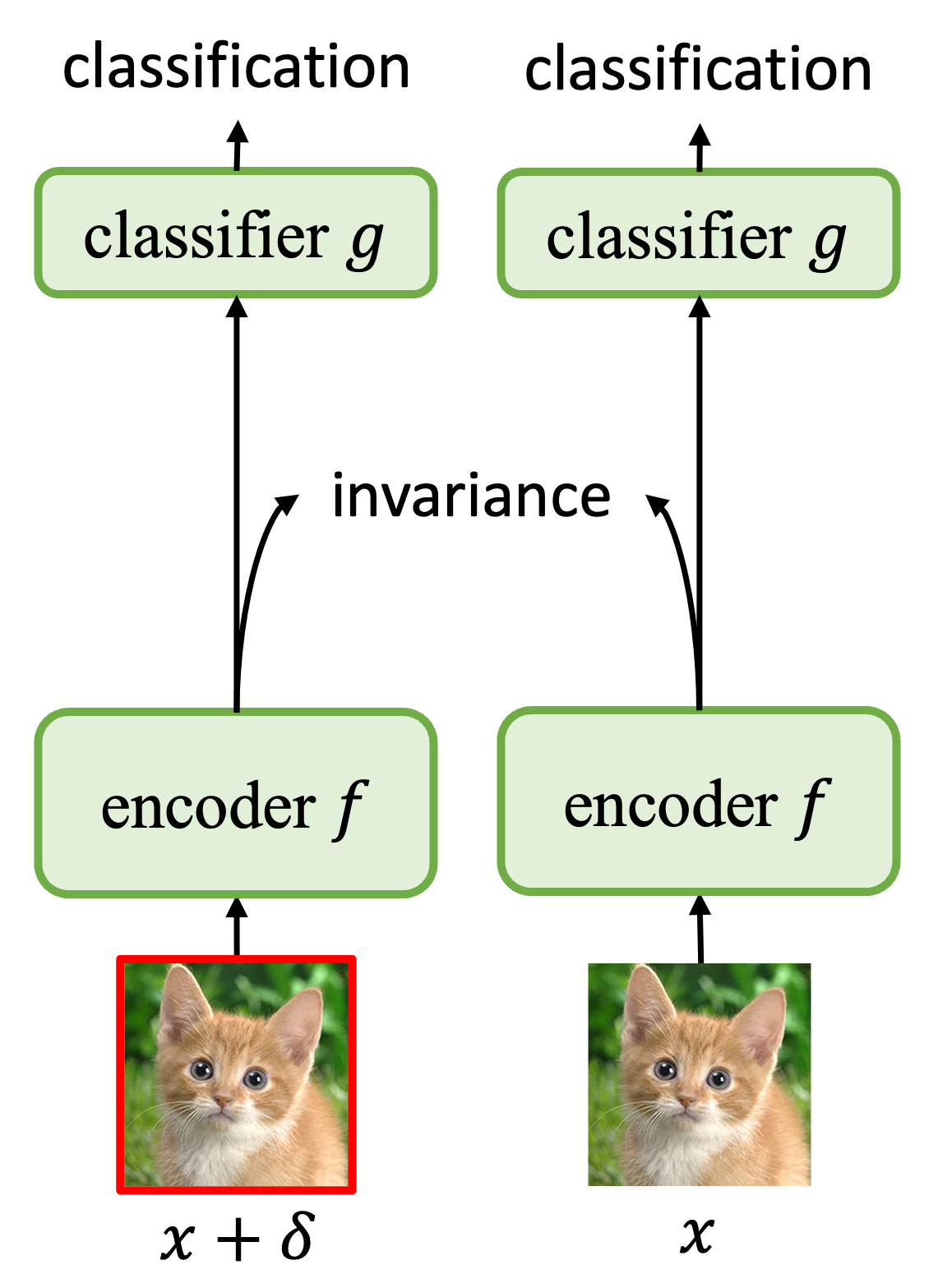
(a) Naive invariance regularization

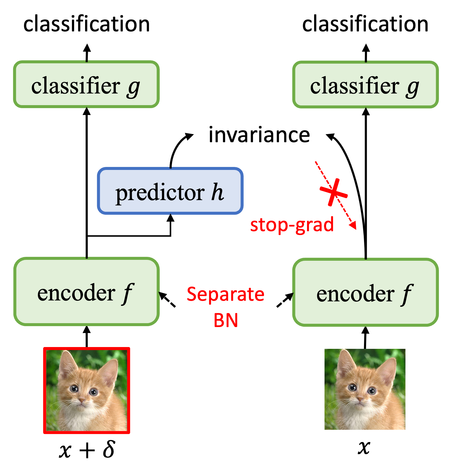
(b) Our approach: Asymmetrically Representation-regularized Adversarial Training (AR-AT)

Figure 1: Illustration of our approach. (a) Naive invariance regularization suffers from a “gradient conflict” between invariance loss and classification objectives, and a large distribution gap between clean and adversarial inputs. (b) Our approach uses an asymmetric structure with a stop-gradient operation and a predictor to avoid “gradient conflict”, and a split-BatchNorm (BN) to maintain consistent batch statistics during training.

Computer vision models based on deep neural networks (DNNs) achieve remarkable performance in various tasks. However, they are vulnerable to adversarial examples (AEs) (Szegedy et al., 2014; Goodfellow et al., 2015), which are carefully perturbed inputs to fool DNNs. Since AEs can fool DNNs without affecting human perception, they are a severe threat to real-world DNN applications.

Among the defense strategies against AEs, adversarial training (AT) (Goodfellow et al., 2015; Madry et al., 2018) has been the state-of-the-art approach, which augments the training data with AEs to enhance robustness. However, it is widely recognized that AT-based methods suffer from a trade-off between robustness and accuracy (Tsipras et al., 2019): to achieve high robustness, they sacrifice accuracy on clean images. Despite the extensive number of studies on AT-based methods, this robustness-accuracy trade-off has been a huge obstacle to their practical use.

To this end, we investigate the following research question: “How can a model learn adversarially invariant representation without losing discriminative power?.” Specifically, we focus on representation-based invariance regularization for AT-based methods, in contrast to most of the existing defenses (Zhang et al., 2019; Wang et al., 2019) that employ invariance regularization on the predicted outputs.

Our investigation reveals two key issues with naively applying invariance regularization (Fig.1(a)): (1) a “gradient conflict” between invariance loss and classification objectives, indicating the existence of “collapsing solutions,” and (2) the mixture distribution problem within Batch Normalization (BN) layers when the same BNs are used for both clean and adversarial inputs. “Gradient conflict” occurs when gradients for multiple loss functions oppose each other during joint optimization. Therefore, the observed conflict suggests that minimizing invariance loss may push the model toward non-discriminative directions. We hypothesize that it arises from the existence of “collapsing solutions” (Chen & He, 2021), i.e., a trivial solution for achieving invariance by encoding constant outputs. Furthermore, we find that using the same BNs for both clean and adversarial inputs causes the mixture distribution problem: the BNs are updated to have a mixture distribution of clean and adversarial inputs, which can be suboptimal for both clean and adversarial inputs.

To address these issues, we propose a novel method called Asymmetrically Representation-regularized Adversarial Training (AR-AT), incorporating a stop-gradient operation and a predictor, inspired by a modern non-contrastive self-supervised learning approach (Chen & He, 2021), and a split-BN structure, as depicted in Fig. 1(b). By employing the stop-gradient operation and predictor, AR-AT effectively avoids “collapsing solutions” and mitigates the “gradient conflict” between invariance loss and classification objectives during training. Additionally, the split-BN structure plays a key role in achieving high robustness and accuracy by resolving the mixture distribution problem. With both components combined, our method learns adversarially invariant representations without sacrificing discriminative power, leading to high robustness and accuracy.

Furthermore, we discuss the relevance of our findings to existing knowledge distillation (KD)-based defenses (Cui et al., 2021; Suzuki et al., 2023), which their relative successes had not been well understood. Specifically, we attribute their relative success to avoiding “collapsing solutions” by allowing variance between the teacher and student models and resolving the mixture distribution problem by using separate networks for clean and adversarial inputs.

Our contributions are summarized as follows:

• We rethink the representation-based invariance regularization in adversarial training to achieve high robustness without sacrificing accuracy.

• We reveal two key issues hindering invariance regularization: (1) a “gradient conflict” between invariance loss and classification objectives, and (2) the mixture distribution problem within Batch Norm (BN) layers.

• We propose a novel method AR-AT to incorporate a stop-gradient operation and a predictor, inspired by a recent non-contrastive self-supervised learning approach, and a split-BN structure.

• Our method significantly improves the robustness-accuracy trade-off by effectively learning discriminative yet adversarially invariant representations.

• We provide a new perspective on the relative success of knowledge distillation-based defenses, attributing it to avoiding “collapsing solutions” and resolving the mixture distribution problem.

2 Preliminaries

2.1 Adversarial Attack

Let $x\in\mathbb{R}^{d}$ be an input image and $y\in\{1,\dots,K\}$ be a class label from a data distribution $\mathcal{D}$. Let $f_{\theta}:\mathbb{R}^{d}\rightarrow\mathbb{R}^{K}$ be a DNN model parameterized by $\theta$. Adversarial attacks aim to find a perturbation $\delta$ that fools the model $f_{\theta}$ by solving the following optimization problem:

$$x^{\prime}=\mathop{\rm arg~{}max}\limits_{\delta\in\mathcal{S}}\mathcal{L}(f_{\theta}(x+\delta),y)$$ (1)

where $x^{\prime}$ is an adversarial example, $\mathcal{S}$ is a set of allowed perturbations, and $\mathcal{L}$ is a loss function. In this paper, we define the set of allowed perturbations $\mathcal{S}$ with $L_{\infty}$-norm as $\mathcal{S}=\{\delta\in\mathbb{R}^{d}\mid\|\delta\|_{\infty}\leq\epsilon\}$, where $\epsilon$ represents the size of the perturbations. The optimization of Eq.1 is often solved iteratively based on the projected gradient descent (PGD) (Madry et al., 2018).

2.2 Adversarial Training

Adversarial training (AT) (Goodfellow et al., 2015; Madry et al., 2018), which augments the training data with adversarial examples (AEs), has been the state-of-the-art approach to defend against adversarial attacks. Originally, Goodfellow et al. (2015) proposed to train the model with AEs generated by the fast gradient sign method (FGSM); in contrast, Madry et al. (2018) proposed to train a model with much stronger AEs generated by PGD, which is an iterative version of FGSM. Formally, the standard AT (Madry et al., 2018) solves the following optimization problem:

$$\min_{\theta}\mathop{\mathbb{E}}_{(x,y)\sim\mathcal{D}}\left[\max_{\delta\in\mathcal{S}}\mathcal{L}(f_{\theta}(x+\delta),y)\right]$$ (2)

where the inner maximization problem is solved iteratively based on PGD.

2.3 Invariance Regularization-based Defense

Table 1: Comparison of loss functions of defense methods. $f_{\theta}(\cdot)$ is the predictions of the trained model, and $z_{(\theta)}$ and $z^{\prime}_{(\theta)}$ is the latent representation of the model $f_{\theta}$ on clean and adversarial inputs, respectively. LBGAT and ARREST are knowledge distillation-based methods using a teacher model $g_{\phi}$. Our method AR-AT uses both clean and adversarial classification losses and employs representation-based regularization (Details in Sec. 3).

Method	Classification Loss		Regularization Loss
	Adversarial	Clean
AT	$CE(f_{\theta}(x^{\prime}),y)$
TRADES		$CE(f_{\theta}(x),y)$	$KL(f_{\theta}(x)||f_{\theta}(x^{\prime}))$
MART	$BCE(f_{\theta}(x^{\prime}),y)$		$KL(f_{\theta}(x)||f_{\theta}(x^{\prime}))\cdot(1-f_{\theta}(x)_{y})$
LBGAT		$CE(g_{\phi}(x),y)$	$MSE(f_{\theta}(x^{\prime}),g_{\phi}(x))$
ARREST	$CE(f_{\theta}(x^{\prime}),y)$		$CosSim(z^{\prime}_{(\theta)},z_{(\phi)})$, where $g_{\phi}$ is a fixed std. model
AR-AT (ours)	$CE(f_{\theta}(x^{\prime}),y)$	$CE(f_{\theta}^{\text{auxBN}}(x),y)$	$CosSim(h(z^{\prime}_{(\theta)}),\text{stop-grad}(z_{(\theta^{\text{auxBN}})}))$

While AT only inputs AEs during training, invariance regularization-based adversarial defense methods (Zhang et al., 2019; Wang et al., 2019) input both clean and adversarial images to ensure adversarial invariance of the model. TRADES (Zhang et al., 2019) introduces a regularization term on the logits to encourage adversarially invariant predictions; although it allows trade-off adjustment by altering the regularization strength, it still suffers from a trade-off. MART (Wang et al., 2019) further improved TRADES by focusing more on the misclassified examples to enhance robustness, still sacrificing clean accuracy. Unlike these logit-based invariance regularization methods, we explore representation invariance to mitigate the trade-off.

Another line of research is to employ knowledge distillation (KD) (Hinton et al., 2014)-based regularization, which has been shown effective in mitigating the trade-off. Cui et al. (2021) proposed LBGAT, which aligns the student model’s predictions on adversarial images with the standard model’s predictions on clean images, encouraging similarity of predictions between a student and a standardly trained teacher network. More recently, Suzuki et al. (2023) proposed ARREST, which performs representation-based KD so that the student model’s representations are similar to the standardly trained model’s representations. In contrast to these KD-based methods, which enforce adversarial invariance implicitly, we investigate output invariance within a single model, potentially more effective and more memory-efficient during training. Furthermore, we provide a new perspective on the relative success of KD-based methods, which had not been well understood.

Tab. 1 summarizes the loss functions of these methods and compares them with our method.

3 Method: Asymmetrically Representation-regularized Adversarial Training (AR-AT)

In this section, we propose a novel approach to effectively learn adversarially invariant representation without sacrificing discriminative power on clean images.

A straightforward approach to learn adversarially invariant representation is to employ a siamese structured invariance regularization, depicted in Fig. 1(a), as follows:

$$\mathcal{L}_{V0}=\alpha\cdot\mathcal{L}(f_{\theta}(x^{\prime}),y)+\beta\cdot\mathcal{L}(f_{\theta}(x),y)+\gamma\cdot Dist(z,z^{\prime})$$ (3)

where $x^{\prime}$ is an AE generated from $x$, $z$ and $z^{\prime}$ are the latent representations of $x$ and $x^{\prime}$, respectively. $\mathcal{L}$ is a classification loss and $Dist$ is a distance metric.

However, we identify two key issues hindering this naive approach: (1) a “gradient conflict” between invariance loss and classification objectives, and (2) the mixture distribution problem arising from diverged distributions of clean and adversarial inputs.

To address these issues, we propose a novel approach incorporating (1) a stop-gradient operation and a predictor MLP, inspired by modern non-contrastive self-supervised learning (Chen & He, 2021), and (2) a split-BatchNorm (BN) structure.

3.1 Stop-Gradient Operation and Predictor

Although naive invariance regularization (Eq.3) is a straightforward approach for learning adversarially invariant representation, we observed a “gradient conflict” between invariance loss and classification objectives, as shown in Fig. 2. “Gradient conflict” occurs when gradients for multiple loss functions oppose each other during joint optimization. Resolving “gradient conflict” has been shown to enhance performance in various fields, including multi-task learning (Yu et al., 2020) and domain generalization tasks with multiple domains (Mansilla et al., 2021). In this work, we point out that resolving “gradient conflict” is also crucial in learning discriminative yet adversarially invariant representation.

To resolve “gradient conflict”, we propose employing two components in the invariance regularization: (i) a stop-gradient operation and (ii) a predictor MLP, inspired by recent advancements in non-contrastive self-supervised learning (Grill et al., 2020; Chen & He, 2021), as illustrated in Fig. 1(b). These components are known to be effective in avoiding “collapsing solutions,” trivial solutions of encoding constant outputs to achieve invariance (Chen & He, 2021). The importance of these components to make the regularization term asymmetric has also been theoretically supported by recent efforts (Zhang et al., 2022; Wen & Li, 2022; Zhuo et al., 2023). In this work, we employ these components based on our hypothesis that the observed “gradient conflict” emerges from the difficulty in learning both adversarially invariant and discriminative representations simultaneously: minimizing invariance loss may push the model towards non-discriminative directions, as achieving invariance can easily be achieved by learning non-discriminative representations, such as constant outputs (i.e., “collapsing solutions”). Specifically, we employ (i) a stop-gradient operation on $z$ and (ii) a predictor MLP $h$ to the latent representations $z^{\prime}$ to predict $z$, and the Eq. 3 is modified as follows:

$$\mathcal{L}_{V1}=\alpha\cdot\mathcal{L}(f_{\theta}(x^{\prime}),y)+\beta\cdot\mathcal{L}(f_{\theta}(x),y)$$

$$+\;\gamma\cdot Dist(h(z^{\prime}),\text{stop-grad}(z))$$ (4)

where $\text{stop-grad}(\cdot)$ stops the gradient backpropagation from $z$ to $z^{\prime}$, treating $z$ as a constant, and $h$ is a predictor MLP. Here, the invariance regularization is unidirectional: we aim to bring the potentially corrupted adversarial representation $z^{\prime}$ closer to the clean representation $z$ by treating $z$ as a constant, but not vice versa.

In Sec. 5.1, we demonstrate that employing the stop-gradient operation and predictor resolves the “gradient conflict” between invariance loss and classification objectives by effectively avoiding “collapsing solutions.”

3.2 Split Batch Normalization

In addition to the problem of “gradient conflict”, we point out that using the same Batch Norm (BN) layers for both clean and adversarial inputs can lead to difficulty in achieving high performance due to a “mixture distribution problem.” Batch Norm (BN) (Ioffe & Szegedy, 2015) is a widely used technique to accelerate the training of DNNs, which normalizes the activations of the previous layer and then scales/shifts them by a learnable linear layer. However, since clean and adversarial inputs have diverged distributions, using the same BNs on a mixture of clean and adversarial inputs can be suboptimal for both clean and adversarial inputs, leading to reduced performance.

To address this issue, we employ a split-BN structure, which uses separate BNs for clean and adversarial inputs during training, inspired by Xie et al. (2019; 2020). Specifically, Eq. 4 is rewritten as follows:

$$\mathcal{L}_{V2}=\alpha\cdot\mathcal{L}(f_{\theta}(x^{\prime}),y)+\beta\cdot\mathcal{L}(f_{\theta}^{\text{auxBN}}(x),y)$$

$$+\;\gamma\cdot Dist(h(z^{\prime}_{(\theta)}),\text{stop-grad}(z_{(\theta^{\text{auxBN}})}))$$ (5)

where $f_{\theta}^{\text{auxBN}}$ shares parameters with $f_{\theta}$ but employs auxiliary BNs specialized for clean images, $z_{(\theta^{\text{auxBN}})}$ and $z^{\prime}_{(\theta)}$ are the latent representations of $x$ and $x^{\prime}$ from $f_{\theta}^{\text{auxBN}}$ and $f_{\theta}$, respectively. In this way, the BNs in $f_{\theta}$ exclusively processes adversarial inputs, while the BNs in $f_{\theta}^{\text{auxBN}}$ exclusively processes clean inputs, avoiding the mixture distribution problem.

Importantly, the split-BN structure is exclusively applied during training: During inference, the model $f_{\theta}$ is equipped to classify both clean and adversarial inputs with the same BNs. Therefore, in contrast to MBN-AT (Xie & Yuille, 2019) and AdvProp (Xie et al., 2020) that require test-time oracle selection of clean and adversarial BNs for optimal robustness and accuracy, our approach is more practical.

3.3 Reducing Hyperparameters with Auto-Balance

Furthermore, we employ a dynamic adjustment rule for the hyperparameters $\alpha$ and $\beta$, which control the balance between adversarial and clean classification loss. Specifically, we adjust $\alpha$ and $\beta$ based on the training accuracy of the previous epoch, inspired by Xu et al. (2023):

$$\alpha_{(t)} = Acc_{(t-1)}=\frac{1}{N}\sum_{i=1}^{N}\mathbb{I}(\text{argmax}(f^{\text{auxBN}}_{\theta_{t-1}}(x))=y)$$

$$\beta_{(t)} = 1-Acc_{(t-1)}$$ (6)

where $\alpha_{(t)}$ and $\beta_{(t)}$ are the hyperparameters at the current epoch $t$, and $Acc_{(t-1)}$ is the clean accuracy of the model $f_{\theta}^{\text{auxBN}}$ at the previous epoch $(t-1)$. This adjustment automatically forces the model to focus more on adversarial images as its accuracy on clean images improves. We empirically demonstrate that this heuristic dynamic adjustment strategy works well in practice, successfully reducing the hyperparameter tuning cost. We provide an ablation study in Sec. 7.1

3.4 Regularizing Multiple Level of Representations

Finally, our method is extended to regularize multiple levels of representations. Specifically, we employ multiple predictor MLPs $h_{1},\dots,h_{L}$ to enforce invariance across multiple levels of representations $z_{1},\dots,z_{L}$ as follows:

$$\frac{1}{L}\sum_{l=1}^{L}Dist(h_{l}(z^{\prime}_{(\theta),l}),\text{stop-grad}(z_{(\theta^{\text{auxBN}}),l}))$$ (7)

We found that regularizing multiple layers in the later stage of a network is the most effective, as demonstrated in our ablation study in Sec. 7.2.

4 Experimental Setup

Models and Datasets. We evaluate our method on CIFAR-10, CIFAR-100 (Krizhevsky & Hinton, 2009), and Imagenette (Howard, 2019) datasets. We use the standard data augmentation techniques of random cropping with 4 pixels of padding and random horizontal flipping. We use the model architectures of ResNet-18 (He et al., 2016) and WideResNet-34-10 (WRN-34-10) (Zagoruyko & Komodakis, 2016), following the previous works (Madry et al., 2018; Zhang et al., 2019; Cui et al., 2021).

Evaluation. We use 20-step PGD attack (PGD-20) (Madry et al., 2018) and AutoAttack (AA) (Croce & Hein, 2020) for evaluation. The perturbation budget is set to $\epsilon=8/255$. The step size is set to $2/255$ for PGD-20. We compare our method with the standard AT (Madry et al., 2018), and existing regularization-based methods TRADES (Zhang et al., 2019), MART (Wang et al., 2019), LBGAT (Cui et al., 2021), and ARREST (Suzuki et al., 2023).

Training Details. We use a 10-step PGD attack with cross-entropy loss for adversarial training. We initialized the learning rate to 0.1, divided it by a factor of 10 at the 75th and 90th epochs, and trained for 100 epochs. We use the SGD optimizer with a momentum of 0.9 and a weight decay of 5e-4, with a batch size of 128. We used Cosine Distance as the distance metric for invariance regularization. The predictor MLP has two linear layers, with the hidden dimension set to 1/4 of the feature dimension, following SimSiam (Chen & He, 2021). The latent representations to be regularized are spatially average-pooled to obtain one-dimensional vectors. The regularization strength $\gamma$ is set to 30.0 for ResNet-18 and 100.0 for WRN-34-10. We regularize all ReLU outputs in “layer4” for ResNet-18, and “layer3” for WRN-34-10.

5 Empirical Study

5.1 AR-AT Resolves “Gradient Conflict” and Mixture Distribution Problem

The stop-gradient operation and predictor MLP resolves “gradient conflict.” In Fig. 2, we plot the cosine similarity between the gradients of the classification loss (the sum of clean and adversarial classification loss) and the invariance loss with respect to $\theta$ during training. We observe that with the naive invariance regularization ($\mathcal{L}_{V0}$; Eq. 3), the gradient similarity fluctuates around zero, indicating that some neurons encounter “gradient conflict” during training. This indicates that minimizing invariance loss may push the model towards non-discriminative directions, as achieving invariance can easily be achieved by learning non-discriminative representations, such as constant outputs (i.e., “collapsing solutions”). In contrast, with the stop-gradient operation and predictor ($\mathcal{L}_{V1}$; Eq. 4), the gradient similarity becomes consistently positive. This demonstrates the effectiveness of avoiding “collapsing solutions” to resolve the “gradient conflict” when learning adversarially invariant representation, leveraging insights from modern non-contrastive self-supervised learning (Chen & He, 2021).

Nevertheless, Tab. 2 shows that mitigating “gradient conflict” ($\mathcal{L}_{V0}$ vs. $\mathcal{L}_{V1}$) only slightly improves the robustness and accuracy. We attribute this to another issue of the mixture distribution problem discussed next.

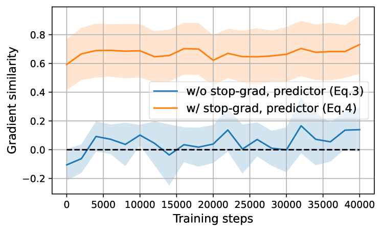
Figure 2: Gradient similarity between classification loss and invariance loss with respect to $\theta$ during training, with and without the stop-gradient operation and predictor. The light areas show the standard deviation of cosine similarity per layer, while the dark line represents the mean.

Table 2: Contributions of each component in AR-AT, for ResNet-18 trained on CIFAR10. “Grad-sim.” represents the average gradient similarity between the classification loss and invariance loss with respect to $\theta$ during training.

	Method
	Stop-grad + Pred. $h$	Split BN	Clean	PGD- 20	Grad- sim.
$\mathcal{L}_{V0}$			82.93	48.89	0.06
$\mathcal{L}_{V1}$	$\checkmark$		83.00	49.14	0.63
		$\checkmark$	84.35	51.34	0.14
$\mathcal{L}_{V2}$	$\checkmark$	$\checkmark$	86.29	52.40	0.52

Split-BN resolves the mixture distribution problem. Furthermore, we identify and tackle another challenge in learning adversarially invariant representations: using the same Batch Norm (BN) layers for both clean and adversarial inputs can hinder achieving high robustness and accuracy. Tab. 2 shows the comparison of invariance regularization with and without split-BN ($\mathcal{L}_{V1}$; Eq. 4 and $\mathcal{L}_{V2}$; Eq. 5, respectively), both of which employ the stop-gradient operation and predictor. We observe that using separate BNs for clean and adversarial inputs ($\mathcal{L}_{V2}$) significantly improves the robustness and accuracy compared to using the same BNs for both clean and adversarial inputs ($\mathcal{L}_{V1}$).

Importantly, Tab. 2 shows that only resolving either “gradient conflict” or mixture distribution problem does not significantly improve robustness and accuracy. Our results suggest that resolving both the “gradient conflict” and the mixture distribution problem is crucial to achieving high robustness and accuracy.

5.2 Comparison with State-of-the-Art Methods

Table 3: Comparison with state-of-the-art defense methods on CIFAR10 and CIFAR100. We report clean and robust accuracy against AutoAttack (AA). “Extra Param.” represents the additional parameters needed during training (e.g., knowledge distillation-based methods require a teacher network. LBGAT uses ResNet-18 as the teacher network). Results with ^∗ are directly copied from original papers.

	Defense		CIFAR10			CIFAR100
		Extra Param.	Clean	AA	Sum.	Clean	AA	Sum.
ResNet-18	AT		83.77	42.42	126.19	55.82	19.50	75.32
	TRADES		81.25	48.54	129.79	54.74	23.60	78.34
	MART		82.15	47.83	129.98	54.54	26.04	80.58
	LBGAT	+ 100.0%	85.50	49.26	134.76	67.33	23.94	91.21
	ARREST∗	+ 100.0%	86.63	46.14	132.77	-	-	-
	AR-AT (ours)	+ 0.9%	87.93	49.19	137.12	67.72	23.54	91.26
WRN-34-10	AT		86.06	46.26	132.32	59.83	23.94	83.77
	TRADES		84.33	51.75	136.08	57.61	26.88	84.49
	MART		86.10	49.11	135.21	57.75	24.89	82.64
	LBGAT	+ 25.0%	88.28	52.49	140.77	69.26	27.53	96.79
	ARREST∗	+ 100.0%	90.24	50.20	140.44	73.05	24.32	97.37
	AR-AT (ours)	+ 0.7%	90.81	51.19	142.00	72.23	24.97	97.20

Table 4: Comparison with state-of-the-art defense methods on Imagenette. We report clean accuracy and robust accuracy against AutoAttack (AA). (For LBGAT^†, we lowered the learning rate from default due to gradient explosion.)

	Defense	Imagenette
		Clean	AA	Sum.
ResNet-18	AT	84.58	52.25	136.83
	TRADES	79.21	53.98	133.19
	MART	84.07	59.89	143.96
	LBGAT†	80.80	50.42	131.22
	AR-AT (ours)	88.66	59.28	147.94

Tab. 3 shows the results of ResNet-18 and WRN-34-10 trained on CIFAR-10 and CIFAR-100. We observe that our method achieves much better performance than the baselines of regularization-based defenses TRADES and MART on both datasets, highlighting the effectiveness of our methodology in employing invariance regularization. Moreover, our method achieves state-of-the-art performance on CIFAR10 in mitigating the trade-off, outperforming LBGAT and ARREST, which employs implicit invariance regularization with knowledge distillation. On CIFAR-100, our method achieves comparable results to LBGAT and ARREST. Tab. 4 shows the results on Imagenette, a dataset with high-resolution images. We observe that our method achieves the best performance in terms of both robustness and accuracy. These results strongly support AR-AT’s effectiveness in mitigating the robustness-accuracy trade-off.

Furthermore, we highlight that training AR-AT is more memory-efficient than LBGAT and ARREST, which rely on a separate teacher network for knowledge distillation. This is crucial for large-scale model training, where memory usage can be a bottleneck.

5.3 AR-AT learns Adversarially Invariant yet Discriminative Representation

Table 5: Representation invariance analysis. “Cos. Sim.” represents cosine similarity between adversarial and clean features. “Sum.” denotes the sum of clean accuracy and robust accuracy against AutoAttack (AA).

	Defense	CIFAR10
		Sum.	Cos. Sim.
ResNet-18	AT	126.19	0.9423
	TRADES	129.79	0.9693
	MART	129.98	0.9390
	LBGAT	134.76	0.9236
	AR-AT (ours)	137.12	0.9450
WRN-34-10	AT	132.32	0.9290
	TRADES	136.08	0.9765
	MART	135.21	0.9040
	LBGAT	140.77	0.9015
	AR-AT (ours)	142.00	0.9483

Quantitative analysis. Tab. 5 presents representation invariance measured by cosine similarity between adversarial and clean features extracted from the penultimate layer. While TRADES achieves high adversarial invariance with logit-based regularization, it sacrifices accuracy; this demonstrates that adversarial invariance can be achieved by sacrificing discriminative power. Additionally, LBGAT, a KD-based method, achieves high performance but low adversarial invariance; this shows that using a separate teacher network for regularization does not ensure invariance within a model.

In contrast, AR-AT achieves both high adversarial invariance and high accuracy simultaneously. Therefore, the effectiveness of AR-AT is attributed to learning adversarially invariant yet discriminative representations by addressing the challenges of the “gradient conflict” and the mixture distribution problem in invariance regularization (Sec. 3).

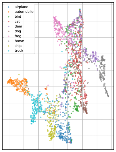
(a) Naive invariance regularization ($\mathcal{L}_{V0}$; Eq. 3)

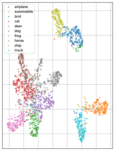
(b) AR-AT ($\mathcal{L}_{V2}$; Eq. 5), which incorporates stop-grad., predictor, and split-BN.

Figure 3: Visualization of clean representations for (a) naive invariance regularization ($\mathcal{L}_{V0}$, Eq. 3) and (b) AR-AT ($\mathcal{L}_{V2}$, Eq. 5) using UMAP (McInnes et al., 2018). 2000 clean images are randomly sampled from the CIFAR10 test set.

Visualization of learned representations. Fig. 3 visualizes the clean representations for (a) naive invariance regularization ($\mathcal{L}_{V0}$, Eq. 3) and (b) AR-AT ($\mathcal{L}_{V2}$, Eq. 5), using UMAP (McInnes et al., 2018). We observe that the naive invariance regularization ($\mathcal{L}_{V0}$) leads to relatively non-discriminative representations. This sacrifice of discriminative power is likely due to the model’s pursuit of adversarial invariance; In fact, the cosine similarity between adversarial and clean features was 0.9985, which is the highest among all methods in Tab. 5. In contrast, AR-AT (Fig. 3(b)) learns more discriminative representations compared to naive invariance regularization.

6 On the Relation of AR-AT to Knowledge Distillation (KD)

Despite the relative success of KD-based methods LBGAT and ARREST, the mechanism behind their effectiveness remains unclear. Here, we provide a new perspective on the success of KD-based methods. In this section, the hyperparameters $\alpha$ and $\beta$ are set to 1.0, and the penultimate layer is used for regularization loss for simplicity.

Using separate networks can be another solution to relieve the “gradient conflict” and the mixture distribution problem. Fig. 4 illustrates the impact of using “shared weights vs. separate networks” between adversarial and clean branches in AR-AT. We observe that “Naive Inv. Loss (Eq. 3)” and “AR-AT w/o Split-BN (Eq. 4)” failed to achieve high robustness when more weights are shared; in contrast, they achieve high robustness when using separate networks for clean and adversarial branches. This can be explained as follows: (1) Using separate networks acts similarly to the stop-gradient operation, preventing gradient flow between branches; (2) Separate networks avoid the mixture distribution problem. On the other hand, AR-AT (Eq. 5) maintains performance when layers are shared: Importantly, it even improves performance when layers are shared, indicating its superiority over KD-based regularization. This advantage of sharing layers stems from more explicit invariance regularization, in contrast to the implicit invariance regularization using a separate teacher network.

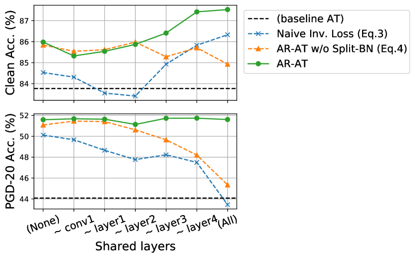
Figure 4: Comparison of “sharing parameters vs. separate networks” in AR-AT for adversarial and clean branches. The x-axis represents the depth until which parameters are shared: the leftmost corresponds to completely separate networks for two branches, while the rightmost shares all parameters (default).

Asymmetrizing logit-based regularization: Improving TRADES and its relation to LBGAT. Additionally, we explore the benefits of an asymmetric structure for logit-based regularization and its relation to KD. LBGAT outperforms TRADES (Tab. 3) by leveraging KD-based logit regularization with similar loss functions (Tab. 1). In Appendix D, we demonstrate that TRADES also face “gradient conflict” and the mixture distribution problem, and asymmetrizing TRADES via stop-gradient and split-BN structures leads to improved robustness and accuracy, resembling LBGAT. This reveals the overlooked issues in TRADES and suggests that LBGAT’s superiority is rooted in addressing two challenges of “gradient conflict” and the mixture distribution problem, providing deeper insights into the benefits of KD-based methods in adversarial robustness. Please refer to Appendix D for more details.

7 Ablation study

7.1 Effectiveness of Hyperparameter Auto-Balance

Tab. 6 shows an ablation study of AR-AT “with vs. without auto-balance (Sec. 3.3)” of the hyperparameters $\alpha$ and $\beta$, which controls the balance between adversarial and clean classification loss. The results demonstrate that auto-balancing performs comparable to the best hyperparameter manually obtained. Additionally, in the case of WRN-34-10, auto-balancing outperforms the best hyperparameter setting in Tab. 6, suggesting that it can discover superior hyperparameter configurations beyond manual tuning.

Table 6: Comparison of AR-AT “with vs. without auto-balance (Eq. 6)” of hyperparameter $\alpha$ and $\beta$ on CIFAR-10.

$(\alpha,\beta$)	ResNet-18		WRN-34-10
	Clean	PGD-20	Clean	PGD-20
$(1.0,1.0)$	88.91	51.75	91.39	49.17
$(1.0,0.5)$	88.55	52.12	91.48	49.01
$(1.0,0.1)$	87.55	52.27	90.80	49.46
$(0.5,1.0)$	89.01	51.37	91.71	50.35
$(0.1,1.0)$	89.08	46.73	91.85	48.51
auto-bal.	87.93	52.13	90.81	52.72

7.2 Layer Importance in Invariance Regularization

Tab. 7 shows the ablation study of AR-AT on regularizing different levels of latent representations. ResNet-18 and WRN-34-10 have four and three “layers”, respectively. “Layers” are composed of multiple “BasicBlocks”, which consist of multiple convolutional layers followed by BN and ReLU. We observed that instead of only regularizing the penultimate layer, regularizing multiple latent representations in the later stage of the network achieves higher robustness and accuracy. In practice, we recommend regularizing all ReLU outputs in the last stage of the network, which is the default setting in our experiments. Nevertheless, we note that the choice of layers for invariance regularization is not critical as long as the latent representations in the later stage of the network are regularized.

Table 7: Choice of regularized layers in AR-AT on CIFAR-10.

	Regularized Layers	Clean	PGD-20
ResNet	Penultimate layer (“layer4”)	86.28	51.78
	“layer3”, “layer4”	87.35	52.27
	All BasicBlocks in “layer4”	87.16	52.27
	All ReLUs in “layer4” (default)	87.93	52.13
WRN	Penultimate layer (“layer3”)	88.87	52.50
	“layer2”, “layer3”	88.95	50.74
	All BasicBlocks in “layer3”	89.50	51.76
	All ReLUs in “layer3” (default)	90.81	52.72

7.3 Importance of BatchNorm for Robustness

Tab. 8 reports the performance of AR-AT when the auxiliary BNs are used during inference. Intriguingly, although all the layers except BNs are shared between $f_{\theta}$ and $f_{\theta}^{\text{auxBN}}$, using the auxiliary BNs during inference notably enhances the clean accuracy while significantly compromising robustness, indicating that the auxiliary BNs are exclusively tailored for clean inputs. This shows the critical role of BNs, which constitute less than 0.1% of total parameters, in achieving high robustness.

Table 8: Importance of BatchNorm. We compare AR-AT using main BNs or auxiliary BNs during inference on CIFAR10.

	Defense	Clean	PGD-20
ResNet-18	AR-AT ($f_{\theta}$)	87.93	52.13
	AR-AT ($f_{\theta}^{\text{auxBN}}$)	92.84	1.98

8 Conclusion

In this paper, we introduce AR-AT to mitigate the robustness-accuracy trade-off. By addressing two challenges of the “gradient conflict” and the “mixture distribution problem,” AR-AT learns discriminative yet adversarially invariant representations. The “gradient conflict” between the classification loss and invariance loss arises from the existence of “collapsing solutions” of outputting adversarially invariant yet non-discriminative representations. This is resolved by employing a stop-gradient operation and a predictor MLP inspired by modern self-supervised learning. Meanwhile, the mixture distribution problem stems from a large distribution gap between adversarial and clean images. We mitigate this by employing a split-BN structure to process the adversarial and clean images with different BNs. By effectively learning discriminative yet adversarially invariant representations, AR-AT achieves the state-of-the-art performance of mitigating the trade-off. Furthermore, we provide a new perspective to the knowledge distillation-based defense methods, which has not been well understood: we attribute their relative success to resolving “gradient conflict” and the “mixture distribution problem.” This paper provides a novel perspective to mitigate the robustness-accuracy trade-off.

9 Impact Statement

This paper provides a new perspective and valuable insights toward realizing reliable and trustworthy machine learning. We do not see any negative societal consequences of our work.

Appendix A Datasets

Here, we provide the details of the datasets we used in our experiments. CIFAR10 and CIFAR100 (Krizhevsky & Hinton, 2009) are standard datasets for image classification with 10 and 100 classes, respectively, with a resolution of $32\times 32$. Imagenette (Howard, 2019) is a subset of 10 easily classified classes from Imagenet (Deng et al., 2009). In our experiments, we used the version with the resolution of $160\times 160$.

Table 9: The details of datasets we used in our experiments.

Dataset	Resolution	Class Num.	Train	Val
CIFAR10	32 $\times$ 32	10	50,000	10,000
CIFAR100	32 $\times$ 32	100	50,000	10,000
Imagenette	160 $\times$ 160	10	9,469	3,925

Appendix B Implementation Details of Baseline Methods

Here, we describe the implementation details of the baseline methods we compared in our experiments.

• Adversarial Training (AT) (Madry et al., 2018): We use the simple implementation by Dongbin Na . We aligned the hyperparameter setting described in the official GitHub repository .

• TRADES (Zhang et al., 2019): We use the official implementation  and used the default hyperparameter setting.

• MART (Wang et al., 2019): We use the official implementation  and used the default hyperparameter setting.

• LBGAT (Cui et al., 2021): We use the official implementation  and used the default hyperparameter setting. For Imagenette, we observed that the default learning rate causes gradient explosion, so we lowered the learning rate from 0.1 to 0.01. Note that LBGAT uses a ResNet-18 teacher network for both ResNet-18 and WRN-34-10 student networks.

• ARREST (Suzuki et al., 2023): They do not provide an official implementation, so we directly copied the results in Tab. 3 from their paper.

Appendix C More Comparison with State-of-the-Art Defense Methods

Table 10: Comparison of clean accuracy and robust accuracy against AutoAttack (AA) for WideResNet-34-10 trained on CIFAR10. The compared methods are sorted by the sum of clean and robust accuracy.

Method	Clean	AutoAttack	Sum.	Reference
AT (Madry et al., 2018)	86.06	46.26	132.32	Reproduced
FAT (Zhang et al., 2020)	89.34	43.05	132.39	Copied from (Suzuki et al., 2023)
MART (Wang et al., 2019)	86.10	49.11	135.21	Reproduced
TRADES (Zhang et al., 2019)	84.33	51.75	136.08	Reproduced
IAD (Zhu et al., 2021)	85.09	52.29	137.38	Copied from the original paper
AWP (Wu et al., 2020)	85.57	54.04	139.61	Copied from the original paper
S2O (Jin et al., 2022)	85.67	54.10	139.77	Copied from the original paper
ARREST (Suzuki et al., 2023)	90.24	50.20	140.44	Copied from the original paper
LBGAT (Cui et al., 2021)	88.28	52.49	140.77	Reproduced
AR-AT (ours)	90.81	51.19	142.00	(Ours)

Table 11: Comparison of clean accuracy and robust accuracy against AutoAttack (AA) for WideResNet-34-10 trained on CIFAR100. The compared methods are sorted by the sum of clean and robust accuracy.

Method	Clean	AutoAttack	Sum.	Reference
MART (Wang et al., 2019)	57.75	24.89	82.64	Reproduced
AT (Madry et al., 2018)	59.83	23.94	83.77	Reproduced
TRADES (Zhang et al., 2019)	57.61	26.88	84.49	Reproduced
FAT (Zhang et al., 2020)	65.51	21.17	86.68	Copied from (Suzuki et al., 2023)
IAD (Zhu et al., 2021)	60.72	27.89	88.61	Copied from the original paper
AWP (Wu et al., 2020)	60.38	28.86	89.24	Copied from the original paper
S2O (Jin et al., 2022)	63.40	27.60	91.00	Copied from the original paper
LBGAT (Cui et al., 2021)	69.26	27.53	96.79	Reproduced
ARREST (Suzuki et al., 2023)	73.05	24.32	97.37	Copied from the original paper
AR-AT (ours)	72.23	24.97	97.20	(Ours)

We provide more comparison with state-of-the-art defense methods in Tab. 10 and Tab. 11 We observe that AR-AT achieves high clean accuracy while maintaining high robustness. These results demonstrate the effectiveness of AR-AT in mitigating the robustness-accuracy trade-off.

Appendix D Asymmetrizing Logit-based Regularization: Improving TRADES and Its Relation to LBGAT

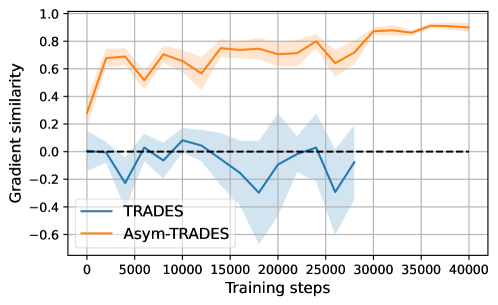
Figure 5: Comparison of gradient similarity between “TRADES vs. Asymmetrized-TRADES (Asym-TRADES)”. We compare gradient similarity between the classification loss and invariance loss with respect to $\theta$ during training.

The main text mainly focused on employing representation-based invariance regularization to mitigate the robustness-accuracy trade-off. Thus, this section discusses logit-based invariance regularization, such as TRADES (Zhang et al., 2019) and LBGAT (Cui et al., 2021), and shows that similar discussion to representation-based regularization methods is applicable for logit-based regularization.

TRADES also suffers from “gradient conflict.” In Fig. 5, we visualize the gradient similarity between the classification loss and invariance loss with respect to $\theta$ during training. TRADES also suffers from “gradient conflict,” where the gradient similarity between the classification loss is negative for many layers. This can be explained by the difficulty in achieving prediction invariance while maintaining discriminative power, which is the same reason why the naive invariance regularization (Eq. 3) suffers from “gradient conflict” (Sec. 3.1).

Table 12: Comparison of loss functions between TRADES, Asymmetrized-TRADES, and LBGAT. LBGAT is similar to TRADES, except that it employs a separate teacher network to regularize the student network.

Method	Classification Loss		Regularization Loss
	Adversarial	Clean
TRADES		$CE(f_{\theta}(x),y)$	$KL(f_{\theta}(x)||f_{\theta}(x^{\prime}))$
Asym-TRADES	$CE(f_{\theta}(x^{\prime}),y)$	$CE(f_{\theta}^{\text{auxBN}}(x),y)$	$KL(f_{\theta}(x^{\prime})||\text{stop-grad}(f_{\theta}^{\text{auxBN}}(x)))$
LBGAT		$CE(g_{\phi}(x),y)$	$MSE(f_{\theta}(x^{\prime}),g_{\phi}(x))$

Table 13: Comparison of TRADES vs. Asym-TRADES for ResNet18 trained on CIFAR10.

Method	Clean	AutoAttack
TRADES	81.25	48.54
Asym-TRADES	85.62	48.58
w/o Stop-grad	82.13	48.97
w/o Split-BN	80.90	49.93
LBGAT	85.50	49.26

Aymmetrizing TRADES with stop-gradient operation and split-BN. To further validate our findings, we consider asymmetrizing TRADES based on AR-AT’s strategy. Specifically, we replace the regularization term of AR-AT with TRADES’s regularization term, which we call “Asym-TRADES,” as shown in Tab. 12. Here, we did not employ the predictor MLP in Asym-TRADES since having a bottleneck-structured predictor MLP does not make sense for logits. Similar to the phenomenon in representation-based regularization, Asym-TRADES does not suffer from “gradient conflict” (Fig. 5), and achieves higher robustness and accuracy than TRADES (Tab. 13).

Asymmetrized TRADES achieve approximately the same performance as LBGAT. Intriguingly, Tab. 13 demonstrates that Asym-TRADES achieve approximately the same performance as LBGAT. This validates our hypothesis that the effectiveness of the KD-based method LBGAT can be attributed to resolving “gradient conflict” and the mixture distribution problem, as discussed in Sec. 6. LBGAT employs a separate teacher network to regularize the student network, which implicitly resolves the “gradient conflict” and the mixture distribution problem.

Appendix E Additional Ablation Study

E.1 Contributions of Each Component in AR-AT

Tab. 14 shows the abltation study of three components in AR-AT: stop-gradient operation, predictor MLP, and split-BN. The results demonstrate that Split-BN consistently improves the robustness and accuracy compared to the naive invariance regularization (i.e., (1) in Tab. 14) by mitigating the mixture distribution problem. On the other hand, we observe that mitigation of “gradient conflict” does not necessarily improve the robustness and accuracy (i.e., (2) and (4) in Tab. 14): it is explicitly effective when the mixture distribution problem is resolved by split-BN (i.e., (8) in Tab. 14). Therefore, we conclude that resolving both issues of “gradient conflict” and mixture distribution problem is important to achieve high robustness and accuracy.

Table 14: Contributions of each component in AR-AT, for ResNet-18 trained on CIFAR10. “Grad-sim.” represents the average gradient similarity between the classification loss and invariance loss with respect to $\theta$ during training. Here, the penultimate representation is regularized.

	Method
	Stop-grad	Pred.	Split-BN	Clean	PGD-20	Grad-sim.
(1) $\mathcal{L}_{V0}$				82.93	48.89	0.06
(2)	$\checkmark$			82.47	48.57	0.68
(3)		$\checkmark$		83.49	48.22	0.00
(4) $\mathcal{L}_{V1}$	$\checkmark$	$\checkmark$		83.00	49.14	0.63
(5)			$\checkmark$	84.35	51.34	0.14
(6)	$\checkmark$		$\checkmark$	85.51	51.46	0.59
(7)		$\checkmark$	$\checkmark$	84.07	50.79	0.00
(8) $\mathcal{L}_{V2}$	$\checkmark$	$\checkmark$	$\checkmark$	86.29	52.40	0.52

E.2 Strength of Invariance Regularization $\gamma$

Tab. 15 shows the ablation study of AR-AT on the strength of invariance regularization $\gamma$. We observe that the performance is not too sensitive to the strength of invariance regularization $\gamma$. Nevertheless, the optimal $\gamma$ depends on the architecture. For example, $\gamma=30.0$ is optimal for ResNet-18, while $\gamma=100.0$ is optimal for WRN-34-10.

Table 15: AR-AT’s sensitivity to the strength of invariance regularization $\gamma$.

		CIFAR10		CIFAR100
	$\gamma$	Clean	PGD-20	Clean	PGD-20
ResNet-18	10.0	87.90	51.53	66.89	26.79
	30.0 (default)	87.93	52.13	68.07	26.76
	50.0	87.54	51.27	67.72	26.52
	100.0	87.06	50.14	66.19	26.02
	120.0	86.46	50.15	65.31	25.71
WRN-34-10	10.0	89.21	48.71	67.46	26.86
	30.0	90.93	49.68	70.69	26.86
	50.0	91.36	50.51	71.52	26.46
	100.0 (default)	91.29	52.24	71.58	28.06
	120.0	91.39	51.94	71.92	27.31

References

- Chen & He (2021) Chen, X. and He, K. Exploring simple siamese representation learning. In Proceedings of the IEEE/CVF conference on computer vision and pattern recognition, pp. 15750–15758, 2021.
- Croce & Hein (2020) Croce, F. and Hein, M. Reliable evaluation of adversarial robustness with an ensemble of diverse parameter-free attacks. In International conference on machine learning, pp. 2206–2216. PMLR, 2020.
- Cui et al. (2021) Cui, J., Liu, S., Wang, L., and Jia, J. Learnable boundary guided adversarial training. In Proceedings of the IEEE/CVF international conference on computer vision, pp. 15721–15730, 2021.
- Deng et al. (2009) Deng, J., Dong, W., Socher, R., Li, L.-J., Li, K., and Fei-Fei, L. Imagenet: A large-scale hierarchical image database. In 2009 IEEE conference on computer vision and pattern recognition, pp. 248–255. Ieee, 2009.
- Goodfellow et al. (2015) Goodfellow, I. J., Shlens, J., and Szegedy, C. Explaining and harnessing adversarial examples. In ICLR, 2015.
- Grill et al. (2020) Grill, J.-B., Strub, F., Altché, F., Tallec, C., Richemond, P., Buchatskaya, E., Doersch, C., Avila Pires, B., Guo, Z., Gheshlaghi Azar, M., et al. Bootstrap your own latent-a new approach to self-supervised learning. Advances in neural information processing systems, 33:21271–21284, 2020.
- He et al. (2016) He, K., Zhang, X., Ren, S., and Sun, J. Deep residual learning for image recognition. In Proceedings of the IEEE/CVF Confer- ence on Computer Vision and Pattern Recognition, pp. 770–778, 2016.
- Hinton et al. (2014) Hinton, G., Vinyals, O., and Dean, J. Distilling the knowledge in a neural network. Workshop on Advances in neural information processing systems, 2014.
- Howard (2019) Howard, J. A smaller subset of 10 easily classified classes from imagenet, and a little more french. https://github.com/fastai/imagenette, 2019.
- Ioffe & Szegedy (2015) Ioffe, S. and Szegedy, C. Batch normalization: Accelerating deep network training by reducing internal covariate shift. In International conference on machine learning, pp. 448–456. pmlr, 2015.
- Jin et al. (2022) Jin, G., Yi, X., Huang, W., Schewe, S., and Huang, X. Enhancing adversarial training with second-order statistics of weights. In Proceedings of the IEEE/CVF Conference on Computer Vision and Pattern Recognition, pp. 15273–15283, 2022.
- Krizhevsky & Hinton (2009) Krizhevsky, A. and Hinton, G. Learning multiple layers of features from tiny images. Technical report, University of Toronto, 2009.
- Madry et al. (2018) Madry, A., Makelov, A., Schmidt, L., Tsipras, D., and Vladu, A. Towards deep learning models resistant to adversarial attacks. In ICLR, 2018.
- Mansilla et al. (2021) Mansilla, L., Echeveste, R., Milone, D. H., and Ferrante, E. Domain generalization via gradient surgery. In Proceedings of the IEEE/CVF international conference on computer vision, pp. 6630–6638, 2021.
- McInnes et al. (2018) McInnes, L., Healy, J., and Melville, J. Umap: Uniform manifold approximation and projection for dimension reduction. arXiv preprint arXiv:1802.03426, 2018.
- Suzuki et al. (2023) Suzuki, S., Yamaguchi, S., Takeda, S., Kanai, S., Makishima, N., Ando, A., and Masumura, R. Adversarial finetuning with latent representation constraint to mitigate accuracy-robustness tradeoff. In 2023 IEEE/CVF International Conference on Computer Vision (ICCV), pp. 4367–4378. IEEE, 2023.
- Szegedy et al. (2014) Szegedy, C., Zaremba, W., Sutskever, I., Bruna, J., Erhan, D., Goodfellow, I., and Fergus, R. Intriguing properties of neural networks. In ICLR, 2014.
- Tsipras et al. (2019) Tsipras, D., Santurkar, S., Engstrom, L., Turner, A., and Madry, A. Robustness may be at odds with accuracy. In ICLR, 2019.
- Wang et al. (2019) Wang, Y., Zou, D., Yi, J., Bailey, J., Ma, X., and Gu, Q. Improving adversarial robustness requires revisiting misclassified examples. In International conference on learning representations, 2019.
- Wen & Li (2022) Wen, Z. and Li, Y. The mechanism of prediction head in non-contrastive self-supervised learning. Advances in Neural Information Processing Systems, 35:24794–24809, 2022.
- Wu et al. (2020) Wu, D., Xia, S.-T., and Wang, Y. Adversarial weight perturbation helps robust generalization. Advances in Neural Information Processing Systems, 33:2958–2969, 2020.
- Xie & Yuille (2019) Xie, C. and Yuille, A. Intriguing properties of adversarial training at scale. arXiv preprint arXiv:1906.03787, 2019.
- Xie et al. (2020) Xie, C., Tan, M., Gong, B., Wang, J., Yuille, A. L., and Le, Q. V. Adversarial examples improve image recognition. In Proceedings of the IEEE/CVF conference on computer vision and pattern recognition, pp. 819–828, 2020.
- Xu et al. (2023) Xu, X., Zhang, J., and Kankanhalli, M. Autolora: A parameter-free automated robust fine-tuning framework. arXiv preprint arXiv:2310.01818, 2023.
- Yu et al. (2020) Yu, T., Kumar, S., Gupta, A., Levine, S., Hausman, K., and Finn, C. Gradient surgery for multi-task learning. Advances in Neural Information Processing Systems, 33:5824–5836, 2020.
- Zagoruyko & Komodakis (2016) Zagoruyko, S. and Komodakis, N. Wide residual networks. arXiv preprint arXiv:1605.07146, 2016.
- Zhang et al. (2022) Zhang, C., Zhang, K., Zhang, C., Pham, T. X., Yoo, C. D., and Kweon, I. S. How does simsiam avoid collapse without negative samples? a unified understanding with self-supervised contrastive learning. International conference on learning representations, 2022.
- Zhang et al. (2019) Zhang, H., Yu, Y., Jiao, J., Xing, E., El Ghaoui, L., and Jordan, M. Theoretically principled trade-off between robustness and accuracy. In International conference on machine learning, pp. 7472–7482. PMLR, 2019.
- Zhang et al. (2020) Zhang, J., Xu, X., Han, B., Niu, G., Cui, L., Sugiyama, M., and Kankanhalli, M. Attacks which do not kill training make adversarial learning stronger. In International conference on machine learning, pp. 11278–11287. PMLR, 2020.
- Zhu et al. (2021) Zhu, J., Yao, J., Han, B., Zhang, J., Liu, T., Niu, G., Zhou, J., Xu, J., and Yang, H. Reliable adversarial distillation with unreliable teachers. arXiv preprint arXiv:2106.04928, 2021.
- Zhuo et al. (2023) Zhuo, Z., Wang, Y., Ma, J., and Wang, Y. Towards a unified theoretical understanding of non-contrastive learning via rank differential mechanism. International conference on learning representations, 2023.