CoLoRA: Continuous low-rank adaptation for reduced implicit neural modeling of parameterized partial differential equations
Abstract
This work introduces reduced models based on Continuous Low Rank Adaptation (CoLoRA) that pre-train neural networks for a given partial differential equation and then continuously adapt low-rank weights in time to rapidly predict the evolution of solution fields at new physics parameters and new initial conditions. The adaptation can be either purely data-driven or via an equation-driven variational approach that provides Galerkin-optimal approximations. Because CoLoRA approximates solution fields locally in time, the rank of the weights can be kept small, which means that only few training trajectories are required offline so that CoLoRA is well suited for data-scarce regimes. Predictions with CoLoRA are orders of magnitude faster than with classical methods and their accuracy and parameter efficiency is higher compared to other neural network approaches.
1 Introduction
Many phenomena of interest in science and engineering depend on physics parameters that influence the temporal and spatial evolution of the system such as the Reynolds number in fluid mechanics and conductivity coefficients in heat transfer. Rapidly simulating physical phenomena for a large sample of physics parameters is paramount in science and engineering, e.g., for finding optimal designs, inverse problems, data assimilation, uncertainty quantification, and control. Numerically solving the underlying parameterized partial differential equations (PDEs) with standard numerical methods [43, 59] for large numbers of different physics parameters is prohibitively expensive in many applications and thus one often resorts to reduced modeling.
The Kolmogorov barrier
Reduced models exploit structure in PDE problems to more efficiently approximate solution fields. The conventional structure that is leveraged is low rankness in the sense of classical principal component analyses. Reduced models based on such low-rank approximations can achieve exponentially fast error decays with the rank for a wide range of (mostly nicely behaved elliptic) problems [64, 21]. However, linear low-rank approximations are affected by the so-called Kolmogorov barrier, which states that there are classes of PDEs for which linear approximations have an error decay rate of at best [70, 38]. Examples of PDE classes that are affected by the Kolmogorov barrier are often describing transport-dominated phenomena such as strongly advecting flows and wave-like behavior; see [74] for a survey.
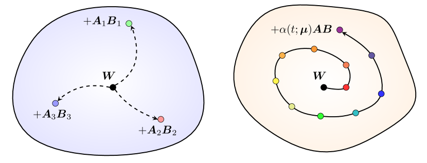
Our contribution: nonlinear reduced modeling with continuous low-rank adaptation (CoLoRA)
In this work, we build on LoRA (Low Rank Adaptation) for developing parameterizations for reduced models [41]. LoRA has been developed for fine-tuning large language models and leverages the observation that fine-tuning objectives can be efficiently optimized on low-dimensional parameter spaces [60, 1, 41]. This has been observed not only for large language models but also when approximating solution fields of physical phenomena [7, 37, 10]. We build on the pre-training/fine-tuning paradigm of LoRA but modify it to Continuous LoRA (CoLoRA) that reflects our PDE setting by allowing continuous-in-time adaptation (“fine-tuning”) of parts of the low-rank components as the solution fields of the PDEs evolve; see Figure 1. This inductive bias is in agreement with how typically physical phenomena evolve over time, namely smoothly and along a latent low-dimensional structure. By composing multiple CoLoRA layers in a deep network, we obtain a nonlinear parameterization that can circumvent the Kolmogorov barrier while having a pre-training/fine-tuning decomposition with an inductive bias that reflects the special meaning of the time variable in PDE problems; see Figure 2.
The time variable in CoLoRA models
Time enters CoLoRA models via the low-rank network weights that are adapted in the online (“fine-tuning”) phase of reduced modeling, rather than as input to the network as the spatial coordinates. Treating time separately from inputs such as the spatial coordinates aligns well with approximating PDE solution fields sequentially in time, rather than globally over the whole time-space domain. The sequential-in-time approximation paradigm of CoLoRA allows keeping the number of offline and online parameters low, because the solution field is approximated only locally in time. Requiring a low number of online and offline parameters indicates that the inductive bias induced by separating out the time variable from the spatial coordinate is in agreement with many physics problems. Furthermore, the CoLoRA architecture can be trained on low numbers of training trajectories compared to, e.g., operator learning [61, 62], which is important because standard numerical simulations can be expensive and thus only a limited number of training trajectories are available in many cases. Having network weights that depend on time allows combining CoLoRA with equation-driven variational approaches [55, 25, 4, 15] to obtain reduced solutions that are Galerkin-optimal, which opens the door to analyses, error bounds, and goes far beyond purely data-driven forecasting.
Literature review
There are purely data-driven surrogate modeling methods such as operator learning [61, 62, 13] that can require large amounts of data because they aim to learn a generic operator map over the full model space. Model reduction [5, 84, 9, 6, 54] considers a more structured problem via the physics parameter , for which nonlinear model reduction methods based on autoencoders have been presented in [56, 57, 50, 82]; however, they can require going back to the the high-fidelity numerical model to drive the dynamics, which can be expensive. Alternative approaches learn the low-dimensional latent dynamics [32, 58, 93]. Additional literature of nonlinear model reduction is reviewed in Appendix A. There is a range of methods based on implicit neural representations that updates the network parameters either based on the equation [18, 19] or via hyper-networks [71, 96]; these methods are closest to CoLoRA, except that we will show that the CoLoRA’s low-rank adaptation achieves lower errors with lower parameter counts in our examples. There are pre-training/fine-tuning techniques for global-in-time methods such as physics-informed neural networks [78] that are purely data-driven once trained. Some of these approaches use hyper-networks [22, 20] and other meta-learning such as [30]. But typically these approaches are over time-space domains and thus do not make a special treatment of time or the PDE dynamics, which is a key feature of CoLoRA. Adaptive low-rank approximations have been used in scientific computing for a long time [53, 86, 29]; however, they use one layer only and adapt the low-rank matrices directly with time. We have a more restricted adaptation in time that has fewer parameters, which is sufficient due to the non-linear composition of multiple layers. Other low-rank approximations have been widely used in the context of deep networks [85, 98, 99, 48, 87] but not in PDE settings.
Summary
CoLoRA leverages that PDE dynamics are typically continuous in time while evolving on low-dimensional manifolds. With CoLoRA, we achieve nonlinear parameterizations that circumvent the Kolmogovorv barrier of transport-dominated problems and can provide predictions purely data-driven or in a variational sense using the PDEs. Our numerical experiments show that CoLoRA requires a low number of training trajectories, achieves orders of magnitude speedups compared to classical methods, and outperforms the existing state-of-the-art neural-network-based model reduction methods in parameter count and accuracy on a wide variety of PDE problems.
2 Parameterized PDEs
Let be a solution field that represents, e.g., temperature, density, velocities, or pressure of a physical process. The solution field depends on time , spatial coordinate , and physics parameter . The solution field is governed by a parameterized PDE,
| (1) | |||||
where is the initial condition and can include partial derivatives of in . In the following, we always have appropriate boundary conditions so that the PDE problem (1) is well posed. The physics parameter can enter the dynamics via and the initial condition . Standard numerical methods such as finite-element [43] and finite-volume [59] methods can be used to numerically solve (1) to obtain a numerical solution for a physics parameter .
Computational procedures for learning reduced models [5, 84, 9, 6, 54] are typically split into an offline and an online phase: In the offline (training) phase, the reduced model is constructed from training trajectories
| (2) |
over offline physics parameters , which have been computed with the high-fidelity numerical model. In the subsequent online phase, the reduced model is used to rapidly predict solution fields at new physics parameters and initial conditions.
3 CoLoRA networks
We introduce CoLoRA deep networks that (a) provide nonlinear parameterizations that circumvent the Kolmogorov barrier of linear model reduction and (b) impose an inductive bias that treats the time variable differently from the spatial variable , which reflects that time is a special variable in physics. In particular, CoLoRA networks allow a continuous adaptation of a low number of network weights over time to capture the dynamics of solution fields (“fine-tuning”) for different physics parameters.
3.1 LoRA layers
CoLoRA networks are motivated by LoRA [41], a method that has been introduced to fine-tune large language models on discrete downstream tasks. LoRA layers are defined as
| (3) |
where is the input vector, are weight matrices, and is the bias term. The key of LoRA is that only is changed during fine tuning and that is of low rank so it can be parameterized as,
Thus, only parameters need to be update per layer during fine-tuning rather than all as during pre-training,
3.2 The CoLoRA layer
Models with low intrinsic dimension are very common not only in large language models but also in many applications in science and engineering with phenomena that are described by PDEs [7, 37, 10]. However, in the PDE settings, we have the special time variable that requires us to “fine-tune” continuously as the PDE solution trajectories evolve; see Figure 1. Additionally, time imposes causality, which we want to preserve in CoLoRA models.
To enable a continuous low-rank adaptation, we introduce Continuous LoRA (CoLoRA) layers,
| (4) |
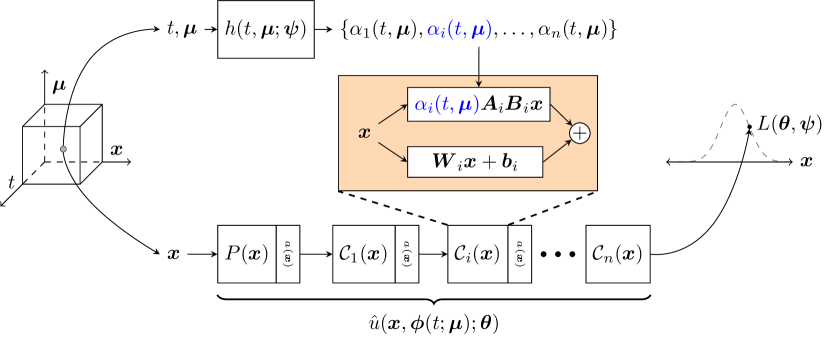
where is a low-rank matrix of rank that is trained offline and is the online (“fine-tuning”) parameter that can change continuously with and also with the physics parameter in the online phase of model reduction. For example, when using a multilayer perceptron (MLP) with -many layers and a linear output layer , we obtain
| (5) |
with activation function and for . The online parameters are given by the vector with in the example (5). We will later refer to as the latent state. All other CoLoRA parameters that are independent of time and physics parameter are trainable offline and collected into the offline parameter vector of dimension .
We note in principle could be full rank without increasing the size of . But this would increase the number of parameters in . Additionally, the authors of LoRA [41] observed that full rank fine-tuning updates under-perform low rank ones despite having more degrees of freedom, which is also in agreement with the very low ranks used in dynamic low-rank and online adaptive methods in model reduction [53, 86, 29, 73, 76, 89].
A CoLoRA network defines a function that depends on an input , which is the spatial coordinate in our PDE setting, the offline parameters that are independent of time and physics parameter and the online parameters or latent state that depends on and . A CoLoRA network can also output more than one quantity by modifying the output layer, which we will use for approximating systems of PDEs in the numerical experiments. A CoLoRA network is a implicit neural representation [90, 71] in the sense that the PDE solution field is given implicitly by the parameters and and it can be evaluated at any coordinate , irrespective of discretizations and resolutions used during training.
If is a scalar for each layer , then the dimension of equals the number of layers in in the MLP example (5), which can be overly restrictive. So we additional allow to have -many online parameters for each layer, in which case we have The dimension of the online parameter vector is then . Other approaches are possible to make CoLoRA networks more expressive such as allowing and to depend on and as well; however, as we will show with our numerical experiments, only very few online parameters are needed in our experiments.
3.3 CoLoRA networks can circumvent the Kolmogorov barrier
CoLoRA networks can be nonlinear in the online parameter and thus can achieve faster error decays than given by (linear) Kolmogorov -widths. We give one example by considering the linear advection equation as in [70] with initial condition and solution , which can lead to a slow -width decay of for a linear parameterization with parameters. In contrast, with the CoLoRA MLP network with layers, we can exactly represent translation and thus the solution of the linear advection equation: Set and arbitrary. Further and and . If we use the known initial condition as activation function and the identity as activation function and set , then we obtain , which is the solution of the linear advection example above. Of course this is a contrived example but it shows how translation can be represented well by CoLoRA networks, which is the challenge that leads to the Kolmogorov barrier [74]. A more detailed treatment of the approximation theoretic properties of CoLoRA networks remains an open theory question that we leave for future work.
4 Training CoLoRA models offline
The goal of the following training procedure is to learn the offline parameters of a CoLoRA network for a given parameterized PDE (1) so that only the much lower dimensional latent state has to be updated online over time and physics parameters to approximate well the solution of the PDE.
Enforcing continuity in time
CoLoRA models make a careful treatment of time , which enters via the latent state rather than as input as the spatial coordinates ; see also the discussion in Section 1. We want that special meaning of the time variable to be also reflected in the pre-training approach in the sense of imposing regularity in the latent state with respect to time . Having smooth latent dynamics is a key property that has many desirable outcomes such as rapid time-stepping with large time step sizes, stability, and robustness to numerical perturbations. A naive pre-training of CoLoRA over and with a global optimization problem would allow to change arbitrarily, i.e., in a non-smooth way, over time.
To impose regularity with respect to , we introduce a hyper-network that depends on the parameter vector ; see [22, 71, 20] for other methods that build on hyper-networks in different settings. Time and physics parameter are inputs to the hyper-network and is the output. We focus on the case where is an MLP, but we stress that any other regression model can be used that provides the necessary regularity from to . For our purposes here, it is sufficient to choose such that it is continuous in . This means that its output written as will depend continuously on time .
Loss function for pre-training
Recall that we have access to training data in the form of solution fields for given in (2). For , we consider finite sets and of spatial coordinates and time samples over the spatial domain and time domain, respectively. For each offline physics parameter , we consider the relative error over the cross product
where denotes the training trajectory for that is available from the high-fidelity numerical model, is our CoLoRA parameterizations, and is the hyper-network discussed in the previous paragraph.
The loss that we optimize for the offline parameters and the parameter vector of the hyper-network averages the relative errors over all training physics parameters,
| (6) |
This is also the mean relative error that we report on test parameters in our experiments; see Section 6.
We stress that in the spirit of implicit neural representations, the pre-training (as well as online) approach is independent of grids in the spatial and time domain. In fact, our formulation via the sets and for each training physics parameter allows for different, unstructured samples in the spatial and time domain for each training physics parameter.
5 Online phase of CoLoRA models
Given a new parameter that we have not seen during training, the goal of the online phase is to rapidly approximate the high-fidelity numerical solution at . With pre-trained CoLoRA models, we can go about this in two fundamentally different ways: First, we can take a purely data-driven route and simply evaluate the hyper-network at the new at any time . Second, because the latent state depends on time , we can take an equation-driven route and use the governing equation given in (1) to derive the online parameter via a variational formulation such as Neural Galerkin schemes [15]; see [55, 25, 4, 10] for other sequential-in-time methods that could be combined with CoLoRA.
5.1 Data-driven forecasting (CoLoRA-D)
We refer to CoLoRA models as CoLoRA-D if predictions at a new physics parameter are obtained by evaluating the hyper-network at and the times of interest. The predictions that are obtained from CoLoRA-D models are purely data-driven and therefore do not directly use the governing equations in any way; neither during the pre-training nor during the online phase. Reduced models based on CoLoRA-D are non-intrusive [36, 54], which can have major advantages in terms of implementation and deployment because only data needs to be available; these advantages are the same as for operator learning [61, 62] that also is non-intrusive and typically relies only on data rather than the governing equations. The accuracy of CoLoRA-D models, however, critically depends on the generalization of , which is in agreement with data-driven forecasting in general that has to rely alone on the generalization of data-fitted functions.
5.2 Equation-driven predictions (CoLoRA-EQ)
If the governing equations given in (1) are available, they can be used together with CoLoRA models to compute the states for a new parameter in a variational sense. We follow Neural Galerkin schemes [15], which provide a method for solving for parameters that enter non-linearly so that the corresponding parameterizations, in a variational sense, solve the given PDE. We stress that such a variational formulation is possible with CoLoRA models because the latent state depends on time rather than time being an input as the spatial coordinate . In particular, the sequential-in-time training of Neural Galerkin schemes is compatible with the time-dependent online parameter . Together with Neural Galerkin schemes, CoLoRA provide solutions that are causal, which is different from many purely data-driven methods.
Neural Galerkin schemes build on the Dirac-Frenkel variational principle [24, 31, 63, 55], which can be interpreted as finding time derivatives that solve the Galerkin condition
so that the residual of the PDE (1) as a function over the spatial domain is orthogonal to the tangent space of the manifold induced by the online parameters at the current function ; we refer to [15] for details and to Appendix H for the computational procedure.
The key feature of the equation-driven approach for predictions with CoLoRA models is that the latent states are optimal in a Galerkin sense, which provides a variational interpretation of the solution and opens the door to using residual-based error estimators to provide accuracy guarantees, besides other theory tools. Additionally, as mentioned above, it imposes causality, which is a fundamental principle in science that we often want to preserve in numerical simulations. Furthermore, using the governing equations is helpful to conserve quantities such as energy, mass, momentum, which we will demonstrate in Section 6.6.
6 Numerical experiments
6.1 PDE problems
The following three problems are challenging to reduce with conventional linear model reduction methods because the dynamics are transport dominated [74]. Additional details on these equations and the full order models are provided in Appendix C.
Collisionless charged particles in electric field
The Vlasov equation describes the motion of collisionless charged particles under the influence of an electric field. We consider the setup of [39], which demonstrates filamentation of the distribution function of charged particles as they are affected by the electric field. Our physics parameter enters via the initial condition. The full numerical model benchmarked in Figure 4 uses second-order finite differences on a grid with adaptive time integrator.
Burgers’ equation in 2D
Fields governed by the Burgers’ equations can form sharp advecting fronts. The sharpness of these fronts are controlled by the viscosity parameter which we use as our physics parameter . The full model benchmarked in Figure 4 uses 2nd-order finite differences and a spatial grid with an implicit time integration scheme using a time step size of .
Rotating denotation waves We consider a model of rotating detonation waves, which is motivated by space propulsion with rotating detonation engines (RDE) [52, 3, 79]. The equations describe the time evolution of the intensive property of the working fluid and the combustion progress. The physics parameter we reduce over corresponds to the combustion injection rate, which leads to bifurcation phenomena that we investigate over the interval ; see C.3 for details. The full model benchmarked in Figure 4 uses a finite volume method on a grid with an implicit time integration scheme using a time step size of .
Other PDE models We also look at other PDEs to benchmark against methods from the literature; see Table 1. These include a two-dimensional wave problem with a four-dimensional physics parameter.
6.2 CoLoRA architectures
The reduced-model parameterization is an MLP with CoLoRA layers. The hyper-network is an MLP with regular linear layers. Both use swish activation functions. The most important architectural choice we make is the size of our networks— has 8 layers each of width 25 and has three layers each of width 15. As discussed earlier, such small networks are sufficient because of the strong inductive bias and low-rank continuity in time of CoLoRA networks. The error metric we report is the mean relative error, which is also our loss function (6). All additional choices regarding the architecture, training and data sampling are detailed in Appendix D and Figure 7.
6.3 CoLoRA and number of latent parameters
Figure 3 compares the mean relative error of the proposed CoLoRA models with conventional linear projections, which serve as the empirical best-approximation error that can be achieved with any linear model reduction method (see Appendix F). In all examples, the error is shown for test physics parameters that have not been used during training; see Appendix G.
First, the linear approximations are ineffective for all three examples, which is in agreement with the observation from Section 6.1 that the three PDE models are challenging to reduce with linear model reduction methods. Second, our CoLoRA models achieve orders of magnitude lower relative errors for the same number of parameters as linear approximations. In all examples, 2–3 latent parameters are sufficient in CoLoRA models, which is in agreement with the low dimensionality of the physics parameters of these models. After the steep drop off of the error until around online parameters, there is a slow improvement if any as we increase , which is in agreement with other nonlinear approximations methods [19, 56]. This is because once is equal to the intrinsic dimension of the problem, compression no longer helps reduce errors in predictions and instead the error is driven by other error sources such as time integration and generalization of the hyper-network. In these examples, the purely data-driven CoLoRA-D achieves slightly lower relative errors than the equation-driven CoLoRA-EQ, which could be due to the time integration error. In any case, the CoLoRA-EQ results show that we learn representations that are consistent with the PDE dynamics in the Dirac-Frenkel variational sense.
6.4 Speedups of CoLoRA
In Figure 4, we show the relative speedup of CoLoRA when compared to the runtime of the high-fidelity numerical models based on finite-difference and finite-volume methods as described in Appendix C. The speedups in the Burgers’ and the RDE examples are higher than in the Vlasov example because we use an explicit time integration scheme for Vlasov but implicit ones for Burgers’ and RDE. When integrating the governing equations in CoLoRA-EQ, we achieve speedups because of the smoothness of the latent dynamics of as shown in Figure 2. The smoothness allows us to integrate with a solver that uses an adaptive time-step control, which adaptively selects large time steps due to the smoothness of the dynamics. When using CoLoRA-D, we achieve orders of magnitude higher speedups because forecasting requires evaluating the hyper-network only. This can be done quickly due to the small size of the hyper-network as described in Section 6.2. We note that we benchmark our method on the time it takes to compute the latent state on the same time grid as the full model. There will of course be additional computational costs associated with plotting the CoLoRA solution on a grid in .
6.5 Data efficiency versus operator learning
A key difference to operator learning is that CoLoRA aims to predict well the influence of the physics parameter on the solution fields, rather than aiming for a generic operator that maps a solution at one time step to the next. We now show that CoLoRA can leverage the more restrictive problem formulation so that fewer training trajectories are sufficient. As Figure 4 shows for the Burgers’ and Vlasov example, we achieve relative errors in the range of with only about training trajectories, whereas the operator- learning variant F-FNO [92] based on Fourier neural operators (FNOs) [61] leads to an about one order of magnitude higher relative error. Neural operators struggle to achieve relative errors below , while CoLoRA achieves one order of magnitude lower relative errors with one order of magnitude fewer training trajectories. We also compare to simply linearly interpolating the function over space, time, and parameter and observe that in low data regimes CoLoRA achieves orders of magnitude more accurate predictions. In high data regimes, for sufficiently smooth problems, linear interpolation will become very accurate as training physics parameters start to be closer and closer to test physics parameters; see Appendix G for details.
6.6 Leveraging physics knowledge in the online phase with CoLoRA-EQ
In the numerical experiments conducted so far, the purely data-driven CoLoRA-D outperforms CoLoRA-EQ in terms of error and speedup. However, using the physics equations online can be beneficial in other ways such as for causality and theoretical implications, especially for residual-based error estimators; see Section 5. We now discuss another one here numerically, namely conserving quantities during time integration.
We build on conserving Neural Galerkin schemes introduced in [88] to conserve the mass of the probability distribution that describes the particles in the Vlasov problem. Preserving unit mass can be important for physics interpretations. In Figure 5, we show that using the CoLoRA-EQ with [88], we are able to conserve the mass of solution fields of the Vlasov equation to machine precision. By contrast, neither the CoLoRA-D nor F-FNO conserve the quantity, as the numerical experiments show.
6.7 Comparison to other nonlinear methods
| PDE | method | rel. err | param | |
|---|---|---|---|---|
| 2D Wave | DINo | 6.89e-3 | 50 | |
| 2D Wave | CoLoRA-D | 9.22e-4 | 7505 | 49 |
| 1D Burg. | CROM | 1.93e-3 | 19470 | 2 |
| 1D Burg. | CoLoRA-D | 2.74e-04 | 4521 | 2 |
| Vlasov | F-FNO | 8.57e-3 | - | |
| Vlasov | CoLoRA-D | 9.87e-04 | 5451 | 7 |
| 2D Burg. | F-FNO | 5.11e-3 | - | |
| 2D Burg. | CoLoRA-D | 4.96e-04 | 5451 | 7 |
We run CoLoRA on the 2D wave benchmark problem described in the DINo publication [96]; see Table 1. CoLoRA achieves an about one order of magnitude lower error than DINo while using about one order of magnitude fewer parameters. We also compare CoLoRA against CROM [19], another nonlinear reduce modeling method that uses neural networks. We benchmark our method against the 1D inviscid Burgers’ problem that the authors of CROM describe in their publication [19]. CoLoRA achieves an about one order of magnitude lower error than CROM, again using about one order of magnitude fewer parameters.
7 Conclusions
CoLoRA leverages that PDE dynamics are typically continuous in time while evolving on low-dimensional manifolds. CoLoRA models provide nonlinear approximations and therefore are efficient in reducing transport-dominated problems that are affected by the Kolmogorov barrier. At the same time, CoLoRA is data efficient and requires only few training trajectories in our examples. The continuous-in-time adaptation of CoLoRA network weights leads to rapid predictions of solution fields of PDEs at new physics parameters, which outperforms current state-of-the-art methods. We provide an implementation of CoLoRA at https://github.com/julesberman/CoLoRA.
Acknowledgements
The authors were partially supported by the National Science Foundation under Grant No. 2046521 and the Office of Naval Research under award N00014-22-1-2728. This work was also supported in part through the NYU IT High Performance Computing resources, services, and staff expertise.
References
- [1] A. Aghajanyan, S. Gupta, and L. Zettlemoyer. Intrinsic dimensionality explains the effectiveness of language model fine-tuning. In C. Zong, F. Xia, W. Li, and R. Navigli, editors, Proceedings of the 59th Annual Meeting of the Association for Computational Linguistics and the 11th International Joint Conference on Natural Language Processing (Volume 1: Long Papers), pages 7319–7328, Online, Aug. 2021. Association for Computational Linguistics.
- [2] D. Amsallem, M. J. Zahr, and C. Farhat. Nonlinear model order reduction based on local reduced-order bases. International Journal for Numerical Methods in Engineering, 92(10):891–916, 2012.
- [3] V. Anand and E. Gutmark. Rotating detonation combustors and their similarities to rocket instabilities. Progress in Energy and Combustion Science, 73:182–234, 2019.
- [4] W. Anderson and M. Farazmand. Evolution of nonlinear reduced-order solutions for PDEs with conserved quantities. SIAM Journal on Scientific Computing, 44(1):A176–A197, 2022.
- [5] A. C. Antoulas. Approximation of large-scale dynamical systems. SIAM, 2005.
- [6] A. C. Antoulas, C. A. Beattie, and S. Gugercin. Interpolatory Methods for Model Reduction. SIAM, 2021.
- [7] M. Bachmayr, A. Cohen, and W. Dahmen. Parametric PDEs: sparse or low-rank approximations? IMA Journal of Numerical Analysis, 38(4):1661–1708, 09 2017.
- [8] J. Barnett and C. Farhat. Quadratic approximation manifold for mitigating the Kolmogorov barrier in nonlinear projection-based model order reduction. Journal of Computational Physics, 464:111348, 2022.
- [9] P. Benner, S. Gugercin, and K. Willcox. A survey of projection-based model reduction methods for parametric dynamical systems. SIAM review, 57(4):483–531, 2015.
- [10] J. Berman and B. Peherstorfer. Randomized sparse Neural Galerkin schemes for solving evolution equations with deep networks. In Thirty-seventh Conference on Neural Information Processing Systems, 2023.
- [11] M. Billaud-Friess and A. Nouy. Dynamical model reduction method for solving parameter-dependent dynamical systems. SIAM Journal on Scientific Computing, 39(4):A1766–A1792, 2017.
- [12] Black, Felix, Schulze, Philipp, and Unger, Benjamin. Projection-based model reduction with dynamically transformed modes. ESAIM: M2AN, 54(6):2011–2043, 2020.
- [13] N. Boullé and A. Townsend. A Mathematical Guide to Operator Learning, Dec. 2023. arXiv:2312.14688 [cs, math].
- [14] J. Bradbury, R. Frostig, P. Hawkins, M. J. Johnson, C. Leary, D. Maclaurin, G. Necula, A. Paszke, J. VanderPlas, S. Wanderman-Milne, and Q. Zhang. JAX: composable transformations of Python+NumPy programs. 2018.
- [15] J. Bruna, B. Peherstorfer, and E. Vanden-Eijnden. Neural Galerkin schemes with active learning for high-dimensional evolution equations. Journal of Computational Physics, 496:112588, Jan. 2024.
- [16] N. Cagniart, Y. Maday, and B. Stamm. Model order reduction for problems with large convection effects. In B. N. Chetverushkin, W. Fitzgibbon, Y. Kuznetsov, P. Neittaanmäki, J. Periaux, and O. Pironneau, editors, Contributions to Partial Differential Equations and Applications, pages 131–150, Cham, 2019. Springer International Publishing.
- [17] K. Carlberg. Adaptive h-refinement for reduced-order models. International Journal for Numerical Methods in Engineering, 102(5):1192–1210, 2015.
- [18] H. Chen, R. Wu, E. Grinspun, C. Zheng, and P. Y. Chen. Implicit neural spatial representations for time-dependent PDEs. In A. Krause, E. Brunskill, K. Cho, B. Engelhardt, S. Sabato, and J. Scarlett, editors, Proceedings of the 40th International Conference on Machine Learning, volume 202 of Proceedings of Machine Learning Research, pages 5162–5177. PMLR, 23–29 Jul 2023.
- [19] P. Y. Chen, J. Xiang, D. H. Cho, Y. Chang, G. A. Pershing, H. T. Maia, M. M. Chiaramonte, K. T. Carlberg, and E. Grinspun. CROM: Continuous reduced-order modeling of PDEs using implicit neural representations. In The Eleventh International Conference on Learning Representations, 2023.
- [20] W. Cho, K. Lee, D. Rim, and N. Park. Hypernetwork-based meta-learning for low-rank physics-informed neural networks. In Thirty-seventh Conference on Neural Information Processing Systems, 2023.
- [21] A. Cohen and R. DeVore. Kolmogorov widths under holomorphic mappings. IMA J. Numer. Anal., 36(1):1–12, 2016.
- [22] F. de Avila Belbute-Peres, Y. fan Chen, and F. Sha. HyperPINN: Learning parameterized differential equations with physics-informed hypernetworks. In The Symbiosis of Deep Learning and Differential Equations, 2021.
- [23] M. Dihlmann, M. Drohmann, and B. Haasdonk. Model reduction of parametrized evolution problems using the reduced basis method with adaptive time-partitioning. In Proc. of ADMOS 2011, 2011.
- [24] P. A. M. Dirac. Note on exchange phenomena in the thomas atom. Mathematical Proceedings of the Cambridge Philosophical Society, 26(3):376–385, 1930.
- [25] Y. Du and T. A. Zaki. Evolutional deep neural network. Physical Review E, 104(4), Oct. 2021.
- [26] J. L. Eftang and B. Stamm. Parameter multi-domain ‘hp’ empirical interpolation. International Journal for Numerical Methods in Engineering, 90(4):412–428, 2012.
- [27] V. Ehrlacher, D. Lombardi, O. Mula, and F.-X. Vialard. Nonlinear model reduction on metric spaces. Application to one-dimensional conservative PDEs in Wasserstein spaces. ESAIM Math. Model. Numer. Anal., 54(6):2159–2197, 2020.
- [28] L. Einkemmer, J. Hu, and Y. Wang. An asymptotic-preserving dynamical low-rank method for the multi-scale multi-dimensional linear transport equation. Journal of Computational Physics, 439:110353, 2021.
- [29] L. Einkemmer and C. Lubich. A quasi-conservative dynamical low-rank algorithm for the vlasov equation. SIAM Journal on Scientific Computing, 41(5):B1061–B1081, 2019.
- [30] C. Finn, P. Abbeel, and S. Levine. Model-agnostic meta-learning for fast adaptation of deep networks. In D. Precup and Y. W. Teh, editors, Proceedings of the 34th International Conference on Machine Learning, volume 70 of Proceedings of Machine Learning Research, pages 1126–1135. PMLR, 06–11 Aug 2017.
- [31] J. Frenkel. Wave Mechanics, Advanced General Theor. Clarendon Press, Oxford, 1934.
- [32] L. Fulton, V. Modi, D. Duvenaud, D. I. W. Levin, and A. Jacobson. Latent-space dynamics for reduced deformable simulation. Computer Graphics Forum, 2019.
- [33] R. Geelen and K. Willcox. Localized non-intrusive reduced-order modelling in the operator inference framework. Philosophical Transactions of the Royal Society A: Mathematical, Physical and Engineering Sciences, 380(2229):20210206, 2022.
- [34] R. Geelen, S. Wright, and K. Willcox. Operator inference for non-intrusive model reduction with quadratic manifolds. Computer Methods in Applied Mechanics and Engineering, 403:115717, 2023.
- [35] J.-F. Gerbeau and D. Lombardi. Approximated lax pairs for the reduced order integration of nonlinear evolution equations. Journal of Computational Physics, 265:246–269, 2014.
- [36] O. Ghattas and K. Willcox. Learning physics-based models from data: perspectives from inverse problems and model reduction. Acta Numerica, 30:445–554, 2021.
- [37] L. Grasedyck, D. Kressner, and C. Tobler. A literature survey of low-rank tensor approximation techniques. GAMM-Mitteilungen, 36(1):53–78, 2013.
- [38] C. Greif and K. Urban. Decay of the Kolmogorov N-width for wave problems. Applied Mathematics Letters, 96:216–222, 2019.
- [39] Y. Güçlü, A. J. Christlieb, and W. N. Hitchon. Arbitrarily high order convected scheme solution of the vlasov–poisson system. Journal of Computational Physics, 270:711–752, Aug. 2014.
- [40] J. S. Hesthaven, C. Pagliantini, and G. Rozza. Reduced basis methods for time-dependent problems. Acta Numerica, 31:265–345, 2022.
- [41] E. J. Hu, yelong shen, P. Wallis, Z. Allen-Zhu, Y. Li, S. Wang, L. Wang, and W. Chen. LoRA: Low-rank adaptation of large language models. In International Conference on Learning Representations, 2022.
- [42] C. Huang and K. Duraisamy. Predictive reduced order modeling of chaotic multi-scale problems using adaptively sampled projections. Journal of Computational Physics, 491:112356, 2023.
- [43] T. J. R. Hughes. The Finite Element Method: Linear Static and Dynamic Finite Element Analysis. Dover Publications, 2012.
- [44] A. Iollo and D. Lombardi. Advection modes by optimal mass transfer. Phys. Rev. E, 89:022923, Feb 2014.
- [45] O. Issan and B. Kramer. Predicting solar wind streams from the inner-heliosphere to earth via shifted operator inference. Journal of Computational Physics, 473:111689, 2023.
- [46] D. J. K. Jens L. Eftang and A. T. Patera. An hp certified reduced basis method for parametrized parabolic partial differential equations. Mathematical and Computer Modelling of Dynamical Systems, 17(4):395–422, 2011.
- [47] S. Kaulmann, B. Flemisch, B. Haasdonk, K. A. Lie, and M. Ohlberger. The localized reduced basis multiscale method for two-phase flows in porous media. International Journal for Numerical Methods in Engineering, 102(5):1018–1040, 2015.
- [48] M. Khodak, N. A. Tenenholtz, L. Mackey, and N. Fusi. Initialization and regularization of factorized neural layers. In International Conference on Learning Representations, 2021.
- [49] C. Kim, D. Lee, S. Kim, M. Cho, and W.-S. Han. Generalizable Implicit Neural Representations via Instance Pattern Composers. In 2023 IEEE/CVF Conference on Computer Vision and Pattern Recognition (CVPR), pages 11808–11817, Vancouver, BC, Canada, June 2023. IEEE.
- [50] Y. Kim, Y. Choi, D. Widemann, and T. Zohdi. A fast and accurate physics-informed neural network reduced order model with shallow masked autoencoder. Journal of Computational Physics, 451:110841, 2022.
- [51] D. P. Kingma and J. Ba. Adam: A method for stochastic optimization, 2017.
- [52] J. Koch, M. Kurosaka, C. Knowlen, and J. N. Kutz. Mode-locked rotating detonation waves: Experiments and a model equation. Physical Review E, 101(1), Jan. 2020.
- [53] O. Koch and C. Lubich. Dynamical low-rank approximation. SIAM Journal on Matrix Analysis and Applications, 29(2):434–454, 2007.
- [54] B. Kramer, B. Peherstorfer, and K. E. Willcox. Learning nonlinear reduced models from data with operator inference. Annual Review of Fluid Mechanics, 56(1):521–548, 2024.
- [55] C. Lasser and C. Lubich. Computing quantum dynamics in the semiclassical regime. Acta Numerica, 29:229–401, 2020.
- [56] K. Lee and K. T. Carlberg. Model reduction of dynamical systems on nonlinear manifolds using deep convolutional autoencoders. Journal of Computational Physics, 404:108973, 2020.
- [57] K. Lee and K. T. Carlberg. Deep conservation: A latent-dynamics model for exact satisfaction of physical conservation laws. Proceedings of the AAAI Conference on Artificial Intelligence, 35(1):277–285, May 2021.
- [58] K. Lee and E. J. Parish. Parameterized neural ordinary differential equations: applications to computational physics problems. Proceedings of the Royal Society A: Mathematical, Physical and Engineering Sciences, 477(2253):20210162, 2021.
- [59] R. J. LeVeque. Finite Volume Methods for Hyperbolic Problems. Cambridge Texts in Applied Mathematics. Cambridge University Press, 2002.
- [60] C. Li, H. Farkhoor, R. Liu, and J. Yosinski. Measuring the intrinsic dimension of objective landscapes. In International Conference on Learning Representations, 2018.
- [61] Z. Li, N. B. Kovachki, K. Azizzadenesheli, B. liu, K. Bhattacharya, A. Stuart, and A. Anandkumar. Fourier neural operator for parametric partial differential equations. In International Conference on Learning Representations, 2021.
- [62] L. Lu, P. Jin, G. Pang, Z. Zhang, and G. E. Karniadakis. Learning nonlinear operators via deeponet based on the universal approximation theorem of operators. Nature Machine Intelligence, 3(3):218–229, Mar 2021.
- [63] C. Lubich. From quantum to classical molecular dynamics: reduced models and numerical analysis, volume 12. European Mathematical Society, 2008.
- [64] Y. Maday, A. T. Patera, and G. Turinici. Global a priori convergence theory for reduced-basis approximations of single-parameter symmetric coercive elliptic partial differential equations. C. R. Math. Acad. Sci. Paris, 335(3):289–294, 2002.
- [65] Y. Maday and B. Stamm. Locally adaptive greedy approximations for anisotropic parameter reduced basis spaces. SIAM Journal on Scientific Computing, 35(6):A2417–A2441, 2013.
- [66] E. Musharbash and F. Nobile. Symplectic dynamical low rank approximation of wave equations with random parameters. Mathicse Technical Report nr 18.2017, 2017.
- [67] E. Musharbash and F. Nobile. Dual dynamically orthogonal approximation of incompressible Navier Stokes equations with random boundary conditions. Journal of Computational Physics, 354:135 – 162, 2018.
- [68] E. Musharbash, F. Nobile, and T. Zhou. Error analysis of the dynamically orthogonal approximation of time dependent random pdes. SIAM Journal on Scientific Computing, 37(2):A776–A810, 2015.
- [69] M. Ohlberger and S. Rave. Nonlinear reduced basis approximation of parameterized evolution equations via the method of freezing. Comptes Rendus Mathematique, 351(23):901 – 906, 2013.
- [70] M. Ohlberger and S. Rave. Reduced basis methods: Success, limitations and future challenges. Proceedings of the Conference Algoritmy, pages 1–12, 2016.
- [71] S. Pan, S. L. Brunton, and J. N. Kutz. Neural implicit flow: a mesh-agnostic dimensionality reduction paradigm of spatio-temporal data. Journal of Machine Learning Research, 24(41):1–60, 2023.
- [72] D. Papapicco, N. Demo, M. Girfoglio, G. Stabile, and G. Rozza. The neural network shifted-proper orthogonal decomposition: A machine learning approach for non-linear reduction of hyperbolic equations. Computer Methods in Applied Mechanics and Engineering, 392:114687, 2022.
- [73] B. Peherstorfer. Model reduction for transport-dominated problems via online adaptive bases and adaptive sampling. SIAM Journal on Scientific Computing, 42:A2803–A2836, 2020.
- [74] B. Peherstorfer. Breaking the Kolmogorov barrier with nonlinear model reduction. Notices of the American Mathematical Society, 69:725–733, 2022.
- [75] B. Peherstorfer, D. Butnaru, K. Willcox, and H.-J. Bungartz. Localized discrete empirical interpolation method. SIAM Journal on Scientific Computing, 36(1):A168–A192, 2014.
- [76] B. Peherstorfer and K. Willcox. Online adaptive model reduction for nonlinear systems via low-rank updates. SIAM Journal on Scientific Computing, 37(4):A2123–A2150, 2015.
- [77] E. Qian, B. Kramer, B. Peherstorfer, and K. Willcox. Lift & learn: Physics-informed machine learning for large-scale nonlinear dynamical systems. Physica D: Nonlinear Phenomena, 406:132401, 2020.
- [78] M. Raissi, P. Perdikaris, and G. Karniadakis. Physics-informed neural networks: A deep learning framework for solving forward and inverse problems involving nonlinear partial differential equations. Journal of Computational Physics, 378:686–707, 2019.
- [79] V. Raman, S. Prakash, and M. Gamba. Nonidealities in rotating detonation engines. Annual Review of Fluid Mechanics, 55(1):639–674, 2023.
- [80] D. Ramezanian, A. G. Nouri, and H. Babaee. On-the-fly reduced order modeling of passive and reactive species via time-dependent manifolds. Computer Methods in Applied Mechanics and Engineering, 382:113882, 2021.
- [81] J. Reiss, P. Schulze, J. Sesterhenn, and V. Mehrmann. The shifted proper orthogonal decomposition: a mode decomposition for multiple transport phenomena. SIAM J. Sci. Comput., 40(3):A1322–A1344, 2018.
- [82] F. Romor, G. Stabile, and G. Rozza. Non-linear manifold reduced-order models with convolutional autoencoders and reduced over-collocation method. Journal of Scientific Computing, 94(3):74, Feb 2023.
- [83] C. W. Rowley and J. E. Marsden. Reconstruction equations and the Karhunen–Loève expansion for systems with symmetry. Physica D: Nonlinear Phenomena, 142(1):1–19, 2000.
- [84] G. Rozza, D. B. P. Huynh, and A. T. Patera. Reduced basis approximation and a posteriori error estimation for affinely parametrized elliptic coercive partial differential equations. Archives of Computational Methods in Engineering, 15(3):229–275, 2008.
- [85] T. N. Sainath, B. Kingsbury, V. Sindhwani, E. Arisoy, and B. Ramabhadran. Low-rank matrix factorization for deep neural network training with high-dimensional output targets. In 2013 IEEE International Conference on Acoustics, Speech and Signal Processing, pages 6655–6659, 2013.
- [86] T. P. Sapsis and P. F. Lermusiaux. Dynamically orthogonal field equations for continuous stochastic dynamical systems. Physica D: Nonlinear Phenomena, 238(23):2347–2360, 2009.
- [87] S. Schotthöfer, E. Zangrando, J. Kusch, G. Ceruti, and F. Tudisco. Low-rank lottery tickets: finding efficient low-rank neural networks via matrix differential equations. In S. Koyejo, S. Mohamed, A. Agarwal, D. Belgrave, K. Cho, and A. Oh, editors, Advances in Neural Information Processing Systems, volume 35, pages 20051–20063. Curran Associates, Inc., 2022.
- [88] P. Schwerdtner, P. Schulze, J. Berman, and B. Peherstorfer. Nonlinear embeddings for conserving Hamiltonians and other quantities with Neural Galerkin schemes, Oct. 2023. arXiv:2310.07485 [cs, math].
- [89] R. Singh, W. Uy, and B. Peherstorfer. Lookahead data-gathering strategies for online adaptive model reduction of transport-dominated problems. Chaos: An Interdisciplinary Journal of Nonlinear Science, 2023.
- [90] V. Sitzmann, J. N. P. Martel, A. W. Bergman, D. B. Lindell, and G. Wetzstein. Implicit neural representations with periodic activation functions, 2020.
- [91] T. Taddei, S. Perotto, and A. Quarteroni. Reduced basis techniques for nonlinear conservation laws. ESAIM Math. Model. Numer. Anal., 49(3):787–814, 2015.
- [92] A. Tran, A. Mathews, L. Xie, and C. S. Ong. Factorized Fourier Neural Operators, Mar. 2023. arXiv:2111.13802 [cs].
- [93] Z. Y. Wan, L. Zepeda-Nunez, A. Boral, and F. Sha. Evolve smoothly, fit consistently: Learning smooth latent dynamics for advection-dominated systems. In The Eleventh International Conference on Learning Representations, 2023.
- [94] Y. Wang, I. M. Navon, X. Wang, and Y. Cheng. 2D Burgers Equations with Large Reynolds Number Using POD/DEIM and Calibration.
- [95] T. Wen, K. Lee, and Y. Choi. Reduced-order modeling for parameterized PDEs via implicit neural representations, Nov. 2023. arXiv:2311.16410 [math-ph, physics:physics].
- [96] Y. Yin, M. Kirchmeyer, J.-Y. Franceschi, A. Rakotomamonjy, and P. Gallinari. Continuous PDE Dynamics Forecasting with Implicit Neural Representations, Feb. 2023. arXiv:2209.14855 [cs, stat].
- [97] M. J. Zahr and C. Farhat. Progressive construction of a parametric reduced-order model for PDE-constrained optimization. International Journal for Numerical Methods in Engineering, 102(5):1111–1135, 2015.
- [98] Y. Zhang, E. Chuangsuwanich, and J. Glass. Extracting deep neural network bottleneck features using low-rank matrix factorization. In 2014 IEEE International Conference on Acoustics, Speech and Signal Processing (ICASSP), pages 185–189, 2014.
- [99] Y. Zhao, J. Li, and Y. Gong. Low-rank plus diagonal adaptation for deep neural networks. In 2016 IEEE International Conference on Acoustics, Speech and Signal Processing (ICASSP), pages 5005–5009, 2016.
Appendix A Literature review of nonlinear model reduction
There is a wide range of literature on model reduction; see [5, 84, 9, 6, 54] for surveys and textbooks. We focus here on model reduction methods that build on nonlinear parameterizations to circumvent the Kolmogorov barrier [74].
First, there is a range of methods that pre-compute a dictionary of basis functions and then subselect from the dictionary in the online phase [46, 23, 2, 26, 65, 75, 47, 33]. However, once the dictionary has been pre-computed offline, it remains fixed and thus such dictionary-based localized model reduction methods are less flexible in this sense compared to the proposed CoLoRA approach.
Second, there are nonlinear reduced modeling methods that build on nonlinear transformations to either recover linear low-rank structure that can be well approximated with linear parameterizations in subspace or that augment linear approximations with nonlinear correction terms. For example, the early work [83] shows how to shift bases to account for translations and other symmetries. Other analytic transformations are considered in, e.g., [69, 81, 27, 77, 72, 8, 34, 45]. The works [91, 16] parameterize the transformation maps and train their parameters on snapshot data rather than using transformations that are analytically available.
Third, there are online adaptive model reduction methods that adapt the basis representation during the online phase [53, 86, 44, 35, 17, 76, 97, 73, 12, 11, 80, 42]. An influential line of work is the one on dynamic low-rank approximations [53, 68, 29, 28, 68, 66, 67, 40] that adapt basis functions with low-rank additive updates over time and thus can be seen as a one-layer version of CoLoRA reduced models.
Appendix B Details on numerical experiments
In Figure 2 we have three plots which show the benefits of the CoLoRA method. In the left plot, we show each dimension of as a function of time. These parameters were generated through time integration (CoLoRA-EQ). This shows even with integration we get smooth dynamics. In the middle plot, we traverse the latent space by generating samples in the two dimensional space spanned by the component functions of and then evaluating at each of these points. In the right plot, we train CoLoRA on Vlasov with a reduced dimension of 2. We then show the magnitude of the PDE residual at grid of points in the two dimensional space spanned by the component functions of the learned . The magnitude of the PDE residual is given by the residual from solving the least squares problem given in (7) at each of these grid points. When plotting the resulting field we see that CoLoRA learns a continuous region of low PDE residual along which the latent training trajectories lie. The inferred latent test trajectories lie in between training trajectories showing the generalization properties of CoLoRA which allows for an accurate time continuous representation of the solution.
In Section 6.5 we report on the error of CoLoRA and F-FNO as a function of the number of training trajectories. In Figure 6, we give the point-wise error plots at 10 training trajectories. In particular we see that F-FNO has difficulty tracking the advection dynamics of the solution over time. CoLoRA by contrast is able to approximate these dynamics accurately.
In Table 1 we compare against the DINo paper [96] on their 2D wave problem. In their original paper they report mean squared error as their metric. For completeness we report the same here DINo: MSE, CoLoRA: MSE. In our table we obtain their mean relative error by rerunning their original code to obtain their test predictions.
All numerical experiments were implemented in Python with JAX [14] with just-in-time compilation enabled. All benchmarks were run on a single NVIDIA RTX-8000 GPU.
Appendix C Description of full order models (FOMs)
In order to ensure a fair comparison in terms of runtime between CoLoRA and the FOMs, we implement all FOMs in JAX [14] with just-in-time compilation.
C.1 Vlasov
The Vlasov equations are
where . The first coordinate corresponds to the position of the particles and to the velocity. The potential of the electric field is . We impose periodic boundary conditions on and solve over the time domain . Our physics parameter enters via the initial condition
The Vlasov full order model uses a 4th order central difference stencil to compute spatial derivatives over a spatial grid. This is then integrated using 5th order explicit Runge-Kutta method with an embedded 4th order method for adaptive step sizing.
C.2 Burgers’
The two-dimensional Burgers’ equations are described as,
We consider the spatial domain , time domain where and the physics parameter corresponds to the viscosity. We impose periodic boundary conditions with the initial condition . We note that when the two variables will be equal for all time, so we can effectively consider this as a single variable problem over a two-dimensional spatial domain.
For the Burgers’ full order model we follow the full order model described [94]. This uses finite differences to compute the spatial derivatives and uses a fixed-time step implicit method with Newton iterations for time integration. For the full order model benchmark we choose a spatial grid.
C.3 Rotating Detonating Engine
The equations for the RDE setup we investigate are given as follows:
The function which models the heat release of the system is given by,
The function describes the injection term and is given by,
corresponds to the energy loss of the system. We examine these equations on a circular domain over time . The hyperparamters for these equations are given as follows: , , , , , , . The initial condition is given by,
The implementation for the RDE full order model follows [89] which uses finite differences to compute the spatial derivatives and use a fixed-time step implicit method with Newton iterations for time integration.
Appendix D Pre-training and architecture details
As stated in Section 6.2, the reduced-model parameterization is a multilayer perceptron with CoLoRA layers. There are 8 layers with swish nonlinear activation functions in between each layer. The first layer is a periodic embedding layer as described in Appendix D.1 which ensures the network obeys the periodic boundary condition of the PDEs we consider. This leaves the 7 subsequent layers available to be either CoLoRA layers or standard linear layers. If the dimension of the online parameters are less than 7 (), then the CoLoRA layers are the first most inner layers in order to increase their nonlinear effect. For all layers, the rank is , unless otherwise stated.
The width of all layers is 25 except the last whose width must be 1 in order to output a scalar field. In the case of the RDE example and the 2D Wave example given in [96] the last layer is of width 2 in order to output a field for each variable in the equation. The hyper-network is a multilayer perceptron of depth 3 which also uses swish nonlinear activation function. The width of each layer is 15, except the last layer whose width is , the dimension of the online parameter vector .
D.1 Periodic layer
All the equations we consider here have periodic boundary conditions. These can be enforced exactly by having the first layer of , which we call , embed the coordinates periodically. For an input a layer with period is defined as
where are additionally part of the offline parameters . The only exception is in 1D Inviscid Burgers’ given in [19] which does not have periodic boundary conditions. Here we simply replace with another layer. In this case the boundary are loosely enforced via pretraining.
D.2 Normalization
The hyper-network given by normalizes its input so that and are mean zero and standard deviation 1, where these statistics are computed across the training data. The reduced model given by normalizes the coordinates so that they are fixed between [0, 1]. The period of the periodic layer is then set to 1 in order to correspond to the normalized data.
D.3 Pre-training
In pre-training for all our benchmark problems (Vlasov, Burgers’, and RDE) we minimize (6) using an Adam optimizer [51] with the following hyper-parameters,
-
•
learning rate :
-
•
scheduler : cosine decay
-
•
: 0.9
-
•
: 0.999
For the results given in Table 1 for the 1D Inviscid Burgers’ and 2D Wave problems, we use iterations, with all other hyper-parameters kept the same.
Appendix E F-FNO experiments
For implementation of the F-FNO we use the code base given in the original paper [92] while keeping the modification that we make minimal. We use their largest architecture which is 24 layers deep as this was shown to give the best possible performance on their benchmarks. This was obtained via a grid sweep of the number of layers and time step size for the F-FNO. Additionally we give our as input to their network. We train over 100 epochs as in their implementation. In order to give the F-FNO the best possible performance, the error reported is from the best possible checkpoint over all the epochs. All other hyper-parameters we set according to their implementation.
Appendix F Linear projection as comparison with respect to best approximation error
In order to compute the optimal linear projection we assemble the training and test data into two snapshot matrices. We then compute the singular value decomposition of the training snapshot matrix and build a projection matrix from the top left singular values where is the reduced dimension. We then use this projection matrix to project the test data into the reduce space and then project back up into the full space using the transpose of the projection matrix. We then measure the relative error between the resulting project test data and the original test data. This value gives the optimal linear approximation error. For additional details see [54].
Appendix G Sampling train and test trajectories
Section 6.5 examines the performance of CoLoRA against an F-FNO and linear interpolation as one increases the number of training trajectories. In order to appropriately run this experiment we need a consistent way of sampling the training trajectories from the ranges we examine. We first generate many trajectories from equidistant-spaced parameters in our range . This is our total trajectory dataset. We then pick three test trajectories from this set which are equally spaced out. Then as we increase the number of training trajectories (i.e. the value on the x-axis of Figure 4), we pick trajectories from our total trajectory dataset so as to maximize the minimum distance of any training trajectory from any test trajectory. This ensures that as we increase the number of training trajectories the difficulty of the problem (from an interpolation perspective) decreases.
For Burgers’ we generate 101 equidistant samples of in the range . For Vlasov we generate 101 equidistant samples of in the range . The test samples for Burgers’ are . The test samples for Vlasov are .
For all other experiments the train-test splits are as follows:
| Equation | Train | Test |
|---|---|---|
| Vlasov | ||
| Burgers | ||
| RDE |
Appendix H Neural Galerkin computational procedure
At each time step, for samples , the computational procedure of Neural Galerkin schemes forms the batch gradient matrix with respect to the online parameters,
and the -dimensional vector . The batch gradient and right-hand side lead to the linear least-squares problem in ,
| (7) |
which is then discretized in time and solved for the corresponding trajectory of latent states at the time steps . We refer to [15, 10] for details on this computational approach.