Temporal Talbot interferometer of strongly interacting molecular Bose-Einstein condensate
Abstract
Talbot interferometer, as a periodic reproduction of momentum distribution in the time domain, finds significant applications in multiple research. The inter-particle interactions during the diffraction and interference process introduce numerous many-body physics problems, leading to unconventional interference characteristics. This work investigates both experimentally and theoretically the influence of interaction in a Talbot interferometer with a molecular Bose-Einstein condensate in a one-dimensional optical lattice, with interaction strength directly tunable via magnetic Feshbach resonance. A clear dependence of the period and amplitude of signal revivals on the interaction strength can be observed. While interactions increase the decay rate of the signal and advance the revivals, we find that over a wide range of interactions, the Talbot interferometer remains highly effective over a certain evolutionary timescale, including the case of fractional Talbot interference. This work provides insight into the interplay between interaction and the coherence properties of a temporal Talbot interference in optical lattices, paving the way for research into quantum interference in strongly interacting systems.
I Introduction
The Talbot effect constitutes a near-field interference phenomenon wherein a periodic pattern undergoes self-imaging after passing through a diffraction grating Talbot (1836). The applicability of the paraxial approximation is pivotal to this near-field interference effect, with the periodic revivals stemming from phase coherence across adjacent grating slits Lohmann and Silva (1971); Keren and Kafri (1985). The Talbot effect and its variants have been harnessed in diverse domains, including X-ray imaging Momose et al. (2003, 2006), waveguide arrays Iwanow et al. (2005); Chen et al. (2015), and plasmonics Dennis et al. (2007); Li et al. (2011), influencing classical Rayleigh (1881), nonlinear Zhang et al. (2010), and quantum optics research Wen et al. (2013) significantly.
Observations of the Talbot effect extend to atomic and molecular matter-wave interference Deng et al. (1999); Mark et al. (2011); Yue et al. (2013). Ultra-cold gases, with their exceptional controllability and advanced measuring approaches Schäfer et al. (2020), offer a robust experimental framework for exploring novel quantum states Jin et al. (2021), orbit-based quantum simulations Bloch et al. (2012); Niu et al. (2018); Yu et al. (2023), quantum computing Weitenberg et al. (2011); Shui et al. (2021), precision metrologyGuo et al. (2022); Dong et al. (2021), and macroscopic matter-wave interference Grond et al. (2010); Bloch (2005); Hu et al. (2018). Lattice pulses can impart varying momentum distributions to particles. Utilizing a pair of such pulses as gratings creates a temporal Talbot interferometer, enabling observation of periodic revivals with adjustable intervals Xiong et al. (2013), measurable via time-of-flight imaging Gerbier et al. (2008).
In interference experiments, efforts typically focus on minimizing interaction-induced coherence perturbations Hofferberth et al. (2008). Such interactions often result in pronounced collisions, evident in the s-wave scattering halos of atomic clouds expanding from an optical lattice Dimopoulos et al. (2008); Jannin et al. (2015). Nevertheless, interactions are an inherent variable and necessitate quantitative analysis for appropriate adjustment.
Heretofore, the impact of interactions on Talbot interferometry has been cursorily addressed only in Ref. Santra et al. (2017), with a preliminary assessment of the influence of tunable on-site interactions presented in Ref. Höllmer et al. (2019). Yet experimental results elucidating Talbot interference within the context of direct interaction modulation remain unreported. Here, we study both experimentally and theoretically the effects of interactions within a Talbot interferometer, utilizing a molecular Bose-Einstein condensate(mBEC) in a one-dimensional optical lattice. The interaction strength is precisely controlled via magnetic Feshbach resonance Chin et al. (2010). We observe the dynamics of Talbot signal revivals across diverse interaction conditions and find a distinct relationship between interactions and the periodicity and intensity of the signal revivals. In addition, interference behaviors of the fractional Talbot effect Ullah et al. (2012) are also observed in the presence of strong interactions. Numerical simulations were conducted to compare with experimental data and aid in elucidating the underlying physical mechanisms.
This paper is organized as follows. In Sec. II, we describe our experimental procedure and the implementation method of the Talbot interferometer with different interactions. In Sec. III, the theoretical model for the Talbot interferometer in a 1D optical lattice with strong interaction strength is described. In Sec. IV and Sec. V, we present the experimental results of Talbot signals decay and Talbot revivals shift under different interaction strengths, respectively. The experimental results of the fractional Talbot effect in the presence of interactions are described in Sec. VI. Finally, we give the conclusion in Sec. VII.
II Temporal Talbot interferometer
Our experiments are performed with BECs of Feshbach molecules (refer to Appendix A). In each cycle we prepare a two-state mixture of Lithium atoms in the lowest hyperfine states () and (). Then, through evaporation cooling in a cross-beam dipole trap at the unitary limit ( Gauss) of the Feshbach resonanceBartenstein et al. (2005) and switched to the BEC side ( Gauss in our experiment), we obtain the mBECs of Feshbach moleculesJochim et al. (2003). By controlling the magnetic field we can tune the -wave scattering length between molecules, which is given by Petrov et al. (2004), where is the -wave scattering length between atoms in states and .
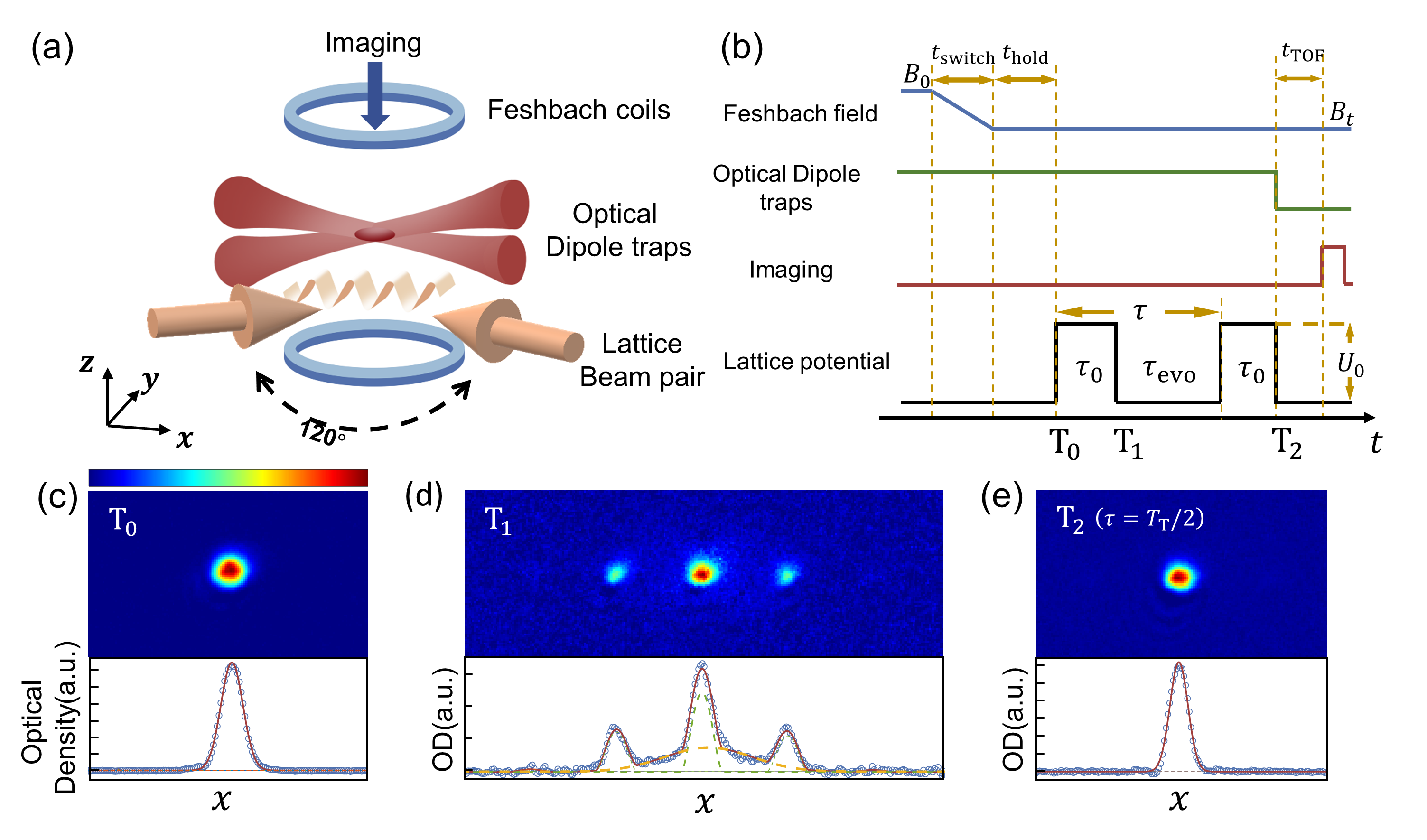
Fig.1(a) shows the schematic of the experimental set-up. The mBECs are confined in a trapping potential formed by a pair of far-red-detuned lasers in a vertical plane with a to each other. A pair of hollow electric coils produce the Feshbach Resonance magnetic field. The combined trapping frequencies are Hz, where -axis refers to the horizontal direction of the plane trapping beams located, the other horizontal direction, and the vertical direction. We use two beams of lasers, mutually separated by , to form a one-dimensional lattice potential in the horizontal direction, where is the lattice potential depth, the lattice spatial period. The lattice laser beams are focused to beam waists of . The beams are large compared to the size of the mBEC, and hence the lattice potential depth is approximately uniform across the cloud. The two lattice laser beams are derived from the same laser source, intensity controlled by an acousto-optic modulator (AOM), and split by a polarizing beam splitter to about 50:50, on-off controlled by two other AOMs synchronously. The characteristic lattice energy is , where and is the mass of a lithium molecule ().
The experimental time sequence is presented in Fig.1(b). After the completion of evaporation cooling, the Feshbach magnetic field is adiabatically () ramped from to within and kept for an additional duration of ms to stabilize. The lattice potential is then pulsed on twice with a variable evolution interval between. The Talbot interference time is defined by the sum of the evolution time and the duration of the first pulse . The optical dipole traps remain unchanged throughout the experiment, so a well-defined geometry and interaction energy are maintained during the scattering and interference process. After the second pulse, detection is performed by absorption imaging with ms TOF (time-of-flight). Fig. 1(c) depicts the absorption image after ms TOF before the first pulse () as mBEC. And Fig. 1(d) depict the ms TOF absorption imaging results taken after the first pulse (), showing the momentum distribution of particles after Kaptiza-Dirac(KD) scattering, which refers to two-photon scattering processes when particles move through a latticeGupta et al. (2001). The ms TOF image after the second pulse () with an interference time of is shown in Fig. 1(e).
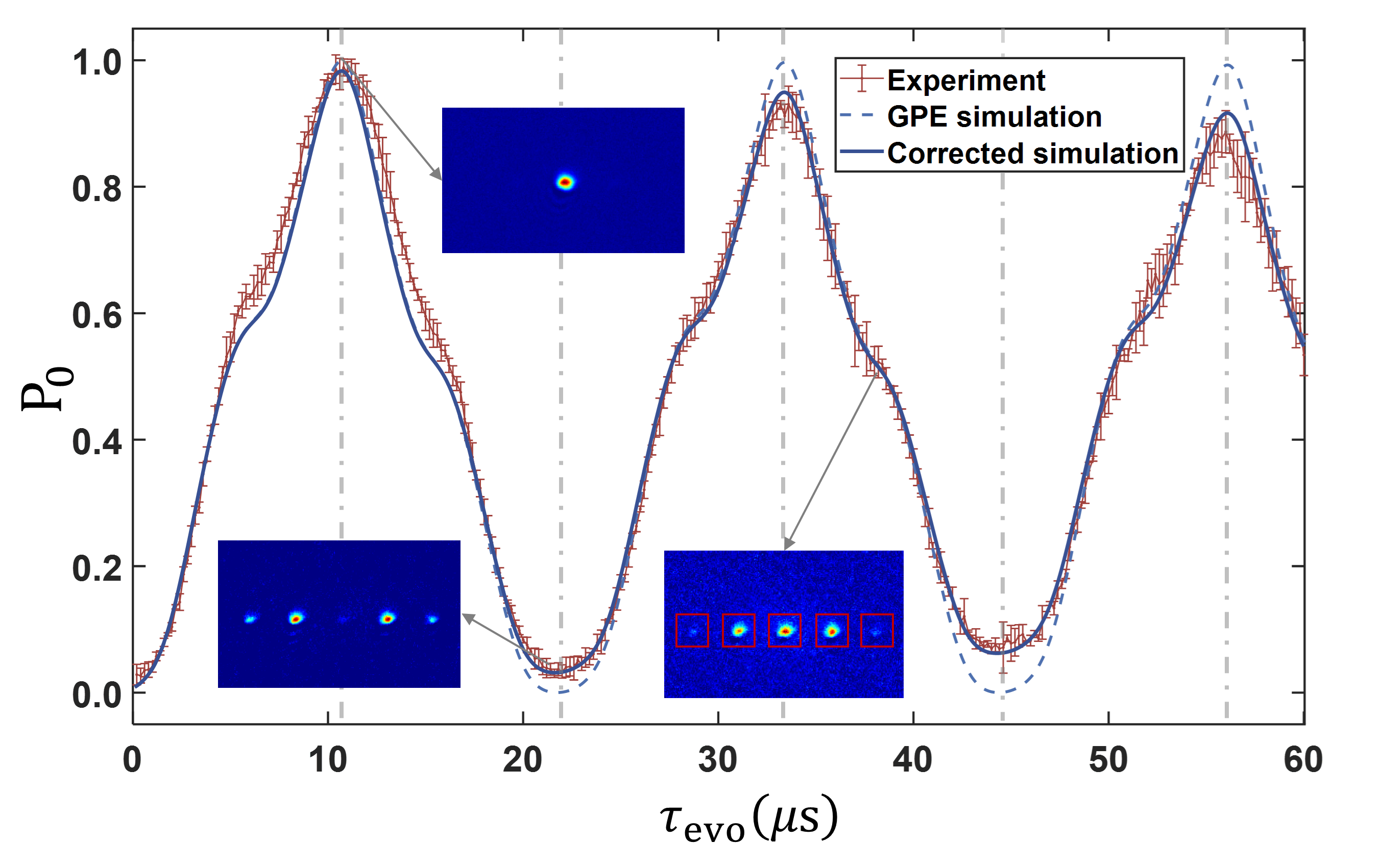
In the experiment, the lattice depth of the pulses, which is calibrated by KD scattering, is set to and the duration of both pulses is . The pulse time is short enough to keep within Raman-Nath regime Raman and Nagendra Nathe (1935) so that the particles remain approximately stationary during the lattice pulse and the interference process. In Fig. 2, the relative population as a function of the varied interval for is shown by the red dots, with changed every 0.2 up to . , in which is the particle number of modes, the total number of particles.
Here, we introduce Method 1 for obtaining Talbot signals (also the traditional one). and are obtained by integrating the number of particles in square regions near each momentum peak, as indicated by the red box in the inset. The side length of boxes is , equivalent to the range of for each momentum mode.
The Talbot time in our system is , while the theoretical value is . The two essentially stay the same, with the slight deviation attributed to a minute discrepancy in the angle of the lattice beams. The positions of multiples are indicated by gray dotted lines in Fig. 2. When there is no significant momentum broadening in the initial state or considerable interaction, will become maximal close to at odd multiples of the half Talbot time , minimal nearly at even multiples of , just as the theoretical simulation result shows (blue dashed line). However, in the case of strong interactions, the decay of the phase correlations cannot be ignored and is reflected in an exponential decay. We apply an exponential correction to the simulation result and find it aligns well with the experimental data.
III Theoretical analysis
To further understand the experiment, we conduct a theoretical analysis of the temporal Talbot interferometer under various interactions. The simulations employ a mean-field approach based on the Gross-Pitaevskii equation (GPE),
| (1) |
where is the mass of a molecule , is the combined trapping frequency, is the lattice potential and the effective interaction constant. In our system, the dynamics in the elongated direction are more relevant, while the transverse directions can be integrated out, leading to an effective 1D description with the 1D interaction parameter, . The is the Thomas-Fermi radius along the radial directions of the 3D mBEC and is calculated with the radial combined trapping frequencies (, ) which are calibrated at a set of scattering lengths.
We implement simulations of the Talbot interferometer with different interaction strength (scattering length ), different optical lattice pulses (lattice depth and pulse duration ), and different characteristic lattice energy . The simulation results under the same conditions as the experiment are presented in Fig. 2 and 4 for comparison, while the others are presented in Appendix. B to show the overall trend. It demonstrates that the effect of interaction on Talbot interference can be approximately determined by the values of and .
When is small, the signal curve changes quite little compared to the situation without interaction. For larger , the whole curve compresses towards , and the peaks exhibit a negative temporal shift as well as an amplitude decay. From an analytical perspective, the interaction term in (1) can be approximately treated as a shallow lattice term with a position-dependent amplitude. It induces an extra phase in the free evolution stage like an ordinary optical lattice, resulting in a positive correction on . Therefore, will decrease and cause a negative temporal shift on peaks. Meanwhile, a higher proportion of high-momentum modes is produced, strengthening the collision and decoherence among particles to make a signal damping. Both of these effects are caused by interactions during the evolution stage, rather than the lattice pulse stage.
Besides, as increases, a greater number of higher-order momentum modes emerge, accompanied by the appearance of sub-maximal peaks in the time domain, other than the principal maxima of the Talbot signal. The phenomenon is commonly referred to as the fractional Talbot effect, and there are some different behaviors under strong interactions.
IV Talbot signal damping under different interactions
To experimentally delineate the effect of interaction on the damping of temporal Talbot signals, we evaluate the decay rates for varying interaction strengths modulated via Feshbach resonance. The scattering lengths in experiment are designated as , , , . In our experiment, there is a notable reduction in particle count as decreases. To eliminate this disturbance, we utilize as the standard measure of interaction strength.
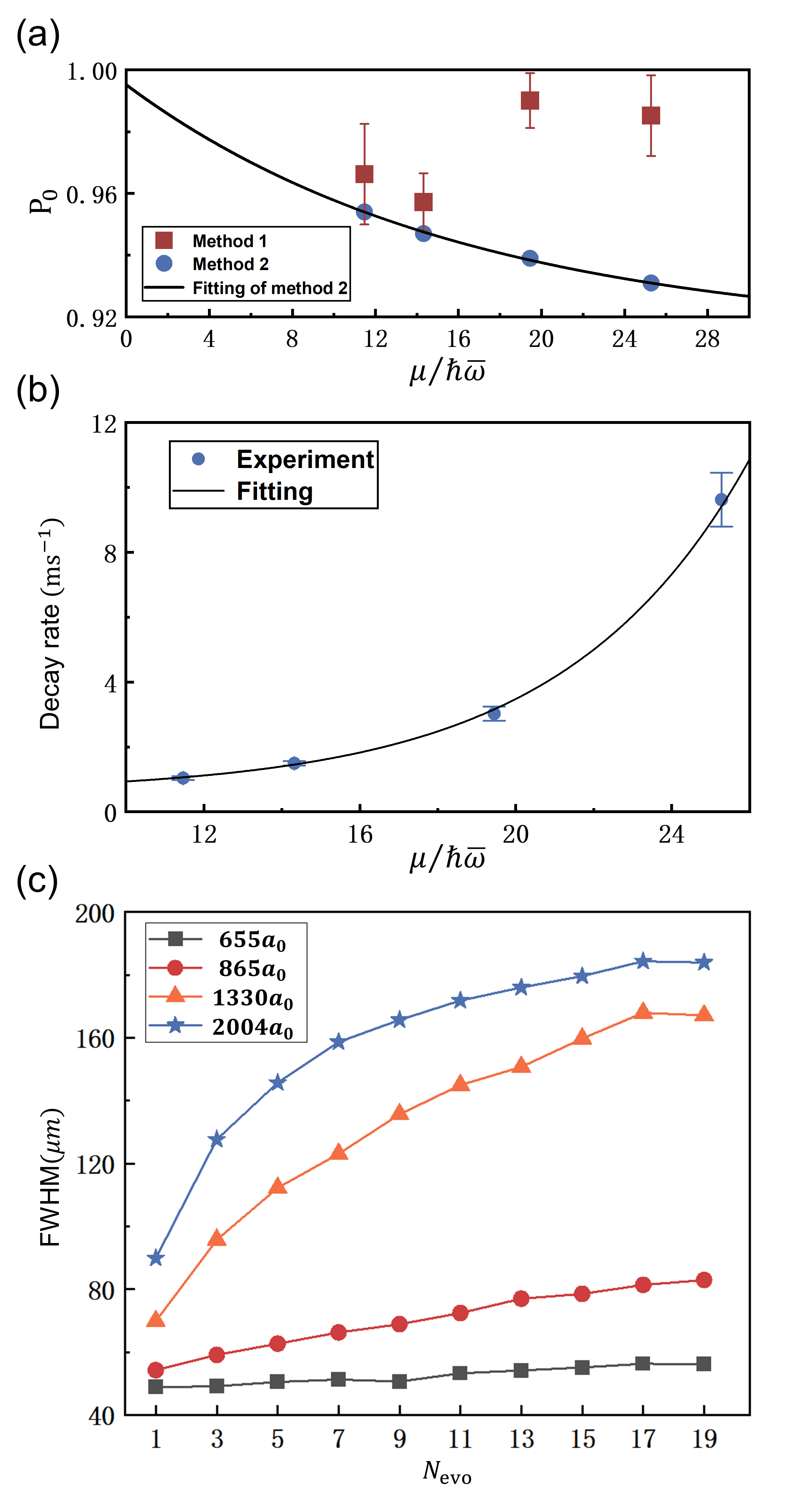
Initially, we employed Method 1 to acquire the signals. At , the first peak of showed no significant difference under varying interactions (red dots in Fig. 3(a)). We find that the damping effect does not increase monotonically with interaction strength, it diminishes after reaching a peak rather (refer to Appendix C for details). Analysis of the raw data reveals that strong interactions generate numerous thermal particles near the momentum mode, originating from collisions both during the interference phase and when different momentum components segregate during the TOF stage. These particles cause distortions in the Talbot signals and likely do not contribute to the oscillatory interference process. This influence becomes more pronounced when .
Adopting the method from Ref. Liang et al. (2022), we introduce Method 2 to refine the extraction of Talbot signals. A bi-modal fit is used to separate the condensed and non-condensed fractions, with the latter being excluded from the analysis of the Talbot signal (Fig. 1(d) bottom panel).
The signals from Method 2 at , represented by blue dots in Fig. 3(a), correspond to the averaged fitted results from 25 datasets. Contrary to the results from Method 1, a significant reduction in the amplitude of the first revival correlated with increased interaction strength is noted, implying that interactions induce damping during the pulse, initial evolution, and TOF stages. However, the effect is minor as remains above . Furthermore, the fitting of these points yields in the absence of interaction. Applying this method, we chart the decay across the first 10 revivals for four distinct interaction strengths to derive decay rates linearly (Appendix C). The absolute values of the slopes are considered as the decay rates, and represented by blue dots in Fig. 3(b). Upon fitting an exponential curve, we notice a significant increase in signal damping as the interaction strength increases. This indicates a significant impact of interaction on the evolution stage.
Despite its utility, Method 2 has some limitations. The bi-mode fit’s accuracy is questionable for peaks with few particles, and variations in fitting parameters can significantly alter the outcomes. Lastly, for interactions below , the fitting results are comparable with Method 1, except for the absence of error bars for individual data points.
For a more tangible perspective of interaction-induced damping, we plot the variation in the full width at half maximum (FWHM) of the molecular clusters in Fig. 3(c). For demonstration, the timeline has been simplified to , in which represents the actual Talbot time under various interactions. An augmented FWHM suggests a wider momentum distribution and reduced coherence. The FWHM escalates with higher interaction strengths, notably surpassing () when at . Correspondingly, values indicate an almost complete absence of condensed particles at zero momentum, signifying the interferometer’s breakdown.
V The interaction-induced Talbot period shift
To investigate the shift of the Talbot period due to varying interaction strengths, we conduct experiments within a fixed region, specifically around . This region is chosen because it accentuates the period shift while maintaining a relatively small decay of the signal. The selected time range is approximately one times . Then the experimental data are fitted with a no-interaction theoretical curve. The fitting process is guided by several parameters, which include the time scaling factor , signal oscillation amplitude , signal offset , and decay constant . The fitting expression is as follows:
| (2) | ||||
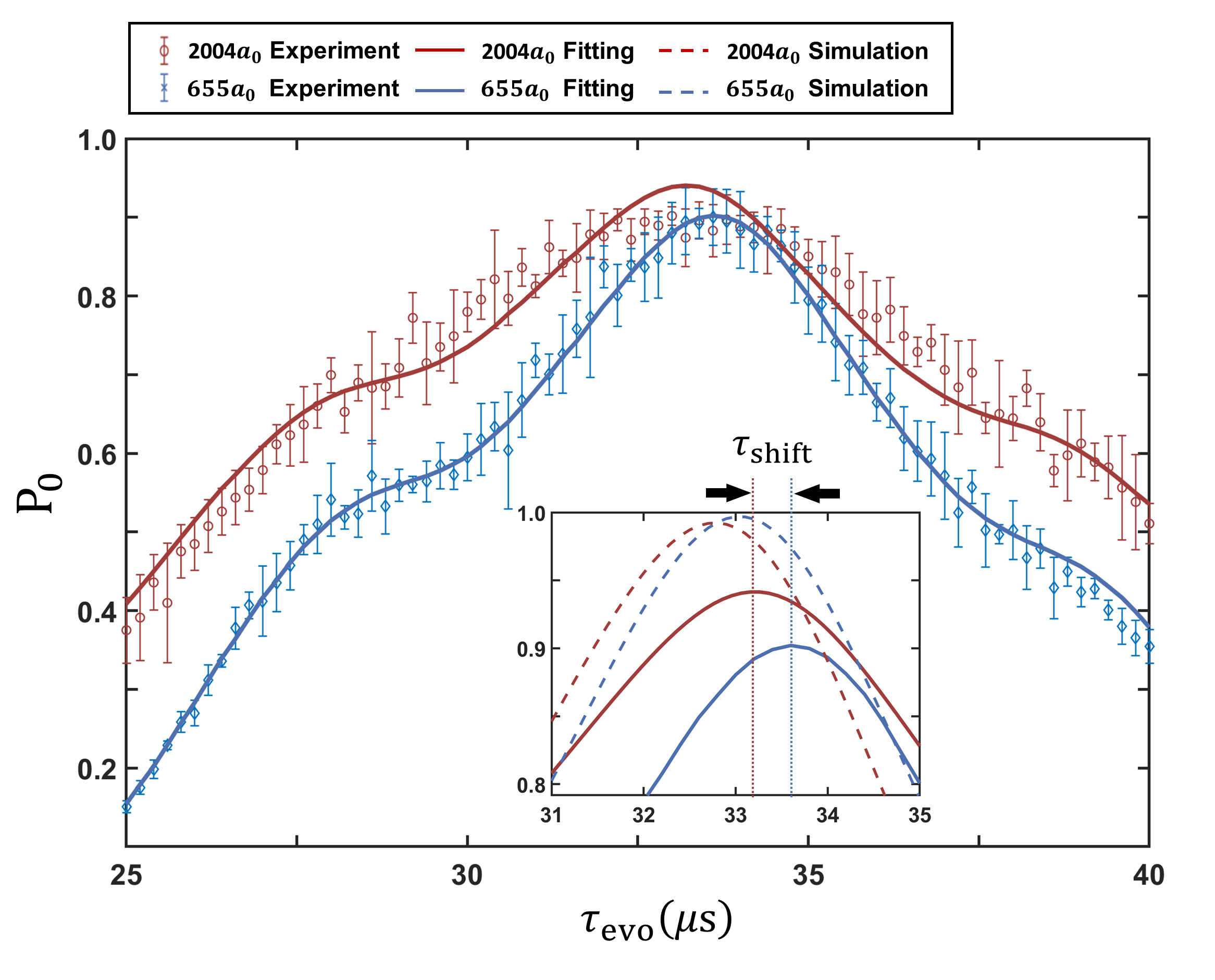
in which , , . The experimental results and corresponding fitting curves for interaction strengths of and are depicted in Fig. 4. We select the result with the smallest error after iterations of the fitting. Within the measured domain, the fitting curves are in good agreement with the experimental data points. A detailed view of the two curves around their respective maxima is presented in the inset, and the results of theoretical simulations are shown by the blue and red dashed lines. Table 1 presents the simulated and experimental values of aligned with the peaks under different interaction intensities.
TABLE I. The temporal shift of under different interactions. () Simulation () Experiment () 655 11.47 33.043 (0) 33.626 (0) 865 14.32 32.990 (-0.053) 33.527 (-0.099) 1330 19.45 32.904 (-0.139) 33.394 (-0.232) 2004 25.28 32.777 (-0.266) 33.082 (-0.544)
The parentheses indicate the under various interactions compared to those obtained under . The experimental and simulated results exhibit similar trends, with the values of also being relatively close. This change in , as described in Sec. III, originates from the interaction’s impact on or of optical lattices like an extra lattice.
Due to the limitations of the step size adjustment in the interference duration and the measurement errors near the maximum value, in experiments, it is only possible to qualitatively picture that increasing the interaction will shorten the Talbot time and cause a temporal peak shift. For quantitative measurements, as described in Sec. B, the accuracy can be enhanced by applying a pair of small-angle lattice beams with smaller .
VI Fractional Talbot effect
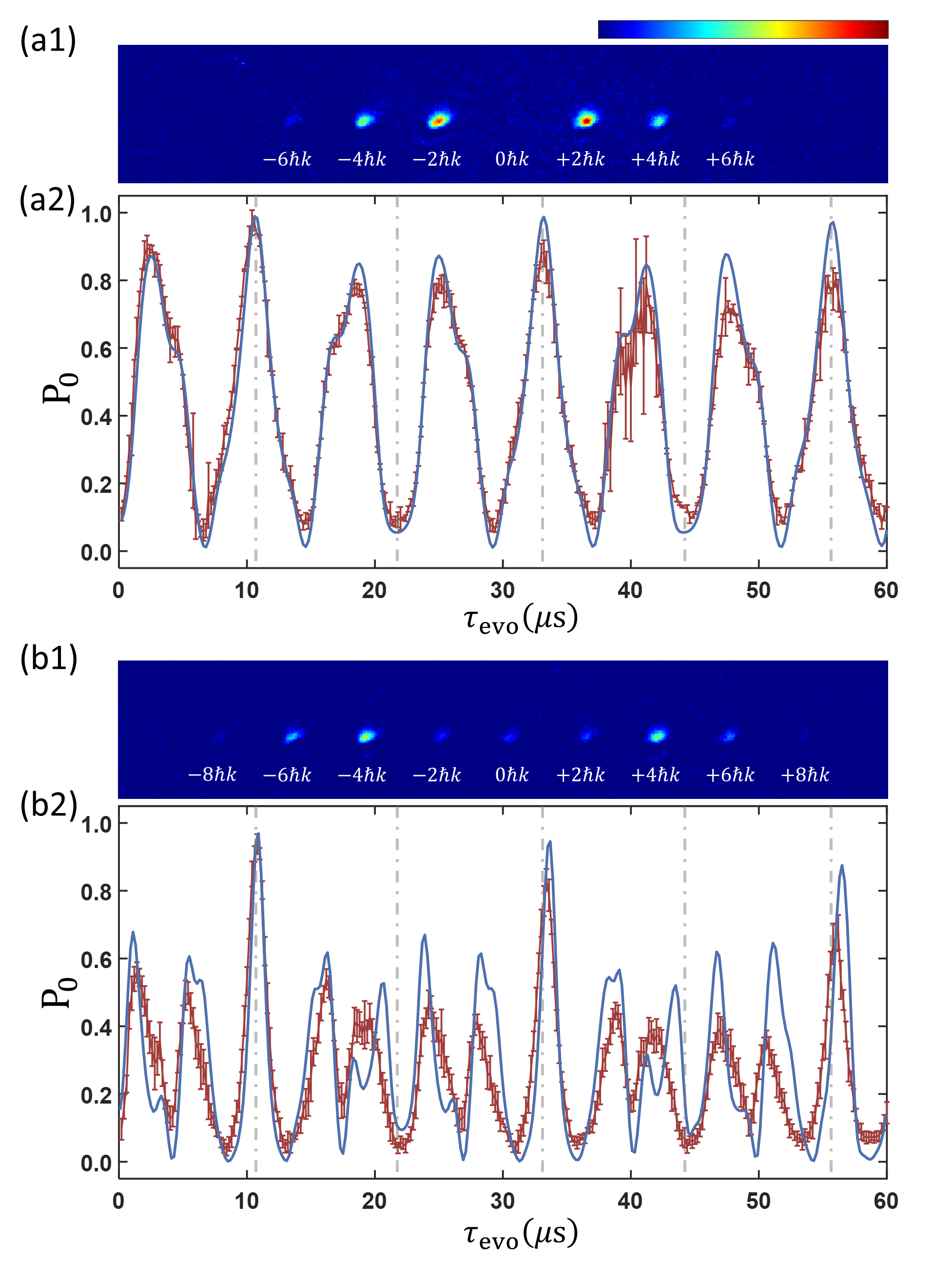
Considering the fractional Talbot interferometer Deng et al. (1999); Ullah et al. (2012) with higher-order momentum modes, collisions between particles with different momenta will become more intense during the interference process. To check the effectiveness under strong interactions, we modify the energy imparted to the particles by altering the initial and final pulses. We present the observation at different trap depths () and fixed pulse duration under the interaction strength of ( Gauss). The trap depth reaches values of and , giving a initial states () of Fig. 5(a1) and (b1). For a trap depth of , the peak of only appears when the evolution time equals to odd multiple of the half Talbot period. However, as illustrated in Fig. 5(a2), for a trap depth of , in addition to the maximum at odd multiples of , there are two sub-maxima appearing between two adjacent peaks, symmetrically distributed on both sides of the maximum peak. When the optical lattice depth is increased to , even more sub-maxima emerge, as illustrated in Fig. 5(b2). This observation is also confirmed by numerical simulations, showing the same results. The theoretical curves are marked by solid blue lines and the experimental data are marked by solid orange dots with error bars, in both Fig. 5(a2)(b2).
By comparing the initial states at different lattice depths, it can be observed that when the depths are respectively, the dominant momentum in the initial state is , , and , while the number of maxima appearing in each Talbot period is 1, 3, and 5. Thus we can conclude that this fractional Talbot effect is caused by the interference among higher-order momentum modes. Furthermore, for initial states dominated by , there will be maxima in each Talbot period. This conclusion is also supported by the results of GPE simulations.
The influence of interactions on the fractional Talbot interferometer can be observed through a comparison of experimental and theoretical curves. In addition to the previously mentioned decay, there are also changes in the shape of certain peaks. As for the signal decay, the changes in peak values at odd multiples of are not significantly different from those at low lattice depths. However, the decay of other sub-maxima is much faster, because the sub-maxima are mainly generated by higher-order momentum interference, and the dephasing caused by collisions between higher-order momentum modes is more pronounced as the interaction strength increases compared to lower-order momentum modes. The changes in peak shape arise from the slight modifications of the lattice depth due to interactions, which result in deviations between the experimental and theoretical initial states. Overall, the behavior of the fractional Talbot interferometer under strong interactions does not exhibit significant differences compared to the regular case.
VII Conclusion
In this study, we explore the effects of interaction on the Talbot signal’s damping and temporal shift in a one-dimensional optical lattice. Our findings indicate that interactions minimally influence the Talbot signal during the pulse sequence. Conversely, intensified interactions in the evolution stage accelerate the damping of the signal markedly. This is also reflected by the widening response in the half-width at half-maximum of the momentum modes. Additionally, interactions induce a slight drift in the Talbot time , resulting in an earlier peak occurrence. However, within the experimentally acceptable interaction range, this shift in Talbot time is practically inconsequential.
Across a wide range of interactions, the Talbot interferometer remains highly effective over a certain evolutionary timescale, inclusive of fractional Talbot interference scenarios. Under the modification of theoretical quantification, it can be utilized for lattice parameter calibration, momentum filtering, and coherence measurement in strongly interacting systems.
This work provides insight into the interplay between interaction and the coherence properties of a temporal Talbot interferometer in optical lattices, paving the way for research into quantum interference in strongly interacting systems.
Acknowledgements
The authors thank Wenlan Chen and Xiaopeng Li for helpful suggestions in building this setup. This work is supported by the National Natural Science Foundation of China (Grants No. 92365208, No.11934002, and No. 11920101004), National Key Research and Development Program of China (Grants No. 2021YFA0718300 and No. 2021YFA1400900); C.L. is supported by the Austrian Science Fund (FWF) through the ESPRIT grant 10.55776/ESP310 (EAPQuP).
Appendix A Experimental Apparatus
The experimental setup, as illustrated in Fig. 6, consists of an ultrahigh vacuum system comprising an atomic vapor oven, a Zeeman slower, and a science chamber. The vacuum pressure is maintained at an extremely low level of approximately in the oven section and a few in the experimental chambers, thanks to the presence of two titanium sublimation pumps and two ion getter pumps (/). Laser cooling is employed in three sequential steps: the magneto-optical trap (MOT), compressed magneto-optical trap (C-MOT), and gray molasses. The MOT collects lithium atoms, which have been laser cooled and collected from an oven through a Zeeman slower, at the experimental chamber using the line optical transition (). The MOT comprises cooling and repump lights that excite atoms from the and states, respectively, and typically captures around atoms at a temperature of approximately . The cooling and repumping beams are combined into the same optical fiber, which then generates three pairs of laser beams with a retro-reflection configuration. By ramping the laser frequency close to resonance and decreasing the optical intensity in the C-MOT, the temperature is further reduced to approximately , while maintaining around atoms. The loading of atoms into the MOT takes around seconds, and the C-MOT lasts for about ms. In our experiment, the cooling and repumping light for the gray molasses has a blue detuning of approximately from the line transition (), where the natural linewidth of the excited state is MHz. The laser beams for the gray molasses overlap with those of the MOT, facilitating optical alignment. The stage of gray molasses lasts for after switching off the magnetic field of the C-MOT, resulting in a reduction of the atomic temperature to , approximately one order of magnitude smaller.
The creation of a Bose-Einstein condensate (BEC) necessitates the application of various experimental techniques, as well as the provision of an ultrahigh vacuum environment and stable laser light for atom trapping and imaging. For , the creation of homogeneous magnetic fields to form bosonic molecules that can be condensed is an additional requirement. After transferring the atoms to the optical dipole trap (ODT), the quadrupole magnetic field of the MOT is switched off, and a pair of Helmholtz coils provides homogeneous Feshbach magnetic fields.

To achieve degenerate Fermi gases, we load cold atoms into an ODT for evaporative cooling. The ODT light is generated by a single-mode ytterbium-doped IPG fiber laser (YLR---LP-WC). The ODT light is turned on ms before the end of the MOT. By extinguishing the repumping light of the gray molasses earlier than the cooling light, the atoms are pumped to the states, which are the lowest two magnetic sublevels and . The configuration of the ODT is shown in Fig. 1(a), with two laser beams focused and intersecting in the science chamber at an angle of . The waist radius of the laser beam is . To avoid optical interference, two acousto-optical modulators (AOMs) are used to control the laser beams at frequencies of MHz and MHz, respectively. Evaporation cooling is then performed by decreasing the optical power of the dipole trap. The evaporation process is carried out under a magnetic field offset of Gauss, where the s-wave scattering length is infinitely large, resulting in strong interaction between the spin states and rapid thermalization. The ODT light is initially turned on with a power of W for each beam and kept on for approximately to reach equilibrium. The laser power is then ramped down through a two-stage exponential attenuation scanning process with a period of approximately . The percentage of laser power is monitored by a photodetector. In the first stages, the laser power is controlled by an external voltage, while in the final stages, a PI locking circuit is introduced to stabilize the optical intensity. As the laser power decreases, the atomic temperature also decreases. When the laser power is further ramped down to approximately , the Fermi gas becomes degenerate, with , where is the atomic temperature and is the Fermi temperature of the non-interacting Fermi gas.
Appendix B Calculation of Interacting Talbot Interferometers
To understand the effect of interaction in Talbot interference, we implemented (i) simulation at different scattering length with same optical lattice pulses (, ) and (ii) simulation at scattering length with same optical lattice pulses (, ) but different characteristic lattice energies.
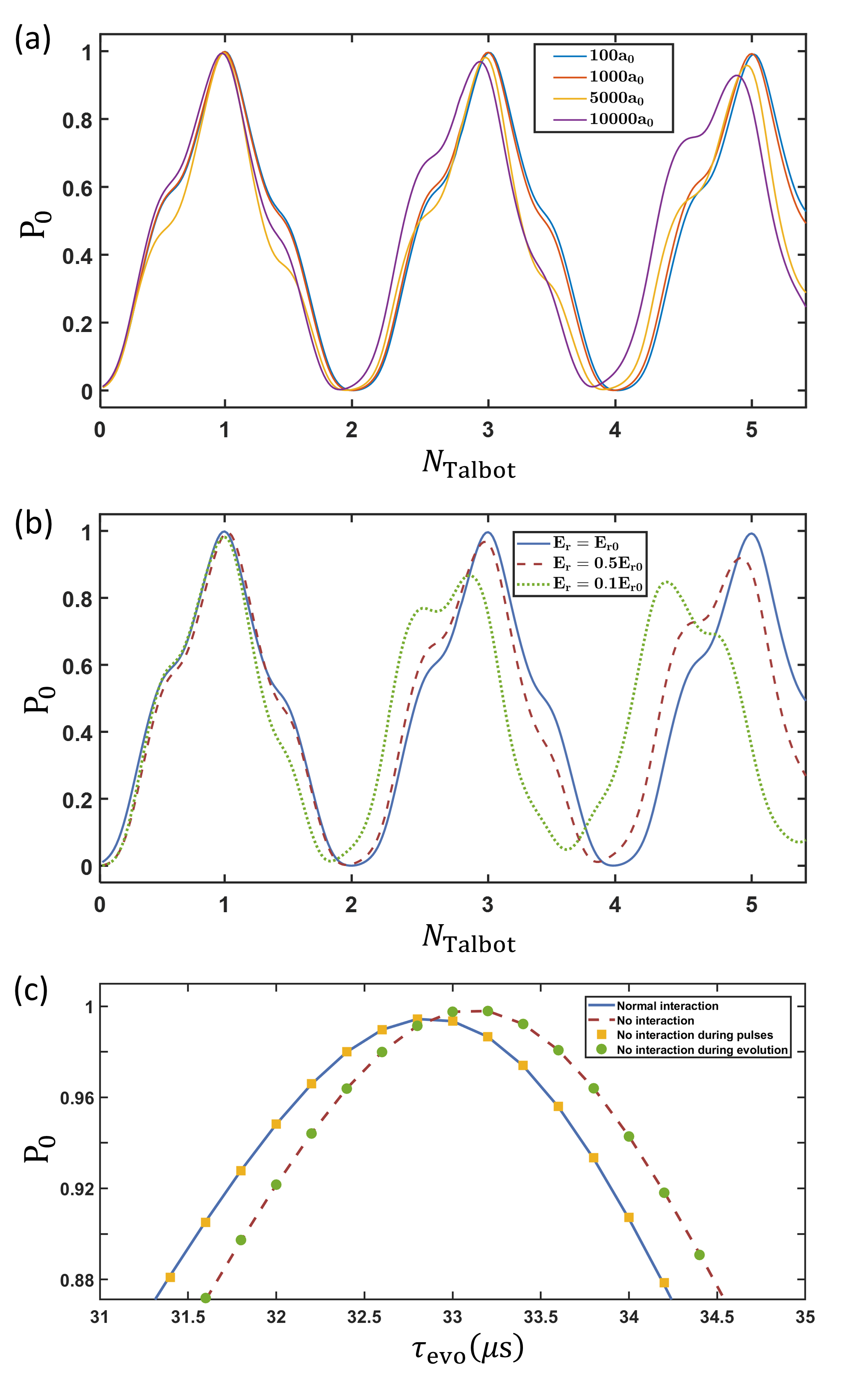
Fig. 7 (a) shows the results of (i), the Talbot effect with different interaction strengths. We observe increasing negative shifts of the peak in height and position with increasing scattering length. With a larger scattering length, the effect of interaction becomes significant so that the profile of the curve has slightly changed. Fig. 7 (b) shows the results of (ii), Talbot effect with the same interaction strength and optical lattice pulses for small characteristic lattice energy (larger lattice spatial depth ). With smaller values of , the Talbot effect shows similar changes in interaction as illustrated in Fig. 7(a), while the Talbot effect with no interaction remains unaffected. It is easy to understand because the decrease of equals the increase in interaction.
To distinguish the effect of interaction during the pulse stage and free evolution stage, we perform simulations by tuning interactions during these two stages separately. As demonstrated in Fig. 7(c), when the pulse stage is devoid of interaction, the results are indistinguishable from those where interactions are present throughout the entire interference process. Conversely, when the evolution stage lacks interactions, the results align with those obtained in the absence of any interactions during the entire sequence. It indicates that the influence of interaction focuses more on the free evolution stage. It is predictable because the lattice trap depth is too large for the interaction and the duration is too short for the free evolution time.
Appendix C Decay Sequences
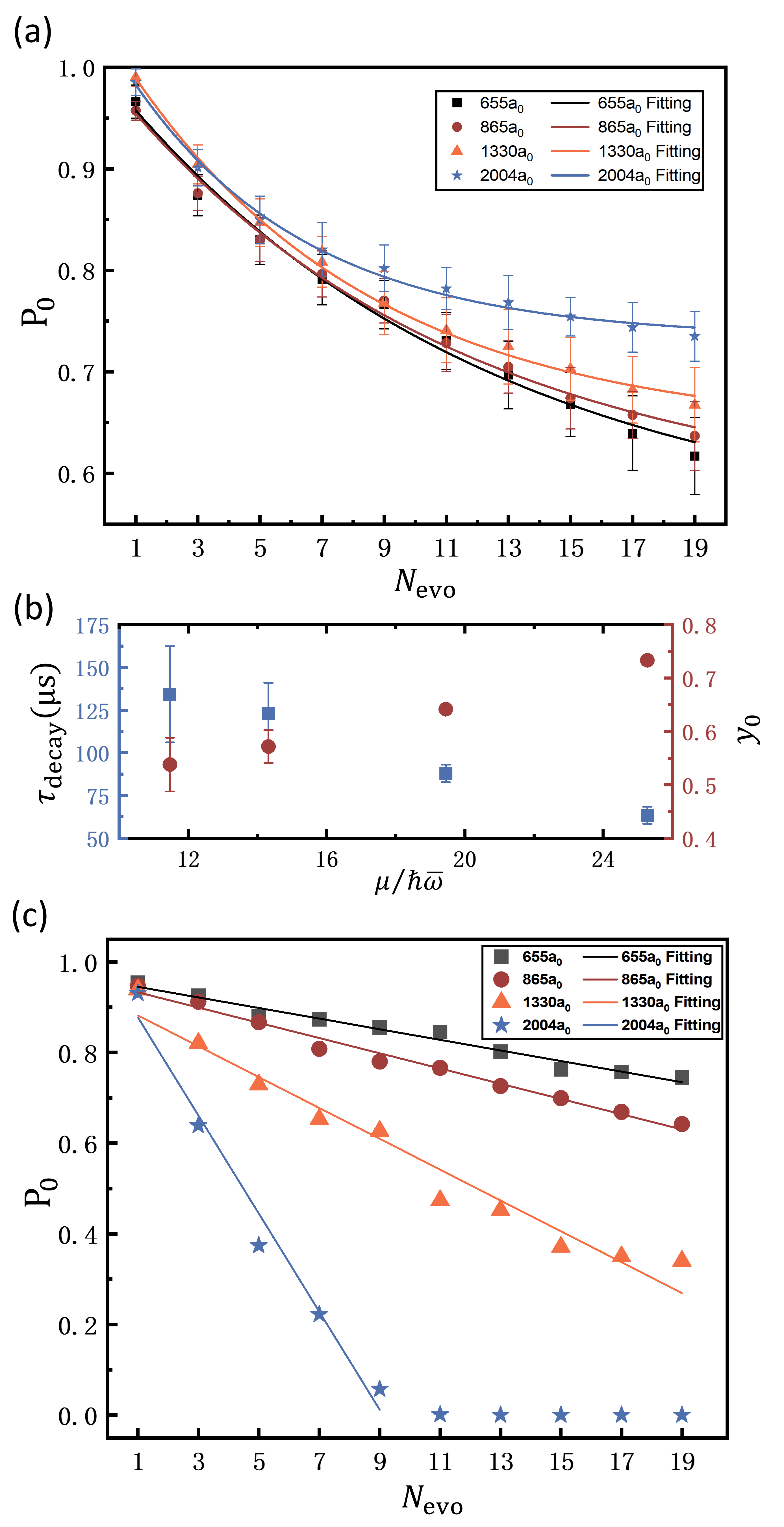
In Sec. IV, due to the disturbance caused by thermal particles near region in the Talbot signals obtained by the traditional method (Method 1) under strong interactions, we introduce Method 2 as the basis for judging signal damping. As shown in Fig. 8(a), the Talbot signal damping obtained through Method 1 under different interactions shows no significant relevance with interaction strengths. Even in the case of the highest interaction strength (), the decay curve appears the smoothest.
However, although the changes in signal damping observed are not intuitive, we can still obtain the effects of interactions from their fitting parameters. Considering the most common exponential fitting: , we extracted and under different interactions and presented them in Fig. 8(b). increases with higher interaction strengths, indicating that the interaction promotes the signal damping to approach a higher , which is in good agreement with our judgment of the influence of thermal particles generated during the interference period. Meanwhile, higher interaction strengths bring smaller , showing a shorter decay characteristic time scale, which agrees well with the decay constants obtained through Method 2. In summary, the experimental results obtained through Method 1 and Method 2 can both confirm the theoretical prediction that interaction leads to faster Talbot signal damping.
The decay curves obtained with Method 2 under different interactions are shown in Fig. 8(c). When we only include condensate parts in the calculation of the Talbot signal, the contrast of signal damping under different interactions is much better than the signal obtained from Method 1. When the interaction strength is below , the signal damping is very slow, even slower than the results obtained from Method 1. When the interaction strength is above , the decay significantly accelerates, and at , the proportion of condensate in the mode is almost zero. This is because the width of the thermal particle component remains almost constant, contributing to both the mode and the other higher modes (, ) regardless of the interaction. When the interaction strength is relatively weak, the optical density of the thermal particles is relatively small, and the contribution to the mode is smaller (in proportion) compared to the other higher modes, thus reducing the signal statistically. On the contrary, when the interaction strength is strong. Method 2 eliminates this disturbance and can therefore obtain a clearer Talbot signal variation curve. As for why the signal attenuation shows good linearity, further research is needed.
References
- Talbot (1836) H. F. Talbot, Philos. Mag 9 (1836).
- Lohmann and Silva (1971) A. Lohmann and D. Silva, Optics Communications 2, 413 (1971), ISSN 0030-4018, URL https://www.sciencedirect.com/science/article/pii/0030401871900551.
- Keren and Kafri (1985) E. Keren and O. Kafri, J. Opt. Soc. Am. A 2, 111 (1985), URL https://opg.optica.org/josaa/abstract.cfm?URI=josaa-2-2-111.
- Momose et al. (2003) A. Momose, S. Kawamoto, I. Koyama, Y. Hamaishi, K. Takai, and Y. Suzuki, Japanese Journal of Applied Physics 42, L866 (2003), URL https://dx.doi.org/10.1143/JJAP.42.L866.
- Momose et al. (2006) A. Momose, W. Yashiro, Y. Takeda, Y. Suzuki, and T. Hattori, Japanese Journal of Applied Physics 45, 5254 (2006), URL https://dx.doi.org/10.1143/JJAP.45.5254.
- Iwanow et al. (2005) R. Iwanow, D. May-Arrioja, D. Christodoulides, G. Stegeman, Y. Min, and W. Sohler, in 2005 Quantum Electronics and Laser Science Conference (2005), vol. 2, pp. 717–719 Vol. 2.
- Chen et al. (2015) Z. Chen, Y. Zhang, and M. Xiao, Optics express 23 11, 14724 (2015), URL https://api.semanticscholar.org/CorpusID:37359704.
- Dennis et al. (2007) M. R. Dennis, N. I. Zheludev, and F. J. G. de Abajo, Optics express 15 15, 9692 (2007), URL https://api.semanticscholar.org/CorpusID:12700622.
- Li et al. (2011) L. Li, Y. Fu, H. Wu, L. Zheng, H. Zhang, Z. Lu, Q. Sun, and W. Yu, Optics express 19 20, 19365 (2011), URL https://api.semanticscholar.org/CorpusID:207319740.
- Rayleigh (1881) L. Rayleigh, The London, Edinburgh, and Dublin Philosophical Magazine and Journal of Science 11, 196 (1881), eprint https://doi.org/10.1080/14786448108626995, URL https://doi.org/10.1080/14786448108626995.
- Zhang et al. (2010) Y. Zhang, J. Wen, S. N. Zhu, and M. Xiao, Phys. Rev. Lett. 104, 183901 (2010), URL https://link.aps.org/doi/10.1103/PhysRevLett.104.183901.
- Wen et al. (2013) J. Wen, Y. Zhang, and M. Xiao, Adv. Opt. Photon. 5, 83 (2013), URL https://opg.optica.org/aop/abstract.cfm?URI=aop-5-1-83.
- Deng et al. (1999) L. Deng, E. W. Hagley, J. Denschlag, J. E. Simsarian, M. Edwards, C. W. Clark, K. Helmerson, S. L. Rolston, and W. D. Phillips, Phys. Rev. Lett. 83, 5407 (1999), URL https://link.aps.org/doi/10.1103/PhysRevLett.83.5407.
- Mark et al. (2011) M. J. Mark, E. Haller, J. G. Danzl, K. Lauber, M. Gustavsson, and H.-C. Nägerl, New Journal of Physics 13, 085008 (2011), URL https://dx.doi.org/10.1088/1367-2630/13/8/085008.
- Yue et al. (2013) X. Yue, Y. Zhai, Z. Wang, H. Xiong, X. Chen, and X. Zhou, Phys. Rev. A 88, 013603 (2013), URL https://link.aps.org/doi/10.1103/PhysRevA.88.013603.
- Schäfer et al. (2020) F. Schäfer, T. Fukuhara, S. Sugawa, Y. Takasu, and Y. Takahashi, Nature Reviews Physics 2, 411 (2020), ISSN 2522-5820, URL https://doi.org/10.1038/s42254-020-0195-3.
- Jin et al. (2021) S. Jin, W. Zhang, X. Guo, X. Chen, X. Zhou, and X. Li, Phys. Rev. Lett. 126, 035301 (2021), URL https://link.aps.org/doi/10.1103/PhysRevLett.126.035301.
- Bloch et al. (2012) I. Bloch, J. Dalibard, and S. Nascimbène, Nature Physics 8, 267 (2012), ISSN 1745-2481, URL https://doi.org/10.1038/nphys2259.
- Niu et al. (2018) L. Niu, S. Jin, X. Chen, X. Li, and X. Zhou, Phys. Rev. Lett. 121, 265301 (2018), URL https://link.aps.org/doi/10.1103/PhysRevLett.121.265301.
- Yu et al. (2023) Z. Yu, J. Tian, P. Peng, D. Mao, X. Chen, and X. Zhou, Phys. Rev. A 107, 023303 (2023), URL https://link.aps.org/doi/10.1103/PhysRevA.107.023303.
- Weitenberg et al. (2011) C. Weitenberg, S. Kuhr, K. Mølmer, and J. F. Sherson, Phys. Rev. A 84, 032322 (2011), URL https://link.aps.org/doi/10.1103/PhysRevA.84.032322.
- Shui et al. (2021) H. Shui, S. Jin, Z. Li, F. Wei, X. Chen, X. Li, and X. Zhou, Phys. Rev. A 104, L060601 (2021), URL https://link.aps.org/doi/10.1103/PhysRevA.104.L060601.
- Guo et al. (2022) X. Guo, Z. Yu, F. Wei, S. Jin, X. Chen, X. Li, X. Zhang, and X. Zhou, Science Bulletin 67, 2291 (2022), ISSN 2095-9273, URL https://www.sciencedirect.com/science/article/pii/S2095927322004881.
- Dong et al. (2021) X. Dong, S. Jin, H. Shui, P. Peng, and X. Zhou, Chinese Physics B 30, 014210 (2021), URL https://dx.doi.org/10.1088/1674-1056/abcf33.
- Grond et al. (2010) J. Grond, U. Hohenester, I. Mazets, and J. Schmiedmayer, New Journal of Physics 12, 065036 (2010), URL https://dx.doi.org/10.1088/1367-2630/12/6/065036.
- Bloch (2005) I. Bloch, Journal of Physics B: Atomic, Molecular and Optical Physics 38, S629 (2005), URL https://dx.doi.org/10.1088/0953-4075/38/9/013.
- Hu et al. (2018) D. Hu, L. Niu, S. Jin, X. Chen, G. Dong, J. Schmiedmayer, and X. Zhou, Communications Physics 1, 29 (2018), ISSN 2399-3650, URL https://doi.org/10.1038/s42005-018-0030-7.
- Xiong et al. (2013) W. Xiong, X. Zhou, X. Yue, X. Chen, B. Wu, and H. Xiong, Laser Physics Letters 10, 125502 (2013), URL https://dx.doi.org/10.1088/1612-2011/10/12/125502.
- Gerbier et al. (2008) F. Gerbier, S. Trotzky, S. Fölling, U. Schnorrberger, J. D. Thompson, A. Widera, I. Bloch, L. Pollet, M. Troyer, B. Capogrosso-Sansone, et al., Phys. Rev. Lett. 101, 155303 (2008), URL https://link.aps.org/doi/10.1103/PhysRevLett.101.155303.
- Hofferberth et al. (2008) S. Hofferberth, I. Lesanovsky, T. Schumm, A. Imambekov, V. Gritsev, E. Demler, and J. Schmiedmayer, Nature Physics 4, 489 (2008), ISSN 1745-2481, URL https://doi.org/10.1038/nphys941.
- Dimopoulos et al. (2008) S. Dimopoulos, P. W. Graham, J. M. Hogan, and M. A. Kasevich, Phys. Rev. D 78, 042003 (2008), URL https://link.aps.org/doi/10.1103/PhysRevD.78.042003.
- Jannin et al. (2015) R. Jannin, P. Cladé, and S. Guellati-Khélifa, Phys. Rev. A 92, 013616 (2015), URL https://link.aps.org/doi/10.1103/PhysRevA.92.013616.
- Santra et al. (2017) B. Santra, C. Baals, R. Labouvie, A. B. Bhattacherjee, A. Pelster, and H. Ott, Nature Communications 8, 15601 (2017), ISSN 2041-1723, URL https://doi.org/10.1038/ncomms15601.
- Höllmer et al. (2019) P. Höllmer, J.-S. Bernier, C. Kollath, C. Baals, B. Santra, and H. Ott, Phys. Rev. A 100, 063613 (2019), URL https://link.aps.org/doi/10.1103/PhysRevA.100.063613.
- Chin et al. (2010) C. Chin, R. Grimm, P. Julienne, and E. Tiesinga, Rev. Mod. Phys. 82, 1225 (2010), URL https://link.aps.org/doi/10.1103/RevModPhys.82.1225.
- Ullah et al. (2012) A. Ullah, S. Ruddell, J. Currivan, and M. Hoogerland, The European Physical Journal D 66, 315 (2012), ISSN 1434-6079, URL https://doi.org/10.1140/epjd/e2012-30171-8.
- Bartenstein et al. (2005) M. Bartenstein, A. Altmeyer, S. Riedl, R. Geursen, S. Jochim, C. Chin, J. H. Denschlag, R. Grimm, A. Simoni, E. Tiesinga, et al., Phys. Rev. Lett. 94, 103201 (2005), URL https://link.aps.org/doi/10.1103/PhysRevLett.94.103201.
- Jochim et al. (2003) S. Jochim, M. Bartenstein, A. Altmeyer, G. Hendl, S. Riedl, C. Chin, J. H. Denschlag, and R. Grimm, Science 302, 2101 (2003), URL https://www.science.org/doi/abs/10.1126/science.1093280.
- Petrov et al. (2004) D. S. Petrov, C. Salomon, and G. V. Shlyapnikov, Phys. Rev. Lett. 93, 090404 (2004), URL https://link.aps.org/doi/10.1103/PhysRevLett.93.090404.
- Gupta et al. (2001) S. Gupta, A. E. Leanhardt, A. D. Cronin, and D. E. Pritchard, Comptes Rendus de l’Académie des Sciences - Series IV - Physics 2, 479 (2001), ISSN 1296-2147, URL https://www.sciencedirect.com/science/article/pii/S1296214701011799.
- Raman and Nagendra Nathe (1935) C. V. Raman and N. S. Nagendra Nathe, Proceedings of the Indian Academy of Sciences - Section A 2, 406 (1935), ISSN 0973-7685, URL https://doi.org/10.1007/BF03035840.
- Liang et al. (2022) Q. Liang, C. Li, S. Erne, P. Paranjape, R. Wu, and J. Schmiedmayer, SciPost Phys. 12, 154 (2022), URL https://scipost.org/10.21468/SciPostPhys.12.5.154.