[1]\fnmM. Daniela \surCuba
1]\orgdivSchool of Mathematics and Statistics, \orgnameUniversity of Glasgow, \countryUK 2]\orgnameBritish Geological Survey, \countryKeyworth, Nottingham, UK
A bivariate spatial extreme mixture model for unreplicated heavy metal soil contamination
Abstract
Geostatistical models for multivariate applications such as heavy metal soil contamination work under Gaussian assumptions and may result in underestimated extreme values and misleading risk assessments [23]. A more suitable framework to analyse extreme values is extreme value theory (EVT). However, EVT relies on replications in time, which are generally not available in geochemical datasets. Therefore, using EVT to map soil contamination requires adaptation to be used in the usual single-replicate data framework of soil surveys. We propose a bivariate spatial extreme mixture model to model the body and tail of contaminant pairs, where the tails are described using a stationary generalised Pareto distribution. We demonstrate the performance of our model using a simulation study and through modelling bivariate soil contamination in the Glasgow conurbation. Model results are given as maps of predicted marginal concentrations and probabilities of joint exceedance of soil guideline values. Marginal concentration maps show areas of elevated lead levels along the Clyde River and elevated levels of chromium around the south and southeast villages such as East Kilbride and Wishaw. The joint probability maps show higher probabilities of joint exceedance to the south and southeast of the city centre, following known legacy contamination regions in the Clyde River basin.
keywords:
Coregionalisation models, Extreme Value Theory, Extreme Mixture Models, Soil Contamination, Unreplicated Extremes1 Introduction
Heavy metal soil contamination is the above-baseline accumulation of heavy metals (HMs) in the soil [33, 32, 28]. The most common biological toxic HM elements are mercury (Hg), cadmium (Cd), lead (Pb), chromium (Cr), arsenic (As), zinc (Zn), copper (Cu), nickel (Ni), stannum (Sn, technical name for tin), and vanadium (V). While trace amounts of HMs are indispensable in the environment, acute and chronic exposure via direct contact, or through the digestive and respiratory tracts, pose a significant risk to public health [29].
The main pathways for excessive HM accumulation in urban and rural environments are often anthropogenic [14]. In urban areas, primary sources include industrial waste and residue, chemical manufacturing, sewage, atmospheric deposition, and combustion of fossil fuels [33, 19]. HM soil contamination is generally characterised by its wide spatial distribution, strong latency, irreversibility, and complex multivariate nature [32]. The remediation of contaminated soils is relatively slow compared to the remediation of contaminated water or air [19]. For this reason, understanding the extent and intensity of the contamination, particularly in urban and densely-populated areas, is essential to establish preventive public health measures and mitigate the impacts of soil HM contamination [14].
HM contamination is usually mapped using data from soil surveys [35], which use spatial sampling schemes, prioritising the spatial distribution as dictated by each contaminant’s properties and other environmental factors [17]. Concentration values are commonly modelled by performing a Box-Cox transformation (typically log transformation) followed by a Gaussian process regression model such as trans-gaussian kriging [8, 20, 22]. However, HM contamination distributions are known to be heavy-tailed, a property which persists even after transformation and is not captured using the Gaussian framework [23, 24]. As a result, Gaussian models underestimate extreme values at the tails, which may result in an underestimation of the risk of public exposure to high levels of HM contamination.
Extreme Value Theory (EVT) is the natural statistical framework for the analysis of extreme values. Recent years have seen a growing interest in EVT for environmental applications such as climate science or hydrology [34], motivating theoretical extensions to model extremes in spatial and multivariate settings. Classical EVT distributions define extreme values as the maximum value inside a block (block-maxima) or values exceeding a given threshold (threshold exceedances). For the definition of the block-maxima approach, let be a set of iid continuous random variables and represent the maxima. The extremal types theorem [6] states that if there exist sequences and such that the normalisation of as converges to a non-degenerate function as , then belongs to the family of generalised extreme value distributions (GEV) [10, 11, 27]. Threshold exceedances, also known as the peak-over-threshold approach (POT), represent an alternative to the block-maxima approach and are defined as observations of that exceed a given threshold , i.e., . If the conditions for the limiting characterisation of given above hold, threshold exceedances converge to the generalised Pareto distribution (GPD) when , with distribution function characterised by a scale and a shape parameter, and given by
| (1) |
An essential requirement for EVT is that of replications in time. In environmental applications, temporal replicates are generally available for phenomena with a temporal dimension. However, soil surveys are generally unreplicated, meaning replications in time are rarely available and preventing the use of EVT for applications such as mapping HM contamination. Additionally, the multivariate nature of HM contamination shows the presence of concomitant extremes, which may be of special interest for public health planning due to the complexity posed by the risks associated with multiple contaminants. It is clear then that a suitable spatial statistical modelling of HM contamination requires the use of multivariate spatial models that do not underestimate the marginal extreme behaviours, are able to capture extremal dependence between contaminants across space, and can handle unreplicated data.
We propose to fill the gap between classical EVT based on replications and unreplicated multivariate spatial settings by using a continuous mixture of non-extreme and extreme distributions. Our methodology is proposed for the bivariate case where two contaminants are modelled simultaneously, accounting for the extremal dependence between variables through a coregionalisation framework. We assume the distribution of each contaminant can be decomposed into two components, representing the body and the tail of the distribution. The body of the distribution is composed of a combination of natural pedogenic processes and diffuse background contamination and represents the majority of the observations [1]. The tail contains the extreme concentrations from contaminating anthropogenic or natural processes [24]. Each component is modelled using suitable distributions for extreme and non-extreme concentrations and woven together using a continuous mixture model representation. In principle, the body and tail processes of two contaminants can be differently affected by the same spatial factors, so we allow the mixture components to share spatial effects across variables inside a coregionalisation framework. Inference on the model is performed using the integrated nested Laplace approximation (INLA; [31]), which allows Bayesian inference for the class of latent Gaussian models (LGMs) and can be fitted in R using the package R-INLA. Coregionalisation models are straightforward to fit with R-INLA [18]; however, mixture models lack the LGM representation needed for INLA, so we adapt a conditional approach following Gómez-Rubio and Rue [13]. We assess our model using a simulation study and present a case study using data from the Geochemical Baseline Survey of the Environment (G-BASE) in the Glasgow Conurbation, where we show that our model correctly captures the tail behaviour of a bivariate geochemical dataset. An important byproduct of our modelling approach are risk maps showing probabilities of two contaminants jointly exceeding their respective safety values as defined by the soil guideline values (SGV; Cole and Jeffries 5).
The remainder of this manuscript proceeds as follows. Section 2 provides an overview of the necessary statistical background. The coregionalised mixture model we propose is presented in Section 3. In Section 4, we detail the simulation study performed to assess the performance of our proposed model and present the results. Section 5 presents the results of the model fitted to chromium and lead as contaminant pairs in the Glasgow Conurbation, showing marginal concentrations and probability plots of joint exceedance of SGVs. Finally, Section 6 provides a discussion. Supporting plots and tables are given in the Appendix.
2 Statistical background
2.1 Latent Gaussian models
Latent Gaussian models (LGM) represent a wide subclass of structured additive regression models [9]. Let represent the response vector with an assumed distribution in the exponential family of distributions with density function where denotes a vector of hyperparameters. Using a link function , can be linked to covariates through linear predictors
where is an intercept, is a vector of coefficients representing the linear effects of on , and are unknown non-linear functions of covariates . A latent Gaussian model (LGM) arises in the case where a Gaussian prior is assumed for the latent field . A Bayesian hierarchical structure can be easily defined for the LGM, as
| (2) | ||||
where are hyperparameters from the likelihood () and the latent prior ().
The aim of inference for LGM is the estimation of , the latent field, for which we need the marginal posteriors and . In its Bayesian hierarchical representation, it is possible to use Bayesian inference techniques such as MCMC to perform inference on LGMs. However, these techniques are often computationally unfeasible for large datasets [31]. The integrated nested Laplace approximations (INLA) framework was proposed by Rue et al [31] as a computationally efficient inference framework for LGMs. In the original formulation of INLA, the linear predictors were included in an augmented latent field
However, this results in a singular covariance matrix of , requiring the addition of a Gaussian noise term in as
| (3) |
where , with a large but fixed [36]. This enhancement is no longer necessary in the new formulation of INLA. Here, the latent field is defined as before
with the Gaussian prior . The linear predictors are defined as
where is a sparse design matrix linking the linear predictors to the latent field [36].
The Gaussian approximation to is calculated from a second order expansion of the likelihood around the mode [36] resulting in
where represents a precision matrix. The univariate conditional posteriors follow naturally from the joint Gaussian approximation as
| (4) |
The marginal posterior can be obtained by integrating out of 4 by using points of integration, [36].
The marginal posteriors of the linear predictors were automatically calculated in the original INLA formulation of Rue et al [31]. However, the new formulation requires first calculating . The resulting posterior means of and , based on the Gaussian assumption of the conditional posterior, can be inaccurate [36]. A Variational Bayes correction to the means, proposed by van Niekerk and Rue [30], can improve the posterior means of the latent field. The corrected posterior inference fo is
where are the weights of the integration points when computing the marginal posterior of .
2.2 Mixture models
A mixture model is a convex, weighted combination of multiple distributions representing the different assumed underlying groups in the data. An observation is assumed to come from one of data generating processes, each with their own set of parameters [26], i.e.,
| (5) |
where is a set of parametric distributions (one for each latent group in the data), and are their associated weights with .
Unless we assume the mixture weights are known, mixture models do not have a latent Gaussian representation. Consequently, inference cannot be carried out in INLA without adjustment [12], as in the augmented data approach in Dempster et al [7]. This approach considers an auxiliary variable that assigns each observation to a group in the set . The mixture model can then be represented as
The distribution of can be stated as
resulting in the likelihood
where is the number of observations in group . When conditioning on , under the assumption that the groups are independent, the mixture model has a latent Gaussian representation and can be fitted with INLA using various possible approaches such as Gomez-Rubio [12] and Gómez-Rubio and Rue [13]. Gomez-Rubio [12] shows that the posterior marginal of the conditional mixture model can be represented as
The above requires the posterior distribution of , which can be estimated using the INLA within Monte Carlo Markov Chain (MCMC) approach in Gómez-Rubio and Rue [13]. The adjustment to produce the latent Gaussian representation requires conditioning on fixed parameters or hyperparameters of , denoted as . Denoting the non-fixed parameters by , the resulting posterior can be expressed as
where is a LGM suitable for INLA. Although it is possible to perform inference on using MCMC or importance sampling [2], we choose a fixed a priori value for due to computational limitations. The choice of is done using an extensive grid search of possible values and model-performance metrics to assess optimum values.
2.3 Coregionalisation framework
Multivariate response models with latent Gaussian characterisations can be fitted inside the coregionalisation framework [18]. The framework allows for a different likelihood function for each variable and models the dependence structure between variables by introducing shared components in the linear predictor. In the bivariate case, let and be two spatial variables for locations . Simple linear predictors for a coregionalisation model can be defined as
| (6) | ||||
where and are the linear predictors at of and , respectively, and are intercepts, and are spatial random effects [21], and is a weight for the shared spatial effect [18]. In essence, the linear predictors of and are dependent on a shared component, , which captures dependence between variables. While has a single spatial effects term, can have a second spatial effects term (), adding flexibility to the model. Inference on the model is easily performed in INLA [18], using two likelihoods. It can be extended beyond the bivariate case to include different likelihoods for each response variable, but the implementation is restricted due to the tradeoff between accuracy and computational costs. Additionally, the linear predictors can also contain linear and non-linear effects, as well as more shared components of different forms.
3 Proposed methodology and inference
Our bivariate spatial extreme mixture model for unreplicated data combines bivariate mixture models for an accurate representation of the body and tail of the distribution of each contaminant while a coregionalisation structure incorporates the spatial dependencies within a latent Gaussian model framework. Specifically, we construct two spatial mixture models with mixing components for variables and at locations . The components account for the body and tail observations of each variable. The spatial mixture models are defined as
| (7) |
where, for , is the density of the non-extreme observations in the body, is the density of the extremes in the tail, and is the mixing proportion or the probability that an observation belongs to the body of the distribution. From Section 2.3, the coregionalisation framework is defined through linear predictors with shared components. For our mixture models in (3), we carefully explored the inclusion of shared components on the bulks and tails to account for dependence at non-extreme and extreme values, respectively. Even though the shared components are flexible and can be tailored for each application, components should be linked only when necessary since increasing the number of shared components considerably increases computational costs. Our coregionalised mixture model shares spatial components only in the tails to account for extremal dependence, while the non-extreme components have shared dependence only through common covariates. The model can be expressed as
| (8) | ||||||
where for and are the corresponding linear predictors for and respectively, and are random spatial effects, are covariates, and are intercepts, and are coefficients corresponding to the covariates for the body and tail respectively, and is a scaling coefficient for the shared random spatial effect . Although different likelihoods can be assigned to each component (namely, , , and ), our specific application driven by the need to correctly characterise extreme and non-extreme HM concentrations, motivates the use of a Gaussian likelihood for the bodies and , and a generalised Pareto distribution (GPD) for the tails and . By using the GPD we are implicitly defining extreme observations as exceedances over suitably high thresholds and for and , respectively.
Inference for our model is based on the conditional latent Gaussian field framework proposed by Gómez-Rubio and Rue [13], where we replace the MCMC inference with a simple conditional approach based on conditioning parameters a priori, similar to the importance sampling approach to conditional mixture models by Berild et al [2]. As noted in Section 1, the GPD requires replicates over time. The implementation of the GPD likelihood in INLA links the linear predictor to a fixed -quantile of the distribution, specifically, with . This parametrisation implicitly assumes replicates at each location . Interestingly, this is not the case for the Gaussian likelihood, where latent Gaussian models can be fitted following the usual geostatistical design of single replicates over space. To circumvent the need for replications of tail values, we assume spatial stationarity of threshold exceedances and model the tail of each HM contaminant using a stationary GPD as in (1). Then, we transform the tail values to a common Gaussian scale using the probability integral transform. Finally, tail values in our bivariate spatial extreme mixture model are modelled using the alternative tail distribution density
| (9) |
where represents the extreme values constituting the tail of contaminant, is the standard normal distribution and is the GPD fitted to all exceedances of the threshold for variable . As per the transformation in (9), the two distributional components of the coregionalisation model are Gaussian and non-informative Gaussian priors are assigned to all components of the linear predictors. Pointwise predictions and their uncertainties can be obtained using posterior samples, with the necessary back-transformation for values belonging to the tail.
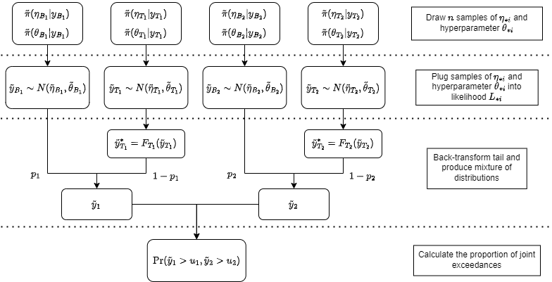
For risk assessment purposes, we also derive joint exceedance probability maps. Specifically, we compute , where and are sufficiently high threshold (following soil guideline values). These values are obtained by sampling from the posterior predictive distribution, which can be done using a multi-step Monte Carlo method summarised in Figure 1. It is first necessary to sample from the posteriors of the linear predictor and the hyperparameters. These samples are then used to obtain samples of the posterior predictive distribution of each component after a back-transformation of the tail distribution and mixing of the distributions according to the mixture proportions and as in (3). Finally, the joint exceedance probabilities are computed empirically. This process is repeated to obtain measures of uncertainty of the Monte Carlo procedure.
4 Simulation study
In this section, we show the construction and results of an extensive simulation study aimed at assessing the performance of the proposed bivariate spatial extreme mixture model for a single realisation mimicking HM soil contamination. A total of four scenarios were considered, set up to mimic behaviour observed in real geochemical datasets.
4.1 Data-generating process
The data were simulated directly from the model in (8) after the adjustment proposed in (9). We produced a total of simulations of observations over the region for two response variables, and . The random spatial effects are simulated as Gaussian Processes (GP) with Matern covariance function [25] defined as
where is the Euclidean distance between two observations, is the gamma function, is the modified Bessel function of the second kind, is the range of spatial dependence, and is the smoothness parameter. Parameter values for the proposed simulation scenarios are given in Table 1.
| Parameter | A | B |
|---|---|---|
| (0.75, 0.75) | (0.75, 0.75) | |
| (0.9, 0.9) | (0.9, 0.9) | |
| (1,0) | (1,0) | |
| (1,0) | (1,0) | |
| (0.1,0.25) | (0.1,0.25) | |
| (0.1,0.25) | (0.1,0.25) | |
| 0.25 | 0.9 | |
| (10, 15) | (10, 15) | |
| (1,1) | (1,1) | |
| (0.05, 0.25) | (0.5, 0.25) |
4.2 Classification
The model requires a priori classification of observations as belonging to the body or tail of the distribution. While the choice of mixture proportion also defines threshold , given that the proportion of observations exceeding threshold is the same as , setting all exceedances from as belonging to the tail results in an upper truncation for the body. As a result, we propose a classification based on the Metropolis-Hastings algorithm, which results in a soft boundary between body and tail. The classification is as follows
-
1.
For the body and tail distributions, and , respectively, estimate all parameters using maximum likelihood.
-
2.
For each observation in compute the density under and under as and respectively.
-
3.
Obtain the classification ratio .
-
4.
Draw a random sample from a uniform distribution .
-
5.
Assign the observation as belonging to the tail if .
-
6.
Repeat the process times for each observation and assign the membership that appears the most number of times in the samples.
4.3 Evaluation
Assessment is performed by quantifying the true parameter coverage probability (the probability that the true parameter value is in the confidence interval), as well as the parameter estimation error using root mean squared error (RMSE) computed as
Generally, a small RMSE indicates a good model fit, given that the predicted parameter values are close to the true parameter values. The assessment of the categorisation of observations as body or tail, a form of pre-processing, is performed using standard categorisation evaluation techniques such as computing the accuracy, sensitivity, specificity, and precision.
4.4 Results
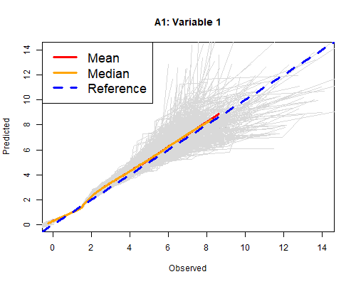
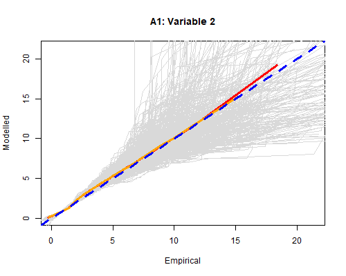
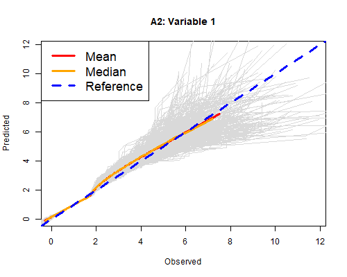
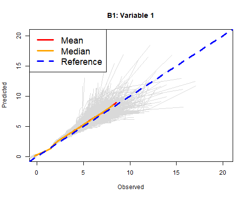
Figure 2 shows the Q-Q plots of the results for simulation A1. The figure shows that the model performs better for (variable 1), displaying smaller variability at higher values than (variable 2). However, both the median and the mean of the simulations for both variables accurately capture the true behaviour of the data for the body and tail of the distributions. Table 2 shows the coverage probability for the parameters of the linear predictor, and . We can see that they are well captured and have coverage probabilities greater than , with the exception of , which might account for abrupt behaviour around the transition between body and tail. Of the remaining parameters, only has lower coverage probabilities, indicating the fit is not as good in as in , as is expected given the asymmetric construction of the model.
| Parameter | True Val | Mean | Median | Sd | Coverage Pr | RMSE |
|---|---|---|---|---|---|---|
| 1.00 | 1.04 | 1.04 | 0.01 | 0.99 | 0.04 | |
| 0.00 | -0.22 | -0.23 | 0.05 | 0.38 | 0.23 | |
| 1.00 | 1.05 | 1.04 | 0.03 | 0.99 | 0.06 | |
| 0.00 | -0.24 | -0.23 | 0.07 | 0.88 | 0.25 | |
| 0.10 | 0.07 | 0.07 | 0.01 | 0.99 | 0.03 | |
| 0.25 | 0.18 | 0.18 | 0.01 | 0.99 | 0.07 | |
| 0.10 | 0.07 | 0.07 | 0.06 | 0.97 | 0.07 | |
| 0.25 | 0.18 | 0.18 | 0.04 | 0.98 | 0.09 | |
| 0.10 | 0.08 | 0.07 | 0.01 | 0.99 | 0.03 | |
| 0.25 | 0.19 | 0.19 | 0.02 | 0.99 | 0.06 | |
| 0.10 | 0.07 | 0.07 | 0.06 | 0.98 | 0.07 | |
| 0.25 | 0.18 | 0.18 | 0.05 | 0.98 | 0.08 | |
| 0.01 | 0.20 | 0.19 | 0.10 | 0.74 | 0.22 | |
| 0.01 | 0.14 | 0.13 | 0.06 | 0.96 | 0.15 | |
| 10.00 | 38.79 | 28.83 | 35.70 | 0.89 | 45.78 | |
| 15.00 | 129.62 | 90.98 | 172.25 | 0.80 | 172.48 | |
| 0.25 | 0.97 | 0.97 | 0.08 | 0.32 | 0.73 | |
| 1 | 1.004 | 0.99 | 0.14 | 0.92 | 0.14 | |
| 1 | 1.16 | 1.14 | 0.17 | 0.89 | 0.23 | |
| 0.05 | 0.06 | 0.06 | 0.11 | 0.93 | 0.11 | |
| 0.25 | 0.27 | 0.27 | 0.12 | 0.95 | 0.94 |
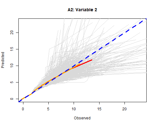
The results for A2 show a pattern similar to that of A1. The Q-Q plots in Figure 9 in the Appendix show a larger variability displayed in the tail of than in . Additionally, is slightly underestimated at extreme values. Table 3 in Appendix summarises the parameter estimates. Once again, the linear coefficients of are well captured by the model while is consistently overestimated, similar to A1.
The performance assessments of the classification of observations as body or tail for A1 and A2 are given in Table 4 in the Appendix. Carried out a priori with the method in Section 4.2, the classification of both is approximately of the observations begin classified correctly.
Scenario B had a larger value for the weight of the shared spatial component, , indicating stronger extremal dependence between variables. Figure 10 in the Appendix shows that for variable 1, the model performs as expected, similarly to results in A1 and A2. Variable 2 follows the pattern seen in A1 and A2, where variability is increased in the tail. However, in this scenario, the mean and median show a slight overestimation at the extremes. Table 5 in Appendix shows the model has good coverage probabilities for most parameters. The large standard deviation of the range parameters, and , show the model struggles to calculate the range of the spatial components, a possible explanation for the increased variability in the tails of the distribution.
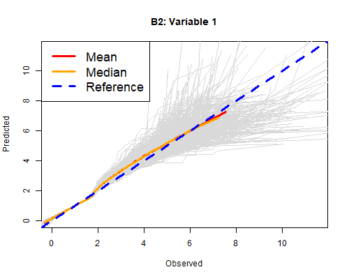
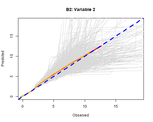
The results for B2 are shown in Figure 11 in the Appendix. The model performs similarly to B1, with the mean showing sensitivity to large values and a correct median for both variables. The summary of the estimated model parameters in Table 6 show that the model correctly estimates most parameters, with the exception of and , which experience an even bigger variability in estimation than previous scenarios. The coverage probability of the ranges, and seems to be lower for Variation 2, meaning the model struggles to accurately estimate the range when there are fewer extreme observations.
The classification of the observations for B1 and B2 (Table 7) is similar to scenario A. The relatively lower specificity values indicate a poorer categorisation of the tail observations than the body. Overall, the results indicate the model did not suffer a loss of power with a larger imbalance in classes.
5 Case Study: Heavy Metal Soil Contamination Glasgow Conurbation
The bivariate spatial mixture model was applied to the log-transformed concentrations of Cr and Pb in the Glasgow Conurbation using data from the Geochemical Baseline Survey of the Environment (G-BASE; see Johnson et al 15 for details). The results of the model are compared to a standard Gaussian model with no mixture where both contaminants are fitted independently.
5.1 Data Description
The British Geological Survey (BGS) performed the G-BASE survey from the 1960s to 2014 [15]. Initially commissioned for mineral exploration, it is a valuable tool for the systematic assessment of the geochemical background of the UK environment. The area of interest is the Glasgow Conurbation in the Clyde River Basin, west of Scotland, where the data consist of approximately topsoil (5-20cm deep) samples taken at approximately observations per in the urban areas and per in rural areas. Each sample was decomposed chemically using X-ray fluorescence and the concentration of each element in the sample in parts per million (ppm). Further details can be found in Johnson et al [15].
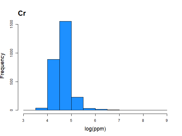
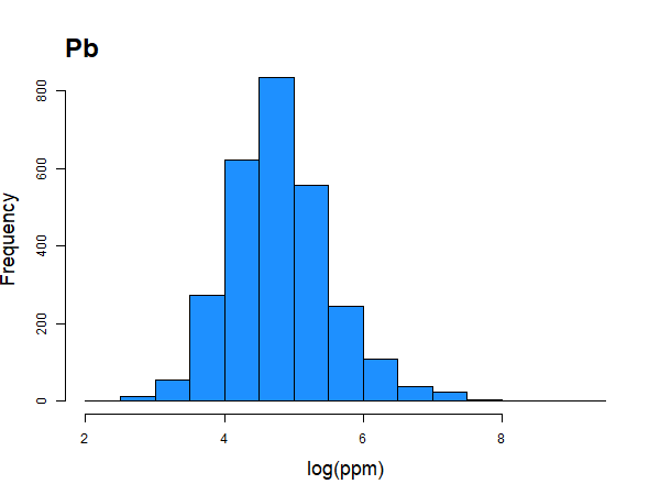
As a pre-processing step, the data are first transformed using a log transformation. Figure 3 shows histograms of the data post-transformation. Although the data appear approximately normal, kurtosis is 18.32 and 4.69 for Cr and Pb, respectively. The kurtosis shows that the tail of Cr is significantly heavier than that of a normal distribution, whereas Pb has a lighter tail that is just outside the expected values for a Gaussian distribution of the same sample size. This again highlights the need for an alternative approach to the usual Gaussian modelling that focuses on accurate estimation of the tails of the HM distribution.
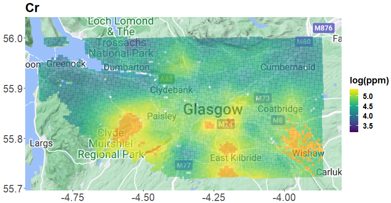
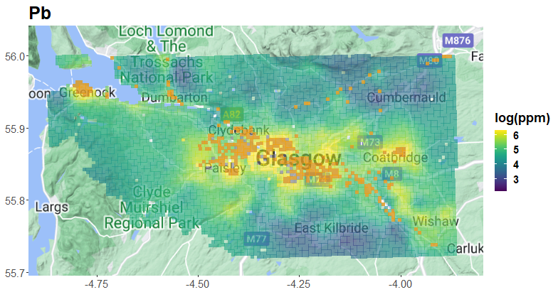
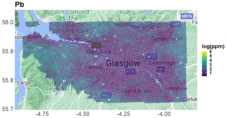
Maps of the concentrations of Cr and Pb can be seen in Figure 4. The top row shows the full range of concentrations of Cr and Pb after a log transformation, respectively. The bottom row maps display a continuous scale of observations up to the 95th quantile. The observations exceeding this threshold are in solid orange colour and the maximum value is shown in red. In this scale, the 95th quantile corresponds to log(ppm) for Cr and log(ppm) for Pb, while the maximum values are log(ppm) and log(ppm) for Cr and Pb respectively. The map shows an agglomeration of high values just south of the Clyde in central Glasgow, while other high values can also be found in Coatbridge, East Kilbride, and Wishaw to the south and southeast. To the southwest, high values are seen around Paisley and further south towards Clyde Muirshiel Reginal Park. High values for Pb are found near Greenock Port and Dumbarton, especially along the M74 and the A82 towards The Trossachs National Park and the port of Greenock.
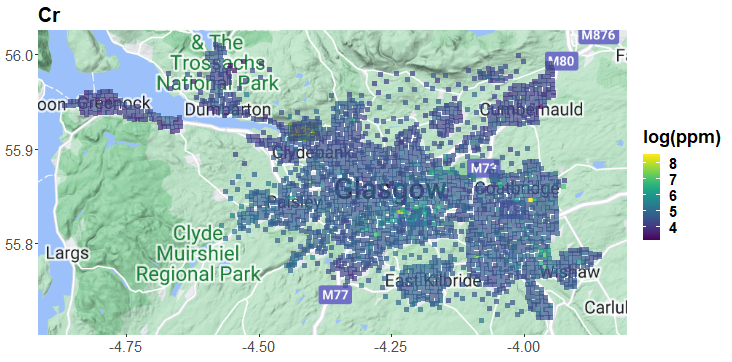
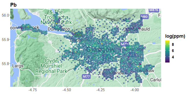
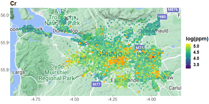
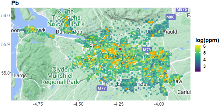
Soils Data BGS © NERC. Map data © 2023 Google.
Following Johnson et al [16], we obtained terrain and topography variables for model covariates such as elevation, slope, aspect, multiresolution index of valley bottom flatness (MRVBF), the complementary multiresolution index of the ridge top flatness (MRRTF), and topographic wetness index (TWI) from a digital elevation model (DEM) by the Ordinance Survey (OS) at a resolution of 1:50000. Processing of the data was done in R using RSAGA [3]. Variables providing proximal traffic information such as the type of nearest road, primary (A) or secondary (B), and distance to the nearest primary and secondary roads were obtained from the UK Department of Environment, Food, and Agricultural Affairs (DEFRA). The covariates were introduced in the linear predictor as linear fixed effects.
5.2 Results
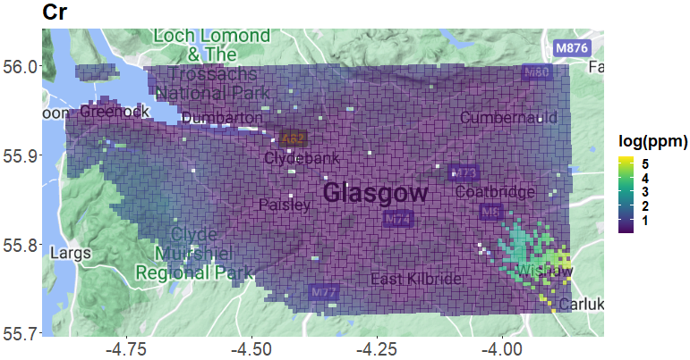
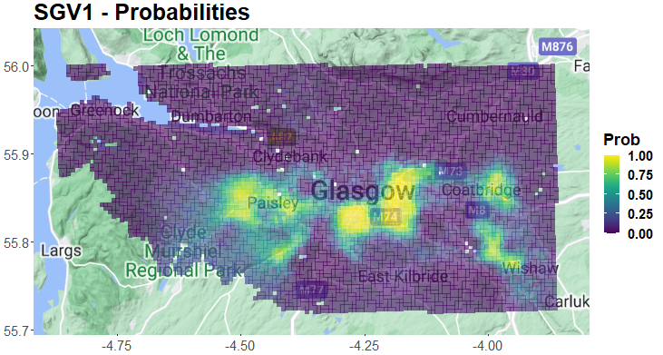
The a priori classification of observations as body or tail depends on the parameters and , corresponding to the mixture proportions of and respectively, which indicate the probability of an observation belonging to the body of the distribution. Unlike the simulation study, and are not known; therefore, an exhaustive search for appropriate values is performed using a grid of values from to in increments of , and the values for and that yield the best DIC and predictive RMSE values are selected. In the case of the Cr-Pb pair, the best model performance was given by and . A prediction using a spatial binomial model is made over a rectangular region representing the spatial extent of the observations in order to obtain the classification of prediction locations (Figure 5). The binomial model captures the pattern of extreme observations in Figure 4, where extreme concentrations of Cr are clustered south of the Clyde in Glasgow and Wishaw. The predictions for Pb also capture the true pattern, with extreme or tail observations found along the M74, the A82, and Coatbridge.
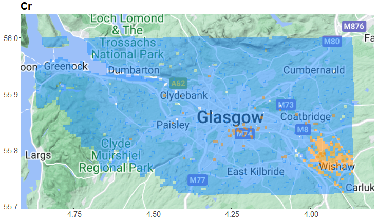
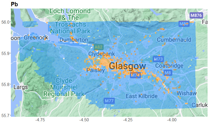
Soils Data BGS © NERC. Map data © 2023 Google.
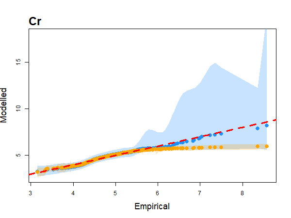
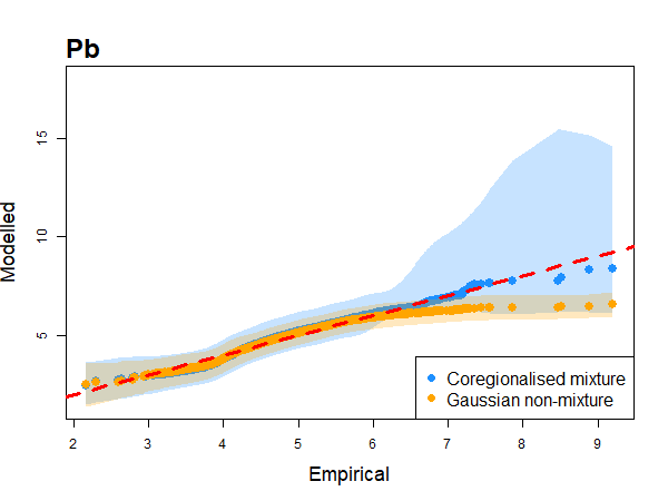
Our bivariate spatial extreme mixture model in (8) is fitted to the rectangular area representing the spatial extent of the observations to obtain a continuous prediction of the concentrations of Cr and Pb in the river basin. Model validation is performed using k-fold cross-validation, with where every fold removes of the observations and performs predictions on the removed locations. Figure 6 compares the cross-validation predictions of the coregionalised mixture model to a non-mixture Gaussian model fitted in INLA where both components are fitted independently of each other and provides the smoothed credible intervals. The larger width of the credible intervals of the coregionalised mixture model is expected due to the heavier tail of the GPD distribution compared to the Gaussian model. For Cr, we see the deviation is greater, which is understandable given the heavier tail of the Cr distribution as corroborated by its estimated kurtosis. On the other hand, the difference between models is less distinct for Pb and can be explained due to lower kurtosis. Overall, the coregionalised mixture model shows an improvement over the Gaussian model in capturing extreme values and modelling a heavy-tailed distributions.
The results given in Figure 7 provide maps of the model results as marginal concentrations. The figures show that Cr has new predicted areas of contamination in the Wishaw area to the southeast. The area between the city centre and East Kilbride to the south experiences higher concentrations too, which match the observed data. Other areas of raised predicted Cr concentrations are west of Paisley to the west of Glasgow, and Coatbrige to the east. Pb shows similar trends to those anticipated. The M74 road around the city centre and to the south through Wishaw are singled out as having especially high concentrations, as does the Port of Greenock and the A82 towards the Trossachs National Park. Additional predicted areas of contamination include the M80 near Falkirk to the southeast. Overall, higher concentrations can be found along more densely populated areas from Paisley to the west to Coatbridge in the east and around major A and M roads with heavy traffic.
Soils Data BGS © NERC. Map data © 2023 Google.
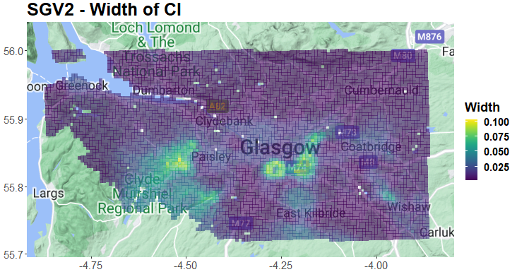
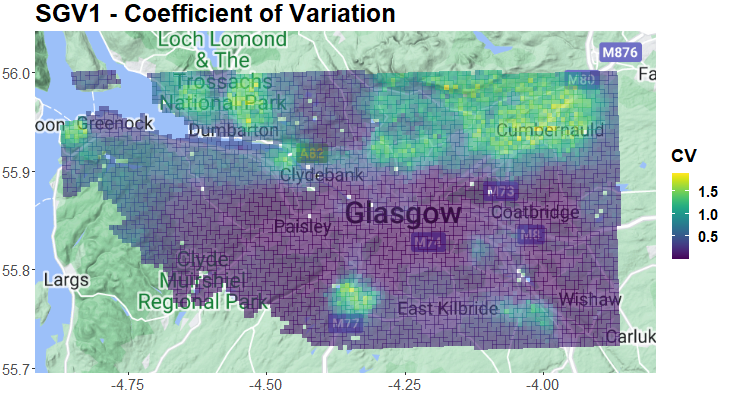
Assessing the risk posed by both contaminants simultaneously is possible using joint exceedance probability maps. The Environment Agency in the UK has published SGV for most HM elements [5], indicating what concentration thresholds are considered safe. In residential areas with no plants or food production (SGV1), Cr is recommended to stay under 130ppm, 4.87 in log(ppm), and Pb under 200ppm, 5.30 log(ppm). In residential areas with plant or food production (SGV2), the SGV is 200ppm for Cr and 310ppm for Pb, or 5.29 log(ppm) and 5.74 log(ppm) for Cr and Pb, respectively. Using the process described in Figure 1, we computed the probabilities of joint exceedance of SGV1 and SGV2 using samples from the posterior predictive distribution. The maps in Figure 8 show that Cr and Pb have high probabilities of exceeding SGV1 in the south, southeast, and east of the city of Glasgow. These areas are well-known for legacy contamination due to historical chromium ore processing and other chromium-producing industries [4]. The figures also show that the uncertainties given by the confidence intervals are small and do not affect interpretation. The coefficient of variation, defined as the ratio of the standard deviation to the mean, shows that areas of high probability exhibit small relative variation, whereas the areas of low probability, mainly to the north of the city, show larger variation in relation to the mean.
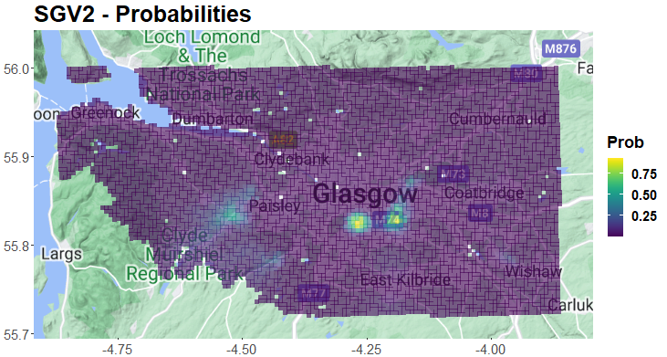
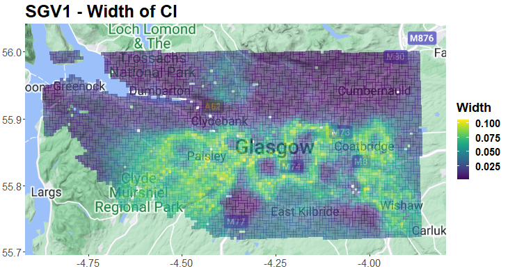
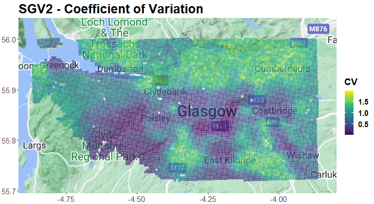
The maps for SGV2 show a similar result where there is only a high probability of both contaminants exceeding the threshold in two contamination hotspots in well-known areas to the south and southeast of the city centre. Additionally, there are higher probabilities to the southwest, near Paisley. Uncertainty maps show the two hotspots of contamination with high certainty, while contamination detected to the southwest is more uncertain. Areas of low probability, such as the north, show greater variability in relation to the mean, similar to SGV1.
Soils Data BGS © NERC. Map data © 2023 Google.
6 Conclusion and Discussion
Maps of geochemical concentrations are generally produced using geostatistical models under a Gaussian framework. Such models do not account for the various processes responsible for the spatial distribution of geochemical concentrations but rather model all observations as realisations of a single Gaussian process, resulting in an underestimation of extreme values and measures of risk . When more than one contaminant is present, classical geostatistical models not only under-estimate extreme concentrations, but also do not account for the extremal dependence between contaminants. We propose to partition the distribution of each contaminant into body and tail, representing non-extreme and extreme concentrations, and weaving them together inside a coregionalised mixture model framework. The body component, representing non-extreme observations linked to a combination of natural pedogenic processes and diffuse background contamination, is modelled using a Gaussian model common to geochemical applications. The tail, containing extreme observations related to contaminating anthropogenic or natural processes, is modelled using an adapted extreme value distribution. While EVT is an attractive framework to capture extremal behaviour, it requires replications at each location, which are not commonly available in geochemical datasets. For this reason, a transformation is applied to the tail under a stationary GPD, and later modelled under a Gaussian likelihood following the usual geostatistical setting of a single replication. Our proposed framework combines ideas from coregionalisation models, mixture models, spatial latent Gaussian models, and EVT to capture non-extremal concentrations as well as the extremal behaviour and dependence between two contaminants at high concentrations and produce a continuous map of concentrations.
We fit our model to Cr and Pb concentrations in the Glasgow Conurbation in the west of Scotland. The data was first transformed using a log transformation, and kurtosis provided evidence of the deviation of the tails from a Gaussian distribution. The results of the model show that there are areas of Cr contamination to the south and southwest of Glasgow, southwest of Paisley, to the south around East Kilbride, and to the east near Wishaw. Areas of high Pb concentrations are found around the Glasgow city centre and seem to be contained to areas around the Clyde River and the Port of Greenock. Marginal credible intervals are the widest for observations belonging to the tail, which is expected for extreme observations due to the limited sample size. The model shows that joint contamination has a high probability of exceeding SGV1 and SGV2 in the south and southeast of the city of Glasgow, areas known to be affected by legacy industrial HM contamination. A comparison with a classical Gaussian model shows that the joint modelling of two contaminants using the coregionalised mixture model is an improvement, particularly at the tail. Furthermore, the shared spatial random component models the factors affecting the extreme values of both contaminants while the weight of the shared spatial component, , models the dependence between both tail distributions. High values of can account for strong extremal dependence between components while indicates extremal independence.. For this application, we constrained the dependence structure to only account for extremal dependence through a shared spatial random effect. However, the framework is flexible and can be easily extended to capture dependence through other terms in both the body and tail or extended beyond the bivariate case. Future work can be developed to jointly model and in space and integrate this modelling with the coregionalised mixture model. A natural way to do this is through a hierarchical Bayesian model where inference is carried out using simulation-based approaches, such as MCMC.
Appendix
| Parameter | True Val | Median | Mean | Sd | Coverage.pr | RMSE |
|---|---|---|---|---|---|---|
| 1.00 | 1.02 | 1.02 | 0.01 | 0.99 | 0.03 | |
| 0.00 | -0.12 | -0.11 | 0.10 | 0.96 | 0.15 | |
| 1.00 | 1.03 | 1.02 | 0.01 | 0.99 | 0.03 | |
| 0.00 | -0.12 | -0.11 | 0.10 | 0.99 | 0.16 | |
| 0.10 | 0.09 | 0.09 | 0.01 | 0.99 | 0.01 | |
| 0.25 | 0.22 | 0.22 | 0.01 | 0.99 | 0.03 | |
| 0.10 | 0.04 | 0.04 | 0.10 | 0.97 | 0.12 | |
| 0.25 | 0.07 | 0.06 | 0.08 | 0.64 | 0.20 | |
| 0.10 | 0.09 | 0.09 | 0.01 | 0.99 | 0.01 | |
| 0.25 | 0.22 | 0.22 | 0.01 | 0.99 | 0.03 | |
| 0.10 | 0.04 | 0.04 | 0.11 | 0.94 | 0.12 | |
| 0.25 | 0.08 | 0.07 | 0.09 | 0.70 | 0.19 | |
| 0.01 | 0.33 | 0.25 | 0.23 | 0.60 | 0.40 | |
| 0.01 | 0.21 | 0.15 | 0.17 | 0.90 | 0.26 | |
| 10.00 | 55.68 | 34.38 | 91.22 | 0.84 | 101.43 | |
| 15.00 | 112.76 | 99.45 | 69.51 | 0.74 | 119.67 | |
| 0.25 | 0.97 | 0.98 | 0.12 | 0.20 | 0.73 | |
| 1 | 1.04 | 1.02 | 0.24 | 0.94 | 0.02 | |
| 1 | 1.22 | 1.19 | 0.30 | 0.93 | 0.01 | |
| 0.05 | 0.03 | 0.03 | 0.17 | 0.92 | 0.003 | |
| 0.25 | 0.21 | 0.20 | 0.19 | 0.91 | 0.002 |
| Scenario | Variable | Accuracy | Precision | Sensitivity | Specificity |
|---|---|---|---|---|---|
| A1 | 1 | 0.89 | 0.95 | 0.58 | 0.99 |
| 2 | 0.89 | 0.96 | 0.57 | 0.99 | |
| A2 | 1 | 0.91 | 0.77 | 0.62 | 0.97 |
| 2 | 0.91 | 0.78 | 0.62 | 0.98 |

| Parameter | True Val | Median | Mean | Sd | Coverage.pr | RMSE |
|---|---|---|---|---|---|---|
| 1.00 | 1.04 | 1.04 | 0.01 | 0.99 | 0.04 | |
| 0.00 | -0.22 | -0.22 | 0.06 | 0.42 | 0.23 | |
| 1.00 | 1.05 | 1.04 | 0.03 | 0.99 | 0.06 | |
| 0.00 | -0.22 | -0.21 | 0.06 | 0.93 | 0.22 | |
| 0.10 | 0.07 | 0.07 | 0.01 | 0.99 | 0.03 | |
| 0.25 | 0.18 | 0.18 | 0.01 | 0.99 | 0.07 | |
| 0.10 | 0.06 | 0.06 | 0.06 | 0.97 | 0.08 | |
| 0.25 | 0.17 | 0.17 | 0.05 | 0.97 | 0.09 | |
| 0.10 | 0.08 | 0.07 | 0.01 | 0.99 | 0.03 | |
| 0.25 | 0.19 | 0.19 | 0.02 | 0.99 | 0.06 | |
| 0.10 | 0.07 | 0.07 | 0.06 | 0.97 | 0.07 | |
| 0.25 | 0.16 | 0.17 | 0.05 | 0.96 | 0.10 | |
| 0.01 | 0.22 | 0.21 | 0.10 | 0.64 | 0.23 | |
| 0.01 | 0.16 | 0.14 | 0.07 | 0.91 | 0.16 | |
| 10.00 | 55.54 | 26.09 | 301.62 | 0.93 | 304.05 | |
| 15.00 | 107.33 | 82.27 | 69.61 | 0.81 | 115.48 | |
| 0.90 | 0.98 | 0.98 | 0.10 | 0.99 | 0.13 | |
| 1 | 0.92 | 0.91 | 0.13 | 0.82 | 0.15 | |
| 1 | 1.02 | 1.01 | 0.15 | 0.93 | 0.15 | |
| 0.05 | 0.09 | 0.1 | 0.11 | 0.92 | 0.02 | |
| 0.25 | 0.29 | 0.29 | 0.11 | 0.96 | 0.05 |
| Parameter | True Val | Median | Mean | Sd | Coverage.pr | RMSE |
|---|---|---|---|---|---|---|
| 1.00 | 1.02 | 1.02 | 0.01 | 0.99 | 0.03 | |
| 0.00 | -0.11 | -0.11 | 0.10 | 0.94 | 0.15 | |
| 1.00 | 1.02 | 1.02 | 0.01 | 0.99 | 0.03 | |
| 0.00 | -0.09 | -0.09 | 0.10 | 0.99 | 0.13 | |
| 0.10 | 0.09 | 0.09 | 0.01 | 0.99 | 0.01 | |
| 0.25 | 0.22 | 0.22 | 0.01 | 0.99 | 0.03 | |
| 0.10 | 0.03 | 0.03 | 0.11 | 0.94 | 0.13 | |
| 0.25 | 0.07 | 0.07 | 0.08 | 0.64 | 0.20 | |
| 0.10 | 0.09 | 0.09 | 0.01 | 0.99 | 0.01 | |
| 0.25 | 0.22 | 0.22 | 0.01 | 0.99 | 0.03 | |
| 0.10 | 0.03 | 0.03 | 0.11 | 0.92 | 0.13 | |
| 0.25 | 0.06 | 0.06 | 0.08 | 0.62 | 0.20 | |
| 0.01 | 0.34 | 0.22 | 0.27 | 0.66 | 0.42 | |
| 0.01 | 0.23 | 0.17 | 0.20 | 0.89 | 0.29 | |
| 10.00 | 45.81 | 32.84 | 65.71 | 0.81 | 74.65 | |
| 15.00 | 151.84 | 105.32 | 271.00 | 0.76 | 302.83 | |
| 0.90 | 0.95 | 0.99 | 0.17 | 0.97 | 0.72 | |
| 1 | 1.06 | 1.03 | 0.25 | 0.91 | 0.19 | |
| 1 | 1.20 | 1.17 | 0.30 | 0.92 | 0.2 | |
| 0.05 | 0.018 | 0.03 | 0.19 | 0.88 | 0.18 | |
| 0.25 | 0.223 | 0.23 | 0.20 | 0.90 | 0.20 |
| Scenario | Variable | Accuracy | Precision | Sensitivity | Specificity |
|---|---|---|---|---|---|
| B1 | 1 | 0.88 | 0.92 | 0.55 | 0.98 |
| 2 | 0.88 | 0.93 | 0.56 | 0.99 | |
| B2 | 1 | 0.93 | 0.61 | 0.91 | 0.93 |
| 2 | 0.93 | 0.61 | 0.91 | 0.93 |
Declarations
Ethical Approval Not Applicable.
Availability of supporting data The GBASE dataset can be obtained from the British Geological Survey (enquiries@bgs.ac.uk).
Competing interests Not Applicable.
Funding
Authors’ contributions M.D.C. developed the methodology presented under the supervision of D.C.C., M.S., and B.M. M.D.C. wrote the draft, receiving editing feedback from D.C.C., M.S., and B.M.
References
- \bibcommenthead
- Ander et al [2013] Ander EL, Johnson CC, Cave MR, et al (2013) Methodology for the determination of normal background concentrations of contaminants in English soil. Science of The Total Environment
- Berild et al [2022] Berild MO, Martino S, Gómez-Rubio V, et al (2022) Importance Sampling with the Integrated Nested Laplace Approximation. Journal of Computational and Graphical Statistics
- Brenning [2008] Brenning A (2008) Statistical geocomputing combining R and SAGA: The example of landslide susceptibility analysis with generalized additive models. In: SAGA – Seconds Out (= Hamburger Beitraege zur Physischen Geographie und Landschaftsoekologie, vol. 19). J. Boehner, T. Blaschke, L. Montanarella
- CL:AIRE [2007] CL:AIRE (2007) Treatment of Chromium contamination and Chromium Ore Processing Residue. Tech. rep.
- Cole and Jeffries [2009] Cole S, Jeffries J (2009) Using soil guideline values. oCLC: 428893592
- Coles [2001] Coles S (2001) An introduction to statistical modeling of extreme values. Book, Whole
- Dempster et al [1977] Dempster AP, Laird NM, Rubin DB (1977) Maximum Likelihood from Incomplete Data Via the EM Algorithm. Journal of the Royal Statistical Society: Series B (Methodological)
- Diggle and Ribeiro [2007] Diggle P, Ribeiro PJ (2007) Model-based geostatistics. Springer series in statistics,
- Fahrmeir and Tutz [2001] Fahrmeir L, Tutz G (2001) Multivariate Statistical Modelling Based on Generalized Linear Models. Springer Series in Statistics
- Fisher and Tippett [1928] Fisher RA, Tippett LHC (1928) Limiting forms of the frequency distribution of the largest or smallest member of a sample. Mathematical Proceedings of the Cambridge Philosophical Society
- Gnedenko [1943] Gnedenko B (1943) Sur La Distribution Limite Du Terme Maximum D’Une Serie Aleatoire. Annals of Mathematics, publisher: Annals of Mathematics
- Gomez-Rubio [2017] Gomez-Rubio V (2017), arXiv:1712.09566 [stat]
- Gómez-Rubio and Rue [2017] Gómez-Rubio V, Rue H (2017), arXiv:1701.07844 [stat]
- Gómez-Sagasti et al [2012] Gómez-Sagasti MT, Alkorta I, Becerril JM, et al (2012) Microbial Monitoring of the Recovery of Soil Quality During Heavy Metal Phytoremediation. Water, Air, & Soil Pollution
- Johnson et al [2005] Johnson CC, Breward N, Ander EL, et al (2005) G-BASE: baseline geochemical mapping of Great Britain and Northern Ireland. Geochemistry: Exploration, Environment, Analysis, publisher: GeoScienceWorld
- Johnson et al [2017] Johnson L, Bishop T, Birch G (2017) Modelling drivers and distribution of lead and zinc concentrations in soils of an urban catchment (Sydney estuary, Australia). Science of The Total Environment
- Khlifi and Hamza-Chaffai [2010] Khlifi R, Hamza-Chaffai A (2010) Head and neck cancer due to heavy metal exposure via tobacco smoking and professional exposure: a review. Toxicology and Applied Pharmacology
- Krainski et al [2018] Krainski E, Gómez-Rubio V, Bakka H, et al (2018) Advanced Spatial Modeling with Stochastic Partial Differential Equations Using R and INLA, 0th edn
- Kupka et al [2021] Kupka D, Kania M, Pietrzykowski M, et al (2021) Multiple Factors Influence the Accumulation of Heavy Metals (Cu, Pb, Ni, Zn) in Forest Soils in the Vicinity of Roadways. Water, Air, & Soil Pollution
- Lado et al [2008] Lado LR, Hengl T, Reuter HI (2008) Heavy metals in European soils: A geostatistical analysis of the FOREGS Geochemical database. Geoderma
- Lindgren et al [2011] Lindgren F, Rue H, Lindström J (2011) An explicit link between Gaussian fields and Gaussian Markov random fields: the stochastic partial differential equation approach: Link between Gaussian Fields and Gaussian Markov Random Fields. Journal of the Royal Statistical Society: Series B (Statistical Methodology)
- Lv et al [2015] Lv J, Liu Y, Zhang Z, et al (2015) Identifying the origins and spatial distributions of heavy metals in soils of Ju country (Eastern China) using multivariate and geostatistical approach. Journal of Soils and Sediments
- Marchant et al [2011] Marchant B, Saby N, Jolivet C, et al (2011) Spatial prediction of soil properties with copulas. Geoderma
- Marchant et al [2010] Marchant BP, Saby NPA, Lark RM, et al (2010) Robust analysis of soil properties at the national scale: cadmium content of French soils. European Journal of Soil Science
- Matérn [1960] Matérn B (1960) Spatial Variation: Stochastic Models and Their Application to Some Problems in Forst Survey and Other Sampling Investigations.
- McLachlan et al [2019] McLachlan GJ, Lee SX, Rathnayake SI (2019) Finite Mixture Models. Annual Review of Statistics and Its Application
- von Mises [1954] von Mises R (1954) La distribution de la plus grande de n valeurs. American Mathematical Society, Providence, RI
- Mishra et al [2019] Mishra S, Bharagava RN, More N, et al (2019) Heavy Metal Contamination: An Alarming Threat to Environment and Human Health. In: Sobti RC, Arora NK, Kothari R (eds) Environmental Biotechnology: For Sustainable Future. Springer Singapore, Singapore
- Morais et al [2012] Morais S, E Costa FG, Lourdes Pereir MD (2012) Heavy Metals and Human Health. In: Oosthuizen J (ed) Environmental Health - Emerging Issues and Practice.
- van Niekerk and Rue [2021] van Niekerk J, Rue H (2021), arXiv:2111.12945 [cs, stat]
- Rue et al [2009] Rue H, Martino S, Chopin N (2009) Approximate Bayesian inference for latent Gaussian models by using integrated nested Laplace approximations. Journal of the Royal Statistical Society: Series B (Statistical Methodology)
- Su et al [2014] Su C, Jiang L, Zhang W (2014)
- Tang et al [2019] Tang J, Zhang J, Ren L, et al (2019) Diagnosis of soil contamination using microbiological indices: A review on heavy metal pollution. Journal of Environmental Management
- Toulemonde et al [2015] Toulemonde G, Ribereau P, Naveau P (2015) Applications of Extreme Value Theory to Environmental Data Analysis. In: Extreme Events. American Geophysical Union (AGU), section: 2
- Tóth et al [2016] Tóth G, Hermann T, Szatmári G, et al (2016) Maps of heavy metals in the soils of the European Union and proposed priority areas for detailed assessment. Science of The Total Environment
- Van Niekerk et al [2023] Van Niekerk J, Krainski E, Rustand D, et al (2023) A new avenue for Bayesian inference with INLA. Computational Statistics & Data Analysis