An Entropy-Stable Discontinuous Galerkin Discretization of the Ideal Multi-Ion Magnetohydrodynamics System

Abstract

In this paper, we present an entropy-stable (ES) discretization using a nodal discontinuous Galerkin (DG) method for the ideal multi-ion magneto-hydrodynamics (MHD) equations.

We start by performing a continuous entropy analysis of the ideal multi-ion MHD system, described by, e.g., [Toth (2010) Multi-Ion Magnetohydrodynamics] [1], which describes the motion of multi-ion plasmas with independent momentum and energy equations for each ion species. Following the continuous entropy analysis, we propose an algebraic manipulation to the multi-ion MHD system, such that entropy consistency can be transferred from the continuous analysis to its discrete approximation. Moreover, we augment the system of equations with a generalized Lagrange multiplier (GLM) technique to have an additional cleaning mechanism of the magnetic field divergence error.

We first derive robust entropy-conservative (EC) fluxes for the alternative formulation of the multi-ion GLM-MHD system that satisfy a Tadmor-type condition and are consistent with existing EC fluxes for single-fluid GLM-MHD equations. Using these numerical two-point fluxes, we construct high-order EC and ES DG discretizations of the ideal multi-ion MHD system using collocated Legendre–Gauss–Lobatto summation-by-parts (SBP) operators. The resulting nodal DG schemes satisfy the second-law of thermodynamics at the semi-discrete level, while maintaining high-order convergence and local node-wise conservation properties.

We demonstrate the high-order convergence, and the EC and ES properties of our scheme with numerical validation experiments. Moreover, we demonstrate the importance of the GLM divergence technique and the ES discretization to improve the robustness properties of a DG discretization of the multi-ion MHD system by solving a challenging magnetized Kelvin-Helmholtz instability problem that exhibits MHD turbulence.

1 Introduction

The modeling and numerical simulation of complex plasma dynamics is pivotal in advancing our understanding of various physical phenomena that occur in astrophysics [2, 3, 4], space physics [5, 6, 7], nuclear fusion reactors [8, 9], among others. One particularly comprehensive framework for describing the intricate behavior of multi-species plasmas is encapsulated in the multi-ion magnetohydrodynamics (MHD) equations, as described by, e.g., Toth et al. [1]. These equations account for the individual dynamics of multiple ion species, incorporating distinct mass, momentum and energy equations for each species within a unified MHD framework.

Two physical constraints to the multi-ion MHD system that are relevant to this paper and are not explicitly built into the equations are:

1. The involution constraint that dictates the divergence free condition on the magnetic field, $\vec{\nabla}\cdot\vec{B}=0$.

2. The second law of thermodynamics, which states that the total thermodynamic entropy of a closed system does not decrease in time.

Numerous techniques exist for addressing the divergence-free constraint in numerical discretizations of the ideal Magnetohydrodynamics (MHD) system, such as those found in [10, 11, 12, 13, 14, 15, 16, 17]. In this work, we adopt the divergence cleaning method proposed by Munz et al. [10] and Dedner et al. [11] and extend them to the multi-ion MHD system. This approach expands the multi-ion MHD system with a generalized Lagrange multiplier (GLM), i.e. an additional auxiliary quantity, which is advected and damped to minimize divergence errors. Given that the GLM technique reduces, but does not entirely eliminate, divergence errors, it becomes imperative for the extended system to incorporate the Godunov-Powell non-conservative term [18, 19, 20]. The emergence of the Godunov-Powell term from Maxwell’s equations, specifically when $\vec{\nabla}\cdot\vec{B}\neq 0$, is pivotal for symmetrizing the system of Partial Differential Equations (PDEs). This symmetrization is crucial to satisfying the second law of thermodynamics in the presence of non-vanishing divergence errors [21, 22].

The discontinuous Galerkin (DG) method is a popular method to discretize advection-dominated equations [23, 24], such as the multi-ion MHD equations, as it provides arbitrary high-order accuracy, a very local data dependency foot print that favors parallelization, and can be readily used in 3D curvilinear and unstructured meshes [25, 26, 27]. However, the DG method might suffer instability issues in under resolved strongly nonlinear simulations due to aliasing-driven instabilities incurred by the insufficient integration of the highly nonlinear fluxes of the equation, and in the presence of very steep gradients or discontinuities. In this paper, we will focus on enhancing the high-order DG scheme to deal with aliasing-driven instabilities in multi-ion MHD problems.

An effective approach for mitigating aliasing-driven instabilities, inspired by the work of Fisher et al. [28], Gassner [29], and Carpenter et al. [30], leverages the summation-by-parts (SBP) property inherent in certain Discontinuous Galerkin (DG) schemes. This property serves as a discrete analogue to integration-by-parts, as discussed in, for instance, [31, 32]. The SBP operators’ capacity to mimic integration-by-parts at the discrete level becomes a valuable tool for constructing entropy-stable discretizations, as highlighted by [28, 33, 30]. Additionally, it facilitates the development of other nonlinearly stable discretizations based on split forms of the governing equations, as demonstrated by [29, 34]. Specifically, entropy stability represents a form of nonlinear stability intricately linked to the adherence of the numerical scheme to the second law of thermodynamics. This strategic utilization of SBP operators has proven instrumental in enhancing the robustness of DG methods across various applications, including but not limited to the shallow water equations, e.g., [35], the incompressible Navier-Stokes equations, e.g., [36], the compressible Navier-Stokes equations, e.g., [37], multi-phase fluid equations, e.g., [38, 39, 40], and the Generalized Lagrange Multiplier Magnetohydrodynamics (GLM-MHD) system [41]. In this work, we use a nodal (collocated) variant of the DG method known as the discontinuous Galerkin spectral element method (DGSEM) [42, 43] on Legendre–Gauss–Lobatto (LGL) points, which satisfies the SBP property [29].

The construction and formulation of entropy-stable SBP discretizations initiates with a comprehensive exploration of the entropic properties of the continuous problem, i.e., the PDE of interest. A continuous entropy analysis of the governing equation is needed to discern the entropy pair: the mathematical entropy and the induced entropy flux. The mathematical entropy, a strictly convex function, intricately depends on all system state variables. In scenarios where the PDE captures physical phenomena, it exhibits a linear dependence on thermodynamic entropy. In the absence of shocks, viscous, and resistive effects, manipulation of the governing equations allows the derivation of a scalar conservation law for the mathematical entropy evolved by the divergence of the corresponding entropy flux. However, in the presence of shocks, viscous, or resistive effects, the mathematical entropy no longer adheres to a conservation law but rather to an inequality - (mathematical) entropy is decaying in time. This inequality, reflective of the second law of thermodynamics, underscores the behavior of entropy under varying physical conditions.

The second step to construct high-order entropy-stable SBP discretizations for nonlinear PDEs is to find finite-volume (FV) EC two-point fluxes and non-conservative terms for the governing equations. When these fluxes are used in a two-point FV discretization of the governing equations, the semi-discrete scheme mimics the scalar entropy conservation law of the system that is expected for smooth and inviscid solutions. High-order EC SBP schemes can be readily obtained by plugging in the EC fluxes into a high-order split-form framework, see, e.g., [34, 44, 45]. These discretizations, however, are virtually dissipation free and hence offer no dissipative mechanism to get rid of under resolved modes, which is why some form of numerical dissipation via the numerical surface fluxes is introduced in a controlled way, such that the scheme is guaranteed entropy dissipative.

The paper and its main contributions are organized as follows. In Section 2, we review the ideal multi-ion MHD system, then analyze its entropy properties and propose an algebraic manipulation of the system that guarantees that entropy consistency can be transferred from the continuous to the discrete level, and augment the system with the GLM divergence cleaning technique. In Section 3, we derive FV EC fluxes and non-conservative terms for the ideal multi-ion GLM-MHD system and construct a high-order ES DGSEM discretization using the EC fluxes for the volume integral and Rusanov fluxes for the surface integrals. Since the multi-ion GLM-MHD system employed in this study represents a generalization of the single-fluid GLM-MHD system, we place particular emphasis on deriving EC and ES fluxes for the multi-ion GLM-MHD system that are consistent with the single-fluid fluxes of Derigs et al. [21]. This consistency guarantees that in the special case of a single fluid, we recover the known ES discretizations exactly. Finally, in Section 4, we validate the high-order convergence and entropy conservation/stability properties of the scheme with numerical tests. Moreover, we demonstrate numerically that the ES discretization and the GLM technique enhance the robustness of a high-order DG scheme by simulating a challenging multi-ion MHD Kelvin-Helmholtz instability problem.

2 Governing Equations

In this section, we analyze the governing equations of multi-species plasmas. We start by presenting the multi-species plasma model available in literature and analyzing its thermodynamic properties in Section 2.1. Next, in Section 2.2, we propose an algebraic manipulation of the multi-ion MHD system, which makes it possible to perform a continuous entropy analysis and show entropy consistency. In Section 2.3, we augment the multi-ion MHD system with a GLM divergence cleaning technique and analyze the entropy properties of the augmented system. In the last part of this section, we write a “quasi-conservative” form of the multi-ion MHD system and the one-dimensional multi-ion MHD equation, as these forms will be usefull to obtain our numerical schemes. We place particular emphasis on obtaining governing equations that are consistent with the single-fluid GLM-MHD equations used by the authors in previous studies.

The systems of PDEs that we analyze in this section can be written as a sum of conservative and non-conservative terms,

$$\frac{\partial\mathbf{u}}{\partial t}+\vec{\nabla}\cdot\accentset{\,\leftrightarrow}{{\mathbf{f}}}(\mathbf{u})+\mathbf{g}(\mathbf{u})+\bm{\Upsilon}(\mathbf{u},\vec{\nabla}\mathbf{u})=\mathbf{s},$$ (1)

where $\mathbf{u}$ is the state vector, $\accentset{\,\leftrightarrow}{{\mathbf{f}}}$ is a (conservative) flux function, $\mathbf{g}(\mathbf{u})$ is a source term that accounts for electromagnetic interactions of the different ion species, $\bm{\Upsilon}$ is a non-conservative term that depends on the state quantities and their gradients, and $\mathbf{s}$ is a source term that can account for several physical phenomena, such as gravitational forces, chemical reactions, ion-ion, ion-neutral and ion-electron collisions, among others. For the entropy analysis presented in this paper we focus on the PDE parts, in particular the advective parts, and assume that the external source terms are zero, i.e., $\mathbf{s}=\mathbf{0}$.

A Note About the Notation

As in previous works, we adopt the notation of [41, 37, 46, 47, 44] to deal with vectors of different nature. Spatial vectors are noted with an arrow (e.g. $\vec{x}=(x,y,z)\in\mathbb{R}^{3}$), state vectors are noted in bold (e.g. $\mathbf{u}=(\rho,\rho\vec{v},\rho E,\vec{B},\psi)^{T}$), and block vectors, which contain a state vector in every spatial direction, are noted as

$$\accentset{\,\leftrightarrow}{{\mathbf{f}}}=\begin{pmatrix}\mathbf{f}_{1}\\ \mathbf{f}_{2}\\ \mathbf{f}_{3}\end{pmatrix}.$$ (2)

The gradient of a state vector is hence a block vector,

$$\vec{\nabla}\mathbf{q}=\begin{pmatrix}\partial_{x}\mathbf{q}\\ \partial_{y}\mathbf{q}\\ \partial_{z}\mathbf{q}\end{pmatrix},$$ (3)

and the gradient of a spatial vector is defined as the transpose of the outer product of this vector with the nabla operator,

$$\vec{\nabla}\vec{v}:=\left(\vec{\nabla}\otimes\vec{v}\right)^{T}=\left(\vec{\nabla}\vec{v}^{T}\right)^{T}=\underline{\mathbf{L}}=\begin{pmatrix}\frac{\partial{v_{1}}}{\partial{x}}&\frac{\partial{v_{1}}}{\partial{y}}&\frac{\partial{v_{1}}}{\partial{z}}\\ \frac{\partial{v_{2}}}{\partial{x}}&\frac{\partial{v_{2}}}{\partial{y}}&\frac{\partial{v_{2}}}{\partial{z}}\\ \frac{\partial{v_{3}}}{\partial{x}}&\frac{\partial{v_{3}}}{\partial{y}}&\frac{\partial{v_{3}}}{\partial{z}}\end{pmatrix},$$ (4)

where we remark that we note general matrices with an underline.

We define the notation for the jump operator, arithmetic and logarithmic means between a left and right state, $a_{L}$ and $a_{R}$, as

$$\left\llbracket a\right\rrbracket_{(L,R)}:=a_{R}-a_{L},~{}~{}~{}~{}~{}~{}~{}~{}~{}\left\{\left\{a\right\}\right\}_{(L,R)}:=\frac{1}{2}(a_{L}+a_{R}),~{}~{}~{}~{}~{}~{}~{}~{}a^{\ln}_{(L,R)}:=\left\llbracket a\right\rrbracket_{(L,R)}/\left\llbracket\ln(a)\right\rrbracket_{(L,R)},$$ (5)

and recall that these averages are symmetric with respect to the arguments $L$ and $R$. A numerically stable procedure to evaluate the logarithmic mean is given in [48].

2.1 The Ideal Multi-Ion MHD System and its Thermodynamic Properties

There are different variants of the multi-ion MHD equations of varying complexity. In this work, we study the ideal multi-ion MHD system described by Toth et al. [1]. This non-conservative system of PDEs has been successfully employed to study phenomena in the solar system [1, 5, 7, 6].

The multi-ion magnetohydrodynamic (MHD) system proposed by Toth et al. [1] is constructed through the formulation of conservation equations governing mass, momentum, and hydrodynamic energy for electrons and $N_{i}$ ion species. This formulation is based on the Euler equations of gas dynamics, supplemented by a Lorentz force term in the momentum and energy equation of the ions, and an induction equation describing the evolution of the magnetic field, derived from Maxwell’s equations. To circumvent complexities associated with stiff terms dependent on the speed of light, Ampère’s law is not directly solved for the evolution of the electric field. Instead, the electron momentum equation is streamlined by assuming negligible electron density compared to the ions, leading to the derivation of a generalized Ohm’s law. The obtained generalized Ohm’s law is subsequently incorporated into the Lorentz force terms and the induction equation. A comprehensive derivation of this system is provided in [1]. In our work, we adopt a version of the multi-ion MHD system, as presented in [1], wherein the explicit self-consistent solution for the electron hydrodynamic energy is not pursued. Instead, we employ a phenomenological expression for the electron pressure, denoted as $p_{e}$.

The multi-ion MHD model described by Toth et al. [1] can be written compactly in non-conservative “curl” form as

$$\frac{\partial}{\partial t}\underbrace{\begin{pmatrix}\rho_{k}\\ \rho_{k}\vec{v}_{k}\\ \mathcal{E}_{k}\\ \vec{B}\end{pmatrix}}_{\mathbf{u}^{\rm{Toth}}}+\vec{\nabla}\cdot\underbrace{\begin{pmatrix}\rho_{k}\vec{v}_{k}\\ \rho_{k}\vec{v}_{k}\,\vec{v}_{k}^{\,T}+p_{k}\underline{I}\\ \vec{v}_{k}\left(\mathcal{E}_{k}+p_{k}\right)\\ \underline{0}\end{pmatrix}}_{\accentset{\,\leftrightarrow}{{\mathbf{f}}}^{{\mathrm{Euler}}}}+\underbrace{\begin{pmatrix}0\\ n_{k}q_{k}(\vec{v}^{+}-\vec{v}_{k})\times\vec{B}\\ n_{k}q_{k}\vec{v}_{k}\cdot(\vec{v}^{+}-\vec{v}_{k})\times\vec{B}\\ \vec{0}\end{pmatrix}}_{\mathbf{g}}+\underbrace{\begin{pmatrix}0\\ -\frac{n_{k}q_{k}}{n_{e}e}\left(\vec{J}\times\vec{B}-\vec{\nabla}p_{e}\right)\\ -\frac{n_{k}q_{k}\vec{v}_{k}}{n_{e}e}\cdot\left(\vec{J}\times\vec{B}-\vec{\nabla}p_{e}\right)\\ -\vec{\nabla}\times(\vec{v}^{+}\times\vec{B})\end{pmatrix}}_{\bm{\Upsilon}^{\rm{Toth}}}=\mathbf{0},$$ (6)

where $\rho_{k}$, $n_{k}$, $q_{k}$, $\vec{v}_{k}=(v_{k,1},v_{k,2},v_{k,3})$, and $\mathcal{E}_{k}$ denote the density, number density, charge, velocity, and hydrodynamic energy of the ion species $k$, respectively, $\vec{J}$ is the electric current, $\vec{B}=(B_{1},B_{2},B_{3})$ is the magnetic field, $e$ is the elementary charge, and the number density of electrons is obtained assuming quasi-neutrality,

$$n_{e}=\frac{1}{e}\sum_{k}n_{k}q_{k}.$$ (7)

The charge-averaged ion velocity is defined as

$$\vec{v}^{+}=\sum_{k}n_{k}q_{k}\vec{v}_{k}/(en_{e}).$$ (8)

We assume calorically perfect plasmas, for which the hydrodynamic energy is computed as

$$\mathcal{E}_{k}=\frac{1}{2}\rho_{k}\left\|\vec{v}_{k}\right\|^{2}+\frac{p_{k}}{\gamma_{k}-1},$$ (9)

with the heat capacity ratio $\gamma_{k}:=c_{p,k}/c_{v,k}$ and the ion pressure $p_{k}$. All individual densities and pressures are positive, i.e. none of the species is in a vacuum state.

As mentioned above, the electron pressure $p_{e}$ can be estimated with a phenomenological model. For instance, it can be computed as a fraction of the total ion pressure, e.g., $p_{e}=\alpha\sum_{k}p_{k}$, where $\alpha$ is heuristically determined [1], or it can be computed assuming a constant electron temperature [5].

We remark that we write the system only for species $k$ for compactness, but the multi-ion system considers $k=1,\ldots,N_{i}$. Furthermore, we note that the vacuum permeability has been omitted for readability, which implies a non-dimensionalization such that $\mu_{0}=1$.

The density of each species is related to the number density through $\rho_{k}:=n_{k}m_{k}$, where $m_{k}$ is the molecular mass of species $k$. Furthermore, we compute the electric current with the non-relativistic Ampère’s law, $\vec{J}=\vec{\nabla}\times\vec{B}$. Therefore, we can rewrite (6) by removing some unknowns as

$$\frac{\partial}{\partial t}\underbrace{\begin{pmatrix}\rho_{k}\\ \rho_{k}\vec{v}_{k}\\ \mathcal{E}_{k}\\ \vec{B}\end{pmatrix}}_{\mathbf{u}^{\rm{Toth}}}+\vec{\nabla}\cdot\underbrace{\begin{pmatrix}\rho_{k}\vec{v}_{k}\\ \rho_{k}\vec{v}_{k}\,\vec{v}_{k}^{\,T}+p_{k}\underline{I}\\ \vec{v}_{k}\left(\mathcal{E}_{k}+p_{k}\right)\\ \underline{0}\end{pmatrix}}_{\accentset{\,\leftrightarrow}{{\mathbf{f}}}^{{\mathrm{Euler}}}}+\underbrace{\begin{pmatrix}0\\ r_{k}\rho_{k}(\vec{v}^{+}-\vec{v}_{k})\times\vec{B}\\ r_{k}\rho_{k}\vec{v}_{k}\cdot(\vec{v}^{+}-\vec{v}_{k})\times\vec{B}\\ \vec{0}\end{pmatrix}}_{\mathbf{g}}+\underbrace{\begin{pmatrix}0\\ -\frac{r_{k}\rho_{k}}{n_{e}e}\left(\vec{\nabla}\times\vec{B}\times\vec{B}-\vec{\nabla}p_{e}\right)\\ -\frac{r_{k}\rho_{k}\vec{v}_{k}}{n_{e}e}\cdot\left(\vec{\nabla}\times\vec{B}\times\vec{B}-\vec{\nabla}p_{e}\right)\\ -\vec{\nabla}\times(\vec{v}^{+}\times\vec{B})\end{pmatrix}}_{\bm{\Upsilon}^{\rm{Toth}}}=\mathbf{0},$$ (10)

where the (constant) charge to mass ratio of each species is $r_{k}=q_{k}/m_{k}$. We rewrite the quasi-neutrality constraint (7) and the charge-averaged velocity as (8)

$$n_{e}e =\sum_{k}\rho_{k}r_{k},$$ (11)

$$\vec{v}^{+} =\sum_{k}r_{k}\rho_{k}\vec{v}_{k}/(en_{e}).$$ (12)

We remark that (10) cannot be written in conservation form. Moreover, we remark that (10) does not make any assumptions on the divergence of the magnetic field since the spatial derivatives in $\bm{\Upsilon}^{\rm{Toth}}$ are written in “curl” form.

Thermodynamic properties of the system:

To study the entropic properties of the governing equations, the conventional approach involves seeking a strictly convex mathematical entropy, denoted as $S$. This entropy is directly proportional to the thermodynamic entropy of the system and is carefully chosen to satisfy a conservation law for smooth solutions. The derivation of this conservation law involves contracting the PDE with entropy variables, defined as ${\mathbf{w}}\coloneqq\partial S/\partial\mathbf{u}$. The strict convexity of the mathematical entropy $S$ is needed for the symmetrization of the PDE, which imparts the system with a host of desirable properties, as elucidated in previous studies [49, 22].

A suitable mathematical entropy for the single-fluid MHD system is the entropy density with a switched sign divided by the quantity $(\gamma-1)$ [50, 22, 21]. Thus, following the analysis done for multi-component Euler in [51], a natural choice for the mathematical entropy of the multi-ion system is the sum of the individual entropies of all species,

$$S=\sum_{k}\frac{-\rho_{k}s_{k}}{\gamma_{k}-1},$$ (13)

where $s_{k}$ is the specific entropy of ion $k$,

$$\begin{split}s_{k}&=\ln(p_{k})-\gamma_{k}\ln(\rho_{k})\\ &=\ln\left((\gamma_{k}-1)\left(\mathcal{E}_{k}-\frac{1}{2\rho_{k}}\left\lVert\rho_{k}v_{k}\right\rVert^{2}\right)\right)-\gamma_{k}\ln(\rho_{k}).\end{split}$$ (14)

The entropy variables for this choice of mathematical entropy read

$${\mathbf{w}}^{\rm{Toth}}=\frac{\partial S}{\partial\mathbf{u}^{\rm{Toth}}}=\left(\frac{\gamma_{k}-s_{k}}{\gamma_{k}-1}-\beta_{k}\left\lVert\vec{v_{k}}\right\rVert^{2},~{}2\beta_{k}v_{k,1},~{}2\beta v_{k,2},~{}2\beta v_{k,3},~{}-2\beta_{k},0,0,0\right)^{T},$$ (15)

where $\beta_{k}:=\frac{\rho_{k}}{2p_{k}}$ is proportional to the temperature of the $k$-th species.

Unfortunately, (13) is not strictly convex with respect to $\mathbf{u}^{\rm{Toth}}=(\rho_{k},\rho_{k}\vec{v}_{k},\mathcal{E}_{k},\vec{B})^{T}$ as it only depends on the hydrodynamic states of species $k=1,\ldots,N_{i}$ and does not depend on the magnetic field $\vec{B}$. As a result, the last three entropy variables are zero, and hence the Hessian matrix $\underline{\bm{\mathcal{H}}}^{-1}\coloneqq\partial{\mathbf{w}}^{\rm{Toth}}/\partial\mathbf{u}^{\rm{Toth}}$ is singular.

It is possible to use ${\mathbf{w}}^{\rm{Toth}}$ from (15) to contract (10) into a conservation law for $S$ (13). However, since the transformation from state to entropy variables $\mathbf{u}^{\rm{Toth}}\mapsto{\mathbf{w}}^{\rm{Toth}}$ (15) is not injective, it is not possible to use it to construct entropy-stable discretizations of (10) that need the injective property. For instance, the schemes in [52, 53, 44] require an injective transformation from state to entropy variables $\mathbf{u}\mapsto{\mathbf{w}}$ and its inverse transformation ${\mathbf{w}}\mapsto\mathbf{u}$. Moreover, the fact that $S$ is not strictly convex with respect to the state quantities implies that the transformation $\mathbf{u}^{\rm{Toth}}\mapsto{\mathbf{w}}^{\rm{Toth}}$ does not symmetrize the system [49, 50, 22].

In what follows, we propose an equivalent formulation of the system (10), such that a thermodynamics-based mathematical entropy (13) produces a one-to-one (injective) mapping between the state and entropy variables and becomes strictly convex with respect to the state quantities, as in the entropy-consistent single-fluid MHD equations [22, 54, 21].

2.2 Alternative Formulation of the Ideal Multi-Ion MHD System and its Thermodynamic Properties

The main difference between (10) and the entropy-consistent single-fluid MHD system employed in prior works [22, 54, 21] under the one-ion-species limit lies in the fact that the entropy-consistent single-fluid MHD equations characterize the evolution of the total energy encompassing both hydrodynamic and magnetic components, as opposed to exclusively the hydrodynamic energy.

To address this difference, we propose an algebraic manipulation, i.e., a reformulation of the multi-ion MHD system based on another set of state variables. We introduce an artificial variable $E_{k}$ replacing the hydrodynamic energy variable:

$$E^{\mathrm{mod}}_{k}=\mathcal{E}_{k}+\underbrace{\frac{1}{2}\left\lVert\vec{B}\right\rVert^{2}}_{E_{\rm{mag}}}.$$ (16)

Note that $E_{k}$ serves as a mathematical state variable and has no direct physical interpretation. For instance, the physical quantity total energy of the whole system can be computed with these variables as

$$E=\sum_{k=1}^{N_{i}}\mathcal{E}_{k}+E_{\rm{mag}}=\sum_{k=1}^{N_{i}}E^{\mathrm{mod}}_{k}-(N_{i}-1)E_{\rm{mag}}.$$ (17)

The equation for the evolution of $E_{k}$ can be obtained from (10) by a brief calculation

$$\frac{\partial{E^{\mathrm{mod}}_{k}}}{\partial{t}}=\frac{\partial{\mathcal{E}_{k}}}{\partial{t}}+\frac{\partial{E_{\rm{mag}}}}{\partial{t}}=\frac{\partial{\mathcal{E}_{k}}}{\partial{t}}+\frac{1}{2}\frac{\partial{\left\lVert B\right\rVert^{2}}}{\partial{t}}=\frac{\partial{\mathcal{E}_{k}}}{\partial{t}}+\vec{B}\cdot\frac{\partial{\vec{B}}}{\partial{t}}.$$

and (10) is then rewritten as

$$\frac{\partial}{\partial t}\underbrace{\begin{pmatrix}\rho_{k}\\ \rho_{k}\vec{v}_{k}\\ E^{\mathrm{mod}}_{k}\\ \vec{B}\end{pmatrix}}_{\mathbf{u}^{\rm{mod}}}+\vec{\nabla}\cdot\underbrace{\begin{pmatrix}\rho_{k}\vec{v}_{k}\\ \rho_{k}\vec{v}_{k}\,\vec{v}_{k}^{\,T}+p_{k}\underline{I}\\ \vec{v}_{k}\left(\mathcal{E}_{k}+p_{k}\right)\\ \underline{0}\end{pmatrix}}_{\accentset{\,\leftrightarrow}{{\mathbf{f}}}^{{\mathrm{Euler}}}} +\underbrace{\begin{pmatrix}0\\ r_{k}\rho_{k}(\vec{v}^{+}-\vec{v}_{k})\times\vec{B}\\ r_{k}\rho_{k}\vec{v}_{k}\cdot(\vec{v}^{+}-\vec{v}_{k})\times\vec{B}\\ \vec{0}\end{pmatrix}}_{\mathbf{g}}$$

$$+\underbrace{\begin{pmatrix}0\\ -\frac{r_{k}\rho_{k}}{n_{e}e}\left(\vec{\nabla}\times\vec{B}\times\vec{B}-\vec{\nabla}p_{e}\right)\\ -\frac{r_{k}\rho_{k}\vec{v}_{k}}{n_{e}e}\cdot\left(\vec{\nabla}\times\vec{B}\times\vec{B}-\vec{\nabla}p_{e}\right)-\vec{B}\cdot\vec{\nabla}\times(\vec{v}^{+}\times\vec{B})\\ -\vec{\nabla}\times(\vec{v}^{+}\times\vec{B})\end{pmatrix}}_{\bm{\Upsilon}^{\rm{mod}}}=\mathbf{0},$$ (18)

We remark that (2.2) reduces to the entropy-consistent single-fluid MHD system of [22, 54, 21] when a single ion species is used. The only difference is that the non-conservative spatial derivative terms are given in curl form instead of including a conservative magneto-hydrodynamic term and the Godunov-Powell non-conservative term.

As before, we choose the total mathematical entropy as the sum of the individual entropies of all species, (13),

$$S=\sum_{k}\frac{-\rho_{k}s_{k}}{\gamma_{k}-1},$$

where $s_{k}$ can now be written in terms of the new state variables, $\mathbf{u}^{\rm{mod}}=(\rho_{k},\rho_{k}\vec{v}_{k},E^{\mathrm{mod}}_{k},\vec{B})^{T}$, as

$$\begin{split}s_{k}&=\ln(p_{k})-\gamma_{k}\ln(\rho_{k})\\ &=\ln\left((\gamma_{k}-1)\left(E^{\mathrm{mod}}_{k}-\frac{1}{2\rho_{k}}\left\lVert\rho_{k}v_{k}\right\rVert^{2}-\frac{1}{2}\left\lVert B\right\rVert^{2}\right)\right)-\gamma_{k}\ln(\rho_{k}).\end{split}$$ (19)

Since the thermodynamic entropy now depends on the magnetic field, we obtain the entropy variables

$${\mathbf{w}}^{\rm{mod}}=\frac{\partial S}{\partial\mathbf{u}^{\rm{mod}}}=\left(\frac{\gamma_{k}-s_{k}}{\gamma_{k}-1}-\beta_{k}\left\lVert\vec{v_{k}}\right\rVert^{2},~{}2\beta_{k}v_{k,1},~{}2\beta_{k}v_{k,2},~{}2\beta_{k}v_{k,3},~{}-2\beta_{k},~{}2\beta_{+}B_{1},~{}2\beta_{+}B_{2},~{}2\beta_{+}B_{3}\right)^{T},$$ (20)

with $\beta_{+}=\sum_{k}\beta_{k}$.

The mathematical entropy $S$ is obtained as a sum of functions that are strictly convex with respect to the state variables $\mathbf{u}^{\rm{mod}}$, due to the fact the individual densities and pressures are positive. Since the whole set of state variables in $\mathbf{u}^{\rm{mod}}$ is encompassed by the individual strict convex functions that we sum to obtain $S$, the resulting mathematical entropy is strictly convex with respect to $\mathbf{u}^{\rm{mod}}$ (see, e.g., [55][Chapter 3.2: Operations that preserve convexity]). Moreover, (20) is a bijective transformation $\mathbf{u}^{\rm{mod}}\mapsto{\mathbf{w}}^{\rm{mod}}$, which inverse is obtained as follows: division by $\beta_{k}>0$, that can directly be read from ${\mathbf{w}}^{\rm{mod}}$, yields the velocities $v_{k,1},v_{k,2},v_{k,3}$. Division by $\beta_{+}=\sum_{k}\beta_{k}$, in turn, yields the magnetic field $B_{1},B_{2},B_{3}$. With these quantities at hand, $s_{k}$ is recovered from the first component of ${\mathbf{w}}^{\rm{mod}}$. The relation $\beta_{k}=\frac{\rho_{k}}{2p_{k}}$ and equation (14) provide, firstly, the values of density and pressure, and subsequently the remaining components of $\mathbf{u}^{\rm{mod}}$.

For smooth solutions the contraction of (2.2) with (20) yields an auxiliary conservation law. In particular, analyzing (2.2) term by term we obtain:

$$({\mathbf{w}}^{\mathrm{mod}})^{T}\vec{\nabla}\cdot\accentset{\,\leftrightarrow}{{\mathbf{f}}}^{{\mathrm{Euler}}}= \vec{\nabla}\cdot\left[\sum_{k}\vec{v}_{k}\left(\frac{-\rho_{k}s_{k}}{\gamma_{k}-1}\right)\right],$$ (same as Euler)

$$({\mathbf{w}}^{\mathrm{mod}})^{T}\mathbf{g}= \,\,0,$$

$$({\mathbf{w}}^{\mathrm{mod}})^{T}\bm{\Upsilon}^{\rm{mod}}= -2\sum_{k}\beta_{k}\vec{B}\cdot\left(-\vec{\nabla}\times(\vec{v}^{+}\times\vec{B})+\right)+2\beta^{+}\vec{B}\cdot\left(-\vec{\nabla}\times(\vec{v}^{+}\times\vec{B})+\right)=0$$

Therefore, for smooth solutions, the following entropy conservation law holds

$$\frac{\partial{S}}{\partial{t}}+\vec{\nabla}\cdot\vec{f}^{S}=0,$$ (21)

where the entropy flux is given by

$$\vec{f}^{S}=\sum_{k}\vec{v}_{k}\left(\frac{-\rho_{k}s_{k}}{\gamma_{k}-1}\right).$$ (22)

2.3 GLM Formulation and its Thermodynamic Properties

According to [1, Eq. (13)] the total momentum of the system (2.2) is conserved if the magnetic field is assumed to be divergence free, i.e. $\nabla\cdot\vec{B}=0$. One possibility to construct a numerical scheme that evolves towards a solution satisfying the divergence-free constraint is the method of general Lagrange multipliers (GLM), introduced in [10]. The GLM approach was first applied to the ideal MHD equations in [11] and, more recently, an entropy-stable version of the GLM-MHD formulation was derived and analyzed in [21].

As we will see below, the GLM technique not only enhances the physical accuracy of magnetic field evolution but also significantly bolsters the robustness of computational schemes. In this section, we will integrate the GLM technique into the multi-ion MHD framework, thereby evolving it into the multi-ion GLM-MHD system. Furthermore, in the forthcoming sections, we will detail the derivation of both entropy-conservative and entropy-stable schemes tailored for the multi-ion MHD and multi-ion GLM-MHD systems, respectively. Throughout the remainder of this paper, to facilitate better understanding, highlight the modularity of the GLM approach, and enhance the document’s readability, we will denote GLM terms in red.

The method consists in modifying the PDE system by introducing a Lagrange multiplier, i.e. an auxiliary scalar field, ${\color[rgb]{1,0,0}\psi}$, that drives the magnetic field towards a divergence-free state. The evolution of the Lagrange multiplier is represented by a supplementary transport PDE. The additional terms are constructed such that they vanish as $\nabla\cdot\vec{B}=0$, i.e. whenever the constraint is fulfilled.

In the following we resemble the derivation in [21]. Firstly, we introduce the GLM-variable ${\color[rgb]{1,0,0}\psi}$ that evolves according to the PDE

$${\color[rgb]{1,0,0}\frac{\partial\psi}{\partial t}+\vec{\nabla}\cdot(c_{h}\vec{B})-(\vec{\nabla}\psi)\cdot\vec{v}^{+}=0},$$ (23)

where ${\color[rgb]{1,0,0}c_{h}}$ denotes the hyperbolic divergence cleaning speed and the transport speed of ${\color[rgb]{1,0,0}\psi}$ is set to the charge averaged velocity $\vec{v}^{+}$ in accordance with the velocity acting on $\vec{B}$ in the PDE (2.2). Secondly, we augment the dynamics of the magnetic field:

$$\frac{\partial B}{\partial t}=-\vec{\nabla}\times(\vec{v}^{+}\times\vec{B})+{\color[rgb]{1,0,0}\vec{\nabla}\cdot(c_{h}\psi\vec{I})}.$$ (24)

The total energy $E_{k}$, cf. (16), includes the magnetic energy which now depends on the GLM-variable ${\color[rgb]{1,0,0}\psi}$. Thus, any variation of ${\color[rgb]{1,0,0}\psi}$ causes erroneous variation of the hydrodynamic energy $\mathcal{E}_{k}$ by introducing non-physical thermal effects. Similar to [21] we take this into account by considering the alternative total energy:

$$E_{k}:=\mathcal{E}_{k}+\frac{1}{2}\|\vec{B}\|^{2}+{\color[rgb]{1,0,0}\frac{1}{2}\psi^{2}},$$ (25)

Its time derivative is computed as

$$\frac{\partial E_{k}}{\partial t}=\frac{\partial\mathcal{E}_{k}}{\partial t}+\vec{B}\cdot\frac{\partial\vec{B}}{\partial t}{\color[rgb]{1,0,0}+\psi\frac{\partial\psi}{\partial t}}.$$ (26)

Hence, the multi-ion GLM-MHD system reads:

$$\frac{\partial}{\partial t}\underbrace{\begin{pmatrix}\rho_{k}\\ \rho_{k}\vec{v}_{k}\\ E_{k}\\ \vec{B}\\ {\color[rgb]{1,0,0}\psi}\end{pmatrix}}_{\mathbf{u}}+\vec{\nabla}\cdot\underbrace{\begin{pmatrix}\rho_{k}\vec{v}_{k}\\ \rho_{k}\vec{v}_{k}\,\vec{v}_{k}^{\,T}+p_{k}\underline{I}\\ \vec{v}_{k}\left(\mathcal{E}_{k}+p_{k}\right)\\ \underline{0}\\ \vec{0}\end{pmatrix}}_{\accentset{\,\leftrightarrow}{{\mathbf{f}}}^{{\mathrm{Euler}}}} +{\color[rgb]{1,0,0}\vec{\nabla}\cdot\underbrace{\begin{pmatrix}\vec{0}\\ \underline{0}\\ c_{h}\psi\vec{B}\\ c_{h}\psi\underline{I}\\ c_{h}\vec{B}\\ \end{pmatrix}}_{\accentset{\,\leftrightarrow}{{\mathbf{f}}}^{{\mathrm{GLM}}}}}+\underbrace{\begin{pmatrix}0\\ r_{k}\rho_{k}(\vec{v}^{+}-\vec{v}_{k})\times\vec{B}\\ r_{k}\rho_{k}\vec{v}_{k}\cdot(\vec{v}^{+}-\vec{v}_{k})\times\vec{B}\\ \vec{0}\\ 0\end{pmatrix}}_{\mathbf{g}}$$

$$+\underbrace{\begin{pmatrix}0\\ -\frac{r_{k}\rho_{k}}{n_{e}e}\left(\vec{\nabla}\times\vec{B}\times\vec{B}-\vec{\nabla}p_{e}\right)\\ -\frac{r_{k}\rho_{k}\vec{v}_{k}}{n_{e}e}\cdot\left(\vec{\nabla}\times\vec{B}\times\vec{B}-\vec{\nabla}p_{e}\right)-\vec{B}\cdot\vec{\nabla}\times(\vec{v}^{+}\times\vec{B})\\ -\vec{\nabla}\times(\vec{v}^{+}\times\vec{B})\\ 0\end{pmatrix}}_{\bm{\Upsilon}^{\rm{mod}}}+{\color[rgb]{1,0,0}\underbrace{\begin{pmatrix}\vec{0}\\ \underline{0}\\ \vec{v}^{+}\psi\\ \underline{0}\\ \vec{v}^{+}\end{pmatrix}\cdot\vec{\nabla}\psi}_{\bm{\Upsilon}^{{\mathrm{GLM}}}}}=\mathbf{0}.$$ (27)

The specific entropy of each species is now given by:

$$\begin{split}s_{k}&=\ln(p_{k})-\gamma_{k}\ln(\rho_{k})\\ &=\ln\left((\gamma_{k}-1)\left(E^{{\mathrm{GLM}}}_{k}-\frac{1}{2\rho_{k}}\left\lVert\rho_{k}v_{k}\right\rVert^{2}-\frac{1}{2}\left\lVert B\right\rVert^{2}-{\color[rgb]{1,0,0}\frac{1}{2}\psi^{2}}\right)\right)-\gamma_{k}\ln(\rho_{k}).\end{split}$$ (28)

and a simple computation yields the entropy variables

$${\mathbf{w}} =\left(({\mathbf{w}}^{\text{mod}})^{T},{\color[rgb]{1,0,0}2\beta_{+}\psi}\right)^{T}$$

$$=\left(\frac{\gamma_{k}-s_{k}}{\gamma_{k}-1}-\beta_{k}\left\lVert\vec{v_{k}}\right\rVert^{2},~{}2\beta_{k}v_{k,1},~{}2\beta_{k}v_{k,2},~{}2\beta_{k}v_{k,3},~{}-2\beta_{k},~{}2\beta_{+}B_{1},~{}2\beta_{+}B_{2},~{}2\beta_{+}B_{3},{\color[rgb]{1,0,0}2\beta_{+}\psi}\right)^{T}.$$ (29)

The last component of the entropy variables, that originates from the GLM modification, does not play any role while contracting the non-GLM parts of the PDE (2.3). Therefore, to obtain an entropy conservation law (21) it is sufficient to check that

$$\frac{1}{2\beta_{+}}{\mathbf{w}}^{T}\,\accentset{\,\leftrightarrow}{{\mathbf{f}}}^{{\mathrm{GLM}}}={\color[rgb]{1,0,0}-\vec{\nabla}\cdot\left(c_{h}\psi\vec{B}\right)+\vec{B}\cdot\vec{\nabla}\cdot\left(c_{h}\psi\underline{\mathbf{I}}\right)+\psi\left(\vec{\nabla}\cdot\left(c_{h}\vec{B}\right)\right)}=0,$$ (30)

$$\frac{1}{2\beta_{+}}{\mathbf{w}}^{T}\,\bm{\Upsilon}^{{\mathrm{GLM}}}={\color[rgb]{1,0,0}-\left(\vec{\nabla}\psi\right)\vec{v}^{+}\psi+\psi\left(\vec{\nabla}\psi\right)\vec{v}^{+}}=0.$$ (31)

With the same argument as in the previous section one can compute the inverse of the bijective mapping $\mathbf{u}\mapsto\mathbf{w}$, i.e. the multi-ion GLM-MHD system is entropy-consistent.

2.4 “Quasi-conservative” Form of the Alternative Formulation of the Multi-Ion MHD System

Now that we have an entropy-consistent multi-ion MHD system with incorporated GLM diverence cleaning, the goal is to write it in “quasi-conservative” form. In other words, we want to encapsulate as many terms as possible into a divergence operator, such that the system resembles the well-known conservative formulation of the single-fluid MHD equations. The “quasi-conservative” form will be useful for three main reasons:

1. It will facilitate the implementation of numerical schemes that are momentum-conservative in the limit of vanishing magnetic field divergence and total-energy-conservative in more specific conditions. A detailed discussion about the achievable conservation properties for multi-ion MHD can be found below.

2. It will facilitate the derivation of entropy-conservative and entropy-stable numerical schemes that are consistent with existing state-of-the-art discretization schemes for the single-fluid MHD equations, such as the one proposed by Derigs et al. [21].

3. It will allow us to derive a generalization of the Godunov-Powell non-conservative term for plasmas with multiple ion species.

In a similar fashion as in single-fluid MHD, the non-conservative term of the momentum equation of the alternative multi-ion MHD system (2.2) can be written in quasi-conservative form by rearranging the curl operator,

$$\bm{\Upsilon}^{\rm{mod}}_{\rho_{k}\vec{v}_{k}}=-\frac{r_{k}\rho_{k}}{n_{e}e}\left(\vec{\nabla}\times\vec{B}\times\vec{B}-\vec{\nabla}p_{e}\right)=\frac{r_{k}\rho_{k}}{n_{e}e}\vec{\nabla}\cdot\left(\frac{1}{2}\left\lVert\vec{B}\right\rVert^{2}\underline{\mathbf{I}}-\vec{B}\vec{B}^{T}+p_{e}\underline{\mathbf{I}}\right)+\frac{r_{k}\rho_{k}}{n_{e}e}\vec{B}\left(\vec{\nabla}\cdot\vec{B}\right).$$ (32)

Similarly, the non-conservative term of the induction equation of (2.2) can be written in conservation form,

$$\bm{\Upsilon}^{\rm{mod}}_{\vec{B}}=-\vec{\nabla}\times(\vec{v}^{+}\times\vec{B})=\vec{\nabla}\cdot\left(\vec{v}^{+}\vec{B}^{T}-\vec{B}(\vec{v}^{+})^{T}\right)+\vec{v}^{+}\left(\vec{\nabla}\cdot\vec{B}\right).$$ (33)

The obtention of a quasi-conservative form for each species’ energy term is more involved and requires us to define two new auxiliar variables: (i) each species’ contribution to the charge-averaged ion velocity,

$$\vec{v}^{+}_{k}\coloneqq\frac{r_{k}\rho_{k}\vec{v}_{k}}{en_{e}},$$ (34)

and (ii) its complement,

$$\vec{v}^{-}_{k}\coloneqq\vec{v}^{+}-\vec{v}^{+}_{k}=\sum_{s\neq k}\frac{r_{s}\rho_{s}\vec{v}_{s}}{en_{e}}.$$ (35)

Using (34) and (35), we can rewrite the non-conservative term of the energy equation as

$$\bm{\Upsilon}^{\rm{mod}}_{E_{k}}= -\frac{r_{k}\rho_{k}\vec{v}_{k}}{n_{e}e}\cdot\left(\vec{\nabla}\times\vec{B}\times\vec{B}-\vec{\nabla}p_{e}\right)-\vec{B}\cdot\vec{\nabla}\times(\vec{v}^{+}\times\vec{B})$$

$$= -\vec{v}^{+}_{k}\cdot\left(\vec{\nabla}\times\vec{B}\times\vec{B}-\vec{\nabla}p_{e}\right)-\vec{B}\cdot\vec{\nabla}\times(\vec{v}^{+}_{k}\times\vec{B})-\vec{B}\cdot\vec{\nabla}\times(\vec{v}^{-}_{k}\times\vec{B})$$ (36)

Equation (2.4) can be further manipulated to obtain

$$\bm{\Upsilon}^{\rm{mod}}_{E_{k}}= -\vec{v}^{+}_{k}\cdot\left(\vec{\nabla}\times\vec{B}\times\vec{B}-\vec{\nabla}p_{e}\right)-\vec{B}\cdot\vec{\nabla}\times\left(\vec{v}^{+}_{k}\times\vec{B}\right)-\vec{B}\cdot\vec{\nabla}\times\left(\vec{v}^{-}_{k}\times\vec{B}\right)$$

$$= \vec{\nabla}\cdot\left(\vec{v}^{+}_{k}\,\|\vec{B}\|^{2}-\vec{B}\left(\vec{v}^{+}_{k}\cdot\vec{B}\right)\right)+\left(\vec{\nabla}\cdot\vec{B}\right)\left(\vec{v}^{+}_{k}\cdot\vec{B}\right)+\vec{v}^{+}_{k}\cdot\vec{\nabla}p_{e}$$

$$+\vec{B}\cdot\left(\vec{\nabla}\cdot\left(\vec{v}^{-}_{k}\vec{B}^{T}-\vec{B}(\vec{v}^{-}_{k})^{T}\right)+\left(\vec{\nabla}\cdot\vec{B}\right)\vec{v}^{-}_{k}\right)$$

$$= \vec{\nabla}\cdot\left(\vec{v}^{+}_{k}\,\|\vec{B}\|^{2}-\vec{B}\left(\vec{v}^{+}_{k}\cdot\vec{B}\right)\right)+\left(\vec{\nabla}\cdot\vec{B}\right)\left(\vec{v}^{+}\cdot\vec{B}\right)+\vec{v}^{+}_{k}\cdot\vec{\nabla}p_{e}+\vec{B}\cdot\vec{\nabla}\cdot\left(\vec{v}^{-}_{k}\vec{B}^{T}-\vec{B}(\vec{v}^{-}_{k})^{T}\right)$$

Gathering everything, we rewrite the multi-ion GLM-MHD system (2.2) in quasi-conservative form as

$$\frac{\partial}{\partial t}\begin{pmatrix}\rho_{k}\\ \rho_{k}\vec{v}_{k}\\ E_{k}\\ \vec{B}\\ {\color[rgb]{1,0,0}\psi}\end{pmatrix} +\vec{\nabla}\cdot\underbrace{\begin{pmatrix}\rho_{k}\vec{v}_{k}\\ \rho_{k}\vec{v}_{k}\,\vec{v}_{k}^{\,T}+p_{k}\underline{I}\\ \vec{v}_{k}\left(\mathcal{E}_{k}+p_{k}\right)\\ \underline{0}\\ \vec{0}\end{pmatrix}}_{\accentset{\,\leftrightarrow}{{\mathbf{f}}}^{{\mathrm{Euler}}}}+\vec{\nabla}\cdot\underbrace{\begin{pmatrix}\vec{0}\\ \underline{0}\\ \vec{v}^{+}_{k}\,\|\vec{B}\|^{2}-\vec{B}\left(\vec{v}^{+}_{k}\cdot\vec{B}\right)\\ \vec{v}^{+}\vec{B}^{T}-\vec{B}(\vec{v}^{+})^{T}\\ \vec{0}\end{pmatrix}}_{\accentset{\,\leftrightarrow}{{\mathbf{f}}}^{{\mathrm{mMHD}}}}+{\color[rgb]{1,0,0}\vec{\nabla}\cdot\underbrace{\begin{pmatrix}\vec{0}\\ \underline{0}\\ c_{h}\psi\vec{B}\\ c_{h}\psi\underline{I}\\ c_{h}\vec{B}\\ \end{pmatrix}}_{\accentset{\,\leftrightarrow}{{\mathbf{f}}}^{{\mathrm{GLM}}}}}+\underbrace{\begin{pmatrix}0\\ r_{k}\rho_{k}(\vec{v}^{+}-\vec{v}_{k})\times\vec{B}\\ r_{k}\rho_{k}\vec{v}_{k}\cdot(\vec{v}^{+}-\vec{v}_{k})\times\vec{B}\\ \vec{0}\\ 0\end{pmatrix}}_{\mathbf{g}}$$

$$+\underbrace{\begin{pmatrix}0\\ \frac{r_{k}\rho_{k}}{n_{e}e}\vec{B}\\ \vec{v}^{+}\cdot\vec{B}\\ \vec{v}^{+}\\ 0\end{pmatrix}(\vec{\nabla}\cdot\vec{B})}_{\bm{\Upsilon}^{{\mathrm{GP}}}\coloneqq\bm{\phi}^{{\mathrm{GP}}}(\vec{\nabla}\cdot\vec{B})}+\begin{pmatrix}0\\ \frac{r_{k}\rho_{k}}{n_{e}e}\vec{\nabla}\cdot\left(\frac{1}{2}\left\lVert\vec{B}\right\rVert^{2}\underline{\mathbf{I}}-\vec{B}\vec{B}^{T}+p_{e}\underline{\mathbf{I}}\right)\\ \vec{v}^{+}_{k}\cdot\vec{\nabla}p_{e}+\vec{B}\cdot\vec{\nabla}\cdot\left(\vec{v}^{-}_{k}\vec{B}^{T}-\vec{B}(\vec{v}^{-}_{k})^{T}\right)\\ \vec{0}\\ 0\end{pmatrix}+{\color[rgb]{1,0,0}\underbrace{\begin{pmatrix}\vec{0}\\ \underline{0}\\ \vec{v}^{+}\psi\\ \underline{0}\\ \vec{v}^{+}\end{pmatrix}\cdot\vec{\nabla}\psi}_{\bm{\Upsilon}^{{\mathrm{GLM}}}}}=\mathbf{0},$$ (37)

where $\bm{\Upsilon}^{{\mathrm{GP}}}$ is the multi-ion version of the Godunov-Powell non-conservative term, which is evaluated with the charge-averaged ion velocity and whose momentum components are scaled with the ratio of the charge of each ion species to the total ion charge.

Note that (2.4) reduces to the quasi-conservative form of the single-fluid MHD system when one neglects the electron pressure and only one ion species is considered. We will derive the discretization of the multi-ion MHD system using the quasi-conservative form, such that our discretization is consistent with the quasi-conservative single-fluid discretization when $N_{i}=1$.

Remark 1.

The total momentum is conserved with vanishing magnetic field divergence. This result can be obtained by summing up all the momentum equations of the individual ion species and taking into account that the definition of the total electron charge (11) implies

$$\frac{1}{n_{e}e}\sum_{k=1}^{N_{i}}\rho_{k}r_{k}=1.$$

We obtain the following conservation law for the total momentum:

$$\frac{\partial{(\rho\vec{v})}}{\partial{t}}:=\sum_{k}\frac{\partial{(\rho_{k}\vec{v}_{k})}}{\partial{t}}= -\vec{\nabla}\cdot\accentset{\,\leftrightarrow}{{\mathbf{f}}}_{\rho\vec{v}}-\left[\sum_{k}r_{k}\rho_{k}(\vec{v}^{+}-\vec{v}_{k})\times\vec{B}\right]-(\vec{\nabla}\cdot\vec{B})\vec{B}$$

$$= -\vec{\nabla}\cdot\accentset{\,\leftrightarrow}{{\mathbf{f}}}_{\rho\vec{v}}-\left[\vec{v}^{+}\sum_{k}r_{k}\rho_{k}-\sum_{k}r_{k}\rho_{k}\vec{v}_{k}\right]\times\vec{B}-(\vec{\nabla}\cdot\vec{B})\vec{B}$$

$$\text{(def. of $v^{+}$ \eqref{eq:chargeAveragedVel})}\qquad= -\vec{\nabla}\cdot\accentset{\,\leftrightarrow}{{\mathbf{f}}}_{\rho\vec{v}}-\left[\left(\sum_{k}r_{k}\rho_{k}\vec{v}_{k}\right)\frac{1}{n_{e}e}\sum_{k}r_{k}\rho_{k}-\sum_{k}r_{k}\rho_{k}\vec{v}_{k}\right]\times\vec{B}-(\vec{\nabla}\cdot\vec{B})\vec{B}$$

$$\text{(def. of $n_{e}e$ \eqref{eq:electronNumberDensity2})}\qquad= -\vec{\nabla}\cdot\accentset{\,\leftrightarrow}{{\mathbf{f}}}_{\rho\vec{v}}-\underbrace{\left[\sum_{k}r_{k}\rho_{k}\vec{v}_{k}-\sum_{k}r_{k}\rho_{k}\vec{v}_{k}\right]}_{=0}\times\vec{B}-(\vec{\nabla}\cdot\vec{B})\vec{B},$$ (38)

where the total momentum flux is

$$\accentset{\,\leftrightarrow}{{\mathbf{f}}}_{\rho\vec{v}}=\left(\sum_{k=1}^{N_{i}}\rho_{k}\vec{v}_{k}\,\vec{v}_{k}^{\,T}+p_{k}\underline{I}\right)+\frac{1}{2}\left\lVert\vec{B}\right\rVert^{2}\underline{\mathbf{I}}-\vec{B}\vec{B}^{T}+p_{e}\underline{\mathbf{I}}.$$ (39)

Remark 2.

The total energy is conserved in the multi-ion MHD system with vanishing magnetic field divergence only in the one-species limit when the electron pressure is negligible. This result can be obtained by summing up all the energy equations of the individual ion species and accounting for the additional magnetic energy and GLM terms:

$$\frac{\partial{E}}{\partial{t}}=\sum_{k=1}^{N_{i}}\frac{\partial{E_{k}}}{\partial{t}}-(N_{i}-1)\left[\frac{\partial{E_{\rm{mag}}}}{\partial{t}}+{\color[rgb]{1,0,0}\frac{\partial{E^{{\mathrm{GLM}}}}}{\partial{t}}}\right].$$

We obtain the following equation for the evolution of the total energy:

$$\frac{\partial{E}}{\partial{t}} +\vec{\nabla}\cdot\underbrace{\left[\left(\sum_{k=1}^{N_{i}}\vec{v}_{k}(\mathcal{E}_{k}+p_{k})\right)+\vec{v}^{+}\left\lVert B\right\rVert^{2}-\vec{B}(\vec{v}^{+}\cdot\vec{B})+{\color[rgb]{1,0,0}c_{h}\psi\vec{B}}\right]}_{\vec{f}_{E}}+\left(\vec{\nabla}\cdot\vec{B}\right)\left(\vec{v}^{+}\cdot\vec{B}\right)+{\color[rgb]{1,0,0}\psi\vec{v}^{+}\cdot\vec{\nabla}\psi}$$

$$+\sum_{k=1}^{N_{i}}r_{k}\rho_{k}\vec{v}_{k}\cdot(\vec{v}^{+}-\vec{v}_{k})\times\vec{B}+{\vec{v}^{+}}\cdot\vec{\nabla}p_{e}=0.$$ (40)

Equation (2) shows that, even in the case of vanishing magnetic field divergence, $(\vec{\nabla}\cdot\vec{B})={\color[rgb]{1,0,0}\psi}=0$, the total energy does not fulfill a conservation law, as the terms in the second line are not necessarily negligible. They become negligible in the one-species limit, when $\vec{v}^{+}=\vec{v}_{1}$, if the gradient of the electron pressure is negligible.

2.5 One-dimensional Version of the Multi-Ion GLM-MHD System

To simplify the derivation of numerical discretization schemes for the alternative formulation of the multi-ion MHD system, we write a one-dimensional version of it,

$$\frac{\partial{\mathbf{u}}}{\partial{t}}+\frac{\partial{\mathbf{f}}}{\partial{x}}+\mathbf{g}+\underbrace{\bm{\phi}^{{\mathrm{GP}}}\frac{\partial{B_{1}}}{\partial{x}}}_{\bm{\Upsilon}^{{\mathrm{GP}}}}+\underbrace{\bm{\phi}^{\mathrm{Lor}}\circ\frac{\partial{\mathbf{h}^{\rm{Lor}}}}{\partial{x}}}_{\bm{\Upsilon}^{\rm{Lor}}}+\underbrace{\vec{B}\cdot\frac{\partial{\accentset{\,\leftrightarrow}{{\mathbf{h}}}^{\rm{multi}}}}{\partial{x}}}_{\bm{\Upsilon}^{\rm{multi}}}+{\color[rgb]{1,0,0}\underbrace{\bm{\phi}^{\rm{GLM}}\frac{\partial{\psi}}{\partial{x}}}_{\bm{\Upsilon}^{{\mathrm{GLM}}}}}=\mathbf{0},$$ (41)

where the state variable is $\mathbf{u}=(\rho_{k},\rho_{k}\vec{v}_{k},E_{k},\vec{B})^{T}$, as before, and $\circ$ denotes the Hadamard (element-wise) vector multiplication operator. The advective flux in $x$ is

$$\mathbf{f}(\mathbf{u}):=\mathbf{f}^{{\mathrm{Euler}}}+\mathbf{f}^{{\mathrm{mMHD}}}+{\color[rgb]{1,0,0}\mathbf{f}^{{\mathrm{GLM}}}}=\begin{pmatrix}\rho_{k}v_{k,1}\\[4.26773pt] \rho_{k}v_{k,1}^{2}+p_{k}\\[4.26773pt] \rho_{k}v_{k,1}v_{k,2}\\[4.26773pt] \rho_{k}v_{k,1}v_{k,3}\\[4.26773pt] v_{k,1}\left(\frac{1}{2}\rho_{k}\|\vec{v}_{k}\|^{2}+\frac{\gamma_{k}p_{k}}{\gamma_{k}-1}\right)\\[4.26773pt] 0\\[4.26773pt] 0\\[4.26773pt] 0\\[4.26773pt] 0\\[4.26773pt] \end{pmatrix}+\begin{pmatrix}0\\[4.26773pt] 0\\[4.26773pt] 0\\[4.26773pt] 0\\[4.26773pt] v^{+}_{k,1}\|\vec{B}\|^{2}-B_{1}\left(\vec{v}^{+}_{k}\cdot\vec{B}\right)\\[4.26773pt] 0\\[4.26773pt] v^{+}_{1}B_{2}-v^{+}_{2}B_{1}\\[4.26773pt] v^{+}_{1}B_{3}-v^{+}_{3}B_{1}\\[4.26773pt] 0\\[4.26773pt] \end{pmatrix}+\color[rgb]{1,0,0}{c_{h}\begin{pmatrix}0\\[4.26773pt] 0\\[4.26773pt] 0\\[4.26773pt] 0\\[4.26773pt] \psi{B}_{1}\\[4.26773pt] \psi\\[4.26773pt] 0\\[4.26773pt] 0\\[4.26773pt] {B}_{1}\\[4.26773pt] \end{pmatrix}}.$$ (42)

The one-dimensional version of the Godunov-Powell non-conservative term reads

$$\bm{\Upsilon}^{{\mathrm{GP}}}=\left(\bm{\phi}^{{\mathrm{GP}}}\right)\frac{\partial{B_{1}}}{\partial{x}}=\begin{pmatrix}0\\ \frac{r_{k}\rho_{k}}{n_{e}e}B_{1}\\[4.26773pt] \frac{r_{k}\rho_{k}}{n_{e}e}B_{2}\\[4.26773pt] \frac{r_{k}\rho_{k}}{n_{e}e}B_{3}\\[4.26773pt] \vec{v}^{+}\cdot\vec{B}\\[4.26773pt] v^{+}_{1}\\[4.26773pt] v^{+}_{2}\\[4.26773pt] v^{+}_{3}\\[4.26773pt] 0\end{pmatrix}\frac{\partial{B_{1}}}{\partial{x}}.$$ (43)

The second non-conservative term is denoted $\bm{\Upsilon}^{\rm{Lor}}$ as it contains some of the terms from the Lorentz force for the momentum and the energy equation of each ion species. The one-dimensional version of this term reads

$$\bm{\Upsilon}^{\rm{Lor}}=\bm{\phi}^{\mathrm{Lor}}\circ\frac{\partial{\mathbf{h}^{\rm{Lor}}}}{\partial{x}}=\begin{pmatrix}0\\[4.26773pt] \frac{r_{k}\rho_{k}}{n_{e}e}\\[4.26773pt] \frac{r_{k}\rho_{k}}{n_{e}e}\\[4.26773pt] \frac{r_{k}\rho_{k}}{n_{e}e}\\[4.26773pt] v^{+}_{k,1}\\[4.26773pt] \vec{0}\\[4.26773pt] 0\end{pmatrix}\circ\frac{\partial}{\partial x}\begin{pmatrix}0\\[4.26773pt] \frac{1}{2}\|\vec{B}\|^{2}-B_{1}B_{1}+p_{e}\\[4.26773pt] -B_{1}B_{2}\\[4.26773pt] -B_{1}B_{3}\\[4.26773pt] p_{e}\\[4.26773pt] \vec{0}\\[4.26773pt] 0\\ \end{pmatrix}.$$ (44)

The third non-conservative term $\bm{\Upsilon}^{\rm{multi}}$ is denoted as such because it contains terms that are only nonzero in the presence of more than one ion species, $N_{i}>1$. The one-dimensional version of this term reads as

$$\bm{\Upsilon}^{\rm{multi}}=\vec{B}\cdot\frac{\partial{\accentset{\,\leftrightarrow}{{\mathbf{h}}}^{\rm{multi}}}}{\partial{x}} =\vec{B}\cdot\frac{\partial{}}{\partial{x}}\begin{pmatrix}\begin{pmatrix}0\\ \vec{0}\\ 0\\ \vec{0}\\ 0\end{pmatrix},\begin{pmatrix}0\\ \vec{0}\\ v^{-}_{k,1}B_{2}-v^{-}_{k,2}B_{1}\\ \vec{0}\\ 0\end{pmatrix},\begin{pmatrix}0\\ \vec{0}\\ v^{-}_{k,1}B_{3}-v^{-}_{k,3}B_{1}\\ \vec{0}\\ 0\end{pmatrix}\end{pmatrix}$$

$$=B_{2}\frac{\partial{}}{\partial{x}}\begin{pmatrix}0\\ \vec{0}\\ v^{-}_{k,1}B_{2}-v^{-}_{k,2}B_{1}\\ \vec{0}\\ 0\end{pmatrix}+B_{3}\frac{\partial{}}{\partial{x}}\begin{pmatrix}0\\ \vec{0}\\ v^{-}_{k,1}B_{3}-v^{-}_{k,3}B_{1}\\ \vec{0}\\ 0\end{pmatrix}.$$ (45)

Finally, the one-dimensional non-conservative GLM term reads:

$${\color[rgb]{1,0,0}\bm{\Upsilon}^{{\mathrm{GLM}}}=\bm{\phi}^{\rm{GLM}}\frac{\partial{\psi}}{\partial{x}}=\begin{pmatrix}0\\ \vec{0}\\ {v}^{+}_{1}\psi\\ \vec{0}\\ {v}^{+}_{1}\\ \end{pmatrix}\frac{\partial{\psi}}{\partial{x}}.}$$ (46)

3 Entropy-Stable Numerical Schemes

In this section, we develop both low- and high-order discretizations that ensure entropy conservation and stability for the one-dimensional multi-ion GLM-MHD system presented in Section 2.5. The decision to focus on the one-dimensional version stems from the system’s inherent complexity, involving numerous state variables, conservative and non-conservative terms. This choice enhances the paper’s readability, allowing for a clearer exposition of the methodology. While we specifically address the one-dimensional case, extending the outcomes to multiple spatial dimensions is a relatively straightforward process, as demonstrated in previous works by the authors, such as [41, 56, 44]. In Section 4, we present a numerical validation of the methods of this section when extended to two spatial dimensions.

Our approach to constructing entropy-consistent discretizations begins with the derivation of suitable numerical fluxes for a low-order entropy-conservative Finite Volume (FV) discretization, detailed in Section 3.1. Subsequently, we integrate these derived entropy-conservative (EC) fluxes into a high-order split-form framework, specifically the Legendre–Gauss–Lobatto Discontinuous Galerkin Spectral Element Method (LGL-DGSEM), which is outlined in Section 3.2. The result is a high-order scheme that not only upholds the conservation properties for the PDE’s state quantities but is also provably entropy conservative. To enhance its dissipative and upwinding characteristics, the scheme is complemented with provably entropy-dissipative surface numerical fluxes.

3.1 Low-Order Entropy-Conservative Finite Volume Discretization

In the context of a one-dimensional tessellation of a computational domain with finite volume cells indexed as $i=1,\ldots,N_{\rm{DOFs}}$, we aim to derive a semi-discrete finite volume discretization of (41) in the form

$$\Delta x\dot{\mathbf{u}}_{i}=\hat{\mathbf{f}}_{(i,i-1)}-\hat{\mathbf{f}}_{(i,i+1)}+\bm{\Phi}^{\diamond}_{(i,i-1)}-\bm{\Phi}^{\diamond}_{(i,i+1)},$$ (47)

where $\hat{\mathbf{f}}_{(i,j)}\coloneqq\hat{\mathbf{f}}(\mathbf{u}_{i},\mathbf{u}_{j})$ is a two-point numerical flux function that approximates the solution to the Riemann problem between degrees of freedom $i$ and $j$. This flux function is symmetric (conservative) and consistent, i.e., it satisfies $\hat{\mathbf{f}}_{(i,j)}=\hat{\mathbf{f}}_{(j,i)}$ and $\hat{\mathbf{f}}_{(i,i)}=\mathbf{f}(\mathbf{u}_{i})$. Furthermore, $\bm{\Phi}^{\diamond}_{(i,j)}=\bm{\Phi}^{\diamond}(\mathbf{u}_{i},\mathbf{u}_{j})$ is a generally non-symmetric (non-conservative) but consistent two-point term. That is,

$$\bm{\Phi}^{\diamond}_{(i,i)}=\bm{\Phi}(\mathbf{u}_{i}),$$

where $\bm{\Phi}$ represents a “non-derivative” version of the non-conservative terms.

For the one-dimensional multi-ion GLM-MHD system (41), the “non-derivative” version of the non-conservative terms reads

$$\bm{\Phi}=\underbrace{\bm{\phi}^{{\mathrm{GP}}}B_{1}}_{\bm{\Phi}^{{\mathrm{GP}}}}+\underbrace{\bm{\phi}^{\mathrm{Lor}}\circ\mathbf{h}^{\rm{Lor}}}_{\bm{\Phi}^{\mathrm{Lor}}}+\underbrace{\vec{B}\cdot\accentset{\,\leftrightarrow}{{\mathbf{h}}}^{\rm{multi}}}_{\bm{\Phi}^{\rm{multi}}}+{\color[rgb]{1,0,0}\underbrace{\bm{\phi}^{\rm{GLM}}\psi}_{\bm{\Phi}^{\mathrm{GLM}}}}$$ (48)

and, in addition, introduce

$$\bm{\Phi}^{\mathrm{{\mathrm{mMHD}}}}:=\bm{\Phi}^{{\mathrm{GP}}}+\bm{\Phi}^{\mathrm{Lor}}+\bm{\Phi}^{\rm{multi}}.$$

The discretization (47) is considered entropy-conservative if, when contracted with the entropy variables, it simplifies to

$$\Delta x{\mathbf{w}}_{i}^{T}\dot{\mathbf{u}}_{i}=\Delta x\dot{S}=\hat{{f}}^{S}_{(i,i-1)}-\hat{{f}}^{S}_{(i,i+1)},$$ (49)

where $\hat{{f}}^{S}_{(i,j)}\coloneqq\hat{{f}}^{S}(\mathbf{u}_{i},\mathbf{u}_{j})$ represents symmetric and consistent two-point numerical entropy fluxes. Specifically, $\hat{{f}}^{S}_{(i,j)}=\hat{{f}}^{S}_{(j,i)}$ and $\hat{{f}}^{S}_{(i,i)}=f^{S}(\mathbf{u}_{i})$.

We aim to determine numerical two-point fluxes $\hat{\mathbf{f}}_{(i,j)}^{{\mathrm{EC}}}$ and non-conservative terms ${\bm{\Phi}}^{\diamond{\mathrm{EC}}}_{(j,i)}$ such that the entropy production between two degrees of freedom is zero. This corresponds to finding fluxes and terms satisfying a generalization of Tadmor’s shuffle condition [57, 58, 59], as discussed in [47, 60],

$$r_{(i,j)}=r(\mathbf{u}_{i},\mathbf{u}_{j})=\left\llbracket{\mathbf{w}}\right\rrbracket_{(i,j)}^{T}\hat{\mathbf{f}}_{(i,j)}^{{\mathrm{EC}}}+{\mathbf{w}}^{T}_{j}{\bm{\Phi}}^{\diamond{\mathrm{EC}}}_{(j,i)}-{\mathbf{w}}^{T}_{i}{\bm{\Phi}}^{\diamond{\mathrm{EC}}}_{(i,j)}-\left\llbracket\Psi\right\rrbracket_{(i,j)}=0,$$ (50)

where $r_{(i,j)}$ is the entropy production between degrees of freedom $i$ and $j$, and $\Psi$ is the so-called entropy (flux) potential.

The entropy potential of our non-conservative system can be defined in an analogous manner as in single-fluid MHD [21, 41, 47],

$$\Psi={\mathbf{w}}^{T}\left(\mathbf{f}+\bm{\Phi}\right)-{f}^{S}=\underbrace{{\mathbf{w}}^{T}\mathbf{f}^{{\mathrm{Euler}}}-{f}^{S}}_{\coloneqq\Psi^{{\mathrm{Euler}}}}+\underbrace{{\mathbf{w}}^{T}\left(\mathbf{f}^{{\mathrm{mMHD}}}+\bm{\Phi}^{{\mathrm{mMHD}}}\right)}_{\coloneqq\Psi^{{\mathrm{mMHD}}}}+{\color[rgb]{1,0,0}\underbrace{{\mathbf{w}}^{T}\left(\mathbf{f}^{{\mathrm{GLM}}}+\bm{\Phi}^{{\mathrm{GLM}}}\right)}_{\coloneqq\Psi^{{\mathrm{GLM}}}}},$$ (51)

which leads to the numerical entropy flux function

$$\hat{{f}}^{S}_{(j,k)}=\left\{\left\{{\mathbf{w}}\right\}\right\}_{(j,k)}^{T}\hat{\mathbf{f}}^{{\mathrm{EC}}}_{(j,k)}+\frac{1}{2}{\mathbf{w}}^{T}_{j}\bm{\Phi}^{{\mathrm{EC}}\diamond}_{(j,k)}+\frac{1}{2}{\mathbf{w}}^{T}_{k}\bm{\Phi}^{{\mathrm{EC}}\diamond}_{(k,j)}-\left\{\left\{\Psi\right\}\right\}_{(j,k)}.$$ (52)

Entropy-conserving two-point FV discretizations of the form (47) exhibit second-order accuracy in regular grids and first-order accuracy on irregular grids [61, 62, 21].

Since (50) is a scalar equation, there are several possible solutions for the fluxes and non-conservative terms that satisfy entropy conservation. While the demand for consistency in the fluxes and non-conservative terms significantly narrows down the possibilities, a substantial number of potential solutions remains. To further refine our approach, we introduce an additional constraint: in the presence of a single ion species, the entropy-conservative (EC) fluxes and non-conservative terms must reduce to the fluxes and non-conservative terms presented by Derigs et al. [21] for the single-fluid MHD equations.

Through meticulous manipulation of the terms in (50), we derive entropy-conserving fluxes and non-conservative terms for the multi-ion GLM-MHD system, ensuring consistency with the results of Derigs et al. [21]. Our approach involves breaking down the entropy-conserving flux into Euler, MHD and GLM components,

$$\hat{\mathbf{f}}^{{\mathrm{EC}}}_{(i,j)}=\hat{\mathbf{f}}^{{\mathrm{EC}},{\mathrm{Euler}}}_{(i,j)}+\hat{\mathbf{f}}^{{\mathrm{EC}},{\mathrm{mMHD}}}_{(i,j)}+{\color[rgb]{1,0,0}\hat{\mathbf{f}}^{{\mathrm{EC}},{\mathrm{GLM}}}_{(i,j)}},$$ (53)

and the entropy-conserving two-point non-conservative terms into Godunov-Powell, Lorentz, multi-ion, and GLM components,

$${\bm{\Phi}}^{\diamond{\mathrm{EC}}}_{(i,j)}={\bm{\Phi}}^{{\mathrm{GP}}\diamond,{\mathrm{EC}}}_{(i,j)}+{\bm{\Phi}}^{\rm{Lor}\diamond,{\mathrm{EC}}}_{(i,j)}+{\bm{\Phi}}^{\rm{multi}\diamond,{\mathrm{EC}}}_{(i,j)}+{\color[rgb]{1,0,0}{\bm{\Phi}}^{\rm{GLM}\diamond,{\mathrm{EC}}}_{(i,j)}}.$$ (54)

We then analyze each part individually, ensuring compliance with the consistency requirements. For a detailed and comprehensive derivation, please refer to Appendix A.

The EC flux, which is composed of Euler, MHD and GLM parts, reads as

$$\hat{\mathbf{f}}^{{\mathrm{EC}}}(\mathbf{u}_{L},\mathbf{u}_{R})=\begin{pmatrix}\rho^{\ln}_{k}\left\{\left\{v_{k,1}\right\}\right\}\\ \rho^{\ln}_{k}\left\{\left\{v_{k,1}\right\}\right\}\left\{\left\{v_{k,1}\right\}\right\}+\overline{p}_{k}\\ \rho^{\ln}_{k}\left\{\left\{v_{k,1}\right\}\right\}\left\{\left\{v_{k,2}\right\}\right\}\\ \rho^{\ln}_{k}\left\{\left\{v_{k,1}\right\}\right\}\left\{\left\{v_{k,3}\right\}\right\}\\ f^{{\mathrm{EC}},{\mathrm{Euler}}}_{E_{k}}+{\color[rgb]{0,0,1}\hat{{f}}^{{\mathrm{EC}},{\mathrm{mMHD}}}_{E_{k}}}+{\color[rgb]{1,0,0}2c_{h}\left\{\left\{\psi\right\}\right\}\left\{\left\{B_{1}\right\}\right\}-c_{h}\left\{\left\{\psi B_{1}\right\}\right\}}\\ {\color[rgb]{1,0,0}c_{h}\left\{\left\{\psi\right\}\right\}}\\ {\color[rgb]{0,0,1}\left\{\left\{v^{+}_{1}\right\}\right\}\left\{\left\{B_{2}\right\}\right\}-\left\{\left\{v^{+}_{2}\right\}\right\}\left\{\left\{B_{1}\right\}\right\}}\\ {\color[rgb]{0,0,1}\left\{\left\{v^{+}_{1}\right\}\right\}\left\{\left\{B_{3}\right\}\right\}-\left\{\left\{v^{+}_{3}\right\}\right\}\left\{\left\{B_{1}\right\}\right\}}\\ {\color[rgb]{1,0,0}c_{h}\left\{\left\{B_{1}\right\}\right\}}\end{pmatrix}$$ (55)

where the mean pressure is defined as

$$\overline{p}_{k}= \frac{\left\{\left\{\rho_{k}\right\}\right\}}{2\left\{\left\{\beta_{k}\right\}\right\}},$$ (56)

and the Euler and MHD energy terms read as

$$f^{{\mathrm{EC}},{\mathrm{Euler}}}_{E_{k}}= f_{\rho_{k}}^{{\mathrm{EC}},{\mathrm{Euler}}}\bigg{[}\frac{1}{2(\gamma_{k}-1)\beta^{\ln}_{k}}-\frac{1}{2}\left(\left\{\left\{v_{k,1}^{2}\right\}\right\}+\left\{\left\{v_{k,2}^{2}\right\}\right\}+\left\{\left\{v_{k,3}^{2}\right\}\right\}\right)\bigg{]}$$

$$+f_{\rho_{k}v_{k,1}}^{{\mathrm{EC}},{\mathrm{Euler}}}\left\{\left\{v_{k,1}\right\}\right\}+f_{\rho_{k}v_{k,2}}^{{\mathrm{EC}},{\mathrm{Euler}}}\left\{\left\{v_{k,2}\right\}\right\}+f_{\rho_{k}v_{k,3}}^{{\mathrm{EC}},{\mathrm{Euler}}}\left\{\left\{v_{k,3}\right\}\right\},$$

$${\color[rgb]{0,0,1}\hat{{f}}^{{\mathrm{EC}},{\mathrm{mMHD}}}_{E_{k},(i,j)}=} {\color[rgb]{0,0,1}\left\{\left\{\vec{B}\right\}\right\}\cdot\vec{\hat{{f}}}^{{\mathrm{EC}},{\mathrm{mMHD}}}_{\vec{B},(i,j)}-\frac{1}{2}\left\{\left\{v^{+}_{k,1}\|\vec{B}\|^{2}\right\}\right\}+\left\{\left\{\vec{v}^{+}_{k}\cdot\vec{B}\right\}\right\}_{(i,j)}\left\{\left\{B_{1}\right\}\right\}_{(i,j)}+\frac{1}{2}\left\{\left\{v^{+}_{k,1}\right\}\right\}\left\{\left\{\|\vec{B}\|^{2}\right\}\right\}}$$

$${\color[rgb]{0,0,1}-\left\{\left\{\vec{v}^{+}_{k}\right\}\right\}\cdot\left\{\left\{\vec{B}\right\}\right\}\left\{\left\{B_{1}\right\}\right\}-\left\{\left\{\vec{B}\right\}\right\}\cdot\underbrace{\left(\left\{\left\{\vec{B}\right\}\right\}\left\{\left\{v^{-}_{k,1}\right\}\right\}-\left\{\left\{\vec{v}^{-}_{k}\right\}\right\}\left\{\left\{B_{1}\right\}\right\}\right)}_{\vec{h}^{\rm{multi}*}_{E_{k},(i,j)}}}.$$

The black terms come from the Euler discretization, the blue terms come from the MHD discretization, and the red terms come from the GLM discretization. The four non-conservative two-point terms that provide entropy conservation are the Godunov-Powell term,

$${\bm{\Phi}^{{\mathrm{GP}}\diamond,{\mathrm{EC}}}_{(i,j)}=\bm{\phi}^{{\mathrm{GP}}}_{i}\left\{\left\{B_{1}\right\}\right\}_{(i,j)}},$$ (57)

the Lorentz non-conservative term

$${\bm{\Phi}^{\rm{Lor}\diamond,{\mathrm{EC}}}_{(i,j)}=\begin{pmatrix}0\\[2.84544pt] \frac{r_{k}\rho_{k}}{n_{e}e}\\[2.84544pt] \frac{r_{k}\rho_{k}}{n_{e}e}\\[2.84544pt] \frac{r_{k}\rho_{k}}{n_{e}e}\\[2.84544pt] v^{+}_{k,1}\\[2.84544pt] \vec{0}\\[2.84544pt] 0\end{pmatrix}_{i}\circ\begin{pmatrix}0\\[2.84544pt] \frac{1}{2}\left\{\left\{\|\vec{B}\|^{2}\right\}\right\}-\left\{\left\{B_{1}\right\}\right\}^{2}+\bar{p}_{e}\\[2.84544pt] -\left\{\left\{B_{1}\right\}\right\}\left\{\left\{B_{2}\right\}\right\}\\[2.84544pt] -\left\{\left\{B_{1}\right\}\right\}\left\{\left\{B_{3}\right\}\right\}\\[2.84544pt] \bar{p}_{e}\\[2.84544pt] \vec{0}\\[2.84544pt] 0\end{pmatrix}_{(i,j)}},$$ (58)

with an arbitrary symmetric “average” of the electron pressure $\bar{p}_{e}$, the “multi-ion” term,

$$\bm{\Phi}^{\rm{multi}\diamond,{\mathrm{EC}}}_{(i,j)}= (B_{2})_{i}\begin{pmatrix}0\\ \vec{0}\\ \left\{\left\{v^{-}_{k,1}\right\}\right\}\left\{\left\{B_{2}\right\}\right\}-\left\{\left\{v^{-}_{k,2}\right\}\right\}\left\{\left\{B_{1}\right\}\right\}\\ \vec{0}\\ 0\end{pmatrix}+(B_{3})_{i}\begin{pmatrix}0\\ \vec{0}\\ \left\{\left\{v^{-}_{k,1}\right\}\right\}\left\{\left\{B_{3}\right\}\right\}-\left\{\left\{v^{-}_{k,3}\right\}\right\}\left\{\left\{B_{1}\right\}\right\}\\ \vec{0}\\ 0\end{pmatrix}$$

$$= \begin{pmatrix}0\\ \vec{0}\\ \vec{B}_{i}\cdot\left\{\left\{\vec{B}\right\}\right\}\left\{\left\{v^{-}_{k,1}\right\}\right\}-\vec{B}_{i}\cdot\left\{\left\{\vec{v}^{-}_{k}\right\}\right\}\left\{\left\{B_{1}\right\}\right\}\\ \vec{0}\\ 0\end{pmatrix}=\begin{pmatrix}0\\ \vec{0}\\ \vec{B}_{i}\cdot\vec{h}^{\rm{multi}*}_{E_{k},(i,j)}\\ \vec{0}\\ 0\end{pmatrix},$$ (59)

and the GLM term,

$${\color[rgb]{1,0,0}\bm{\Phi}^{\rm{GLM}\diamond,{\mathrm{EC}}}_{(i,j)}=\begin{pmatrix}0\\ \vec{0}\\ v^{+}_{1}\psi\\ \vec{0}\\ v^{+}_{1}\end{pmatrix}_{i}\left\{\left\{\psi\right\}\right\}_{(i,j)}.}$$ (60)

3.2 High-Order Entropy-Stable Discontinuous Galerkin Discretization

To achieve an entropy-stable LGL-DGSEM discretization of (41), the simulation domain is partitioned into elements, and all variables are approximated within each element using piece-wise Lagrange interpolating polynomials of degree $N$ on Legendre-Gauss-Lobatto (LGL) nodes, $\ell_{k}(\xi),\,k=0,\ldots,N$. These polynomials are continuous within each element and discontinuous at the element interfaces.

Additionally, (41) is multiplied by an arbitrary polynomial (test function) of degree $N$ and integrated by parts within each element of the mesh. The resulting integrals are numerically evaluated using an LGL quadrature rule with $N+1$ points on a reference element, $\xi\in[-1,1]$, and the volume integrals are replaced by the so-called split-form formulaiton, yielding the expression [44, 45]

$$J\omega_{j}\dot{\mathbf{u}}_{j}+ \underbrace{\sum_{k=0}^{N}S_{jk}\left(\mathbf{f}^{*}_{(j,k)}+\bm{\Phi}^{\star}_{(j,k)}\right)}_{\mathrm{Volume\,term}}-\underbrace{\delta_{j0}\left(\hat{\mathbf{f}}_{(0,L)}+\bm{\Phi}^{\diamond}_{(0,L)}\right)+\delta_{jN}\left(\hat{\mathbf{f}}_{(N,R)}+\bm{\Phi}^{\diamond}_{(N,R)}\right)}_{\mathrm{Surface\,term}}=\mathbf{0},$$ (61)

for each degree of freedom $j$ of each element.

In (61), $\omega_{j}$ is the reference-space quadrature weight, $J$ is the geometry mapping Jacobian from reference space to physical space, which is constant within each element in the 1D discretization, $S_{jk}$ are the entries of a skew-symmetric matrix obtained as $\underline{\mathbf{S}}=2\underline{\mathbf{Q}}-\underline{\mathbf{B}}$, where $\underline{\mathbf{Q}}\in\mathbb{R}^{N+1,N+1}$ is the SBP derivative matrix with entries

$$Q_{jk}\coloneqq\omega_{j}D_{jk}=\omega_{j}\ell^{\prime}_{k}(\xi_{j}),\,\,\,\,\,\,j,k=0,\ldots,N,$$

which are defined in terms of the LGL Lagrange interpolating polynomials, $\underline{\mathbf{B}}:=diag(-1,0,\ldots,0,1)\in\mathbb{R}^{N+1,N+1}$ is the so-called boundary matrix, and $\delta_{ij}$ denotes Kronecker’s delta function with node indexes $i$ and $j$.

As in the low-order FV discretization, $\hat{\mathbf{f}}_{(i,j)}$ is a symmetric (conservative) and consistent two-point numerical flux function and $\bm{\Phi}^{\diamond}_{(i,j)}$ is a generally non-symmetric but consistent two-point numerical term. These two terms are now applied at the surface of the DG elements. The sub-indices $(0,L)$ and $(N,R)$ indicate that the numerical fluxes and non-conservative terms are computed between a boundary node and an outer state (left or right).

Similarly, in the volume term we use the so-called volume numerical flux ${\mathbf{f}}^{*}_{(j,k)}$, a two-point flux function evaluated between nodes $j$ and $k$ that needs to be consistent with the continuous flux and symmetric in its two arguments, and the so-called volume numerical non-conservative term $\bm{\Phi}^{\star}_{(j,k)}$, a non-symmetric two-point term evaluated between nodes $j$ and $k$ that is consistent with $\bm{\Phi}$ (48).

The specific choice of numerical volume fluxes enables the generation of versatile split formulations for the nonlinear PDE terms, aiding in de-aliasing and potentially facilitating provable entropy stability, as demonstrated in works such as [28, 33, 30, 29, 34, 38]. Notably, it can be shown that opting for “standard” averages for the volume numerical fluxes and non-conservative terms, defined as

$${\mathbf{f}}^{*}_{(j,k)}=\left\{\left\{\mathbf{f}\right\}\right\}_{(j,k)},\quad\bm{\Phi}^{\star}_{(j,k)}=\bm{\phi}_{j}^{{\mathrm{GP}}}\left\{\left\{B_{1}\right\}\right\}_{(j,k)}+\bm{\phi}_{j}^{\rm{Lor}}\circ\left\{\left\{\mathbf{h}^{\rm{Lor}}\right\}\right\}_{(j,k)}+\vec{B}_{j}\cdot\left\{\left\{\accentset{\,\leftrightarrow}{{\mathbf{h}}}^{\rm{multi}}\right\}\right\}_{(j,k)}+{\color[rgb]{1,0,0}\bm{\phi}_{j}^{\rm{GLM}}\left\{\left\{\psi\right\}\right\}_{(j,k)}},$$ (62)

results in the standard DGSEM discretization of the equations.

It has been demonstrated in various studies, e.g., [44, 47, 60], that contracting the LGL-DGSEM discretization expressed in (61) with the entropy variables of node $j$ results in a semi-discrete entropy conservation law (when summing over the entire element) if the volume and surface numerical fluxes and non-conservative terms satisfy the generalized Tadmor shuffle condition (50). The total entropy production in an element with this choice of numerical fluxes and non-conservative terms reads

$$\sum_{j=0}^{N}J\omega_{j}{\mathbf{w}}_{j}^{T}\dot{\mathbf{u}}_{j} =-\sum_{j=0}^{N}{\mathbf{w}}_{j}^{T}\left(\sum_{k=0}^{N}S_{jk}\left(\mathbf{f}^{*{\mathrm{EC}}}_{(j,k)}+\bm{\Phi}^{\star{\mathrm{EC}}}_{(j,k)}\right)-\delta_{j0}\left(\hat{\mathbf{f}}^{{\mathrm{EC}}}_{(0,L)}+{\bm{\Phi}}^{\diamond{\mathrm{EC}}}_{(0,L)}\right)+\delta_{jN}\left(\hat{\mathbf{f}}^{{\mathrm{EC}}}_{(N,R)}+{\bm{\Phi}}^{\diamond{\mathrm{EC}}}_{(N,R)}\right)\right)$$

$$=\hat{{f}}^{S}_{(0,L)}-\hat{{f}}^{S}_{(N,R)},$$

where the numerical entropy fluxes are defined at the element surfaces are defined as in the low-order setting (52). The proof relies on the fact that the LGL-DGSEM fulfills the summation by parts property, $\underline{\mathbf{Q}}+\underline{\mathbf{Q}}^{T}={\underline{\mathbf{B}}}$.

3.2.1 Towards an Entropy-Stable Formulation

A standard approach [54, 21] to obtain entropy-stable LGL-DGSEM discretizations of non-conservative systems consists in using entropy conservative numerical fluxes and non-conservative terms in the volume integral terms, and entropy-stable numerical fluxes and non-conservative terms in the surface integral. It has been demonstrated in various studies, e.g., [41, 44, 47, 60], that this approach leads to overall entropy dissipation.

The approach of Derigs et al. [54] to obtain a suitable entropy-stable discretization rewrites the surface numerical fluxes and non-conservative terms as

$$\hat{\mathbf{f}}_{(L,R)} =\hat{\mathbf{f}}_{(L,R)}^{{\mathrm{EC}}}-\frac{1}{2}\lambda^{\max}_{(L,R)}\underline{\bm{\mathcal{H}}}\left\llbracket{\mathbf{w}}\right\rrbracket_{(L,R)},$$

$$\bm{\Phi}^{\diamond}_{(L,R)} =\bm{\Phi}^{\diamond{\mathrm{EC}}}_{(L,R)},$$ (63)

where $\lambda^{\max}_{(L,R)}$ is an estimation of the maximum wave speed between $L$ and $R$ and $\underline{\bm{\mathcal{H}}}$ is a symmetric positive-definite (SPD) matrix. The additional dissipation term in the surface numerical flux function can be easily shown to be entropy dissipative for any value of $\lambda^{\max}$ if the matrix $\underline{\bm{\mathcal{H}}}$ is SPD. Moreover, the dissipation term is consistent with the local Lax-Friedrichs dissipation if the matrix $\underline{\bm{\mathcal{H}}}$ is consistent with the so-called entropy Jacobian $\partial\mathbf{u}/\partial{\mathbf{w}}$.

We follow the procedure outlined by Derigs et al. [54] with the aim to find a dissipation matrix that is consistent with the local Lax-Friedrichs (Rusanov) dissipation, i.e.,

$$\underline{\bm{\mathcal{H}}}\left\llbracket{\mathbf{w}}\right\rrbracket_{(L,R)}=\left\llbracket\mathbf{u}\right\rrbracket_{(L,R)}.$$ (64)

To do that, we first rewrite the jump of state and entropy variables using the identity

$$\left\llbracket a\,b\right\rrbracket=\left\llbracket a\right\rrbracket\left\{\left\{b\right\}\right\}+\left\{\left\{a\right\}\right\}\left\llbracket b\right\rrbracket.$$ (65)

For the jump of state variables, we obtain

$$\left\llbracket\mathbf{u}\right\rrbracket=\leavevmode\resizebox{415.73058pt}{}{$\left\llbracket\begin{pmatrix}\rho_{k}\\ \rho_{k}v_{k,1}\\ \rho_{k}v_{k,2}\\ \rho_{k}v_{k,3}\\ E_{k}\\ B_{1}\\ B_{2}\\ B_{3}\\ {\color[rgb]{1,0,0}\psi}\end{pmatrix}\right\rrbracket=\begin{pmatrix}\left\llbracket\rho_{k}\right\rrbracket\\ \left\{\left\{\rho_{k}\right\}\right\}\left\llbracket v_{k,1}\right\rrbracket+\left\{\left\{v_{k,1}\right\}\right\}\left\llbracket\rho_{k}\right\rrbracket\\ \left\{\left\{\rho_{k}\right\}\right\}\left\llbracket v_{k,2}\right\rrbracket+\left\{\left\{v_{k,2}\right\}\right\}\left\llbracket\rho_{k}\right\rrbracket\\ \left\{\left\{\rho_{k}\right\}\right\}\left\llbracket v_{k,3}\right\rrbracket+\left\{\left\{v_{k,3}\right\}\right\}\left\llbracket\rho_{k}\right\rrbracket\\ \left(\frac{\left\{\left\{\beta_{k}^{-1}\right\}\right\}}{2(\gamma_{k}-1)}+\frac{1}{2}{\left\{\left\{|\vec{v}_{k}\|^{2}\right\}\right\}}\right)\left\llbracket\rho_{k}\right\rrbracket+\left\{\left\{\rho_{k}\right\}\right\}\left(\left\{\left\{v_{k,1}\right\}\right\}\left\llbracket v_{k,1}\right\rrbracket+\left\{\left\{v_{k,2}\right\}\right\}\left\llbracket v_{k,2}\right\rrbracket+\left\{\left\{v_{k,3}\right\}\right\}\left\llbracket v_{k,3}\right\rrbracket\right)-\frac{\left\{\left\{\rho_{k}\right\}\right\}}{2\overline{\beta^{2}}_{k}(\gamma_{k}-1)}\left\llbracket\beta_{k}\right\rrbracket+\sum\limits_{i=1}^{3}\left\{\left\{B_{i}\right\}\right\}\left\llbracket B_{i}\right\rrbracket+{\color[rgb]{1,0,0}\left\{\left\{\psi\right\}\right\}\left\llbracket\psi\right\rrbracket}\\ \left\llbracket B_{1}\right\rrbracket\\ \left\llbracket B_{2}\right\rrbracket\\ \left\llbracket B_{3}\right\rrbracket\\ {\color[rgb]{1,0,0}\left\llbracket\psi\right\rrbracket}\end{pmatrix},$}$$

with the newly defined quantity

$$\overline{\beta^{2}}=2\left\{\left\{\beta\right\}\right\}^{2}-\left\{\left\{\beta^{2}\right\}\right\}.$$

For the jump of entropy variables, we obtain

$$\left\llbracket{\mathbf{w}}\right\rrbracket=\leavevmode\resizebox{415.73058pt}{}{$\left\llbracket\begin{pmatrix}\frac{\gamma_{k}-s_{k}}{\gamma_{k}-1}-\beta_{k}\lVert\vec{v}_{k}\rVert^{2}\\ 2\beta_{k}v_{k,1}\\ 2\beta_{k}v_{k,2}\\ 2\beta_{k}v_{k,3}\\ -2\beta_{k}\\ 2\beta_{+}B_{1}\\ 2\beta_{+}B_{2}\\ 2\beta_{+}B_{3}\\ {\color[rgb]{1,0,0}2\beta_{+}\psi}\end{pmatrix}\right\rrbracket=\begin{pmatrix}\frac{\left\llbracket\rho_{k}\right\rrbracket}{\rho_{k}^{\ln}}+\frac{\left\llbracket\beta_{k}\right\rrbracket}{\beta_{k}^{\ln}(\gamma_{k}-1)}-\Big{(}\left\{\left\{\|\vec{v}_{k}\|^{2}\right\}\right\}\Big{)}\left\llbracket\beta_{k}\right\rrbracket-2\left\{\left\{\beta_{k}\right\}\right\}\Big{(}\left\{\left\{v_{k,1}\right\}\right\}\left\llbracket v_{k,1}\right\rrbracket+\left\{\left\{v_{k,2}\right\}\right\}\left\llbracket v_{k,2}\right\rrbracket+\left\{\left\{v_{k,3}\right\}\right\}\left\llbracket v_{k,3}\right\rrbracket\Big{)}\\ 2\left\{\left\{\beta_{k}\right\}\right\}\left\llbracket v_{k,1}\right\rrbracket+2\left\{\left\{v_{k,1}\right\}\right\}\left\llbracket\beta_{k}\right\rrbracket\\ 2\left\{\left\{\beta_{k}\right\}\right\}\left\llbracket v_{k,2}\right\rrbracket+2\left\{\left\{v_{k,2}\right\}\right\}\left\llbracket\beta_{k}\right\rrbracket\\ 2\left\{\left\{\beta_{k}\right\}\right\}\left\llbracket v_{k,3}\right\rrbracket+2\left\{\left\{v_{k,3}\right\}\right\}\left\llbracket\beta_{k}\right\rrbracket\\ -2\left\llbracket\beta_{k}\right\rrbracket\\ 2\left\{\left\{\beta_{+}\right\}\right\}\left\llbracket B_{1}\right\rrbracket+2\left\{\left\{B_{1}\right\}\right\}\left\llbracket\beta_{+}\right\rrbracket\\ 2\left\{\left\{\beta_{+}\right\}\right\}\left\llbracket B_{2}\right\rrbracket+2\left\{\left\{B_{2}\right\}\right\}\left\llbracket\beta_{+}\right\rrbracket\\ 2\left\{\left\{\beta_{+}\right\}\right\}\left\llbracket B_{3}\right\rrbracket+2\left\{\left\{B_{3}\right\}\right\}\left\llbracket\beta_{+}\right\rrbracket\\ {\color[rgb]{1,0,0}2\left\{\left\{\beta_{+}\right\}\right\}\left\llbracket\psi\right\rrbracket+2\left\{\left\{\psi\right\}\right\}\left\llbracket\beta_{+}\right\rrbracket}\\ \end{pmatrix}$}\ .$$

Given the similarities of these quantities with the jumps of state and entropy variables of single-fluid MHD, the derivation of the dissipation matrix follows the steps proposed by Derigs et al. [54] for the single-fluid MHD case. The two main differences are: (i) in the multi-ion case, the hydrodynamic quantities generate diagonal blocks in the entropy Jacobian, and (ii) in multi-ion MHD, there are two terms that are inversely proportional to the temperature, $\beta_{k}$ and $\beta_{+}\coloneqq\sum\beta_{k}$, instead of one. This latter difference leads to off-diagonal entries in the entropy Jacobian.

As in [54], we are unable to find a symmetric matrix $\underline{\bm{\mathcal{H}}}$ that fulfills (64). As suggested in [54], this hints that a dissipation operator of the form $\lambda^{\max}\left\llbracket\mathbf{u}\right\rrbracket$ is not entropic. As a remedy, we follow the procedure by Derigs et al. [54] and modify the consistency condition for the energy equations and approximate the total energy jump of each ion species as

$$\left\llbracket E_{k}\right\rrbracket\simeq\overline{\left\llbracket E_{k}\right\rrbracket}= \left(\frac{1}{2(\gamma_{k}-1)\beta_{k}^{\ln}}+\frac{1}{2}\overline{\|\vec{v}_{k}\|^{2}}\right)\left\llbracket\rho_{k}\right\rrbracket-\frac{\rho_{k}^{\ln}}{2(\gamma_{k}-1)}\frac{\left\llbracket\beta_{k}\right\rrbracket}{(\beta_{k}^{\ln})^{2}}$$

$$+\left\{\left\{\rho_{k}\right\}\right\}\left(\left\{\left\{v_{k,1}\right\}\right\}\left\llbracket v_{k,1}\right\rrbracket+\left\{\left\{v_{k,2}\right\}\right\}\left\llbracket v_{k,2}\right\rrbracket+\left\{\left\{v_{k,3}\right\}\right\}\left\llbracket v_{k,3}\right\rrbracket\right)+\sum\limits_{i=1}^{3}\left\{\left\{B_{i}\right\}\right\}\left\llbracket B_{i}\right\rrbracket+{\color[rgb]{1,0,0}\left\{\left\{\psi\right\}\right\}\left\llbracket\psi\right\rrbracket},$$

with

$$\overline{\|\vec{v}_{k}\|^{2}}=2\left\lVert\left\{\left\{\vec{v}_{k}\right\}\right\}\right\rVert^{2}-\left\{\left\{\left\lVert\vec{v}_{k}\right\rVert^{2}\right\}\right\}.$$

Note that $\overline{\left\llbracket E_{k}\right\rrbracket}$ behaves asymptotically as $\left\llbracket E_{k}\right\rrbracket$ when $\left\{\left\{\beta_{k}^{-1}\right\}\right\}\to\frac{1}{\beta_{k}^{\ln}}$, $\rho_{k}^{\ln}\to\left\{\left\{\rho_{k}\right\}\right\}$ and $\beta_{k}^{\ln}\to\overline{\beta^{2}}$, i.e. when the jumps in density and $\beta$ approach zero.

The goal is now to obtain an SPD matrix that fulfills

$$\hat{\underline{\bm{\mathcal{H}}}}\left\llbracket{\mathbf{w}}\right\rrbracket_{(L,R)}=\begin{pmatrix}\left\llbracket\rho_{k}\right\rrbracket\\ \left\llbracket\rho_{k}v_{k,1}\right\rrbracket\\ \left\llbracket\rho_{k}v_{k,2}\right\rrbracket\\ \left\llbracket\rho_{k}v_{k,3}\right\rrbracket\\ \overline{\left\llbracket E_{k}\right\rrbracket}\\ \left\llbracket B_{1}\right\rrbracket\\ \left\llbracket B_{2}\right\rrbracket\\ \left\llbracket B_{3}\right\rrbracket\\ {\color[rgb]{1,0,0}\left\llbracket\psi\right\rrbracket}\end{pmatrix}\approx\left\llbracket\mathbf{u}\right\rrbracket_{(L,R)}.$$ (66)

We employ identical procedures as detailed in [54], with careful substitution of $\beta_{+}$ in place of $\beta_{k}$ where necessary. In particular, the new variable $\beta_{+}$ appears multiplying jumps and averages of the components of the magnetic field and the divergence cleaning operator. Using the identities

$$\left\llbracket\beta_{+}\right\rrbracket=\sum_{k=1}^{N_{i}}\left\llbracket\beta_{k}\right\rrbracket,~{}~{}~{}~{}\left\{\left\{\beta_{+}\right\}\right\}=\sum_{k=1}^{N_{i}}\left\{\left\{\beta_{k}\right\}\right\},$$ (67)

which follow from the linearity of the jump and average operators, we derive the subsequent dissipation matrix for the multi-ion GLM-MHD system:

$$\hat{\underline{\bm{\mathcal{H}}}}=\begin{pmatrix}\underline{\bm{\mathcal{A}}}&\underline{\bm{\mathcal{B}}}\\ \underline{\bm{\mathcal{B}}}^{T}&\underline{\bm{\mathcal{C}}}\end{pmatrix},\text{ where }\,\,\underline{\bm{\mathcal{A}}}=\begin{pmatrix}\underline{\mathbf{A}}_{1}&\underline{\mathbf{A}}_{\text{off}}&\underline{\mathbf{A}}_{\text{off}}&\cdots&\underline{\mathbf{A}}_{\text{off}}\\ \underline{\mathbf{A}}_{\text{off}}&\underline{\mathbf{A}}_{2}&\underline{\mathbf{A}}_{\text{off}}&\cdots&\underline{\mathbf{A}}_{\text{off}}\\ \underline{\mathbf{A}}_{\text{off}}&\underline{\mathbf{A}}_{\text{off}}&\underline{\mathbf{A}}_{3}&&\vdots\\ \vdots&\vdots&&\ddots&\underline{\mathbf{A}}_{\text{off}}\\ \underline{\mathbf{A}}_{\text{off}}&\underline{\mathbf{A}}_{\text{off}}&\cdots&\underline{\mathbf{A}}_{\text{off}}&\underline{\mathbf{A}}_{N_{i}}\\ \end{pmatrix},\,\,\underline{\bm{\mathcal{B}}}=\begin{pmatrix}\underline{\mathbf{B}}_{\text{off}}\\ \underline{\mathbf{B}}_{\text{off}}\\ \vdots\\ \underline{\mathbf{B}}_{\text{off}}\end{pmatrix},\,\,\text{ and }\,\,\underline{\bm{\mathcal{C}}}=\text{diag}(\tau^{+},\tau^{+},\tau^{+},\tau^{+}).$$ (68)

The left upper block $\underline{\bm{\mathcal{A}}}\in\mathbb{R}^{5N_{i}\times 5N_{i}}$ consists of the diagonal blocks:

$$\underline{\mathbf{A}}_{k}=\begin{pmatrix}\rho_{k}^{\ln}&\rho_{k}^{\ln}\left\{\left\{v_{k,1}\right\}\right\}&\rho_{k}^{\ln}\left\{\left\{v_{k,2}\right\}\right\}&\rho_{k}^{\ln}\left\{\left\{v_{k,3}\right\}\right\}&\overline{E}_{k}\\ \rho_{k}^{\ln}\left\{\left\{v_{k,1}\right\}\right\}&\rho_{k}^{\ln}\left\{\left\{v_{k,1}\right\}\right\}^{2}+\overline{p}_{k}&\rho_{k}^{\ln}\left\{\left\{v_{k,1}\right\}\right\}\left\{\left\{v_{k,2}\right\}\right\}&\rho_{k}^{\ln}\left\{\left\{v_{k,1}\right\}\right\}\left\{\left\{v_{k,3}\right\}\right\}&\left(\overline{E}_{k}+\overline{p}_{k}\right)\left\{\left\{v_{k,1}\right\}\right\}\\ \rho_{k}^{\ln}\left\{\left\{v_{k,2}\right\}\right\}&\rho_{k}^{\ln}\left\{\left\{v_{k,2}\right\}\right\}\left\{\left\{v_{k,1}\right\}\right\}&\rho_{k}^{\ln}\left\{\left\{v_{k,2}\right\}\right\}^{2}+\overline{p}_{k}&\rho_{k}^{\ln}\left\{\left\{v_{k,2}\right\}\right\}\left\{\left\{v_{k,3}\right\}\right\}&\left(\overline{E}_{k}+\overline{p}_{k}\right)\left\{\left\{v_{k,2}\right\}\right\}\\ \rho_{k}^{\ln}\left\{\left\{v_{k,3}\right\}\right\}&\rho_{k}^{\ln}\left\{\left\{v_{k,3}\right\}\right\}\left\{\left\{v_{k,1}\right\}\right\}&\rho_{k}^{\ln}\left\{\left\{v_{k,3}\right\}\right\}\left\{\left\{v_{k,2}\right\}\right\}&\rho_{k}^{\ln}\left\{\left\{v_{k,3}\right\}\right\}^{2}+\overline{p}_{k}&\left(\overline{E}_{k}+\overline{p}_{k}\right)\left\{\left\{v_{k,3}\right\}\right\}\\ \overline{E}_{k}&\left(\overline{E}_{k}+\overline{p}_{k}\right)\left\{\left\{v_{k,1}\right\}\right\}&\left(\overline{E}_{k}+\overline{p}_{k}\right)\left\{\left\{v_{k,2}\right\}\right\}&\left(\overline{E}_{k}+\overline{p}_{k}\right)\left\{\left\{v_{k,3}\right\}\right\}&\hat{\underline{\bm{\mathcal{H}}}}_{k,(5,5)}&\end{pmatrix}$$

where $k\in\{1,\ldots,N_{i}\}$ and the energy component reads

$$\hat{\underline{\bm{\mathcal{H}}}}_{k,(5,5)}=\frac{1}{\rho_{k}^{\ln}}\left(\frac{(p_{k}^{*})^{2}}{\gamma_{k}-1}+\overline{E}_{k}^{2}\right)+\overline{p}_{k}\left\lVert\left\{\left\{\vec{v_{k}}\right\}\right\}\right\rVert^{2}+\overline{E}_{\mathrm{mag}}^{2},$$ (69)

the pressure mean $\overline{p}_{k}$ is defined as in the EC flux, see equation (56), and the new auxiliary quantities are defined as

$$p_{k}^{*}:=\frac{\rho_{k}^{\ln}}{2\beta_{k}^{\ln}},~{}~{}~{}~{}\tau^{+}:=\frac{1}{2\left\{\left\{\beta_{+}\right\}\right\}},~{}~{}~{}~{}\overline{E}_{k}:=\frac{p_{k}^{*}}{\gamma_{k}-1}+\frac{1}{2}\rho_{k}^{\ln}\overline{\|\vec{v}_{k}\|^{2}},\quad\overline{E}_{\mathrm{mag}}^{2}:=\tau^{+}\left(\left\lVert\left\{\left\{\vec{B}\right\}\right\}\right\rVert^{2}+{\color[rgb]{1,0,0}\left\{\left\{\psi\right\}\right\}^{2}}\right).$$ (70)

The off-diagonal blocks $\underline{\mathbf{A}}^{\text{off}}\in\mathbb{R}^{5\times 5}$ of $\underline{\bm{\mathcal{A}}}$ contain a single non-zero element $\underline{\mathbf{A}}^{\text{off}}_{5,5}=\overline{E}_{\mathrm{mag}}^{2}$. Finally, the off-diagonal blocks $\underline{\bm{\mathcal{B}}}$ of $\hat{\underline{\bm{\mathcal{H}}}}$ comprised of blocks $\underline{\mathbf{B}}_{\text{off}}\in\mathbb{R}^{5\times{\color[rgb]{1,0,0}4}}$ that are zero except for the last row:

$$\underline{\mathbf{B}}_{\text{off}}=\begin{pmatrix}0&\cdots&&0\\ \vdots&&&\vdots\\ 0&&&0\\ \tau^{+}\left\{\left\{B_{1}\right\}\right\}&\tau^{+}\left\{\left\{B_{2}\right\}\right\}&\tau^{+}\left\{\left\{B_{3}\right\}\right\}&{\color[rgb]{1,0,0}\tau^{+}\left\{\left\{\psi\right\}\right\}}\end{pmatrix}$$

$\hat{\underline{\bm{\mathcal{H}}}}=\begin{pmatrix}\underline{\bm{\mathcal{A}}}&\underline{\bm{\mathcal{B}}}\\ \underline{\bm{\mathcal{B}}}^{T}&\underline{\bm{\mathcal{C}}}\end{pmatrix}=$

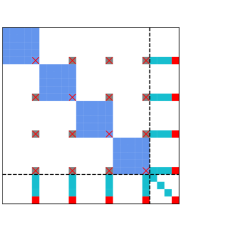
Figure 1: Sparsity pattern of the matrix $\hat{\underline{\bm{\mathcal{H}}}}$ for the case of four ion species, $N_{i}=4$.

The sparsity pattern of the matrix $\hat{\underline{\bm{\mathcal{H}}}}$ is displayed in Figure 1 in the case of four ion species ($N_{i}=4$). The blue diagonal blocks contain the hydrodynamic quantities of each ion species $\underline{\mathbf{A}}_{k}$. The gray off-diagonal entries contain $\overline{E}_{\mathrm{mag}}^{2}$, i.e., the single entry of $\underline{\mathbf{A}}_{\text{off}}$, which indicates how the energy equation for each ion species depends on the entropy variables associated with the energy of all other ion species. The entries in cyan are associated with the entropy variables pertinent to the magnetic field (non-zero rows of $\underline{\mathbf{B}}_{\text{off}}$) or the induction equations (diagonal of $\underline{\bm{\mathcal{C}}}$). Lastly, the red entries are dedicated to terms that encompass GLM-terms only, whereas the entries marked with a red cross include terms depending on GLM along with other terms. The dashed lines indicate the borders between the different blocks $\underline{\bm{\mathcal{A}}}$, $\underline{\bm{\mathcal{B}}}$, $\underline{\bm{\mathcal{B}}}^{T}$, and $\underline{\bm{\mathcal{C}}}$.

The matrix $\hat{\underline{\bm{\mathcal{H}}}}$ is consistent with the dissipation matrix of single-fluid MHD [54, 21] in the limit of one ion species $N_{i}=1$, and it produces a dissipation operator that is asymptotically consistent with the LLF dissipation operator, as shown in the Numerical Results section. The following lemma establishes the symmetric positive definiteness (SPD) of $\hat{\underline{\bm{\mathcal{H}}}}$ for an arbitrary number of species $N_{i}$. Our numerical experiments have consistently demonstrated entropy dissipation when utilizing it, as is detailed in the Numerical Results, Section 4.

Lemma 1.

The matrix $\hat{\underline{\bm{\mathcal{H}}}}$ defined in (68) is symmetric positive definite.

Proof.

The matrix $\hat{\underline{\bm{\mathcal{H}}}}$ is evidently symmetric. To show positive definiteness, we employ the Schur complement. Since the densities and pressures of all ion species are positive, i.e. $\rho_{k},p_{k}>0\,\forall k$, we have that $\beta_{k}:=\rho_{k}/2p_{k}>0$, $\beta_{+}:=\sum_{k}\beta_{k}>0$ and $\tau^{+}:=1/2\left\{\left\{\beta_{+}\right\}\right\}>0$. Thus, $\underline{\bm{\mathcal{C}}}$ is invertible and by Schur’s complement, cf. [55], $\hat{\underline{\bm{\mathcal{H}}}}$ is PD if and only if $\underline{\bm{\mathcal{C}}}$ is PD and its complement $\hat{\underline{\bm{\mathcal{H}}}}\setminus\underline{\bm{\mathcal{C}}}=\underline{\bm{\mathcal{A}}}-\underline{\bm{\mathcal{B}}}\underline{\bm{\mathcal{C}}}^{-1}\underline{\bm{\mathcal{B}}}^{T}$ is PD. By assumption, the fourfold eigenvalue, $\tau^{+}$, of $\underline{\bm{\mathcal{C}}}$ is strictly positive and, hence, $\underline{\bm{\mathcal{C}}}$ is PD and invertible with $\underline{\bm{\mathcal{C}}}^{-1}=\text{diag}(1/\tau^{+},1/\tau^{+},1/\tau^{+},1/\tau^{+})$. Thus,

$$(\underline{\bm{\mathcal{B}}}\underline{\bm{\mathcal{C}}}^{-1}\underline{\bm{\mathcal{B}}}^{T})_{i,j} =\begin{cases}\frac{1}{\tau^{+}}\tau^{+}\left(\left\{\left\{\vec{B}\right\}\right\}^{T},{\color[rgb]{1,0,0}\left\{\left\{\psi\right\}\right\}}\right)\cdot\tau^{+}\begin{pmatrix}\left\{\left\{\vec{B}\right\}\right\}\\ {\color[rgb]{1,0,0}\left\{\left\{\psi\right\}\right\}}\end{pmatrix}&\text{ if }i,j\!\!\!\!\mod 5=0,\\ 0&\text{otherwise}\end{cases}$$

$$=\begin{cases}\overline{E}_{\mathrm{mag}}^{2}&\text{ if }i,j\!\!\!\!\mod 5=0,\\ 0&\text{otherwise}\end{cases},$$

where we use the definition of $\overline{E}_{\mathrm{mag}}^{2}$ in Eq. (70). The non-zero positions of this matrix are exactly those marked with a red cross in Figure 1. Therefore, the complement $\hat{\underline{\bm{\mathcal{H}}}}\setminus\underline{\bm{\mathcal{C}}}=\text{diag}(\widetilde{\underline{\mathbf{A}}}_{1},\ldots,\widetilde{\underline{\mathbf{A}}}_{N_{i}})$ is a block-diagonal matrix with

$$\widetilde{\underline{\mathbf{A}}}_{k,(i,j)}=\begin{cases}\underline{\mathbf{A}}_{k,(i,j)}&\text{ if }(i,j)\neq(5,5),\\ \hat{\underline{\bm{\mathcal{H}}}}_{k,(5,5)}-\overline{E}_{\mathrm{mag}}^{2}&\text{ otherwise}.\end{cases}$$

We remark that the Schur complement matrix, $\hat{\underline{\bm{\mathcal{H}}}}\setminus\underline{\bm{\mathcal{C}}}$, is nothing but the dissipation matrix of the multi-species Euler system with a similar energy term. To show its positive definiteness, we can decompose it as $\widetilde{\underline{\mathbf{L}}}\,\widetilde{\underline{\mathbf{D}}}\,\widetilde{\underline{\mathbf{L}}}^{T}$, where $\widetilde{\underline{\mathbf{D}}}$ is a diagonal matrix that only contains positive entries. The $\widetilde{\underline{\mathbf{L}}}\,\widetilde{\underline{\mathbf{D}}}\,\widetilde{\underline{\mathbf{L}}}^{T}$ decomposition of each diagonal block $\widetilde{\underline{\mathbf{A}}}_{k}$ reads:

$$\widetilde{\underline{\mathbf{L}}}_{k}=\left(\begin{array}[]{ccccc}1&0&0&0&0\\ \left\{\left\{v_{k,1}\right\}\right\}&1&0&0&0\\ \left\{\left\{v_{k,2}\right\}\right\}&0&1&0&0\\ \left\{\left\{v_{k,3}\right\}\right\}&0&0&1&0\\ \frac{\overline{E}_{k}^{2}}{\rho_{k}^{\ln}}&\left\{\left\{v_{k,1}\right\}\right\}&\left\{\left\{v_{k,2}\right\}\right\}&\left\{\left\{v_{k,3}\right\}\right\}&1\end{array}\right),\ \widetilde{\underline{\mathbf{D}}}_{k}=\left(\begin{array}[]{ccccc}\rho_{k}^{\ln}&0&0&0&0\\ 0&\overline{p}_{k}&0&0&0\\ 0&0&\overline{p}_{k}&0&0\\ 0&0&0&\overline{p}_{k}&0\\ 0&0&0&0&\widetilde{\underline{\mathbf{A}}}_{k,(5,5)}\!\!-\overline{p}_{k}\left\lVert\left\{\left\{\vec{v_{k}}\right\}\right\}\right\rVert^{2}\!\!-\frac{\overline{E}_{k}^{2}}{\rho_{k}^{\ln}}\end{array}\right),$$ (71)

where

$$\widetilde{\underline{\mathbf{A}}}_{k,(5,5)}-\overline{p}_{k}\left\lVert\left\{\left\{\vec{v_{k}}\right\}\right\}\right\rVert^{2}-\frac{\overline{E}_{k}^{2}}{\rho_{k}^{\ln}}=\frac{1}{\rho_{k}^{\ln}}\frac{(p_{k}^{*})^{2}}{\gamma_{k}-1}>0$$

by assumption. Therefore, $\hat{\underline{\bm{\mathcal{H}}}}\setminus\underline{\bm{\mathcal{C}}}$ consists of diagonal blocks each having strictly positive eigenvalues, which implies that $\hat{\underline{\bm{\mathcal{H}}}}$ is SPD. ∎

Remark 3.

By Lemma 1 and Sylvester’s criterion, it is clear that the matrix $\underline{\bm{\mathcal{A}}}$ defined in (68), i.e the left upper diagonal block of $\hat{\underline{\bm{\mathcal{H}}}}$, is SPD. However, we would like to state an additional direct proof of this fact since some of techniques used therein seem noteworthy.

Proof.

We make the same assumptions as in the proof of Lemma 1. In addition, let $\overline{E}_{\mathrm{mag}}^{2}\neq 0$, otherwise $\underline{\bm{\mathcal{A}}}$ has a simple block-diagonal structure and it is easy to confirm that it is SPD. The $\underline{\mathbf{L}}\underline{\mathbf{D}}\underline{\mathbf{L}}^{T}$ decomposition of each diagonal block $\underline{\mathbf{A}}_{k}$ is the same as in (71), except for the last eigenvalue that reads $\underline{\mathbf{D}}_{k,(5,5)}=\hat{\mathcal{H}}_{k,(E_{k},E_{k})}-\overline{p}_{k}\left\lVert\left\{\left\{\vec{v_{k}}\right\}\right\}\right\rVert^{2}-\frac{\overline{E}_{k}^{2}}{\rho_{k}^{\ln}}$.

Let $\underline{\bm{\mathcal{L}}}=\text{diag}(\underline{\mathbf{L}}_{1},\ldots,\underline{\mathbf{L}}_{N_{i}})$ be a block diagonal matrix and consider the similarity transformation $\underline{\bm{\mathcal{A}}}^{\prime}:=\underline{\bm{\mathcal{L}}}^{-1}\underline{\bm{\mathcal{A}}}\underline{\bm{\mathcal{L}}}^{-T}$. The inverse of $\underline{\bm{\mathcal{L}}}$ exists since its diagonal blocks $\underline{\mathbf{L}}_{k}$ are invertible. The transformation of the off-diagonal blocks of $\underline{\bm{\mathcal{A}}}$ is obtained as follows:

$$\underline{\mathbf{L}}^{-1}_{k}\cdot\begin{pmatrix}0&\cdots&0\\ \vdots&\ddots&0\\ 0&\cdots&\overline{E}_{\mathrm{mag}}^{2}\end{pmatrix}\stackrel{{\scriptstyle!}}{{=}}\begin{pmatrix}0&\cdots&0&\vdots\\ \vdots&\ddots&\vdots&\mathbf{c}\\ 0&\cdots&0&\vdots\end{pmatrix}\,\,\Leftrightarrow\,\,\underline{\mathbf{L}}_{k}\mathbf{c}=\begin{pmatrix}0\\ \vdots\\ 0\\ \overline{E}_{\mathrm{mag}}^{2}\end{pmatrix}$$

where $\mathbf{c}\in\mathbb{R}^{5}$. Forwards substitution yields $\mathbf{c}=\left(0,\ldots,0,\overline{E}_{\mathrm{mag}}^{2}\right)^{T}$. The same holds for the right-hand-side case due to symmetry and transposition rules of matrix-vector products.

Thus, the off-diagonal blocks $\underline{\mathbf{A}}_{\text{off}}$ of $\underline{\bm{\mathcal{A}}}$ are invariant under this similarity transformation and $\underline{\bm{\mathcal{A}}}^{\prime}$ has an almost diagonal structure:

$$\underline{\bm{\mathcal{A}}}^{\prime}[5k-4,\ldots,5k;\,5k-4,\ldots,5k]=\underline{\mathbf{D}}_{k},\quad\underline{\bm{\mathcal{A}}}^{\prime}_{(5i,5j)}=\overline{E}_{\mathrm{mag}}^{2}\quad\text{for }i\neq j,\,i,j\in\{1,\ldots,N_{i}\}$$

and $\underline{\bm{\mathcal{A}}}^{\prime}$ is zero everywhere else. Next, we show that $\underline{\bm{\mathcal{A}}}^{\prime}$ is SPD. Let $\mathbf{x}\in\mathbb{R}^{5N_{i}}$, such that $\mathbf{x}\neq\mathbf{0}$, then:

$$\mathbf{x}^{T}\underline{\bm{\mathcal{A}}}^{\prime}\mathbf{x}= \sum_{i=1}^{5N_{i}}x_{i}^{2}\underline{\mathbf{D}}_{i\text{ div }5,(i\!\!\!\!\mod 5,\,i\!\!\!\!\mod 5)}+\overline{E}_{\mathrm{mag}}^{2}\sum_{k=1}^{N_{i}}x_{5j}\sum_{l=1,l\neq k}^{N_{i}}x_{5l}$$

$$= \sum_{k=1}^{N_{i}}\sum_{m=1}^{4}x_{5(k-1)+m}^{2}\underline{\mathbf{D}}_{k,(m,m)}+\sum_{k=1}^{N_{i}}x_{5k}^{2}(\underline{\mathbf{D}}_{k,(5k,5k)}-\overline{E}_{\mathrm{mag}}^{2})+\sum_{k=1}^{N_{i}}\overline{E}_{\mathrm{mag}}^{2}x_{5k}^{2}+\overline{E}_{\mathrm{mag}}^{2}\sum_{k=1}^{N_{i}}x_{5j}\sum_{l=1,l\neq k}^{N_{i}}x_{5l}$$

$$= \sum_{k=1}^{N_{i}}\sum_{m=1}^{4}x_{5(k-1)+m}^{2}\underline{\mathbf{D}}_{k,(m,m)}+\sum_{k=1}^{N_{i}}x_{5k}^{2}(\underline{\mathbf{D}}_{k,(5k,5k)}-\overline{E}_{\mathrm{mag}}^{2})+\overline{E}_{\mathrm{mag}}^{2}\left(\sum_{k=1}^{N_{i}}x_{5j}\right)^{2}$$

Since $\overline{E}_{\mathrm{mag}}^{2}>0$ and the eigenvalues of $\underline{\bm{\mathcal{A}}}$ are non-negative, it is left to show that the second summand is non-negative for any $k\in\{1,\ldots,N_{i}\}$:

$$\underline{\mathbf{D}}_{k,(5k,5k)}-\overline{E}_{\mathrm{mag}}^{2}=\hat{\mathcal{H}}_{k,(5,5)}\!\!-\overline{p}_{k}\left\lVert\left\{\left\{\vec{v_{k}}\right\}\right\}\right\rVert^{2}\!\!-\frac{\overline{E}_{k}^{2}}{\rho_{k}^{\ln}}-\overline{E}_{\mathrm{mag}}^{2}\stackrel{{\scriptstyle\eqref{eq:H_k_EnergyTerm}}}{{=}}\frac{1}{\rho_{k}^{\ln}}\frac{(p_{k}^{*})^{2}}{\gamma_{k}-1}>0,$$

Thus, $\underline{\bm{\mathcal{A}}}^{\prime}$ and its similar transform, $\underline{\bm{\mathcal{A}}}$, are SPD. ∎

3.2.2 Standard Rusanov Numerical Flux

The flux derived in Section 3.2.1 requires the computation of the entropy Jacobian. Another (simpler) possibility is to use a standard Rusanov (LLF) numerical flux function at the element interfaces,

$${\hat{\mathbf{f}}}_{(L,R)} =\left\{\left\{\mathbf{f}\right\}\right\}_{(L,R)}-\frac{1}{2}\lambda^{\max}_{(L,R)}\left\llbracket\mathbf{u}\right\rrbracket_{(L,R)},$$ (72)

$$\bm{\Phi}^{\diamond}_{(L,R)} =\bm{\phi}_{L}^{{\mathrm{GP}}}\left\{\left\{B_{1}\right\}\right\}_{(L,R)}+\bm{\phi}_{L}^{\rm{Lor}}\circ\left\{\left\{\mathbf{h}^{\rm{Lor}}\right\}\right\}_{(L,R)}+\vec{B}_{L}\cdot\left\{\left\{\accentset{\,\leftrightarrow}{{\mathbf{h}}}^{\rm{multi}}\right\}\right\}_{(L,R)}+{\color[rgb]{1,0,0}\bm{\phi}_{L}^{\rm{GLM}}\left\{\left\{\psi\right\}\right\}_{(L,R)}}.$$ (73)

While the standard LLF flux has demonstrated entropy stability for various conservative and non-conservative systems such as the Euler equations [59], shallow water magnetohydrodynamics equations [63], and relativistic hydrodynamics equations [64], among many others given an accurate estimation of $\lambda^{\max}$ from above, there is currently no formal proof establishing its entropy stability for the multi-ion GLM-MHD system to the authors’ knowledge. It is noteworthy, however, that our numerical tests revealed entropy dissipation and robust performance of this flux function for all performed simulations, as elaborated in the Numerical Results section.

A Note on the Maximum Wave Speed:

As pointed out by Tóth et al. [65], the explicit formulas for the wave modes and wave speeds of the multi-ion MHD system are unfortunately not known, as the generalization to $N_{i}$ ion species is not trivial. In this work, we use a similar approach to the one of the BATS-R-US code [65, 5], and estimate the maximum wave speeds with a generalization of the single-fluid wave speeds. In particular, for the dissipation operator of the numerical flux function we use

$$\lambda^{\max}_{(L,R)}\approx\max\left[\left(\max_{k=1,\ldots,N_{i}}\vec{v}_{k}\cdot\vec{n}_{(L,R)}\right)_{L},\left(\max_{k=1,\ldots,N_{i}}\vec{v}_{k}\cdot\vec{n}_{(L,R)}\right)_{R}\right]+\max\left[c_{f}\left(\mathbf{u}_{L},\vec{n}_{(L,R)}\right),c_{f}\left(\mathbf{u}_{R},\vec{n}_{(L,R)}\right)\right],$$ (74)

where $\vec{n}_{(L,R)}$ is the normal vector at the interface $(L,R)$, and the multi-ion fast magneto-sonic speed is estimated with a generalization of the single-fluid speeds:

$$c_{f}^{2}\left(\mathbf{u},\vec{n}\right)=\max_{k=1,\ldots,N_{i}}\frac{1}{2}\left(a^{2}+\|\vec{b}\|^{2}+\sqrt{(a^{2}+\|\vec{b}\|^{2})^{2}-4a^{2}(\vec{b}\cdot\vec{n})^{2}}\right),~{}~{}~{}a^{2}=\gamma_{k}\frac{p_{k}}{\rho_{k}},~{}~{}~{}\vec{b}=\frac{\vec{B}}{\rho}.$$ (75)

Similarly, to compute the explicit time-step size, we compute a two-dimensional nodal maximum wave speed as

$$\lambda^{\max}=\max_{k=1,\ldots,N_{i}}v_{k,1}+c_{f}\left(\mathbf{u},\vec{n}_{1}\right)+\max_{k=1,\ldots,N_{i}}v_{k,2}+c_{f}\left(\mathbf{u},\vec{n}_{2}\right),$$ (76)

where the unit vectors are defined as $\vec{n}_{1}=(1,0,0)$ and $\vec{n}_{2}=(0,1,0)$.

4 Numerical Results

In this section, we test the numerical accuracy, entropy consistency, and robustness of our entropy-stable LGL-DGSEM discretization of the multi-ion GLM-MHD equations. For simplicity, we will focus on two-dimensional test cases on Cartesian meshes, but the methods of this paper can be extended to three-dimensional problems on curvilinear meshes, as shown in [41, 56, 44].

In all cases, the time integration was performed with the explicit fourth-order five-stages Runge-Kutta (RK4-5) scheme of Carpenter and Kennedy [66]. The time-step size is estimated as in [67],

$$\Delta t=\min_{i,j}\left(\frac{\mathrm{CFL}}{(N+1)}\frac{h}{\lambda_{ij}^{\max}}\right),$$ (77)

where $h$ is the element size, the nodal maximum wave speed $\lambda^{\max}_{ij}$ is computed using (76), and we use CFL$=0.5$ for all cases, unless otherwise stated.

At each time step, we compute the explicit time-step size using (77), and then compute the divergence cleaning speed, such that the GLM technique does not affect the stability of the method:

$${\color[rgb]{1,0,0}c_{h}=\frac{\nu}{\Delta t}\underbrace{\frac{\mathrm{CFL}\,h}{2(N+1)}}_{\Delta t_{c_{h}}},}$$ (78)

where $\Delta t_{c_{h}}$ is the explicit time-step size that corresponds to $c_{h}=1$ and $\nu$ is a scaling constant that we choose as $\nu=0.5$.

All the simulations of this section were run with the two-dimensional Cartesian TreeMesh solver of the open-source framework Trixi.jl [68, 69, 67].

4.1 Convergence Test

To test the convergence properties of the new schemes, we solve a manufactured solution test case for a two-species collisionless plasma. We assume an exact solution to the ideal multi-ion GLM-MHD system of the form

$$\rho_{1}(\vec{x},t) =h_{1}, \rho_{2}(\vec{x},t) =h_{2},$$

$$\rho_{1}v_{1,1}(\vec{x},t) =h_{1}, \rho_{2}v_{2,1}(\vec{x},t) =h_{2},$$

$$\rho_{1}v_{1,2}(\vec{x},t) =h_{1}, \rho_{2}v_{2,2}(\vec{x},t) =h_{2},$$

$$\rho_{1}v_{1,3}(\vec{x},t) =0.1*h_{1}, \rho_{2}v_{2,3}(\vec{x},t) =0.1*h_{2},$$

$$E_{1}(\vec{x},t) =2*h_{1}^{2}+h_{1}, E_{2}(\vec{x},t) =2*h_{2}^{2}+h_{2},$$

$$B_{1}(\vec{x},t) =0.25*h, B_{2}(\vec{x},t) =-0.25*h,$$

$$B_{3}(\vec{x},t) =0.1*h, {\color[rgb]{1,0,0}\psi(\vec{x},t)} {\color[rgb]{1,0,0}=0,}$$ (79)

with the auxiliary variables

$$h =\underbrace{0.1*\sin(\pi*(x+y-t))}_{:=h_{0}}+2,$$

$$h_{1} =0.1*0.4*\sin(\pi*(x+y-t))+1,$$

$$h_{2} =h-h_{1}.$$

To consider important multi-ion effects, we use different heat capacity ratios for the two ion species, $\gamma_{1}=2$ and $\gamma_{2}=4$, and also different charge-to-mass rations, $r_{1}=2$ and $r_{2}=1$. Moreover, we use a non-trivial electron pressure to test the convergence properties of our scheme using all the terms of the equation. In particular, we use [1]

$$p_{e}=\alpha\sum_{k=1}^{N_{i}}p_{k},$$ (80)

with $\alpha\neq 0$. Equation (80) is equivalent to taking the electron pressure gradient term in the momentum and energy equations to be equal to a fraction of the total ion pressure gradient. For the numerical experiments of this section, we use $\alpha=0.2$, but we would like to remark that the choice of $\alpha$ depends on the application. For instance, Glocer et al. [5] used $\alpha=0.2$ for simulations of the interaction of the solar wind with Earth’s magnetosphere, whereas Najib et al. [70] used a value of $\alpha=1$ to simulate the interaction of the solar wind with mars.

We insert (4.1) into (2.4) and use the symbolic algebra tool Maxima [71] to obtain the source term:

$$\mathbf{s}=\begin{pmatrix}\frac{2\,h_{x}}{5}\\ \frac{38055\,h_{x}\,h_{0}^{2}+185541\,h_{x}\,h_{0}+220190\,h_{x}}{35000\,h_{0}+75000}\\ \frac{38055\,h_{x}\,h_{0}^{2}+185541\,h_{x}\,h_{0}+220190\,h_{x}}{35000\,h_{0}+75000}\\ \frac{h_{x}}{25}\\ \frac{1835811702576186755\,h_{x}\,h_{0}^{2}+8592627463681183181\,h_{x}\,h_{0}+9884050459977240490\,h_{x}}{652252660543767500\,h_{0}+1397684272593787500}\\ \frac{3\,h_{x}}{5}\\ \frac{76155\,h_{x}\,h_{0}^{2}+295306\,h_{x}\,h_{0}+284435\,h_{x}}{17500\,h_{0}+37500}\\ \frac{76155\,h_{x}\,h_{0}^{2}+295306\,h_{x}\,h_{0}+284435\,h_{x}}{17500\,h_{0}+37500}\\ \frac{3\,h_{x}}{50}\\ \frac{88755\,h_{x}\,h_{0}^{2}+338056\,h_{x}\,h_{0}+318185\,h_{x}}{8750\,h_{0}+18750}\\ \frac{h_{x}}{4}\\ \frac{-h_{x}}{4}\\ \frac{h_{x}}{10}\\ {\color[rgb]{1,0,0}0}\end{pmatrix}.$$ (81)

Equation (81) shows that the source term required to derive the manufactured solution (4.1) is highly intricate. This complexity arises from the intricate interdependencies among ions and the nonlinearities inherent in the ideal multi-ion GLM-MHD system.

We solve the multi-ion GLM-MHD system with the initial condition given by (4.1) and the source term (81) in the domain $\Omega=[-1,1]^{2}$ with periodic boundary conditions, the final time $t_{f}=1$, and three different solvers:

1. EC: A split-form entropy-conservative LGL-DGSEM that uses the EC fluxes and non-conservative terms (55)-(60) in both the volume and surface numerical fluxes and terms of (61),

2. ES: A split-form provably entropy-stable LGL-DGSEM that uses the EC fluxes and non-conservative terms (55)-(60) in the volume numerical fluxes and non-conservative terms, and the entropy-dissipative LLF-like fluxes and non-conservative term (3.2.1) in the surface numerical fluxes and terms of (61), and

3. EC+LLF: A dissipative split-form LGL-DGSEM that uses the EC fluxes and non-conservative terms (55)-(60) in the volume numerical fluxes and non-conservative terms, and the standard LLF solver (72) in the surface numerical fluxes and terms of (61).

Tables 1 to 4 show the errors and experimental orders of convergence (EOCs) obtained with the EC LGL-DGSEM solver (i) for the manufactured solution test at time $t_{f}=1$. We observe high-order convergence, but also an even-odd effect, in which even polynomial degrees exhibit an optimal convergence order of approximately $\mathcal{O}(N+1)$ and odd polynomial degrees exhibit a sub-optimal convergence order of approximately $\mathcal{O}(N)$. This effect has been observed for EC discretizations of other equations, e.g. [72, 35].

Tables 5 to 8 show the errors and experimental orders of convergence (EOCs) obtained with the ES (ii) and EC+LLF (iii) solvers for the manufactured solution test at time $t_{f}=1$. The experimental orders of convergence and the errors are identical for the solver (iii) and the solver (ii) for the precision shown.

With solvers (ii) and (iii), we observe high-order convergence without any even-odd effect. All polynomial degrees exhibit an optimal convergence order of approximately $\mathcal{O}(N+1)$.

Table 1: $L_{2}$ errors and EOCs for the convergence test with the EC scheme (i) for $N=2$ and different numbers of elements per direction $N_{e}$.

$N_{e}$	$\left\lVert\epsilon_{B_{1}}\right\rVert$	EOC	$\left\lVert\epsilon_{B_{2}}\right\rVert$	EOC	$\left\lVert\epsilon_{B_{3}}\right\rVert$	EOC	$\left\lVert\epsilon_{\rho_{1}}\right\rVert$	EOC	$\left\lVert\epsilon_{\rho_{1}v_{1,1}}\right\rVert$	EOC	$\left\lVert\epsilon_{\rho_{1}v_{1,2}}\right\rVert$	EOC	$\left\lVert\epsilon_{\rho_{1}v_{1,3}}\right\rVert$	EOC
$16$	$1.39\times 10^{-5}$	$-$	$1.39\times 10^{-5}$	$-$	$4.17\times 10^{-6}$	$-$	$2.23\times 10^{-5}$	$-$	$3.55\times 10^{-5}$	$-$	$3.55\times 10^{-5}$	$-$	$6.20\times 10^{-6}$	$-$
$32$	$1.64\times 10^{-6}$	$3.09$	$1.64\times 10^{-6}$	$3.08$	$7.18\times 10^{-7}$	$2.54$	$3.72\times 10^{-6}$	$2.58$	$4.54\times 10^{-6}$	$2.97$	$4.55\times 10^{-6}$	$2.96$	$4.87\times 10^{-7}$	$3.67$
$64$	$1.76\times 10^{-7}$	$3.22$	$1.76\times 10^{-7}$	$3.22$	$8.47\times 10^{-8}$	$3.08$	$3.38\times 10^{-7}$	$3.46$	$4.01\times 10^{-7}$	$3.50$	$4.01\times 10^{-7}$	$3.50$	$5.61\times 10^{-8}$	$3.12$
$128$	$3.91\times 10^{-8}$	$2.17$	$3.91\times 10^{-8}$	$2.17$	$1.23\times 10^{-8}$	$2.78$	$4.88\times 10^{-8}$	$2.79$	$7.53\times 10^{-8}$	$2.41$	$7.53\times 10^{-8}$	$2.41$	$6.70\times 10^{-9}$	$3.07$
mean		$2.83$		$2.82$		$2.80$		$2.94$		$2.96$		$2.96$		$3.29$
$N_{e}$	$\left\lVert\epsilon_{E_{1}}\right\rVert$	EOC	$\left\lVert\epsilon_{\rho_{2}}\right\rVert$	EOC	$\left\lVert\epsilon_{\rho_{2}v_{2,1}}\right\rVert$	EOC	$\left\lVert\epsilon_{\rho_{2}v_{2,2}}\right\rVert$	EOC	$\left\lVert\epsilon_{\rho_{2}v_{2,3}}\right\rVert$	EOC	$\left\lVert\epsilon_{E_{2}}\right\rVert$	EOC	$\left\lVert\epsilon_{\psi}\right\rVert$	EOC
$16$	$1.10\times 10^{-4}$	$-$	$3.12\times 10^{-5}$	$-$	$7.37\times 10^{-5}$	$-$	$7.37\times 10^{-5}$	$-$	$1.58\times 10^{-5}$	$-$	$1.79\times 10^{-4}$	$-$	$5.56\times 10^{-6}$	$-$
$32$	$1.79\times 10^{-5}$	$2.62$	$3.71\times 10^{-6}$	$3.07$	$6.11\times 10^{-6}$	$3.59$	$6.10\times 10^{-6}$	$3.59$	$8.59\times 10^{-7}$	$4.21$	$1.48\times 10^{-5}$	$3.59$	$1.51\times 10^{-6}$	$1.88$
$64$	$1.54\times 10^{-6}$	$3.54$	$4.58\times 10^{-7}$	$3.02$	$7.02\times 10^{-7}$	$3.12$	$7.02\times 10^{-7}$	$3.12$	$5.40\times 10^{-8}$	$3.99$	$1.97\times 10^{-6}$	$2.92$	$1.79\times 10^{-7}$	$3.08$
$128$	$2.81\times 10^{-7}$	$2.46$	$6.45\times 10^{-8}$	$2.83$	$9.76\times 10^{-8}$	$2.85$	$9.76\times 10^{-8}$	$2.85$	$5.88\times 10^{-9}$	$3.20$	$3.49\times 10^{-7}$	$2.50$	$9.87\times 10^{-9}$	$4.18$
mean		$2.87$		$2.97$		$3.19$		$3.19$		$3.80$		$3.00$		$3.05$

Table 2: $L_{2}$ errors and EOCs for the convergence test with the EC scheme (i) for $N=3$ and different numbers of elements per direction $N_{e}$.

$N_{e}$	$\left\lVert\epsilon_{B_{1}}\right\rVert$	EOC	$\left\lVert\epsilon_{B_{2}}\right\rVert$	EOC	$\left\lVert\epsilon_{B_{3}}\right\rVert$	EOC	$\left\lVert\epsilon_{\rho_{1}}\right\rVert$	EOC	$\left\lVert\epsilon_{\rho_{1}v_{1,1}}\right\rVert$	EOC	$\left\lVert\epsilon_{\rho_{1}v_{1,2}}\right\rVert$	EOC	$\left\lVert\epsilon_{\rho_{1}v_{1,3}}\right\rVert$	EOC
$8$	$1.09\times 10^{-4}$	$-$	$1.09\times 10^{-4}$	$-$	$1.42\times 10^{-5}$	$-$	$4.19\times 10^{-5}$	$-$	$9.53\times 10^{-5}$	$-$	$9.53\times 10^{-5}$	$-$	$2.28\times 10^{-5}$	$-$
$16$	$1.17\times 10^{-5}$	$3.22$	$1.17\times 10^{-5}$	$3.22$	$1.43\times 10^{-6}$	$3.30$	$4.38\times 10^{-6}$	$3.26$	$1.02\times 10^{-5}$	$3.22$	$1.02\times 10^{-5}$	$3.23$	$2.77\times 10^{-6}$	$3.05$
$32$	$1.41\times 10^{-6}$	$3.06$	$1.41\times 10^{-6}$	$3.06$	$1.70\times 10^{-7}$	$3.08$	$5.12\times 10^{-7}$	$3.09$	$1.22\times 10^{-6}$	$3.07$	$1.21\times 10^{-6}$	$3.07$	$3.44\times 10^{-7}$	$3.01$
$64$	$1.74\times 10^{-7}$	$3.01$	$1.74\times 10^{-7}$	$3.01$	$2.09\times 10^{-8}$	$3.02$	$6.30\times 10^{-8}$	$3.02$	$1.50\times 10^{-7}$	$3.02$	$1.50\times 10^{-7}$	$3.02$	$4.29\times 10^{-8}$	$3.00$
mean		$3.10$		$3.10$		$3.13$		$3.12$		$3.10$		$3.11$		$3.02$
$N_{e}$	$\left\lVert\epsilon_{E_{1}}\right\rVert$	EOC	$\left\lVert\epsilon_{\rho_{2}}\right\rVert$	EOC	$\left\lVert\epsilon_{\rho_{2}v_{2,1}}\right\rVert$	EOC	$\left\lVert\epsilon_{\rho_{2}v_{2,2}}\right\rVert$	EOC	$\left\lVert\epsilon_{\rho_{2}v_{2,3}}\right\rVert$	EOC	$\left\lVert\epsilon_{E_{2}}\right\rVert$	EOC	$\left\lVert\epsilon_{\psi}\right\rVert$	EOC
$8$	$2.53\times 10^{-4}$	$-$	$5.44\times 10^{-5}$	$-$	$1.96\times 10^{-4}$	$-$	$1.96\times 10^{-4}$	$-$	$7.03\times 10^{-5}$	$-$	$5.36\times 10^{-4}$	$-$	$1.10\times 10^{-5}$	$-$
$16$	$2.74\times 10^{-5}$	$3.20$	$4.61\times 10^{-6}$	$3.56$	$2.17\times 10^{-5}$	$3.17$	$2.17\times 10^{-5}$	$3.17$	$8.08\times 10^{-6}$	$3.12$	$5.12\times 10^{-5}$	$3.39$	$1.92\times 10^{-7}$	$5.84$
$32$	$3.27\times 10^{-6}$	$3.07$	$5.30\times 10^{-7}$	$3.12$	$2.60\times 10^{-6}$	$3.06$	$2.61\times 10^{-6}$	$3.06$	$9.90\times 10^{-7}$	$3.03$	$6.04\times 10^{-6}$	$3.09$	$1.56\times 10^{-8}$	$3.63$
$64$	$4.04\times 10^{-7}$	$3.02$	$6.52\times 10^{-8}$	$3.02$	$3.21\times 10^{-7}$	$3.01$	$3.23\times 10^{-7}$	$3.01$	$1.23\times 10^{-7}$	$3.01$	$7.45\times 10^{-7}$	$3.02$	$3.10\times 10^{-9}$	$2.33$
mean		$3.10$		$3.23$		$3.08$		$3.08$		$3.05$		$3.17$		$3.93$

Table 3: $L_{2}$ errors and EOCs for the convergence test with the EC scheme (i) for $N=4$ and different numbers of elements per direction $N_{e}$.

$N_{e}$	$\left\lVert\epsilon_{B_{1}}\right\rVert$	EOC	$\left\lVert\epsilon_{B_{2}}\right\rVert$	EOC	$\left\lVert\epsilon_{B_{3}}\right\rVert$	EOC	$\left\lVert\epsilon_{\rho_{1}}\right\rVert$	EOC	$\left\lVert\epsilon_{\rho_{1}v_{1,1}}\right\rVert$	EOC	$\left\lVert\epsilon_{\rho_{1}v_{1,2}}\right\rVert$	EOC	$\left\lVert\epsilon_{\rho_{1}v_{1,3}}\right\rVert$	EOC
$8$	$4.97\times 10^{-7}$	$-$	$4.97\times 10^{-7}$	$-$	$5.78\times 10^{-8}$	$-$	$2.61\times 10^{-7}$	$-$	$4.87\times 10^{-7}$	$-$	$4.87\times 10^{-7}$	$-$	$1.24\times 10^{-7}$	$-$
$16$	$6.77\times 10^{-9}$	$6.20$	$6.77\times 10^{-9}$	$6.20$	$1.97\times 10^{-9}$	$4.88$	$7.79\times 10^{-9}$	$5.07$	$1.35\times 10^{-8}$	$5.17$	$1.35\times 10^{-8}$	$5.17$	$1.97\times 10^{-9}$	$5.98$
$32$	$1.61\times 10^{-10}$	$5.40$	$1.61\times 10^{-10}$	$5.40$	$6.95\times 10^{-11}$	$4.82$	$3.35\times 10^{-10}$	$4.54$	$4.20\times 10^{-10}$	$5.00$	$4.20\times 10^{-10}$	$5.00$	$5.31\times 10^{-11}$	$5.21$
$64$	$5.04\times 10^{-12}$	$4.99$	$5.04\times 10^{-12}$	$4.99$	$1.92\times 10^{-12}$	$5.18$	$1.02\times 10^{-11}$	$5.04$	$1.44\times 10^{-11}$	$4.87$	$1.44\times 10^{-11}$	$4.86$	$1.16\times 10^{-12}$	$5.52$
mean		$5.53$		$5.53$		$4.96$		$4.88$		$5.01$		$5.01$		$5.57$
$N_{e}$	$\left\lVert\epsilon_{E_{1}}\right\rVert$	EOC	$\left\lVert\epsilon_{\rho_{2}}\right\rVert$	EOC	$\left\lVert\epsilon_{\rho_{2}v_{2,1}}\right\rVert$	EOC	$\left\lVert\epsilon_{\rho_{2}v_{2,2}}\right\rVert$	EOC	$\left\lVert\epsilon_{\rho_{2}v_{2,3}}\right\rVert$	EOC	$\left\lVert\epsilon_{E_{2}}\right\rVert$	EOC	$\left\lVert\epsilon_{\psi}\right\rVert$	EOC
$8$	$1.15\times 10^{-6}$	$-$	$3.64\times 10^{-7}$	$-$	$6.03\times 10^{-7}$	$-$	$6.03\times 10^{-7}$	$-$	$1.98\times 10^{-7}$	$-$	$2.08\times 10^{-6}$	$-$	$9.89\times 10^{-8}$	$-$
$16$	$2.93\times 10^{-8}$	$5.30$	$1.23\times 10^{-8}$	$4.88$	$2.26\times 10^{-8}$	$4.74$	$2.26\times 10^{-8}$	$4.74$	$3.97\times 10^{-9}$	$5.64$	$5.72\times 10^{-8}$	$5.18$	$6.05\times 10^{-9}$	$4.03$
$32$	$1.56\times 10^{-9}$	$4.23$	$3.84\times 10^{-10}$	$5.01$	$7.07\times 10^{-10}$	$5.00$	$7.07\times 10^{-10}$	$5.00$	$4.89\times 10^{-11}$	$6.34$	$2.17\times 10^{-9}$	$4.72$	$1.20\times 10^{-10}$	$5.66$
$64$	$4.96\times 10^{-11}$	$4.97$	$1.59\times 10^{-11}$	$4.59$	$2.29\times 10^{-11}$	$4.95$	$2.29\times 10^{-11}$	$4.95$	$1.98\times 10^{-12}$	$4.63$	$7.23\times 10^{-11}$	$4.91$	$4.27\times 10^{-12}$	$4.81$
mean		$4.83$		$4.83$		$4.90$		$4.90$		$5.54$		$4.94$		$4.83$

Table 4: $L_{2}$ errors and EOCs for the convergence test with the EC scheme (i) for $N=5$ and different numbers of elements per direction $N_{e}$.

$N_{e}$	$\left\lVert\epsilon_{B_{1}}\right\rVert$	EOC	$\left\lVert\epsilon_{B_{2}}\right\rVert$	EOC	$\left\lVert\epsilon_{B_{3}}\right\rVert$	EOC	$\left\lVert\epsilon_{\rho_{1}}\right\rVert$	EOC	$\left\lVert\epsilon_{\rho_{1}v_{1,1}}\right\rVert$	EOC	$\left\lVert\epsilon_{\rho_{1}v_{1,2}}\right\rVert$	EOC	$\left\lVert\epsilon_{\rho_{1}v_{1,3}}\right\rVert$	EOC
$4$	$1.47\times 10^{-6}$	$-$	$1.47\times 10^{-6}$	$-$	$2.28\times 10^{-7}$	$-$	$1.26\times 10^{-6}$	$-$	$2.32\times 10^{-6}$	$-$	$2.29\times 10^{-6}$	$-$	$7.40\times 10^{-7}$	$-$
$8$	$4.47\times 10^{-8}$	$5.04$	$4.48\times 10^{-8}$	$5.03$	$8.50\times 10^{-9}$	$4.75$	$4.23\times 10^{-8}$	$4.90$	$1.02\times 10^{-7}$	$4.51$	$1.01\times 10^{-7}$	$4.51$	$1.52\times 10^{-8}$	$5.61$
$16$	$1.41\times 10^{-9}$	$4.99$	$1.41\times 10^{-9}$	$4.99$	$3.69\times 10^{-10}$	$4.53$	$1.56\times 10^{-9}$	$4.76$	$3.23\times 10^{-9}$	$4.97$	$3.21\times 10^{-9}$	$4.97$	$4.54\times 10^{-10}$	$5.06$
$32$	$4.43\times 10^{-11}$	$4.99$	$4.43\times 10^{-11}$	$4.99$	$1.17\times 10^{-11}$	$4.98$	$4.83\times 10^{-11}$	$5.01$	$9.87\times 10^{-11}$	$5.03$	$9.79\times 10^{-11}$	$5.03$	$1.43\times 10^{-11}$	$4.99$
mean		$5.01$		$5.00$		$4.75$		$4.89$		$4.84$		$4.84$		$5.22$
$N_{e}$	$\left\lVert\epsilon_{E_{1}}\right\rVert$	EOC	$\left\lVert\epsilon_{\rho_{2}}\right\rVert$	EOC	$\left\lVert\epsilon_{\rho_{2}v_{2,1}}\right\rVert$	EOC	$\left\lVert\epsilon_{\rho_{2}v_{2,2}}\right\rVert$	EOC	$\left\lVert\epsilon_{\rho_{2}v_{2,3}}\right\rVert$	EOC	$\left\lVert\epsilon_{E_{2}}\right\rVert$	EOC	$\left\lVert\epsilon_{\psi}\right\rVert$	EOC
$4$	$7.11\times 10^{-6}$	$-$	$1.24\times 10^{-6}$	$-$	$3.58\times 10^{-6}$	$-$	$3.63\times 10^{-6}$	$-$	$1.55\times 10^{-6}$	$-$	$1.23\times 10^{-5}$	$-$	$3.69\times 10^{-7}$	$-$
$8$	$2.80\times 10^{-7}$	$4.67$	$3.87\times 10^{-8}$	$5.00$	$1.52\times 10^{-7}$	$4.56$	$1.53\times 10^{-7}$	$4.56$	$4.10\times 10^{-8}$	$5.24$	$3.23\times 10^{-7}$	$5.26$	$5.94\times 10^{-9}$	$5.96$
$16$	$9.64\times 10^{-9}$	$4.86$	$2.10\times 10^{-9}$	$4.20$	$5.63\times 10^{-9}$	$4.76$	$5.66\times 10^{-9}$	$4.76$	$1.32\times 10^{-9}$	$4.96$	$1.61\times 10^{-8}$	$4.33$	$4.55\times 10^{-10}$	$3.71$
$32$	$2.91\times 10^{-10}$	$5.05$	$6.91\times 10^{-11}$	$4.93$	$1.75\times 10^{-10}$	$5.01$	$1.76\times 10^{-10}$	$5.01$	$4.12\times 10^{-11}$	$5.00$	$5.28\times 10^{-10}$	$4.93$	$1.37\times 10^{-11}$	$5.05$
mean		$4.86$		$4.71$		$4.78$		$4.78$		$5.07$		$4.84$		$4.91$

Table 5: $L_{2}$ errors and EOCs for the convergence test with the ES (ii) and EC+LLF (iii) schemes for $N=2$ and different numbers of elements per direction $N_{e}$.

$N_{e}$	$\left\lVert\epsilon_{B_{1}}\right\rVert$	EOC	$\left\lVert\epsilon_{B_{2}}\right\rVert$	EOC	$\left\lVert\epsilon_{B_{3}}\right\rVert$	EOC	$\left\lVert\epsilon_{\rho_{1}}\right\rVert$	EOC	$\left\lVert\epsilon_{\rho_{1}v_{1,1}}\right\rVert$	EOC	$\left\lVert\epsilon_{\rho_{1}v_{1,2}}\right\rVert$	EOC	$\left\lVert\epsilon_{\rho_{1}v_{1,3}}\right\rVert$	EOC
$16$	$2.03\times 10^{-5}$	$-$	$2.04\times 10^{-5}$	$-$	$1.11\times 10^{-5}$	$-$	$3.14\times 10^{-5}$	$-$	$9.23\times 10^{-5}$	$-$	$9.20\times 10^{-5}$	$-$	$5.04\times 10^{-6}$	$-$
$32$	$1.71\times 10^{-6}$	$3.57$	$1.72\times 10^{-6}$	$3.57$	$1.26\times 10^{-6}$	$3.13$	$4.51\times 10^{-6}$	$2.80$	$1.16\times 10^{-5}$	$2.99$	$1.16\times 10^{-5}$	$2.98$	$5.43\times 10^{-7}$	$3.21$
$64$	$2.26\times 10^{-7}$	$2.92$	$2.25\times 10^{-7}$	$2.93$	$1.25\times 10^{-7}$	$3.33$	$6.02\times 10^{-7}$	$2.90$	$1.47\times 10^{-6}$	$2.98$	$1.47\times 10^{-6}$	$2.98$	$6.13\times 10^{-8}$	$3.15$
$128$	$3.04\times 10^{-8}$	$2.90$	$3.03\times 10^{-8}$	$2.90$	$1.34\times 10^{-8}$	$3.23$	$7.72\times 10^{-8}$	$2.96$	$1.85\times 10^{-7}$	$2.99$	$1.85\times 10^{-7}$	$2.99$	$7.75\times 10^{-9}$	$2.98$
mean		$3.13$		$3.13$		$3.23$		$2.89$		$2.99$		$2.98$		$3.11$
$N_{e}$	$\left\lVert\epsilon_{E_{1}}\right\rVert$	EOC	$\left\lVert\epsilon_{\rho_{2}}\right\rVert$	EOC	$\left\lVert\epsilon_{\rho_{2}v_{2,1}}\right\rVert$	EOC	$\left\lVert\epsilon_{\rho_{2}v_{2,2}}\right\rVert$	EOC	$\left\lVert\epsilon_{\rho_{2}v_{2,3}}\right\rVert$	EOC	$\left\lVert\epsilon_{E_{2}}\right\rVert$	EOC	$\left\lVert\epsilon_{\psi}\right\rVert$	EOC
$16$	$1.95\times 10^{-4}$	$-$	$6.77\times 10^{-5}$	$-$	$1.33\times 10^{-4}$	$-$	$1.33\times 10^{-4}$	$-$	$6.10\times 10^{-6}$	$-$	$2.24\times 10^{-4}$	$-$	$2.65\times 10^{-5}$	$-$
$32$	$1.92\times 10^{-5}$	$3.34$	$1.04\times 10^{-5}$	$2.71$	$1.79\times 10^{-5}$	$2.89$	$1.79\times 10^{-5}$	$2.89$	$9.29\times 10^{-7}$	$2.71$	$2.69\times 10^{-5}$	$3.06$	$3.71\times 10^{-6}$	$2.83$
$64$	$1.86\times 10^{-6}$	$3.37$	$1.40\times 10^{-6}$	$2.89$	$2.31\times 10^{-6}$	$2.96$	$2.31\times 10^{-6}$	$2.96$	$1.30\times 10^{-7}$	$2.83$	$3.34\times 10^{-6}$	$3.01$	$4.83\times 10^{-7}$	$2.94$
$128$	$2.02\times 10^{-7}$	$3.20$	$1.79\times 10^{-7}$	$2.97$	$2.91\times 10^{-7}$	$2.99$	$2.91\times 10^{-7}$	$2.99$	$1.72\times 10^{-8}$	$2.92$	$4.17\times 10^{-7}$	$3.00$	$6.10\times 10^{-8}$	$2.99$
mean		$3.30$		$2.86$		$2.95$		$2.95$		$2.82$		$3.02$		$2.92$

Table 6: $L_{2}$ errors and EOCs for the convergence test with the ES (ii) and EC+LLF (iii) schemes for $N=3$ and different numbers of elements per direction $N_{e}$.

$N_{e}$	$\left\lVert\epsilon_{B_{1}}\right\rVert$	EOC	$\left\lVert\epsilon_{B_{2}}\right\rVert$	EOC	$\left\lVert\epsilon_{B_{3}}\right\rVert$	EOC	$\left\lVert\epsilon_{\rho_{1}}\right\rVert$	EOC	$\left\lVert\epsilon_{\rho_{1}v_{1,1}}\right\rVert$	EOC	$\left\lVert\epsilon_{\rho_{1}v_{1,2}}\right\rVert$	EOC	$\left\lVert\epsilon_{\rho_{1}v_{1,3}}\right\rVert$	EOC
$8$	$7.33\times 10^{-6}$	$-$	$7.34\times 10^{-6}$	$-$	$2.03\times 10^{-6}$	$-$	$7.07\times 10^{-6}$	$-$	$1.26\times 10^{-5}$	$-$	$1.26\times 10^{-5}$	$-$	$2.24\times 10^{-6}$	$-$
$16$	$3.79\times 10^{-7}$	$4.27$	$3.80\times 10^{-7}$	$4.27$	$9.40\times 10^{-8}$	$4.43$	$3.81\times 10^{-7}$	$4.21$	$6.38\times 10^{-7}$	$4.30$	$6.37\times 10^{-7}$	$4.31$	$5.24\times 10^{-8}$	$5.42$
$32$	$1.55\times 10^{-8}$	$4.61$	$1.55\times 10^{-8}$	$4.61$	$6.34\times 10^{-9}$	$3.89$	$2.56\times 10^{-8}$	$3.90$	$3.93\times 10^{-8}$	$4.02$	$3.92\times 10^{-8}$	$4.02$	$2.58\times 10^{-9}$	$4.34$
$64$	$9.84\times 10^{-10}$	$3.98$	$9.84\times 10^{-10}$	$3.98$	$3.87\times 10^{-10}$	$4.03$	$1.58\times 10^{-9}$	$4.02$	$2.37\times 10^{-9}$	$4.05$	$2.37\times 10^{-9}$	$4.05$	$1.55\times 10^{-10}$	$4.06$
mean		$4.29$		$4.29$		$4.12$		$4.04$		$4.12$		$4.13$		$4.61$
$N_{e}$	$\left\lVert\epsilon_{E_{1}}\right\rVert$	EOC	$\left\lVert\epsilon_{\rho_{2}}\right\rVert$	EOC	$\left\lVert\epsilon_{\rho_{2}v_{2,1}}\right\rVert$	EOC	$\left\lVert\epsilon_{\rho_{2}v_{2,2}}\right\rVert$	EOC	$\left\lVert\epsilon_{\rho_{2}v_{2,3}}\right\rVert$	EOC	$\left\lVert\epsilon_{E_{2}}\right\rVert$	EOC	$\left\lVert\epsilon_{\psi}\right\rVert$	EOC
$8$	$3.63\times 10^{-5}$	$-$	$1.09\times 10^{-5}$	$-$	$2.81\times 10^{-5}$	$-$	$2.81\times 10^{-5}$	$-$	$4.55\times 10^{-6}$	$-$	$6.64\times 10^{-5}$	$-$	$3.04\times 10^{-6}$	$-$
$16$	$2.15\times 10^{-6}$	$4.08$	$5.54\times 10^{-7}$	$4.30$	$1.36\times 10^{-6}$	$4.36$	$1.36\times 10^{-6}$	$4.36$	$7.30\times 10^{-8}$	$5.96$	$3.67\times 10^{-6}$	$4.18$	$1.68\times 10^{-7}$	$4.18$
$32$	$1.40\times 10^{-7}$	$3.94$	$3.68\times 10^{-8}$	$3.91$	$8.44\times 10^{-8}$	$4.01$	$8.44\times 10^{-8}$	$4.01$	$3.85\times 10^{-9}$	$4.25$	$2.31\times 10^{-7}$	$3.99$	$1.01\times 10^{-8}$	$4.05$
$64$	$8.61\times 10^{-9}$	$4.02$	$2.33\times 10^{-9}$	$3.98$	$5.22\times 10^{-9}$	$4.01$	$5.22\times 10^{-9}$	$4.01$	$2.41\times 10^{-10}$	$4.00$	$1.44\times 10^{-8}$	$4.00$	$6.28\times 10^{-10}$	$4.01$
mean		$4.01$		$4.06$		$4.13$		$4.13$		$4.74$		$4.06$		$4.08$

Table 7: $L_{2}$ errors and EOCs for the convergence test with the ES (ii) and EC+LLF (iii) schemes for $N=4$ and different numbers of elements per direction $N_{e}$.

$N_{e}$	$\left\lVert\epsilon_{B_{1}}\right\rVert$	EOC	$\left\lVert\epsilon_{B_{2}}\right\rVert$	EOC	$\left\lVert\epsilon_{B_{3}}\right\rVert$	EOC	$\left\lVert\epsilon_{\rho_{1}}\right\rVert$	EOC	$\left\lVert\epsilon_{\rho_{1}v_{1,1}}\right\rVert$	EOC	$\left\lVert\epsilon_{\rho_{1}v_{1,2}}\right\rVert$	EOC	$\left\lVert\epsilon_{\rho_{1}v_{1,3}}\right\rVert$	EOC
$8$	$2.30\times 10^{-7}$	$-$	$2.30\times 10^{-7}$	$-$	$1.10\times 10^{-7}$	$-$	$4.18\times 10^{-7}$	$-$	$9.62\times 10^{-7}$	$-$	$9.58\times 10^{-7}$	$-$	$6.85\times 10^{-8}$	$-$
$16$	$6.35\times 10^{-9}$	$5.18$	$6.38\times 10^{-9}$	$5.17$	$4.24\times 10^{-9}$	$4.70$	$1.54\times 10^{-8}$	$4.76$	$3.44\times 10^{-8}$	$4.80$	$3.44\times 10^{-8}$	$4.80$	$1.91\times 10^{-9}$	$5.17$
$32$	$2.04\times 10^{-10}$	$4.96$	$2.04\times 10^{-10}$	$4.96$	$1.27\times 10^{-10}$	$5.06$	$5.54\times 10^{-10}$	$4.80$	$1.21\times 10^{-9}$	$4.84$	$1.20\times 10^{-9}$	$4.84$	$6.57\times 10^{-11}$	$4.86$
$64$	$6.99\times 10^{-12}$	$4.87$	$7.00\times 10^{-12}$	$4.87$	$3.58\times 10^{-12}$	$5.15$	$2.05\times 10^{-11}$	$4.76$	$3.99\times 10^{-11}$	$4.92$	$3.99\times 10^{-11}$	$4.92$	$2.37\times 10^{-12}$	$4.79$
mean		$5.00$		$5.00$		$4.97$		$4.77$		$4.85$		$4.85$		$4.94$
$N_{e}$	$\left\lVert\epsilon_{E_{1}}\right\rVert$	EOC	$\left\lVert\epsilon_{\rho_{2}}\right\rVert$	EOC	$\left\lVert\epsilon_{\rho_{2}v_{2,1}}\right\rVert$	EOC	$\left\lVert\epsilon_{\rho_{2}v_{2,2}}\right\rVert$	EOC	$\left\lVert\epsilon_{\rho_{2}v_{2,3}}\right\rVert$	EOC	$\left\lVert\epsilon_{E_{2}}\right\rVert$	EOC	$\left\lVert\epsilon_{\psi}\right\rVert$	EOC
$8$	$2.52\times 10^{-6}$	$-$	$6.16\times 10^{-7}$	$-$	$1.36\times 10^{-6}$	$-$	$1.36\times 10^{-6}$	$-$	$1.10\times 10^{-7}$	$-$	$2.57\times 10^{-6}$	$-$	$2.61\times 10^{-7}$	$-$
$16$	$7.49\times 10^{-8}$	$5.07$	$2.74\times 10^{-8}$	$4.49$	$4.98\times 10^{-8}$	$4.77$	$4.98\times 10^{-8}$	$4.77$	$3.10\times 10^{-9}$	$5.15$	$8.03\times 10^{-8}$	$5.00$	$1.07\times 10^{-8}$	$4.60$
$32$	$1.92\times 10^{-9}$	$5.28$	$1.07\times 10^{-9}$	$4.69$	$1.77\times 10^{-9}$	$4.81$	$1.77\times 10^{-9}$	$4.81$	$1.06\times 10^{-10}$	$4.88$	$2.58\times 10^{-9}$	$4.96$	$3.80\times 10^{-10}$	$4.82$
$64$	$5.11\times 10^{-11}$	$5.23$	$3.64\times 10^{-11}$	$4.87$	$5.88\times 10^{-11}$	$4.92$	$5.87\times 10^{-11}$	$4.92$	$3.64\times 10^{-12}$	$4.86$	$8.24\times 10^{-11}$	$4.97$	$1.24\times 10^{-11}$	$4.94$
mean		$5.19$		$4.68$		$4.83$		$4.83$		$4.96$		$4.98$		$4.79$

Table 8: $L_{2}$ errors and EOCs for the convergence test with the ES (ii) and EC+LLF (iii) schemes for $N=5$ and different numbers of elements per direction $N_{e}$.

$N_{e}$	$\left\lVert\epsilon_{B_{1}}\right\rVert$	EOC	$\left\lVert\epsilon_{B_{2}}\right\rVert$	EOC	$\left\lVert\epsilon_{B_{3}}\right\rVert$	EOC	$\left\lVert\epsilon_{\rho_{1}}\right\rVert$	EOC	$\left\lVert\epsilon_{\rho_{1}v_{1,1}}\right\rVert$	EOC	$\left\lVert\epsilon_{\rho_{1}v_{1,2}}\right\rVert$	EOC	$\left\lVert\epsilon_{\rho_{1}v_{1,3}}\right\rVert$	EOC
$4$	$9.34\times 10^{-7}$	$-$	$9.36\times 10^{-7}$	$-$	$1.91\times 10^{-7}$	$-$	$9.89\times 10^{-7}$	$-$	$1.84\times 10^{-6}$	$-$	$1.83\times 10^{-6}$	$-$	$2.41\times 10^{-7}$	$-$
$8$	$6.72\times 10^{-9}$	$7.12$	$6.73\times 10^{-9}$	$7.12$	$2.26\times 10^{-9}$	$6.40$	$1.09\times 10^{-8}$	$6.51$	$1.49\times 10^{-8}$	$6.95$	$1.48\times 10^{-8}$	$6.95$	$1.75\times 10^{-9}$	$7.11$
$16$	$9.07\times 10^{-11}$	$6.21$	$9.08\times 10^{-11}$	$6.21$	$3.34\times 10^{-11}$	$6.08$	$1.51\times 10^{-10}$	$6.17$	$2.02\times 10^{-10}$	$6.20$	$2.02\times 10^{-10}$	$6.20$	$1.76\times 10^{-11}$	$6.63$
$32$	$1.26\times 10^{-12}$	$6.17$	$1.26\times 10^{-12}$	$6.17$	$5.11\times 10^{-13}$	$6.03$	$2.36\times 10^{-12}$	$6.00$	$3.11\times 10^{-12}$	$6.02$	$3.11\times 10^{-12}$	$6.02$	$2.63\times 10^{-13}$	$6.06$
mean		$6.50$		$6.50$		$6.17$		$6.23$		$6.39$		$6.39$		$6.60$
$N_{e}$	$\left\lVert\epsilon_{E_{1}}\right\rVert$	EOC	$\left\lVert\epsilon_{\rho_{2}}\right\rVert$	EOC	$\left\lVert\epsilon_{\rho_{2}v_{2,1}}\right\rVert$	EOC	$\left\lVert\epsilon_{\rho_{2}v_{2,2}}\right\rVert$	EOC	$\left\lVert\epsilon_{\rho_{2}v_{2,3}}\right\rVert$	EOC	$\left\lVert\epsilon_{E_{2}}\right\rVert$	EOC	$\left\lVert\epsilon_{\psi}\right\rVert$	EOC
$4$	$3.24\times 10^{-6}$	$-$	$1.58\times 10^{-6}$	$-$	$2.46\times 10^{-6}$	$-$	$2.47\times 10^{-6}$	$-$	$4.97\times 10^{-7}$	$-$	$5.08\times 10^{-6}$	$-$	$3.82\times 10^{-7}$	$-$
$8$	$5.01\times 10^{-8}$	$6.02$	$1.36\times 10^{-8}$	$6.86$	$2.81\times 10^{-8}$	$6.45$	$2.81\times 10^{-8}$	$6.46$	$2.52\times 10^{-9}$	$7.62$	$7.53\times 10^{-8}$	$6.07$	$3.63\times 10^{-9}$	$6.72$
$16$	$7.20\times 10^{-10}$	$6.12$	$1.94\times 10^{-10}$	$6.13$	$4.11\times 10^{-10}$	$6.09$	$4.11\times 10^{-10}$	$6.10$	$2.73\times 10^{-11}$	$6.53$	$1.18\times 10^{-9}$	$6.00$	$4.91\times 10^{-11}$	$6.21$
$32$	$1.10\times 10^{-11}$	$6.03$	$2.95\times 10^{-12}$	$6.04$	$6.26\times 10^{-12}$	$6.04$	$6.26\times 10^{-12}$	$6.04$	$3.41\times 10^{-13}$	$6.32$	$1.84\times 10^{-11}$	$6.00$	$7.58\times 10^{-13}$	$6.02$
mean		$6.06$		$6.34$		$6.19$		$6.20$		$6.82$		$6.02$		$6.32$

4.2 Entropy Conservation and Stability Tests

To test the entropy dissipation properties of the schemes of the paper, we simulate a weak two-species magneto-hydrodynamic blast wave. The initial condition is a multi-species and magnetized version of the weak Euler blast wave of Hennemann et al. [73]. This modification of the weak blast wave initial condition was initially proposed by Czernik [74] in the conext of multi-component MHD simulations. The extension to multi-ion GLM-MHD is given by

$$\rho_{k}(\vec{x},t=0) =\frac{-2^{(k-1)}}{1-2^{N_{i}}}\rho_{0}(\vec{x}), p_{k}(\vec{x},t=0) =\begin{cases}1&\mathrm{if}~{}r>0.5,\\ 1.245&\mathrm{otherwise},\end{cases}$$

$$v_{k,1}(\vec{x},t=0) =\begin{cases}0&\mathrm{if}~{}r>0.5,\\ 0.1882\cos\phi&\mathrm{otherwise},\end{cases} v_{k,2}(\vec{x},t=0) =\begin{cases}0&\mathrm{if}~{}r>0.5,\\ 0.1882\sin\phi&\mathrm{otherwise},\end{cases}$$

$$v_{k,3}(\vec{x},t=0) =0, B_{1}(\vec{x},t=0) =1,$$

$$B_{2}(\vec{x},t=0) =1, B_{3}(\vec{x},t=0) =1,$$

$${\color[rgb]{1,0,0}\psi(\vec{x},t=0)} {\color[rgb]{1,0,0}=0,}$$ (82)

with $k=1,2$, the polar angle $\phi\coloneqq\arctan(y/x)$, the radius $r\coloneqq\sqrt{x^{2}+y^{2}}$, and the auxiliary variable

$$\rho_{0}(\vec{x})=\begin{cases}1&\mathrm{if}~{}r>0.5,\\ 1.1691\sin\phi&\mathrm{otherwise}.\end{cases}$$ (83)

As in the last section, we use different heat capacity ratios for the two ion species, $\gamma_{1}=2$ and $\gamma_{2}=4$, and also different charge-to-mass rations, $r_{1}=2$ and $r_{2}=1$, to consider important multi-ion effects.

For this problem, we also use a non-trivial electron pressure of the form (80) with $\alpha=0.2$ to test the entropy dissipation properties of the electron pressure averaging introduced in Section 3.1.

We solve the multi-ion GLM-MHD system with the initial condition given by (4.2) in the domain $\Omega=[-2,2]^{2}$ with periodic boundary conditions, the final time $t_{f}=0.4$, and the three different solvers that we studied in Section 4.1. We use a tessellation of $16\times 16$ quadrilateral elements of degree $N=3$, and investigate the evolution of the total entropy of the domain,

$$S_{\Omega}(t)=\int_{\Omega,N}S(\vec{x},t)\mathrm{d}\vec{x},$$ (84)

and the total entropy change rate,

$$\dot{S}_{\Omega}(t)=\int_{\Omega,N}\dot{S}(\vec{x},t)\mathrm{d}\vec{x}=\int_{\Omega,N}{\mathbf{w}}^{T}\dot{\mathbf{u}}(\vec{x},t)\mathrm{d}\vec{x},$$ (85)

where the sub-index $N$ on the integral denotes that we compute the integral using an LGL quadrature rule with $N+1$ points per direction in each element. I.e., the same quadrature rule that is used by the LGL-DGSEM method.

Figure 2 shows the evolution of the total entropy change and the maximum entropy change rate as a function of the CFL number for the three different schemes studied in this section: (i) the entropy-conservative (EC) scheme, (ii) the provably entropy-stable scheme (ES), and (iii) the scheme that uses entropy-conservative fluxes in the volume integral together with the standard LLF scheme at the element interfaces (EC+LLF).

First, Figure 2(a) illustrates the variation in total entropy, comparing the final and initial states across the domain for each simulation. The results indicate that all schemes lead to a net dissipation of entropy. As expected, the EC+LLF (ii) scheme and the ES scheme (iii) emerge as the most dissipative, succeeded by the EC scheme (i). Since the EC scheme is entropy conservative at the semi-discrete level, the observed net entropy dissipation in the EC scheme is attributed to the explicit time-integration method. Consequently, as the time-step size decreases, the net entropy dissipation of the scheme approaches zero with fourth-order accuracy, reflective of the RK4-5 method utilized.

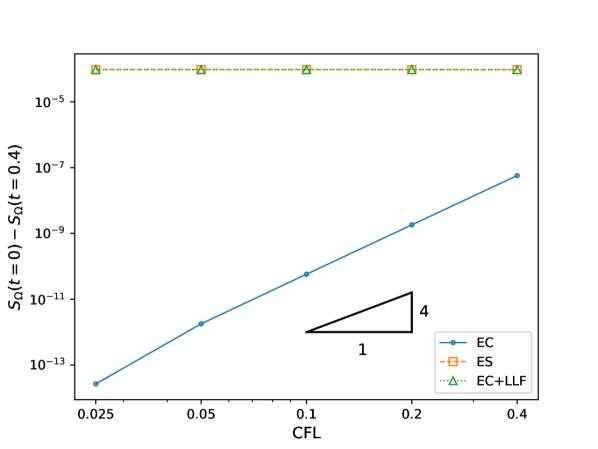
(a) Total entropy change

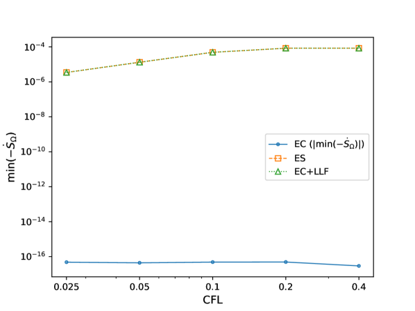
(b) Maximum entropy change rate

Figure 2: Log-log plots of the total entropy change and the maximum entropy change rate as a function of the CFL number for three different schemes: ((i) the entropy-conservative (EC) scheme, (ii) the provably entropy-stable scheme (ES), and (iii) the scheme that uses entropy-conservative fluxes in the volume integral together with the standard LLF scheme at the element interfaces (LLF).

Finally, Figure 2(b) presents the maximum rate of total entropy change observed across all time steps for each simulation, offering a detailed view of the schemes’ performance over time. This visualization confirms that both the ES scheme (ii) and the EC+LLF scheme (iii) consistently dissipate entropy throughout the simulation. A noteworthy observation is that the maximum rate of semi-discrete entropy dissipation for these schemes decreases with the reduction of the time-step size. This trend highlights the interplay between spatial and temporal discretization in influencing the schemes’ entropy characteristics. For clarity and to accommodate a logarithmic scale, we plot the absolute values of the maximum total entropy change rate for the entropy-conservative (EC) method (i), given that these values approach machine precision zero. This result shows that the EC scheme achieves ideal entropy conservation at the semi-discrete level, and it confirms that the net entropy dissipation illustrated in Figure 2(a) is a consequence of the time-integration scheme.

The results of this section support the mathematical analysis presented in Section 3.

4.3 Magnetized Kelvin-Helmholtz Instability

We consider a multi-ion extension of the magnetized Kelvin-Helmholtz instability problem proposed by Mignone et al. [4] to test the robustness of the scheme in turbulent under-resolved conditions.

We consider two ion species for this simulation: a hydrogen ion H⁺ ($k=1$) and an ionized hydrogen molecule H${}_{2}^{+}$ ($k=2)$. The heat capacity ratios are $\gamma_{1}=5/3$ and $\gamma_{2}=1.4$ for the monoatomic and diatomic molecules, respectively. Provided a suitable non-dimensionalization, the charge-to-mass ratios are $r_{1}=1$ and $r_{2}=1/2$. We do not consider collisional source terms between the ion species and assume a trivial electron pressure gradient, $\vec{\nabla}p_{e}=0$.

As in the single-species case, the initial condition is given by a shear layer with velocities in the $x$ direction, constant density and pressure, a small single-mode perturbation in the $y$-velocity, and a uniform magnetic field in the $xz$ plane. This initial condition evolves into a Kelvin-Helmholtz instability and breaks down into MHD turbulence. We set partial densities that sum up to unity, partial pressures that are computed with the individual heat capacity ratios, and the same velocities for the two ion species:

$$\rho_{k}(x,y,t=0) =\frac{1}{2}, p_{k}(x,y,t=0) =\frac{1}{\gamma_{k}}, {\color[rgb]{1,0,0}\psi(x,y,t=0)} {\color[rgb]{1,0,0}=0,}$$

$$v_{k,1}(x,y,t=0) =\frac{1}{2}\tanh\left(\frac{y}{y_{0}}\right), v_{k,2}(x,y,t=0) =v_{2,0}\sin(2\pi x)\exp\left(-\frac{y^{2}}{\sigma^{2}}\right), v_{k,3}(x,y,t=0) =0,$$

$$B_{1}(x,y,t=0) =c_{a}\cos\theta, B_{2}(x,y,t=0) =0, B_{3}(x,y,t=0) =c_{a}\sin\theta,$$ (86)

with $k=1,2$, $y_{0}=1/20$ is the steepness of the shear, $c_{a}=0.1$ is the Alfvén speed, and $\theta=\pi/3$ is the angle of the initial magnetic field. Moreover, the parameters of the perturbation are $v_{2,0}=0.01$ and $\sigma=0.1$.

We solve the multi-ion GLM-MHD system with the initial condition given by (4.3) in the domain $\Omega=[-1,1]^{2}$ with final time $t_{f}=20$, and the two dissipative solvers that we studied in Section 4.1: (ii) the provably entropy-stable (ES) scheme, and (iii) the EC+LLF scheme. The entropy-conserving (EC) scheme (i) does not provide enough dissipation to run this simulation stably. Moreover, we also test a standard LGL-DGSEM discretization of the multi-ion GLM-MHD equations that uses the standard LLF solver at the element interfaces. The standard LGL-DGSEM does not use a split formulation. For all simulations, we use a tessellation of $128\times 128$ quadrilateral elements of degree $N=3$, which corresponds to $512\times 512$ degrees of freedom (DOFs).

We would like to remark that the computational domain of the original study by Mignone et al. [4] spans $x\in[0,1]$, $y\in[-1,1]$, with periodic boundary conditions at the $x=0$ and $x=1$ boundaries, and perfectly conducting slip-wall boundary conditions at the $y=-1$ and $y=1$ boundaries. However, we use a square-shaped domain to accommodate this case to the two-dimensional TreeMesh solver of Trixi.jl. We use periodic boundary conditions at the $x=-1$ and $x=1$ boundaries, and perfectly conducting slip-wall boundary conditions at the $y=-1$ and $y=1$.

We impose the perfectly conducting slip-wall boundary condition weakly by evaluating the surface numerical flux and non-conservative terms with an outer state that mirrors the normal velocity and magnetic fields,

$$\mathbf{u}^{\mathrm{out}}(\mathbf{u}^{\mathrm{in}},\vec{n}) =\left(\rho^{\mathrm{out}}_{k},\rho^{\mathrm{out}}_{k}\vec{v}^{\mathrm{out}}_{k},E^{\mathrm{out}}_{k},\vec{B}^{\mathrm{out}},{\color[rgb]{1,0,0}\psi^{\mathrm{out}}}\right)^{T}$$

$$=\left(\rho^{\mathrm{in}}_{k},\rho^{\mathrm{in}}_{k}\left(\vec{v}^{\mathrm{in}}_{k}-2\vec{v}^{\mathrm{in}}_{k}\cdot\vec{n}\right),E^{\mathrm{in}}_{k},\vec{B}^{\mathrm{in}}-2\vec{B}^{\mathrm{in}}\cdot\vec{n},{\color[rgb]{1,0,0}\psi^{\mathrm{in}}}\right)^{T},$$ (87)

where $\vec{n}$ is the outward-pointing unit normal vector at the boundary of the domain. This simple way of prescribing the slip-wall boundary performs well in this particular example, as the main flow features develop away from the wall. In more challenging setups, it might be necessary to use a more robust slip-wall boundary condition. For instance, entropy-stable wall boundary conditions have been developed in [75, 76].

Figure 3 shows the evolution of the magnetized Kelvin-Helmholtz instability problem for the fourth-order ($N=3$) LGL-DGSEM that uses the provably entropy-stable (ES) solver (ii). We show the densities of species H⁺ and H${}_{2}^{+}$, and the ratio of the poloidal field,

$$B_{p}:=\sqrt{B_{1}^{2}+B_{2}^{2}},$$ (88)

to the toroidal field, $B_{t}:=B_{3}$. Even though we run the simulations on a square domain, $\Omega=[-1,1]^{2}$, we plot the quantities only for $x\in[0,1]$ to match the visualization presented in previous studies [4, 44], as the solution is periodic. At early stages of the simulation ($t\leq 5$), the perturbation follows a linear growth phase, in which the cat’s eye vortex structure forms, see e.g. the top row of Figure 3 and [4]. As the simulation continues, magnetic field lines become distorted and energy is transferred to smaller scales in the onset of MHD turbulence. Energy is then dissipated by the artificial viscosity and resistivity of the methods.

Figure 4 shows the evolution of the magnetized Kelvin-Helmholtz instability problem for the fourth-order ($N=3$) EC+LLF solver (iii): the LGL-DGSEM solver that uses the entropy-conserving flux in the volume integral and standard LLF fluxes at the element interfaces. Again, we show the densities of species H⁺ and H${}_{2}^{+}$, and the ratio of the poloidal to the toroidal magnetic field. The evolution of the two species’ densities and the magnetic field is almost identical as with the ES (ii) solver up to time $t=8$ (second panel). However, as turbulence evolves for later times of the simulation, the contours of Figure 4 differ from those in Figure 3. At those stages of the simulation, the evolution of the state quantities is determined by the slightly different (numerical) dissipation properties of the schemes (ii) and (iii).

	$\mathrm{H}^{+}$	$\mathrm{H}^{+}_{2}$

Figure 3: Evolution of the magnetized Kelvin-Helmholtz instability problem using a fourth-order ES discretization (ii) of the multi-ion MHD model at times $t=5$ (top panel), $t=8$ (second panel), $t=12$ (third panel) and $t=20$ (bottom panel) with the highest resolution ($256\times 512$ DOFs). We show the densities of the ion species, $H^{+}$ and $H^{+}_{2}$, and the ratio of the poloidal field, $B_{p}$, to the toroidal field, $B_{t}:=B_{3}$.

	$\mathrm{H}^{+}$	$\mathrm{H}^{+}_{2}$

Figure 4: Evolution of the magnetized Kelvin-Helmholtz instability problem using a fourth-order EC+LLF (iii) discretization of the multi-ion MHD model at times $t=5$ (top panel), $t=8$ (second panel), $t=12$ (third panel) and $t=20$ (bottom panel) with the highest resolution ($256\times 512$ DOFs). We show the densities of the ion species, $H^{+}$ and $H^{+}_{2}$, and the ratio of the poloidal field, $B_{p}$, to the toroidal field, $B_{t}:=B_{3}$.

Finally, Figure 5 shows the evolution of the $L_{2}$ norm of the normalized poloidal magnetic energy, defined as

$$\langle B_{p}^{2}\rangle(t):=\frac{\int_{\Omega}B_{p}^{2}(t)\mathrm{d}\vec{x}}{\int_{\Omega}B_{p}^{2}(t=0)\mathrm{d}\vec{x}},$$ (89)

and the $L_{2}$ norm of the divergence error. We show the solution obtained with five different methods/schemes (we use a numbering that is consistent with the numbering introduced in Section 4.1):

• ES: The provably entropy-stable split-form LGL-DGSEM discretization of the multi-ion GLM-MHD system (solid blue line).

• EC+LLF: The dissipative split-form LGL-DGSEM discretization of the multi-ion GLM-MHD system that uses the EC flux in the volume integral and the standard LLF flux at the element interfaces (dotted black line).

• ES (no GLM): The provably entropy-stable split-form LGL-DGSEM discretization (ii) without GLM divergence cleaning (dash-dot-dotted magenta line).

• EC+LLF (no GLM): The dissipative split-form LGL-DGSEM discretization (iii) without GLM divergence cleaning (dashed green line).

• Std DG: The standard LGL-DGSEM discretization of the multi-ion GLM-MHD system that does not use a split formulation and uses a standard LLF solver at the element interfaces (dash-dotted red line).

Only the solvers (ii) and (iii) are able to run the simulation until the end time, which highlights the importance of using the GLM divergence cleaning technique and an entropy-dissipative discretization. In accordance with the observations made for Figures 3 and 4, the evolution of the normalized poloidal magnetic energy and the divergence error is almost identical for the schemes (ii) and (iii) until time $t=9$. After that, the different dissipation properties of schemes (ii) and (iii) lead to slightly different results in the onset of MHD turbulence.

Figure 5(b) shows that schemes (iv) and (v) crash shortly after the formation of the cat’s eye vortex structure, as the divergence error grows uncontrollably due to the absence of the GLM divergence cleaning technique. The growth in the divergence error results in a non-physical evolution of the poloidal magnetic energy, as observed in Figure 5(a), and a flow in which a negative density/pressure causes the scheme to crash. Remarkably, the ES scheme without GLM (iv) manages to run for a little longer than the EC+LLF scheme (v).

Finally, it is noteworthy that the standard LGL-DGSEM discretization of the GLM-MHD system (vi) crashes when turbulence starts to develop in the domain. In other words, the GLM divergence cleaning technique is not enough to improve the robustness of the scheme. It is the combination of divergence cleaning and entropy stability that equips the LGL-DGSEM with enough robustness to run this example until the end time.

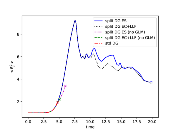
(a) Normalized poloidal magnetic energy

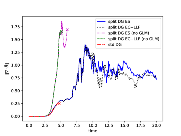
(b) Divergence error

Figure 5: Evolution of the normalized volume-integrated poloidal magnetic energy $\langle B_{p}^{2}\rangle$ and the $L_{2}$ norm of the divergence error $\left\lVert\vec{\nabla}\cdot\vec{B}\right\rVert$ for the magnetized KHI problem with two species (H⁺ and H${}_{2}^{+}$) and five different numerical schemes. An “x” marks the crash of a simulation.

5 Conclusions

This paper makes three significant contributions to the numerical analysis of the ideal multi-ion magneto-hydrodynamics (MHD) equations. Our first contribution involves enhancing the equation system with a divergence cleaning mechanism, utilizing the Generalized Lagrange Multiplier (GLM) technique. This addition ensures a more robust computational model by mitigating numerical divergence issues inherent in MHD simulations.

Our second contribution introduces an innovative algebraic manipulation of the system. This adjustment enables the identification of a strictly convex entropy function that aligns with the thermodynamic entropies of individual ion species. Consequently, our model adheres to the second law of thermodynamics at a continuous level, ensuring physical accuracy in simulations.

The third and final contribution of our work lies in the development of both finite volume (FV) and high-order discontinuous Galerkin (DG) entropy-consistent discretizations for the GLM-MHD system. These discretizations are notable for their entropy conservation or stability, aligning with the second law of thermodynamics at the semi-discrete level across any number of ion species. Moreover, they are consistent with established discretization schemes for single-fluid MHD equations when reduced to a single ion species scenario.

Through a series of numerical experiments, we validated the entropy-consistency, high-order accuracy, and improved robustness of our methods. These tests confirm the practical effectiveness and theoretical soundness of our contributions to the field of computational MHD.

The methods detailed in this paper are implemented for the two-dimensional Cartesian TreeMesh solver of the open-source framework Trixi.jl [68, 69, 67]. A reproducibility repository can be found on https://github.com/amrueda/paper_2024_multi-ion_mhd.

Appendices

Appendix A Derivation of the Entropy-Conservative Fluxes and Non-Conservative Terms

As reviewed in Section 3.1, numerical fluxes and non-conservative terms provide entropy conservation if they satisfy a generalization of Tadmor’s shuffle condition (50),

$$r_{(i,j)}=r(\mathbf{u}_{i},\mathbf{u}_{j})=\left\llbracket{\mathbf{w}}\right\rrbracket_{(i,j)}^{T}\hat{\mathbf{f}}_{(i,j)}^{{\mathrm{EC}}}+{\mathbf{w}}^{T}_{j}{\bm{\Phi}}^{\diamond{\mathrm{EC}}}_{(j,i)}-{\mathbf{w}}^{T}_{i}{\bm{\Phi}}^{\diamond{\mathrm{EC}}}_{(i,j)}-\left\llbracket\Psi\right\rrbracket_{(i,j)}=0,$$ (90)

where $r_{(i,j)}$ is the entropy production between degrees of freedom $i$ and $j$, and $\Psi$ is the so-called entropy (flux) potential, defined as (51)

$$\Psi={\mathbf{w}}^{T}\left(\mathbf{f}+\bm{\Phi}\right)-{f}^{S}=\underbrace{{\mathbf{w}}^{T}\mathbf{f}^{{\mathrm{Euler}}}-{f}^{S}}_{\coloneqq\Psi^{{\mathrm{Euler}}}}+\underbrace{{\mathbf{w}}^{T}\left(\mathbf{f}^{{\mathrm{mMHD}}}+\bm{\Phi}^{{\mathrm{mMHD}}}\right)}_{\coloneqq\Psi^{{\mathrm{mMHD}}}}+{\color[rgb]{1,0,0}\underbrace{{\mathbf{w}}^{T}\left(\mathbf{f}^{{\mathrm{GLM}}}+\bm{\Phi}^{{\mathrm{GLM}}}\right)}_{\coloneqq\Psi^{{\mathrm{GLM}}}}}.$$ (91)

Our approach to obtaining entropy-conservative two-point numerical fluxes and non-conservative terms involves breaking down the entropy-conserving flux into Euler, MHD and GLM components,

$$\hat{\mathbf{f}}^{{\mathrm{EC}}}_{(i,j)}=\hat{\mathbf{f}}^{{\mathrm{EC}},{\mathrm{Euler}}}_{(i,j)}+\hat{\mathbf{f}}^{{\mathrm{EC}},{\mathrm{mMHD}}}_{(i,j)}+{\color[rgb]{1,0,0}\hat{\mathbf{f}}^{{\mathrm{EC}},{\mathrm{GLM}}}_{(i,j)}},$$ (92)

and the entropy-conserving two-point non-conservative terms into Godunov-Powell, Lorentz, multi-ion, and GLM components,

$${\bm{\Phi}}^{\diamond{\mathrm{EC}}}_{(i,j)}={\bm{\Phi}}^{{\mathrm{GP}}\diamond,{\mathrm{EC}}}_{(i,j)}+{\bm{\Phi}}^{\rm{Lor}\diamond,{\mathrm{EC}}}_{(i,j)}+{\bm{\Phi}}^{\rm{multi}\diamond,{\mathrm{EC}}}_{(i,j)}+{\color[rgb]{1,0,0}{\bm{\Phi}}^{\rm{GLM}\diamond,{\mathrm{EC}}}_{(i,j)}}.$$ (93)

As discussed above, there are several solutions to (90), and we will focus on finding one consistent with the single-fluid GLM-MHD discretization of Derigs et al. [21]. The GLM terms are important to control the magnetic field divergence error and provide robustness to the schemes. However, all derivations of this paper are valid with or without GLM terms. Therefore, we mark all GLM terms in red to improve the readability.

We start by obtaining an entropy-conservative flux for the Euler terms. Since the Euler terms of each ion species of the multi-ion GLM-MHD system are completely decoupled from each other and correspond to individual copies of the Euler equations, it is straightforward to extend any existing entropy-conservative flux to these terms, e.g. [77, 48, 78]. In order to keep consistency with the EC flux of Derigs et al. [21] for single-fluid MHD, we choose the entropy-conserving and kinetic-energy preserving flux of Chandrashekar [77]. The multi-ion extension of this flux reads as

$$\mathbf{f}^{{\mathrm{EC}},{\mathrm{Euler}}}(\mathbf{u}_{L},\mathbf{u}_{R})=\begin{pmatrix}\rho^{\ln}_{k}\left\{\left\{v_{k,1}\right\}\right\}\\ \rho^{\ln}_{k}\left\{\left\{v_{k,1}\right\}\right\}^{2}+\overline{p}_{k}\\ \rho^{\ln}_{k}\left\{\left\{v_{k,1}\right\}\right\}\left\{\left\{v_{k,2}\right\}\right\}\\ \rho^{\ln}_{k}\left\{\left\{v_{k,1}\right\}\right\}\left\{\left\{v_{k,3}\right\}\right\}\\ f^{{\mathrm{EC}},{\mathrm{Euler}}}_{E_{k}}\\ \vec{0}\\ 0\end{pmatrix}$$ (94)

with

$$\begin{split}f^{{\mathrm{EC}},{\mathrm{Euler}}}_{E_{k}}=&f_{\rho_{k}}^{{\mathrm{EC}},{\mathrm{Euler}}}\bigg{[}\frac{1}{2(\gamma_{k}-1)\beta^{\ln}_{k}}-\frac{1}{2}\left(\left\{\left\{v_{k,1}^{2}\right\}\right\}+\left\{\left\{v_{k,2}^{2}\right\}\right\}+\left\{\left\{v_{k,3}^{2}\right\}\right\}\right)\bigg{]}\\ &+f_{\rho_{k}v_{k,1}}^{{\mathrm{EC}},{\mathrm{Euler}}}\left\{\left\{v_{k,1}\right\}\right\}+f_{\rho_{k}v_{k,2}}^{{\mathrm{EC}},{\mathrm{Euler}}}\left\{\left\{v_{k,2}\right\}\right\}+f_{\rho_{k}v_{k,3}}^{{\mathrm{EC}},{\mathrm{Euler}}}\left\{\left\{v_{k,3}\right\}\right\}\end{split}$$ (95)

and

$$\overline{p}_{k}=\frac{\left\{\left\{\rho_{k}\right\}\right\}}{2\left\{\left\{\beta_{k}\right\}\right\}}.$$

Following the derivations of Chandrashekar [77], it is possible to show that the flux (94) fulfills a conservative Tadmor shuffle condition in the multi-species sense, such that

$$\left\llbracket{\mathbf{w}}\right\rrbracket_{(i,j)}^{T}\hat{\mathbf{f}}_{(i,j)}^{{\mathrm{EC}},{\mathrm{Euler}}}=\left\llbracket\Psi^{{\mathrm{Euler}}}\right\rrbracket_{(i,j)}$$ (96)

holds. Hence, by substituting Equation (96) into Equation (90), it becomes evident that in order to achieve an entropy-conserving FV discretization of the multi-ion GLM-MHD system, it is sufficient to identify the MHD numerical fluxes and non-conservative terms that satisfy

$$\left\llbracket{\mathbf{w}}\right\rrbracket_{(i,j)}^{T}\hat{\mathbf{f}}_{(i,j)}^{{\mathrm{EC}},{\mathrm{mMHD}}}+{\mathbf{w}}^{T}_{j}{\bm{\Phi}}^{\diamond{\mathrm{EC}}}_{(j,i)}-{\mathbf{w}}^{T}_{i}{\bm{\Phi}}^{\diamond{\mathrm{EC}}}_{(i,j)}-\left\llbracket\Psi^{{\mathrm{mMHD}}}\right\rrbracket_{(i,j)}=0.$$ (97)

Contracting the local (non-conservative) part of the Godunov-Powell term yields

$${\mathbf{w}}^{T}\bm{\phi}^{{\mathrm{GP}}}= \left(\sum_{k}\frac{2r_{k}\rho_{k}\beta_{k}}{n_{e}e}\vec{v}_{k}\right)\cdot\vec{B}-\left(\sum_{k}2\beta_{k}\right)\vec{v}^{+}\cdot\vec{B}+2\beta_{+}\vec{v}^{+}\cdot\vec{B}$$

$$= 2\left(\sum_{k}\beta_{k}\vec{v}^{+}_{k}\right)\cdot\vec{B}.$$ (98)

Moreover, contracting the term $\bm{\Phi}^{\mathrm{Lor}}$ yields

$${\mathbf{w}}^{T}\bm{\Phi}^{\mathrm{Lor}}= \left[\sum_{k}2\beta_{k}\left(v^{+}_{k,1}\left(\frac{1}{2}\|\vec{B}\|^{2}+p_{e}\right)-\left(\vec{v}^{+}_{k}\cdot\vec{B}\right)B_{1}\right)\right]-2\left(\sum_{k}\beta_{k}v^{+}_{k,1}\right)p_{e}$$

$$= \left(\sum_{k}\beta_{k}v^{+}_{k,1}\right)\|\vec{B}\|^{2}-2\left(\sum_{k}\beta_{k}\vec{v}^{+}_{k}\right)\cdot\vec{B}B_{1}.$$ (99)

Since the multi-ion Godunov-Powell non-conservative term $\bm{\Upsilon}^{{\mathrm{GP}}}$ (43) is very similar to the single-species MHD Godunov-Powell term, we adopt the central discretization proposed by Winters and Gassner [62], and used in [22, 21, 41, 47, 44, 45], and extend it to the multi-ion framework. The Godunov-Powell numerical non-conservative term then reads as

$$\bm{\Phi}^{{\mathrm{GP}}\diamond,{\mathrm{EC}}}_{(i,j)}=\bm{\phi}^{{\mathrm{GP}}}_{i}\left\{\left\{B_{1}\right\}\right\}_{(i,j)},$$ (100)

which is consistent with the single-fluid GLM-MHD term.

We compute the contribution to the entropy production of the Godunov-Powell non-conservative term as

$${\mathbf{w}}_{j}^{T}\bm{\Phi}^{{\mathrm{GP}}\diamond,{\mathrm{EC}}}_{(j,i)}-{\mathbf{w}}_{i}^{T}\bm{\Phi}^{{\mathrm{GP}}\diamond,{\mathrm{EC}}}_{(i,j)}= 2\left\llbracket\left(\sum_{k}\beta_{k}\vec{v}^{+}_{k}\right)\cdot\vec{B}\right\rrbracket_{(i,j)}\left\{\left\{B_{1}\right\}\right\}_{(i,j)}$$

$$= {2\left(\sum_{k}\left\llbracket\beta_{k}\right\rrbracket_{(i,j)}\left\{\left\{\vec{v}^{+}_{k}\cdot\vec{B}\right\}\right\}_{(i,j)}\right)\left\{\left\{B_{1}\right\}\right\}_{(i,j)}}$$

$$+{2\left(\sum_{k}\left\{\left\{\beta_{k}\right\}\right\}_{(i,j)}\left\llbracket\vec{v}^{+}_{k}\cdot\vec{B}\right\rrbracket_{(i,j)}\right)\left\{\left\{B_{1}\right\}\right\}_{(i,j)}}$$ (101)

where we used the identity

$$\left\llbracket a\,b\right\rrbracket=\left\llbracket a\right\rrbracket\left\{\left\{b\right\}\right\}+\left\{\left\{a\right\}\right\}\left\llbracket b\right\rrbracket.$$ (102)

Finally, since the GLM terms contracted with the entropy variables read

$${\mathbf{w}}^{T}\left({\color[rgb]{1,0,0}\mathbf{f}^{\mathrm{GLM}}+\bm{\Phi}^{\mathrm{GLM}}}\right)=c_{h}\left(-2{\color[rgb]{1,0,0}\psi}B_{1}\sum_{k}\beta_{k}+2\beta_{+}B_{1}{\color[rgb]{1,0,0}\psi}+2{\color[rgb]{1,0,0}\psi}B_{1}\beta_{+}\right)-2\sum_{k}\beta_{k}v^{+}_{1}{\color[rgb]{1,0,0}\psi^{2}}+2\beta_{+}v^{+}_{1}{\color[rgb]{1,0,0}\psi^{2}}={\color[rgb]{1,0,0}2c_{h}\beta_{+}\psi B_{1}},$$ (103)

their contribution to the entropy flux potential is

$$\left\llbracket{\mathbf{w}}^{T}\left({\color[rgb]{1,0,0}\mathbf{f}^{\mathrm{GLM}}+\bm{\Phi}^{\mathrm{GLM}}}\right)\right\rrbracket={\color[rgb]{1,0,0}2c_{h}\left\llbracket\beta_{+}{\color[rgb]{1,0,0}\psi}B_{1}\right\rrbracket}.$$ (104)

We remark that there are different ways to apply the identity (102), which lead to slightly different terms. In this work, we follow the procedure detailed by Derigs et al. [21] and apply (102) to obtain terms that depend on the jumps of $\beta_{k}$, such that we can obtain discretizations consistent with Derigs et al.’s. By isolating the jump of other quantities, we would arrive at different (also valid) discretizations. For instance, if we applied the identity (102) to obtain terms that depend on the jumps of $\vec{B}$, we would obtain discretizations consistent with the single-fluid MHD fluxes of Chandrashekar and Klingenberg [22].

Note that $\bm{\Upsilon}^{\rm{Lor}}$ (44) is very similar to the single-fluid MHD magnetic flux. In fact, it contains the exact same momentum components of the single-fluid MHD magnetic flux, but it has a local non-conservative part and new terms containing the electron pressure. In the single-fluid MHD limit, the local non-conservative terms of the momentum equation become unity and the electron pressure is commonly assumed as negligible. To keep the consistency with the single-fluid GLM-MHD discretization of Derigs et al. [21], we adopt the momentum components of the single-species EC flux (used as well in [62, 22, 79]), and propose a consistent non-conservative FV discretization of the form

$$\bm{\Phi}^{\rm{Lor}\diamond,{\mathrm{EC}}}_{(i,j)}=\begin{pmatrix}0\\[2.84544pt] \frac{r_{k}\rho_{k}}{n_{e}e}\\[2.84544pt] \frac{r_{k}\rho_{k}}{n_{e}e}\\[2.84544pt] \frac{r_{k}\rho_{k}}{n_{e}e}\\[2.84544pt] v^{+}_{k,1}\\[2.84544pt] \vec{0}\\[2.84544pt] 0\end{pmatrix}_{i}\circ\begin{pmatrix}0\\[2.84544pt] \frac{1}{2}\left\{\left\{\|\vec{B}\|^{2}\right\}\right\}-\left\{\left\{B_{1}\right\}\right\}^{2}+\bar{p}_{e}\\[2.84544pt] -\left\{\left\{B_{1}\right\}\right\}\left\{\left\{B_{2}\right\}\right\}\\[2.84544pt] -\left\{\left\{B_{1}\right\}\right\}\left\{\left\{B_{3}\right\}\right\}\\[2.84544pt] \bar{p}_{e}\\[2.84544pt] \vec{0}\\[2.84544pt] 0\end{pmatrix}_{(i,j)},$$ (105)

with a yet to be determined symmetric “average” of the electron pressure $\bar{p}_{e}$.

Contracting $\bm{\Phi}^{\rm{Lor}\diamond,{\mathrm{EC}}}_{(i,j)}$ with the entropy variables reads

$${\mathbf{w}}_{i}^{T}\bm{\Phi}^{\rm{Lor}\diamond,{\mathrm{EC}}}_{(i,j)}= \left(\sum_{k}\beta_{k}v^{+}_{k,1}\right)_{i}\left(\left\{\left\{\|\vec{B}\|^{2}\right\}\right\}+2\bar{p}_{e}\right)-2\left(\sum_{k}\beta_{k}\vec{v}^{+}_{k}\right)_{i}\cdot\left\{\left\{\vec{B}\right\}\right\}\left\{\left\{B_{1}\right\}\right\}-2\left(\sum_{k}\beta_{k}v^{+}_{k,1}\right)_{i}\bar{p}_{e}$$

$$= \left(\sum_{k}\beta_{k}v^{+}_{k,1}\right)_{i}\left\{\left\{\|\vec{B}\|^{2}\right\}\right\}-2\left(\sum_{k}\beta_{k}\vec{v}^{+}_{k}\right)_{i}\cdot\left\{\left\{\vec{B}\right\}\right\}\left\{\left\{B_{1}\right\}\right\},$$ (106)

which shows that any consistent and symmetric “average” for the electron pressure can be used. For instance, we can use the simple average $\bar{p}_{e}=\left\{\left\{p_{e}\right\}\right\}$.

With the goal of being fully consistent with the single-species EC flux of Winters and Gassner [62] and Derigs et al. [21], but also with the multi-ion GLM-MHD source term, we propose a numerical MHD flux of the form

$$\hat{\mathbf{f}}^{{\mathrm{EC}},{\mathrm{mMHD}}}_{(i,j)}+{\color[rgb]{1,0,0}\hat{\mathbf{f}}^{{\mathrm{EC}},{\mathrm{GLM}}}_{(i,j)}}=\begin{pmatrix}0\\ \vec{0}\\ \hat{{f}}^{{\mathrm{EC}},{\mathrm{mMHD}}}_{E_{k},(i,j)}+{\color[rgb]{1,0,0}2c_{h}\left\{\left\{\psi\right\}\right\}\left\{\left\{B_{1}\right\}\right\}-c_{h}\left\{\left\{\psi B_{1}\right\}\right\}}\\ {\color[rgb]{1,0,0}c_{h}\left\{\left\{\psi\right\}\right\}}\\ \left\{\left\{v^{+}_{1}\right\}\right\}\left\{\left\{B_{2}\right\}\right\}-\left\{\left\{v^{+}_{2}\right\}\right\}\left\{\left\{B_{1}\right\}\right\}\\ \left\{\left\{v^{+}_{1}\right\}\right\}\left\{\left\{B_{3}\right\}\right\}-\left\{\left\{v^{+}_{3}\right\}\right\}\left\{\left\{B_{1}\right\}\right\}\\ {\color[rgb]{1,0,0}c_{h}\left\{\left\{B_{1}\right\}\right\}}\end{pmatrix},$$ (107)

and will solve for the unknown term $\hat{{f}}^{{\mathrm{EC}},{\mathrm{mMHD}}}_{E_{k},(i,j)}$.

The contraction of the term (107) with the jump of entropy variables reads

$$\left\llbracket{\mathbf{w}}^{T}\right\rrbracket_{(i,j)}\left(\hat{\mathbf{f}}^{{\mathrm{EC}},{\mathrm{mMHD}}}_{(i,j)}+{\color[rgb]{1,0,0}\hat{\mathbf{f}}^{{\mathrm{EC}},{\mathrm{GLM}}}_{(i,j)}}\right)= -2\sum_{k}\left\llbracket\beta_{k}\right\rrbracket\left(\hat{{f}}^{{\mathrm{EC}},{\mathrm{mMHD}}}_{E_{k},(i,j)}+{\color[rgb]{1,0,0}2c_{h}\left\{\left\{\psi\right\}\right\}\left\{\left\{B_{1}\right\}\right\}-c_{h}\left\{\left\{\psi B_{1}\right\}\right\}}\right)$$

$$+2\left\llbracket\beta^{+}B_{2}\right\rrbracket\left(\left\{\left\{v^{+}_{1}\right\}\right\}\left\{\left\{B_{2}\right\}\right\}-\left\{\left\{v^{+}_{2}\right\}\right\}\left\{\left\{B_{1}\right\}\right\}\right)$$

$$+2\left\llbracket\beta^{+}B_{3}\right\rrbracket\left(\left\{\left\{v^{+}_{1}\right\}\right\}\left\{\left\{B_{3}\right\}\right\}-\left\{\left\{v^{+}_{3}\right\}\right\}\left\{\left\{B_{1}\right\}\right\}\right)$$

$$+{\color[rgb]{1,0,0}2c_{h}\left\llbracket\beta_{+}B_{1}\right\rrbracket\left\{\left\{\psi\right\}\right\}+2c_{h}\left\llbracket\beta_{+}\psi\right\rrbracket\left\{\left\{B_{1}\right\}\right\}}$$

$$= -2\sum_{k}\left\llbracket\beta_{k}\right\rrbracket\hat{{f}}^{{\mathrm{EC}},{\mathrm{mMHD}}}_{E_{k},(i,j)}+2\left\llbracket\beta^{+}\vec{B}\right\rrbracket\cdot\left(\left\{\left\{\vec{B}\right\}\right\}\left\{\left\{v^{+}_{1}\right\}\right\}-\left\{\left\{\vec{v}^{+}\right\}\right\}\left\{\left\{B_{1}\right\}\right\}\right)$$

$$+{\color[rgb]{1,0,0}2c_{h}\left\llbracket\beta_{+}\psi B_{1}\right\rrbracket},$$ (108)

where the last GLM term is obtained using the identity (102) as follows:

$${\color[rgb]{1,0,0}-2\sum_{k}\left\llbracket\beta_{k}\right\rrbracket\left(2c_{h}\left\{\left\{\psi\right\}\right\}\left\{\left\{B_{1}\right\}\right\}-c_{h}\left\{\left\{\psi B_{1}\right\}\right\}\right)+2c_{h}\left\llbracket\beta_{+}B_{1}\right\rrbracket\left\{\left\{\psi\right\}\right\}+2c_{h}\left\llbracket\beta_{+}\psi\right\rrbracket\left\{\left\{B_{1}\right\}\right\}}$$

$$={\color[rgb]{1,0,0}-2\sum_{k}\left\llbracket\beta_{k}\right\rrbracket\left(2c_{h}\left\{\left\{\psi\right\}\right\}\left\{\left\{B_{1}\right\}\right\}-c_{h}\left\{\left\{\psi B_{1}\right\}\right\}\right)+2c_{h}\left(\sum_{k}\left\llbracket\beta_{k}B_{1}\right\rrbracket\left\{\left\{\psi\right\}\right\}+\left\llbracket\beta_{k}\psi\right\rrbracket\left\{\left\{B_{1}\right\}\right\}\right)}$$

$$={\color[rgb]{1,0,0}-2c_{h}\sum_{k}\left\llbracket\beta_{k}\right\rrbracket\left(2\left\{\left\{\psi\right\}\right\}\left\{\left\{B_{1}\right\}\right\}-\left\{\left\{\psi B_{1}\right\}\right\}\right)}$$

$$\quad\quad{\color[rgb]{1,0,0}+2c_{h}\left(\sum_{k}\left(\left\llbracket\beta_{k}\right\rrbracket\left\{\left\{B_{1}\right\}\right\}+\left\{\left\{\beta_{k}\right\}\right\}\left\llbracket B_{1}\right\rrbracket\right)\left\{\left\{\psi\right\}\right\}+\left(\left\llbracket\beta_{k}\right\rrbracket\left\{\left\{\psi\right\}\right\}+\left\{\left\{\beta_{k}\right\}\right\}\left\llbracket\psi\right\rrbracket\right)\left\{\left\{B_{1}\right\}\right\}\right)}$$

$$={\color[rgb]{1,0,0}-2c_{h}\sum_{k}\left\llbracket\beta_{k}\right\rrbracket\left(2\left\{\left\{\psi\right\}\right\}\left\{\left\{B_{1}\right\}\right\}-\left\{\left\{\psi B_{1}\right\}\right\}\right)+2c_{h}\left(\sum_{k}2\left\llbracket\beta_{k}\right\rrbracket\left\{\left\{B_{1}\right\}\right\}\left\{\left\{\psi\right\}\right\}+\left\{\left\{\beta_{k}\right\}\right\}\left\llbracket\psi B_{1}\right\rrbracket\right)}$$

$$={\color[rgb]{1,0,0}2c_{h}\sum_{k}\left\llbracket\beta_{k}\psi B_{1}\right\rrbracket=2c_{h}\left\llbracket\beta_{+}\psi B_{1}\right\rrbracket}.$$

Finally, taking into account that the non-conservative term $\bm{\Upsilon}^{\mathrm{multi}}$ (2.5) contains terms with the same structure as the induction equation terms of (107), we assume a numerical non-conservative term of the form

$$\bm{\Phi}^{\rm{multi}\diamond,{\mathrm{EC}}}_{(i,j)}= (B_{2})_{i}\begin{pmatrix}0\\ \vec{0}\\ \left\{\left\{v^{-}_{k,1}\right\}\right\}\left\{\left\{B_{2}\right\}\right\}-\left\{\left\{v^{-}_{k,2}\right\}\right\}\left\{\left\{B_{1}\right\}\right\}\\ \vec{0}\\ 0\end{pmatrix}+(B_{3})_{i}\begin{pmatrix}0\\ \vec{0}\\ \left\{\left\{v^{-}_{k,1}\right\}\right\}\left\{\left\{B_{3}\right\}\right\}-\left\{\left\{v^{-}_{k,3}\right\}\right\}\left\{\left\{B_{1}\right\}\right\}\\ \vec{0}\\ 0\end{pmatrix}$$

$$= \begin{pmatrix}0\\ \vec{0}\\ \vec{B}_{i}\cdot\left\{\left\{\vec{B}\right\}\right\}\left\{\left\{v^{-}_{k,1}\right\}\right\}-\vec{B}_{i}\cdot\left\{\left\{\vec{v}^{-}_{k}\right\}\right\}\left\{\left\{B_{1}\right\}\right\}\\ \vec{0}\\ 0\end{pmatrix}=\begin{pmatrix}0\\ \vec{0}\\ \vec{B}_{i}\cdot\vec{h}^{\rm{multi}*}_{E_{k},(i,j)}\\ \vec{0}\\ 0\end{pmatrix},$$ (109)

where we have introduced a new auxiliary quantity $\vec{h}^{\rm{multi}*}_{E_{k},(i,j)}$.

Contracting $\bm{\Phi}^{\rm{multi}\diamond,{\mathrm{EC}}}$ with the entropy variables reads

$${\mathbf{w}}_{i}^{T}\bm{\Phi}^{\rm{multi}\diamond,{\mathrm{EC}}}_{(i,j)}= -2\left(\sum_{k}\left(\beta_{k}\vec{B}\right)_{i}\left\{\left\{v^{-}_{k,1}\right\}\right\}\right)\cdot\left\{\left\{\vec{B}\right\}\right\}+2\left(\sum_{k}\left(\beta_{k}\vec{B}\right)_{i}\cdot\left\{\left\{\vec{v}^{-}_{k}\right\}\right\}\right)\left\{\left\{B_{1}\right\}\right\},$$ (110)

and therefore we have

$${\mathbf{w}}_{j}^{T}\bm{\Phi}^{\rm{multi}\diamond,{\mathrm{EC}}}_{(j,i)}-{\mathbf{w}}_{i}^{T}\bm{\Phi}^{\rm{multi}\diamond,{\mathrm{EC}}}_{(i,j)}= -2\left(\sum_{k}\left\llbracket\beta_{k}\vec{B}\right\rrbracket\left\{\left\{v^{-}_{k,1}\right\}\right\}\right)\cdot\left\{\left\{\vec{B}\right\}\right\}+2\left(\sum_{k}\left\llbracket\beta_{k}\vec{B}\right\rrbracket\cdot\left\{\left\{\vec{v}^{-}_{k}\right\}\right\}\right)\left\{\left\{B_{1}\right\}\right\}.$$ (111)

The next term contributing to the jump of the entropy potential is $\bm{\Phi}^{\rm{multi}}$. Its contraction with the entropy variables reads as

$${\mathbf{w}}^{T}\bm{\Phi}^{\rm{multi}}= -2\sum_{k}\beta_{k}\left(v^{-}_{k,1}B_{2}^{2}-v^{-}_{k,2}B_{1}B_{2}+v^{-}_{k,1}B_{3}^{2}-v^{-}_{k,3}B_{1}B_{3}\right)$$

$$= {-2\left(\sum_{k}\beta_{k}v^{-}_{k,1}\right)\|\vec{B}\|^{2}+2\left(\sum_{k}\beta_{k}\vec{v}^{-}_{k}\right)\cdot\vec{B}B_{1}}.$$ (112)

The contribution of the GLM terms to the EC-fluxes vanishes:

$${\mathbf{w}}^{T}_{i}{\color[rgb]{1,0,0}\bm{\Phi}^{\rm{GLM}\diamond,{\mathrm{EC}}}_{(i,j)}}={\color[rgb]{1,0,0}\left(-\sum_{k}2\beta_{k}v_{1}^{+}{\color[rgb]{1,0,0}\psi}+2\beta_{+}\psi v_{1}^{+}\right)_{i}{\color[rgb]{1,0,0}\left\{\left\{\psi\right\}\right\}}_{(i,j)}}=0,$$ (113)

and combining the GLM-terms in equations (A) and (104) yields a zero-sum of all GLM terms.

It remains only to compute the term $\hat{{f}}^{{\mathrm{EC}},{\mathrm{mMHD}}}_{E_{k},(i,j)}$. Following the procedure of Derigs et al. [21], we apply the identity (102) to all terms that contribute to (97), in order to obtain terms that depend on the jump of ${\beta_{k}}$. Now, we write only the terms that multiply $\left\llbracket\beta_{k}\right\rrbracket$ in (97):

• From $\left\llbracket{\mathbf{w}}\right\rrbracket^{T}\hat{\mathbf{f}}^{{\mathrm{EC}},{\mathrm{mMHD}}}_{(i,j)}$ (see (A)): $-2\hat{{f}}^{{\mathrm{EC}},{\mathrm{mMHD}}}_{E_{k},(i,j)}+2\left\{\left\{\vec{B}\right\}\right\}\cdot\vec{\hat{{f}}}^{{\mathrm{EC}},{\mathrm{mMHD}}}_{\vec{B},(i,j)}$

• From $\left\llbracket{\mathbf{w}}^{T}\left(\bm{\Phi}^{{\mathrm{GP}}}+\bm{\Phi}^{\mathrm{Lor}}\right)\right\rrbracket$ (see (A) and (A)): $\left\{\left\{v^{+}_{k,1}\|\vec{B}\|^{2}\right\}\right\}$

• From ${\mathbf{w}}_{j}^{T}\bm{\Phi}^{{\mathrm{GP}}\diamond,{\mathrm{EC}}}_{(j,i)}-{\mathbf{w}}_{i}^{T}\bm{\Phi}^{{\mathrm{GP}}\diamond,{\mathrm{EC}}}_{(i,j)}$ (see (A)): $2\left\{\left\{\vec{v}^{+}_{k}\cdot\vec{B}\right\}\right\}_{(i,j)}\left\{\left\{B_{1}\right\}\right\}_{(i,j)}$

• From ${\mathbf{w}}_{j}^{T}\bm{\Phi}^{\rm{Lor}\diamond,{\mathrm{EC}}}_{(j,i)}-{\mathbf{w}}_{i}^{T}\bm{\Phi}^{\rm{Lor}\diamond,{\mathrm{EC}}}_{(i,j)}$ (see (A)): $\left\{\left\{v^{+}_{k,1}\right\}\right\}\left\{\left\{\|\vec{B}\|^{2}\right\}\right\}-2\left\{\left\{\vec{v}^{+}_{k}\right\}\right\}\cdot\left\{\left\{\vec{B}\right\}\right\}\left\{\left\{B_{1}\right\}\right\}$

• From $\left\llbracket{\mathbf{w}}^{T}\bm{\Phi}^{\mathrm{multi}}\right\rrbracket$ (see (A)): $-2\left\{\left\{v^{-}_{k,1}\|\vec{B}\|^{2}\right\}\right\}+2\left\{\left\{\vec{v}^{-}_{k}\cdot\vec{B}B_{1}\right\}\right\}$

• From $\left\llbracket{\mathbf{w}}^{T}\mathbf{f}^{{\mathrm{mMHD}}}\right\rrbracket$ (see (42)): $-2\left\{\left\{v^{+}_{k,1}\|\vec{B}\|^{2}\right\}\right\}+2\left\{\left\{B_{1}\left(\vec{v}^{+}_{k}\cdot\vec{B}\right)\right\}\right\}+2\left\{\left\{v^{+}_{1}\|\vec{B}\|^{2}\right\}\right\}-2\left\{\left\{B_{1}\vec{v}^{+}\cdot\vec{B}\right\}\right\}$

• From ${\mathbf{w}}_{j}^{T}\bm{\Phi}^{\rm{multi}\diamond,{\mathrm{EC}}}_{(j,i)}-{\mathbf{w}}_{i}^{T}\bm{\Phi}^{\rm{multi}\diamond,{\mathrm{EC}}}_{(i,j)}$ (see (111)): $-2\left\{\left\{\vec{B}\right\}\right\}\cdot\vec{h}^{\rm{multi}*}_{E_{k},(i,j)}$

We obtain the entropy-conserving flux for the quantity $E_{k}$ by combining all terms into (97):

$$\hat{{f}}^{{\mathrm{EC}},{\mathrm{mMHD}}}_{E_{k},(i,j)}= \left\{\left\{\vec{B}\right\}\right\}\cdot\vec{\hat{{f}}}^{{\mathrm{EC}},{\mathrm{mMHD}}}_{\vec{B},(i,j)}-\frac{1}{2}\left\{\left\{v^{+}_{k,1}\|\vec{B}\|^{2}\right\}\right\}+\left\{\left\{\vec{v}^{+}_{k}\cdot\vec{B}\right\}\right\}_{(i,j)}\left\{\left\{B_{1}\right\}\right\}_{(i,j)}+\frac{1}{2}\left\{\left\{v^{+}_{k,1}\right\}\right\}\left\{\left\{\|\vec{B}\|^{2}\right\}\right\}$$

$$-\left\{\left\{\vec{v}^{+}_{k}\right\}\right\}\cdot\left\{\left\{\vec{B}\right\}\right\}\left\{\left\{B_{1}\right\}\right\}{\color[rgb]{0,1,0}+\left\{\left\{v^{-}_{k,1}\|\vec{B}\|^{2}\right\}\right\}-\left\{\left\{\vec{v}^{-}_{k}\cdot\vec{B}B_{1}\right\}\right\}}$$

$${\color[rgb]{0,1,0}+\left\{\left\{v^{+}_{k,1}\|\vec{B}\|^{2}\right\}\right\}-\left\{\left\{B_{1}\left(\vec{v}^{+}_{k}\cdot\vec{B}\right)\right\}\right\}-\left\{\left\{v^{+}_{1}\|\vec{B}\|^{2}\right\}\right\}+\left\{\left\{B_{1}\vec{v}^{+}\cdot\vec{B}\right\}\right\}}-\left\{\left\{\vec{B}\right\}\right\}\cdot\vec{h}^{\rm{multi}*}_{E_{k},(i,j)}$$

$$= \left\{\left\{\vec{B}\right\}\right\}\cdot\vec{\hat{{f}}}^{{\mathrm{EC}},{\mathrm{mMHD}}}_{\vec{B},(i,j)}-\frac{1}{2}\left\{\left\{v^{+}_{k,1}\|\vec{B}\|^{2}\right\}\right\}+\left\{\left\{\vec{v}^{+}_{k}\cdot\vec{B}\right\}\right\}_{(i,j)}\left\{\left\{B_{1}\right\}\right\}_{(i,j)}+\frac{1}{2}\left\{\left\{v^{+}_{k,1}\right\}\right\}\left\{\left\{\|\vec{B}\|^{2}\right\}\right\}$$

$$-\left\{\left\{\vec{v}^{+}_{k}\right\}\right\}\cdot\left\{\left\{\vec{B}\right\}\right\}\left\{\left\{B_{1}\right\}\right\}-\left\{\left\{\vec{B}\right\}\right\}\cdot\vec{h}^{\rm{multi}*}_{E_{k},(i,j)},$$ (114)

where the terms in green cancel each other out.

It is easy to see that, in the single-species case ($N_{i}=1$), the entropy-conserving flux (A) for the only ion species of the multi-ion GLM-MHD system is consistent with the EC flux for the energy term of Derigs et al. [21],

$$\hat{{f}}^{{\mathrm{EC}},\mathrm{MHD}}_{E,(i,j)}+{\color[rgb]{1,0,0}\hat{{f}}^{{\mathrm{EC}},\mathrm{GLM}}_{E,(i,j)}}= \left\{\left\{\vec{B}\right\}\right\}\cdot\vec{\hat{{f}}}^{{\mathrm{EC}},\mathrm{MHD}}_{\vec{B},(i,j)}-\frac{1}{2}\left\{\left\{v_{1}\|\vec{B}\|^{2}\right\}\right\}+\left\{\left\{\vec{v}\cdot\vec{B}\right\}\right\}_{(i,j)}\left\{\left\{B_{1}\right\}\right\}_{(i,j)}+\frac{1}{2}\left\{\left\{v_{1}\right\}\right\}\left\{\left\{\|\vec{B}\|^{2}\right\}\right\}$$

$$-\left\{\left\{\vec{v}\right\}\right\}\cdot\left\{\left\{\vec{B}\right\}\right\}\left\{\left\{B_{1}\right\}\right\}+{\color[rgb]{1,0,0}2c_{h}\left\{\left\{\psi\right\}\right\}\left\{\left\{B_{1}\right\}\right\}-c_{h}\left\{\left\{\psi B_{1}\right\}\right\}},$$ (115)

because in the single species case we have $\vec{v}=\vec{v}_{k}=\vec{v}^{+}_{k}$ and $\vec{v}^{-}_{k}=0$, and hence $\vec{\hat{{f}}}^{{\mathrm{EC}},{\mathrm{mMHD}}}_{\vec{B},(i,j)}=\vec{\hat{{f}}}^{{\mathrm{EC}},\mathrm{MHD}}_{\vec{B},(i,j)}$ and $\vec{h}^{\rm{multi}*}_{E_{k},(i,j)}=0$.

We can also check for consistency with the multi-ion GLM-MHD energy flux term (42). To do that, we evaluate the EC flux for the quantity $E_{k}$ (A) with the same left and right states:

$$\hat{{f}}^{{\mathrm{EC}},{\mathrm{mMHD}}}_{E_{k},(i,i)}+{\color[rgb]{1,0,0}\hat{{f}}^{{\mathrm{EC}},\rm{GLM}}_{E_{k},(i,i)}}= \vec{B}_{i}\cdot\vec{f}^{{\mathrm{mMHD}}}_{\vec{B},i}-\vec{B}_{i}\cdot\vec{h}^{\rm{multi}*}_{E_{k},(i,i)}+{\color[rgb]{1,0,0}c_{h}\left(\psi B_{1}\right)_{i}}$$

$$= \left[v^{+}_{1}\|\vec{B}\|^{2}-B_{1}\left(\vec{v}^{+}\cdot\vec{B}\right)\right]_{i}-\left[v^{-}_{k,1}\|\vec{B}\|^{2}-B_{1}\left(\vec{v}^{-}_{k}\cdot\vec{B}\right)\right]_{i}+{\color[rgb]{1,0,0}c_{h}\left(\psi B_{1}\right)_{i}}$$

$$= \left[v^{+}_{k,1}\|\vec{B}\|^{2}-B_{1}\left(\vec{v}^{+}_{k}\cdot\vec{B}\right)\right]_{i}+{\color[rgb]{1,0,0}c_{h}\left(\psi B_{1}\right)_{i}}$$

$$= f^{{\mathrm{mMHD}}}_{E_{k}}+{\color[rgb]{1,0,0}f^{\rm{GLM}}_{E_{k}}}.$$

References

- Toth et al. [2010] G. Toth, A. Glocer, Y. Ma, D. Najib, Multi-Ion Magnetohydrodynamics 429 (2010) 213–218.
- Stone et al. [2008] J. M. Stone, T. A. Gardiner, P. Teuben, J. F. Hawley, J. B. Simon, Athena: A New Code for Astrophysical MHD, The Astrophysical Journal Supplement Series 178 (2008) 137–177.
- Mignone et al. [2012] A. Mignone, C. Zanni, P. Tzeferacos, B. Van Straalen, P. Colella, G. Bodo, The PLUTO code for adaptive mesh computations in astrophysical fluid dynamics, Astrophysical Journal, Supplement Series 198 (2012).
- Mignone et al. [2010] A. Mignone, P. Tzeferacos, G. Bodo, High-order conservative finite difference GLM–MHD schemes for cell-centered MHD, Journal of Computational Physics 229 (2010) 5896–5920.
- Glocer et al. [2009] A. Glocer, G. Tóth, Y. Ma, T. Gombosi, J.-C. Zhang, L. Kistler, Multifluid block-adaptive-tree solar wind roe-type upwind scheme: Magnetospheric composition and dynamics during geomagnetic storms—initial results, Journal of Geophysical Research: Space Physics 114 (2009).
- Rubin et al. [2015] M. Rubin, X. Jia, K. Altwegg, M. Combi, L. Daldorff, T. Gombosi, K. Khurana, M. Kivelson, V. Tenishev, G. Tóth, et al., Self-consistent multifluid mhd simulations of europa’s exospheric interaction with jupiter’s magnetosphere, Journal of Geophysical Research: Space Physics 120 (2015) 3503–3524.
- Rubin et al. [2014] M. Rubin, M. Combi, L. Daldorff, T. Gombosi, K. Hansen, Y. Shou, V. Tenishev, G. Tóth, B. van der Holst, K. Altwegg, Comet 1p/halley multifluid mhd model for the giotto fly-by, The Astrophysical Journal 781 (2014) 86.
- Ghosh et al. [2019] D. Ghosh, T. D. Chapman, R. L. Berger, A. Dimits, J. Banks, A multispecies, multifluid model for laser–induced counterstreaming plasma simulations, Computers & Fluids 186 (2019) 38–57.
- Rambo and Procassini [1995] P. Rambo, R. Procassini, A comparison of kinetic and multifluid simulations of laser-produced colliding plasmas, Physics of Plasmas 2 (1995) 3130–3145.
- Munz et al. [2000] C. D. Munz, P. Omnes, R. Schneider, E. Sonnendrücker, U. Voß, Divergence Correction Techniques for Maxwell Solvers Based on a Hyperbolic Model, Journal of Computational Physics 161 (2000) 484–511.
- Dedner et al. [2002] A. Dedner, F. Kemm, D. Kröner, C. D. Munz, T. Schnitzer, M. Wesenberg, Hyperbolic divergence cleaning for the MHD equations, Journal of Computational Physics 175 (2002) 645–673.
- Balsara et al. [2021] D. S. Balsara, R. Kumar, P. Chandrashekar, Globally divergence-free dg scheme for ideal compressible mhd, Communications in Applied Mathematics and Computational Science 16 (2021) 59–98.
- Li and Shu [2005] F. Li, C.-W. Shu, Locally divergence-free discontinuous galerkin methods for mhd equations, Journal of Scientific Computing 22 (2005) 413–442.
- Balsara [2004] D. S. Balsara, Second-order-accurate schemes for magnetohydrodynamics with divergence-free reconstruction, The Astrophysical Journal Supplement Series 151 (2004) 149.
- Fey and Torrilhon [2003] M. Fey, M. Torrilhon, A constrained transport upwind scheme for divergence-free advection, in: Hyperbolic problems: theory, numerics, applications, Springer, 2003, pp. 529–538.
- Balsara and Dumbser [2015] D. S. Balsara, M. Dumbser, Divergence-free mhd on unstructured meshes using high order finite volume schemes based on multidimensional riemann solvers, Journal of Computational Physics 299 (2015) 687–715.
- Balsara et al. [2009] D. S. Balsara, T. Rumpf, M. Dumbser, C.-D. Munz, Efficient, high accuracy ader-weno schemes for hydrodynamics and divergence-free magnetohydrodynamics, Journal of Computational Physics 228 (2009) 2480–2516.
- Godunov [1972] S. K. Godunov, Symmetric form of the equations of magnetohydrodynamics, Numerical Methods for Mechanics of Continuum Medium 1 (1972) 26–34.
- Powell [1994] K. G. Powell, An approximate Riemann solver for magnetohydrodynamics (that works in more than one dimension), Technical Report, 1994.
- Powell et al. [1999] K. G. Powell, P. L. Roe, T. J. Linde, T. I. Gombosi, D. L. De Zeeuw, A solution-adaptive upwind scheme for ideal magnetohydrodynamics, Journal of Computational Physics 154 (1999) 284–309.
- Derigs et al. [2018] D. Derigs, A. R. Winters, G. J. Gassner, S. Walch, M. Bohm, Ideal GLM-MHD: About the entropy consistent nine-wave magnetic field divergence diminishing ideal magnetohydrodynamics equations, Journal of Computational Physics 364 (2018) 420–467.
- Chandrashekar and Klingenberg [2016] P. Chandrashekar, C. Klingenberg, Entropy stable finite volume scheme for ideal compressible MHD on 2-D Cartesian meshes, SIAM Journal on Numerical Analysis 54 (2016) 1313–1340.
- Wang et al. [2013] Z. J. Wang, K. Fidkowski, R. Abgrall, F. Bassi, D. Caraeni, A. Cary, H. Deconinck, R. Hartmann, K. Hillewaert, H. T. Huynh, N. Kroll, G. May, P.-O. Persson, B. van Leer, M. Visbal, B. van Leer, M. Visbal, High-order CFD methods: current status and perspective, International Journal for Numerical Methods in Fluids 72 (2013) 811–845.
- Cockburn et al. [2000] B. Cockburn, G. E. Karniadakis, C.-W. Shu, The Development of Discontinuous Galerkin Methods, Discontinuous Galerkin Methods 11 (2000) 3–50.
- Hindenlang et al. [2012] F. Hindenlang, G. J. Gassner, C. Altmann, A. Beck, M. Staudenmaier, C. D. Munz, Explicit discontinuous Galerkin methods for unsteady problems, Computers and Fluids 61 (2012) 86–93.
- Krais et al. [2021] N. Krais, A. Beck, T. Bolemann, H. Frank, D. Flad, G. Gassner, F. Hindenlang, M. Hoffmann, T. Kuhn, M. Sonntag, C. D. Munz, FLEXI: A high order discontinuous Galerkin framework for hyperbolic–parabolic conservation laws, Computers and Mathematics with Applications 81 (2021) 186–219.
- Ferrer et al. [2023] E. Ferrer, G. Rubio, G. Ntoukas, W. Laskowski, O. Mariño, S. Colombo, A. Mateo-Gabín, H. Marbona, F. M. de Lara, D. Huergo, et al., Horses3d: A high-order discontinuous galerkin solver for flow simulations and multi-physics applications, Computer Physics Communications 287 (2023) 108700.
- Fisher et al. [2013] T. C. Fisher, M. H. Carpenter, J. Nordström, N. K. Yamaleev, C. Swanson, Discretely conservative finite-difference formulations for nonlinear conservation laws in split form: Theory and boundary conditions, Journal of Computational Physics 234 (2013) 353–375.
- Gassner [2013] G. J. Gassner, A Skew-Symmetric Discontinuous Galerkin Spectral Element Discretization and Its Relation to SBP-SAT Finite Difference Methods, SIAM Journal on Scientific Computing 35 (2013) A1233–A1253.
- Carpenter et al. [2014] M. H. Carpenter, T. C. Fisher, E. J. Nielsen, S. H. Frankel, Entropy stable spectral collocation schemes for the Navier-Stokes Equations: Discontinuous interfaces, SIAM Journal on Scientific Computing 36 (2014) B835–B867.
- Svärd and Nordström [2014] M. Svärd, J. Nordström, Review of summation-by-parts schemes for initial-boundary-value problems, Journal of Computational Physics 268 (2014) 17–38.
- Fernández et al. [2014] D. C. D. R. Fernández, J. E. Hicken, D. W. Zingg, Review of summation-by-parts operators with simultaneous approximation terms for the numerical solution of partial differential equations, Computers & Fluids 95 (2014) 171–196.
- Fisher and Carpenter [2013] T. C. Fisher, M. H. Carpenter, High-order entropy stable finite difference schemes for nonlinear conservation laws: Finite domains, Journal of Computational Physics 252 (2013) 518–557.
- Gassner et al. [2016] G. J. Gassner, A. R. Winters, D. A. Kopriva, Split form nodal discontinuous Galerkin schemes with summation-by-parts property for the compressible Euler equations, Journal of Computational Physics 327 (2016) 39–66.
- Wintermeyer et al. [2017] N. Wintermeyer, A. R. Winters, G. J. Gassner, D. A. Kopriva, An entropy stable nodal discontinuous Galerkin method for the two dimensional shallow water equations on unstructured curvilinear meshes with discontinuous bathymetry, Journal of Computational Physics 340 (2017) 200–242.
- Manzanero et al. [2020] J. Manzanero, G. Rubio, D. A. Kopriva, E. Ferrer, E. Valero, An entropy–stable discontinuous Galerkin approximation for the incompressible navier–stokes equations with variable density and artificial compressibility, Journal of Computational Physics 408 (2020) 109241.
- Gassner et al. [2018] G. J. Gassner, A. R. Winters, F. J. Hindenlang, D. A. Kopriva, The BR1 scheme is stable for the compressible Navier–Stokes equations, Journal of Scientific Computing 77 (2018) 154–200.
- Renac [2019] F. Renac, Entropy stable DGSEM for nonlinear hyperbolic systems in nonconservative form with application to two-phase flows, Journal of Computational Physics 382 (2019) 1–26.
- Manzanero et al. [2020] J. Manzanero, G. Rubio, D. A. Kopriva, E. Ferrer, E. Valero, Entropy–stable discontinuous Galerkin approximation with summation–by–parts property for the incompressible navier–stokes/cahn–hilliard system, Journal of Computational Physics 408 (2020) 109363.
- Coquel et al. [2021] F. Coquel, C. Marmignon, P. Rai, F. Renac, An entropy stable high-order discontinuous galerkin spectral element method for the baer-nunziato two-phase flow model, Journal of Computational Physics 431 (2021) 110135.
- Bohm et al. [2018] M. Bohm, A. R. Winters, G. J. Gassner, D. Derigs, F. Hindenlang, J. Saur, An entropy stable nodal discontinuous Galerkin method for the resistive MHD equations. Part I: Theory and numerical verification, Journal of Computational Physics 1 (2018) 1–35.
- Black [1999] K. Black, A conservative spectral element method for the approximation of compressible fluid flow, Kybernetika 35 (1999) 133–146.
- Kopriva [2009] D. A. Kopriva, Implementing spectral methods for partial differential equations: Algorithms for scientists and engineers, Springer Science & Business Media, 2009.
- Rueda-Ramírez et al. [2023] A. M. Rueda-Ramírez, F. J. Hindenlang, J. Chan, G. J. Gassner, Entropy-stable gauss collocation methods for ideal magneto-hydrodynamics, Journal of Computational Physics 475 (2023) 111851.
- Rueda-Ramírez and Gassner [2024] A. M. Rueda-Ramírez, G. J. Gassner, A flux-differencing formula for split-form summation by parts discretizations of non-conservative systems: Applications to subcell limiting for magneto-hydrodynamics, Journal of Computational Physics 496 (2024) 112607.
- Rueda-Ramírez et al. [2020] A. M. Rueda-Ramírez, E. Ferrer, D. A. Kopriva, G. Rubio, E. Valero, A statically condensed discontinuous Galerkin spectral element method on Gauss-Lobatto nodes for the compressible Navier-Stokes equations, Journal of Computational Physics (2020).
- Rueda-Ramírez et al. [2021] A. M. Rueda-Ramírez, S. Hennemann, F. J. Hindenlang, A. R. Winters, G. J. Gassner, An entropy stable nodal discontinuous galerkin method for the resistive mhd equations. part ii: Subcell finite volume shock capturing, Journal of Computational Physics 444 (2021) 110580.
- Ismail and Roe [2009] F. Ismail, P. L. Roe, Affordable, entropy-consistent Euler flux functions II: Entropy production at shocks, Journal of Computational Physics 228 (2009) 5410–5436.
- Godlewski et al. [1998] E. Godlewski, P.-A. Raviart, R. J. LeVeque, Numerical approximation of hyperbolic systems of conservation laws, SIAM Review 40 (1998) 160–161.
- Barth [1999] T. J. Barth, Numerical methods for gasdynamic systems on unstructured meshes, in: An introduction to recent developments in theory and numerics for conservation laws, Springer, 1999, pp. 195–285.
- Hantke and Müller [2018] M. Hantke, S. Müller, Analysis and simulation of a new multi-component two-phase flow model with phase transitions and chemical reactions, Quarterly of applied mathematics 76 (2018) 253–287.
- Chan et al. [2019] J. Chan, D. C. D. R. Fernandez, M. H. Carpenter, D. C. Del Rey Fernández, M. H. Carpenter, Efficient entropy stable Gauss collocation methods, SIAM Journal on Scientific Computing 41 (2019) A2938—-A2966.
- Chan and Wilcox [2019] J. Chan, L. C. Wilcox, On discretely entropy stable weight-adjusted discontinuous Galerkin methods: curvilinear meshes, Journal of Computational Physics 378 (2019) 366–393.
- Derigs et al. [2017] D. Derigs, A. R. Winters, G. J. Gassner, S. Walch, A novel averaging technique for discrete entropy-stable dissipation operators for ideal MHD, Journal of Computational Physics 330 (2017) 624–632.
- Boyd and Vandenberghe [2004] S. P. Boyd, L. Vandenberghe, Convex optimization, Cambridge university press, 2004.
- Rueda-Ramírez and Gassner [2021] A. M. Rueda-Ramírez, G. J. Gassner, A Subcell Finite Volume Positivity-Preserving Limiter for DGSEM Discretizations of the Euler Equations, in: WCCM-ECCOMAS2020, pp. 1–12.
- Tadmor [1987] E. Tadmor, Entropy functions for symmetric systems of conservation laws, Journal of Mathematical Analysis and Applications 122 (1987) 355–359.
- Tadmor [1986] E. Tadmor, A minimum entropy principle in the gas dynamics equations, Applied Numerical Mathematics 2 (1986) 211–219.
- Tadmor [2003] E. Tadmor, Entropy stability theory for difference approximations of nonlinear conservation laws and related time-dependent problems, Acta Numerica 12 (2003) 451–512.
- Manzanero [2020] J. Manzanero, A high-order discontinuous Galerkin multiphase flow solver for industrial applications, Ph.D. thesis, Universidad Politécnica de Madrid, 2020.
- Fjordholm et al. [2012] U. S. Fjordholm, S. Mishra, E. Tadmor, Arbitrarily high-order accurate entropy stable essentially nonoscillatory schemes for systems of conservation laws, SIAM Journal on Numerical Analysis 50 (2012) 544–573.
- Winters and Gassner [2016] A. R. Winters, G. J. Gassner, Affordable, entropy conserving and entropy stable flux functions for the ideal MHD equations, Journal of Computational Physics 304 (2016) 72–108.
- Duan and Tang [2021] J. Duan, H. Tang, High-order accurate entropy stable finite difference schemes for the shallow water magnetohydrodynamics, Journal of Computational Physics 431 (2021) 110136.
- Duan and Tang [2019] J. Duan, H. Tang, High-order accurate entropy stable finite difference schemes for one-and two-dimensional special relativistic hydrodynamics, arXiv preprint arXiv:1905.06092 (2019).
- Tóth et al. [2021] G. Tóth, Y. Chen, Z. Huang, B. van der Holst, Challenges in modeling the outer magnetosphere, Magnetospheres in the Solar System (2021) 715–728.
- Carpenter and Kennedy [1994] M. H. Carpenter, C. A. Kennedy, Fourth-order 2N-storage Runge-Kutta schemes, Technical Report, 1994.
- Schlottke-Lakemper et al. [2021a] M. Schlottke-Lakemper, A. R. Winters, H. Ranocha, G. J. Gassner, A purely hyperbolic discontinuous galerkin approach for self-gravitating gas dynamics, Journal of Computational Physics 442 (2021a) 110467.
- Schlottke-Lakemper et al. [2021b] M. Schlottke-Lakemper, G. J. Gassner, H. Ranocha, A. R. Winters, J. Chan, Trixi.jl: Adaptive high-order numerical simulations of hyperbolic PDEs in Julia, https://github.com/trixi-framework/Trixi.jl, 2021b.
- Ranocha et al. [2022] H. Ranocha, M. Schlottke-Lakemper, A. R. Winters, E. Faulhaber, J. Chan, G. Gassner, Adaptive numerical simulations with Trixi.jl: A case study of Julia for scientific computing, Proceedings of the JuliaCon Conferences 1 (2022) 77.
- Najib et al. [2011] D. Najib, A. F. Nagy, G. Tóth, Y. Ma, Three-dimensional, multifluid, high spatial resolution mhd model studies of the solar wind interaction with mars, Journal of Geophysical Research: Space Physics 116 (2011).
- Maxima [2023] Maxima, Maxima, a computer algebra system. version 5.47.0, 2023.
- Hindenlang and Gassner [2020] F. J. Hindenlang, G. J. Gassner, On the order reduction of entropy stable dgsem for the compressible euler equations, in: Spectral and High Order Methods for Partial Differential Equations ICOSAHOM 2018: Selected Papers from the ICOSAHOM Conference, London, UK, July 9-13, 2018, Springer International Publishing, pp. 21–44.
- Hennemann et al. [2020] S. Hennemann, A. M. Rueda-Ramírez, F. J. Hindenlang, G. J. Gassner, A provably entropy stable subcell shock capturing approach for high order split form DG for the compressible Euler equations, Journal of Computational Physics (2020) 109935.
- Czernik [2022] C. Czernik, Entropy Stable Discontinuous Galerkin Methods for Multi-Component Euler and Ideal Magnetohydrodynamics Equations with Chemical Networks in Julia, Ph.D. thesis, Universität zu Köln, 2022.
- Hindenlang et al. [2020] F. J. Hindenlang, G. J. Gassner, D. A. Kopriva, Stability of wall boundary condition procedures for discontinuous galerkin spectral element approximations of the compressible euler equations, Spectral and High Order Methods for Partial Differential Equations 3 (2020).
- Chan et al. [2022] J. Chan, Y. Lin, T. Warburton, Entropy stable modal discontinuous galerkin schemes and wall boundary conditions for the compressible navier-stokes equations, Journal of Computational Physics 448 (2022) 110723.
- Chandrashekar [2013] P. Chandrashekar, Kinetic energy preserving and entropy stable finite volume schemes for compressible euler and navier-stokes equations, Communications in Computational Physics 14 (2013) 1252–1286.
- Ranocha et al. [2020] H. Ranocha, L. Dalcin, M. Parsani, Fully discrete explicit locally entropy-stable schemes for the compressible Euler and Navier–Stokes equations, Computers and Mathematics with Applications 80 (2020) 1343–1359.
- Winters et al. [2017] A. R. Winters, D. Derigs, G. J. Gassner, S. Walch, A uniquely defined entropy stable matrix dissipation operator for high Mach number ideal MHD and compressible Euler simulations, Journal of Computational Physics 332 (2017) 274–289.