Fast and Efficient Sequential Radar Parameter
Estimation in MIMO-OTFS Systems

Abstract

We consider the estimation of three-dimensional (3D) radar parameters, namely, bearing or angle-of-arrival (AoA), delay or range, and Doppler shift velocity, under a mono-static multiple-input multiple-output (MIMO) joint communications and radar (JCR) system based on Orthogonal Time Frequency Space (OTFS) signals. In particular, we propose a novel two-step algorithm to estimate the three radar parameters sequentially, where the AoA is obtained first, followed by the estimation of range and velocity via a reduced two-dimensional (2D) grid maximum likelihood (ML) search in the delay-Doppler (DD) domain. Besides the resulting lower complexity, the decoupling of AoA and DD estimation enables the incorporation of an linear minimum mean square error (LMMSE) procedure in the ML estimation of range and velocity, which are found to significantly outperform State-of-the-Art (SotA) alternatives and approach the fundamental limits of the Cramèr-Rao lower bound (CRLB) and search grid resolution.

Index Terms—  JCR, OTFS, MIMO, AoA, DD, LMMSE, Root multiple signal classification (MUSIC), low-complexity.

1 Introduction

Besides its inherent robustness to mobility, Orthogonal Time Frequency Space (OTFS) [1] has received great attention since its inception due to its ability to enable both communication and radar sensing applications [2, 3, 4, 5, 6], via the exploitation of its delay-Doppler (DD) channel structure.

Various radar techniques have been proposed to extract target information (delay and Doppler parameters) under single-input single-output (SISO) set-ups. One of the first attempts in [2], utilizes a simple matched-filter (MF)-based approach to detect a single target. Later, other methods considering more realistic scenarios were proposed [3], where a maximum likelihood (ML)-based method was used to iteratively estimate both delay and Doppler parameters in a multi-target situation.

It was identified, however, that the complexity of the ML-based methods is prohibitive, especially with high precision [6], since a full grid-search is required across the vicinity of the DD plane. This is further exacerbated when evolving from SISO to multiple-input multiple-output (MIMO) radar systems, which is considered a key technology for joint communications and sensing (JCAS), due to its ability to distinguish multiple targets via the additional spatial dimension [7], whose diversity is exploited in communication systems to improve the performance and robustness of modulation schemes.

Coupled with beamforming (BF) design and the calibration of co-located transmit and receive antenna arrays, MIMO radar is an extremely effective way to cover large angular sectors for target detection and radar parameter estimation. The performance gains of MIMO-OTFS systems come, however, at the price of a third signal domain – namely, the angle-of-arrival (AoA) domain – such that the radar parameter becomes a three-dimensional (3D) search problem of overwhelming complexity, as discussed in [4].

In light of the above, we contribute to improving the performance of 3D radar parameter estimation using MIMO-OTFS signals, with a reduction of complexity as a bonus. To that end, a novel two-step algorithm is proposed whereby AoA and DD estimation are decoupled, such that in addition to essentially converting the original 3D MIMO-OTFS problem to two-dimensional (2D) search of complexity comparable to that of the earlier SISO case [6], the incorporation of a linear minimum mean square error (LMMSE) procedure into the formulation of the DD search is enabled, resulting in substantial gains in performance.

$$\mathbf{h}_{n,m}[n^{\prime},m^{\prime}]=\sum_{p=1}^{P}h^{\prime}_{p}\cdot\mathbf{b}(\phi_{p})\mathbf{a}^{\mathsf{H}}(\phi_{p})\mathbf{f}_{\mathrm{BF}}\cdot C_{g_{\text{tx}},g_{\text{rx}}}\big{(}(n-n^{\prime})T-\tau_{p},(m-m^{\prime})\Delta f-\nu_{p}\big{)}\cdot e^{j2\pi n^{\prime}T\nu_{p}}\cdot e^{j2\pi m\Delta f\tau_{p}}\in\mathbb{C}\vspace{-1ex}$$ (8)
$${\varPsi}^{p}_{k,k^{\prime}}[\ell,\ell^{\prime}]\approx\frac{1}{NM}\cdot\frac{1-e^{j2\pi(k^{\prime}-k+\nu_{p}NT)}}{1-e^{j2\pi\frac{(k^{\prime}-k+\nu_{p}NT)}{N}}}\cdot\frac{1-e^{j2\pi(\ell^{\prime}-\ell+\tau_{p}M\Delta f)}}{1-e^{j2\pi\frac{(\ell^{\prime}-\ell+\tau_{p}M\Delta f)}{M}}}e^{-j2\pi\nu_{p}\frac{\ell^{\prime}}{M\Delta f}}\begin{cases}1,&\text{if }\ell^{\prime}\in\mathcal{L}_{ICI}\\ e^{-j2\pi(\frac{k^{\prime}}{N}+\nu_{p}T)},&\text{if }\ell^{\prime}\in\mathcal{L}_{ISI}\end{cases}$$ (11)

2 System Model

2.1 MIMO-OTFS Channel Model

Consider a uniform linear array (ULA) MIMO radar equipped with $N_{\mathrm{a}}$ antennas, operating in full-duplex mode as in [4], at a carrier frequency of $f_{\mathrm{c}}\;\mathrm{Hz}$ with channel bandwidth $B\;\mathrm{Hz}$.

It is assumed that a point target model is adopted for the system, such that each target can be modeled through its line-of-sight (LoS) path only [8] and thus represented by a unique single tap in the DD channel corresponding to the round-trip of the signal. Then, the corresponding time-frequency selective OTFS channel with $P$ taps [4, 9] can be described as

$$\!\mathbf{H}(t,\tau)\!=\!\!\sum_{p=1}^{P}h_{p}\!\cdot\!\delta(\tau\!-\!\tau_{p})\!\cdot\!e^{j2\pi\nu_{p}t}\!\cdot\!\mathbf{b}(\!\phi_{p}\!)\mathbf{a}^{\mathsf{H}}(\!\phi_{p}\!)\in\mathbb{C}^{N_{a}\times N_{a}}\!,\!\!\!\!\!$$ (1)

where $h_{p}\in\mathbb{C}$ with $p\in\{1,\cdots,P\}$ is the complex channel gain including the pathloss component; $\tau_{p}$ and $\nu_{p}$ are the round-trip delay and Doppler-shift of the $p$-th target given by

$$\tau_{p}\triangleq\frac{2r_{p}}{c}\in\mathbb{R},~{}~{}\text{and}~{}~{}\nu_{p}\triangleq\frac{2v_{p}f_{\mathrm{c}}}{c}\in\mathbb{R},$$ (2)

with $r_{p}\in\mathbb{R}$, $v_{p}\in\mathbb{R}$ denoting the range and velocities of the $p$-th target, respectively, and $c$ denoting the velocity of light at $299,792,458\;\mathrm{m/s}$; $\phi_{p}\in[-\frac{\pi}{2},\frac{\pi}{2}]$ is the ULA steering angle of the $p$-th target; and $\mathbf{a}(\phi)=[a_{1}(\phi),\cdots,a_{N_{\mathrm{a}}}\!(\phi)]^{\mathsf{T}}$ $\in$ $\mathbb{C}^{N_{\mathrm{a}}\times 1}$ and $\mathbf{b}(\phi)=[b_{1}(\phi),\cdots,b_{N_{\mathrm{a}}}\!(\phi)]^{\mathsf{T}}$ $\in$ $\mathbb{C}^{N_{\mathrm{a}}\times 1}$ are respectively the transmit and receive steering vectors with elements

$$a_{n}(\phi)=b_{n}(\phi)=e^{j(n-1)\pi\sin(\phi)}\in\mathbb{C}.$$ (3)

2.2 OTFS Transmit Signal Model

The OTFS signal structure considered is classic [4, 3], with $M$ subcarriers of bandwidth $\Delta f\triangleq B/M$, each conveying $N$ modulated symbols taken from an arbitrary quadrature amplitude modulation (QAM) constellation $\mathcal{X}$ with symbol duration $T\triangleq 1/{\Delta f}$, such that the total OTFS frame duration is $NT$.

In other words, the modulated symbols $x_{k,\ell}\in\mathbb{C}$, represented by the DD domain symbol matrix $\mathbf{X}\in\mathbb{C}^{N\times M}$, with $k\in\{0,\cdots,N-1\}$ and $\ell\in\{0,\cdots,M-1\}$, are arranged in the DD domain grid $\Gamma$, with a corresponding delay of $k/NT$ seconds and a Doppler of $\ell/M\Delta f$ $\mathrm{Hz}$. The transmitter performs the inverse symplectic finite Fourier transform (ISFFT) on the DD grid to convert the data into the dual (time-frequency) domain, whose samples are given by

$$X[n,m]=\sum_{k=0}^{N-1}\sum_{l=0}^{M-1}x_{k,\ell}\cdot e^{j2\pi(\frac{nk}{N}-\frac{m\ell}{M})}\in\mathbb{C},\vspace{-1ex}$$ (4)

with $n=\{0,\dots,N-1\}$ and $m=\{0,\dots,M-1\}$, obeying the average power constraint $\mathbb{E}[|X[n,m]|^{2}]\leq P_{\text{avg}}/N_{a}$.

Utilizing the time-frequency data samples $X[n,m]$ from eq. (4), the actual transmitted continuous time domain signal is obtained by the Heisenberg transform,

$$s(t)=\sum_{n=0}^{N-1}\sum_{m=0}^{M-1}X[n,m]\cdot g_{\mathrm{tx}}(t-nT)\cdot e^{j2\pi m\Delta f(t-nT)},$$ (5)

where $g_{\mathrm{tx}}(t)$ is a specific pulse-shaping function.

For the sake of simplicity, we here follow [4] and consider that the MIMO setup is employed for the radar application only111The extension to the case when $s(t)$ is generalized to a vector carrying multiple orthogonal data streams is also possible and was considered in [10]. We shall address such a case also in a journal version of this article. [11], such that the same symbol $s(t)$ is transmitted from all $N_{a}$ antennas simultaneously, subjected to the beamforming vector $\mathbf{f}_{\mathrm{BF}}\in\mathbb{C}^{N_{\mathrm{a}}\times 1}$ [12].

2.3 OTFS Received Signal Model

After transmission of the MIMO-OTFS signal over the time-delay channel specified in equation (1), the continuous time-domain received signal at the $N_{a}$ antennas is given by

$$\mathbf{r}(t)=\sum_{p=1}^{P}h_{p}\cdot e^{j2\pi\nu_{p}t}\cdot s(t-\tau_{p})\cdot\mathbf{b}(\phi_{p})\mathbf{a}^{\mathsf{H}}(\phi_{p})\mathbf{f}_{\text{BF}},$$ (6)

where the received noise is neglected for the time being.

By applying a receive pulse-shaping function $g_{\mathrm{rx}}(t)$ and sampling the signal in time-frequency with rates $t=nT$ and $f=m\Delta f$ in accordance to typical OTFS signal processing methods, the received data samples are obtained as

$$Y[n,m]=\sum_{n^{\prime}=0}^{N-1}\sum_{m^{\prime}=0}^{M-1}X[n^{\prime},m^{\prime}]\cdot\mathbf{h}_{n,m}[n^{\prime},m^{\prime}],$$ (7)

where the time-frequency domain channel vector ${\mathbf{h}_{n,m}[n^{\prime},m^{\prime}]}\\ \in\mathbb{C}$ is given in eq. (8), with $C_{u,v}(\tau,\nu)\triangleq\int_{\infty}^{\infty}u(s)v^{*}(s-\tau)e^{-j2\pi\nu s}\;ds$ denoting the cross-ambiguity function between arbitrary $u(\cdot)$ and $v(\cdot)$ [4], and $h^{\prime}_{p}\triangleq h_{p}\cdot e^{j2\pi\nu_{p}\tau_{p}}\in\mathbb{C}$ is the phase-rotated channel coefficient on $\nu_{p}$ and $\tau_{p}$.

Consequently, the received signal samples in time-freque-
ncy domain are then converted back to the corresponding DD domain via the symplectic finite Fourier transform (SFFT) to yield the DD samples $\mathbf{Y}[k,\ell]\in\mathbb{C},\;\forall k,\ell$, as

$\displaystyle\mathbf{Y}[k,\ell]$ $\displaystyle=\frac{1}{NM}\sum_{n=0}^{N-1}\sum_{m=0}^{M-1}{Y[n,m]}e^{j2\pi(\frac{m\ell}{M}-\frac{nk}{N})}$
$\displaystyle=\sum_{k^{\prime}=0}^{N-1}\sum_{\ell^{\prime}=0}^{M-1}x_{k^{\prime},\ell^{\prime}}\mathbf{g}_{k,k^{\prime}}[\ell,\ell^{\prime}]\in\mathbb{C},$ (9)

where $\mathbf{g}_{k,k^{\prime}}[\ell,\ell^{\prime}]\in\mathbb{C}$ is the inter-symbol interference (ISI) coefficient of the $[k^{\prime},\ell^{\prime}]$-th DD symbol as seen by the $[k,\ell]$-th sample, which is given by

$$\mathbf{g}_{k,k^{\prime}}[\ell,\ell^{\prime}]\!=\!\!\sum_{p=1}^{P}h^{\prime}_{p}\!\cdot\!\mathbf{b}(\phi_{p})\mathbf{a}^{\mathsf{H}}(\phi_{p})\mathbf{f}_{\mathrm{BF}}\!\cdot\!{\varPsi}_{k,k^{\prime}}^{p}[\ell,\ell^{\prime}]\in\mathbb{C},\!\!\!$$ (10)

where by approximating the cross-ambiguity function222Note that by assuming the pulse shaping functions $g_{\text{tx}}(t)$ and $g_{\text{rx}}(t)$ to be practical rectangular pulses of duration $T$ and amplitude $1/\sqrt{T}$, the formulation reduces to an equivalent Zak Transform [13].  as addressed in [3], ${\varPsi}_{k,k^{\prime}}^{p}[\ell,\ell^{\prime}]$ can be approximated as eq. (11).

From the above, it follows that the channel for the $p$-th target can be defined as

$$\mathbf{G}_{p}(\tau_{p},\nu_{p},\phi_{p})\triangleq\big{(}\mathbf{b}(\phi_{p})\mathbf{a}^{\mathsf{H}}(\phi_{p})\mathbf{f}_{\mathrm{BF}}\big{)}\otimes\mathbf{\Psi}^{p}\in\mathbb{C}^{N_{\mathrm{a}}NM\times NM}\!,$$ (12)

where $\otimes$ denotes the Kronecker product, and $\mathbf{\Psi}^{p}\in\mathbb{C}^{NM\times NM}$ is a block matrix defined as

$$\bm{\Psi}^{p}\triangleq\begin{bmatrix}\bm{\Psi}^{p}_{1,1}&\!\!\!\!\!\cdots\!\!\!\!\!&\bm{\Psi}^{p}_{1,k^{\prime}}&\!\!\!\!\!\cdots\!\!\!\!\!&\bm{\Psi}^{p}_{1,N}\\[-3.22916pt] \vdots&\!\!\!\!\!\ddots\!\!\!\!\!&\vdots&\!\!\!\!\!\ddots\!\!\!\!\!&\vdots\\ \bm{\Psi}^{p}_{k,1}&\!\!\!\!\!\cdots\!\!\!\!\!&\bm{\Psi}^{p}_{k,k^{\prime}}&\!\!\!\!\!\cdots\!\!\!\!\!&\bm{\Psi}^{p}_{k,N}\\[-3.22916pt] \vdots&\!\!\!\!\!\ddots\!\!\!\!\!&\vdots&\!\!\!\!\!\ddots\!\!\!\!\!&\vdots\\ \bm{\Psi}^{p}_{N,1}&\!\!\!\!\!\cdots\!\!\!\!\!&\bm{\Psi}^{p}_{N,k^{\prime}}&\!\!\!\!\!\cdots\!\!\!\!\!&\bm{\Psi}^{p}_{N,N}\\ \end{bmatrix}\in\mathbb{C}^{NM\times NM}\!,\!\!\!\!\!\!$$ (13)

where each block $\bm{\Psi}^{p}_{k,k^{\prime}}\in\mathbb{C}^{M\times M}\!,\;\!\forall k,k^{\prime}$ is a matrix with element at the $\ell$-th row and $\ell^{\prime}$-th column is given by $\varPsi_{k,k^{\prime}}[\ell,\ell^{\prime}]$ as described in equation (11).

Finally, by vectorizing the DD domain symbol matrix $\mathbf{X}\in\mathbb{C}^{N\times M}$ of equation (4) into $\mathbf{x}\in\mathbb{C}^{NM\times 1}$, the received signal matrix $\mathbf{Y}\in\mathbb{C}^{N\times M}$ of equation (9) can also be expressed in the vectorized form

$$\mathbf{y}=\sum_{p=1}^{P}\big{(}h^{\prime}_{p}\!\cdot\mathbf{G}_{p}(\tau_{p},\nu_{p},\phi_{p})\big{)}\mathbf{x}+\mathbf{w}\in\mathbb{C}^{N_{\mathrm{a}}NM\times 1},\vspace{-0.5ex}$$ (14)

where $\mathbf{w}\sim\mathcal{CN}(\mathbf{0},\sigma^{2}_{w}\mathbf{I})\in\mathbb{C}^{N_{\mathrm{a}}NM\times 1}$ denotes the received additive white Gaussian noise (AWGN) vector.

In light of the above, the received signal model sampled in DD domain is concisely described in terms of four parameters per $p$-th target, i.e., complex channel coefficient $h_{p}$, round-trip delay $\tau_{p}$, Doppler-shift $\nu_{p}$, and AoA $\phi_{p}$.

3 Radar Parameters Estimation Methods

Let $\bm{\theta}_{p}\triangleq\{h^{\prime}_{p},\tau_{p},\nu_{p},\phi_{p}\}\in\mathcal{T}$ be the parameters corresponding to a given $p$-th target, with $\mathcal{T}\!=\!\mathbb{C}\!\times\!\mathbb{R}\!\times\!\mathbb{R}\!\times\![-\frac{\pi}{2},\frac{\pi}{2}]$. Since $\mathbf{x}$ is known at the mono-static MIMO-OTFS radar transmitter, the parameter estimation problem turns to a joint search of $4P$ parameters $\bm{\theta}\triangleq\{h^{\prime}_{1},\!\cdots\!,h^{\prime}_{P},\tau_{1},\!\cdots\!,\tau_{P},\nu_{1},\!\cdots\!,\nu_{P},\phi_{1},\!\cdots\!,\phi_{P}\}$, with $\bm{\theta}\in\mathcal{T}^{P}$, where $\mathcal{T}^{P}$ is the domain of search.

3.1 State-of-the-Art ML Search

The State-of-the-Art (SotA) parameter estimation method for MIMO-OTFS radar [4] is based on a ML-based search over the set of $4P$ parameters $\bm{\theta}$ described by

$$\hat{{\bm{\theta}}}=\underset{\bm{\theta}\in\mathcal{T}^{P}}{\mathrm{argmin}}\;\Big{|}\mathbf{y}-\sum_{p=1}^{P}(h^{\prime}_{p}\mathbf{G}_{p})\mathbf{x}\Big{|}^{2},$$ (15)

where $\mathbf{G}_{p}$ denotes $\mathbf{G}_{p}(\tau_{p},\nu_{p},\phi_{p})$ for simplicity.

For a fixed set of $\phi_{p},\tau_{p},\nu_{p}$, the ML estimate of $h^{\prime}_{p}$ can be readily obtained as the solution of

$$\mathbf{x}^{\mathsf{H}}\mathbf{G}^{\mathsf{H}}_{p}\bigg{(}\sum_{q=0}^{P-1}h^{\prime}_{q}\mathbf{G}_{q}\bigg{)}\mathbf{x}=\mathbf{x}^{\mathsf{H}}\mathbf{G}^{\mathsf{H}}_{p}\mathbf{y},\;\;p=0,\dots,P-1,\vspace{-0.5ex}$$ (16)

which can be incorporated into eq. (15) to yield a reformulated maximization problem given by

$\displaystyle\hat{{\bm{\theta}}}=\underset{\bm{\theta}\in\mathcal{T}^{P}}{\mathrm{argmax}}\;\Bigg{(}\sum_{p=1}^{P}\frac{||\mathbf{y}^{\mathsf{H}}\mathbf{G}_{p}\mathbf{x}||_{2}^{2}}{||\mathbf{G}_{p}\mathbf{x}||_{2}^{2}}-$
$\displaystyle\sum_{p=1}^{P}\frac{(\mathbf{y}^{\mathsf{H}}\mathbf{G}_{p}\mathbf{x})\cdot\mathbf{x}^{\mathsf{H}}(\mathbf{G}_{p}^{\mathsf{H}}\sum_{q\neq p}h^{\prime}_{q}\mathbf{G}_{q})\mathbf{x}}{||\mathbf{G}_{p}\mathbf{x}||_{2}^{2}}\Bigg{)}\!,$

where the two terms in the objective function respectively relate to the useful and interference signals for each target.

SotA methods address the ML optimization problem of equation (3.1) utilizing a grid search-based method on the set of radar parameters $\{\tau_{1},\!\cdots\!,\tau_{P},\nu_{1},\!\cdots\!,\nu_{P},\phi_{1},\!\cdots\!,\phi_{P}\}\!\in\!\{\mathbb{R}\!\times\!\mathbb{R}\!\times\![-\frac{\pi}{2},\frac{\pi}{2}]\}^{P}$. However, although this method can accurately estimate the radar parameters at a desired precision333The precision of the continuous domain search can be determined by the spacing of the grid search, which can be iteratively reduced [4]., it ultimately requires a search over the $3P$-dimensional space which is inefficient and impractical for large system sizes.

We therefore propose in the sequel a lower-complexity solution whereby AoA estimation is performed first, independent of the other parameters, followed by the estimation of delay and Doppler via an LMMSE-based ML grid search.

3.2 Proposed Two-Step Radar Parameter Estimation

Let us start by recognizing that the channel model expressed by equation (12) implies a separation between the AoAs, contained in the term $\mathbf{b}(\phi_{p})\mathbf{a}^{\mathsf{H}}(\phi_{p})\mathbf{f}_{\mathrm{BF}}$, and the delay and Doppler parameters, contained in the term $\mathbf{\Psi}^{p}\in\mathbb{C}^{N_{\mathrm{a}}NM\times NM}$, such that $\phi_{p}$ can be estimated independently of $\tau_{p}$ and $\nu_{p}$, as described below.

3.2.1 Root MUSIC-based AoA Estimation

While many frequency estimation methods exist, $e.g.$ [14, 15], for the sake of simplicity we consider the classic and efficient Root multiple signal classification (MUSIC) [16] approach.

Let $\mathbf{U}\in\mathbb{C}^{N_{a}\times MN}$ be an unstacked and transposed reshaping of the received signal $\mathbf{y}\in\mathbb{C}^{N_{a}MN\times 1}$, such that the $q$-th set of $NM$ elements of $\mathbf{y}$ corresponds to the $q$-th row of $\mathbf{U}$ and consider the covariance matrix $\mathbf{R}_{\text{UU}}$

$$\mathbf{R}_{\text{UU}}\triangleq\mathbf{U}*\mathbf{U}^{\mathsf{H}}\;\;\;\;\in\mathbb{C}^{N_{\mathrm{a}}\times N_{\mathrm{a}}},$$ (18)

Since $\mathbf{R}_{\text{UU}}$ is Hermitian, its eigenvalues are all real, such that we may order its eigenvectors decreasingly, which shall be denoted $\{\mathbf{v_{1},v_{2},\dots,v_{\text{$N_{a}$}}}\}$. Then, the eigenvectors $\{\mathbf{v_{1},\dots,v_{\text{p}}}\}$ span the signal subspace of $\mathbf{R}_{\text{UU}}$, while the remaining $N_{a}-p$ eigenvectors correspond to its noise subspace, which is orthogonal to the latter. Denoting the noise subspace of $\mathbf{R}_{\text{UU}}$ by $\mathbf{V}_{N}$, and defining the matrix

$$\mathbf{C}\triangleq\mathbf{V}_{N}*\mathbf{V}_{N}^{\mathsf{H}}\;\;\;\;\in\mathbb{C}^{N_{\mathrm{a}}\times N_{\mathrm{a}}},$$ (19)

the AoA of the $p$ targets can be obtained from the classical MUSIC spectrum given by

$$\textbf{P}(\phi)=\big{(}\big{|}\mathbf{a}(\phi)^{\mathsf{H}}\cdot\mathbf{C}\cdot\mathbf{a}(\phi)\big{|}\big{)}^{-1},$$ (20)

or, alternatively, from the roots of the polynomial

$$\mathbf{a}(\phi)^{\mathsf{H}}\!\cdot\!\mathbf{C}\!\cdot\!\mathbf{a}(\phi)\!=\!\!\!\sum_{m=1}^{M}\!\sum_{n=1}^{N}\!e^{-j(m-1)\pi\sin(\phi)}\!\!\cdot\!C_{mn}\!\cdot\!e^{j(n-1)\pi\sin(\phi)}$$
$$\hskip 25.83325pt=\sum_{i=-N_{a}+1}^{N_{a}-1}\!\!\!\!\!\!c_{i}\;e^{j\pi l\sin(\phi)}\!=\sum_{i=-N_{a}+1}^{N_{a}-1}\!\!\!\!\!\!c_{i}\;z^{i}\triangleq\textbf{D}(z),\vspace{-1ex}$$ (21)

where $c_{i}$ represents the sum of the diagonal elements of $\mathbf{C}$ and we implicitly defined $z\triangleq e^{-j\pi\sin(\phi)}$ and the MUSIC polynomial $\textbf{D}(z)$.

Denoting the $p$-th root of $\textbf{D}(z)$ by $z_{p}$, the corresponding AoA (in radians) of the $p$-th target is given by

$$\hat{\phi}_{p}=-\sin^{-1}\Big{(}\frac{1}{\pi}\cdot\text{arg}(z_{p})\Big{)}.$$ (22)

Although the procedure concisely described above is very well known, it has not been proposed before (to the best of our knowledge) for the estimation of AoA separately from delay and Doppler parameters, which is our actual contribution on the matter. In possession of the estimates $\hat{\phi}_{p}$, we introduce another contribution consisting of a novel optimization problem for the estimation of the $\tau_{p}$ and $\nu_{p}$, which in addition to enjoying a search over a lower dimension also includes an improvement in combatting the effect of noise by means of the incorporating an LMMSE filter.

3.2.2 LMMSE-based ML Estimation

Straightforwardly, consider the reformulation of the minimization problem in eq. (15) incorporating robustness against noise by means of an LMMSE procedure, namely
𝜽^W=argmin𝜽𝒯P|𝐱𝐖LMMSE𝐲|2,subscript^𝜽W𝜽superscript𝒯𝑃argminsuperscript𝐱subscript𝐖LMMSE𝐲2\hat{{\bm{\theta}}}_{\text{W}}=\underset{\bm{\theta}\in\mathcal{T}^{P}}{\mathrm{argmin}}\;\big{|}\mathbf{x}-\mathbf{W}_{\text{\lx@glossaries@gls@link{acronym}{LMMSE}{\leavevmode LMMSE}}}\cdot\mathbf{y}\big{|}^{2}, (23a)
where
𝐖LMMSE=(𝚫𝖧𝚫+σw2𝐈)1𝚫𝖧,subscript𝐖LMMSEsuperscriptsuperscript𝚫𝖧𝚫superscriptsubscript𝜎𝑤2𝐈1superscript𝚫𝖧\mathbf{W}_{\text{\lx@glossaries@gls@link{acronym}{LMMSE}{\leavevmode LMMSE}}}=\big{(}\mathbf{\Delta}^{\mathsf{H}}\mathbf{\Delta}+\sigma_{w}^{2}\mathbf{I}\big{)}^{-1}\mathbf{\Delta}^{\mathsf{H}}, (23b)
with $\mathbf{\Delta}\triangleq\sum_{p=1}^{P}\big{(}h^{\prime}_{p}\!\cdot\mathbf{G}_{p}(\tau_{p},\nu_{p},\phi_{p})\big{)}$.

Notice, however, that the above LMMSE cannot be applied directly for the estimation of all three radar parameters jointly, since in such a case the matrix $\mathbf{\Delta}$ would depend on the unknown AoA, delay and Doppler parameters. In contrast, thanks to the contribution of the step described earlier, the decoupled version of $\mathbf{\Delta}$ reduces to $\mathbf{\Psi}$, yielding the following new LMMSE-based minimization problem over the reduced delay-Doppler space

$$\hat{{\bm{\theta}}}_{\text{2D}}=\underset{(\tau,\nu)}{\mathrm{argmin}}\;\big{|}\mathbf{x}-\big{(}\mathbf{\Psi}^{\mathsf{H}}\mathbf{\Psi}+\sigma_{w}^{2}\mathbf{I}\big{)}^{-1}\mathbf{\Psi}^{\mathsf{H}}\cdot\mathbf{y}\big{|}^{2}.$$ (24)

Since we have information on $\mathbf{x}$, the structure of $\mathbf{\Psi}$ and y, we use eq. (24) to find the $P$ pairs $(\hat{\tau}_{p},\hat{\nu}_{p})$ which correspond to the $p$-th target parameters of each target. Note that some preprocessing is required for $\mathbf{y}$ since we have a MIMO system and therefore, the dimensionalities of $\mathbf{y}$ and $\mathbf{x}$ do not agree.

4 Performance Analysis

4.1 Fundamental Limits

Before empirically assessing the efficacy of the proposed method, let us discuss a couple of fundamental limits on the root mean square errors (RMSEs) of the estimated parameters. To that end, consider first the channel model in (1) and define

$$s_{p}^{[n,m,t]}\!\triangleq\!A_{p}e^{j\psi_{p}}b_{t}(\phi_{p})a_{t}^{*}(\phi_{p})f_{t}\!\sum_{k=0}^{L-1}\sum_{\ell=0}^{M\!-\!1}\!\mathbf{\Psi}_{n,k}^{p}[m,\ell]x_{k,\ell},\!\!$$ (25)

where $A_{p}=|h^{\prime}_{p}|$ and $\psi_{p}=\angle(h^{\prime}_{p})$ denote the amplitude and phase of $h^{\prime}_{p}$, respectively and $(n,m,t)$ denote time, subcarrier and antenna respectively.

Then, the $(i,j)$-th element of the $5P\times 5P$ Fisher information matrix [3, 4] corresponding to the estimate parameter vector $\hat{\bm{\theta}}$ is given by

$$[\mathbf{I}(\bm{\theta})]_{i,j}=\frac{2}{N_{0}}\text{Re}\left\{\sum_{n,m,t}\left[\frac{\partial s_{p}^{[n,m,t]}}{\partial{\bm{\theta}}_{i}}\right]^{*}\left[\frac{\partial s_{q}^{[n,m,t]}}{\partial{\bm{\theta}}_{j}}\right]\right\},\vspace{-0.25ex}$$ (26)

from which the desired Cramèr-Rao lower bounds (CRLBs) can be computed as the diagonal elements of $\mathbf{I}(\bm{\theta})^{-1}$.

In the case of the delay and Doppler parameter, in addition to the CRLB, we shall compare our simulation results also to the resolution limit of the corresponding search, taking into account also the number of refinements of the search grid [3, 4].

4.2 Simulation Setup

For simplicity, we consider in our simulations a mono-static MIMO base station and a single target, with $N_{a}=16$, $N=16$, $M=16$, $f_{c}=60\;\text{GHz}$, $B=150\;\text{MHz}$ and OTFS signals build over QAM symbols. It is assumed that the target is located at a distance $r=14\;\text{m}$ and traveling with a velocity of $v=60\;\text{km/h}$ directly towards the base station.

The results are shown as a function of the radar signal-to-noise ratio (SNR) of the reflected signal, defined as [4]

$$\text{SNR}_{\text{rad}}\triangleq\frac{\lambda^{2}\sigma_{\text{rcs}}G^{2}}{(4\pi)^{3}r^{4}}\frac{P_{\text{avg}}}{\sigma_{w}^{2}},$$ (27)

where $\lambda=c/f_{c}$ is the wavelength , $c$ is the speed of light, $\sigma_{\text{rcs}}$ is the radar cross-section of the target in $\text{m}^{2}$ (we set $\sigma_{\text{rcs}}=1$), $r$ is the distance between the transmitter and receiver, $P_{\text{avg}}=1$, and $\sigma_{w}^{2}$ is the variance of the AWGN noise.

4.3 Simulation Results

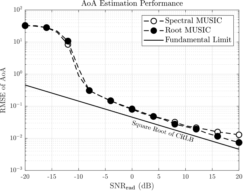
First, we show in Fig. 1 the performance of the first step described in Subsection 3.2.1, whereby AoA is estimated via Spectral and Root MUSIC. The fact that the results show the usual good performance associated with subspace-based methods [14] indicates that the decoupling of AoA and DD estimation does not result in any penalty in terms of accuracy, in spite of the complexity reduction, from $\mathcal{O}\big{(}(N_{a}\cdot N\cdot M)^{3}\big{)}$ for SotA schemes to $\mathcal{O}\big{(}N_{a}^{3}+(NM)^{3}+(N_{a}NM)^{2}\big{)}$ of the proposed method444Derivations are omitted due to page limitations..

Refer to caption
Fig. 1: Performance of decoupled AoA estimation via MUSIC.
Refer to caption
Refer to caption
Fig. 2: Performance of delay and Doppler estimation via LMMSE-improved ML search.

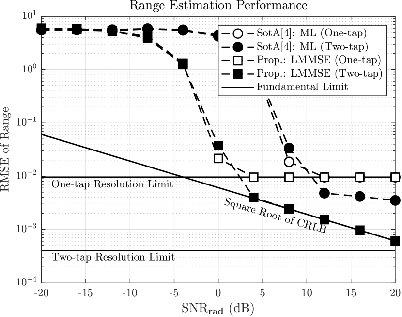
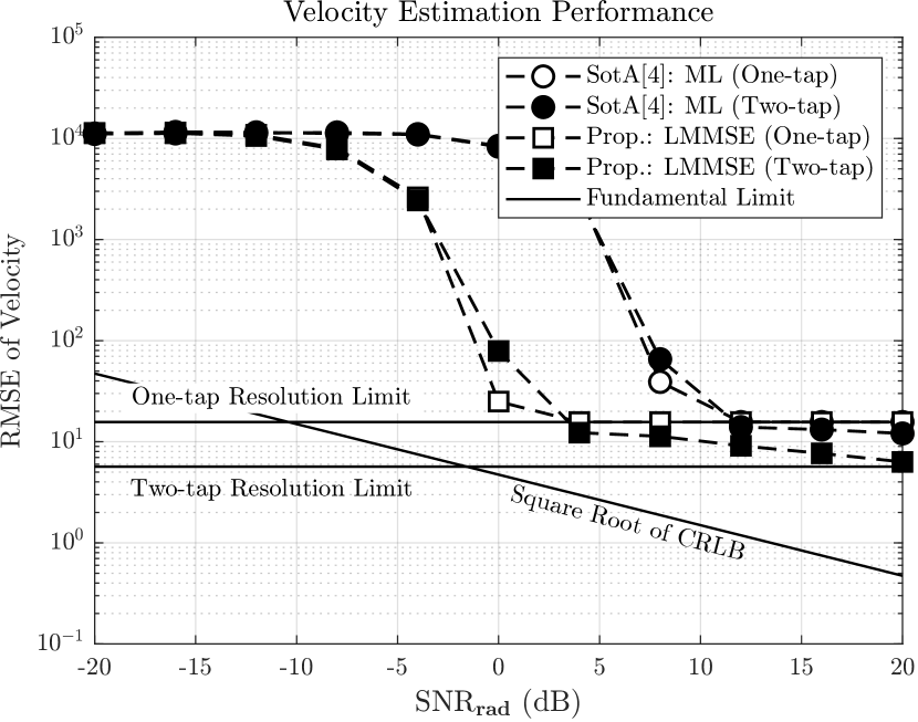
Next, we compare in Fig. 2 the performances of the proposed and SotA [4] methods. It is found that the proposed method significantly improves estimation performance, especially at lower radar SNRs, to the extent that with a one-tap ML search, the RMSE of the proposed method in the range from -5 dB to 0 dB is similar to that of the SotA alternative in the range from 0 dB to 10 dB, indicating a gain of 10 dB in that region. In addition, it is also found that for higher SNRs, the two-tap ML search with the proposed method approaches the CRLB faster than the SotA scheme.

5 Conclusion

We proposed a novel two-step algorithm to estimate the radar parameters from OTFS signals sequentially, with the AoA estimates obtained decoupled from range/velocity. Thanks to the approach, in addition to the resulting lower complexity due to the reduced 2D grid search in the DD domain, the decoupling of AoA and DD estimation enables the incorporation of an LMMSE procedure into the ML estimation of range and velocity, which were shown via simulations to significantly outperform the SotA and approaches the fundamental limits.

References

  • [1] R. Hadani, S. Rakib, M. Tsatsanis, A. Monk, A. J. Goldsmith, A. F. Molisch, and R. Calderbank, “Orthogonal Time Frequency Space Modulation,” in 2017 IEEE Wireless Communications and Networking Conference (WCNC), 2017, pp. 1–6.
  • [2] P. Raviteja, Khoa T. Phan, Yi Hong, and Emanuele Viterbo, “Orthogonal Time Frequency Space (OTFS) Modulation Based Radar System,” in 2019 IEEE Radar Conference (RadarConf), 2019, pp. 1–6.
  • [3] Lorenzo Gaudio, Mari Kobayashi, Giuseppe Caire, and Giulio Colavolpe, “On the Effectiveness of OTFS for Joint Radar Parameter Estimation and Communication,” IEEE Transactions on Wireless Communications, vol. 19, no. 9, pp. 5951–5965, 2020.
  • [4] Lorenzo Gaudio, Mari Kobayashi, Giuseppe Caire, and Giulio Colavolpe, “Joint Radar Target Detection and Parameter Estimation with MIMO OTFS,” in 2020 IEEE Radar Conference (RadarConf20), 2020, pp. 1–6.
  • [5] Akshay S. Bondre and Christ D. Richmond, “Dual-Use of OTFS Architecture for Pulse Doppler Radar Processing,” in 2022 IEEE Radar Conference (RadarConf22), 2022, pp. 1–6.
  • [6] Sai Pradeep Muppaneni, Sandesh Rao Mattu, and A. Chockalingam, “Channel and Radar Parameter Estimation with Fractional Delay-Doppler using OTFS,” IEEE Communications Letters, pp. 1–1, 2023.
  • [7] J. Li and P. Stoica, MIMO Radar Signal Processing, IEEE Press. Wiley, 2009.
  • [8] Duy H. N. Nguyen and Robert W. Heath, “Delay and Doppler processing for multi-target detection with IEEE 802.11 OFDM signaling,” in 2017 IEEE International Conference on Acoustics, Speech and Signal Processing (ICASSP), 2017, pp. 3414–3418.
  • [9] G.A. Vitetta, D.P. Taylor, G. Colavolpe, F. Pancaldi, and P.A. Martin, Wireless Communications: Algorithmic Techniques, Wiley, 2013.
  • [10] Lorenzo Gaudio, Multi-Carrier Modulations Over Sparse Channels: Communication, Channel Estimation, and Radar Sensing, Ph.D. thesis, Technischen Universitat Berlin und der University of Parma in Parma, Italy, 2022.
  • [11] Stefano Fortunati, Luca Sanguinetti, Fulvio Gini, Maria Sabrina Greco, and Braham Himed, “Massive MIMO Radar for Target Detection,” IEEE Transactions on Signal Processing, vol. 68, pp. 859–871, 2020.
  • [12] Benjamin Friedlander, “On Transmit Beamforming for MIMO Radar,” IEEE Transactions on Aerospace Electronic Systems, vol. 48, pp. 3376–3388, 10 2012.
  • [13] Y. Hong, T. Thaj, and E. Viterbo, Delay-Doppler Communications: Principles and Applications, Elsevier Science, 2022.
  • [14] Z. Chen, G. Gokeda, and Y. Yu, Introduction to Direction-of-arrival Estimation, Artech House signal processing library. Artech House, 2010.
  • [15] Veyis Solak, Sultan Aldirmaz-Colak, and Ahmet Serbes, “Fast and Efficient 2-D and K-D DFT-Based Sinusoidal Frequency Estimation,” IEEE Transactions on Signal Processing, vol. 70, pp. 5087–5101, 2022.
  • [16] Chan-Bin Ko and Joon-Ho Lee, “Performance of ESPRIT and Root-MUSIC for Angle-of-Arrival(AoA) Estimation,” in 2018 IEEE World Symposium on Communication Engineering (WSCE), 2018, pp. 49–53.