Brain-inspired Distributed Memorization Learning for Efficient Feature-free Unsupervised Domain Adaptation

Abstract

Compared with gradient based artificial neural networks, biological neural networks usually show a more powerful generalization ability to quickly adapt to unknown environments without using any gradient back-propagation procedure. Inspired by the distributed memory mechanism of human brains, we propose a novel gradient-free Distributed Memorization Learning mechanism, namely DML, to support quick domain adaptation of transferred models. In particular, DML adopts randomly connected neurons to memorize the association of input signals, which are propagated as impulses, and makes the final decision by associating the distributed memories based on their confidence. More importantly, DML is able to perform reinforced memorization based on unlabeled data to quickly adapt to a new domain without heavy fine-tuning of deep features, which makes it very suitable for deploying on edge devices. Experiments based on four cross-domain real-world datasets show that DML can achieve superior performance of real-time domain adaptation compared with traditional gradient based MLP with more than $10\%$ improvement of accuracy while reducing $87\%$ of the timing cost of optimization.

1 Introduction

Nowadays, deep artificial neural networks (ANN) have made many encouraging achievements in pattern recognition and have shown a powerful ability to extract high-dimensional features for effective non-linear classification. The key of ANN is to construct the layers of neurons to fit the complex non-linear function for mapping the input to the output of learning tasks, where the parameters are optimized by using gradient back-propagation to minimize the loss functions.

Most deep ANNs depend on a large scale of labeled data to achieve superior performance, and they are easy to overfit the training set by optimizing a deep network structure with a large number of parameters. Especially in the visual classification tasks, directly transferring a deep model across different domains usually yields a significant drop in performance (Donahue et al., 2014). Recently, some Unsupervised Domain Adaption (UDA) methods have been proposed to utilize the unlabeled data in the target domain to continuously optimize the model. In particular, the pseudo-label based methods (Liang et al., 2020, 2021; Litrico et al., 2023) assign the data in the target domain with pseudo labels to optimize the model in a supervised mode. The clustering based methods (Liang et al., 2020; Li et al., 2021) utilize the relationship between the unlabeled samples to fine-tune the deep model. Meanwhile, as a popular technique, the adversarial learning methods (Ganin & Lempitsky, 2015; Zhang et al., 2018; Yang et al., 2022) are usually used to reduce the diversity of feature distributions between the source domain and target domain.

All of the above methods rely on the back-propagation of the gradient to optimize the deep feature extractor with high timing cost, which are all run on the server side and hard to work on lightweight edge devices. Is it possible to efficiently optimize the model based on the unlabeled data in the target domain by only fine-tuning the mapping between the features and output without time-consuming feature optimization? This is an interesting and practical problem, which is defined as the Feature-free Unsupervised Domain Adaptation (FUDA) problem in this paper.

Compared with ANN, the biological neural networks (BNN) in human brains work much better in this aspect, which can adapt to the new domain quickly and update the network efficiently with no need for large amounts of labeled data. Meanwhile, as pointed out by Hinton (Hinton, 2022), there is no direct proof of explicit gradient back-propagation procedure in BNN. Different from the gradient based function fitting in ANN, BNN seems to take a totally different manner to associate the input and output. The research (Pi et al., 2008) pointed out that memory in brains plays an important role in pattern recognition, which contains three typical stages in the learning and memory process: encoding, storage, and retrieval (Melton, 1963). Some recent research (Roy et al., 2022) showed that the neural cells in brains involved in memory are distributed throughout the entire brain, achieving distributed memory through complex interconnection, rather than being limited to the traditional hippocampus or cerebral cortex.

Inspired by the distributed memory of brains, we try another way to propose a novel gradient-free Distributed Memorization Learning model, namely DML, to support quick domain adaptation, which mimics the behavior of brains in the following aspects. 1) Neurons are connected randomly and signals are transmitted in the form of impulses without continuous activation inspired by the spiking activities in brains (Maass, 1997). 2) Without using the gradient back-propagation, only forwarding is required to process the impulse signal, which is accumulated in the memory units on each neuron and recorded in fuzzy Gaussian distributions to form the memory storage. 3) The distributed memories are retrieved and integrated based on the confidence to make the final decision of classification; 4) Reinforced memorization of the unlabeled data is supported to adapt the model to the target domain efficiently.

Comprehensive experiments based on four cross-domain real-world datasets show that DML can efficiently improve the association between input features and labels in the unlabeled target domain. In particular, compared with the popularly used gradient based neural network MLP, DML can achieve more than $10\%$ improvement of accuracy while reducing $87\%$ of timing cost of optimization in the large-scale dataset VisDA-C (Peng et al., 2017).

The main contributions of this paper are summarized as follows:

• We propose a novel gradient-free Distributed Memorization Learning mechanism, namely DML, for efficient domain adaptation without feature optimization, which models the classification tasks as the distributed memory storage and retrieval procedure on randomly connected neurons.

• We propose an impulse based information transmission mechanism by introducing the accumulation behavior in neurons, so as to achieve the non-linear transformation of signals.

• We utilize multiple Gaussian distributions to simplify the memory storage and adopt the fuzzy memory based on Gaussian blur to reduce the over-fitting problem.

• We propose a reinforced memorization mechanism of DML, which supports lightweight optimization of feature mapping based on unlabeled data in the target domain. The quick optimization without retraining the deep feature extractors makes DML potentially suitable for continuous optimization on edge devices.

2 Related works

2.1 Unsupervised domain adaptation

Unsupervised Domain Adaptation (UDA) methods have been extensively investigated for various application scenarios, including object recognition (Gopalan et al., 2013; Csurka, 2017; Long et al., 2018) and semantic segmentation (Hoffman et al., 2018; Zou et al., 2018; Zhang et al., 2019; Toldo et al., 2020). UDA methods (Pan & Yang, 2009; Candela et al., 2009) focus on training a learner across domains, which is usually achieved by aligning the diverse cross-domain distributions or learning pseudo labels on the target domain.

In particular, Wang et al. (Wang et al., 2023) achieved domain alignment by minimizing the distance between cross-domain samples. Xie et al. (Xie et al., 2022) proposed a collaborative alignment framework to learn domain-invariant representations by utilizing adversarial training or minimizing the Wasserstein distance between two distributions. Hu et al. (Hu & Lee, 2022) introduced a novel distance-of-distance loss that can effectively measure and minimize domain differences without any external supervision. Du et al. (Du et al., 2021) proposed a method of cross-domain gradient difference minimization, which explicitly minimizes the gradient differences generated by the source and target samples.

The adversarial learning is another commonly used technique to minimize the difference in cross-domain features. In particular, Yang et al. (Yang et al., 2022) proposed a dual-module network architecture that incorporates a domain recognition feature module. This architecture undergoes adversarial training by maximizing the loss of feature distribution and minimizing the discrepancy in prediction results. The Collaborative Adversarial Network (CAN) (Zhang et al., 2018) made the feature extractor and classifier cooperate in shallow layers while competing in deep layers to generate specific yet cross-domain features. In order to utilize the discriminative information in classifier labels, the Conditional Adversarial domain adaptation(CDAN) (Long et al., 2018) attempted to align deep features based on classifier labels.

Recently, learning the pseudo labels predicted by the classifiers on the target domain has been proven quite useful for domain adaptation. In particular, SHOT (Liang et al., 2020) adopted self-supervised pseudo-labeling to implicitly align representations from the target domains to the source hypothesis. Litrico M et al.(Litrico et al., 2023) introduced a novel loss re-weighting strategy, assessing the reliability of refined pseudo-labels via estimating their uncertainty. Liang et al. (Liang et al., 2021) proposed a pseudo-labeling framework aimed at reducing classification errors by introducing an auxiliary classifier solely for the target data, thereby enhancing the quality of the pseudo-labels. Li et al.(Li et al., 2021) proposed a cross-domain adaptive clustering method, which introduces an adversarial adaptive clustering loss to facilitate both inter-domain and intra-domain adaptation.

All of the above methods require time-consuming optimization of deep features based on the gradient back-propagation and are only suitable to be run on the server side.

2.2 ANNs without Gradient Back-propagation

Besides the gradient back-propagation based neural networks, there are also some gradient-free network structures, such as the Extreme Learning Machine (ELM) and some of their variants (Cambria et al., 2013; Huang, 2015; Tang et al., 2015). ELM adopted the randomized initialized network for the random projection of features and fit the linear function on these non-linear features. Following a similar idea to ELM, the Broad Learning System (BLS) (Chen & Liu, 2017) extended the network to support incremental learning for newly added dynamic features. The Echo State Network (ESN) (Jaeger, 2002) adopted a random projection network to achieve the non-linear features of time series. The Liquid State Machine (LSM) (Maass et al., 2002) represents a distinct variant of spiking neural networks, characterized by randomly interconnected nodes that concurrently receive inputs from external sources and other nodes within the network. The recently proposed Forward-Forward algorithm (Hinton, 2022) attempted to use two forward processes with positive and negative data respectively to replace the forward and backward processes in the back-propagation algorithms.

Although without using the gradient back-propagation, all of the above methods are still based on the framework of fitting a function to map the input to the output, which is quite different from the distributed memorization of the association between input and output proposed in this paper.

3 METHODOLOGY

3.1 Definition of Feature-free UDA

Most of the visual classification model can be formulated as the function $c(f(x))$, where $f$ is the feature extractor based on the deep models such as ResNet (He et al., 2016) and $c$ is the light-weight classifier such as MLP (Rosenblatt, 1958; Rumelhart et al., 1986) to map the features to output. Given a labeled source domain $D_{s}={(x^{s}_{i},y^{s}_{i})}^{n_{s}}_{i=1}$ and unlabeled target domain $D_{t}={(x^{t}_{i})^{n_{t}}_{i=1}}$, the Feature-free Unsupervised Domain Adaptation (FUDA) aims to transfer the model trained on $D_{s}$ to $D_{t}$, and utilize the unlabeled data in $D_{t}$ to optimize $c$ while freezing the deep feature extractor $f$. FUDA avoids the time-consuming optimization of deep feature extractors and is suitable for the lightweight fine-tuning of visual models on edge devices.

3.2 Overview of Distributed Memorization Learning

As shown in Fig. LABEL:fig:overview, inspired by the memory storage and retrieval stages of human brains, the Distributed Memorization Learning (DML) contains four basic memory-based key procedures: 1) Memory Encoding via impulse based transmission in randomly connected neural network achieves non-linear projection of the input features; 2) Distributed Memory Storage simplified as multiple Gaussian distribution records the association between the features and the labels; 3) Memory Retrieval aims to make prediction by integrating the decision on distributed memory units according to memory confidence; 4) Reinforced Memorization continuously fine-tunes the memories for domain adaptation according to the predicted labels. While freezing the deep feature extractor, DML aims to efficiently optimize the association between the feature input and the labels to address the FUDA problem. The pipeline of DML will be detailed in the following sections.

3.3 Memory Encoding via Random Projection

Inspired by the analysis of the brain network structure (Bassett & Sporns, 2017), which contains highly connected hub nodes as well as sparse linked ones, we adopt a hybrid network topology in DML including three types of nodes: entrance nodes, hub nodes, and bridging nodes. As shown in Fig. LABEL:fig:overview, the entrance nodes accept the input features and are densely connected to the hub nodes. The bridging nodes are randomly and sparsely connected by all of the other nodes. The edges are all directed and the weights on all edges are randomly initialized in the range $[-1,1]$.

After the features are fed to the entranced nodes, the signals are propagated in the network through the edges in multiple rounds. Each node accumulates the incoming signals and is activated intermittently to form the impulse-like output to mimic the spiking activity in brains:

$$h_{i,t+1}=h_{i,t}+\sum_{j\in\mathbb{N}_{i}}O_{j,t}W_{ji}$$ (1)

$$o_{i,t+1}=\left\{\begin{array}[]{ll}h_{i,t+1}&if(h_{i,t+1}>0)\\ 0&else\end{array}\right.$$ (2)

$$h_{i,t+1}=\left\{\begin{array}[]{ll}0&if(h_{i,t+1}>0)\\ h_{i,t+1}&else\end{array}\right.$$ (3)

$$m_{i,t+1}=m_{i,t}+o_{i,t+1}$$ (4)

$$\hat{m}_{i}=m_{i,T}$$ (5)

Here $h_{i,t}$ and $o_{i,t}(0\leq i<N)$ indicate the hidden state and output value individually of the $i^{th}$ node in DML. In the $t^{th}(0\leq t\leq T)$ round of propagation, the signals collected from the predecessor neighbors are accumulated in the hidden state on each node as shown in Eq (1), where the node $j$ is the predecessor neighbor of the node $i$, and $W_{ji}$ is the weight of the edge from $j$ to $i$. While the hidden state of a node is larger than the threshold $0$, the neuron is activated with the value of the hidden state as Eq (2). Otherwise, the output is $0$ in this round. Once the neuron is activated, the hidden state is cleared as Eq (3). The output signal is accumulated as the memory signal $m_{i,t}$ as Eq (4), which will be recorded in the memory storage in the future. When an input feature vector $X=(x_{1},x_{2},...,x_{n})$ is fed to the entrance nodes, the output signal $o_{i,0}(1\leq i\leq n)$ of the entrance nodes are initialized as $x_{i}$, while $o_{i,0}$ of other nodes are all initialized as zero. Meanwhile, $m_{i,0}$ and $h_{i,0}$ are all set as zero at the beginning. The steady memory signal of the node $i$ is defined as $\hat{m}_{i}$ in Eq (5), where $T$ is the max number of the rounds.

Based on the thresholding accumulation of transmitted signals, neurons can generate impulse signals like Fig. 4, which shares the similar intermittent property with the spiking activities in brains (Maass, 1997). On each round of propagation, only a portion of nodes are activated in the network and the left accumulate the signals in their hidden states.

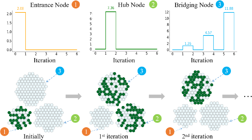
Figure 4: The change of the activation states and the output signals $o_{i,t}$ of the neurons in different iterations of signal propagation. For simplicity, we only show the nodes here while ignoring the connections. The green nodes indicate the activated ones with non-zero output.

3.4 Distributed Memory Storage

Inspired by the distributed memory in brains, each node of DML maintains the memory about the association tween the accepted memory signal $\hat{m}$ and the label $y$ for each input instance as shown in Fig. LABEL:fig:overview-c. The memory unit of the $i^{th}$ neuron node can be modeled as a two-dimensional image $M_{i}$ as shown in Fig. 7, the first dimension of which is the class label $y$ and the other one is the memory signal $\hat{m}$. For each incoming feature vector, which is propagated in the network to achieve the memory signal on each neuron by Eq (5), the association of the memory signal and the label of the instance can be stored by increasing the value of the corresponding pixel in $M_{i}$. However, this trivial implementation of memory storage may lead to a large consumption of computer memory.

To reduce the memory cost, we adopt multiple Gaussian distributions to approximate the memory storage. In particular, for the visual classification tasks, we assume that the distribution of memory signals in the $k^{th}$ class on the $i^{th}$ neuron obeys the Gaussian distribution:

$$Pr(\hat{m}_{i}|y=k)=\frac{1}{\sqrt{2\pi\sigma_{i}^{k}}}exp(-\frac{(\hat{m}_{i}-\mu_{i}^{k})^{2}}{2\sigma_{i}^{k}})$$ (6)

In this way, the storage of memory unit $M_{i}$ can be represented as $C$ Gaussian distribution $\{N(\mu_{i}^{k},\sigma_{i}^{k})|1\leq k\leq C\}$ with $2*C$ learnable parameters, where C is the number of classes.

While training DML on the labeled source domain, the parameters are incrementally updated in batch as follows:

$$\mu_{i}^{k}=\beta\mu^{k}_{i}+(1-\beta)\frac{1}{B}\sum_{b=1}^{B}\hat{m}_{i,b}^{k}$$ (7)

$$\sigma_{i,b}^{k}=\beta\sigma_{i,b}^{k}+(1-\beta)\frac{1}{B}\sum_{b=1}^{B}\sqrt{(\hat{m}_{i,b}^{k}-\mu_{i}^{k})^{2}}$$ (8)

$\beta$ denotes the temperature parameter between batches and $B$ denotes the batch size. $\hat{m}_{i,b}^{k}$ denotes the memory signal received on the $i^{th}$ node while processing the $b^{th}$ instance belong to the $k^{th}$ class.

Meanwhile, the above memory based learning relies on fitting the probability distribution, so a smaller size of the training set or imbalanced label distribution may cause the over-fitting of the distribution function on insufficient samples. To increase the generalization ability of the model, we introduce the Gaussian blur on the memorized Gaussian distribution (Eq (6)) with the Gaussian kernel function $g(x_{1},x_{2})=exp(-\frac{(x_{1}-x_{2})^{2}}{2\sigma_{1}})$ to achieve the fuzzy memory:

$$\begin{split}Q(\hat{m}_{i}|y=k)&=\int_{-\infty}^{+\infty}Pr(\hat{m}|y=k)g(\hat{m},\hat{m}_{i})d\hat{m}\\ &=\frac{\sqrt{\sigma_{1}}}{2\sqrt{2\sigma_{i}^{k}+\sigma_{1}}}exp(-\frac{(\hat{m}_{i}-\mu_{i}^{k})^{2}}{2\sigma_{i}^{k}+\sigma_{1}})\end{split}$$ (9)

3.5 Confidence based Memory Retrieval

The pipeline of memory retrieval on DML is shown in Fig. LABEL:fig:overview-d. After the input features of an instance are fed to the entrance nodes and propagated in the network, the $i^{th}$ node will receive the memory signal $\hat{m}_{i}$ as Eq (5) and retrieve its memory unit to gain the conditional probability inference as follows:

$$Pr(y=k|\hat{m}_{i})=\frac{Q(\hat{m}_{i}|y=k)}{\sum_{c=1}^{C}Q(\hat{m}_{i}|y=c)}$$ (10)

Here $Q(\hat{m}_{i}|y=k)$ indicates the fuzzy memory distribution (Eq (9)) achieved at the memory storage stage. The most likely class label predicted by the $i^{th}$ node is

$$K_{i}=\arg\max\limits_{k}Pr(y=k|\hat{m}_{i})$$ (11)

The confidence of the node to make the prediction can be defined as the likelihood of the memory signal as follows:

$$c_{i}=Q(\hat{m}_{i}|y=K_{i})$$ (12)

The final decision of the whole network is defined as the confidence based fusion of the predictions of all neurons:

$$Pr(y=k|X)=\frac{c_{i}Pr(y=k|\hat{m}_{i})}{\sum_{j}^{N}c_{j}}$$ (13)

3.6 Reinforced Memorization for Domain Adaptation

Following the setting of FUDA, the DML model performs the memory storage on the labeled data from the source domain and is transferred to the unlabeled target domain. Like other pseudo label based algorithms (Qin et al., 2019; Wang & Breckon, 2020; Lai et al., 2023), DML makes prediction on the target domain based on memory retrieval as shown in Fig. LABEL:fig:overview-d to generate the pseudo label of each unlabeled sample $X$:

$$\hat{y}=\arg\max\limits_{k}Pr(y=k|X)$$ (14)

By collecting the pairs of samples and pseudo labels $\{(X,\hat{y})\}$, the memory storage procedure can be conducted as Section 3.4 by continuously updating the parameters as Eq (7) and (8).

As reported by (Litrico et al., 2023), the noise of pseudo labels affects the performance of UDA significantly, which may brings the accumulation of errors and makes the model over-fit the wrong prediction. To reduce the oscillation of the model caused by the noise, we introduce the confidence $E_{i}$ of parameter updating on the node $i$ by measuring the likelihood that the node makes the same prediction as the pseudo label $\hat{y}$:

$$E_{i}(\hat{m}_{i},\hat{y})=Q(\hat{m}_{i}|y=\hat{y})$$ (15)

Then the updating of parameters in Eq (7) and (8) is rewritten as follows:

$$\mu_{i}^{\hat{y}}=\beta\mu^{\hat{y}}+(1-\beta)\frac{1}{B}\sum_{b=1}^{B}E_{i}(\hat{m}_{i,b}^{\hat{y}},\hat{y})\hat{m}_{i,b}^{\hat{y}}$$ (16)

$$\sigma_{i,b}^{\hat{y}}=\beta\sigma_{i,b}^{\hat{y}}+(1-\beta)\frac{1}{B}\sum_{b=1}^{B}E_{i}(\hat{m}_{i,b}^{\hat{y}},\hat{y})\sqrt{(\hat{m}_{i,b}^{\hat{y}}-\mu_{i}^{\hat{y}})^{2}}$$ (17)

The pseudo label with higher confidence on a neuron node will achieve higher weight to update the parameters on the node. After updating the parameters, the model can generate new pseudo labels on the unlabeled data. In this way, the updating can be run in multiple iterations to reinforce the memorization in a self-supervised way, so as to make the learned distribution approach the ground-truth target distribution, which is based on the supervised learning on the target domain, as shown in Fig. 8.

Table 1: Datasets for domain adaptation

Dataset	#Samples	#Domains	#Classes
Office-31	4,110	3	31
Office-Home	15,588	4	65
Digits	178,587	3	10
VisDA-C	207,785	2	12

4 Experiments

4.1 Experimental Setup

Datasets. Comprehensive experiments for FUDA are conducted on four popularly used cross-domain datasets, as shown in Table LABEL:tab:dataset. The details of these datasets are provided in Appendix A. We use the form like $x\rightarrow y$ to indicate the transfer from the source domain $x$ to the target domain $y$ in the following tables.

Table 2: Classification accuracy(%) on the VisDA-C Dataset.

Method	$S\rightarrow R$	$R\rightarrow S$	Avg.
Direct	54.83	65.06	59.95
BLS	59.43	75.05	67.24
KNN	58.60	66.70	62.65
DCT	32.50	47.59	40.05
RFS	49.30	66.22	57.76
MLP	57.84	72.13	64.99
SVM	53.60	68.64	61.12
BAG	59.02	67.43	63.23
NBY	46.75	78.19	62.47
DML(OURS)	62.47	81.68	72.08

Evaluation Metrics. Following the definition of the FUDA challenge, we train the model on the labeled source domain and optimize it based on the unlabeled data in the target domain while freezing the feature extractor. The accuracy of classification and timing cost are evaluated in the target domain.

Baselines. DML is compared with the following baselines, which map the features generated by the feature extractor to the labels:

• The Multi-layer Perceptron (MLP) (Rosenblatt, 1958; Rumelhart et al., 1986) is a variant of the feed-forward artificial neural network optimized by the back-propagation algorithm.

• The Broad Learning System (BLS) (Chen & Liu, 2017) represents a scalable neural network architecture, supporting incremental learning with network expansion.

• The Support Vector Machine (SVM) (Cortes & Vapnik, 1995) aims to identify the optimal hyperplane, so as to maximize the margin between disparate classes of data.

• The K-Nearest Neighbors algorithm (KNN)(Cover & Hart, 1967; Altman, 1992) assigns the labels according to the k-nearest neighboring labeled samples.

• The Decision Tree (DCT) (Quinlan, 1987) adopts a tree-like model, achieved by recursively segmenting the feature space using decision rules.

• The Random Forest (RFS) (Breiman, 2001) integrates multiple decision trees to make the prediction.

• Bagging (BAG) (Breiman, 1996) is an ensemble learning technique that integrates multiple base models trained on different data subsets. Specifically, the KNN is used as the base model for Bagging in the following experiments.

• The Naive Bayesian algorithm (NBY) (Hand & Yu, 2001) is a probabilistic classifier based on the Bayes’ Theorem, under the assumption of mutual independence among features.

Network Configurations. The details of the network configuration and parameter setting in the experiments are provided in the Appendix B.

Table 3: Classification accuracy(%) on the Digits dataset

Method	$S\rightarrow M$	$M\rightarrow U$	$U\rightarrow M$	Avg.
Direct	72.36	79.16	87.27	79.60
BLS	80.80	92.45	93.88	89.04
KNN	77.62	92.07	91.70	87.13
DCT	56.04	77.43	66.24	66.57
RFS	73.83	91.19	88.54	84.52
MLP	77.14	91.57	92.06	86.92
SVM	75.45	92.57	91.64	86.55
BAG	78.36	92.68	92.46	87.83
NBY	81.12	91.75	89.53	87.47
DML(OURS)	82.45	91.18	93.79	89.14

Table 4: Classification accuracy(%) on the Office-31 Dataset

Method	$A\rightarrow D$	$D\rightarrow W$	$W\rightarrow A$	Avg.
Direct	80.52	94.72	63.15	79.04
BLS	80.92	94.84	65.99	80.44
KNN	89.96	94.97	62.80	82.34
DCT	41.37	39.87	24.99	36.18
RFS	81.53	89.69	58.71	77.16
MLP	84.34	94.21	64.71	80.44
SVM	83.53	94.72	62.41	79.62
BAG	87.34	95.60	64.11	82.64
NBY	84.34	92.58	65.32	80.76
DML	92.15	97.48	70.35	86.08

Table 5: Classification accuracy(%) on the Office-Home Dataset

Method	$A\rightarrow C$	$A\rightarrow P$	$A\rightarrow R$	$C\rightarrow A$	$C\rightarrow P$	$C\rightarrow R$	$P\rightarrow A$	$P\rightarrow C$	$P\rightarrow R$	$R\rightarrow A$	$R\rightarrow C$	$R\rightarrow P$	Avg.
Direct	44.60	68.53	75.07	54.10	63.51	65.60	53.15	40.28	72.48	66.17	46.94	78.55	60.75
BLS	47.03	71.59	75.88	55.34	66.19	67.57	54.59	44.33	74.11	65.84	50.20	78.58	62.60
KNN	44.19	67.11	71.63	54.38	64.72	65.64	56.37	45.52	74.59	66.79	52.39	79.21	61.88
DCT	14.39	24.19	30.62	17.26	23.43	26.83	16.89	13.06	31.63	27.28	17.55	39.20	23.53
RFS	40.87	60.04	68.60	48.54	58.75	60.45	47.88	38.95	69.45	63.21	46.85	76.44	56.67
MLP	46.12	66.77	73.24	54.59	64.18	66.26	54.42	43.99	73.79	66.50	50.13	78.85	61.57
SVM	47.15	69.85	74.86	52.32	63.26	64.59	51.59	42.11	72.71	65.18	48.29	77.90	60.82
BAG	45.15	67.65	72.83	52.74	65.58	64.98	56.00	45.29	74.94	66.96	52.00	78.76	61.91
NBY	48.73	72.58	77.55	52.58	67.81	67.82	50.47	40.32	72.05	60.85	47.10	76.66	61.21
DML(OURS)	50.39	76.48	76.91	59.27	71.11	69.65	59.89	47.3	76.47	69.54	53.9	81.03	66.00

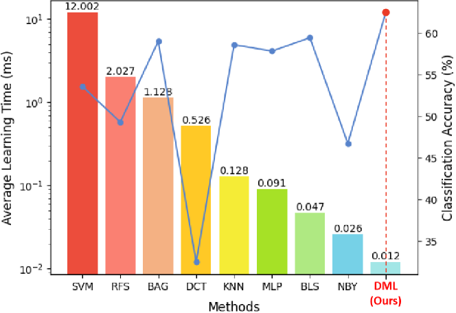
Figure 5: Accuracy versus the average domain adaptation time per instance in different methods on the $S\rightarrow R$ task of the VisDA-C dataset.

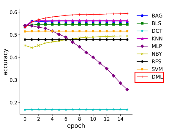
Figure 6: The accuracy in different epochs of domain adaptation on the $P\rightarrow A$ task of the Office-Home dataset.

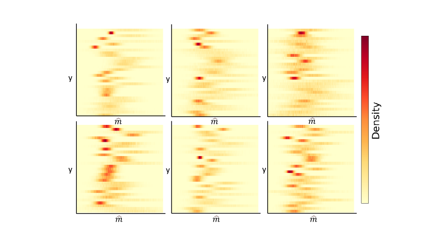
Figure 7: Visualization of the memories on six randomly chosen neurons after training on the Office-31 dataset

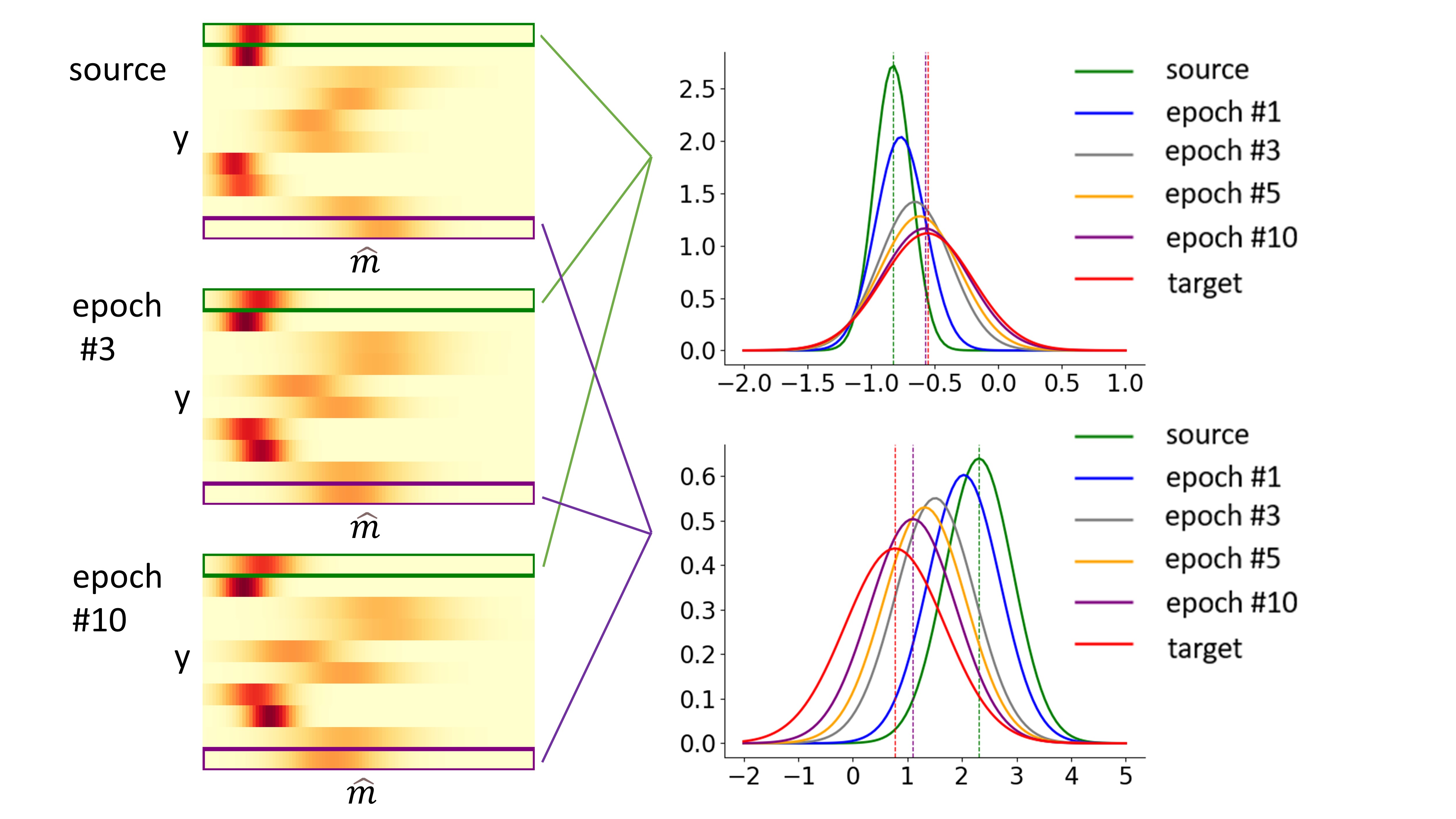
Figure 8: The updating of the memory unit on a neuron while performing the domain adaptation from MNIST to USPS in the Digits dataset.

4.2 Experimental Results

Table 6: Classification accuracy(%) of the variation models, where $G$ indicates the Gaussian blur based fuzzy memory and $C$ indicates the confidence based optimization.

Dataset	base	base+G	base+G+C
Office-31	73.46	85.45	86.08	↑12.62
Office-Home	42.54	64.98	66.00	↑ 23.46
Digits	60.68	88.94	89.14	↑28.46
VisDA-C	35.94	70.97	72.08	↑36.14
average	53.16	77.59	78.33	↑25.17

Tables 2, 3, 4, and 5 show the classification accuracy of each algorithm on the VisDA-C, Digits, Office-31, and Office-Home datasets respectively. It can be observed that DML has the highest average accuracy across all datasets. Particularly on the S $\rightarrow$ R task on the most challenging dataset VisDA-C with the largest size, DML increases the accuracy more than 10% compared with the ANN model MLP. Similarly, in the Office-Home and Office-31 datasets, DML outperforms the other baselines significantly, showcasing its potential as a general classifier in domain adaptation. Fig 5 further illustrates the average time required for self-supervised domain adaptation per sample on the VisDA-C datasets. DML surpasses all other classifiers significantly, reducing 87% time compared with traditional neural network MLP, which is utilized in most UDA methods as the classifier to map deep features to labels in the last layers of the visual models. DML is even twice faster than the light-weight NBY model, indicating its good potential for real-time domain adaptation tasks. More results on all datasets are given in Appendix D.

Fig. 6 further depicts the accuracy of the models over the epochs of learning pseudo labels on the target domain of the Office-Home dataset. More results on all datasets are provided in Appendix E. In all cases, DML can improve the performance steadily, which benefits from the confidence based parameter updating in Eq (16) and (17). It can be also observed that MLP faces a significant drop of performance in some cases, which may be caused by the accumulated errors of noisy pseudo labels.

Visualization Results. Fig. 7 depicts the memory units of randomly chosen neurons intuitively, which show diverse memory patterns on different neurons. Furthermore, Fig. 8 depicts how the memory units evolve along with the iterations of domain adaptation, and highlights the changing of the Gaussian distributions consistent with Eq (7) and (8). After multiple rounds of self-supervised learning on pseudo labels, the distributions effectively approach the target distribution, which corresponds to the model supervised trained using the labels on the target domain. This validates the remarkable effectiveness of DML in FUDA.

Ablation study. The fuzzy memory based on the Gaussian blur in Eq (9) and the confidence based optimization in Eq (16) and (17) play important roles in increasing the robustness of the memory storage and retrieval. Their effectiveness is tested by the ablation studies in Table 6. It can be observed that the Gaussian blur has a great impact on the performance, which confirms the importance of introducing the fuzzy memory to reduce the over-fitting of the distribution function. Table 6 also shows that the combination of all components can achieve the best performance.

Conclusion

In this paper, we propose a novel brain-inspired Distributed Memorization Learning model, namely DML, to support efficient Feature-free Domain Adaptation (FUDA). In particular, DML learns the association between the features and labels based on the distributed memories on the neurons through impulse based information transmission and accumulation. DML is also able to utilize its prediction results on unlabeled data to perform reinforced memorization to support quick domain adaptation. Comprehensive experiments show the superior performance and the low timing cost in DML, which indicates that DML have good potential to be run on edge devices for continuous optimization.

In the future, we will further explore the relationship between the performance and the network topology of DML inspired by biological neural networks. Meanwhile, we will also extend DML to support more learning tasks including the multi-modal FUDA problems to verify the power of distributed memorization.

Appendix A Datasets

• Digits: The classic digit image datasets including 3 different domains: MNIST (LeCun et al., 1998) (M), USPS (Hull, 1994) (U), and SVHN (Netzer et al., 2011) (S). We adopt the evaluation protocol of CyCADA (Hoffman et al., 2018) with three transfer tasks: USPS to MNIST (U $\rightarrow$ M), MNIST to USPS (M $\rightarrow$ U), and SVHN to MNIST (S $\rightarrow$ M).

• Office-31: Office-31 Dataset (Saenko et al., 2010) is the most widely used dataset for visual domain adaptation consisting of 4,110 images from 31 categories collected from three different domains: Amazon (A), Webcam (W) and DSLR (D). All possible combinations of the domains are tested as the transfer tasks: A $\rightarrow$ D, A $\rightarrow$ W, D $\rightarrow$ A, D $\rightarrow$ W, W $\rightarrow$ A, and W $\rightarrow$ D.

• Office-Home: Office-Home dataset (Venkateswara et al., 2017) is a challenging medium-sized benchmark with four distinct domains containing 65 categories: Artistic images (A), Clip Art (C), Product images (P), and Real-World images (R). All possible combinations of the domains are tested as the transfer tasks: A $\rightarrow$ C, A $\rightarrow$ P, A $\rightarrow$ R, C $\rightarrow$ A, C $\rightarrow$ P, C $\rightarrow$ R, P $\rightarrow$ A, P $\rightarrow$ C, P $\rightarrow$ R, R $\rightarrow$ A, R $\rightarrow$ C, and R $\rightarrow$ P.

• VisDA-C: VisDA-C (Peng et al., 2017)is a challenging large-scale benchmark that mainly focuses on the 12-class object recognition task containing two domains: the Synthesis(S) which contains 152 thousand synthetic images generated by rendering 3D models, and the Real(R) which has 55 thousand real object images sampled from Microsoft COCO. All possible combinations of the domains are tested as the transfer tasks: S $\rightarrow$ R, and R $\rightarrow$ S.

Appendix B Network Configuration

Some commonly used deep neural networks are adopted as the feature extractors in the experiments. In particular, we utilize the LeNet-5(LeCun et al., 1998) as the feature extractors for the simple digital recognition task in the Digits dataset. For the object recognition tasks related to the Office-31, Office-Home, and VisDA-C datasets, we adopt the pre-trained ResNet (He et al., 2016) models as feature extractors (ResNet-101 for VisDA-C and ResNet-50 for the other datasets), following the experimental configurations in previous works like (Saito et al., 2017), (Long et al., 2018), (Deng et al., 2019), (Xu et al., 2019), and (Peng et al., 2019).

In the experiments, we adopt mini-batch stochastic gradient descent (SGD) with the momentum as 0.9, weight decay as $1e^{-3}$, and learning rate $\eta=1e^{-2}$. To avoid over-fitting in VisDA-C we set the learning rate to $1e^{-3}$. We further adopt the self-adaptive learning rate following the configures in (Ganin & Lempitsky, 2015; Long et al., 2018; Liang et al., 2020). Besides, the batch size is set to 64 in all datasets. The training epoch for Digits, Office-31, Office-Home, and VisDA-C respectively is set to 30, 100, 50, and 10 empirically. In the domain adaptation step, we use mostly default parameters for the tested baselines. For MLP, the number of hidden nodes is 3096 and the learning rate is 0.01. In DML, the number of hub nodes and bridging nodes are both 50, the in-degree of the bridging nodes is 30, and $T=3$ in Eq.5 by default. To gain better performance, we adjust one hyper-parameter while keeping the rest as default. The number of domain adaptation epochs for VisDA-C, Digits, Office-Home, and Office-31 is set to 16.

Appendix C Full Results of Classification Accuracy on Office-31

The full table of the classification accuracy on the Office-31 datasets covering all cases of domain transferring is shown in Table 7.

Table 7: Classification accuracy(%) of all tasks on the Office-31 Dataset

	$A\rightarrow D$	$A\rightarrow W$	$D\rightarrow A$	$D\rightarrow W$	$W\rightarrow A$	$W\rightarrow D$	Avg.
DT	80.52	76.73	60.53	94.72	63.15	98.59	79.04
BLS	80.92	79.37	62.12	94.84	65.99	99.40	80.44
KNN	89.96	84.78	61.91	94.97	62.80	99.60	82.34
DCT	41.37	35.97	21.44	39.87	24.99	53.41	36.18
RFS	81.53	77.23	56.59	89.69	58.71	99.20	77.16
MLP	84.34	79.75	60.63	94.21	64.71	99.00	80.44
SVM	83.53	77.99	59.89	94.72	62.41	99.20	79.62
BAG	87.34	87.04	62.34	95.60	64.11	99.40	82.64
NBY	84.34	81.64	63.26	92.58	65.32	97.39	80.76
DML	92.15	88.92	68.18	97.48	70.35	99.40	86.08

Appendix D Accuracy versus Timing Cost on all Datasets

Appendix E Accuracy in Different Epochs of Domain Adaptation

Appendix F Parameter Analysis of Network Scale

In order to investigate the impact of network scale on the performance of domain adaptation, we conducted a sensitivity analysis of the number of hub nodes and bridging nodes. To better illustrate the influence of network structure on performance, we excluded the Gaussian blur component here. In Figure 11, we simultaneously increased the quantities of both types of nodes starting from zero, and it can be observed that as the network scale increases, the performance gradually improves. This suggests the significance of the network structure we have proposed.

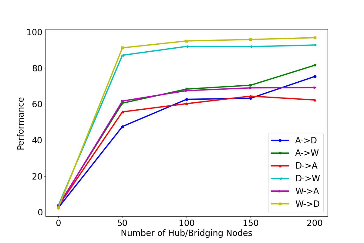
Figure 11: Accuracy versus the number of Hub/Bridging nodes in the Office-31 dataset

References

- Altman (1992) Altman, N. S. An introduction to kernel and nearest-neighbor nonparametric regression. The American Statistician, 46(3):175–185, 1992.
- Bassett & Sporns (2017) Bassett, D. S. and Sporns, O. Network neuroscience. Nature neuroscience, 20(3):353–364, 2017.
- Breiman (1996) Breiman, L. Bagging predictors. Machine learning, 24:123–140, 1996.
- Breiman (2001) Breiman, L. Random forests. Machine learning, 45:5–32, 2001.
- Cambria et al. (2013) Cambria, E., Huang, G.-B., Kasun, L. L. C., Zhou, H., Vong, C. M., Lin, J., Yin, J., Cai, Z., Liu, Q., Li, K., et al. Extreme learning machines [trends & controversies]. IEEE intelligent systems, 28(6):30–59, 2013.
- Candela et al. (2009) Candela, J. Q., Sugiyama, M., Schwaighofer, A., and Lawrence, N. D. Dataset shift in machine learning. The MIT Press, 1:5, 2009.
- Chen & Liu (2017) Chen, C. P. and Liu, Z. Broad learning system: An effective and efficient incremental learning system without the need for deep architecture. IEEE transactions on neural networks and learning systems, 29(1):10–24, 2017.
- Cortes & Vapnik (1995) Cortes, C. and Vapnik, V. Support-vector networks. Machine learning, 20:273–297, 1995.
- Cover & Hart (1967) Cover, T. and Hart, P. Nearest neighbor pattern classification. IEEE transactions on information theory, 13(1):21–27, 1967.
- Csurka (2017) Csurka, G. A comprehensive survey on domain adaptation for visual applications. Domain adaptation in computer vision applications, pp. 1–35, 2017.
- Deng et al. (2019) Deng, Z., Luo, Y., and Zhu, J. Cluster alignment with a teacher for unsupervised domain adaptation. In Proceedings of the IEEE/CVF international conference on computer vision, pp. 9944–9953, 2019.
- Donahue et al. (2014) Donahue, J., Jia, Y., Vinyals, O., Hoffman, J., Zhang, N., Tzeng, E., and Darrell, T. Decaf: A deep convolutional activation feature for generic visual recognition. In International conference on machine learning, pp. 647–655. PMLR, 2014.
- Du et al. (2021) Du, Z., Li, J., Su, H., Zhu, L., and Lu, K. Cross-domain gradient discrepancy minimization for unsupervised domain adaptation. In Proceedings of the IEEE/CVF conference on computer vision and pattern recognition, pp. 3937–3946, 2021.
- Ganin & Lempitsky (2015) Ganin, Y. and Lempitsky, V. Unsupervised domain adaptation by backpropagation. In International conference on machine learning, pp. 1180–1189. PMLR, 2015.
- Gopalan et al. (2013) Gopalan, R., Li, R., and Chellappa, R. Unsupervised adaptation across domain shifts by generating intermediate data representations. IEEE transactions on pattern analysis and machine intelligence, 36(11):2288–2302, 2013.
- Hand & Yu (2001) Hand, D. J. and Yu, K. Idiot’s bayes—not so stupid after all? International statistical review, 69(3):385–398, 2001.
- He et al. (2016) He, K., Zhang, X., Ren, S., and Sun, J. Deep residual learning for image recognition. In Proceedings of the IEEE conference on computer vision and pattern recognition, pp. 770–778, 2016.
- Hinton (2022) Hinton, G. The forward-forward algorithm: Some preliminary investigations. arXiv preprint arXiv:2212.13345, 2022.
- Hoffman et al. (2018) Hoffman, J., Tzeng, E., Park, T., Zhu, J.-Y., Isola, P., Saenko, K., Efros, A., and Darrell, T. Cycada: Cycle-consistent adversarial domain adaptation. In International conference on machine learning, pp. 1989–1998. Pmlr, 2018.
- Hu & Lee (2022) Hu, C. and Lee, G. H. Feature representation learning for unsupervised cross-domain image retrieval. In European Conference on Computer Vision, pp. 529–544. Springer, 2022.
- Huang (2015) Huang, G.-B. What are extreme learning machines? filling the gap between frank rosenblatt’s dream and john von neumann’s puzzle. Cognitive Computation, 7:263–278, 2015.
- Hull (1994) Hull, J. J. A database for handwritten text recognition research. IEEE Transactions on pattern analysis and machine intelligence, 16(5):550–554, 1994.
- Jaeger (2002) Jaeger, H. Adaptive nonlinear system identification with echo state networks. Advances in neural information processing systems, 15, 2002.
- Lai et al. (2023) Lai, Z., Vesdapunt, N., Zhou, N., Wu, J., Huynh, C. P., Li, X., Fu, K. K., and Chuah, C.-N. Padclip: Pseudo-labeling with adaptive debiasing in clip for unsupervised domain adaptation. In Proceedings of the IEEE/CVF International Conference on Computer Vision, pp. 16155–16165, 2023.
- LeCun et al. (1998) LeCun, Y., Bottou, L., Bengio, Y., and Haffner, P. Gradient-based learning applied to document recognition. Proceedings of the IEEE, 86(11):2278–2324, 1998.
- Li et al. (2021) Li, J., Li, G., Shi, Y., and Yu, Y. Cross-domain adaptive clustering for semi-supervised domain adaptation. In Proceedings of the IEEE/CVF Conference on Computer Vision and Pattern Recognition, pp. 2505–2514, 2021.
- Liang et al. (2020) Liang, J., Hu, D., and Feng, J. Do we really need to access the source data? source hypothesis transfer for unsupervised domain adaptation. In International conference on machine learning, pp. 6028–6039. PMLR, 2020.
- Liang et al. (2021) Liang, J., Hu, D., and Feng, J. Domain adaptation with auxiliary target domain-oriented classifier. In Proceedings of the IEEE/CVF conference on computer vision and pattern recognition, pp. 16632–16642, 2021.
- Litrico et al. (2023) Litrico, M., Del Bue, A., and Morerio, P. Guiding pseudo-labels with uncertainty estimation for source-free unsupervised domain adaptation. In Proceedings of the IEEE/CVF Conference on Computer Vision and Pattern Recognition, pp. 7640–7650, 2023.
- Long et al. (2018) Long, M., Cao, Z., Wang, J., and Jordan, M. I. Conditional adversarial domain adaptation. Advances in neural information processing systems, 31, 2018.
- Maass (1997) Maass, W. Networks of spiking neurons: the third generation of neural network models. Neural networks, 10(9):1659–1671, 1997.
- Maass et al. (2002) Maass, W., Natschläger, T., and Markram, H. Real-time computing without stable states: A new framework for neural computation based on perturbations. Neural computation, 14(11):2531–2560, 2002.
- Melton (1963) Melton, A. W. Implications of short-term memory for a general theory of memory. Journal of verbal Learning and verbal Behavior, 2(1):1–21, 1963.
- Netzer et al. (2011) Netzer, Y., Wang, T., Coates, A., Bissacco, A., Wu, B., and Ng, A. Y. Reading digits in natural images with unsupervised feature learning. 2011.
- Pan & Yang (2009) Pan, S. J. and Yang, Q. A survey on transfer learning. IEEE Transactions on knowledge and data engineering, 22(10):1345–1359, 2009.
- Peng et al. (2017) Peng, X., Usman, B., Kaushik, N., Hoffman, J., Wang, D., and Saenko, K. Visda: The visual domain adaptation challenge. arXiv preprint arXiv:1710.06924, 2017.
- Peng et al. (2019) Peng, X., Bai, Q., Xia, X., Huang, Z., Saenko, K., and Wang, B. Moment matching for multi-source domain adaptation. In Proceedings of the IEEE/CVF international conference on computer vision, pp. 1406–1415, 2019.
- Pi et al. (2008) Pi, Y., Liao, W., Liu, M., and Lu, J. Theory of cognitive pattern recognition. Pattern recognition techniques, technology and applications, pp. 626, 2008.
- Qin et al. (2019) Qin, C., Wang, L., Zhang, Y., and Fu, Y. Generatively inferential co-training for unsupervised domain adaptation. In Proceedings of the IEEE/CVF International Conference on Computer Vision Workshops, pp. 0–0, 2019.
- Quinlan (1987) Quinlan, J. R. Generating production rules from decision trees. In ijcai, volume 87, pp. 304–307. Citeseer, 1987.
- Rosenblatt (1958) Rosenblatt, F. The perceptron: a probabilistic model for information storage and organization in the brain. Psychological review, 65(6):386, 1958.
- Roy et al. (2022) Roy, D. S., Park, Y.-G., Kim, M. E., Zhang, Y., Ogawa, S. K., DiNapoli, N., Gu, X., Cho, J. H., Choi, H., Kamentsky, L., et al. Brain-wide mapping reveals that engrams for a single memory are distributed across multiple brain regions. Nature communications, 13(1):1799, 2022.
- Rumelhart et al. (1986) Rumelhart, D. E., Hinton, G. E., and Williams, R. J. Learning representations by back-propagating errors. nature, 323(6088):533–536, 1986.
- Saenko et al. (2010) Saenko, K., Kulis, B., Fritz, M., and Darrell, T. Adapting visual category models to new domains. In Computer Vision–ECCV 2010: 11th European Conference on Computer Vision, Heraklion, Crete, Greece, September 5-11, 2010, Proceedings, Part IV 11, pp. 213–226. Springer, 2010.
- Saito et al. (2017) Saito, K., Ushiku, Y., Harada, T., and Saenko, K. Adversarial dropout regularization. arXiv preprint arXiv:1711.01575, 2017.
- Tang et al. (2015) Tang, J., Deng, C., and Huang, G.-B. Extreme learning machine for multilayer perceptron. IEEE transactions on neural networks and learning systems, 27(4):809–821, 2015.
- Toldo et al. (2020) Toldo, M., Maracani, A., Michieli, U., and Zanuttigh, P. Unsupervised domain adaptation in semantic segmentation: a review. Technologies, 8(2):35, 2020.
- Venkateswara et al. (2017) Venkateswara, H., Eusebio, J., Chakraborty, S., and Panchanathan, S. Deep hashing network for unsupervised domain adaptation. In Proceedings of the IEEE conference on computer vision and pattern recognition, pp. 5018–5027, 2017.
- Wang & Breckon (2020) Wang, Q. and Breckon, T. Unsupervised domain adaptation via structured prediction based selective pseudo-labeling. In Proceedings of the AAAI conference on artificial intelligence, volume 34, pp. 6243–6250, 2020.
- Wang et al. (2023) Wang, Q., Pang, G., Salehi, M., Buntine, W., and Leckie, C. Cross-domain graph anomaly detection via anomaly-aware contrastive alignment. In Proceedings of the AAAI Conference on Artificial Intelligence, volume 37, pp. 4676–4684, 2023.
- Xie et al. (2022) Xie, B., Li, S., Lv, F., Liu, C. H., Wang, G., and Wu, D. A collaborative alignment framework of transferable knowledge extraction for unsupervised domain adaptation. IEEE Transactions on Knowledge and Data Engineering, 2022.
- Xu et al. (2019) Xu, R., Li, G., Yang, J., and Lin, L. Larger norm more transferable: An adaptive feature norm approach for unsupervised domain adaptation. In Proceedings of the IEEE/CVF international conference on computer vision, pp. 1426–1435, 2019.
- Yang et al. (2022) Yang, Y., Zhang, T., Li, G., Kim, T., and Wang, G. An unsupervised domain adaptation model based on dual-module adversarial training. Neurocomputing, 475:102–111, 2022.
- Zhang et al. (2018) Zhang, W., Ouyang, W., Li, W., and Xu, D. Collaborative and adversarial network for unsupervised domain adaptation. In Proceedings of the IEEE conference on computer vision and pattern recognition, pp. 3801–3809, 2018.
- Zhang et al. (2019) Zhang, Y., David, P., Foroosh, H., and Gong, B. A curriculum domain adaptation approach to the semantic segmentation of urban scenes. IEEE transactions on pattern analysis and machine intelligence, 42(8):1823–1841, 2019.
- Zou et al. (2018) Zou, Y., Yu, Z., Kumar, B., and Wang, J. Unsupervised domain adaptation for semantic segmentation via class-balanced self-training. In Proceedings of the European conference on computer vision (ECCV), pp. 289–305, 2018.