Running Coupling and Beta-Functions for HQCD with Heavy and Light Quarks

Irina Ya. Aref’eva^a, Ali Hajilou^a, Pavel Slepov^a and Marina Usova^a

Abstract

We consider running coupling constant and beta-function in holographic models supported by Einstein-dilaton-Maxwell action for heavy and light quarks. We obtain a significant dependence of the running coupling constant $\alpha$ and $\beta$ -function on chemical potential and temperature. At first-order phase transitions, the functions $\alpha$ and $\beta$ -functions undergo jumps depending on temperature and chemical potential. For heavy quarks these jumps depend more sharply on thermodynamic parameters. The magnitude of the jumps increases with decreasing energy scales for both light and heavy quarks.

1 Introduction

The renormalization group (RG) is the approach that refers to changing the physical system as we considered different scales of energy [1, 2, 3]. In fact, RG approach provides systematic picture to describe the physical system with many physical parameters. The dependence of coupling constants of physical system on the energy scale can be described by $\beta$ function of the theory [4, 5, 6, 2]. The RG flows are the variation of fields versus energy scale of the theory. The RG is widely used in various area of the modern theoretical physics [8, 7].

Holographic duality describes a correspondence between a class of strongly coupled field theories and weakly-coupled gravitational theories [9, 10, 11]. Then, one can investigate the strongly coupled regime of gauge theories via holography. In particular, holographic RG flow sets up an explanation of RG flow in terms of gravitational model coupled to dilaton field [12, 13, 14, 15, 16, 17, 18, 19, 20, 21, 22, 23, 24]. The RG flow in this approach has geometrical description and is dual with gravitational solution with specific asymptotic characteristics in such a way that the holographic coordinate corresponds with the energy scale of gauge theory. Therefore, the Hamiltonian evolution in the holographic direction is correspondence with the evolution of the physical system under changing the RG scale.

The studies of holographic RG flow was extensively performed in [19, 20, 21, 22, 23, 24] in context of the QCD applications. The RG flows for the physical systems including chemical potential and asymmetry properties of quark–gluon plasma (QGP) are investigated in [25, 27, 26]. Special interest present the exact holographic RG flows, that exist for higher-dimensional cases [28] as well as for low ones [29, 30, 31].

QCD phase transitions diagram in (temperature, chemical potential)-plane is a challenging and very important task in high energy physics. This is not only an issue of fundamental interest but has also important implications on the description of the early evolution of the Universe [32] and on the study of the interior of compact stellar objects [33, 34]. One of the goal of the experiments on LHC, RHIC, NICA and FAIR is to study the phase structure of the strong-interaction matter under the extreme conditions. Standard theoretical methods for performing QCD calculations, such as perturbation theory no longer works for the strong coupling regime. The lattice theory has a sign problem for non-zero chemical potential calculations, and at its current level cannot provide the suitable information. Therefore to describe physics of the strongly coupled QGP produced in heavy ion collisions (HIC) at RHIC, LHC and NICA (see for example [35]), and future experiments, we need a non-perturbative approach [10, 11].

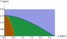
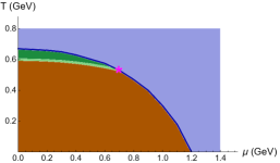
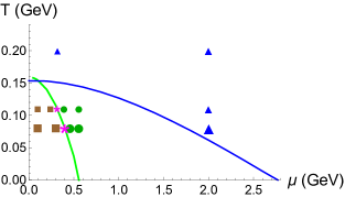
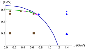
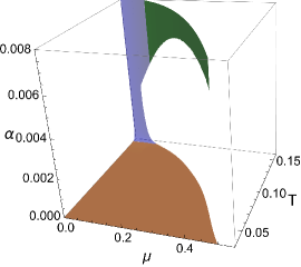
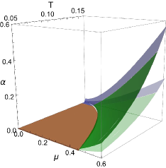
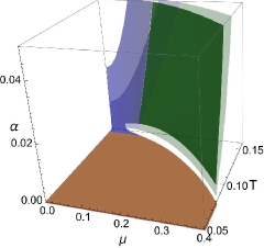
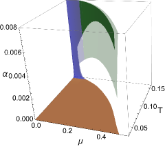
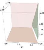
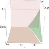
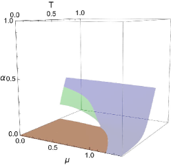
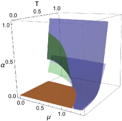
It is expected that QCD phase diagram structure essentially depends on the quark masses, in particular from lattice calculations [36, 37, 38, 39], and some effective phenomenological approach, see for example [40, 41, 35], it is expected that the QCD phase diagrams have the form presented in Fig. 1. Here regions of the hadronic phase are filled by brown color, the regions where quark- gluon phase is realized is filled by blue color. The intermediate regions are filled by the green color. The hardon phase is bounded from above mostly by the first order phase transition for light quark model (light green line in Fig. 1A) and by both the first order phase transition line (light green line in Fig. 1B) and the line dividing confinement and deconfinement phases (blue line in Fig. 1) for heavy quarks. From these plots we see essential difference for light and heavy quarks.

The holographic QCD models for heavy and light quarks constructed in [43, 25, 42, 46, 44, 45] reproduce these phase diagram features at small chemical potential and predict new phenomena for finite chemical potential, in particular, the locations of the critical end points. The goal of this paper to study behaviour of running coupling $\alpha$ and $\beta$ -functions at different phases: quark confinement phases and QGP phase as well as near critical lines.

Refer to caption — Figure 1: Phase structure for light (A) and heavy quarks model (B). Hadronic, QGP and quarkyonic phases are denoted by brown, blue and green regions, respectively. The magenta star shows the critical end point (CEP).

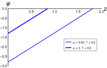
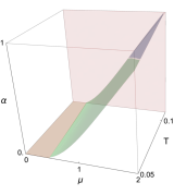
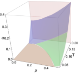
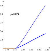
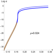
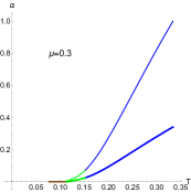
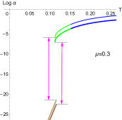
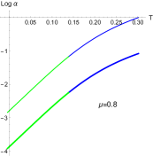
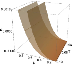
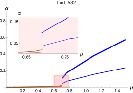
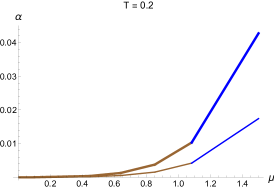
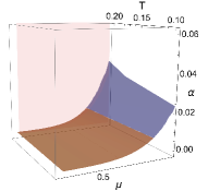
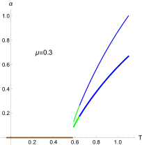
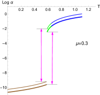
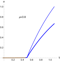
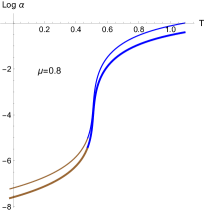
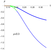
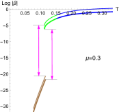
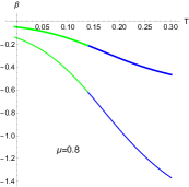
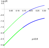
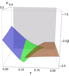
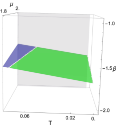
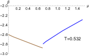
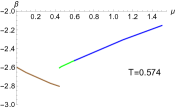
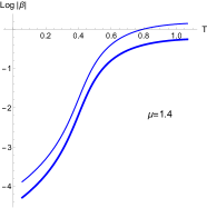
The scattering amplitudes of particles formed during collisions of heavy ions and belonging to the sector of strong interactions significantly depend on the running QCD coupling constants. Typical behavior of the running coupling $\alpha$ at a certain fixed energy scale, different temperatures and chemical potentials is presented in Fig. 2 for light (A) and heavy quarks (B), respectively. Here, in accordance with the color code adopted in Fig. 1, the region of parameters $(\mu,T)$ , where the hadronic phase is realized, is shown in brown, and the region where the quark-gluon phase is realized, shown in blue. Intermediate phases are indicated in green. We see that the running coupling $\alpha(z)$ for light and heavy quarks has jumps on first-order phase transitions. With increasing temperature and chemical potential, the coupling constants for QGP phases increase faster than for hadronic phases. This behaviour of running coupling is in agreement with $\beta$ -function behaviour presented in Fig. 26 and Fig. 33, see Sect.4.1 and Sect.4.2. Here we also see jumps located exactly on the first order phase transition.

This paper is organized as follows:

In Sect. 2 we present 5-dim holographic models for heavy and light quarks and describe thermodynamic properties of these models.

In Sect. 3 we describe running coupling constant for light and heavy quarks models.

In Sect. 4 we describe beta-function for light and heavy quarks models.

In Sect. 5 we describe RG flows constant for light and heavy quarks models.

In Sect. 6 we review our main results.

This work in complemented with:

Appendix A where we describe reconstruction method and solve EOMs,

Appendix B where we present approximation coefficients of potential and gauge kinetic function,

Appendix C with 2D plots of beta-functions on coupling constant.

2 Preliminary

2.1 Holographic model for light quarks

2.1.1 Solution and background

We consider Einstein-Maxwell-scalar (EMS) system with the action [42, 43]

\displaystyle S

\displaystyle=

\displaystyle\frac{1}{16\pi G_{5}}\int d^{5}x\sqrt{-g}\left[R-\frac{\mathfrak{f}_{0}(\varphi)}{4}F^{2}-\frac{1}{2}\partial_{\mu}\varphi\partial^{\mu}\varphi-{\cal V}(\varphi)\right],

(2.1)

where $G_{5}$ is the 5-dimensional Newtonian constant, $F_{\mu\nu}$ is the electromagnetic tensor of the gauge Maxwell field $A_{\mu}$ , $F_{\mu\nu}=\partial_{\mu}A_{\nu}-\partial_{\nu}A_{\mu}$ , $\varphi$ is the scalar (dilaton) field, $\mathfrak{f}_{0}(\varphi)$ is the gauge kinetic function associated to the Maxwell field, ${\cal V}(\varphi)$ is the potential of the scalar field $\varphi$ .

Corresponding to (2.1) equations of motion in general take the following form:

	$\displaystyle\nabla^{2}\varphi$	$\displaystyle=$	$\displaystyle\frac{\partial{\cal V}}{\partial\varphi}+\frac{F^{2}}{4}\frac{\partial\mathfrak{f}_{0}}{\partial\varphi}\leavevmode\nobreak\ ,\quad\nabla_{\mu}\left[\mathfrak{f}_{0}(\varphi)F^{\mu\nu}\right]=0\leavevmode\nobreak\ ,$		(2.2)
	$\displaystyle R_{\mu\nu}-\frac{1}{2}g_{\mu\nu}R$	$\displaystyle=$	$\displaystyle\frac{\mathfrak{f}_{0}(\varphi)}{2}\left(F_{\mu\rho}F^{\rho}_{\nu}-\frac{1}{4}g_{\mu\nu}F^{2}\right)+\frac{1}{2}\left[\partial_{\mu}\varphi\partial_{\nu}\varphi-\frac{1}{2}g_{\mu\nu}(\partial\varphi)^{2}-g_{\mu\nu}{\cal V}(\varphi)\right].$

To solve this system of equations, we consider the ansatz for the metric, scalar field and Maxwell field as [42, 43]

	$\displaystyle ds^{2}=B^{2}(z)\left[-g(z)dt^{2}+d\vec{x}^{2}+\frac{dz^{2}}{g(z)}\right],$		(2.4)
	$\displaystyle B(z)=\frac{e^{A(z)}}{z}\leavevmode\nobreak\ ,\quad\varphi=\varphi(z),\quad A_{\mu}=\left(A_{t}(z)\leavevmode\nobreak\ ,\vec{0},0\right)\leavevmode\nobreak\ ,$		(2.5)

where $\vec{x}=(x_{1},x_{2},x_{3})$ and $A(z)$ is a scale (or warped) factor. Then equations of motion are [42, 43, 25, 50, 44, 49, 46, 47, 48]

	$\displaystyle\varphi^{\prime\prime}+\left(\frac{g^{\prime}}{g}+3A^{\prime}-\frac{3}{z}\right)\varphi^{\prime}+\left(\frac{z^{2}e^{-2A}A^{\prime}_{t}f_{0,\varphi}}{2g}-\frac{e^{2A}V_{\varphi}}{z^{2}g}\right)=0,$		(2.6)
	$\displaystyle A^{\prime\prime}_{t}+\left(\frac{f^{\prime}_{0}}{f_{0}}+A^{\prime}-\frac{1}{z}\right)A^{\prime}_{t}=0,$		(2.7)
	$\displaystyle A^{\prime\prime}-A^{\prime 2}+\frac{2}{z}A^{\prime}+\frac{\varphi^{\prime 2}}{6}=0,$		(2.8)
	$\displaystyle g^{\prime\prime}+\left(3A^{\prime}-\frac{3}{z}\right)g^{\prime}-e^{-2A}z^{2}f_{0}A_{t}^{\prime 2}=0,$		(2.9)
	$\displaystyle A^{\prime\prime}+3A^{\prime 2}+\left(\frac{3g^{\prime}}{2g}-\frac{6}{z}\right)A^{\prime}-\frac{1}{z}\left(\frac{3g^{\prime}}{2g}-\frac{4}{z}\right)+\frac{g^{\prime\prime}}{6g}+\frac{e^{2A}V}{3z^{2}g}=0.$		(2.10)

here all functions depend on the omitted holographic coordinate $z$ and $V(z)={\cal V}(\varphi(z))$ , $V_{\varphi}(z)={\cal V}_{\varphi}(\varphi(z))$ and $f_{0}(z)=\mathfrak{f}_{0}(\varphi(z))$ .

Therefore in isotropic case we have five nontrivial equations: three the Einstein equations, one equation for the scalar field $\varphi$ , one equation for the component of vector potential $A_{t}$ . Eq. (2.6) is the consequences of eq. (2.7) - (2.10) due to the Bianchi identity. Also we have six nonzero functions: two nonzero diagonal components of the metric $g_{MN}$ , one scalar field $\varphi$ , one component of vector potential $A_{t}$ , the potential of scalar field $V$ and one coupling function for the Maxwell tensor $f_{0}(\varphi).$ Therefore we should fix two functions $f_{0}(z)$ and $\mathfrak{b}(z)$ to solve the system of EOM. In this case we obtain four equations (2.7) -(2.10) for four unknown functions ( $\varphi$ , $A_{t}$ , $g(z)$ , $V(z)$ ).

To solve the equations of motion (2.6)-(2.10) the usual boundary conditions (B.C) are used

	$\displaystyle A_{t}(0)=\mu,\quad A_{t}(z_{h})=0,$		(2.11)
	$\displaystyle\quad g(0)=1,\qquad g(z_{h})=0.$		(2.12)

For dilaton field we use

\varphi(z_{h})=0\,.

(2.13)

Note, that if we change B.C. for $\varphi$ the Regge spectrum does not change. Indeed, obtaining linear Regge trajectory one solves Schrodinger equation, i.e (eq. 10 in [51]), that has no dependence on dilaton and just depends on its first and second derivatives.

At zero temperature and zero chemical potential, i.e. $T=\mu=0$ , the vector meson spectrum should satisfy the linear Regge trajectories [51],[42, 43]. Assuming that the Maxwell field $A_{\mu}$ also provides linear Regge trajectories, it is necessary to choose a gauge kinetic function in the form [42]

\displaystyle f_{0}(z)=e^{-c\,z^{2}-A(z)},

(2.14)

where the scale factor $A(z)$ for the light quarks has the form

A(z)=-a\log(bz^{2}+1)\leavevmode\nobreak\ ,

(2.15)

and $a$ , $b$ and $c$ are parameters that can be fitted with experimental data as $a=4.046$ , $b=0.01613$ GeV² and $c=0.227$ GeV² [42].

Under boundary conditions (2.11), (2.12), analytical solutions of the system of equations of motion (2.6)-(2.10) are

$\displaystyle\varphi^{\prime}(z)$	$\displaystyle=$	$\displaystyle\sqrt{-6\Bigg{(}A^{\prime\prime}-A^{\prime 2}+\frac{2}{z}A^{\prime}\Bigg{)}},$	(2.16)
$\displaystyle A_{t}(z)$	$\displaystyle=$	$\displaystyle\mu\frac{e^{cz^{2}}-e^{cz^{2}_{h}}}{1-e^{cz^{2}_{h}}},$	(2.17)
$\displaystyle g(z)$	$\displaystyle=$	$\displaystyle 1-\frac{1}{\int_{0}^{z_{h}}y^{3}e^{-3A}dy}\Bigg{[}\int_{0}^{z}y^{3}e^{-3A}dy-\frac{2c\mu^{2}}{(1-e^{cz_{h}^{2}})^{2}}\Bigg{\|}\begin{matrix}\int_{0}^{z_{h}}y^{3}e^{-3A}dy&\int_{0}^{z_{h}}y^{3}e^{-3A}e^{cy^{2}}dy\\ \int_{z_{h}}^{z}y^{3}e^{-3A}dy&\int_{z_{h}}^{z}y^{3}e^{-3A}e^{cy^{2}}dy\end{matrix}\Bigg{\|}\Bigg{]},$

$\displaystyle V(z)$	$\displaystyle=$	$\displaystyle-3z^{2}ge^{-2A}\Bigg{[}A^{\prime\prime}+3A^{\prime 2}+\Bigg{(}\frac{3g^{\prime}}{2g}-\frac{6}{z}\Bigg{)}A^{\prime}-\frac{1}{z}\Bigg{(}\frac{3g^{\prime}}{2g}-\frac{4}{z}\Bigg{)}+\frac{g^{\prime\prime}}{6g}\Bigg{]}.$	(2.19)

2.1.2 Phase structure for light quarks model

For metric (2.4) temperature can be written as:

\displaystyle\begin{split}T&=\cfrac{|g^{\prime}|}{4\pi}\,\Bigl{|}_{z=z_{h}}\end{split}.

(2.20)

For metric (2.4) and the warp factor (2.5) entropy becomes

\displaystyle s=\frac{\mathfrak{b}^{3/2}(z_{h})}{4z_{h}^{3}}.

(2.21)

The entropy monotonically decreases with horizon growth.

The BH-BH (black hole - black hole, or Hawking-Page-like) phase transition caused by non-monotonicity of the temperature function produces a jump of density $\rho$ , that is a coefficient in $A_{t}$ expansion:

A_{t}=\mu-\rho z^{2}+\dots=\mu-\cfrac{c\mu z^{2}}{1-e^{cz_{h}^{2}}}+\dots,\qquad\rho=-\,\cfrac{c\mu}{1-e^{cz_{h}^{2}}}\,.

(2.22)

To get BH-BH phase transition transition line we need to calculate free energy as a function of temperature:

\displaystyle F=\int_{z_{h}}^{z_{h_{2}}}s\,T^{\prime}dz.

(2.23)

While $T\geq 0$ , i.e for small chemical potentials, we integrate to $z_{h_{2}}=\infty$ . When second horizon where $T=0$ appears, one should integrate to it’s value, i.e. to $z_{h_{2}}=4.609$ . These conditions determine the end-point of the phase diagram, i.e. maximum permissible chemical potential $\mu_{max}$ .

In Fig. 3 the phase diagram of the light quarks model describes two different types of phase transitions. It is very important to note the green line that corresponds to the 1-st order phase transition is obtained using thermodynamics of the theory, i.e. free energy calculations and the blue line corresponds to the confinement/deconfinement phase transition is obtained via Wilson loop calculations [42]. In fact, the phase diagram shows three different phases, i.e. hadronic, quarkyonic and QGP phases are indicated by brown squares, green disks and blue triangles, respectively. All these points are mentioned in an attached table in Fig. 4. We have concentrated on three different fixed temperatures, i.e. $T=0.08,0.11$ and $0.2$ and different values of chemical potential $\mu=0.30,0.31,0.32,0.36,0.394,0.43,0.557$ and $2$ to investigate the running coupling constant and beta-function in different phases of the theory.

In Fig. 4, the dots corresponded to different phases of light quarks phase diagram are depicted in $(z_{h},T)$ -plane. We see that in this figure there are a fewer brown squares, only two of them related to different sizes. This is due to the fact that for very small values of chemical potential the transition temperature occurs at values higher than $T=0.08,0.11$ and $0.2$ . Using this plot, we can obtain the proper $z_{h}$ values associated to definite $\mu$ and $T$ in such a way that we can obtain suitable B.C. for dilaton field as $\varphi\Big{|}_{z=z_{h}(T,\mu)}=0$ for light quarks. Then, we can calculate the running coupling constant and beta-function for light quarks in the next sections.

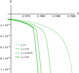
The phase transition for small chemical potential in details is presented in Fig. 5. There is no phase transition for $\mu<0.048$ for light quarks model.

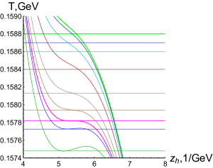
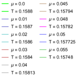
Fig. 4 shows that in isotropic case for $\mu=0$ temperature is a monotonically decreasing function of horizon. Increasing chemical potential one local minimum for temperature as a function of $z_{h}$ appears. As we will see below, this is directly related to the Hawking-page-like phase transition. Indeed, in the isotropic case first-order phase transition for light quarks shouldn’t exist near zero chemical potential and we should see a crossover, Fig. 5. The larger chemical potential is the lesser temperature value at this local minimum becomes. For $\mu\approx 0.557$ local minimum temperature $T_{min}=0$ and second horizon appears.

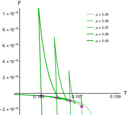
In Fig. 6 Hawking-Page-like phase transition for isotropic case is depicted. In isotropic case BH-BH phase transition starts from a critical point $\mu_{c}=0.04779$ , $T_{c}=0.1578$ .

For the Hawking-Page-like phase transition the free energy should be a multi-valued function of temperature. Graphically it is displayed as a “swallow-tail”. The point where the free energy curve intersects itself determines the Hawking-Page-like phase transition temperature. The larger $\mu$ becomes the more pronounced the “swallow-tail” is (Fig. 6).

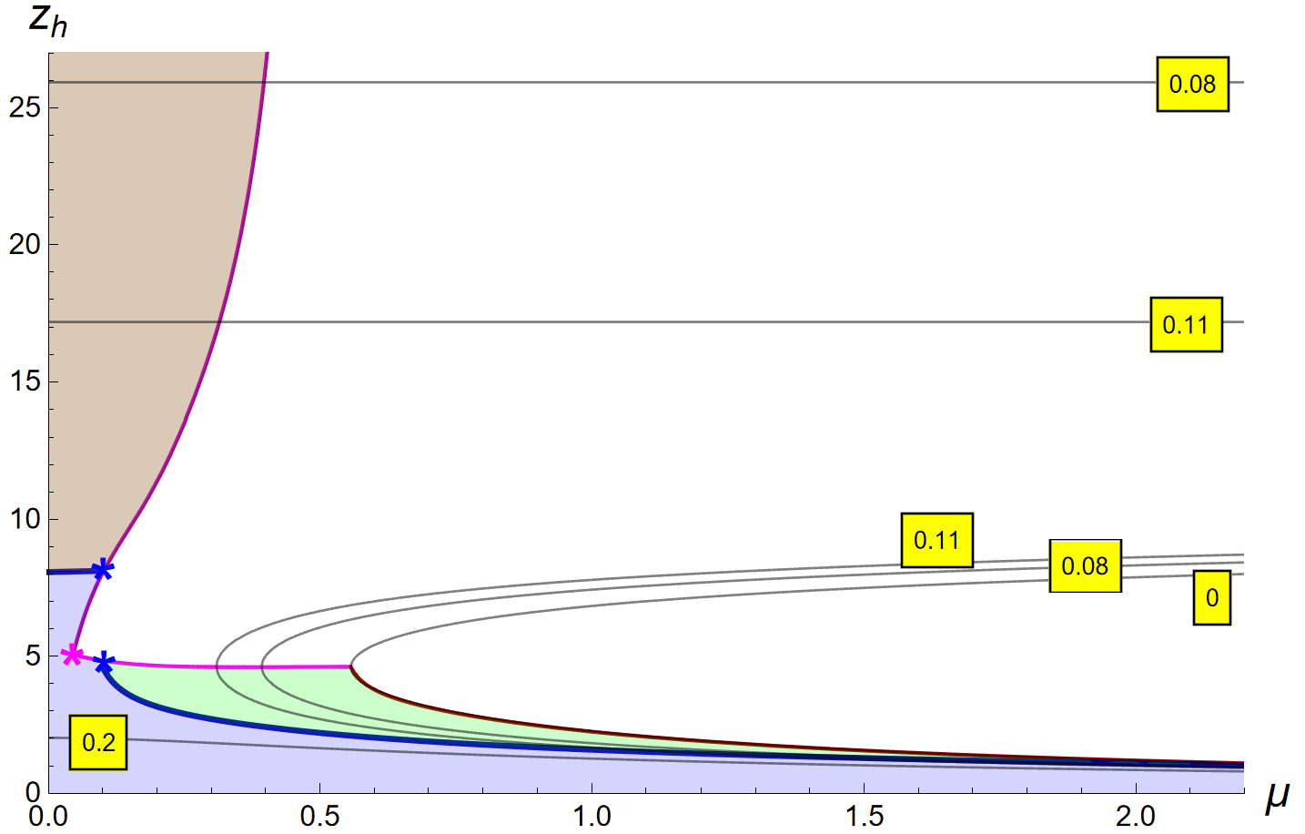
To describe in detail the procedure that is used to construct the 2D $(\mu,z_{h})$ -plane phase transition diagram, Fig. 7, for light quarks model¹¹1This procedure to obtain 2D $(\mu,z_{h})$ -plane is also the same as for heavy quarks model. we consider the following steps:

•

We extract coordinates $(\mu,T)$ of the points corresponding to the 1-st order and confinement/deconfinement phase transition lines from the original phase diagram, i.e. Fig. 3.
•

For each chosen point $(\mu,T)$ on the phase transition lines, we produce $T$ as a function of $z_{h}$ , i.e. $T(z_{h})$ plot, for fixed but different $\mu$ and a line of corresponding constant $T$ .
•
For each point $(\mu,T)$ of original phase diagram Fig. 3, we extract suitable coordinate $z_{h}$ corresponding to the intersection point between constant $T$ and graph of $T(z_{h})$ at fixed $\mu$ in this way:
- –
  
  for the confinement/deconfinement transition - We consider the first intersection at the stable branch of plot $T(z_{h})$ associated with the large black hole. Corresponding result in Fig. 7 are blue lines.
- –
  
  for the 1-st order phase transition - We consider the first intersection at the stable branch of plot $T(z_{h})$ associated with the large black hole and the last intersection at the unstable branch of plot $T(z_{h})$ associated with the small black hole that produce the light magenta line and dark magenta line in Fig. 7, respectively.
- –
  
  for $T=0$ (the 2nd horizon) - We consider different fixed $\mu$ and extract corresponding coordinates $z_{h}$ where the plots $T(z_{h})$ cross $T=0$ line. Corresponding result in Fig. 7 is the red line.
•

Finally, we use the coordinates of the resulted points $(\mu,z_{h})$ to find approximations of functions $z_{h}(\mu)$ for confinement/deconfinement transition line, 1-st order phase transition line and the 2nd horizon to plot Fig. 7. Also, we can produce 3D plot $(\mu,z_{h},T)$ as in Fig. 8.

The phase structure of light quarks model in 2D $(\mu,z_{h})$ -plane in Fig. 7 shows different domains of phases, i.e. QGP, quarkyonic and hadronic correspond to blue, green and brown regions, respectively. The solid blue lines in Fig. 7 correspond to the confinement/deconfinement phase transition line in Fig. 3 obtained via Wilson loop calculations [42]. The solid magenta lines in Fig. 7 correspond to the 1-st order phase transition line in Fig. 3 obtained via free energy calculations [42] and the solid red line corresponds to the second horizon where $T=0$ . All these lines have been obtained via approximation procedure. We see that for $\mu<0.048$ there is crossover region and at $T=0.154$ the phase transition (without any jump) occurs between hadronic and QGP phases. But for $0.0101<\mu<0.560$ when we change the temperature there is a 1-st order phase transition between hadronic and quarkyonic phases with a jump that is clear in Fig. 7. Also, for $\mu>0.101$ by changing the temperature there is the confinement/deconfinement transition between quarkyonic and QGP phases without any jump. Black solid lines show the temperature indicated in yellow squares and the red square corresponds to the intersection of the confinement/deconfinement transition line and 1-st order phase transition which is denoted by the blue stars. The magenta star indicates the end of the 1-st order phase transition.

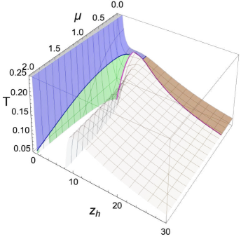
To have a better intuition the 3D phase structure $(\mu,z_{h},T)$ of light quarks in our model is depicted in Fig. 8.

2.2 Holographic model for heavy quarks

2.2.1 Solutions and background

The holographic models describing heavy quarks is described by the same action (2.1) [43, 54], but the warp factor is given by the scalar factor $A(z)$ different from (2.15),

\displaystyle A(z)=-\frac{\mathrm{s}}{3}z^{2}-p\,z^{4}\leavevmode\nobreak\ ,

(2.24)

$\mathrm{s}$ and $p$ are parameters that can be fitted with the experimental data as $\mathrm{s}=1.16$ GeV² and $p=0.273$ GeV⁴. To respect the linear Regge trajectories the gauge kinetic function for heavy quarks model is chosen in the form [43]

\displaystyle\leavevmode\nobreak\ \leavevmode\nobreak\ \leavevmode\nobreak\ \leavevmode\nobreak\ f_{0}(z)=e^{-\mathrm{s}\,z^{2}-A(z)},

(2.25)

compare with (2.14). As in the case of light quarks, the analytic solution for heavy quarks model is obtained by solving the system of equations of motion (2.6)-(2.10) with the boundary conditions (2.11) and (2.12). Therefore, analytical solutions for heavy quarks model are functionally the same, i.e. are given by equations (2.16)-(2.19), only the scale factor $A(z)$ is different as well as constant $c$ is replaced by the constant $\mathrm{s}$ .

2.2.2 Phase structure for heavy quarks model

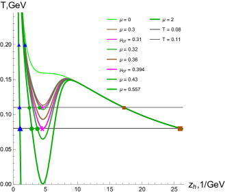
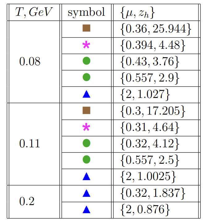
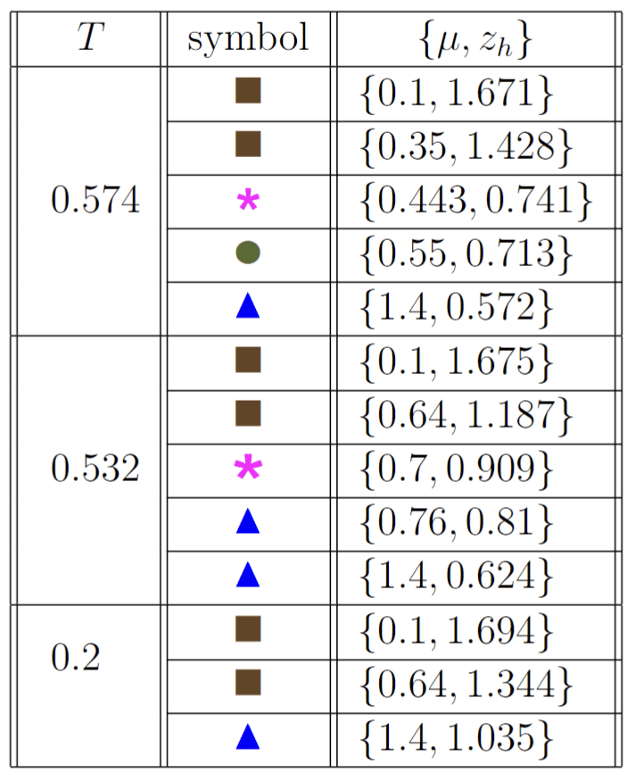
The phase diagram of the heavy quarks model describes two different types of phase transitions Fig. 9. It is very important to note the green line that corresponds to the 1-st order phase transition is obtained using thermodynamics of the theory, i.e. free energy calculations and the blue line corresponds to the confinement/deconfinement phase transition is obtained via Wilson loop calculations [43, 54]. As a matter of fact, the phase diagram shows three different phases, i.e. hadronic, quarkyonic and QGP phases are indicated by brown squares, green disk and blue triangles, respectively. In the phase diagram of the heavy quarks Fig. 9, we concentrated on three different fixed temperatures, i.e. $T=0.2,0.532$ and $0.574$ and different values of chemical potential $\mu=0.10,0.35,0.443,0.55,0.64,0.70,0.76$ and $1.5$ to investigate the running coupling constant and beta-function in different phases of the theory. The points on the 1-st order phase transition line are indicated by magenta stars. All these points are mentioned in a table in Fig. 10C.

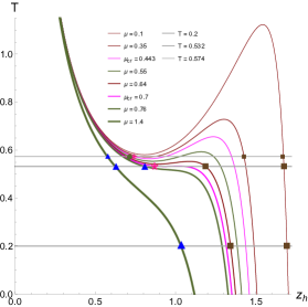
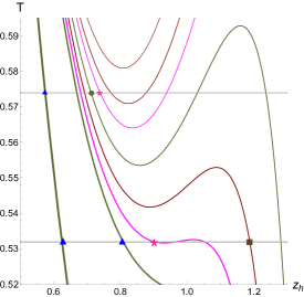
The behavior of the temperature $T$ as a function of $z_{h}$ for heavy quark model for different chemical potentials $\mu$ including different points correspond to different phases is shown in Fig. 10A and its zoom at $0.5\leq z_{h}\leq 1.3$ and $0.52\leq T\leq 0.595$ in Fig. 10B. For $\mu\geq 0.76$ there is no phase transition. Using this plot we can obtain the $z_{h}$ values associated to definite $\mu$ and $T$ in such a way that we can obtain suitable B.C. for dilaton field as $\varphi\Big{|}_{z=z_{h}(T,\mu)}=0$ for heavy quarks. Then we can calculate the running coupling constant and beta-function for heavy quarks in the next sections.

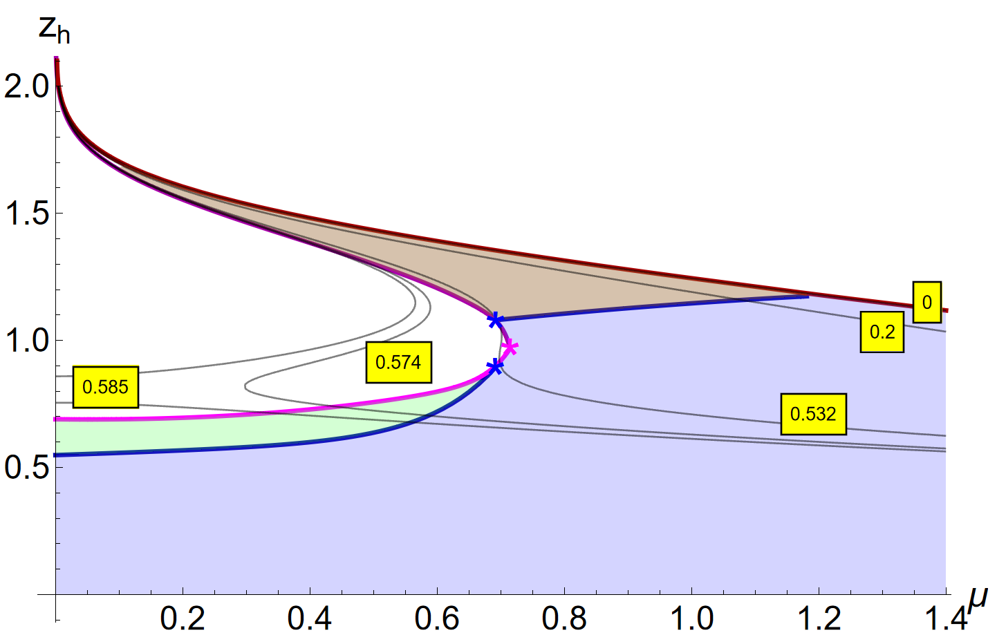
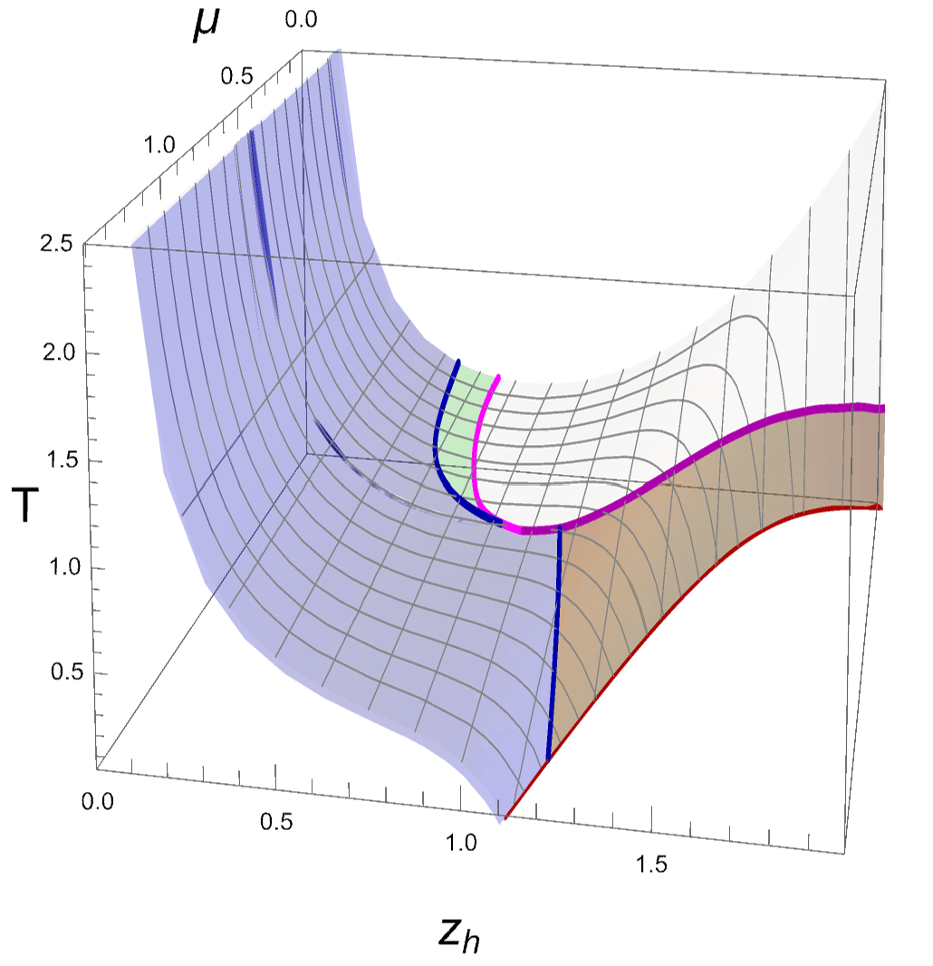
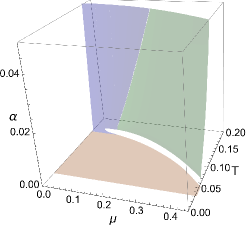
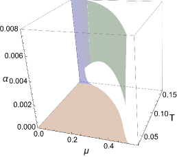
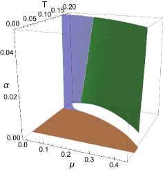
The phase structure of heavy quarks model as 2D $(\mu,z_{h})$ -plane is plotted in Fig. 11 with different domains of phases, i.e. hadronic, quarkyonic and QGP in correspondence with brown, green and blue regions, respectively. The solid thick blue lines in Fig. 11 correspond to the confinement/deconfinement phase transition in Fig. 9 obtained via Wilson loop calculations [43, 54]. The solid thick magenta lines in Fig. 11 correspond to the 1-st order phase transition in Fig. 9 obtained via free energy calculations [43, 54] and the solid thick red line corresponds to the second horizon where $T=0$ . All these lines have been obtained via approximation procedure. For $0<\mu<0.694$ when we change the temperature in Fig. 11 there is a jump between hadronic and quarkyonic phases that represents the 1-st order phase transition, while there is the confinement/deconfinement phase transition between quarkyonic and QGP phases without any jump. Also, for $0.694<\mu<1.181$ there is a confinement/deconfinement phase transition between hadronic and QGP without any jump. The temperature is shown by black solid lines indicated in yellow squares. The intersection of the confinement-deconfinement and 1-st order phase transition lines is denoted by the blue stars. The magenta star indicates CEP that is the end of the 1-st order phase transition. To have a better intuition the 3D phase structure $(\mu,z_{h},T)$ of light quarks model is depicted in Fig. 12.

3 Running coupling constant

The running coupling constant is defined as [19, 20, 53]

\large{\alpha}(z)=e^{\varphi(z)}\,,

(3.1)

where $z$ is the energy scale of the theory and $\varphi$ is the dilaton field that solve the system of equation (2.6)-(2.10). To obtain the running coupling for light and heavy quarks model we have to fix the boundary conditions. We take the following boundary condition for the dilaton field

\varphi\Big{|}_{z=z_{h}(T,\mu)}=0,

(3.2)

where $z_{h}(T,\mu)$ is the value of the horizon for the stable black hole corresponding to given chemical potential $\mu$ and temperature $T$ that can be obtained via $T(z_{h})$ plot described in subsection 2.1.2.

3.1 Running coupling constant for light quarks model

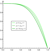
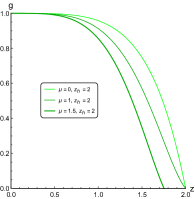
The dilaton field $\varphi(z)$ is depicted in Fig. 13 for $T=0.08,0.11$ and $0.2$ with different values of the chemical potential corresponding to the points of different regions of light quarks phase diagram in Fig 3.

Coupling constant $\alpha(z;\mu,T)$ for light quarks model is depicted in Fig. 14 for two scales of energy $z=1$ , GeV^-1 (A,B) and $z=1.5$ , GeV^-1 (C,D). Hadronic, QGP and quarkyonic phases are denoted by brown, blue and green, respectively. At both scales, coupling constant in hadronic phase is less than in QGP and quarkyonic phases. For very small values of $\mu$ , i.e. crossover region $\alpha$ increases continuously, while for $\mu>0.048$ there is an increment with a jump that shows 1-st order phase transition.

Comparison of coupling constant $\alpha(z)$ for light quarks model in two energy scales $z=1$ GeV^-1 (bright images) and $z=1.5$ GeV^-1 (dark images) are shown in Fig. 15. Hadronic, QGP and quarkyonic phases are denoted by brown, blue and green, respectively. At fixed $\mu$ and $T$ (see panels (A), (B) and (D)) the value of $\alpha$ decreases by increasing energy of system (decreasing $z$ ) and it is compatible with the running coupling of QCD [3]. The jump of $\alpha$ between hadronic and quarkyonic phases is larger for lower energy (larger $z$ ), see panel (C).

Coupling constant $\alpha(z;\mu,T)$ of light quarks at fixed $T=0.08$ (A), $T=0.11$ (B) and $T=0.2$ (C) for different scales of energy $z=0.4$ (thin lines) and $z=1$ (thick lines) are depicted in Fig. 16. Hadronic, QGP and quarkyonic phases are denoted by brown, blue and green lines, respectively. For different fixed $T$ the coupling increases by increasing $\mu$ when our physical system enjoys phase transition from hadronic to quarkyonic and then from quarkyonic to QGP in (A-B). The important result is that there is a jump in panels (A) and (B) when 1-st order phase transition occurs between hadronic and quarkyonic phases anticipated from 3d plots in Fig. 14 and Fig. 19. From (A-B) it is clear that for higher values of energy scale (smaller $z$ ) the jump is bigger in comparison to the lower values of energy scale. For panel (C) there is no phase transition because system is in the QGP phase for all values of $\mu$ .

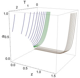
To confirm the results in Fig. 16, the 3D plots for coupling constant $\alpha(z;\mu,T)$ for light quarks in Fig. 17 are depicted at fixed temperature T=0.08 (A,B), T=0.11 (C,D), T=0.2 (E). Fix $T$ is defined by intersection of the plot in Fig. 14 with the planes shown by the red color and for all we set $z=1$ . Hadronic, QGP and quarkyonic phases are denoted by brown, blue and green lines, respectively.

Coupling constant $\alpha(z;\mu,T)$ and $\log\,\alpha(z;\mu,T)$ for light quarks at fixed $\mu=0.024$ (A-B), $\mu=0.3$ (C-D), $\mu=0.8$ (E-F) at different energy scales $z=1$ (thin lines) and $z=0.3$ (thick lines) and different $T$ are shown in Fig. 18. Hadronic, QGP and quarkyonic phases are denoted by brown, blue and green lines, respectively. Magenta arrows in (D) at $\mu=0.3$ show the jumps at the 1-st order phase transition between hadronic and quarkyonic phases, while there is a phase transition without any jump between hadronic and QGP $\mu=0.024$ (A,B), and between quarkyonic and QGP $\mu=0.8$ (E,F). For different fixed $\mu$ the coupling increases when we increase the temperature and physical system experiences different phase transitions from hadronic to quarkyonic and then from quarkyonic to QGP.

A                                                            B

Refer to caption
C                                                            D

E                                                            F

Figure 18: Coupling constant

\alpha(z;\mu,T)

and

\log\,\alpha(z;\mu,T)

for light quarks at fixed

\mu

at different energy scales

z=1

(thin lines) and

z=0.3

(thick lines). Hadronic, QGP and quarkyonic phases are denoted by brown, blue and green lines, respectively. Magenta arrows in D show the jumps at the 1-st order phase transition.

[\mu]=[T]=[z]^{-1}=

GeV.

Coupling constant $\alpha(z;\mu,T)$ for light quarks model at two fixed values of $\mu=0.3$ in Fig. 19A and $\mu=0.8$ in Fig. 19B are plotted. Hadronic, QGP and quarkyonic phases are denoted by brown, blue and green lines, respectively. For all values of changing in energy scale $z$ and fixed $\mu=0.3$ $\alpha$ changes continuously between quarkyonic and QGP, i.e. phase transition occurs with no jump, while there is a jump between hadronic and quarkyonic phases that is 1-st order phase transition. Therefore, coupling constant is sensible to the 1-st order phase transition. At fixed energy scale $z$ by increasing the temperature, $\alpha$ increases from hadronic to quarkyonic and then from quarkyonic to QGP phase. At fixed $\mu=0.8$ there is a continuous phase transition between just two phases, i.e. QGP and quarkyonic.

It is very important to note that to obtain the physical results for coupling constant $\alpha$ for light quarks model as a function of different parameters of the theory in Fig. 14 - 19, we must respect the physical domains of different phases that has already obtained in Fig. 7.

3.2 Running coupling constant for heavy quarks model

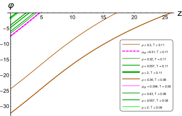
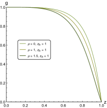
The dilaton field $\varphi(z)$ is depicted in Fig. 20 for $T=0.2,0.532$ and $0.574$ with different values of the chemical potential corresponding to the points of different regions of heavy quarks phase diagram in section 2.2.2.

Coupling constant $\alpha(z;\mu,T)$ for heavy quarks model at two energy scales $z=0.5$ GeV^-1 (dark images) (A), $z=0.3$ GeV^-1 (bright images) (B) and their comparison (C,D) is presented in Fig. 21. Hadronic, QGP and quarkyonic phases are denoted by brown, blue and green, respectively. For $0<\mu<0.7$ there is transition between hadronic and quarkyonic phases as a jump that shows 1-st order phase transition. $\mu=0.7$ denotes the intersection of confinement/deconfinement and 1-st order phase transition lines. For $0.7<\mu<1.18$ the transition occurs continuously between hadronic and QGP phases. At fixed $\mu$ and $T$ (panels (C) and (D)) the value of $\alpha$ increases by decreasing the energy of system (increasing $z$ ) the same as light quarks model and it is compatible with the running coupling of QCD [3]. The jump of $\alpha$ between hadronic and quarkyonic phases is larger for lower energy (larger $z$ ), see panel (C).

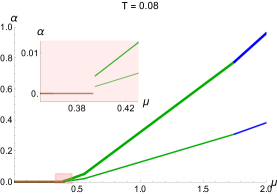
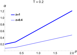
The dependence of coupling constant $\alpha(z;\mu,T)$ on the $\mu$ for heavy quarks at different energy scales $z=0.3$ (thin line) and $z=0.5$ (thick line) and different fixed temperatures $T=0.574$ (A), $T=0.532$ (B), $T=0.2$ (C) is plotted in Fig. 22. Hadronic, QGP and quarkyonic phases are denoted by brown, blue and green, respectively. In (A) the jump is obtained between hadronic and quarkyonic phases and in (B) there is a jump between hadronic and QGP phases.

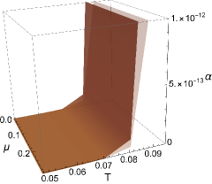
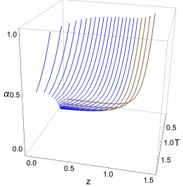
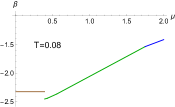
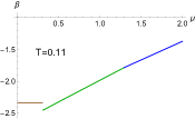
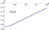
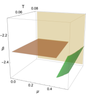
3D representation of Fig. 22, i.e. coupling constant $\alpha(z;\mu,T)$ for heavy quarks at fixed temperature $T=0.574$ (A), $T=0.532$ (B), $T=0.2$ (C) is depicted in Fig. 23. The temperature is defined by intersection of the plot in Fig. 14 with the planes with fixed temperature shown by the light pink color. Hadronic, QGP and quarkyonic phases are denoted by brown, blue and green lines, respectively. We set energy scale as $z=0.5$ . The jumps are shown for (A) between hadronic and quarkyonic for (B) between hadronic and QGP phases.

Coupling constant $\alpha(z;\mu,T)$ and $\log\,\alpha(z;\mu,T)$ for heavy quarks at fixed $\mu=0.3$ and $0.8$ at different energy scales $z=0.3$ (thin lines) and $z=0.2$ (thick lines) is depicted in Fig. 24. Hadronic, QGP and quarkyonic phases are denoted by brown, blue and green lines, respectively. Magenta arrows in (B) with $\mu=0.3$ show the jumps at the 1-st order phase transition between hadronic and quarkyonic phases while at $\mu=0.8$ (C,D) there is a phase transition between hadronic and QGP phases without any jump. The coupling increases when the temperature increases and the physical system undergoes a transition from hadronic to quarkyonic and from quarkyonic to QGP phases.

Coupling constant $\alpha(z;\mu,T)$ for heavy quarks model at $\mu=0.3$ in Fig. 25A and $\mu=0.8$ in Fig. 25B is presented. Hadronic, QGP and quarkyonic phases are denoted by brown, blue and green lines, respectively. At fixed $\mu=0.3$ (in fact $0<\mu<0.7$ ) $\alpha$ changes continuously between quarkyonic and QGP , i.e. phase transition occurs with no jump, while there is a jump between hadronic and quarkyonic phases that is 1-st order phase transition for any range of the energy scale $z$ . It shows that the coupling constant is sensible to the 1-st order phase transition. For each phases in Fig. 25A at fixed $T$ , decreasing the energy (increasing $z$ ) coupling constant increases and vise versa that is compatible with running coupling of QCD [3]. At fixed $\mu=0.8$ there is a continuous phase transition between just two phases, i.e. QGP and hadronic phases.

It is important to note that to obtain the physical results for heavy quarks model for coupling constant $\alpha(z;\mu,T)$ as a function of different parameters of the theory in Fig. 21 - 25, we considered the physical domains of different phases heavy quarks that has been already obtained in Fig. 11. The very important result is that coupling constant as a physical quantity feels the 1-st order phase transition line and undergoes a jump at this line and this jump for heavy quarks are more sharply depends on thermodynamic parameters.

4 Beta-Function

Beta-function, $\beta(\alpha)$ , encodes the dependence of coupling constant $\alpha$ on the energy scale of the physical system. Holographic $\beta$ -function is given by [12, 19, 52]

\beta(\alpha)=3\,\alpha\,X\,,

(4.1)

where $\alpha(z)$ is defined in (3.1) and $X$ is a new dynamical variable defined as [26, 28, 27]

X(z)=\frac{\dot{\varphi}B}{3\dot{B}}\,,

(4.2)

where $B(z)$ is defined in (2.5) and $\varphi$ for light quarks model is obtained in (A.2.1).

4.1 Beta-Function for light quarks model

4.1.1 $\beta$ -function as a function of thermodynamic parameters at fixed energy scale

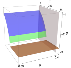
The main result of the light quarks is presented as the dependence of $\beta$ -function on the temperature and the chemical potential at fixed coupling constant $\alpha=1$ in Fig. 26. The choice of fixed coupling constant $\alpha=1$ can be obtained considering energy scale at the horizon i.e. $z=z_{h}$ . Clearly, we see the jumps in the values of the $\beta$ -function at the 1-st order phase transition between hadronic and quarkyonic phases. Therefore, this result shows a very important point that $\beta$ -function as a physical quantity can feel the 1-st order phase transition. Fig. 26 shows that for very small values of $\mu$ in crossover region there is continuous phase transition between hadronic and QGP phases and also a continuous phase transition between quarkyonic and QGP.

The dependence of the light quarks $\beta$ -function on $\mu$ for fixed $T=0.08,0.11$ and $0.2$ at fixed coupling constant $\alpha=1$ is plotted in Fig. 27. Hadronic, QGP and quarkyonic phases are denoted by brown, blue and green colors, respectively. In $T=0.08$ (A) and $T=0.11$ (B) there is a jump between hadronic and quarkyonic phases and physical system experiences the 1-st order phase transition at $\mu=0.4$ and $\mu=0.32$ , respectively. In addition, in (A,B) $\beta$ -function is almost fixed until the jump and then the $\beta$ -function increases monotonically and phase transition occurs between quarkyonic and QGP phases without any jump. In $T=0.2$ (C) just QGP phase dominates and there is no phase transition as well as increasing $\mu$ increases the $\beta$ -function monotonically.

In Fig. 28 the 3D representation of Fig. 27, i.e. $\beta(z;\mu,T)$ for light quarks at fixed temperatures $T=0.08$ (A), $T=0.11$ (B), $T=0.2$ (C) is plotted. The constant $T$ are defined by intersection of the plot in Fig. 26 with the planes at fixed temperature shown by the light orange color. Hadronic, QGP and quarkyonic phases are denoted by brown, blue and green lines, respectively. We fixed coupling constant $\alpha=1$ .

The temperature dependence of $\beta$ -function, $\beta(z;\mu,T)$ and $\log\,\beta(z;\mu,T)$ for light quarks model at fixed $\mu=0.024$ (A,B), $\mu=0.3$ (C,D) $\mu=0.8$ (E,F) and different energy scales $z=1$ (thin lines) and $z=0.3$ (thick lines) is depicted in Fig. 29. Hadronic, QGP and quarkyonic phases are denoted by brown, blue and green lines, respectively. Magenta arrows in D show that $\beta$ -function feels the jumps at the 1-st order phase transition between hadronic and quarkyonic phases. In $\mu=0.024$ (A) and $\mu=0.8$ (E) there is a phase transition without any jump between hadronic to QGP and between quarkyonic to QGP, respectively. $\beta$ -function decreases with increasing $T$ for fixed $\mu$ . In addition, for larger energy scale (smaller $z$ ) in the system, the $\beta$ -function decreases more sharply.

In Fig. 30 the 3D representation for the dependence of the light quarks $\beta$ -function on $T$ are obtained by intersections of 3D plot presented in Fig. 26 with gray planes at fixed $\mu=0.4$ (A) and $\mu=2$ (B). Hadronic, QGP and quarkyonic phases are denoted by brown, blue and green colors, respectively. In (A) the jump occurs at $T_{jump}=0.078,\,\mu=0.4$ . We fixed coupling constant $\alpha=1$ . The $\beta$ -function at a fixed $\mu=0.4$ first remains almost constant in the hadronic phase until a jump at $T_{jump}=0.078$ , then increases with increasing temperature $T$ . In (B) there is a continues phase transition between quarkyonic and QGP phases by increasing the temperature and $\beta$ -function increases as well.

4.1.2 $\beta$ function as function of $\alpha$ at different thermodynamic parameters

To see these jumps in the values of the $\beta$ -function during the 1-st order phase transition on different scales parameterized by the holographic coordinate $z$ , we represent the beta-function $\beta(\alpha;\mu,T)$ for light quarks at fixed $\mu=0.02$ (A), its zoom (B) and $\mu=0.3$ (C), its zoom (D) in Fig. 31. Hadronic, QGP and quarkyonic phases are denoted by brown, blue and green colors, respectively. Red solid lines denote the fixed temperatures. In Fig. 31 A and B, $\beta(\alpha;\mu,T)$ for light quark model is plotted at $\mu=0.02$ in the crossover region where the 1-st order phase transition does not occur, while confinement/deconfinement phase transition occurs with out any jump between hadronic and QGP phases. In Fig. 31. C and D, $\beta(\alpha;\mu,T)$ is plotted at $\mu=0.3$ . For this value of the chemical potential the 1-st order phase transition occurs at $T=0.1145$ .

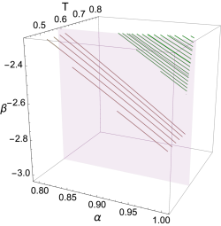
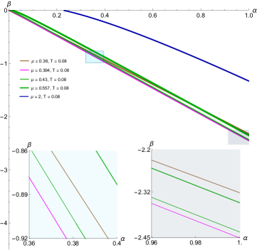
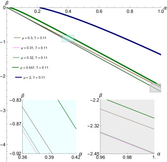
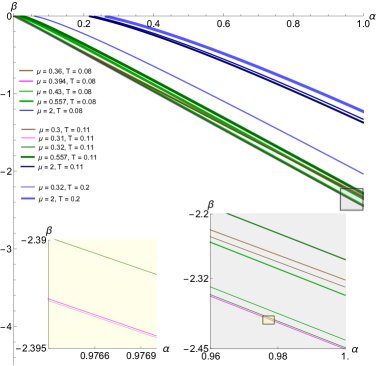
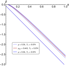
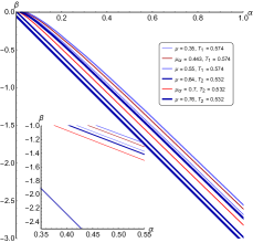
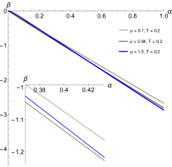
Beta-function $\beta(\alpha;\mu,T)$ for light quarks at fixed $\mu=0.3$ (A) and its zoom at the first order phase transition temperature $T=0.113$ (B) is plotted in Fig. 32. Hadronic, QGP and quarkyonic phases are denoted by brown, blue and green colors, respectively. The plane with $T=0.113$ is shown by light grey. The jump that discussed in Fig. 31 and the phase transition can be seen in detail in Fig. 32. Both figures show the linear dependence of $\beta$ -function on $\alpha$ at different $T$ for hadronic and QGP phases. In Fig. 31-Fig. 32, we see that the dependence of $\beta$ -function on $\alpha$ is mainly linear with a slope depending on the parameters $T$ and $\mu$ . To make this relationship more clear, $\beta$ -function as a function of $\alpha$ for different values of $T$ and $\mu$ on separate graphs is plotted, see Fig. 58 - Fig. 60 in Appendix C.

It is needed to emphasize that to obtain the physical results for $\beta$ -function for light quarks model as a function of different parameters of the theory in Fig. 26 - 32, we must respect the physical domains of different phases for light quarks that has already been obtained in Fig. 7.

4.2 Beta-Function for heavy quarks model

4.2.1 $\beta$ -function as a function of thermodynamic parameters at fixed energy scale

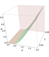
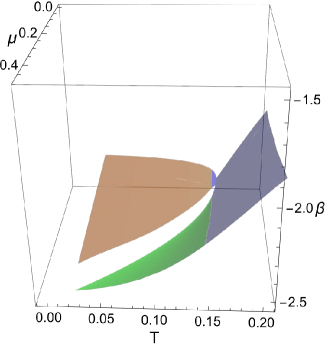
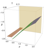
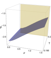
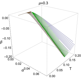
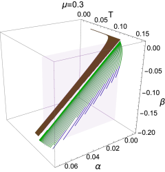
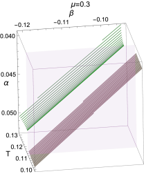
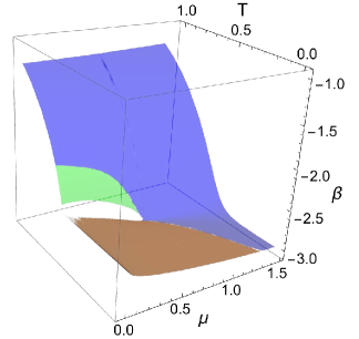
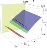
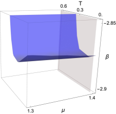
The main result of the heavy quarks model is presented as the dependence of $\beta$ -function on the temperature and the chemical potential at fixed coupling constant $\alpha=1$ in Fig. 33. The choice of fixed coupling constant $\alpha=1$ can be obtained considering energy scale at the horizon i.e. $z=z_{h}$ . Clearly, we see the jumps in the values of the $\beta$ -function at the 1-st order phase transition between hadronic and quarkyonic phases. Therefore, this result shows a very important point that $\beta$ -function as a physical quantity can feel the 1-st order phase transition.

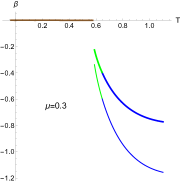
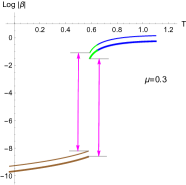
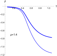
The dependence of the heavy quarks $\beta$ -function on $\mu$ for fixed $T=0.2$ (A), $T=0.532$ (B) and $T=0.574$ (C) at fixed coupling constant $\alpha=1$ is plotted in Fig. 34. Hadronic, QGP and quarkyonic phases are denoted by brown, blue and green colors, respectively. In $T=0.2$ (A) there is a phase transition between hadronic and QGP phases without any jump. In addition, increasing $\mu$ decreases the $\beta$ -function monotonically. In $T=0.532$ (B) there is a jump between hadronic and QGP phases and in $T=0.574$ (C) there is a jump between hadronic and quarkyonic phases. In (B,C) the physical system experiences the 1-st order phase transition at $\mu=0.7$ and $\mu=0.45$ , respectively. In addition, in (B,C) the $\beta$ -function decreases by increasing $\mu$ until the jump and then increases. In (A) the $\beta$ -function decreases by increasing $\mu$ .

In Fig. 35 the 3D representation of Fig. 34, i.e. $\beta(z;\mu,T)$ for heavy quarks at fixed temperatures $T=0.2$ (A), $T=0.532$ (B), $T=0.574$ (C) that are defined by intersection of the plot in Fig. 33 with the planes with fixed temperature shown by the light orange color. Hadronic, QGP and quarkyonic phases are denoted by brown, blue and green lines, respectively. We fixed coupling constant $\alpha=1$ .

The temperature dependence of $\beta$ -function, $\beta(z;\mu,T)$ and $\log\,\beta(z;\mu,T)$ for heavy quarks model at fixed $\mu=0.3$ (A,B), $\mu=1.4$ (C,D) at different energy scales $z=0.3$ (thin lines) and $z=0.2$ (thick lines) is depicted in Fig. 36. Hadronic, QGP and quarkyonic phases are denoted by brown, blue and green lines, respectively. Magenta arrows in (B) show that the jumps at the 1-st order phase transition between hadronic and quarkyonic phases. In $\mu=1.4$ (C) there is no phase transition because the QGP phase is dominated. $\beta$ -function is negative and decreases with increasing $T$ at fixed $\mu$ . In addition, for smaller energy scale (larger $z$ ) in the system, the $\beta$ -function decreases more sharply.

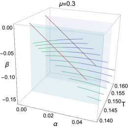
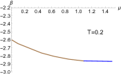
In Fig. 37 3D representation for the dependence of the heavy quarks $\beta$ -function on $T$ are obtained by intersections of 3D plot presented in Fig. 33 with gray planes at fixed $\mu=0.4$ (A) and $\mu=1.4$ (B). We fixed coupling constant $\alpha=1$ . Hadronic, QGP and quarkyonic phases are denoted by brown, blue and green colors, respectively. In (A) the jump occurs at $T_{jump}=0.58,\,\mu=0.4$ between hadronic and quarkyonic phases that shows the 1-st order phase transition. In (A) before jumping the $\beta$ -function almost is constant and after jump increases with increasing the temperature. In (B) the QGP phase is dominated with no phase transition and $\beta$ -function has a local minimum.

4.2.2 $\beta$ -function as a function of $\alpha$ at different thermodynamic parameters

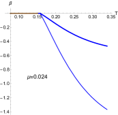
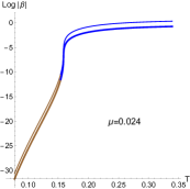
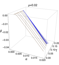
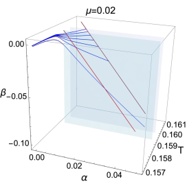
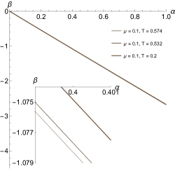
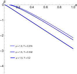
To investigate the jumps in the values of the $\beta$ -function during the 1-st order phase transition on different scales parameterized by the holographic coordinate $z$ , we represent the beta-function $\beta(\alpha;\mu,T)$ for heavy quarks in Fig. 38. Hadronic, QGP and quarkyonic phases are denoted by brown, blue and green colors, respectively. Red solid lines denote the fixed temperatures. In Fig. 38 A there is confinement/deconfinement phase transition occurs without any jump between quarkyonic and QGP phases and there is a jump between hadronic and quarkyonic phases as a 1-st order phase transition. To see the jump in detail Fig. 38B is depicted and the light grey surface shows the $T_{jump}=0.585$ where the 1-st order phase transition occurs.

In Fig. 38, the dependence of $\beta$ -function on $\alpha$ is mostly linear with a slope depending on the parameters $T$ and $\mu$ . To have more clarification, we plotted $\beta$ -function as a function of $\alpha$ for different values of $T$ and $\mu$ on separate graphs, see Fig. 61 and Fig. 62 in Appendix C.

It is very important to note that our results show at the 1-st order phase transition $\beta$ -function experiences the jumps depending on the parameters of theory, i.e $T$ and $\mu$ . In fact, the $\beta$ -function can feel the the 1-st order phase transition. In particular, to obtain the physical results for $\beta$ -function for heavy quarks model as a function of different parameters of the theory in Fig. 33 - 38, we must respect the physical domains of different phases for heavy quarks that has already been obtained in Fig. 11.

5 RG flow

5.1 RG flow equation for zero temperature and zero chemical potential

Let us consider zero temperature and zero chemical potential case. One defines a new dynamical variable [19, 20, 26, 28, 27]

X(z)=\frac{\dot{\varphi}B}{3\dot{B}},

(5.1)

and consider ${\cal X}$ such that

X(z)={\cal X}(\varphi(z)).

(5.2)

The function ${\cal X}(\varphi)$ satisfies the the following equation

\displaystyle\frac{d{\cal X}}{d\varphi}

\displaystyle=

\displaystyle-\frac{4}{3}\left(1-\frac{3}{8}{\cal X}^{2}\right)\left(1+\frac{1}{{\cal X}}\frac{\partial_{\varphi}{\cal V}(\varphi)}{{\cal V}(\varphi)}\right).

(5.3)

that following from EOM (2.6)-(2.10). One calls this equation the RG flow equation [19, 20], since ${\cal X}$ is related with $\beta$ -function defined as

\beta=3\,\alpha\,X,

(5.4)

where $X$ is given by (5.1) and $\alpha$ is the running coupling that is given by equation (3.1).

5.1.1 RG flow for light quarks model

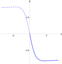
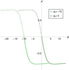
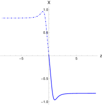
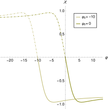
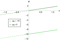
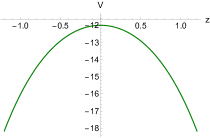
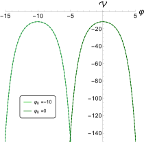
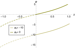
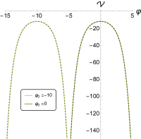
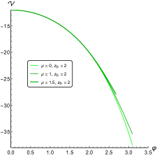
The plots of $X(z)$ given by equation (5.1) and ${\cal X}={\cal X}(\varphi)$ are presented in Fig. 39A and Fig. 39B, respectively. Fig. 39B is recovered from equations (5.1) and (A.2.1).

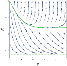
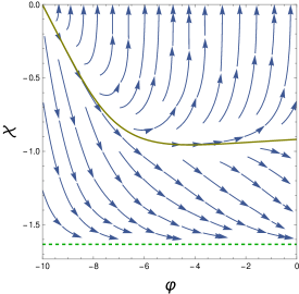
In Fig. 40 RG flows for light quark in isotropic background with $T=0$ and $\mu=0$ corresponding to ${\cal V}(\varphi)$ with different B.C. $\varphi_{0}=-10$ (A) and $\varphi_{0}=0$ (B) are presented. The blue and red lines depict the function ${\cal X}$ presented in

In Fig. 40 RG flows for the case $T=0,$ $\mu=0$ corresponding to ${\cal V}(\varphi)$ with different boundary conditions: $\varphi_{0}=-10$ (A) and $\varphi_{0}=0$ (B) are shown. The blue and green lines depict the function ${\cal X}$ presented in Fig. 39B and recovered from (5.1) and (A.2.1). Parts of these lines with $\varphi>\varphi_{0}$ act as a repulsor and parts with $\varphi<\varphi_{0}$ as an attractor (this is actually the non-physical part). We see that in Fig. 39A $X(z)\to 0$ for $z\to 0$ . In Fig. 39B ${\cal X}(\varphi)\to 0$ for $\varphi\to\varphi_{0}$ . 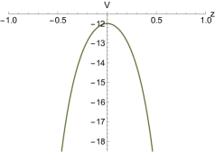This happends because (5.1) $X(z)\sim\dot{\varphi}B/\dot{B}$ , $\dot{\varphi}\to const$ and $B/\dot{B}\to 0$ for $z\to 0$ .

In Fig. 40 we see the comparison between our solution and phase portrait of (5.8). Also ${\cal X}(\varphi)\to 0$ for $\varphi\to\varphi_{0}$ . Here ${\cal X}(\varphi)\to const$ for $\varphi\to 0$ . In Fig. 40 the approximation for the potential is checked only for $-23.5\leq\varphi\leq 3.5$ see Fig. 49. So we can trust the stream plot only for $|\varphi+10|\leq 13$ .

5.1.2 RG flow for heavy quarks model

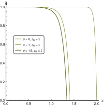
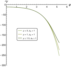
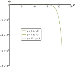
The plots of $X(z)$ given by equation (5.1) and ${\cal X}={\cal X}(\varphi)$ for heavy quarks model are presented in Fig. 41A and Fig. 41B, respectively. RG flows for heavy quarks at $T=0$ and $\mu=0$ is depicted in Fig. 42. In this plot the approximation for the potential is valid only for $-23.5\leq\varphi\leq 3.5$ for $\varphi_{0}=-10$ , see Fig. 51.

5.2 RG flow equations for non-zero temperature and non-zero chemical potential

Introducing new variables

$\displaystyle X$	$\displaystyle=$	$\displaystyle\frac{\dot{\varphi}}{3}\frac{B}{\dot{B}},$	(5.5)
$\displaystyle Y$	$\displaystyle=$	$\displaystyle\frac{1}{4}\frac{\dot{g}}{g}\frac{B}{\dot{B}},$	(5.6)
$\displaystyle H$	$\displaystyle=$	$\displaystyle\frac{\dot{A_{t}}}{B^{2}}$	(5.7)

one obtains the following RG equations [27, 25]

$\displaystyle\frac{d{\cal X}}{d\varphi}$	$\displaystyle=$	$\displaystyle-\frac{4}{3}\left(1-\frac{3}{8}{\cal X}^{2}+{\cal Y}\right)\left(1+\frac{1}{{\cal X}}\frac{2\partial_{\varphi}{\cal V}(\varphi)-{\cal H}^{2}\partial_{\varphi}\mathfrak{f}_{0}}{2{\cal V}(\varphi)+{\cal H}^{2}\mathfrak{f}_{0}}\right),$	(5.8)
$\displaystyle\frac{d{\cal Y}}{d\varphi}$	$\displaystyle=$	$\displaystyle-\frac{4{\cal Y}}{3{\cal X}}\left(1-\frac{3}{8}{\cal X}^{2}+{\cal Y}\right)\left(1+\frac{3}{2{\cal Y}}\frac{{\cal H}^{2}\mathfrak{f}_{0}}{2{\cal V}(\varphi)+{\cal H}^{2}\mathfrak{f}_{0}}\right),$	(5.9)
$\displaystyle\frac{d{\cal H}}{d\varphi}$	$\displaystyle=$	$\displaystyle-\left(\frac{1}{{\cal X}}+\frac{\partial_{\varphi}\mathfrak{f}_{0}}{\mathfrak{f}_{0}}\right){\cal H},$	(5.10)

${\cal X}(\varphi)$ , ${\cal Y}(\varphi)$ and $H={\cal H}(\varphi)$ are related with $X$ , $Y$ and $H$ as $X={\cal X}(\varphi(z))$ , $Y={\cal Y}(\varphi(z))$ and $H={\cal H}(\varphi(z))$ .

The RG flow equations (5.8), (5.9) and (5.10) are be obtained from the definition (5.5), which actually gives $X=X(z)$ , and the given set $\varphi(z,\varphi_{0})$ , which is determined from the equation (A.8) up to boundary condition specified by the constant $\varphi_{0}$ . We can also find solutions to the system of first order differential equations (5.8)-(5.10). Solutions to the latter system may contain more solutions compared to the solutions determined by the reconstruction method, compare with [28].

5.2.1 RG flow for light quarks model

a) RG flow for our solution

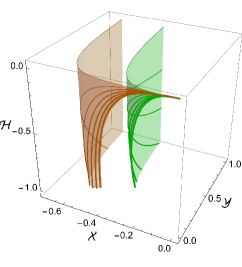
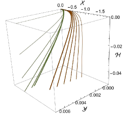
We can find exact expressions for our solutions to the system of first order differential equations (5.5)-(5.7). We subsitute expessions from (2.16)-(LABEL:g) to (5.5)-(5.7). Therefore we can present for fixed parametes of model (fixed chemical potential and temperature) solution for light and heavy quarks models in the 3D plots in $({\cal X},{\cal Y},{\cal H})$ coordinates.

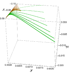
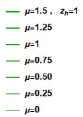
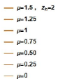
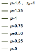
In Fig. 43 The 3D plot of $({\cal X},{\cal Y},{\cal H})$ defined by equations (5.5)-(5.7) for the light quarks model. The green lines with decreasing thickness represent the case with $z_{h}=1$ and $\mu=1.5,1.25,1,0.75,0.5,0$ . The darker orange lines represent the case with $z_{h}=2$ and the same set of $\mu$ . We see that for small values of $z$ brown and green lines almost coincides. This happens because ${\cal X}(\varphi)\to 0$ for $\varphi\to\varphi_{0}$ as in previous case for zero temperature and chemical potential. 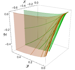This happens because (5.1) $X(z)\sim\dot{\varphi}B/\dot{B}$ , $\dot{\varphi}\to const$ and $B/\dot{B}\to 0$ for $z\to 0$ . Also ${\cal Y}$ and ${\cal H}$ $\to 0$ for $z\to 0$ .

In Fig. 44 the 3D plot $({\cal X},{\cal Y},{\cal H})$ for light quarks model is presented. The green and orange lines with decreasing thickness represent the cases with $\mu=1.5,1.25,1,0.75,0,5,0$ and different horizons $z_{h}=1$ and $z_{h}=2$ . The plot legends are the same as in Fig. 43.

b) RG flow for other solutions

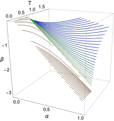
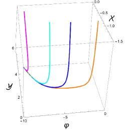
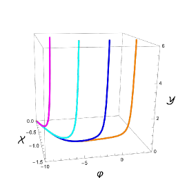
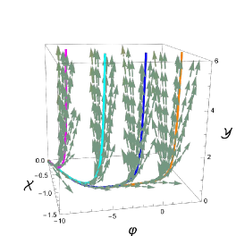
In Fig. 45A there are 3D RG plots with trajectories for fixed $z_{h}$ in $({\cal X},{\cal Y},\varphi)$ coordinates for light quarks model. These trajectories are obtained for solutions constructed from potential reconstruction method. The values of $z_{h}=0.6,2.5,4$ and $6$ correspond to magenta, cyan, blue and orange curves, respectively.

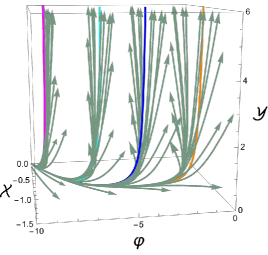
In Fig. 45B we see other solutions of RG equations (5.8),(5.9) for zero chemical potential (i.e. ${\cal H}=0$ ) for the same dilaton potential ${\cal V}(\varphi)$ . Note that solutions obtained via potential reconstruction method are unstable for light quarks model. For fixed dilaton potential ${\cal V}(\varphi)$ we solve (5.8) and (5.9) and obtain different solutions that corresponds to different factors $\mathfrak{b}(z)$ , $\varphi(z)$ and ${V}(z)$ but the same ${\cal V}(\varphi)$ . When we use reconstruction potential method we have fixed $\mathfrak{b}(z)$ , $f_{0}(z)$ and fixed boundary conditions for scalar field $\varphi$ and blackening function $g$ , and obtain only one solution of EOM. Different solutions correspond to different boundary conditions of scalar field $\varphi$ . Therefore this means that the obtained solution is sensitive to change of $\mathfrak{b}(z)$ .

5.2.2 RG flow for heavy quarks model

a) RG flow for our solution

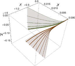
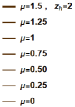
The similar plots we can present for heavy quarks model. In Fig. 46 the 3D plot of $({\cal X},{\cal Y},{\cal H})$ defined by equations (5.5)-(5.7) for the heavy quarks model. The olive lines with decreasing thickness represent the case with $z_{h}=1$ and $\mu=1.5,1.25,1,0.75,0.5,0$ . The chocolate lines represent the case with $z_{h}=2$ and the same set of $\mu$ . We can see the similar behaviour for asymptotic as for the light quarks case. Also ${\cal X}(\varphi)\to 0$ for $\varphi\to\varphi_{0}$ .

b) RG and other solutions

In Fig. 47A the 3D plots in $({\cal X},{\cal Y},\varphi)$ coordinates for heavy quarks model are presented for different boundary conditions. These boundary conditions $\varphi|_{z=z_{h}}=0$ , correspond to different values of $z_{h}=0.45,1.0,1.4$ and $1.65$ that are shown by magenta, cyan, blue and orange lines, respectively (A) and combination of our solutions in left panel with 3D RG flows in $({\cal X},{\cal Y},\varphi)$ coordinates (B).

In Fig. 47B we see other solutions of RG equations for the same dilaton potential ${\cal V}(\varphi)$ . The solutions obtained via potential reconstruction method are unstable for heavy quarks also as for light quarks case. For fixed dilaton potential ${\cal V}(\varphi)$ we solve (5.8) and (5.9) and obtain different solutions that corresponds to different factors $\mathfrak{b}(z)$ , $\varphi(z)$ and $V(z)$ but the same ${\cal V}(\varphi)$ . When we use reconstruction potential method we have fixed $\mathfrak{b}(z)$ , $f_{0}(z)$ and fixed boundary conditions for scalar field $\varphi$ and blackening function $g$ , and obtain only one solution of EOM. Therefore this means that the obtained solution is sensitive to change of $\mathfrak{b}(z)$ .

6 Conclusion and Discussion

In the paper we have considered the running coupling constant and $\beta$ -function in holographic models supported by Einstein-dilaton-Maxwell action for heavy and light quarks. We obtain a significant dependence of the running coupling constant $\alpha$ and $\beta$ -function on mass of quarks, chemical potential and temperature. At the first-order phase transitions, the functions $\alpha$ and $\beta$ functions undergo jumps depending on temperature and chemical potential. For heavy quarks these jumps depend more sharply on thermodynamic parameters. The magnitude of the jumps increases with decreasing energy scales for both light and heavy quarks.

•
The dependence of running coupling $\alpha$ for light quarks on thermodynamic parameters $\mu$ and $T$ is presented in Fig. 14. We see that
- –
  
  in the region of the hadronic phase, the running coupling increases very slowly with increasing chemical potential and temperature.
- –
  
  in the region of the QGP phase, the running coupling increases significantly faster than in the hadronic phase with increasing chemical potential and temperature.
- –
  
  the slope of increment in coupling constant is larger for lower energy scales
- –
  
  on the 1-st order transition line, the running coupling has a jump. the magnitude of the jump is zero at the CEP and increases with increasing $\mu$ near the CEP to a value that remains almost the same along the entire line of the 1-st order phase transition.
- –
  
  the magnitude of the jump increases with decreasing energy scale.
•
The dependence of running coupling $\alpha$ for heavy quarks on thermodynamic parameters $\mu$ and $T$ is presented in Fig. 21. We see that
- –
  
  in the region of the hadronic phase, the running coupling increases very slowly with increasing chemical potential and almost does not change with increasing temperature.
- –
  
  in the region of the QGP phase, the running coupling increases rather fast than the temperature increases and not so fast with increasing chemical potential.
- –
  
  the slope of increment in coupling constant is larger for lower energy scales
- –
  
  on the 1-st order transition line, the running coupling has a jump. The magnitude of the jump is greatest at $\mu=0$ and decreases along the line of the 1-st order transition to zero in the CEP.
- –
  
  the magnitude of the jump increases with decreasing energy scale.
•
The dependence of the $\beta$ -function for light quarks at a coupling constant equal to 1 on the thermodynamic parameters $\mu$ and $T$ is shown in Fig. 26. We see that
- –
  
  in all regions the $\beta$ -function is negative.
- –
  
  in the region of the hadronic phase, the $\beta$ -function is practically independent of the chemical potential and $\log|\beta|$ increases with increasing temperature.
- –
  
  in the region of the QGP phase, the $\beta$ -function increases with increasing chemical potential and decreases with increasing temperature.
- –
  
  on the 1-st order transition line, the $\beta$ -function has a jump; the magnitude of the jump is zero at the CEP and becomes negative values along the 1-st order phase transition line and takes the maximum absolute value at T=0.
- –
  
  the jump of $\log|\beta|$ decreases with increasing energy scale.
•
The dependence of the $\beta$ -function for heavy quarks at a coupling constant equal to 1 on the thermodynamic parameters $\mu$ and $T$ is shown in Fig. 33. We see that
- –
  
  in all regions the $\beta$ -function is negative.
- –
  
  in the region of the hadronic phase, the $\beta$ -function is practically independent of the chemical potential and $\log|\beta|$ increases with increasing temperature.
- –
  
  in the region of the QGP phase, the $\beta$ function increases with increasing chemical potential and decreases with increasing temperature.
- –
  
  on the 1-st order transition line, the $\beta$ -function has a jump; the magnitude of the jump is zero at the CEP and becomes negative values along the 1-st order phase transition line and takes the maximum absolute value at T=0.
- –
  
  the jump of $\log|\beta|$ decreases with increasing energy scale.
•

We also studied the RG flow near our solution. Our solution is unstable, that is inevitably associated with a negative potential, that in turn is associated with the existence of the hardonic phase.
•

The RG flow for light and heavy quarks are approximately the same although the associated warp factor is completely different.
•

Choosing different boundary conditions to obtain the RG flows for heavy and light quarks, just exert a shift in the solution without changing significantly.

It is important to note that to obtain the RG flows for heavy and light quarks we utilized some approximations for dilaton potential and gauge kinetic function. In fact, the solution of dilaton field is as a function of $z$ , i.e. $V(z)$ and gauge kinetic function $f_{0}(z)$ . Therefore, we have no direct formula for ${\cal V}(\varphi)$ and $\mathfrak{f}_{0}(\varphi)$ . Then using approximations functions, dilaton field and gauge kinetic function as a function of $\varphi$ can be obtained.

We would like to emphasize that to respect the null energy condition (NEC) we should consider the blackening function and the dilaton potential for light and heavy quarks in holographic model for different values of $\mu$ and $z_{h}$ in such a way that $z_{h}$ to be less than values of second horizon $z_{h_{2}}$ . At the second horizon $z_{h_{2}}$ temperature equals to zero. Therefore blackening function $g(z)$ should be non-negative at the interval $0\leq z\leq z_{h}$ .

Other physical quantities also have jumps at the 1-st order phase transition in isotropic and anisotropic models. Namely, entanglement entropy [63, 62], electric conductivity and direct photons emission rate [50, 64] and energy loss [66, 65] have these jumps at the 1-st order phase transition.

It is known how the primary (spatial) anisotropy affect the QCD phase transition temperature [25, 59]. Also that there is another type of anisotropy due to a magnetic field and its effect on the QCD phase diagram too, see [56, 57, 61, 49, 58, 60, 50]. The corresponding anisotropy also changes the running coupling $\alpha$ and $\beta$ -function. We will study these changes in a separate paper.

7 Acknowledgements

The work of I.A., P.S. and M.U. is supported by RNF grand 20-12–00200. The work of A.H. was performed at the Steklov International Mathematical Center and supported by the Ministry of Science and Higher Education of the Russian Federation (Agreement No.075-15-2022-265).

Appendix A EOM at zero temperature

Let us consider zero temperature case. At zero temperature the blackening function $g(z)=1$ . Then we obtain the following simplifications for the metric (2.4)

ds^{2}=\frac{e^{2A(z)}}{z^{2}}\left[-dt^{2}+d\vec{x}^{2}+dz^{2}\right]

(A.1)

and for the EOMs (2.6)-(2.10)

	$\displaystyle\varphi^{\prime\prime}+\left(3A^{\prime}-\frac{3}{z}\right)\varphi^{\prime}+\left(\frac{z^{2}e^{-2A}A^{\prime}_{t}f_{0,\varphi}}{2}-\frac{e^{2A}V_{\varphi}}{z^{2}}\right)=0,$		(A.2)
	$\displaystyle A^{\prime\prime}_{t}+\left(\frac{f^{\prime}_{0}}{f_{0}}+A^{\prime}-\frac{1}{z}\right)A^{\prime}_{t}=0,$		(A.3)
	$\displaystyle A^{\prime\prime}-A^{\prime 2}+\frac{2}{z}A^{\prime}+\frac{\varphi^{\prime 2}}{6}=0,$		(A.4)
	$\displaystyle e^{-2A}z^{2}f_{0}A_{t}^{\prime 2}=0,$		(A.5)
	$\displaystyle A^{\prime\prime}+3A^{\prime 2}-\frac{6}{z}A^{\prime}+\frac{4}{z^{2}}+\frac{e^{2A}V}{3z^{2}}=0.$		(A.6)

We see that equation (A.5) requires $A_{t}^{\prime}=0$ and we left with

	$\displaystyle\varphi^{\prime\prime}+\left(3A^{\prime}-\frac{3}{z}\right)\varphi^{\prime}-\frac{e^{2A}V_{\varphi}}{z^{2}}=0,$		(A.7)
	$\displaystyle A^{\prime\prime}-A^{\prime 2}+\frac{2}{z}A^{\prime}+\frac{\varphi^{\prime 2}}{6}=0,$		(A.8)
	$\displaystyle A^{\prime\prime}+3A^{\prime 2}-\frac{6}{z}A^{\prime}+\frac{4}{z^{2}}+\frac{e^{2A}V}{3z^{2}}=0.$		(A.9)

A.1 Preliminary about the reconstruction method

Let us consider the following action

\displaystyle S

\displaystyle=

\displaystyle\frac{1}{16\pi G_{5}}\int d^{5}x\sqrt{-g}\left[R-\frac{1}{2}\partial_{\mu}\varphi\partial^{\mu}\varphi-{\cal V}(\varphi)\right].

(A.10)

The Einstein equations that follow from the action (A.10) for the ansatz for metric (A.1) and scalar field $\varphi=\varphi(z)$ have the form

	$\displaystyle\varphi^{\prime\prime}+(3A^{\prime}-\frac{3}{z})\varphi^{\prime}-\frac{e^{2A}V_{\varphi}}{z^{2}}=0,$		(A.11)
	$\displaystyle A^{\prime\prime}-A^{\prime 2}+\frac{2}{z}A^{\prime}+\frac{\varphi^{\prime 2}}{6}=0,$		(A.12)
	$\displaystyle A^{\prime\prime}+3A^{\prime 2}-\frac{6}{z}A^{\prime}+\frac{4}{z^{2}}+\frac{e^{2A}V}{3z^{2}}=0.$		(A.13)

From equation (A.8) we get the expression for dilaton field

\displaystyle\varphi^{\prime}(z)

\displaystyle=

\displaystyle\sqrt{-6\Bigg{(}A^{\prime\prime}-A^{\prime 2}+\frac{2}{z}A^{\prime}\Bigg{)}},

(A.14)

and from equation (A.13) we get the expression for potential depending on $z$ coordinate

\displaystyle V(z)

\displaystyle=

\displaystyle-3z^{2}e^{-2A}\Bigg{[}A^{\prime\prime}+3A^{\prime 2}+\Bigg{(}-\frac{6}{z}\Bigg{)}A^{\prime}-\frac{1}{z}\Bigg{(}-\frac{4}{z}\Bigg{)}\Bigg{]}.

(A.15)

For B.C. $\varphi(z_{0})=0$ we define

\displaystyle\varphi(z,z_{0})

\displaystyle=

\displaystyle\int_{z_{0}}^{z}\sqrt{-6\Bigg{(}A^{\prime\prime}-A^{\prime 2}+\frac{2}{z}A^{\prime}\Bigg{)}}dz

(A.16)

So, our solution depends on $z_{0}$ . We can denote our solution as $\varphi_{z_{0}}(z)$ . We define

{\cal V}(\varphi,z_{0})=V\left({\cal Z}(\varphi,z_{0})\right)

(A.17)

where $V(z)$ is defined from eq.(A.15) and ${\cal Z}$ is the inverse to the function $\varphi_{z_{0}}=\varphi_{z_{0}}(z)$

{\cal Z}:\varphi\to z,\qquad\mbox{such that}\qquad\varphi_{z_{0}}({\cal Z}(\varphi_{z_{0}}))=\varphi_{z_{0}}

(A.18)

We can draw the form of ${\cal V}={\cal V}(\varphi_{z_{0}})$ using the parametric plot.

Introducing new variable

X=\frac{\dot{\varphi}}{3}\frac{B}{\dot{B}},

(A.19)

one obtains the following RG equation [19, 20]

\displaystyle\frac{d{\cal X}}{d\varphi}=-\frac{4}{3}\left(1-\frac{3}{8}{\cal X}^{2}\right)\left(1+\frac{1}{{\cal X}}\frac{\partial_{\varphi}{\cal V}(\varphi)}{{\cal V}(\varphi)}\right)

(A.20)

Now we solve equation (A.20) with boundary condition

B.C.:\qquad{\cal X}\Big{|}_{\varphi=\varphi_{1}}={\cal X}_{1}

(A.21)

We take $X=X(z)$ and solution $\varphi_{z_{0}}(z)$ with fixed $z_{0}$ and draw

{\cal X}={\cal X}(\varphi)

(A.22)

using parametric plot. Now we take some value of $\varphi=\varphi_{1}$ and in the parametric plot find ${\cal X}_{1}$

{\cal X}_{1}={\cal X}(\varphi_{1})

(A.23)

We can solve the 1-st order diff. equation (A.20) with B.C.(A.23). We denote solution ${\cal X}={\cal X}(\varphi,{\cal X}_{1},\varphi_{1})$ . Then we can find $X=X(z)$ as

X(z)={\cal X}(\varphi_{z_{0}}(z),{\cal X}_{1},\varphi_{1})

(A.24)

the result should be independent of $z_{0}$ and coincide with (A.19).

A.2 Reconstruction of the potential

A.2.1 Potential of light quarks model

Substituting the scale factor (2.15) into (2.16) and (2.19), we obtain the solution for dilaton field as

	$\displaystyle\varphi(z,\varphi_{0})=\varphi_{0}$	$\displaystyle+$	$\displaystyle 2\sqrt{3a}\left(\!\!\sqrt{2a+1}\,\mbox{arcsinh}\left(\sqrt{\frac{b(2a+1)}{3}}\,z\right)\right.$
		$\displaystyle-$	$\displaystyle\left.\sqrt{2(a-1)}\,\mathop{\mathrm{arctanh}}\nolimits\left(\sqrt{\frac{{2b(a-1)}\,}{(2a+1)bz^{2}+3}}\,z\right)\!\!\right)$

and the potential of dilaton

\displaystyle V(z)

\displaystyle=

\displaystyle-6\left(bz^{2}+1\right)^{2a-2}\left[bz^{2}\left((a(6a+7)+2)bz^{2}+5a+4\right)+2\right].

(A.26)

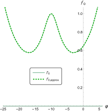
The functions $\varphi(z)$ and $V(z)$ given by (A.2.1) and (A.26) are presented in Fig. 48.A and Fig. 48.B, respectively. The function ${\cal V}(\varphi)$ that we recover from given functions $V(z)$ , eq.(A.26), and $\varphi(z)$ depending on $\varphi_{0}$ , eq.(A.2.1), is presented in Fig. 49. We see that ${\cal V}(\varphi)$ depends on $\varphi_{0}$ .

When the boundary condition for the scalar field is selected as $\varphi_{0}=-10$ at $z=0$ , we can approximate the light quarks potential function Fig. 49 by

{\cal V}_{approx,-10}(\varphi)=\sum_{i=0}^{18}c_{i}\varphi^{i},

(A.27)

and by fitting the points of the graph on the domain $-23.5\leq\varphi\leq 3.5$ , we obtain the following coefficients that is given in the Table 1 in Appendix B.

With boundary condition $\varphi_{0}=0$ at $z=0$ , the approximation for the light quarks potential takes the form

{\cal V}_{approx,0}(\varphi)=\sum_{j=0}^{18}b_{j}\varphi^{j},

(A.28)

on the domain $-13.5\leq\varphi\leq 13.5$ with fitting coefficients that is given in the Table 1 in Appendix B.

A.2.2 Potential of heavy quarks model

The solution for dilaton field by inserting the scale factor (2.24) into the expression (2.16) as

	$\displaystyle\varphi(z,\varphi_{0})=$	$\displaystyle\sqrt{6}$	$\displaystyle\int_{0}^{z}\leavevmode\nobreak\ d\xi\sqrt{\left(-4\,p\,\xi^{3}-\frac{2\,\mathrm{s}\,\xi}{3}\right)^{2}+2\left(4\,p\,\xi^{2}+\frac{2\,\mathrm{s}}{3}\right)+12\,p\,\xi^{2}+\frac{2\,\mathrm{s}}{3}}$		(A.29)
		$\displaystyle+$	$\displaystyle\varphi_{0}$		(A.29)

and the potential of dilaton

V(z)=-2\leavevmode\nobreak\ e^{\frac{1}{3}(6\,p\,z^{4}+2\,\mathrm{s}\,z^{2})}\Bigg{(}6+5\,\mathrm{s}\,z^{2}+2(9\,p+{\mathrm{s}}^{2})z^{4}+24\,p\,\mathrm{s}\,z^{6}+72\,p^{2}z^{8}\Bigg{)}.

(A.30)

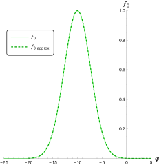
The potential of heavy quarks as a function of the scalar field is presented in Fig. 51. Considering the boundary condition for the scalar field as $\varphi_{0}=-10$ at $z=0$ , one can approximate the heavy quarks potential function Fig. 51 (khaki dashed line) by

{\cal V}_{approx,-10}(\varphi)=\sum_{i=0}^{18}\mathfrak{c}_{i}\varphi^{i},

(A.31)

and by fitting the points of the graph on the domain $-23.5\leq\varphi\leq 3.5$ , we obtain the following coefficients that is given in the Table 2 in Appendix B. Also, for choosing b.c as $\varphi_{0}=0$ at $z=0$ , one can approximate the heavy quarks potential function Fig. 51 (olive dashed line) by

{\cal V}_{approx,0}(\varphi)=\sum_{i=0}^{18}\mathfrak{b}_{i}\varphi^{i},

(A.32)

and by fitting the points of the graph on the domain $-13.5\leq\varphi\leq 13.5$ , we obtain the following coefficients that is given in the Table 2 in Appendix B. It is important to note that our valid domain in these approximations for $z$ is $-8.5\leq z\leq 8.5$ .

A.3 The blackening function $g(z)$ and the dilaton potential ${\cal V}(\varphi)$

A.3.1 Light quarks model

The blackening function and the dilaton potential depicted for the light quarks model correspondingly for different values of $\mu$ and $z_{h}$ in Fig. 52 and Fig. 53, respectively. To respect the null energy condition (NEC) we should consider holographic model for $z_{h}$ less than values second horizon $z_{h_{2}}$ . At the second horizon $z_{h_{2}}$ temperature equals to zero. Therefore blackening function $g(z)$ should be non-negative at the interval $0\leq z\leq z_{h}$ .

A.3.2 Heavy quarks model

The blackening function and the dilaton potential depicted for the heavy quarks model correspondingly for different values of $\mu$ and $z_{h}$ in Fig. 54 and Fig. 55, respectively.

A.4 Reconstruction of the gauge kinetic function $\mathfrak{f}_{0}(\varphi)$

A.4.1 Light quarks model

The gauge kinetic function for light quarks model takes the form [42]

f_{0}(z)=e^{-cz^{2}+a\log\left(bz^{2}+1\right)},

(A.33)

where the parameters $a$ , $b$ and $c$ are introduced in (2.14) and (2.15). Using the explicit form of the solution (A.2.1) in Fig. 56 we plot $\mathfrak{f}_{0}(\varphi)$ . This function can be approximated as

\mathfrak{f}_{0,approx}(\varphi)=\frac{1}{m_{3}\sqrt{2\pi}}\exp\left[-\frac{1}{2}\left(\frac{\varphi-\varphi_{0}}{m_{1}}\right)^{2}\right]+m_{2},

(A.34)

where the coefficients are the following: $m_{1}=2.70895$ , $m_{2}=8.26922*10^{-6}$ and $m_{3}=0.39931$ .

A.4.2 Heavy quarks model

The gauge kinetic function for heavy quarks takes the form [54, 43]

f_{0}(z)=e^{-\frac{2}{3}\mathrm{s}\,z^{2}+p\,z^{4}},

(A.35)

where $s$ and $p$ are the same parameters are introduced in (2.24). We utilized the form of the solution (A.29) to plot $\mathfrak{f}_{0}(\varphi)$ in Fig. 57. When the boundary condition for the scalar field is selected as $\varphi_{0}=-10$ at $z=0$ , this function can be approximated by

\mathfrak{f}_{0,approx}(\varphi)=\sum_{i=0}^{30}w_{i}\,\varphi^{i},

(A.36)

and by fitting the points of the graph on the domain $-25\leq\varphi\leq 6$ , we obtain the following coefficients that is represented in Table 3 Appendix B.

Appendix B Approximation coefficients of potential and gauge kinetic function

The coefficients of approximation of light and heavy quarks for potential function with different b.c, i.e. $\varphi_{0}=-10$ and $\varphi_{0}=0$ are given in the Table 1 and 2, respectively.

$\varphi_{0}=-10$	$\varphi_{0}=0$
$c_{0}=-8333.49$	$b_{0}=-11.996$
$c_{1}=-6769.87$	$b_{1}=-2.86057*10^{-12}$
$c_{2}=-2734.34$	$b_{2}=-1.50457$
$c_{3}=-731.531$	$b_{3}=2.544*10^{-14}$
$c_{4}=-145.923$	$b_{4}=-0.082475$
$c_{5}=-23.1662$	$b_{5}=4.19564*10^{-15}$
$c_{6}=-3.05115$	$b_{6}=-0.0020461$
$c_{7}=-0.343354$	$b_{7}=-1.87468*10^{-16}$
$c_{8}=-0.0337693$	$b_{8}=-0.0000216737$
$c_{9}=-0.00294892$	$b_{9}=3.45919*10^{-18}$
$c_{10}=-0.000229452$	$b_{10}=-2.21701*10^{-7}$
$c_{11}=-0.0000156801$	$b_{11}=-3.4441*10^{-20}$
$c_{12}=-9.12457*10^{-7}$	$b_{12}=-2.48019*10^{-10}$
$c_{13}=-4.34389*10^{-8}$	$b_{13}=1.91673*10^{-22}$
$c_{14}=-1.61884*10^{-9}$	$b_{14}=-7.31265*10^{-12}$
$c_{15}=-4.4908*10^{-11}$	$b_{15}=-5.53005*10^{-25}$
$c_{16}=-8.662*10^{-13}$	$b_{16}=1.20875*10^{-14}$
$c_{17}=-1.03328*10^{-14}$	$b_{17}=6.33555*10^{-28}$
$c_{18}=-5.74044*10^{-17}$	$b_{18}=-5.74045*10^{-17}$

Table 1: The coefficients of the approximation for light quarks potential function with two boundary condition, i.e.

\varphi_{0}=-10

and

\varphi_{0}=0

$\varphi_{0}=-10$	$\varphi_{0}=0$
$\mathfrak{c}_{0}=-22808.2$	$\mathfrak{b}_{0}=-11.9744$
$\mathfrak{c}_{1}=-21257.3$	$\mathfrak{b}_{1}=-2.20242*10^{-12}$
$\mathfrak{c}_{2}=-9781.21$	$\mathfrak{b}_{2}=-1.52795$
$\mathfrak{c}_{3}=-2964.73$	$\mathfrak{b}_{3}=-4.47153*10^{-13}$
$\mathfrak{c}_{4}=-666.91$	$\mathfrak{b}_{4}=-0.0811821$
$\mathfrak{c}_{5}=-118.904$	$\mathfrak{b}_{5}=4.56467*10^{-14}$
$\mathfrak{c}_{6}=-17.5253$	$\mathfrak{b}_{6}=-0.00460869$
$\mathfrak{c}_{7}=-2.20197$	$\mathfrak{b}_{7}=-1.74355*10^{-15}$
$\mathfrak{c}_{8}=-0.241625$	$\mathfrak{b}_{8}=-0.0000276665$
$\mathfrak{c}_{9}=-0.0235074$	$\mathfrak{b}_{9}=3.37277*10^{-17}$
$\mathfrak{c}_{10}=-0.00202414$	$\mathfrak{b}_{10}=-1.26397*10^{-6}$
$\mathfrak{c}_{11}=-0.00015091$	$\mathfrak{b}_{11}=-3.58649*10^{-19}$
$\mathfrak{c}_{12}=-9.40185*10^{-6}$	$\mathfrak{b}_{12}=4.41746*10^{-9}$
$\mathfrak{c}_{13}=-4.70369*10^{-7}$	$\mathfrak{b}_{13}=2.13034*10^{-21}$
$\mathfrak{c}_{14}=-1.81389*10^{-8}$	$\mathfrak{b}_{14}=-7.61899*10^{-11}$
$\mathfrak{c}_{15}=-5.14567*10^{-10}$	$\mathfrak{b}_{15}=-6.64785*10^{-24}$
$\mathfrak{c}_{16}=-1.00593*10^{-11}$	$\mathfrak{b}_{16}=2.05593*10^{-10}$
$\mathfrak{c}_{17}=-1.20764*10^{-13}$	$\mathfrak{b}_{17}=8.49863*10^{-27}$
$\mathfrak{c}_{18}=-6.7091*10^{-16}$	$\mathfrak{b}_{18}=-6.70907*10^{-16}$

Table 2: The coefficients of the approximation for heavy quarks potential function with two boundary condition, i.e.

\varphi_{0}=-10

and

\varphi_{0}=0

The coefficients of approximation of heavy quarks for gauge kinetic function with boundary condition $\varphi_{0}=-10$ is given in the Table 3.

$\varphi_{0}=-10$
$w_{0}=0.649979$	$w_{16}=1.31403*10^{-12}$
$w_{1}=0.0505165$	$w_{17}=6.87886*10^{-14}$
$w_{2}=0.0106962$	$w_{18}=7.47132*10^{-16}$
$w_{3}=-0.00133661$	$w_{19}=-6.25931*10^{-17}$
$w_{4}=-0.00089918$	$w_{20}=-8.64631*10^{-19}$
$w_{5}=0.000254561$	$w_{21}=1.02579*10^{-19}$
$w_{6}=0.000146991$	$w_{22}=1.07317*10^{-21}$
$w_{7}=-0.0000111608$	$w_{23}=-1.69210*10^{-22}$
$w_{8}=-0.0000108994$	$w_{24}=-1.05002*10^{-24}$
$w_{9}=-4.23684*10^{-7}$	$w_{25}=2.89729*10^{-25}$
$w_{10}=3.80199*10^{-7}$	$w_{26}=2.86221*10^{-27}$
$w_{11}=4.82338*10^{-8}$	$w_{27}=-4.96868*10^{-28}$
$w_{12}=-4.28331*10^{-9}$	$w_{28}=-2.10423*10^{-29}$
$w_{13}=-1.28932*10^{-9}$	$w_{29}=-3.46181*10^{-31}$
$w_{14}=-6.18659*10^{-11}$	$w_{30}=-2.15509*10^{-33}$
$w_{15}=8.43119*10^{-12}$

Table 3: The coefficients of the approximation of gauge kinetic function for heavy quarks with boundary condition

\varphi_{0}=-10

Appendix C Beta-function $\beta(\alpha)$ -2D plot

C.1 Beta-function $\beta(\alpha)$ for light quarks model

Beta-function $\beta=\beta(\alpha)$ for light quarks at $T=0.08$ with different $\mu$ corresponding to points in Fig. 3 and Fig. 4 is plotted in Fig. 58. The points are indicated by blue triangle $(\mu=2,\,z_{h}=0.9637)$ , two green dots $\mu=0.43,\,z_{h}=2.816$ and $\mu=0.557,\,z_{h}=3.652$ , magenta star $\mu=0.394,z_{h}=4.415$ and brown square $\mu=0.36,z_{h}=25.8$ . From Fig. 58, we see that the blue line showing $\beta(\alpha)$ for the QGP phase deviates from the linear relationship for small $\alpha$ . Also the line order (top to bottom) of the thick green and brown line changes as we move from small $\alpha$ to larger one.

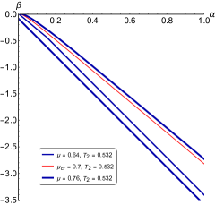
Beta-function $\beta=\beta(\alpha)$ for light quarks at $T=0.11$ with different $\mu$ corresponding to points in Fig. 3 and Fig. 4 is plotted in Fig. 59. The points are indicated by blue triangle $(\mu=2,\,z_{h}=1.0025)$ , two green dots $\mu=0.32,\,z_{h}=4.12$ and $\mu=0.557,\,z_{h}=2.5$ , magenta star $\mu=0.31,z_{h}=4.64$ and brown square $\mu=0.3,z_{h}=17.205$ . Also, for $T=0.11$ there is a linear relationship for $\beta$ as a function of $\alpha$ .

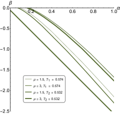
Beta-function $\beta=\beta(\alpha)$ for light quarks at different fixed $T=0.2$ , $T=0.11$ , $T=0.08$ with different $\mu$ corresponding to the points in Fig. 3 and Fig. 4 is depicted in Fig. 60. In all cases the $\beta$ -function decreases with increasing $\alpha$ .

C.2 Beta-function $\beta(\alpha)$ for heavy quark model

Beta-function $\beta=\beta(\alpha)$ for heavy quarks model at fixed $T=0.574$ , small $\mu$ (A) $T=0.532$ (B), $T=0.574$ , large $\mu$ (C) and combination of (A,B) in (D) is plotted in Fig. 61. All the lines are corresponding to the points in Fig. 9 and Fig. 10. Similar to light quark model, beta-function has the linear dependence on $\alpha$ .

In Fig. 62 the beta-function $\beta=\beta(\alpha)$ for heavy quarks model at fixed $T=0.2$ (A) $\mu=0.1$ (B), $\mu=1.5$ (C) is depicted. All lines are corresponding to the points in Fig. 9 and Fig. 10. The linear dependence of $\beta$ on $\alpha$ is also seen and increasing $\alpha$ increases the $\beta$ -function.

References

[1] N.N. Bogoliubov and D.V. Shirkov, The Theory of Quantized Fields. GTTL, Moscow (1957); English trans.: New York, NY: Interscience (1959).
[2] K. G. Wilson and J. B. Kogut, “The Renormalization group and the epsilon expansion,” Phys. Rept. 12, 75-199 (1974).
[3] Schwartz M. D. Quantum field theory and the standard model. – Cambridge university press, 2014.
[4] M. Gell-Mann, M. and F. E. Low, ”Quantum Electrodynamics at Small Distances”. Physical Review. 95 (5): 1300–1312. (1954)
[5] C. G. Callan, Jr., “Broken scale invariance in scalar field theory,” Phys. Rev. D 2, 1541-1547 (1970)
[6] K. Symanzik, “Small distance behavior in field theory and power counting,” Commun. Math. Phys. 18, 227-246 (1970)
[7] A. N. Vasil’ev, The field theoretic renormalization group in critical behavior theory and stochastic dynamics, Publishing house St. Petersburg. Institute of Nuclei. physicists (1998); English transl.: Chapman & Hall/CRC (2004)
[8] J. Zinn-Justin, Quantum field theory and critical phenomena, Oxford, Clarendon Press (2002)
[9] J. M. Maldacena, “The Large N limit of superconformal field theories and supergravity,” Adv. Theor. Math. Phys. 2, 231-252 (1998) [arXiv:hep-th/9711200 [hep-th]].
[10] J. Casalderrey-Solana, H. Liu, D. Mateos, K. Rajagopal and U. A. Wiedemann, “Gauge/String Duality, Hot QCD and Heavy Ion Collisions”, (Cambridge University Press, Cambridge, UK, 2014), [arXiv:1101.0618 [hep-th]]
[11] I. Y. Aref’eva, “Holographic approach to quark-gluon plasma in heavy ion collisions”, Phys. Usp. 57, 527-555 (2014)
[12] J. de Boer, E. P. Verlinde and H. L. Verlinde, “On the holographic renormalization group,” JHEP 08, 003 (2000) [arXiv:hep-th/9912012 [hep-th]].
[13] H. J. Boonstra, K. Skenderis and P. K. Townsend, “The domain wall / QFT correspondence,” JHEP 01, 003 (1999) [arXiv:hep-th/9807137 [hep-th]].
[14] I. Heemskerk and J. Polchinski, “Holographic and Wilsonian Renormalization Groups,” JHEP 1106 (2011) 031 doi:10.1007/JHEP06(2011)031 [arXiv:1010.1264 [hep-th]].
[15] T. Faulkner, H. Liu and M. Rangamani, Integrating out geometry: Holographic Wilsonian RG and the membrane paradigm, JHEP 1108 (2011) 051; arXiv:1010.4036.
[16] S. S. Lee, Quantum Renormalization Group and Holography, JHEP 1401 (2014) 076, arXiv:1305.3908.
[17] M. Bianchi, D. Z. Freedman and K. Skenderis, “Holographic renormalization,” Nucl. Phys. B 631, 159-194 (2002) [arXiv:hep-th/0112119 [hep-th]].
[18] K. Skenderis, “Lecture notes on holographic renormalization,” Class. Quant. Grav. 19, 5849-5876 (2002) [arXiv:hep-th/0209067 [hep-th]].
[19] U. Gursoy and E. Kiritsis, “Exploring improved holographic theories for QCD: Part I,” JHEP 02, 032 (2008) [arXiv:0707.1324 [hep-th]].
[20] U. Gursoy, E. Kiritsis and F. Nitti, “Exploring improved holographic theories for QCD: Part II”, JHEP 02, 019 (2008) [arXiv:0707.1349 [hep-th]] .
[21] E. Kiritsis, W. Li and F. Nitti, “Holographic RG flow and the Quantum Effective Action,” Fortsch. Phys. 62, 389-454 (2014) [arXiv:1401.0888 [hep-th]].
[22] E. Kiritsis, F. Nitti and L. Silva Pimenta, “Exotic RG Flows from Holography,” Fortsch. Phys. 65, no.2, 1600120 (2017) [arXiv:1611.05493 [hep-th]].
[23] U. Gürsoy, E. Kiritsis, F. Nitti and L. Silva Pimenta, “Exotic holographic RG flows at finite temperature,” JHEP 10, 173 (2018) [arXiv:1805.01769 [hep-th]].
[24] J. K. Ghosh, E. Kiritsis, F. Nitti and L. T. Witkowski, “Holographic RG flows on curved manifolds and quantum phase transitions,” JHEP 05, 034 (2018) [arXiv:1711.08462 [hep-th]].
[25] I. Aref’eva and K. Rannu, “Holographic Anisotropic Background with Confinement-Deconfinement Phase Transition,” JHEP 05, 206 (2018) [arXiv:1802.05652 [hep-th]].
[26] I. Y. Aref’eva, “Holographic Renormalization Group Flows,” Theor. Math. Phys. 200, no.3, 1313-1323 (2019)
[27] I. Y. Aref’eva and K. Rannu, “Holographic Renormalization Group Flow in Anisotropic Matter,” Theor. Math. Phys. 202, no.2, 272-283 (2020)
[28] I. Y. Aref’eva, A. A. Golubtsova and G. Policastro, “Exact holographic RG flows and the A₁ × A₁ Toda chain,” JHEP 05, 117 (2019) [arXiv:1803.06764 [hep-th]].
[29] M. Berg and H. Samtleben, “An Exact holographic RG flow between 2-d conformal fixed points,” JHEP 05, 006 (2002) [arXiv:hep-th/0112154 [hep-th]].
[30] A. A. Golubtsova and M. K. Usova, “Stability analysis of holographic RG flows in 3d supergravity,” Eur. Phys. J. Plus 138, no.3, 260 (2023) [arXiv:2208.01179 [hep-th]].
[31] K. Arkhipova, L. Astrakhantsev, N. S. Deger, A. A. Golubtsova, K. Gubarev and E. T. Musaev, “Holographic RG flows and boundary conditions in a 3D gauged supergravity,” [arXiv:2402.11586 [hep-th]].
[32] D. S. Gorbunov and V. A.Rubakov. “Introduction to the theory of the early universe: Cosmological perturbations and inflationary theory”. World Scientific, 2011.
[33] J. M. Lattimer and M. Prakash M. The equation of state of hot, dense matter and neutron stars, Phys. Rep. 621 (2016) 127-164.
[34] A. Lovato, T. Dore, R. D. Pisarski, B. Schenke, K. Chatziioannou, J. S. Read, P. Landry, P. Danielewicz, D. Lee and S. Pratt, et al. “Long Range Plan: Dense matter theory for heavy-ion collisions and neutron stars,” [arXiv:2211.02224 [nucl-th]]
[35] L. Du, A. Sorensen and M. Stephanov, “The QCD phase diagram and Beam Energy Scan physics: a theory overview,” [arXiv:2402.10183 [nucl-th]].
[36] F. R. Brown, F. P. Butler, H. Chen, N. H. Christ, Z. h. Dong, W. Schaffer, L. I. Unger and A. Vaccarino, “On the existence of a phase transition for QCD with three light quarks”, Phys. Rev. Lett. 65, 2491-2494 (1990)
[37] O. Philipsen and C. Pinke, “The $N_{f}=2$ QCD chiral phase transition with Wilson fermions at zero and imaginary chemical potential,” Phys. Rev. D 93, no.11, 114507 (2016) [arXiv:1602.06129 [hep-lat]].
[38] J. N. Guenther, “Overview of the QCD phase diagram: Recent progress from the lattice,” Eur. Phys. J. A 57, no.4, 136 (2021) [arXiv:2010.15503 [hep-lat]].
[39] G. Aarts, J. Aichelin, C. Allton, A. Athenodorou, D. Bachtis, C. Bonanno, N. Brambilla, E. Bratkovskaya, M. Bruno and M. Caselle, et al. “Phase Transitions in Particle Physics: Results and Perspectives from Lattice Quantum Chromo-Dynamics,” Prog. Part. Nucl. Phys. 133, 104070 (2023) [arXiv:2301.04382 [hep-lat]].
[40] W. j. Fu, J. M. Pawlowski and F. Rennecke, “QCD phase structure at finite temperature and density,” Phys. Rev. D 101, no.5, 054032 (2020) [arXiv:1909.02991 [hep-ph]].
[41] D. G. Dumm, J. P. Carlomagno and N. N. Scoccola, “Strong-interaction matter under extreme conditions from chiral quark models with nonlocal separable interactions,” Symmetry 13, no.1, 121 (2021) [arXiv:2101.09574 [hep-ph]].
[42] M. W. Li, Y. Yang and P. H. Yuan, “Approaching Confinement Structure for Light Quarks in a Holographic Soft Wall QCD Model,” Phys. Rev. D 96, no.6, 066013 (2017) [arXiv:1703.09184 [hep-th]].
[43] Y. Yang and P. H. Yuan, “Confinement-deconfinement phase transition for heavy quarks in a soft wall holographic QCD model,” JHEP 12, 161 (2015) [arXiv:1506.05930 [hep-th]].
[44] I. Y. Aref’eva, K. A. Rannu and P. S. Slepov, “Anisotropic solution of the holographic model of light quarks with an external magnetic field”, Theor. Math. Phys. 210, no.3, 363-367 (2022).
[45] A. Hajilou, “Meson excitation time as a probe of holographic critical point”, Eur. Phys. J. C 83, no.4, 301 (2023) [arXiv:2111.09010 [hep-th]]
[46] I. Y. Aref’eva, K. Rannu and P. Slepov, “Holographic anisotropic model for light quarks with confinement-deconfinement phase transition,” JHEP 06, 090 (2021) [arXiv:2009.05562 [hep-th]].
[47] I. Y. Aref’eva, K. Rannu and P. S. Slepov, “Anisotropic solutions for a holographic heavy-quark model with an external magnetic field”, Teor. Mat. Fiz. 207, no.1, 44-57 (2021)
[48] I. Y. Aref’eva, K. A. Rannu and P. S. Slepov, “Dense QCD in Magnetic Field”, Phys. Part. Nucl. Lett. 20 (2023) no.3, 433-437
[49] I. Y. Aref’eva, K. Rannu and P. Slepov,“Holographic model for heavy quarks in anisotropic hot dense QGP with external magnetic field,”JHEP 07, 161 (2021) [arXiv:2011.07023 [hep-th]].
[50] I. Y. Aref’eva, A. Ermakov, K. Rannu and P. Slepov, “Holographic model for light quarks in anisotropic hot dense QGP with external magnetic field,” Eur. Phys. J. C 83, no.1, 79 (2023) [arXiv:2203.12539 [hep-th]].
[51] A. Karch, E. Katz, D. T. Son and M. A. Stephanov, “Linear confinement and AdS/QCD,” Phys. Rev. D 74, 015005 (2006) [arXiv:hep-ph/0602229 [hep-ph]].
[52] S. He, M. Huang and Q. S. Yan, “Logarithmic correction in the deformed $AdS_{5}$ model to produce the heavy quark potential and QCD beta function”, Phys. Rev. D 83, 045034 (2011) [arXiv:1004.1880 [hep-ph]]
[53] H. J. Pirner and B. Galow, “Strong Equivalence of the AdS-Metric and the QCD Running Coupling”, Phys. Lett. B 679, 51-55 (2009) [arXiv:0903.2701 [hep-ph]]
[54] I. Y. Aref’eva, A. Hajilou, K. Rannu and P. Slepov, “Magnetic catalysis in holographic model with two types of anisotropy for heavy quarks,” Eur. Phys. J. C 83, no.12, 1143 (2023) [arXiv:2305.06345 [hep-th]].
[55] T. van Ritbergen, J. A. M. Vermaseren and S. A. Larin, “The Four loop beta function in quantum chromodynamics,” Phys. Lett. B 400, 379-384 (1997) [arXiv:hep-ph/9701390 [hep-ph]].
[56] U. Gursoy, M. Jarvinen and G. Nijs, “Holographic QCD in the Veneziano Limit at a Finite Magnetic Field and Chemical Potential”, Phys. Rev. Lett. 120, no.24, 242002 (2018) [arXiv:1707.00872 [hep-th]]
[57] H. Bohra, D. Dudal, A. Hajilou and S. Mahapatra, “Anisotropic string tensions and inversely magnetic catalyzed deconfinement from a dynamical AdS/QCD model”, Phys. Lett. B 801, 135184 (2020) [arXiv:1907.01852 [hep-th]]
[58] D. Dudal, A. Hajilou and S. Mahapatra, “A quenched 2-flavour Einstein–Maxwell–Dilaton gauge-gravity model”, Eur. Phys. J. A 57, no.4, 142 (2021) [arXiv:2103.01185 [hep-th]]
[59] I. Aref’eva, K. Rannu and P. Slepov, “Orientation Dependence of Confinement-Deconfinement Phase Transition in Anisotropic Media,” Phys. Lett. B 792, 470-475 (2019) [arXiv:1808.05596 [hep-th]].
[60] P. Jain, S. S. Jena and S. Mahapatra, “Holographic confining-deconfining gauge theories and entanglement measures with a magnetic field,” Phys. Rev. D 107, no.8, 086016 (2023) [arXiv:2209.15355 [hep-th]].
[61] H. Bohra, D. Dudal, A. Hajilou and S. Mahapatra, “Chiral transition in the probe approximation from an Einstein-Maxwell-dilaton gravity model,” Phys. Rev. D 103, no.8, 086021 (2021) [arXiv:2010.04578 [hep-th]].
[62] I. Y. Aref’eva, A. Patrushev and P. Slepov, “Holographic entanglement entropy in anisotropic background with confinement-deconfinement phase transition”, JHEP 07, 043 (2020) [arXiv:2003.05847 [hep-th]]
[63] D. Dudal and S. Mahapatra, “Interplay between the holographic QCD phase diagram and entanglement entropy”, JHEP 07, 120 (2018) [arXiv:1805.02938 [hep-th]]
[64] I. Y. Aref’eva, A. Ermakov and P. Slepov, “Direct photons emission rate and electric conductivity in twice anisotropic QGP holographic model with first-order phase transition”, Eur. Phys. J. C 82, no.1, 85 (2022) [arXiv:2104.14582 [hep-th]]
[65] I. Y. Aref’eva, K. A. Rannu and P. S. Slepov, “Spatial Wilson loops in a fully anisotropic model”, Teor. Mat. Fiz. 206, no.3, 400-409 (2021)
[66] I. Y. Aref’eva, K. Rannu and P. Slepov, “Energy Loss in Holographic Anisotropic Model for Heavy Quarks in External Magnetic Field”, [arXiv:2012.05758 [hep-th]]