Enhancing Rolling Horizon Production Planning Through Stochastic Optimization Evaluated by Means of Simulation

Abstract

Production planning must account for uncertainty in a production system, arising from fluctuating demand forecasts. Therefore, this article focuses on the integration of updated customer demand into the rolling horizon planning cycle. We use scenario-based stochastic programming to solve capacitated lot sizing problems under stochastic demand in a rolling horizon environment. This environment is replicated using a discrete event simulation-optimization framework, where the optimization problem is periodically solved, leveraging the latest demand information to continually adjust the production plan. We evaluate the stochastic optimization approach and compare its performance to solving a deterministic lot sizing model, using expected demand figures as input, as well as to standard Material Requirements Planning (MRP). In the simulation study, we analyze three different customer behaviors related to forecasting, along with four levels of shop load, within a multi-item and multi-stage production system. We test a range of significant parameter values for the three planning methods and compute the overall costs to benchmark them. The results show that the production plans obtained by MRP are outperformed by deterministic and stochastic optimization. Particularly, when facing tight resource restrictions and rising uncertainty in customer demand, the use of stochastic optimization becomes preferable compared to deterministic optimization.

1 Introduction

Fluctuating demand forecasts complicate supply chain management in various industrial sectors necessitating advanced production planning to mitigate customer-driven uncertainty. In these highly dynamic environments, effectively using mathematical optimization for medium-term production planning and control (PPC) requires the adoption of rolling horizon planning and the regular incorporation of updated planning data, such as customer demand, inventory levels, or available capacity. Albeit, medium-term PPC can be performed by solving deterministic or stochastic mathematical optimization models, in industry often simple algorithmic medium-term planning approaches, such as material requirements planning (MRP), are applied. Stochastic optimization is a particularly well-suited approach in dynamic settings, as it adeptly incorporates uncertainties into the decision-making process.

Customer demand constitutes externally sourced information that exhibits fluctuations over time, particularly within the framework of supply chain networks. Their digitalization promotes periodic exchange of demand information between the supply chain partners, i.e. between supplier (manufacturer) and customer in form of demand forecasts. In the context of production systems, it is typical for customers to provide long-term demand forecasts. These forecasts are regularly adjusted to ensure precise anticipation of their needs, a practice often referred to as forecast evolution and necessitates dynamically adjusting production plans based on evolving forecasts (Heath and Jackson 1994).

A suitable concept to implement the described problem domain in one application framework is the combination of discrete-event simulation with a solver for the optimization problem. Simulation provides a controlled environment for assessing various production strategies and their potential outcomes before operational implementation, which enhances decision-making and resource utilization. Simulation can be used to model diverse production system-relevant probabilistic behaviors like changing demand and shop floor related uncertainties. This allows to test the suitability of production schedules in the face of changing operational conditions and helps to increase the overall efficiency and performance of manufacturing systems (Sahin, Narayanan, and Robinson 2013).

This article’s central focus is to evaluate rolling horizon planning via solving stochastic capacitated lot sizing problems as a medium-term planning strategy in a dynamic context by means of simulation. Determining optimal lot sizing decisions ensures efficient utilization of resources, such as labor, machinery, and raw materials. This becomes critical in uncertain environments where customer demands change over time and shop floor processing underlies stochasticity, for instance caused by stochastic setup times. To tackle these issues, a simulation-optimization framework is introduced, combining discrete-event simulation with two-stage stochastic programming in a rolling horizon environment. The goal of the simulation-optimization framework is to minimize the overall costs in a multi-item and multi-stage production system. This includes costs associated with setup, production, inventory and backlog. The effectiveness of this framework is assessed through a comprehensive simulation study. The available literature on the integration of simulation and optimization has shown that it is a viable method for systematically examining and addressing the complexities of real-world production systems.

One the one hand, the simulation component provides an accurate and up-to-date representation of the production system over the entire simulation run time, including all types of stochastic influences. One the other hand, the optimization component repeatedly solves a capacitated lot sizing problem that does not replicate the full spectrum of stochasticity, based on the most current production system status. Even though not all stochastic aspects, e.g. shop floor uncertainties, can be considered within the optimization component, the dynamic interaction with the simulation component allows to mitigate stochastic effects on the production system. Additionally, considering a part of the stochastic parameters, e.g. uncertain customer demands, in the optimization model should further reduce the overall stochastic impacts.

Other researchers already demonstrated the potential of simulation-optimization for medium-term planning. In Gansterer, Almeder, and Hartl (2014) simulation-optimization is utilized to determine good planning parameters for MRP under four distinct demand scenarios. In Almeder, Gansterer, and Hartl (2009) discrete-event simulation and optimization are combined to identify an operation plan for a supply chain network based on a case study. In Forel and Grunow (2023) rolling-horizon planning and forecasting are integrated into a capacitated lot-sizing formulation and numerical results are computed using simulation. The mentioned articles are closely related to our work, but several aspects are different from our research: in our work, customer demands are generated by the forecast evolution approach for each planning period (day) and are continuously updated along the planning horizon until the due date is reached. This enables an in-depth investigation of rolling horizon planning updates per due date on the underlying multi-item and multi-stage production system. Simulation provides the basis for the comparison between production plans obtained by solving capacitated lot-sizing problems and those obtained by applying standard MRP. It offers insights into the competitiveness of the optimization results, indicating their potential effectiveness. In this article we perform a simulation-based performance comparison benchmarking deterministic and two-stage stochastic optimization against standard MRP. We use MRP as the baseline since it is the defacto industry standard for hierarchical PPC, and still subject to active research. In our implementation, to ensure optimal planning outcomes, optimization problems are consistently solved to optimality throughout the entire simulation runtime.

To systematically evaluate the performance of the proposed simulation-optimization framework, we use an elementary multi-item and multi-stage production system comprising two end items, each consisting of one component. The exemplary production system allows to analyze the effects of frequent demand updates on the performed rolling horizon planning decisions. To increase the complexity of the studied production system, we consider three different customer behaviors and uncertainty on the shop floor expressed by demand fluctuations and stochastic setup times. We also compare four different shop floor loads to analyze the planning behavior under congestion on the shop floor. Finally, the aspect of suitable planning parameter selection is addressed as they strongly influence the planning results.

This article’s theoretical contributions are threefold: firstly, it introduces a comprehensive event-based simulation framework that integrates forecast evolution, medium-term planning, scheduling and shop floor processing. Secondly, the framework supports dynamic, real-time interaction among components throughout the simulation workflow, and enables comprehensive configuration of planning and simulation parameters through an integrated database module. Thirdly, it offers a performance comparison between MRP and deterministic/stochastic optimization under varying shop loads and demand uncertainty levels, allowing to derive important managerial insights. For instance, in production environments characterized by low resource utilization and accurately predictable customer demands, standard MRP is a sufficient planning method. In situations where capacity is tight or demands underlie some uncertainty, MRP is however not competitive with production plans obtained by solving an optimization model.

The remainder of this article is structured as follows: Section 2 provides a literature review on research activities centered around the simulation-optimization approach in production planning. Section 3 introduces the components of the developed simulation-optimization framework, explaining how medium-term planning, short-term planning, and shop floor processing interact. Subsequently, Section 4 describes the context of the simulation study, including details about the production system and the experimental setup. In Section 5, the numerical results are presented and discussed. Finally, Section 6 concludes with a summary and an outlook on possible future research activities.

2 Literature Review

In this section we review works that combine simulation and optimization in order to solve difficult decision problems in the production industry, especially lot sizing. Several works consider single-item production environments, e.g. Campuzano-Bolarín et al. (2020) investigate variable lead times for a single-item single-echelon system. They evaluate lot sizing techniques, namely Silver-Meal and Wagner-Within, in a system dynamics simulation and propose a rolling horizon planning approach. Also Vargas and Metters (2011) study rolling horizon planning for a one product uncapacitated master scheduling problem under stochastic demand. They show that explicitly considering demand stochasticity within the lot sizing model is superior to adding safety stocks in terms of costs.

The case of several items is considered in Brandimarte (2006), where a plant-location-based lot sizing formulation for multi-item single-echelon production systems under multi-stage demand uncertainty is proposed. The production plans obtained by solving the stochastic models are compared to the results of a deterministic model. The respective production decisions are applied in a rolling horizon manner. Within the simulation, customer demand is assumed to follow a normal distribution and respectively scenario trees are sampled according to this assumption. Multiple production stages and demand updates, as they are used within our work, are not considered.

Gansterer, Almeder, and Hartl (2014) present different approaches to efficiently determine important MRP parameters as they are used in hierarchical production planning, namely planned lead time, safety stock and lot sizes. After analyzing a regular grid over the possible parameter settings in order to find the most suitable setting, they apply a variable neighborhood search procedure to find the best setting in a shorter amount of time. While this work exclusively focuses on planning by means of MRP with well chosen parameters, we additionally solve mathematical lot sizing models and investigate the obtained production plans.

Several medium-term planning approaches aim at additionally including short-term decisions within the planning procedure. One example is the integrated lot sizing and scheduling problem, which is studied in Curcio et al. (2018). Detailed scheduling decisions are taken into account in the optimization model. The authors investigate static robust and two-stage stochastic optimization approaches as approximation strategies to the multi-stage setting. Customer demand is assumed to follow a log-normal distribution. The integrated lot sizing and cutting stock problem under demand uncertainty is studied in Curcio et al. (2022). The authors apply a robust and two-stage stochastic optimization approach in a rolling horizon manner, in order to adapt the models to the multi-stage stochastic setting. However, including short term decisions within the medium term planning model leads to a strong increase in model size and makes it more difficult to obtain a solution quickly.

Quezada et al. (2020) consider multi-stage stochastic programming for an uncapacitated remanufacturing environment. Among other parameters, customer demand is assumed to be uncertain. Scenario trees are used to represent this uncertainty and demands are sampled from a uniform distribution. The authors develop a branch and cut algorithm and apply the proposed multi-stage stochastic model in a rolling horizon manner. Capacity restrictions are not considered, even though they constitute a major limitation in real-world environments. For this reason we investigate a capacitated setting and analyze the effect of different resource utilizations.

Simonis and Nickel (2023) investigate simulation-optimization for tablet production in the pharmaceutical industry. In this work, optimization is not applied in a rolling horizon setting. Instead, the authors solve the lot sizing problem for the full planning horizon, simulate the obtained production plan, use the simulation results to update the optimization model and start over the next optimization run. This is done until the optimization result does not change anymore. Customer demand is assumed to be uncertain and a variable neighborhood search procedure to solve the lot sizing problem in a generalized uncertainty framework is proposed.

The forecast evolution model is considered in the work of Forel and Grunow (2023). They study the differences of using the additive and multiplicative version of forecast evolution in dynamic lot sizing under demand uncertainty. In their approach the authors investigate a multi-stage demand uncertainty setting, however modify the model by splitting the time horizon in two parts. A piecewise-linear approximation is used to determine production lots in the short term, whereas a scenario-tree representation is used to model the demand uncertainty for the later periods. Instead of focusing on different variants of the forecast evolution modeling approach, we analyze different customer update behaviours in combination with varying levels of resource utilization and investigate the suitability of three planning strategies.

Almeder, Gansterer, and Hartl (2009) investigate simulation and optimization in a supply chain network context. They consider several suppliers, production facilities and customers, while modelling the material flow via different transportation modes. In their work optimization and simulation are applied iteratively, each considering a different level of details, using mixed integer linear programming (MILP) models to obtain decision rules for a discrete-event simulation environment. The authors point out, that with this approach it is possible to treat nonlinearities, complex structures, stochasticity in the simulation environment, while the optimization is able to provide optimal solutions for a simplified version of the problem. In our work, we also follow this idea, however, instead of exclusively using deterministic optimization models, we also make use of stochastic models. This allows us to explicitly consider future demand variations in the planning procedure.

For a broad overview of the full spectrum of simulation-optimization methods we refer to available survey papers, such as Figueira and Almada-Lobo (2014). The authors explore the characteristics of the different approaches and provide a systematic classification and taxonomy. Also Juan et al. (2015) review literature that combines optimization techniques with simulation in order to make better decisions in uncertain real world environments. For general literature on the lot sizing problem we refer to the comprehensive surveys of Karimi, Fatemi Ghomi, and Wilson (2003), Jans and Degraeve (2008) and Quadt and Kuhn (2008).

Even though mathematical optimization models for lot sizing problems have already been applied to stochastic demand situations in a rolling horizon setting, to the best of our knowledge, we are the first to investigate different customer update behaviours and system utilizations. This allows to derive important managerial insights regarding the suitability of different planning approaches. Moreover, we evaluate the proposed planning strategies not only by drawing random demand realizations, but by using discrete-event simulation. This allows to consider additional uncertainties on the shop floor, such as stochastic setup times, in the planning procedure.

3 Simulation-optimization framework

To assess the performance of MRP against deterministic/stochastic optimization, a numerical study was carried out. This section will detail the elements of the created simulation model starting with demand generation using forecast evolution, followed by the implemented planning approaches, namely MRP, as well as the used deterministic and stochastic optimization models and finally, how these components interact during a simulation run.

3.1 Forecast evolution model

To evaluate the influence of customer demand on a production system, it is effective to use a range of varying customer demand scenarios. In a typical supply chain setting, customers provide and regularly update long-term demand forecasts. An effective method to assess the impact of these varying forecast uncertainties is to generate customer demand using the additive Martingale Model of Forecast Evolution (MMFE) method (Heath and Jackson 1994; Norouzi and Uzsoy 2014).

For the applied MMFE the variable $D_{itb}$ in Equation (1) denotes the demand forecast for item $i$ for due date $t$, which is provided $b$ periods before delivery. The variable $F_{it}$ represents the long-term forecast of end item $i$ for due date $t$. This is a constant model parameter for end items and set in a way that the expected order amount $E[D_{it0}]$ is for example 200 units. The forecast update horizon, denoted by $T$, is the period during which forecast updates are performed. For periods beyond the forecast horizon $t>T$, customers provide the long-term forecast $F_{it}$. Within the applied simulation model for $T$ the constant value of ${{12}}$ periods is set.

$${D_{itb}}=\left\{\begin{array}[]{ll}{F_{it}}&\text{for }b>T\\ {{F_{it}}+{\varepsilon_{itb}}}&\text{for }b=T\\ {D_{it,b+1}+{\varepsilon_{itb}}}&\text{for }b<T\\ \end{array}\right.$$ (1)

The random update term applied during $b\leq T$ is denoted as $\varepsilon_{itb}$ in Equation (2). This $\varepsilon_{itb}$ is modelled as a truncated normally distributed random variable with mean $0$ and a standard deviation $\sigma_{\varepsilon}$, which is defined as the $\alpha$ fraction of the long-term forecast $F_{it}$. In this setting, $\alpha$ represents the level of unsystematic forecast error. The unsystematic forecast error is the unpredictable, random deviation in forecasting outcomes (Zeiml et al. 2019; Altendorfer and Felberbauer 2023). Note that for the forecast updates $\varepsilon_{itb}$, a truncated normal distribution is necessary to avoid negative demand forecast values, i.e., $\varepsilon_{itb}>(-D_{it,b+1})$ and $\varepsilon_{itb}<D_{it,b+1}$. Setting $\varepsilon_{it0}=0$ indicates the final order amount, with no more updates in the delivery period. The expected order amount $E[D_{it0}]$ is set to the corresponding demand scenarios quantities for the end items in the numerical study.

$${\varepsilon_{itb}}\sim N\left({0,{\sigma_{\varepsilon}}}\right);{\rm{}}{\sigma_{\varepsilon}}=\alpha{F_{it}}$$ (2)

In the numerical study, different values for $\alpha$ are tested, in combination with three different customer behaviors, in order to evaluate their influence on the planning results. More detailed information on the investigated customer behaviours can be found in Section 4.2.

3.2 Material Requirements Planning (MRP)

Medium-term planning is part of hierarchical production planning and involves making decisions that have a significant impact on the overall production capacity and the allocation of resources over a duration of several weeks or months (Luo, Thevenin, and Dolgui 2022). The medium-term planning approach of MRP provides detailed material replenishment and capacity plans to cover a planning horizon extending over a few months (Dolgui and Prodhon 2007). Advantage of standard MRP is the algorithmic simplicity of iteratively repeating steps, which always provides an applicable production plan independent of the production system complexity. One disadvantage of standard MRP is the missing capacity limitation for a planning period due to the decoupling of the time-phasing procedure (which relies on fixed planned lead times) from the time-dependent workloads in individual departments (Zijm and Buitenhek 1996). From a manufacturing perspective, this leads to plans, which may be infeasible due to missing machine capacity. MRP is also prone to the bullwhip effect due to planning nervousness introduced by changes in the Master Production Schedule (MPS) (Rahman, Rahman, and Talapatra 2020). The concept of MRP is known for its textbook description like Hopp and Spearman (2011), Orlicky (1975) or Vollmann, Berry, and Whybark (1997) using tables and detailed verbal descriptions of the according steps. In contrast Segerstedt (1996) and Bregni et al. (2013) are representing MRP in mathematical terms. Regardless of its formalization, MRP is an approach aimed at finding planning solutions that effectively align both internal and external supply and demand, while explicitly taking into consideration the lead times involved. The primary objective is to keep the projected inventory levels low for end items and components within the planning horizon, based on the selected lot-sizing policy. MRP additionally ensures that the projected inventory on hand remains above or equal to the established safety stock level. There also exist further developments of MRP like the concept of demand driven MRP (DDMRP), which enhances the traditional MRP approach to better handle dynamic demand and supply chain variability. The core idea of MRP, however, remains the same (Ptak and Smith 2018). The following procedure describes standard MRP as it is implemented in our discrete-event simulation model. At the beginning, all customer demands that fall within the predetermined planning horizon are considered as part of the standard MRP process. From an algorithmic perspective, the process of MRP involves the following steps: (i) The gross requirements are applied to perform netting, (ii) The predetermined lot sizing policies ”fixed order quantity” (FOQ) or ”fixed order period” (FOP) are applied, (iii) Time phasing is done, typically through backward scheduling with fixed planned lead times, (iv) The gross requirements for necessary components and raw materials are calculated through the bill of materials (BOM) explosion step. These steps are executed for the specified items in the BOM, starting with the end items that have a low level code (LLC) of 0, and progressing until the final LLC is reached. The work of Hopp and Spearman (2011) provides detailed information on standard MRP, and the simulation framework was implemented accordingly.

3.3 Optimization models

In this paper, next to standard MRP, we also obtain production plans by formulating and solving MILP models, which we integrate into the developed simulation-optimization framework. Our models are based on the multi-item multi-echelon capacitated lot sizing formulations of Thevenin, Adulyasak, and Cordeau (2021). Table 1 provides the necessary notation.

Index set	Definition
$t,\tau\in\mathcal{H}=\{1,\ldots,T\}$	Planning horizon
$i,j\in\mathcal{I}=\mathcal{I}_{e}\cup\mathcal{I}_{c}$	Items
$\mathcal{I}_{c}=\{1,\ldots,M\}$	Components
$\mathcal{I}_{e}=\{{M\!+\!1},\ldots,{M\!+\!N}\}$	End items
$k\in\mathcal{K}=\{1,\ldots,J\}$	Resources
$\mathcal{K}_{i}$ for $i\in\mathcal{I}$	Resources that are needed to produce item $i$
$\mathcal{I}_{k}$ for $k\in\mathcal{K}$	Items that are produced on resource $k$
$\omega\in\Omega$	Set of scenarios
Parameter	Definition
$D_{it}$	Demand of end item $i$ in period $t$
$\hat{I}_{i0}$	Initial inventory of item $i$
$\hat{I}_{it}$	Arriving production order of item $i$ in period $t$
$R_{ij}$	Number of units of item $i$ needed for 1 unit of $j$ (BOM)
$L_{i}$	Lead time of item $i$
$C_{kt}$	Capacity of resource $k$ in period $t$
$s_{ik}$	Setup cost of item $i$ for resource $k$
$t_{ik}$	Setup time of item $i$ for resource $k$
$p_{ik}$	Production time of item $i$ for resource $k$
$v_{i}$	Production cost of item $i$
$h_{i}$	Holding cost of item $i$
$b_{i}$	Backlog cost of end item $i$
$e_{i}$	Lost sales cost of end item $i$ (backlog at period $T$)

Table 1: Problem parameters

The task is to produce a set of items $\mathcal{I}$ over a fixed discrete time horizon $\mathcal{H}$, using capacitated production resources $\mathcal{K}$, in order to satisfy customer demand for these items, which underlies some uncertainty. The goal is to minimize the total costs, consisting of setup, production, inventory, backlog and lost sales costs. Items can be separated into end items $\mathcal{I}_{e}$, that face external customer demand, and components $\mathcal{I}_{c}$ that are needed for the production of end items, as well as other components. The operation structure is represented by the BOM $R_{ij}$, defining the number of units of component $i$ necessary to produce one unit of item $j$. Each item $i\in\mathcal{I}$ has a lead time $L_{i}$ that needs to pass, before it can be further processed. In order to produce an item $i$, all necessary resources $\mathcal{K}_{i}$ need to be set up. For each of these resources $k$ the setup procedure comes at a setup cost of $s_{ik}$ and consumes a setup time of $t_{ik}$ units of the $C_{kt}$ units that are available in period $t$. Furthermore each produced unit of item $i$ comes at production cost $v_{i}$ and consumes additional production time $p_{ik}$ of resource $k$. At the beginning of the planning horizon there are $\hat{I}_{i0}$ units of item $i$ available in the initial inventory. During the planning horizon, in each period $t$ arriving production orders $\hat{I}_{it}$ of item $i$ may become available. These orders have been started in earlier periods before the start of the planning horizon and can be used for further processing, as soon as they arrive. Production capacity that is occupied by these arriving orders is already excluded from the available capacity $C_{kt}$. In each period of the planning horizon $\mathcal{H}$ there is customer demand for end items $\mathcal{I}_{e}$, which underlies some uncertainty. Demand of a certain period can either be satisfied by items that are on inventory or items that are finished in the respective period. Storing items on inventory comes at holding costs $h_{i}$. In the case where not enough items are available to satisfy the demand, backlog costs $b_{i}$ per period need to be paid until the demand is fulfilled. Backlog not satisfied in the last period of the planning horizon is considered as lost sales. These cannot be fulfilled later and incur lost sales costs $e_{i}$, which are usually much higher than backlog costs. Allowing lost sales guarantees a feasible solution, even in the case where the production capacity is not sufficient to fulfill all customer orders during the planning horizon. The task is to determine setups and production quantities, that define a production plan respecting the requirements of the operation structure and production system, while minimizing the total resulting costs.

3.3.1 The deterministic optimization model

Despite the fact, that the underlying production environment faces several uncertainties, such as stochastic customer demands and setup times, it is reasonable to solve a deterministic optimization model at every stage of the rolling horizon setting. Due to frequent updates that the optimization part receives from the simulation environment, the relevant information adapts over time. Decisions made in the deterministic model are based on the latest available information update, without considering possible changes in the future. Table 2 shows the variables used in the deterministic optimization model, which is formulated in (3) - (11).

Variable	Definition
$Y_{it}$	Binary setup variable of item $i$ in period $t$
$Q_{it}$	Production quantity of item $i$ in period $t$
$I_{it}$	Inventory of item $i$ in period $t$
$B_{it}$	Backlog of end item $i$ in period $t$

Table 2: Deterministic model variables

$$\min\sum_{i\in\mathcal{I}_{e}\cup\mathcal{I}_{c}}\sum_{t\in\mathcal{H}}\left(\sum_{k\in\mathcal{K}_{i}}s_{ik}Y_{it}+v_{i}Q_{it}+h_{i}I_{it}\right)+\sum_{i\in\mathcal{I}_{e}}\left(\sum_{t=1}^{t=T-1}b_{i}B_{it}+e_{i}B_{iT}\right)$$ (3)

such that

$$\sum_{\tau=1}^{t-L_{i}}Q_{i\tau}+\hat{I}_{i0}+\sum_{\tau=1}^{t}\hat{I}_{i\tau}-\sum_{\tau=1}^{t}D_{i\tau}-I_{it}+B_{it} =0 i\in\mathcal{I}_{e},t\in\mathcal{H}$$ (4)

$$\sum_{\tau=1}^{t-L_{i}}Q_{i\tau}+\hat{I}_{i0}+\sum_{\tau=1}^{t}\hat{I}_{i\tau}-\sum_{\tau=1}^{t}\sum_{j\in\mathcal{I}_{e}\cup\mathcal{I}_{c}}R_{ij}Q_{j\tau}-I_{it} =0 i\in\mathcal{I}_{c},t\in\mathcal{H}$$ (5)

$$Q_{it} \leq M_{it}Y_{it} i\in\mathcal{I},t\in\mathcal{H}$$ (6)

$$\sum_{i\in\mathcal{I}_{k}}t_{ik}Y_{it}+p_{ik}Q_{it} \leq C_{kt} t\in\mathcal{H},k\in\mathcal{K}$$ (7)

$$Y_{it} \in\{0,1\} i\in\mathcal{I},t\in\mathcal{H}$$ (8)

$$Q_{it} \geq 0 i\in\mathcal{I},t\in\mathcal{H}$$ (9)

$$I_{it} \geq 0 i\in\mathcal{I},t\in\mathcal{H}$$ (10)

$$B_{it} \geq 0 i\in\mathcal{I}_{e},t\in\mathcal{H}$$ (11)

The objective (3) is to minimize the total costs over the planning horizon, which consist of setup, production, inventory, backlog, and lost sales costs. While production and inventory costs incur for all items, backlog costs only incur for end items. Backlog in the last period of the planning horizon is denoted separately as lost sales. Constraints (4) and (5) define the inventory balance for end items and components respectively, taking into account lead times. Constraints (6) make sure that items can only be produced if the suitable setup is made in the respective period. The capacity constraints (7) restrict the combined consumption of resource capacity by setup time and production time for each period and resource. Finally, the variable domains are specified in (8) - (11).

3.3.2 The stochastic optimization model

Although due to frequent updates, uncertainty in the parameters can be partly considered in a rolling horizon style deterministic optimization, it still comes with several disadvantages. Production lots are connected via several production stages, which respectively have certain lead times. In order to effectively consider uncertainty in the customer demands, fluctuations need to be anticipated long before the actual due date. Reaction times in production systems with several echelons are usually longer than one period, meaning that a demand update shortly before the actual due date cannot be compensated anymore by updated optimization runs. The used mathematical model should make use of the available information on the parameter’s stochasticity at every call. To realize this, a suitable approach is two-stage scenario-based stochastic optimization, see e.g. Birge and Louveaux (2011). It takes into account the stochasticity by sampling discrete scenarios from an assumed underlying probability distribution and incorporating a metric over these scenarios, such as the expected value, into the optimization model. In the following, we denote a scenario by $\omega$ and corresponding demand realization as $D_{it}^{\omega}$, which represents the realized demand of end item $i\in\mathcal{I}_{e}$ in period $t\in\mathcal{H}$ for scenario $\omega$. The set of all scenarios included in the optimization model is denoted as $\Omega$, with the number of scenarios being the cardinality $|\Omega|$ of this set. Within the optimization model each scenario $\omega$ is weighted with a probability of $p_{\omega}$. In the following, we describe a stochastic version of the model presented in Section 3.3.1, using two-stage scenario-based stochastic programming. In two-stage models decision variables are split into first stage and second stage decisions. While first stage decisions are fixed before the uncertainty is realized, second stage decisions can be adjusted after the uncertain parameters are revealed. Decisions variables of the first stage can be implemented here-and-now, while variables of the second stage are scenario dependent and are therefore referred to as wait-and-see decisions. In order to be able to derive production orders from the solution of the stochastic optimization model, we define setup and production quantity decisions as first stage variables, while inventory and backlog variables form the second stage decisions. The latter depend on the realization of the scenarios and are therefore equipped with an additional scenario index $\omega$. Table 3 shows the used decision variables for the stochastic model, which is further formulated in (12)-(16).

Variable	Definition
$Y_{it}$	Binary setup variable of item $i$ in period $t$
$Q_{it}$	Production quantity of item $i$ in period $t$
$I_{it}^{\omega}$	Inventory of item $i$ in period $t$ for scenario $\omega$
$B_{it}^{\omega}$	Backlog of end item $i$ in period $t$ for scenario $\omega$

Table 3: Stochastic model: variables

$$\min \sum_{i\in\mathcal{I}_{e}\cup\mathcal{I}_{c}}\sum_{t\in\mathcal{H}}\left(\sum_{k\in\mathcal{K}_{i}}s_{ik}Y_{it}+v_{i}Q_{it}\right)$$ (12)

$$+\sum_{\omega\in\Omega}p_{\omega}\left(\sum_{i\in\mathcal{I}_{e}\cup\mathcal{I}_{c}}\sum_{t\in\mathcal{H}}h_{i}I_{it}^{\omega}+\sum_{i\in\mathcal{I}_{e}}\left(\sum_{t=1}^{t=T-1}b_{i}B_{it}^{\omega}+e_{i}B_{iT}^{\omega}\right)\right)$$

such that

$$\eqref{deterministic_setup_constraint},\eqref{deterministic_capacity_contraint},\eqref{deterministic_domain_setup},\eqref{deterministic_domain_quantity}$$

$$\sum_{\tau=1}^{t-L_{i}}Q_{i\tau}+\hat{I}_{i0}+\sum_{\tau=1}^{t}\hat{I}_{i\tau}-\sum_{\tau=1}^{t}D_{i\tau}^{\omega}-I_{it}^{\omega}+B_{it}^{\omega} =0 i\in\mathcal{I}_{e},t\in\mathcal{H},{\omega\in\Omega}$$ (13)

$$\sum_{\tau=1}^{t-L_{i}}Q_{i\tau}+\hat{I}_{i0}+\sum_{\tau=1}^{t}\hat{I}_{i\tau}-\sum_{\tau=1}^{t}\sum_{j\in\mathcal{I}_{e}\cup\mathcal{I}_{c}}R_{ij}Q_{j\tau}^{\omega}-I_{it}^{\omega} =0 i\in\mathcal{I}_{c},t\in\mathcal{H},{\omega\in\Omega}$$ (14)

$$I_{it}^{\omega} \geq 0 i\in\mathcal{I},t\in\mathcal{H},\omega\in\Omega$$ (15)

$$B_{it}^{\omega} \geq 0 i\in\mathcal{I}_{e},t\in\mathcal{H},\omega\in\Omega$$ (16)

The objective (12) of the stochastic optimization model is to minimize the total resulting costs over the planning horizon consisting of setup and production costs, as well as the expected inventory, backlog and lost sales costs over all scenarios $\omega\in\Omega$. Setup and resource capacity constraints (6) and (7) remain unchanged from the deterministic model. The inventory balance for end items and components need to hold for all scenarios $\omega\in\Omega$ and are transformed to (13) and (14). While variable domains (8) and (9) for setups and quantities remain unchanged, the domains for inventory and backlog variables are modified to (15) and (16).

3.4 Simulation-optimization framework development

In this section, we introduce the developed simulation-optimization framework and elaborate on the interaction of its technical components. In general, discrete-event simulation stands as a well-established approach for modeling production systems, enabling the exploration and enhancement of performance across various system configurations (Altendorfer, Felberbauer, and Jodlbauer 2016; Altendorfer and Felberbauer 2023; Enns 2001; Juan et al. 2015). It can be used to mimic the behavior of a production system for a time-span of up to several years relying on a hierarchical planning approach like MRP (Seiringer et al. 2022; Werth et al. 2023), reorder points system (RPS) (Seiringer, Altendorfer, and Felberbauer 2023), constant work in progress (CONWIP) (Xanthopoulos and Koulouriotis 2021), or in combination with an MILP model to plan production (Gansterer, Almeder, and Hartl 2014). To effectively integrate production system simulation with optimization in a rolling horizon planning framework, several key requirements need to be addressed. On the one hand, up-to-date system and demand related information needs to be provided to the optimization component by the simulation environment. This information comprises the latest customer demand updates, available inventory and production orders currently being processed, as well as occupied resource capacities. On the other hand, the output of the optimization results, e.g. the optimal decision variables, need to be utilized to create production orders which can subsequently be processed in the simulation environment. In the following, the most important planning and interaction requirements are described in more detail.

3.4.1 Planning and interaction requirements

Rolling horizon planning is dynamic, involving several critical steps. The process begins by starting the simulation application with a limited runtime of $n$ periods. During the simulation, a rolling horizon planning window, which captures a timespan of $T$ periods from the current simulation time $\bar{t}$, is iteratively shifted by one discrete time period. In this context $T$ denotes the length of the planning window. A shift of the rolling horizon window is performed by moving the observed interval from $(\bar{t},\bar{t}+T)$ to $(\bar{t}+1,\bar{t}+1+T)$. We will also refer to this shift as the beginning of a new planning cycle. This procedure is done until the current simulation time $\bar{t}$ is equal to the runtime limit $n$.

After a new planning cycle has started, new customer orders are generated and existing orders are updated according to the forecast evolution model outlined in Section 3.1. The demand forecast of an order for item $i$ and due date $t$ is denoted by $D_{itb}$, assuming that the current simulation time is $b$ periods before the due date, i.e. $t-\bar{t}=b$. After generating and updating customer demands, the simulation provides two types of parameters to the optimization component. First, general information on the production system setting is required. This comprises information on the components $\mathcal{I}_{c}$ and end items $\mathcal{I}_{e}$, as well as resources $\mathcal{K}$ and respective resource requirements of items ($\mathcal{I}_{k}$ and $\mathcal{K}_{i}$). Furthermore, BOM structure ${R}_{ij}$ and time related parameters, e.g. lead times ${L}_{i}$, setup times ${t}_{ik}$ and processing times ${p}_{ik}$, need to be provided. Finally, also cost-related parameters, e.g. setup ${s}_{ik}$, processing ${v}_{i}$, holding ${h}_{i}$, backlog ${b}_{i}$ and lost sales costs ${e}_{i}$, are part of the required general information and need to be passed to the optimization component. These parameters stay constant during the whole simulation runtime.

Next to the general information, the optimization component also requires dynamic parameters that change during simulation. These include the inventory at hand $\hat{I}_{i0}$ and information on arriving orders during the planning window $\hat{I}_{it}$, as well as available resource capacity ${C}_{kt}$ and finally, the updated customer demand forecasts ${D}_{itb}$. To provide the initial inventory $\hat{I}_{i0}$, the current on stock quantity of item $i$ at the current simulation time is reported. To identify the production orders $\hat{I}_{it}$ of item $i$ that will arrive in period $t$, all waiting and processing orders with planned end $t$ are selected and the respective order quantities are summed. To compute the available capacity ${C}_{kt}$ of a resource $k$ in period $t$ all planned and running production orders in the simulation are selected and their required capacity is subtracted from the initially available capacity of the upcoming period. For currently running production orders (at time $\bar{t}$), only the remaining capacity requirement between the current simulation time and the planned end date is taken into consideration. For waiting production orders, the full requirement is subtracted. In case that the summed capacity requirement of the production orders in the simulation exceeds the full capacity of a resource in the upcoming period, capacity of the subsequent periods is consumed, meaning that $C_{kt}$ is reduced respectively. Finally, the latest demand information for customer orders within the planning horizon is provided to the optimization component. Depending on the optimization approach, different parameters are necessary. For the deterministic optimization model it is sufficient to report the most recent demand forecasts $D_{itb}$, which are used as the deterministic demands $D_{it}$ in the model. The scenario-based stochastic optimization on the other hand, makes use of different scenarios $\omega\in\Omega$ and the respective scenario demands $D_{it}^{\omega}$ to generate production plans that perform well in the face of uncertain customer demand. In order to generate meaningful demand scenarios, we use historical demand forecasts $D_{it^{\prime}b}$, where the due date $t^{\prime}$ was already prior to the current simulation time $\bar{t}$, i.e. $t^{\prime}<\bar{t}$, to estimate how much the actually realized demand at the due date will differ from its prediction. For this reason, we look at each customer order and the respective end item to see how the predicted quantity compares to the actual quantity when the order is due and track this deviation during the whole demand information horizon. We collect these deviations during the warm-up phase $z$ of the simulation, i.e. $0\leq\bar{t}\leq z$, and calculate the mean deviation for each combination of end item $i$ and distance to due date $b$. For all of these combinations this allows us to estimate the standard deviation $\sigma_{ib}$ of a truncated normal distribution, which is later used to draw the scenario demands $D_{it}^{\omega}$ for the stochastic optimization model. Assuming that the due date $t$ is reached in $b$ periods, the respective mean of the truncated normal distribution is modeled as the most current prediction $D_{itb}$, which represents the most up-to-date information available. To summarize, the scenario demands $D_{it}^{\omega}$ for end item $i$ at due date $t$ used in the stochastic optimization model are drawn from a truncated normal distribution with mean $D_{itb}$ and standard deviation $\sigma_{ib}$, assuming that period $t$ is $b$ periods from the current simulation time. For a more detailed explanation of this procedure we refer to Altendorfer and Felberbauer (2023)

After all necessary general and dynamic parameters are provided to the optimization component, the chosen model can be formulated and solved. The simulation environment is required to await the resolution of the optimization problem. After solving the model to optimality, the optimization component returns the optimal decision variables, e.g. the production quantities ${Q}_{it}$ to the simulation. Production quantities having a period index corresponding to the current simulation time $\bar{t}$ are used to generate production orders in the simulation, e.g. for $Q_{it}=200$, a production order of 200 pieces for item $i$ is generated if $t=\bar{t}$. These production orders are released immediately at time $\bar{t}$, i.e. the planned start date is $\bar{t}$. The end date of each created production order of item $i$ is set to the sum of the planned start date and the respective planned lead time $L_{i}$. Finally, the orders are released and processed on the shop floor, where the released production orders of previous periods are processed as well. The current period is simulated until the beginning of the next discrete period, which triggers the next planning cycle. In the following section the technical interaction of the developed components is described in more detail.

3.4.2 Simulation-optimization component interaction

The simulation model is provided in form of a discrete-event simulation model developed with Anylogic. In Figure 1 a schematic representation of the simulation-optimization framework is shown.

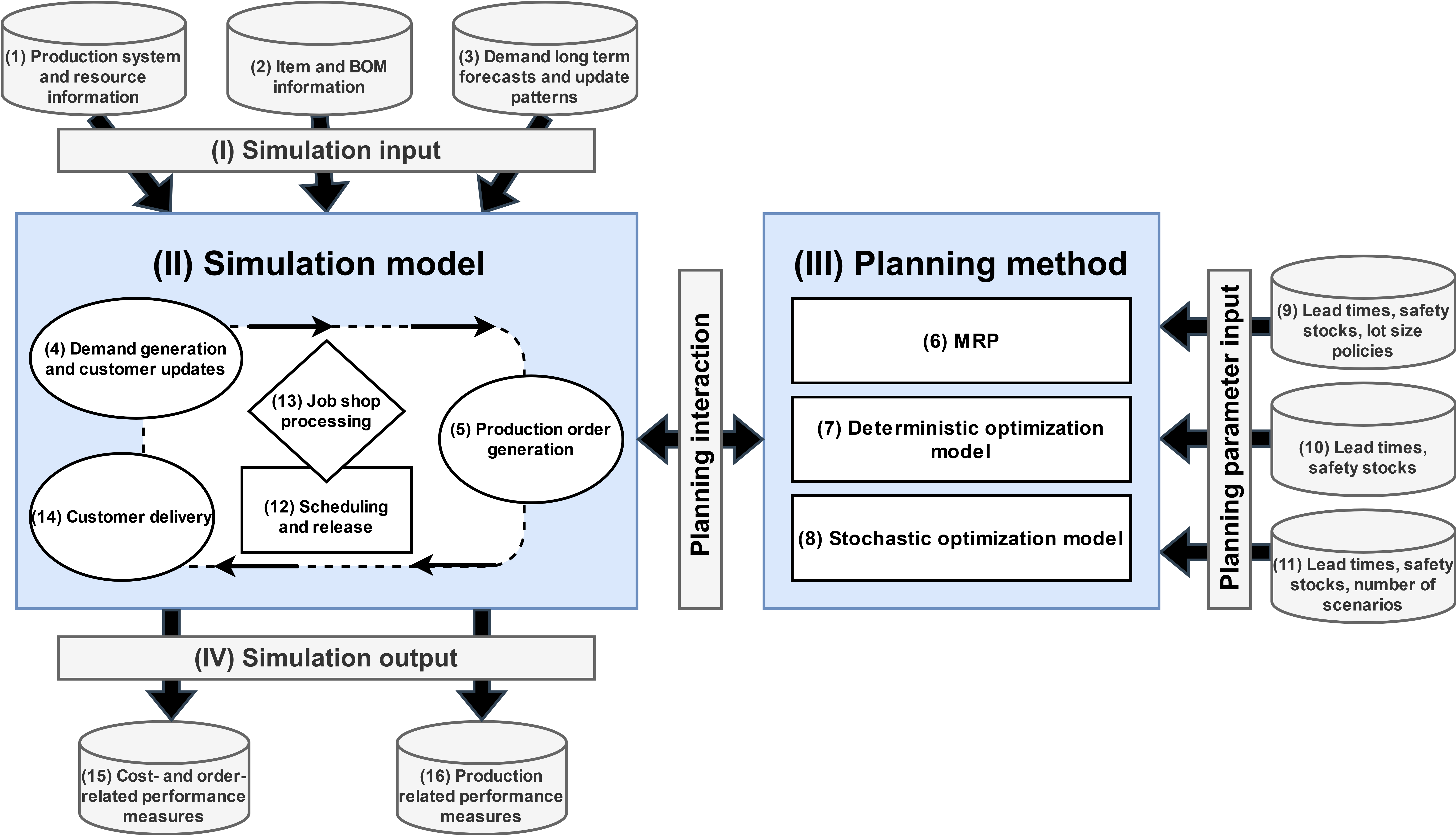
Figure 1: Component interaction of simulation-optimization framework

The four main components are simulation input (I), simulation model (II), planning method (III) and simulation output (IV). This is also the order in which the components are interacting. First the simulation input is provided to the simulation model which iteratively calls the planning method and finally stores the simulation output in a relational database, after the simulation run is finished. The simulation input comprises three types of input data:

1. Production system information concerning available resources and their respective capacities.

2. BOM and routing information, specifying which resources are required to processes the items.

3. Customer demand information, including long-term forecasts, as well as frequency and level of demand updates.

A more detailed description of the required demand forecast information is presented in Section 4.2. After the input data are available, the simulation model (II) simulates the production system until the end of the defined simulation runtime $n$. This requires the repeated call of the simulation components. First, the demand generation and customer update (4) component periodically generates the customer orders with the relevant information of item, quantity and due date. In this component the forecast evolution described in Section 3.1 is implemented. The production order generation (5) component is called to generate production orders based on the input of a chosen planning method (III). The production order generation component can be seen as the interface for the planning interaction between the simulation model (II) and the planning method (III). In our framework, three planning methods are available, among which one is selected to be applied per simulation scenario. MRP (6) is implemented in Anylogic directly, whereas, the deterministic optimization model (7) and the stochastic optimization model (8) are implemented in python, which uses CPLEX as MIP-solver. The python code is called from Anylogic during the simulation run and the simulation waits until the result is returned by the python module. For each of these three planning methods, the parameters lead time and safety stock must be defined, see the numbers (9), (10) and (11) in Figure 1. For MRP, also one of the lot sizing policies, either FOP or FOQ, must be set before running the simulation. For the stochastic optimization model, also the number of scenarios is provided. Independent of the planning method, the computed release plan is used by the production order generation component to create new orders in the simulation. These orders are subsequently passed to the scheduling and release (12) component. The production orders are sorted according to earliest due date (EDD) and are released to the corresponding machine queue. Their processing is then simulated in the job shop processing component (13). The respective amount of items of a finished production order are put on stock immediately after being finished and are available for customer delivery (14). Finished components are available for further processing of end items on the shop floor. To assess the service level, we check the difference between the due date of a customer order and its actual delivery. Delayed orders are fulfilled as soon as the required amount of items is available in stock. Finally, the simulation model provides two types of output. On the one hand, there are cost- and order related key performance indicators (KPI), such as inventory-, tardiness or overall costs over the whole simulation run per time unit [TU]. On the other hand, production related performance measures like utilization per machine or actual release dates of production orders are reported.

4 Simulation study setup

The simulation study aims at comparing the performance of MRP to deterministic and stochastic optimization in a rolling horizon planning environment. For this purpose the above described KPIs are computed. Lost sales costs are used in the optimization model to guarantee feasibility of production plans in every situation. To ensure meaningful evaluation, each replication of the simulation ran for $n=400$ periods (equivalent to days), with the first 40 periods serving as a warm-up phase, i.e. $z=40$. After the warm-up phase, all statistics were reset, assuming that the simulation systems reached a steady state. This setting allowed an investigation of the production planning approach over the course of one year, considering a daily planning frequency.

Two sources of uncertainty were considered in the simulation. Firstly, uncertainty was introduced into the forecasting process for customer demand. Secondly, stochastic setup times were simulated assuming a log-normal distribution. The log-normal distribution is often used in production systems due to its positive skewness and ability to model variables with a lower limit of zero and large positive values. Its multiplicative nature simplifies analysis when dealing with variables that result from the multiplication of independent factors (Limpert and Stahel 2017). The processing time of items and components, however, was assumed to be deterministic, assuming a stable production process. To capture the stochastic effects, 10 replications were used for each iteration. An iteration corresponds to a completed simulation run for the predetermined runtime of $n$ periods.

In the following, the evaluated production system including the planning parameters, demand and shop loads are introduced. In Section 4.2, the tested forecast scenarios are listed. We consider planned shop loads at the levels of: 85%, 90%, 95%, and 98%. These shop load levels are determined based on the set processing time. They allow a meaningful investigation of the production system behavior and represent realistic scenarios. A lower shop load than 85% will only marginally reflect effects of the tested planning parameters. For production companies, the economic target is also a high system shop load to reduce costs for production downtimes. The 98% shop load level is particularly interesting as it allows us to observe how the production system responds to tardiness caused by stochastic effects.

4.1 Production system

The evaluated production system is illustrated in Figure 2. Albeit the BOM consists of only three levels, it allows a meaningful comparison of optimization and MRP in the context of rolling horizon planning with forecast related demand uncertainty and production planning related performance indicators like tardiness, WIP level and inventory. It is important to recognize that smaller systems provide a clearer understanding of how planning parameter settings, influence outcomes (Vidal, Coronado-Hernández, and Minnaard 2022). The end items $10$ and $11$, at low-level-code (LLC) $0$ are produced on machine M2. The components $20$ and $21$ are produced on machine M1. For one unit of end item $10$, we need $1$ unit of component $20$. Likewise, we need $1$ piece of component $21$ for final product $11$. The raw material $100$, which is a purchased product, is needed for the components $20$ and $21$. This raw material is assumed to be always available and no stock out can occur for it.

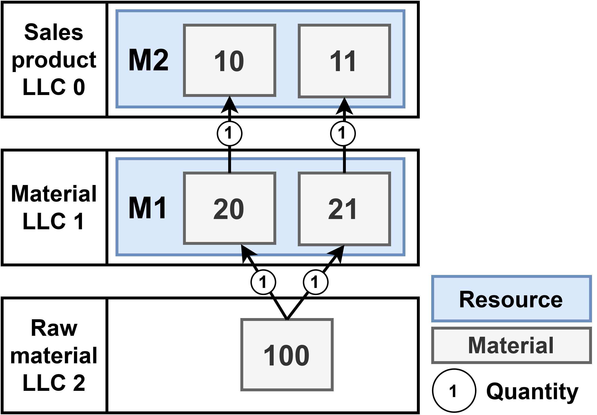
Figure 2: A 3-level BOM for our stochastic MRP example.

For the production system, a base demand scenario has been established, in which customers consistently order on average 200 units of item 10 and 400 units of item 11 each period (day). This baseline demand scenario is diversified by incorporating various customer behaviors, as detailed in Section 4.2, which enable a comparative analysis of these behaviors and their impact on production system performance. To compute planned shop loads of 85%, 90%, 95% and 98% for the demand scenario, the following settings are used: end item and component processing times in minutes per shop load are 1.56 minutes for 85%, 1.68 minutes for 90%, 1.8 minutes for 95% and 1.872 minutes for 98%. For all items a setup time of 144 minutes is applied. The value of 144 is based on a period capacity of 1440 minutes and a setup proportion of 10%. To parameterize the applied log-normal distribution for setup time, the coefficent of variance (CoV) is set to 20% leading to 28.8 minutes. This makes the production system capable of producing 600 unites per period (day). In the deterministic case, applying MRP, without forecast updates and a fixed setup time, with lot sizing policy FOP set to 1 and a planned lead time of 1 period, the planned shop load e.g. 98% is reached with service level 100%. These settings reflect the aimed at production system behavior of one setup in every planning period.

4.2 Customer types and demand parameters

As introduced in Section 3.1, we model the uncertain behaviour of customer demand via the forecast evolution model. By varying the frequency of demand updates, their magnitude and respective distance to the due date, different demand behaviours can be modeled. In our numerical experiment, we study three customer behaviours. Customer A represents a very reliable customer that only once changes the long-term forecast with the beginning of the demand information horizon when $T$ is 12. Afterwards no further updates are submitted by customer A. This mimics a deterministic demand setting for the optimization model, since there are no demand updates within the planning horizon. Customer B, on the other hand, can only give a brief estimation of the required amount in advance at the beginning of the demand information horizon, when $T$ is 12. The actual demands at the due dates can however vary significantly from the first submitted demand estimation, which is modelled by a second demand update right before the respective due date. Finally, Customer C changes demand information frequently and updates the required amount in every period of the planning horizon. Since the same $\alpha$-values are applied for Customer B and Customer C, the demand update pattern of Customer C represents the highest uncertainty among the three investigated customer types.

Furthermore, we study different demand variation factors $\alpha$. Variation factors represent the percentage of the long-term forecast by which the demand changes at every demand update step. The higher these $\alpha$ values are, the more demand uncertainty has to be absorbed by the production system. In our numerical experiment, we vary $\alpha$ within the range {0.025, 0.05, 0.075, 0.1, 0.125}, meaning that demands are changed between 2.5% and 12.5% of the long-term forecast at every update step. Through the analysis of these customer behaviors, our objective is to explore the managerial significance of demand information. This includes evaluating the impact of receiving daily updates on demand changes (or demand updates every period), the consequences of having a stable forecast but an uncertain demand realization (or only receiving a single update at the due date), and understanding the effects of the demand variation factor on decision-making processes.

4.3 Planning parameters

In addition to customer types and demand variation factors, planning parameters for MRP and parameters for both deterministic and stochastic optimization are evaluated. Parameter ranges for this evaluation were chosen based on preliminary simulations.

For MRP, the parameters include safety stock (SS), lot policies such as fixed order period (FOP) with a number of periods (NP), fixed order quantity (FOQ) with lot size (LS), and planned lead time (LT). The ranges for SS are multiples of 0, 0.1, 0.2, 0.3, 0.4, 0.5, and 0.6 of the long-term forecast for the end item. For example, for item 10 with a forecast of 200 units, the safety stock (SS) range would be 0, 20, 40, 60, 80, 100, and 120 units. For FOP the NP values considered are 1, 2, 3, 4 and 5 and LT is set to 1, 2, 3 and 4 periods. For FOQ a LS is set at multiples of 0.5, 1.0, 1.25, 1.5, 1.75, and 2 times the long-term forecast. For example, for item 10 with a forecast of 200 units, the LS values would be 100, 200, 250, 300, 350, and 400 units.

These values are also applied to the components associated with the end items in the (BOM). Selecting the same planning parameters for both end items and components is a suitable approach and allows a focused performance analysis of MRP in comparison to deterministic and stochastic optimization methods. In total, this results in 50,400 different MRP parameterizations, including the three customer types and demand parameters.

For deterministic and stochastic optimization, LT values of 1, 2, and 3 are evaluated, with SS values matching those in MRP. In stochastic optimization, the number of scenarios tested are 10, 20, 30, 50, 70, and 100. This leads to 1,260 different parameterizations for deterministic optimization and 7,560 for stochastic optimization. Each parameterization is simulated with 10 replications, resulting in a total of 592,200 individual simulation runs (MRP: 50,400; deterministic optimization: 1,260; stochastic optimization: 7,560).

5 Numerical results

In this section, we present the results from the simulation study conducted to compare standard MRP against deterministic and stochastic optimization approaches. The discussed results represent the overall costs in cost units (CU) per period computed by the sum of finished goods inventory (FGI), Work in Progress (WIP) and tardiness per unit. For end items a FGI costing factor of 2 is applied, for the associated WIP a value of 1. The inventory holding costs for components are 1 and for components WIP they are 0.5. Tardiness costs for the end items is set to 38. The relation of end items WIP and end item tardiness costs represents a target service level of 95%. A service level of 0.95 means there is a 95% chance that the inventory on hand will satisfy customer needs, thereby eliminating the risk of running out of stock. The inventory costs of end items and components are twice the WIP value, as it is more costly to store end items or components. In the subsequent sections, we begin by presenting the baseline MRP results under medium demand variation ($\alpha=7.5\%$), which serve as reference values for benchmarking against deterministic and stochastic optimization. This is followed by an exploration of a suitable number of scenarios for the stochastic optimization model. Subsequent sections delve into the effects of shop load congestion and the impact of forecast uncertainty. The final section provides a comprehensive overview of costs and parameter variations across different resource utilizations, customer demand patterns, and levels of demand variation.

5.1 MRP baseline

The well established medium-term planning approach of MRP is widely applied in industry and therefore serves as a benchmark. While the MRP data presented in Figure 3 does not introduce novel MRP-specific discoveries, they do offer valuable perspectives on planning outcomes and validate the accuracy of the MRP simulation. Within Figure 3, the minimum MRP overall costs associated with the simulated shop loads are illustrated. Each curve symbolizes distinct customer behaviors (reliable Customer A, volatile Customer B, nervous Customer C) subjected to a medium demand variation of 7.5%. Based on these behaviors, Customer A, characterized by the least uncertainty, invariably results in the lowest overall costs across all shop loads. The increasing demand uncertainty for Customers B and C corresponds to a noticeable increase in overall costs for every shop load. Meanwhile, the regular demand adjustments attributed to Customer C inject the highest unpredictability into the production system, culminating in the most pronounced overall costs across all shop loads.

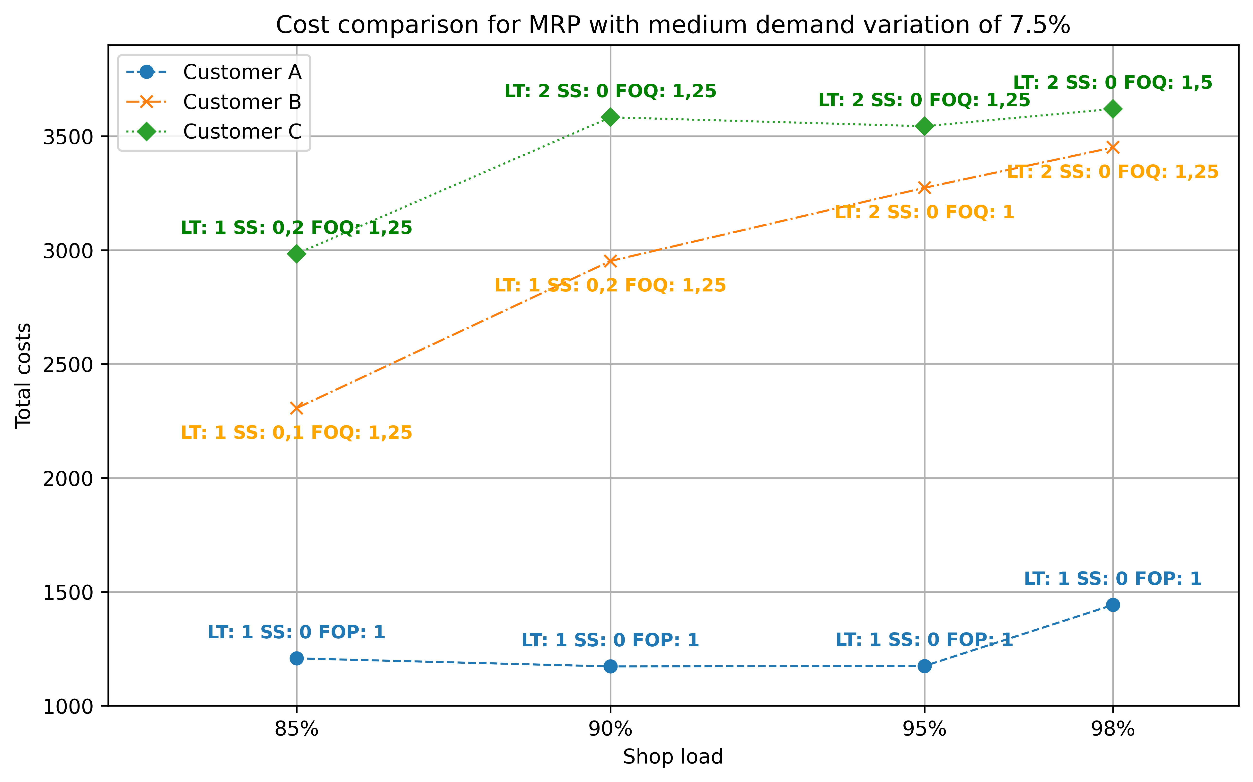
Figure 3: MRP baseline

The optimal planning parameters for Customer A, which result in the minimum total costs, have been identified as LT (Lead Time) $=1$, SS (Safety Stock) $=0$, and FOP (Fixed Order Period) $=1$. This strategy is effective due to Customer A’s deterministic demand behavior, which enables the production system to counteract stochastic effects without needing safety stock, and by utilizing the minimum values for LT and FOP. However, when the shop load reaches $98\%$, there is a slight increase in overall costs, as the higher production lead time causes increased tardiness within the production system.

For Customer B, characterized by volatile demand, employing FOQ consistently results in the minimum overall costs, effectively mitigating the impact of a higher shop load. Specifically, at shop loads of $85\%$ and $90\%$, the most cost-effective approach involves a modest safety stock combined with LT $=1$ and FOQ $=1.25\%$. At higher shop loads of $95\%$ and $98\%$, the best planning performance is achieved by increasing the lead time to 2 periods instead of using safety stock.

A similar trend is observed for the nervous Customer C. For a shop load of $85\%$, combining a lead time of 1 with safety stock attains the lowest overall costs. For higher shop loads, however, it is more effective to replace safety stock with an increased lead time.

In conclusion, these identified parameter combinations are meaningful from a production logistics perspective. For reliable Customer A, with its largely deterministic demand, minor variations from the long-term forecast can still be efficiently managed within a lead time of 1, without safety stock, and by adopting a lot-for-lot approach as indicated by FOP 1. Similarly, for Customers B and C, who exhibit more volatile and fluctuating demand patterns, meaningful planning parameters are employed. The higher shop load necessitates compensation through either a safety stock or a longer lead time. An increased lead time helps avoid production delays caused by larger lot sizes, while a small safety stock can effectively buffer against demand fluctuations.

5.2 Exploring a suitable number of scenarios for the stochastic optimization model

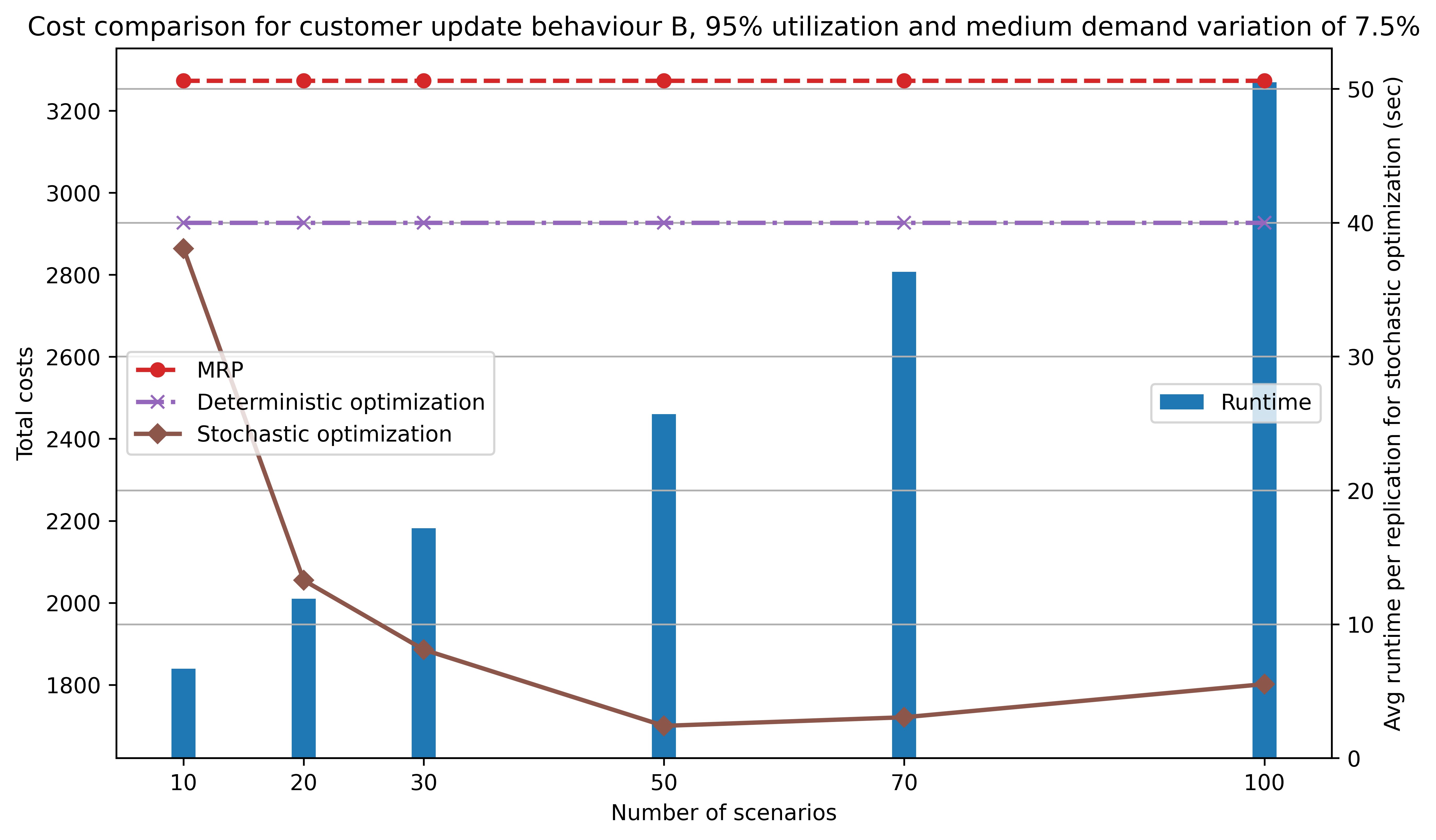
Figure 8: Number of scenarios evaluation for customer pattern B

A relevant parameter for the stochastic optimization model, introduced in Section 3.3.2, is the number of demand scenarios included in the model. Including more scenarios leads to a better approximation of the stochastic demand distribution and should therefore provide a better performance of the approach. On the other hand, including more scenarios also negatively impacts the time required to solve the stochastic optimization model. Within this section we aim at finding a reasonable number of scenarios to include in our stochastic model and perform experiments with the number of scenarios in {10,20,30,50,70,100}. We evaluate the case of nervous customer update behaviour C with a medium demand variation of 7.5% in a production environment with 95% utilization. Figure 4 shows the obtained total costs of the stochastic optimization model for an increasing number of included scenarios. Despite the fact that the performance of the deterministic model, as well as MRP are independent of the number of included scenarios, we report their performance in the investigated setting to put the stochastic performance into perspective. Additionally, on a second y-axis we report the average runtime of the stochastic optimization model for one replication using the respective number of included scenarios. We see a strong improvement in total costs when including 20 instead of 10 scenarios, for which the stochastic approach performs worse than the deterministic model. Increasing the number of scenarios to 30 further reduces the costs, however the improvement is significantly smaller. The runtime has increased from 6 seconds for 10 scenarios to 17 seconds for 30 scenarios. While the inclusion of further scenarios only results in slight cost reductions it significantly increases the average runtime for solving the stochastic models. For this reason we have decided to include 30 scenarios in all following stochastic models, which serves as a reasonable trade-off between solution quality and runtime. In the Appendix, we also report the results for demand update pattern B in Figure 8, which supports our choice.

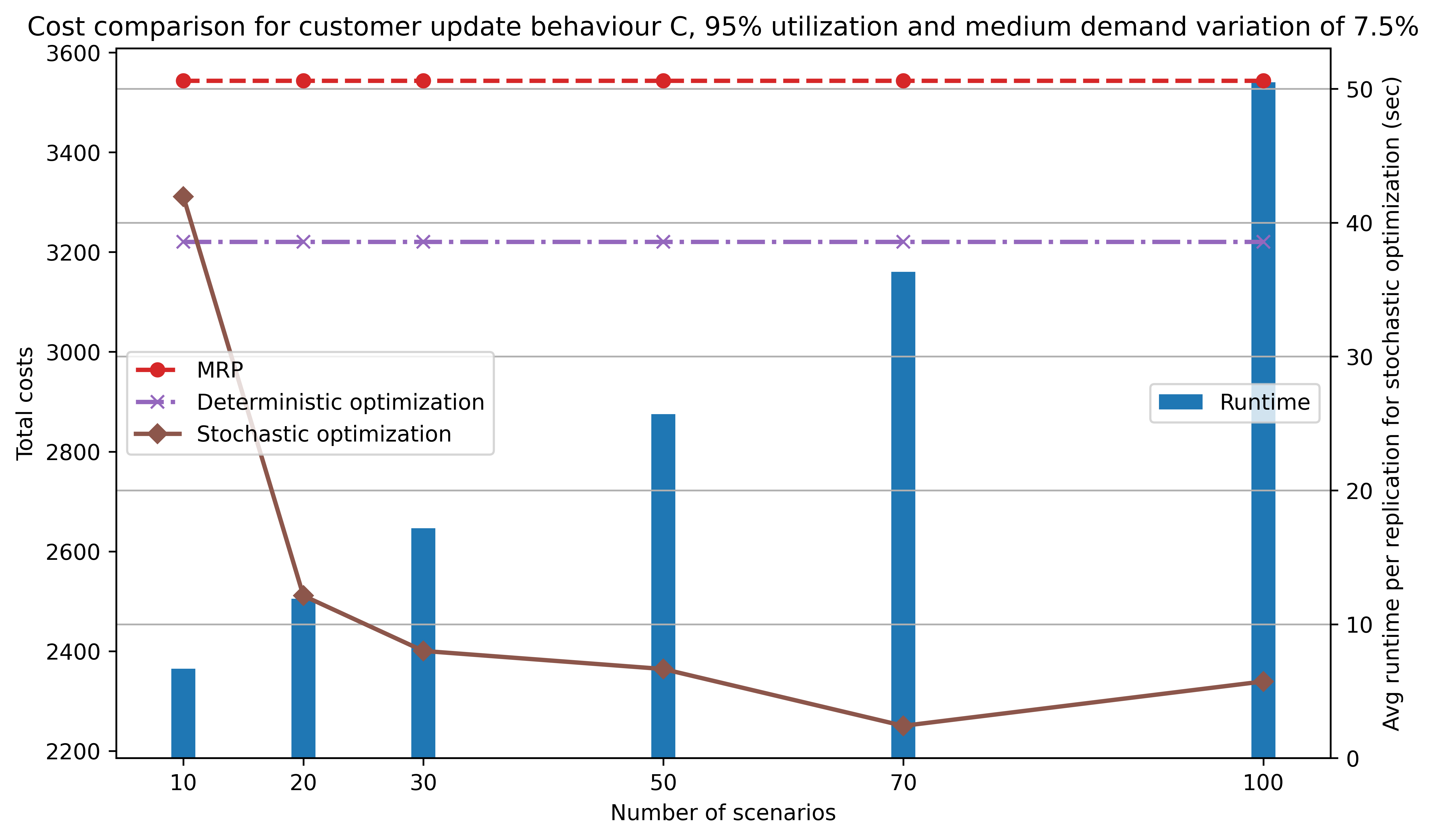
Figure 4: Number of scenarios evaluation for customer pattern C

5.3 The impact of shop load congestion

In this section, we study the effects of an increased shop load, which possibly leads to congestion on the shop floor. We report the cost reduction of deterministic and stochastic optimization models over standard MRP for customers A, B and C in the case of medium demand variation (7.5%) and resource utilizations of 85%, 90%, 95% and 98%. For each of the three planning approaches we use the best performing parameter combination. The results are displayed in Figure 5 for the deterministic, while Figure 6 shows the results for the stochastic approach.

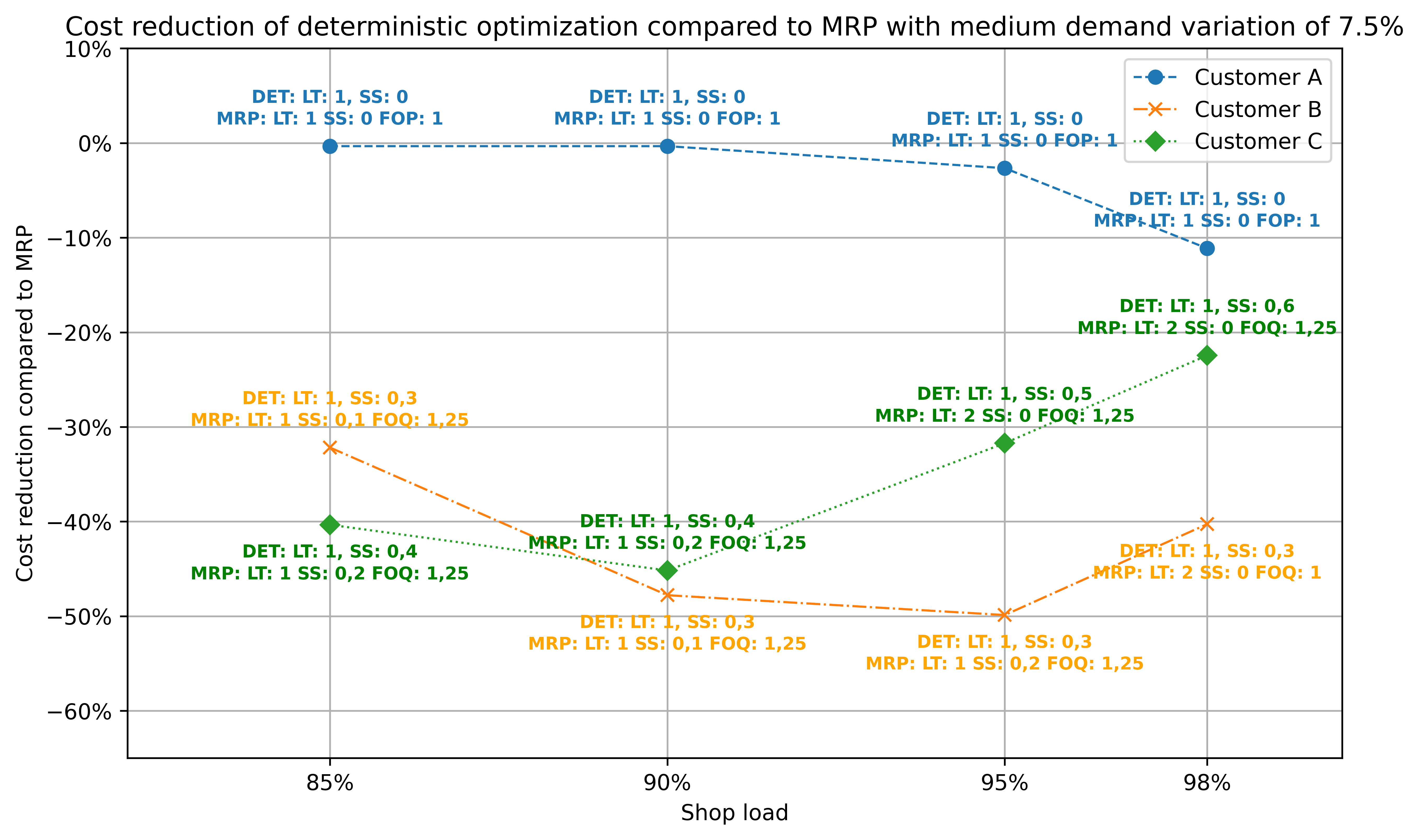
Figure 5: Comparison of deterministic optimization to MRP in a setting with medium demand variation (7.5%) for different shop loads

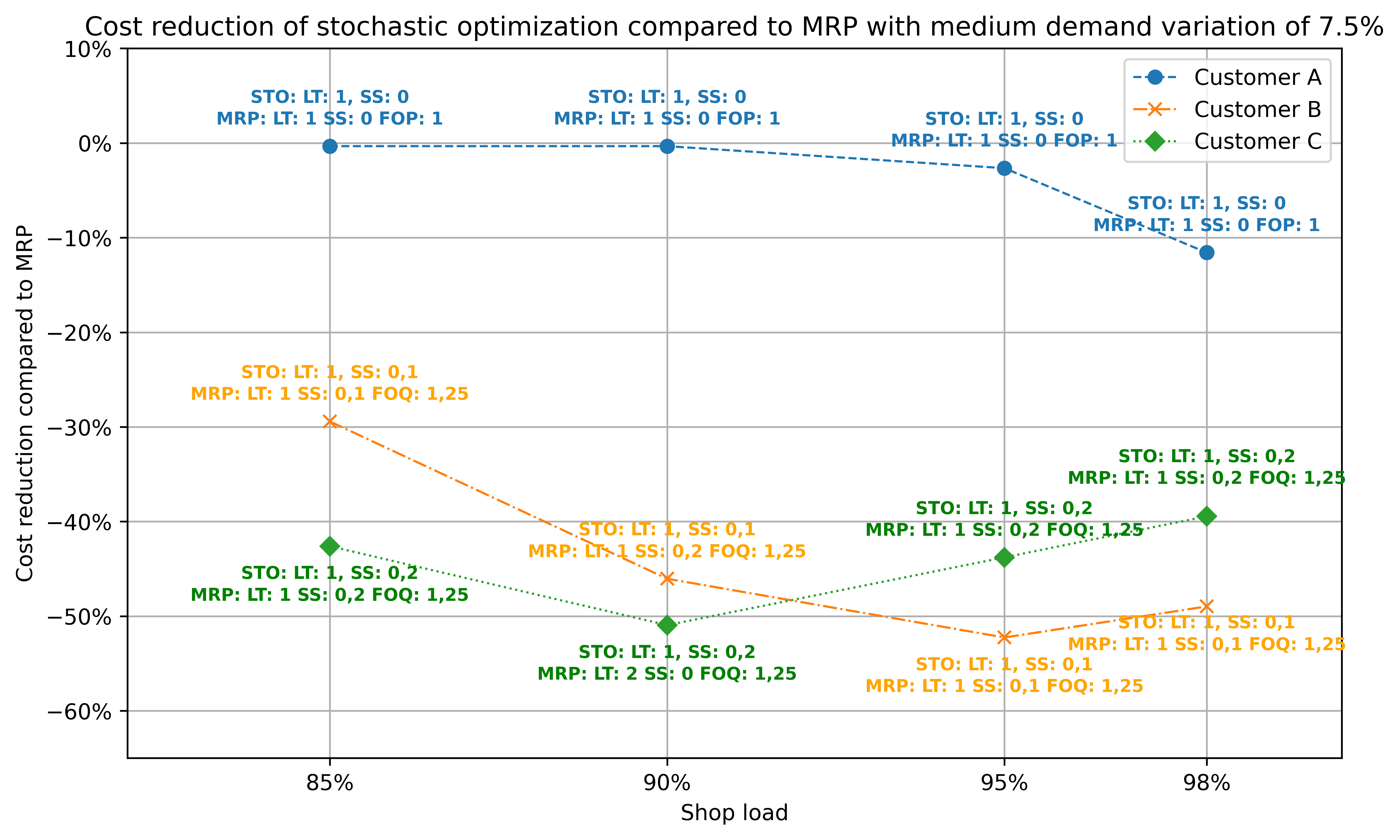
Figure 6: Comparison of stochastic optimization (30 scenarios) to MRP in a setting with medium demand variation (7.5%) for different shop loads

First of all, we note that the demand pattern of Customer A does not include updates, meaning that the stochastic optimization model is equivalent to the deterministic one, since all sampled scenarios represent the same demand. For this reason the performance of deterministic and stochastic optimization is equal for Customer A, i.e. the same cost reduction is reported in Figure 5 and 6. For low resource utilization, the optimization approaches are not able to generate an advantage over standard MRP in the case of customer A. This is reasonable, since customer demand does not necessitate any short-term updates, and the low utilization allows the MRP approach to perfectly fulfill all demands on time. Only when considering high resource utilization, e.g. in the 98% case, we observe limitations of MRP. Standard MRP does not consider resource capacity constraints, which can be problematic in cases of tight capacities. This means that it is unable to recognize short term bottlenecks, which can lead to delayed customer orders, even if the final order quantity is known in advance. Using an optimization model instead allows to consider resource restrictions and to react to upcoming bottleneck situations by partly producing the required amounts in earlier periods. For customers of type A, in the case of medium demand variations and 98%, utilization this planning advantage can reduce the total costs by more than 10% compared to a standard MRP procedure.

Customer B changes demands last minute, meaning that the forecasted quantity does not match the final demand realization. In contrast to Customer A, the production plans obtained by the stochastic model differ from the plans resulting from the deterministic one. First of all, we observe a significant performance improvement of both optimization approaches compared to MRP along all utilizations. For lower utilizations both models, i.e. deterministic and stochastic, lead to similar cost reductions between 30% and 50%. The use of safety stocks allows the deterministic model to hedge against high demand realizations. While the best performing safety stock parameter for the deterministic model is 30% of the average demand, it is only 10% for the stochastic model. The limitations of the deterministic model with safety stocks become visible in the high utilization (98%) setting. While in this case stochastic optimization is able to outperform MRP by almost 50%, the deterministic model results in a lower reduction of 40%.

Finally, Customer C changes demand forecasts every period, which leads to severe instabilities in the production planning. Also for this update pattern both optimization approaches clearly outperform MRP along all utilizations. Again the deterministic models leverage high safety stocks to hedge against demand variations. While a safety stock of 20% of the mean demand leads to the best performance of the stochastic model, the deterministic model uses up to 60% in the high utilization setting. In case of tight resource capacities, the performance improvement of the deterministic approach over MRP reduces to 32% for 95% utilization and 22% for 98% utilization. Applying stochastic optimization on the other hand leads to a cost reduction of more than 40%, even in high utilization environments. This demonstrates the advantage of explicitly considering uncertainty in future demands within the optimization approach.

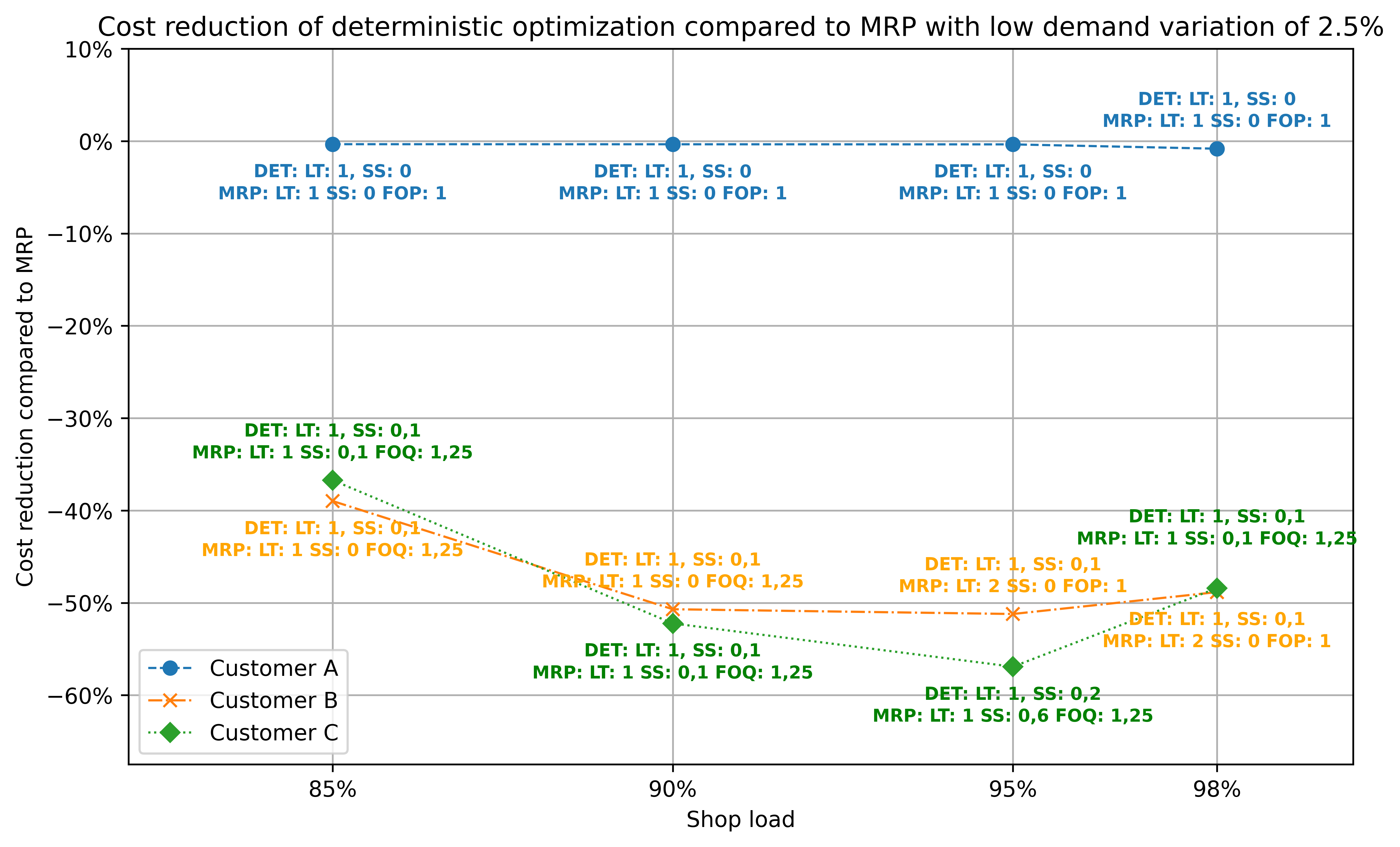
Figure 9: Comparison of deterministic optimization to MRP in a setting with low demand variation (2.5%) for different shop loads

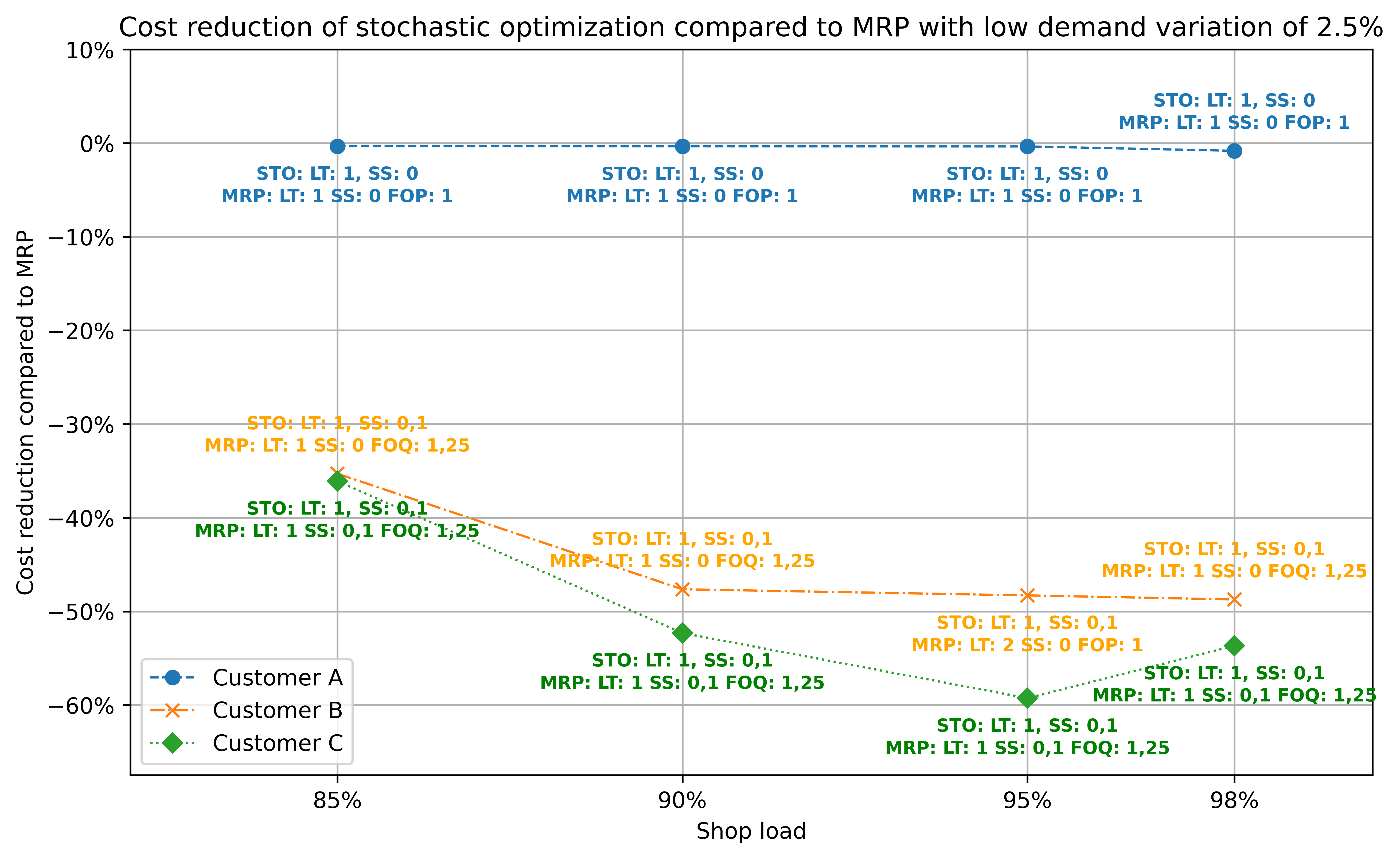
Figure 10: Comparison of stochastic optimization (30 scenarios) to MRP in a setting with low demand variation (2.5%) for different shop loads

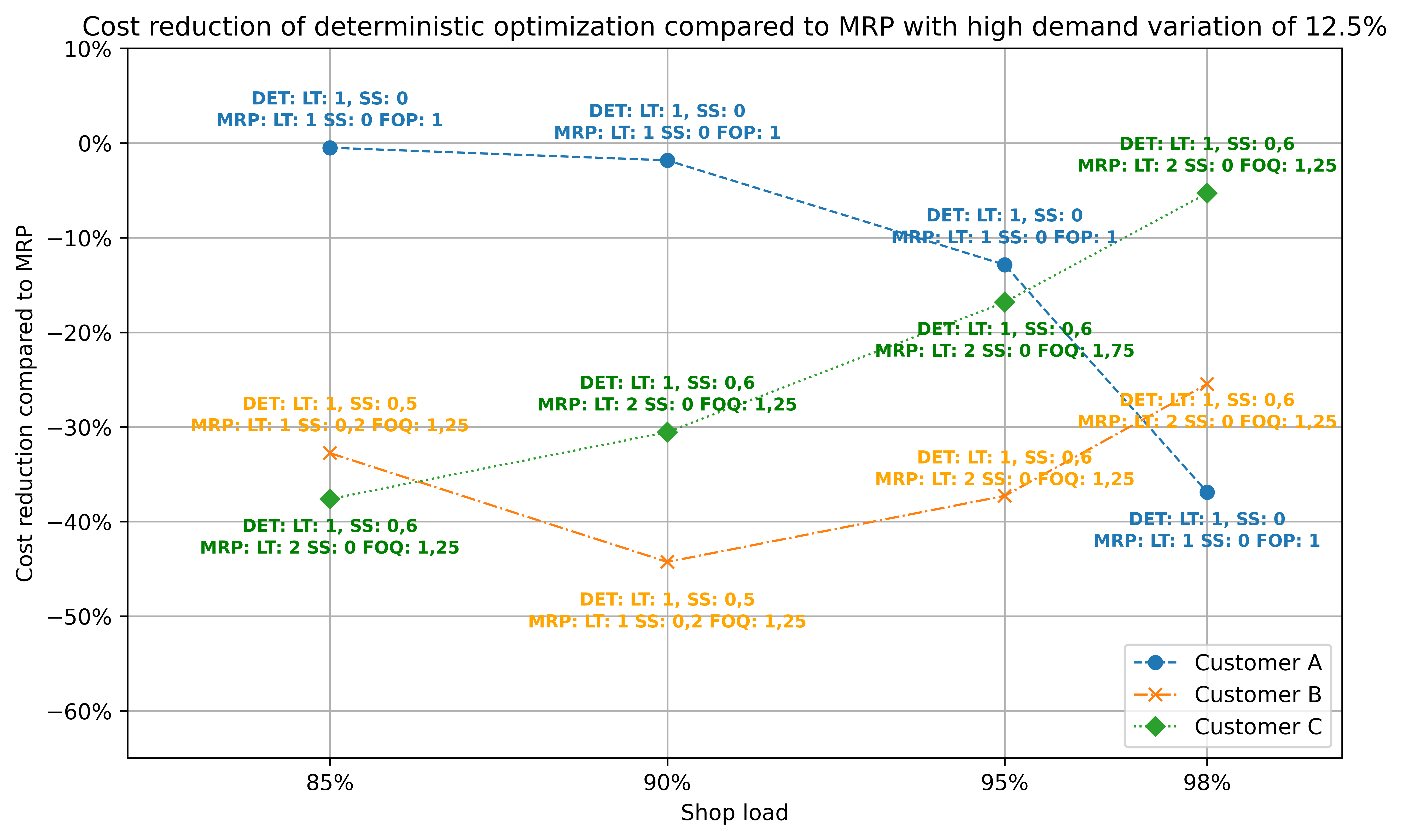
Figure 11: Comparison of deterministic optimization to MRP in a setting with high demand variation (12.5%) for different shop loads

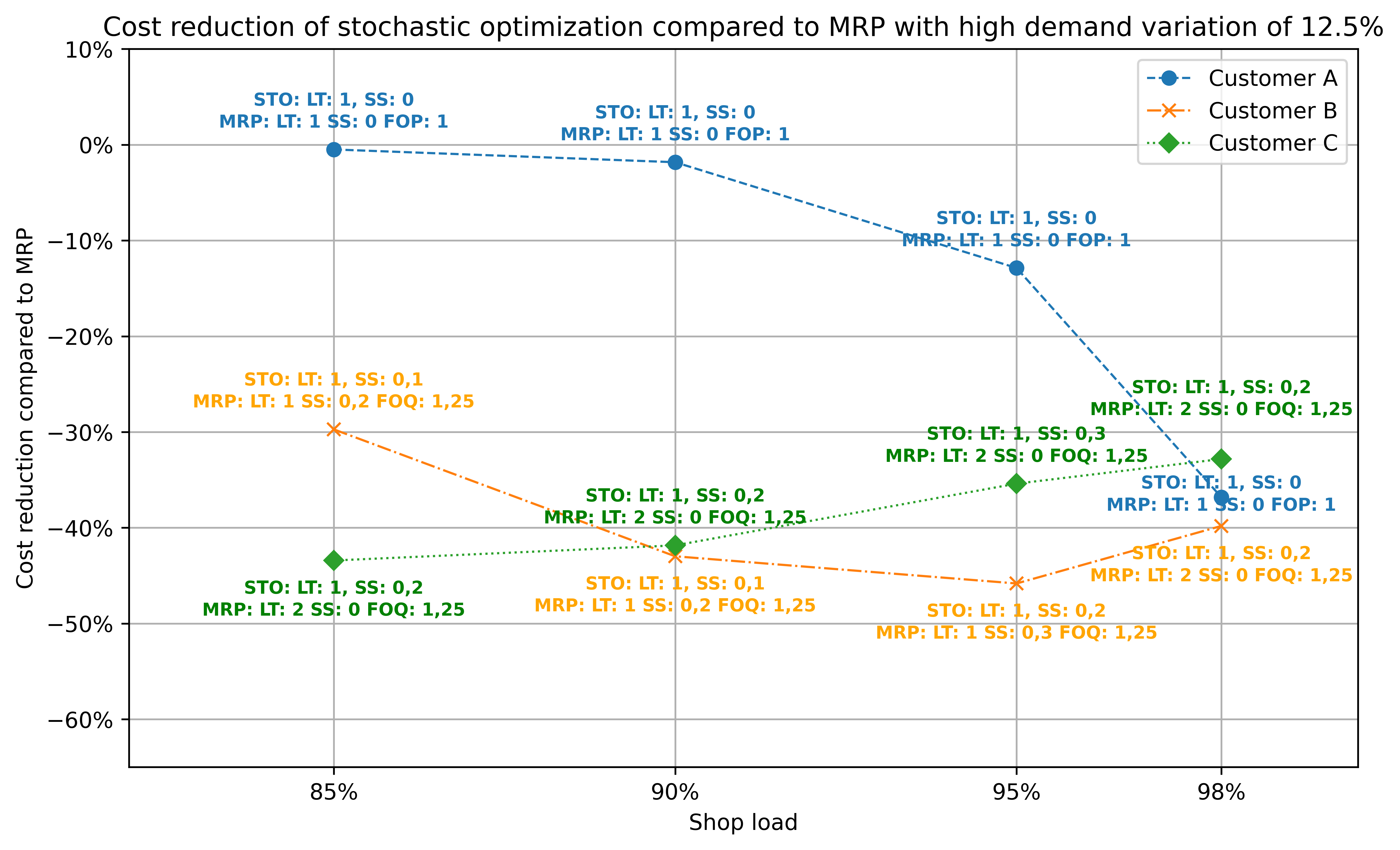
Figure 12: Comparison of stochastic optimization (30 scenarios) to MRP in a setting with high demand variation (12.5%) for different shop loads

In addition to the medium demand variation case (7.5%), we also report results for low demand variation (2.5%) and high demand variation (12.5%) in Figures 9 - 12 in the Appendix. While the discussed differentiation between the optimization approaches is weaker in the low variation case, it is even stronger for high demand variations.

5.4 The impact of forecast uncertainty

In order to assess the impact of increasing uncertainty in demand forecasts, we perform a series of experiments with demand variation values $\alpha$ in the range {2.5%, 5%, 7.5%, 10%, 12.5%}. Figure 7 shows the cost reduction of stochastic optimization over deterministic optimization for a utilization of 95%.

First of all, we observe that for Customer B deterministic optimization outperforms the stochastic model in case of a low demand variation with 2.5%. Planning with the deterministic model and a safety stock of 10% of the mean period demand is enough to balance demand uncertainties and leads to a 6% cost reduction over the stochastic approach. With increasing demand variation we, however, see the advantage of using stochastic optimization. The deterministic model leverages increasing safety stocks to hedge against the growing variability in the demands, using 30% for a demand variation of 7.5% and up to 60% for high variation of 12.5%. This increased safety stock weakens the performance of the deterministic approach and allows the stochastic model, which keeps the safety stock at a moderate level of 10%-20%, to result in reduced overall costs. While the performance improvement is 5% for medium demand variation of 7.5%, it is 14% in case of high variation with 12.5%.

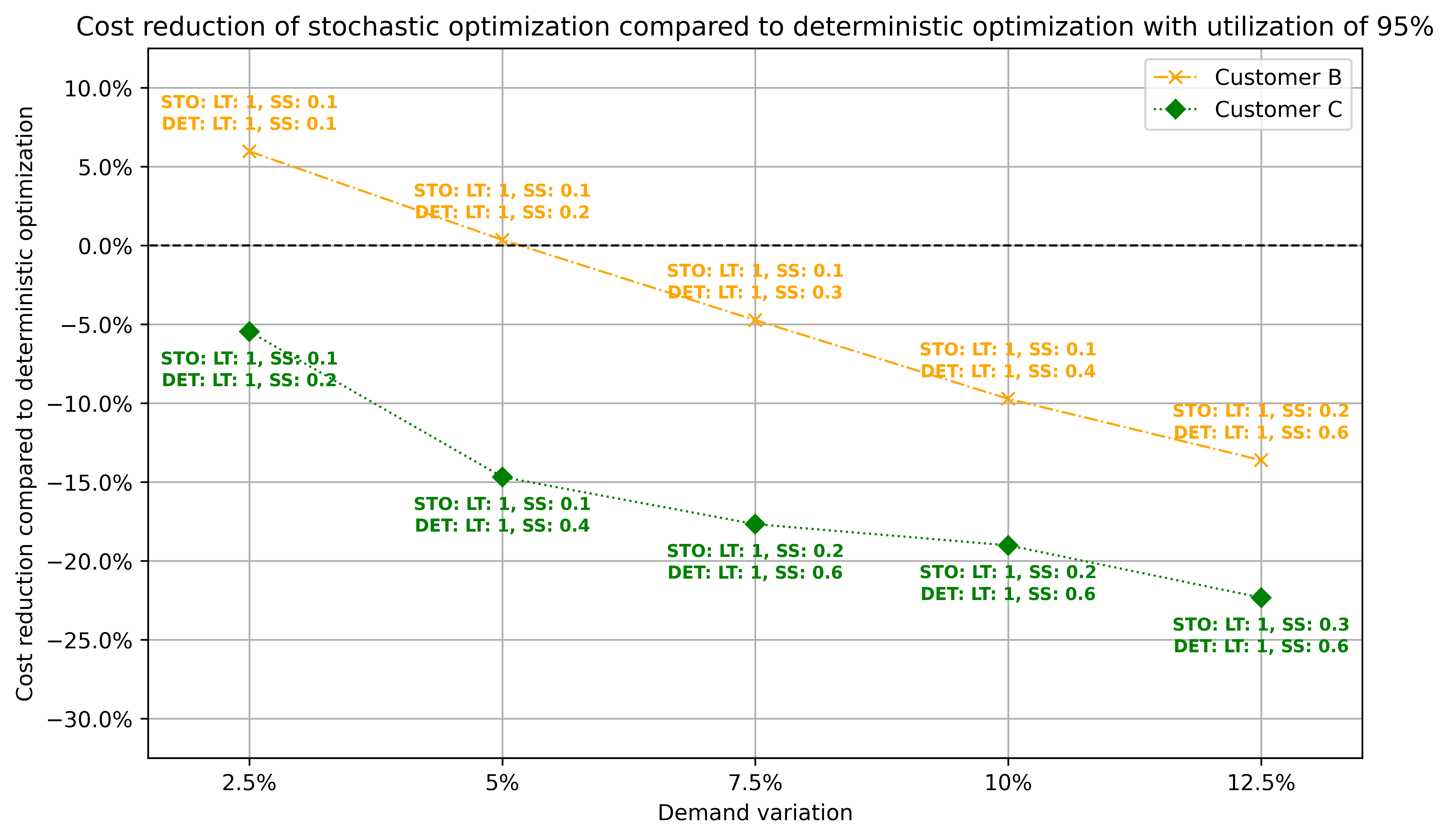
Figure 7: Comparison of stochastic optimization (30 scenarios) to deterministic optimization with a utilization of 95% for different demand variations

Deterministic optimization could not outperform the stochastic approach for Customer C in the 95% utilization setting. Even for low demand variation of 2.5%, solving the stochastic model reduced the resulting overall costs by 5% compared to the deterministic version. This improvement further increased with higher demand variation leading to a 23% reduction in costs for high demand variation with 12.5%. Again we see that the deterministic model increases safety stocks to cope with high variability in the customer demands, storing up to 60% of the average demands as a buffer. For the stochastic approach on the other hand a lower safety stock of 30% is sufficient, due to its capability to anticipate possible variations in the upcoming periods.

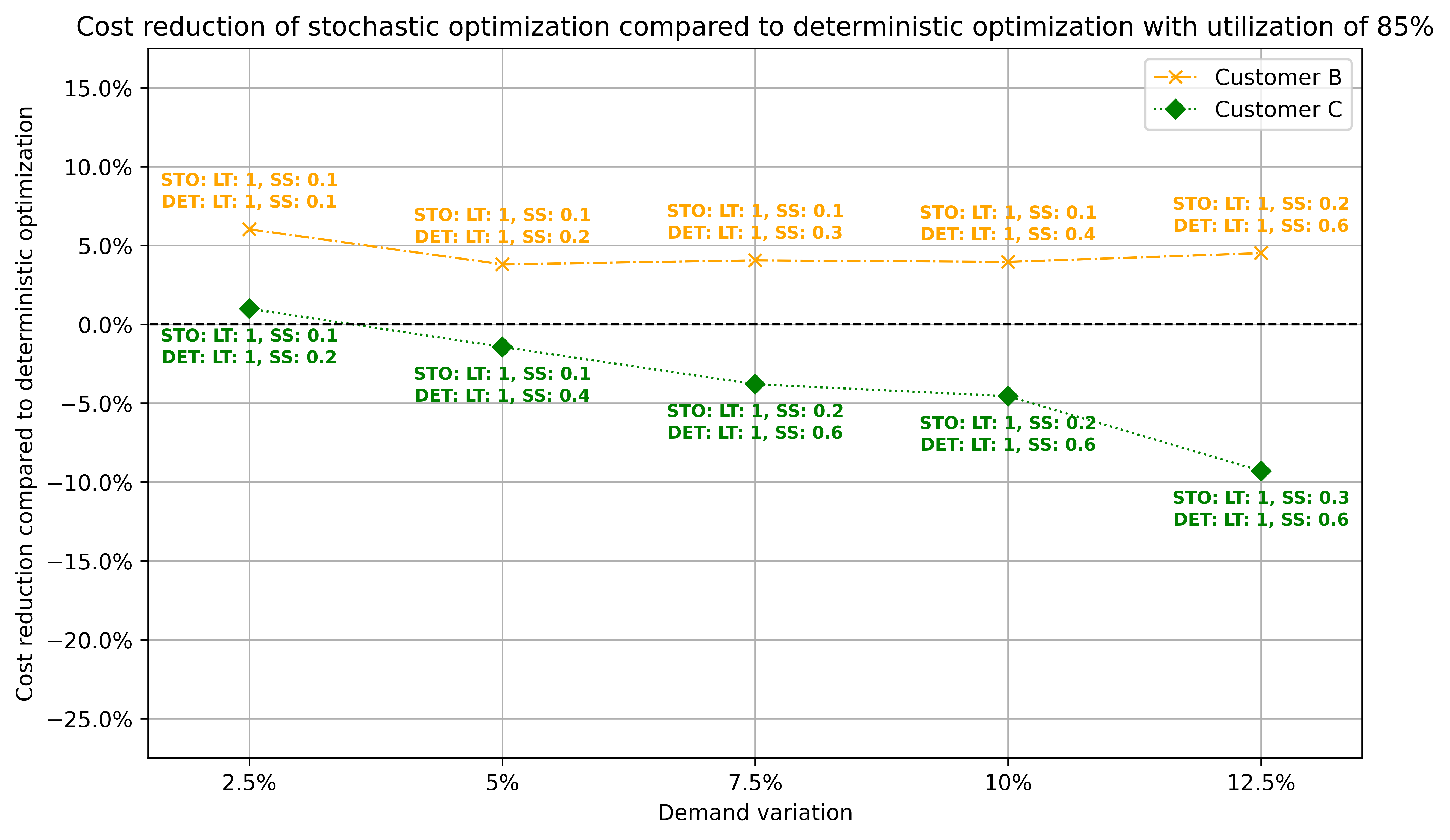
Figure 13: Comparison of stochastic optimization (30 scenarios) to deterministic optimization with a utilization of 85% for different demand variations

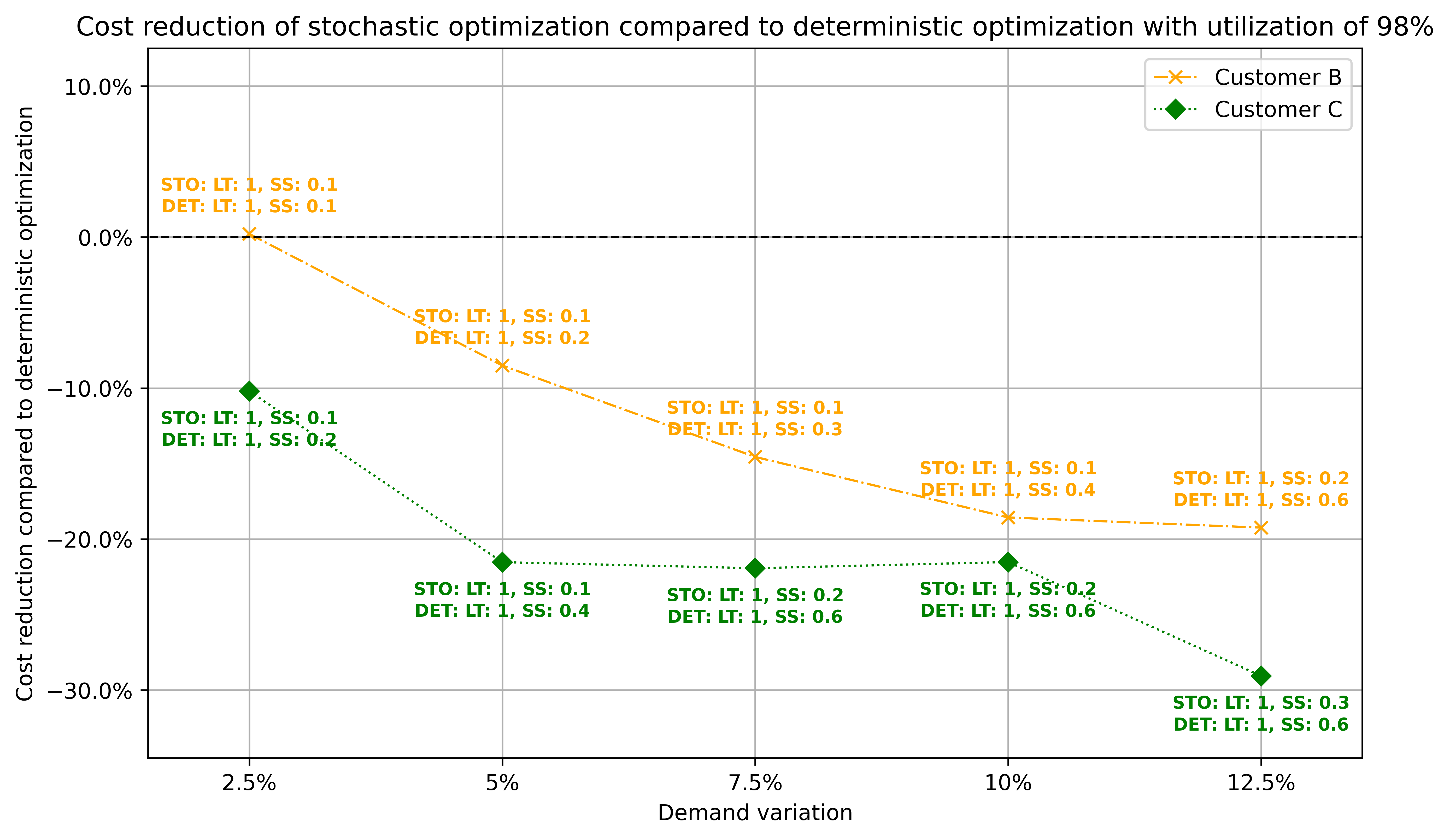
Figure 14: Comparison of stochastic optimization (30 scenarios) to deterministic optimization with a utilization of 98% for different demand variations

Additionally, in Figure 13 and Figure 14 we report the results for the low utilization of 85% and high utilization of 98% case in the Appendix. The low utilization case demonstrates that deterministic optimization with safety stocks is sufficient for Customer B if enough resource capacity is available. It outperforms the stochastic approach for all demand variations. For Customer C solving the stochastic model is advantageous and cost improvements of up to 10% over the deterministic version are possible. In high utilization environments of 98%, stochastic optimization outperforms the deterministic model for both customer types B and C and over all demand variations. While improvements of up to 20% are possible for Customer B, a cost reduction of up to 30% can be reached for Customer C.

5.5 General overview

In this section, we summarize the results presented so far. Table 4 provides an overview of the respective performance of the three approaches across different utilizations, customer demand update patterns and demand variations. We display the cost values and best performing parameter sets, out of the evaluated settings. Moreover for each planning situation, meaning a combination of customer type, demand variation and utilization, we report the relative cost difference ($\%\Delta$) of the best planning approach in percentage compared to standard MRP. The best performing model for each planning situation is highlighted in bold.

		Utilization 85%							Utilization 90%
Customer	Variation	MRP		Deterministic		Stochastic		%$\Delta$	MRP		Deterministic		Stochastic		%$\Delta$
		(LT,SS,LSP)		(LT,SS)		(LT,SS)			(LT,SS,LSP)		(LT,SS)		(LT,SS)
A1	2.5%	1209	(1,0,P: 1)	1205	(1,0)	-		0%	1174	(1,0,P: 1)	1170	(1,0)	-		0%
A1	5.0%	1209	(1,0,P: 1)	1205	(1,0)	-		0%	1173	(1,0,P: 1)	1169	(1,0)	-		0%
A1	7.5%	1208	(1,0,P: 1)	1204	(1,0)	-		0%	1173	(1,0,P: 1)	1169	(1,0)	-		0%
A1	10.0%	1207	(1,0,P: 1)	1203	(1,0)	-		0%	1178	(1,0,P: 1)	1169	(1,0)	-		-1%
A1	12.5%	1208	(1,0,P: 1)	1202	(1,0)	-		0%	1195	(1,0,P: 1)	1173	(1,0)	-		-2%
B2	2.5%	2179	(1,0,Q: 1.25)	1330	(1,0.1)	1410	(1,0.1)	-39%	2626	(2,0,P: 1)	1295	(1,0.1)	1375	(1,0.1)	-51%
B2	5.0%	2212	(1,0.1,Q: 1.25)	1450	(1,0.2)	1505	(1,0.1)	-34%	2901	(1,0.1,Q: 1.25)	1419	(1,0.2)	1469	(1,0.1)	-51%
B2	7.5%	2306	(1,0.1,Q: 1.25)	1564	(1,0.3)	1628	(1,0.1)	-32%	2952	(1,0.2,Q: 1.25)	1542	(1,0.3)	1593	(1,0.1)	-48%
B2	10.0%	2455	(1,0.2,Q: 1.25)	1680	(1,0.4)	1746	(1,0.1)	-32%	3063	(1,0.2,Q: 1.25)	1675	(1,0.4)	1722	(1,0.1)	-45%
B2	12.5%	2675	(1,0.2,Q: 1.25)	1798	(1,0.5)	1880	(1,0.1)	-33%	3263	(1,0.3,Q: 1.25)	1818	(1,0.5)	1860	(1,0.2)	-44%
C3	2.5%	2202	(1,0.1,Q: 1.25)	1394	(1,0.1)	1408	(1,0.1)	-37%	2877	(1,0.1,Q: 1.25)	1375	(1,0.1)	1372	(1,0.1)	-52%
C3	5.0%	2423	(1,0.1,Q: 1.25)	1560	(1,0.3)	1538	(1,0.1)	-37%	3174	(1,0.2,Q: 1.25)	1603	(1,0.3)	1525	(1,0.1)	-52%
C3	7.5%	2983	(1,0.2,Q: 1.25)	1780	(1,0.4)	1712	(1,0.2)	-43%	3583	(2,0,Q: 1.25)	1964	(1,0.5)	1757	(1,0.2)	-51%
C3	10.0%	3613	(1,0.3,Q: 1.25)	1970	(1,0.5)	1880	(1,0.2)	-48%	3628	(2,0,Q: 1.25)	2284	(1,0.5)	1969	(1,0.2)	-46%
C3	12.5%	3619	(2,0,Q: 1.25)	2258	(1,0.6)	2048	(1,0.2)	-43%	3738	(2,0,Q: 1.25)	2596	(1,0.6)	2174	(1,0.3)	-42%
Average		2181		1520		1518			2513		1561		1511
		Utilization 95%							Utilization 98%
Customer	Variation	MRP		Deterministic		Stochastic		%$\Delta$	MRP		Deterministic		Stochastic		%$\Delta$
		(LT,SS,LSP)		(LT,SS)		(LT,SS)			(LT,SS,LSP)		(LT,SS)		(LT,SS)
A1	2.5%	1138	(1,0,P: 1)	1134	(1,0)	-		0%	1126	(1,0,P: 1)	1117	(1,0)	-		-1%
A1	5.0%	1142	(1,0,P: 1)	1135	(1,0)	-		-1%	1220	(1,0,P: 1)	1145	(1,0)	-		-6%
A1	7.5%	1175	(1,0,P: 1)	1143	(1,0)	-		-3%	1443	(1,0,P: 1)	1282	(1,0)	-		-11%
A1	10.0%	1246	(1,0,P: 1)	1157	(1,0)	-		-7%	1837	(1,0,P: 1)	1416	(1,0)	-		-23%
A1	12.5%	1362	(1,0,P: 1)	1187	(1,0)	-		-13%	2411	(1,0,P: 1)	1521	(1,0)	-		-37%
B2	2.5%	2591	(2,0,P: 1)	1264	(1,0.1)	1339	(1,0.1)	-51%	2578	(2,0,P: 1)	1319	(1,0.1)	1322	(1,0.1)	-49%
B2	5.0%	3313	(2,0,Q: 1)	1427	(1,0.2)	1432	(1,0.1)	-57%	3252	(2,0,Q: 1)	1657	(1,0.3)	1516	(1,0.1)	-53%
B2	7.5%	3274	(2,0,Q: 1)	1641	(1,0.3)	1563	(1,0.1)	-52%	3451	(2,0,Q: 1.25)	2061	(1,0.4)	1761	(1,0.1)	-49%
B2	10.0%	3464	(1,0.6,Q: 1.25)	1906	(1,0.4)	1721	(1,0.1)	-50%	3457	(2,0,Q: 1.25)	2352	(1,0.5)	1916	(1,0.2)	-45%
B2	12.5%	3537	(2,0,Q: 1.25)	2218	(1,0.6)	1916	(1,0.2)	-46%	3501	(2,0,Q: 1.25)	2609	(1,0.6)	2107	(1,0.2)	-40%
C3	2.5%	3306	(1,0.6,Q: 1.25)	1424	(1,0.2)	1347	(1,0.1)	-59%	3370	(2,0.1,P: 2)	1739	(1,0.3)	1562	(1,0.1)	-54%
C3	5.0%	3482	(2,0,Q: 1.25)	1974	(1,0.4)	1684	(1,0.1)	-52%	3415	(2,0,Q: 1.25)	2387	(1,0.6)	1873	(1,0.2)	-45%
C3	7.5%	3544	(2,0,Q: 1.25)	2419	(1,0.6)	1992	(1,0.2)	-44%	3620	(2,0,Q: 1.5)	2807	(1,0.6)	2192	(1,0.2)	-39%
C3	10.0%	3736	(2,0,Q: 1.5)	2842	(1,0.6)	2302	(1,0.2)	-38%	3969	(2,0,Q: 1.75)	3320	(1,0.6)	2606	(1,0.2)	-34%
C3	12.5%	3988	(2,0,Q: 1.75)	3317	(1,0.6)	2577	(1,0.3)	-35%	4352	(2,0.1,Q: 2)	4122	(2,0.5)	2924	(1,0.4)	-33%
Average		2687		1746		1575			2867		2057		1750
1no changes, 2change at due date, 3change every period
LSP = lot size policy, LT = lead time, P = fixed order period, Q = fixed order quantity, SS = safety stock, %$\Delta$ = cost reduction to MRP

Table 4: General cost and parameter overview across different resource utilizations, customer demand update patterns and demand variations. Comparison of MRP (LT,SS,LSP), deterministic optimization (LT,SS) and stochastic optimization (LT,SS) (for 30 scenarios)

For each planning approach we observe an increase in average overall costs with higher utilization. This is reasonable, since tight resource capacities restrict the opportunities of the planning methods and lead to costly delays. We summarize that the use of optimization models does not yield an advantage over standard MRP for reliable customers (type A) that do not change their demands in the short term, as long as resource utilization is moderately low (85% and 90%). We again highlight that the stochastic model is equivalent to the deterministic version for Customer A and we therefore only report the results of the deterministic model. In case of higher utilizations (95% and 98%) applying MRP is problematic even for the reliable Customer A if demand variation is high, leading to an irregular demand pattern that causes short term bottlenecks in the production system. The use of optimization approaches that consider the available resource capacities can counteract these bottlenecks and reduce the resulting costs by up to 13% in the 95% utilization case and up to 37% in the 98% utilization case.

Customer B updates demands once in the short term. This leads to delays if the amount of produced items is not sufficient to satisfy the realized demand and causes higher inventories in case of low demand realizations. We summarize that for Customer B the use of deterministic models using safety stocks is most efficient in case of low resource utilization (85% and 90%) across all demand variations. The availability of buffer capacity allows the method to counteract increasing demand variation by producing higher safety stocks. Significant cost reductions of up to 50% over standard MRP are possible. When considering higher utilization environments (95% and 98%) we observe a shift towards the stochastic optimization model. Tight capacity limitations are problematic for the creation of large safety stocks and cause a decline in the deterministic performance. Especially for large demand variations, planning by means of the stochastic optimization model outperforms the deterministic approach.

Finally, Customer C updates demands frequently representing the highest level of demand uncertainty. For this customer type we see a superior performance of the stochastic planning approach across all utilizations and demand variations. Despite relying on large safety stocks, the deterministic model is not able to provide production plans that are suited for the uncertain environment. Customer C highlights the ability of the stochastic optimization model to explicitly incorporate information on uncertain future demand realizations during the planning procedure. Leveraging stochastic optimization in highly uncertain demand settings, as they are modelled by customer type C, can lead to cost reductions of over 50% compared to standard MRP.

6 Conclusion

In this work we combine a stochastic optimization model for multi-item multi-echelon capacitated lot sizing with discrete-event simulation in order to generate a rolling horizon production planning framework. Making use of stochastic optimization allows to explicitly consider customer demand fluctuations in the lot sizing process. We compare the stochastic planning approach to a deterministic optimization model using mean demands, as well as to a standard MRP approach. We evaluate the different planning methods by means of the developed discrete-event simulation environment and report the resulting overall costs.

From a managerial perspective we conclude that the standard MRP approach is sufficient in case of production environments with low resource utilization and customer demands that underlie almost no uncertainty, meaning that the realized demands correspond to the forecasted values. In case of tight resource restrictions, the MRP approach is unable to anticipate capacity bottlenecks, caused by irregular demand patterns, even though demands do not change in the short term. For this scenario the use of optimization approaches helps to smooth the utilization of resources and counteracts the occurrence of bottlenecks.

In situations where customers change their forecasted demands last minute, standard MRP is not competitive with the use of optimization models. While solving a deterministic model using safety stocks works well for scenarios with low utilization, its effectiveness diminishes in situations with tight resource capacities. In contrast, using stochastic optimization takes into account demand uncertainty, creating a bridge to more effective production plans that remain robust even under high levels of utilization. This is especially true if customers frequently update their demand forecasts implying a high level of uncertainty for future demands.

For future work, we plan to replace the two-stage stochastic optimization approach with a more advanced multi-stage model that explicitly takes the possibility for adjustments in later periods into account. Moreover, we plan to evaluate more complex production systems by investigating the impact of the number of different items and production levels.

Funding

This research was funded in whole, or in part, by the Austrian Science Fund (FWF) [P 32954-G]. For the purpose of open access, the author has applied a CC BY public copyright licence to any Author Accepted Manuscript version arising from this submission.

Data availability statement

The data that support the findings of this study are available in Zenodo at 10.5281/zenodo.10686729 upon reasonable request to Wolfgang Seiringer.

Appendix A Additional figures