Abstract

Time-series with time-varying variance pose a unique challenge to uncertainty quantification (UQ) methods. Time-varying variance, such as volatility clustering as seen in financial time-series, can lead to large mismatch between predicted uncertainty and forecast error. Building on recent advances in neural network UQ literature, we extend and simplify Deep Evidential Regression and Deep Ensembles into a unified framework to deal with UQ under the presence of volatility clustering. We show that a Scale Mixture Distribution is a simpler alternative to the Normal-Inverse-Gamma prior that provides favorable complexity-accuracy trade-off. To illustrate the performance of our proposed approach, we apply it to two sets of financial time-series exhibiting volatility clustering: cryptocurrencies and U.S. equities.

Keywords— neural network; uncertainty quantification; time-series; volatility clustering

1 Introduction

Asset returns are known to exhibit irregular bursts of high volatility that cluster in time (termed volatility clustering; Cont,, 2001). This poses a challenge to practitioners during portfolio construction which involves the trade-off of return and risk. To motivate the discussion, consider the following simple thought experiment. Suppose an investor has a model that can perfectly forecast next day’s asset returns and that the investor’s goal is to maximize terminal wealth. Then, on each day, the most rational decision would be to place all of the investor’s wealth into the asset with the highest expected return on the next day. Next, suppose that the investor’s model is a noisy estimator of future asset returns. Then, the investor may choose to diversify across multiple assets. This has led to the development of various models for optimal bet allocation that depend on some measures of risk, such as Kelly criterion (Kelly,, 1956; Byrnes and Barnett,, 2018) and Bayesian-based portfolio optimization (Black and Litterman,, 1991).

Forecast uncertainty has an important role in many applications. Such quantity is easy to obtain for statistical models such as linear regression. However, classical neural networks for regression problems are typically trained using MSE and provide point estimates for the mean prediction conditional on the input without regards for the conditional variance (see Goodfellow et al.,, 2016). As a modeller (in our case, an investor), one is concerned with predictive uncertainty (Gawlikowski et al.,, 2021). This is the total uncertainty around a point estimate. Predictive uncertainty can be decomposed into (Gruber et al.,, 2023): aleatoric uncertainty, and epistemic uncertainty. Aleatoric uncertainty originates from the stochastic relationship between input variable $X$ taking value $x$ and output variable $Y$ (Gruber et al.,, 2023). As long as the conditional distribution of $Y|x$ is not degenerate (i.e., $Y$ cannot be perfectly predicted), there will always be aleatoric uncertainty. Aleatoric uncertainty does not typically depend on sample size. By contrast, epistemic uncertainty is attributable to the model and typically scales inversely with sample size (Meinert et al.,, 2022). Epistemic uncertainty can be further decomposed into model uncertainty, which relates to the correct specification of the model, and parametric uncertainty, which relates to the correct estimation of model parameters (Sullivan,, 2015; Gruber et al.,, 2023). Epistemic uncertainty refers to the part of predictive uncertainty that is reducible through additional information (e.g., more observations and additional variables). In practice, a clear separation between aleatoric and epistemic uncertainties is often impossible. To illustrate, consider the (fair) dice rolling experiment, commonly considered to be a process of pure randomness. However, if the initial position and each rotation of the dice can be measured, then it is possible to predict the outcome of each dice roll (Hora,, 1996; Gruber et al.,, 2023). Thus, what is truly aleatoric (i.e., unpredictability of dice roll) and what is epistemic (i.e., initial position and rotation of the dice are merely missing variables) may be difficult to disentangle from a philosophical perspective.

Traditionally, neural network uncertainty quantification (UQ) requires the use of Bayesian methods or evaluation of the model in unseen data (Meinert et al.,, 2022). A Bayesian neural network (BNN) is a full probabilistic interpretation of neural network, by placing priors on network weights and inducing a distribution over a parametric set of functions (MacKay,, 1992; Neal,, 1996; Gal,, 2016). Modern BNNs can be trained using Markov Chain Monte Carlo (MCMC, e.g., the Metropolis-Hastings algorithm; Hastings,, 1970) and Variational Inference techniques (Jospin et al.,, 2022). Jospin et al., (2022) notes four advantages of using BNNs over classical neural networks, with two being relevant to UQ. First, Bayesian methods provide a natural approach to UQ and are better calibrated than classical neural networks (Mitros and Namee,, 2019; Kristiadi et al.,, 2020; Ovadia et al.,, 2019; Jospin et al.,, 2022). Second, BNN allows distinguishing between epistemic uncertainty and aleatoric uncertainty. However, despite their advantages, MCMC-based methods are computationally expensive (Quiroz et al.,, 2019). Thus, limiting the applicability of BNNs.

Recent advances (see Gawlikowski et al.,, 2021 for a recent survey) have focused on predicting the conditional distribution that is most likely to have generated the data and thus bridging the gap between BNNs and classical neural networks. In particular, using a neural network to generate parameters of a conditional distribution that is assumed to have generated the data (Lakshminarayanan et al.,, 2017; Amini et al.,, 2020) offers an attractive trade-off between adequately quantifying uncertainty and avoiding the computational cost of a full Bayesian treatment. In Lakshminarayanan et al., (2017) (the Ensemble method, also know as Deep Ensembles), regression target $y$ is assumed to be drawn from $y\sim\operatorname{N}(\mu,\sigma^{2})$, where $\operatorname{N}$ is the Normal distribution, $\mu$ is the expectation of $y$ and $\sigma^{2}$ models aleatoric uncertainty. In this setup, $\sigma^{2}$ is incapable of quantifying epistemic uncertainty. Lakshminarayanan et al., (2017) addressed this by using an ensemble of neural networks with randomly initialized weights. Each network settles in a different local minima and produces different $\mu$ and $\sigma^{2}$ for the same input. The variance of $\mu$ across the ensemble thus provides an estimate of epistemic uncertainty. Addressing this shortcoming, Amini et al., (2020) (the Evidential method, also know as Deep Evidential Regression) proposed to place an evidential prior, the Normal-Inverse-Gamma distribution (NIG), on $\mu,\sigma^{2}$. In this construct, prediction $\mu$ is assumed to be drawn from the priors: $\mu\sim\operatorname{N}(\gamma,\sigma^{2}\nu^{-1})$ and $\sigma^{2}\sim\operatorname{InvGam}(\alpha,\beta)$, where $\sigma^{2}$ remains as an estimate of aleatoric uncertainty, $\operatorname{InvGam}$ (or $\operatorname{IG}$) is the Inverse-Gamma distribution and $\sigma^{2}\nu^{-1}$ (with $\sigma^{2}\sim\operatorname{InvGam}(\alpha,\beta)$) is estimated epistemic uncertainty. Epistemic uncertainty is linked to aleatoric uncertainty via $\nu$, which is learnt from the data. The marginal distribution of a Normal likelihood with NIG prior is the Student’s t-distribution. This mimics a Bayesian setup and circumvents the costly computational burden of MCMC methods by analytically integrating out unobserved variables. Ensemble and Evidential require only minimal modifications to a conventional neural network architecture — requiring only the negative log-likelhood (NLL) function of the marginal distribution as loss function and a new output layer. Evidential has been applied to navigation (Liu et al.,, 2021; Cai et al.,, 2021; Singh et al.,, 2022) and medical fields (Soleimany et al.,, 2021; Li and Liu,, 2022), and has been extended into the multi-task learning domain (Oh and Shin,, 2022). Multivariate models related to Evidential include the Natural Posterior Network which also uses a conjugate prior (NIG for regression problems and Dirichlet for categorical classification problems; Charpentier et al.,, 2021), and Regression Prior Networks which uses a Normal-Wishart prior (Malinin et al.,, 2020).

However, more recent works have highlighted weaknesses of the Evidential method. Scoring rules are a class of loss functions that measure the discrepancy between a predicted distribution and the observed distribution (Gneiting and Raftery,, 2007). A scoring rule is proper if the score is maximized when the discrepancy is minimized, and is strictly proper if the maximum is unique. Thus, strictly proper scoring rules provide attractive loss functions for scoring probabilistic forecasts. Evidential can be interpreted as a hierarchical method with a prior distribution that controls the data distribution. Bengs et al., (2023) argues that in order for hierarchical methods such as Evidential to comply with the requirements of proper scoring rules, rather than training on observable values of $y$, the predictor must be trained on the imaginary distribution around each observation that depicts its uncertainty, which cannot possibly exist. This requirement stems from the definition of proper scoring, which requires the learner be scored against the “ground truth”. As $\alpha$ and $\beta$ relate to the prior distribution in Evidential, they are not directly observed as data. Thus, hierarchical methods lack theoretical guarantee on the robustness of their estimated distributions. Similarly, Meinert et al., (2022) argued that unlike aleatoric uncertainty, epistemic uncertainty has no “ground truth” and is difficult to estimate objectively. To motivate this argument, Meinert et al., (2022) used the example of points lined up perfectly in a straight line. If one point is perturbed such that the points no longer form a straight line. Without relying on a-priori assumptions, it is impossible to perform point-wise separation of aleatoric and epistemic uncertainties (i.e., whether the single deviation is due to noise or correctness of the linear model and its estimated slope). The marginal t-distribution of NIG is overparameterized, which leads to the finding that it is possible to minimize the NLL irrespective of $\nu$ (interpreted as “strength of the data” in Amini et al.,, 2020). As a further critique of the network architecture, we note that all four hyperparameters of Evidential are derived from the same latent representation outputted by the last hidden layer. The four hyperparameters can have vastly different scales (e.g., in our motivating application, $\gamma$ is in scale of 0.01, while $\nu$ is in scale of 10). We consider this feature to be a weakness of these approaches as the latent representation has to provide a sufficiently rich encoding to linearly derive all hyperparameters of the distribution. Nonetheless, successful applications of Evidential on real world datasets has led Meinert et al., (2022) to conclude that Evidential is a heuristic to Bayesian methods and may be appropriate for applications that aim to capture both aleatoric and epistemic uncertainties but do not demand an accurate distinction between them, such as our motivating application.

In this work, we are concerned with neural network UQ for time-series that exhibit time-varying variance, such as time-series of asset returns. We combine and extend Ensemble and Evidential into a framework (the Combined method) for quantifying forecast uncertainty of this class of time-series. We propose to formulate the problem using the scale mixture distribution (SMD), a simpler alternative to the NIG prior, to address some of the shortcomings highlighted by Meinert et al., (2022) and Bengs et al., (2023). In SMD, a sole Gamma prior is placed on the scaling factor of variance of the Normal distribution, rather than both the mean and variance in Evidential. This is motivated by our asset return forecasting application, where the mean is typically close to zero (in scale of 0.01) and thus uncertainty is negligible, and volatility is significantly larger (standard deviation in scale of 0.1). This is consistent with fitting a return series with models such as Generalized ARCH (GARCH; Bollerslev,, 1986) in which the mean process is typically assumed zero or first order autoregressive (Carroll and Kearney,, 2009). Integrating out the scaling factor of SMD results in a marginal t-distribution, of which its variance indicates the predictive uncertainty. Epistemic uncertainty is assumed to be the difference between variance of the marginal t-distribution and variance of the assumed Normal data distribution. This simplification trades off granular attribution of aleatoric and epistemic uncertainties afforded by the NIG prior but allows the reduction of the number of effective parameters by one and resolves the overparameterization of NIG, as highlighted by Meinert et al., (2022). We also propose a novel architecture to model parameters of the marginal distribution using disjoint subnetworks, rather than a single output layer as in Ensemble and Evidential. We show through an ablation study in Section 4.2 that this is crucial to forecasting predictive uncertainty that closely tracks forecast error when the time-series exhibit volatility clustering. As both forecast accuracy and estimation of predictive uncertainty are important to our motivating application, we incorporate model averaging into our Combined method and show that it significantly improves forecast accuracy without significantly changing the estimated predictive uncertainty. This work also provides a template for UQ in time-series that exhibit volatility clustering, such as time-series of asset returns.

To illustrate our contributions, we apply our proposed method to cryptocurrency and U.S. equities time-series forecasting. Cryptocurrencies are an emerging class of digital assets. They are highly volatile and frequently exhibit price bubbles (Fry and Cheah,, 2016; Hafner,, 2018; Chen and Hafner,, 2019; Núñez et al.,, 2019; Petukhina et al.,, 2021), with large volumes of high frequency data (e.g., prices in hourly intervals) freely available from major exchanges. This makes cryptocurrencies an ideal testbed for UQ methodologies in financial applications. Given the extreme levels of volatility, we view cryptocurrencies as one of the most challenging datasets for this type of application. A comparison in U.S. equities is also provided which illustrates performance in conventional financial time-series. In the rest of this paper, we first describe the setup of our motivating application (asset return forecasting) in Section 2.1 and review of related works in Section 2.2. We describe our proposed framework in Section 3. Data description and empirical results of applying Ensemble, Evidential and Combined on cryptocurrency and U.S. equities are detailed in Section 4. Whilst this paper is focused on UQ in time-series that exhibit volatility clustering, in Appendix A.1, we also provide a direct comparison to Evidential and Ensemble using the University of California Irvine Machine Learning Repository (UCI) benchmark datasets (non-time-series), as previously analysed in Hernández-Lobato and Adams, (2015), Gal and Ghahramani, (2016), Lakshminarayanan et al., (2017), and Amini et al., (2020). Finally, concluding remarks are provided in Section 5.

2 Preliminaries

2.1 Problem setup

Consider an investor making iterative forecasts of asset returns. At every period $t\in\{1,\dots,T\}$, an investor observes price history up to $t$ and uses the preceding $\{K\in\operatorname{\mathbb{Z}}|0<K<t\}$ period returns to forecast one-step ahead returns. We define an asset’s return at time $t$ as the log difference in price $r_{t}=\log{p_{t}}-\log{p_{t-1}}$ and, consistent with empirical findings in finance literature (Pesaran and Timmermann,, 1995; Cont,, 2001), we assume that the data generation process (DGP) is time-varying:

$$r_{t}\sim\operatorname{N}(\mu_{t},\sigma_{t}^{2}).$$ (1)

Let $\bm{\zeta}_{t}=(\mu_{t},\sigma_{t}^{2})$ be parameters of the assumed DGP, $\bm{x}_{t-1}=\{r_{t-K},r_{t-K+1},\dots,r_{t-1}\}$ be a $K$-length input sequence using returns up to $t-1$ and $y_{t-1}=r_{t}$ be forward one period return. The training dataset is comprised of $\mathcal{D}_{t}=\{(\bm{x}_{q-1},y_{q-1})|q\in\operatorname{\mathbb{N}}:q\leq t\}$ input-output pairs and is essentially a set of sequences formed with a $K$-length sliding window and their corresponding regression targets. Our goal is to forecast $y_{t}$ (which corresponds to $r_{t+1}$). At each $t$, the investor’s goal is to solve the optimization problem,

$$\bm{\theta}_{t}=\operatorname*{\arg\min}_{\bm{\theta}^{*}}-\sum_{q=K}^{t-1}\log\mathrm{p}(y_{q}|F(\bm{x}_{q};\bm{\theta}^{*})),$$ (2)

where $F(\bm{x};\bm{\theta})$ is a neural network with input $\bm{x}$ and parameters $\bm{\theta}$, $\bm{\theta}=\bigcup_{\ell=1}^{L}\{\bm{W}^{(\ell)},\bm{b}^{(\ell)}\}$ is the set of network weights and biases and, in this context, $\mathrm{p}(y|F(\bm{x};\bm{\theta}))$ is the likelihood of observing $y$ based on the outputs of neural network $F(\cdot;\cdot)$ and the assumed marginal distribution. In other words, the investor is concerned with recovering the parameters $\hat{\bm{\zeta}}_{t}=(\hat{\mu}_{t},\hat{\sigma}_{t}^{2})\coloneqq F(\bm{x}_{t};\bm{\theta}_{t})$ that are most likely to have generated the observed data. In this setup, $\hat{\sigma}_{t}^{2}$ can be interpreted as an estimate of aleatoric uncertainty and is an estimate of the contemporaneous variance of the DGP at time $t$.

There are two parts to this problem. The first part concerns UQ specifically for time-series that exhibit volatility clustering and is the primary focus of this work. The second part concerns advancing methods of UQ across general applications. In Appendix A.1, we show that our proposed approach can still benefit non-time-series problems in spite of it being designed to deal with a series of data points indexed in time order and exhibiting volatility clustering.

2.2 Related work

Recent advances in neural network UQ, such as Ensemble and Evidential, have focused on outputting parameters of the assumed data distribution. As these works were originally proposed for non-time-series problems, in discussing these works, we have left out time index $t$ but note that in our motivating application, variables are indexed by $t$ (e.g., the assumed DGP in Equation (1)). The neural networks are trained using procedures similar to maximum likelihood estimation. In Ensemble (Lakshminarayanan et al.,, 2017), regression target $y$ is assumed to be drawn from $y\sim\operatorname{N}(\mu,\sigma^{2})$, where $\mu$ is the forecast of $y$ and $\sigma^{2}$ models aleatoric uncertainty. The output layer of the neural network is modified to output $\bm{\zeta}=(\mu,\sigma^{2})$, and the network is trained using the Gaussian NLL. As this formulation is incapable of quantifying epistemic uncertainty, Lakshminarayanan et al., (2017) used an ensemble of neural networks with randomly initialized weights to provide an empirical estimate of epistemic uncertainty. Addressing this, Amini et al., (2020) proposed to place an evidential prior, the NIG distribution, on the model parameters $\mu,\sigma^{2}$ of the Normal data distribution:

$$\text{Data}:y \sim\operatorname{N}(\mu,\sigma^{2})$$

$$\text{NIG prior}:\mu \sim\operatorname{N}(\gamma,\sigma^{2}\nu^{-1}),\quad\sigma^{2}\sim\operatorname{InvGam}(\alpha,\beta),$$ (3)

where $\mu$ is assumed to be drawn from a Normal prior distribution with unknown mean $\gamma$ and scaled variance $\sigma^{2}\nu^{-1}$, $\nu$ is a scaling factor for $\sigma^{2}$, and shape $\alpha>1$ and scale $\beta>0$ parameterize the IG distribution. We require $\alpha>1$ to ensure the mean of the marginal distribution is finite.

In this construct, parameters of the posterior distribution of $y$ is $\bm{\zeta}=(\gamma,\nu,\alpha,\beta)$. Epistemic uncertainty is reflected by the uncertainty in $\mu$, which is assumed be a fraction of $\sigma^{2}$ and is itself assumed to be drawn from an IG distribution. This fraction is controlled by $\nu$, which is learnt from the data and, in an abstract sense, varies according to the amount of information in the data. Parameter $\nu$ is interpreted as the number of virtual observations for the mean parameter $\mu$. In other words, $\nu$ virtual instances of $\mu$ are assumed to have been observed in determining the prior variance of $\mu$ (Jordan,, 2009; Amini et al.,, 2020).

For the NIG prior in 3, the marginal distribution of $\mu$ after integrating out $\sigma^{2}$ is a non-standardized Student’s t-distribution (denoted $\operatorname{St}$; Bernardo and Smith,, 2000),

$$\mathrm{p}(\mu|\gamma,\nu,\alpha,\beta) =\int_{\sigma^{2}=0}^{\infty}\mathrm{p}_{{}_{\operatorname{N}}}(\mu|\gamma,\sigma^{2}\nu^{-1})\mathrm{p}_{{}_{\operatorname{IG}}}(\sigma^{2}|\alpha,\beta)\mathop{}\!\mathrm{d}\sigma^{2}$$

$$=\operatorname{St}\left(\gamma,\frac{\beta}{\nu\alpha},2\alpha\right),$$ (4)

using the fact that $\sigma^{2}\sim\operatorname{InvGam}(\alpha,\beta)$ corresponds to $\sigma^{-2}\sim\operatorname{Gam}(\alpha,\beta)$. Hence, assigning a $\operatorname{Gam}(\alpha,\beta)$ prior to precision $\sigma^{-2}$ in (Equation (3)) gives the Normal-Gamma (NG) prior and is equivalent to assigning $\operatorname{InvGam}(\alpha,\beta)$ to $\sigma^{2}$ which gives the NIG prior. The variance of this t-distribution is $\tfrac{\beta}{\nu(\alpha-1)}$. Predictions based on the NIG prior can be computed as (Amini et al.,, 2020),

$$\text{Prediction}:\operatorname{E}[\mu] =\gamma$$

$$\text{Aleatoric uncertainty}:\operatorname{E}[\sigma^{2}] =\tfrac{\beta}{\alpha-1}$$

$$\text{Epistemic uncertainty}:\operatorname{Var}[\mu] =\tfrac{\beta}{\nu(\alpha-1)}.$$ (5)

The marginal variance $\operatorname{Var}[\mu]$ refers to the variance of the marginal t-distribution in (Equation (4)) for the NIG prior. We note that $\nu$ can also be interpreted as a factor that attributes uncertainty between aleatoric uncertainty ($\tfrac{\beta}{\alpha-1}$) and epistemic uncertainty ($\tfrac{\beta}{\nu(\alpha-1)}$). If $\nu=1$, then total uncertainty is evenly split between aleatoric and epistemic uncertainties.

Whilst not the focus of Amini et al., (2020), we note that epistemic uncertainty can be further decomposed approximately into uncertainties attributable to parameters $\mu$ and $\sigma^{2}$. Parameter $\mu|\sigma^{2}$ is normally distributed with $\operatorname{Var}[\mu|\sigma^{2}]=\sigma^{2}/\nu$ (from Equation (3)), and $\operatorname{E}[\sigma^{-2}]=\operatorname{E}[\tfrac{1}{\sigma^{-2}}]\approx\tfrac{1}{\operatorname{E}[\sigma^{-2}]}=\alpha/\beta$ (from the Gamma distribution of $\sigma^{-2}$). This leads to $\operatorname{Var}[\mu|\sigma^{2}]\approx\frac{\beta}{\nu\alpha}$,

$$\text{Model $\mu$ uncertainty}:\operatorname{Var}[\mu|\sigma^{2}] \approx\tfrac{\beta}{\nu\alpha}$$

$$\text{Model $\sigma^{2}$ uncertainty}:\operatorname{Var}[\mu]-\operatorname{Var}[\mu|\sigma^{2}] \approx\tfrac{\beta}{\nu\alpha(\alpha-1)},$$ (6)

where the difference between the marginal and conditional variances of $\mu$ gives the uncertainty of $\sigma^{2}$.

In this construct, the marginal distribution of $y$ after integrating out $\mu$ and $\sigma^{2}$ is a non-standardized Student’s t-distribution (Amini et al.,, 2020),

$$\mathrm{p}(y|\gamma,\nu,\alpha,\beta) =\int_{\sigma^{2}=0}^{\infty}\int_{\mu=-\infty}^{\infty}\mathrm{p}_{{}_{\operatorname{N}}}(y|\mu,\sigma^{2})\mathrm{p}_{{}_{\operatorname{NIG}}}(\mu,\sigma^{2}|\gamma,\nu,\alpha,\beta)\mathop{}\!\mathrm{d}\mu\mathop{}\!\mathrm{d}\sigma^{2}$$

$$=\operatorname{St}\left(y;\gamma,\frac{\beta(1+\nu)}{\nu\alpha},2\alpha\right).$$ (7)

Variance of this t-distribution is $\frac{\beta(1+\nu)}{\nu(\alpha-1)}$, which corresponds to the sum of epistemic and aleatoric uncertainties,

$$\operatorname{Var}[y]=\frac{\beta}{\alpha-1}+\frac{\beta}{\nu(\alpha-1)}=\frac{\beta(1+\nu)}{\nu(\alpha-1)}.$$ (8)

The corresponding NLL of Equation (7) is (Amini et al.,, 2020),

$$\mathcal{L}_{\operatorname{NIG}}(y|\bm{\zeta}) =\tfrac{1}{2}\log\left[\tfrac{\pi}{\nu}\right]-\alpha\log\left[2\beta(1+\nu)\right]$$

$$+(\alpha+\tfrac{1}{2})\log\left[(y-\gamma)^{2}\nu+2\beta(1+\nu)\right]+\log\left[\tfrac{\Gamma(\alpha)}{\Gamma(\alpha+\tfrac{1}{2})}\right].$$ (9)

Equation (9) mimics a Bayesian setup, granting classical neural networks the ability to estimate both epistemic and aleatoric uncertainty, and offers an intuitive interpretation of the model mechanics — due to uncertainty in the model parameters, the tails of the marginal likelihood are heavier than a Normal distribution. This has the effect of regularizing the network and provides an avenue of estimating epistemic uncertainty. As the distribution of asset returns has heavy tails (Cont,, 2001), we argue that the marginal t-distribution also provides a better fit of the data. The implementation is remarkably simple — Equation (9) replaces MSE as the loss function (for a regression problem) and the final layer of the network is replaced with a layer that simultaneously outputs four parameters of the marginal distribution. Clearly, modelling of $\gamma$ and $\nu$ by the neural network is direct as they correspond to mean and degrees of freedom of the t-distribution. By contrast, scale of the t-distribution in Equation (7) is modelled through a more complex structure ($\tfrac{\beta(1+\nu)}{\nu\alpha}$), which reflects the two sources of uncertainty in Equation (6) with two additional neural network outputs: $\alpha$ and $\beta$. They are the shape and scale parameters of the prior Gamma distribution for precision $\sigma^{-2}$ which describe distinct characteristics of epistemic uncertainty.

As discussed in Section 1, aleatoric and epistemic uncertainties are difficult to disentangle. More recent works have questioned the accuracy of methods, such as Evidential, that directly estimate epistemic uncertainty through minimizing the NLL of an assumed marginal distribution. Bengs et al., (2023) argues that a strictly proper loss function for Evidential involves scoring against the distribution around each observation, which cannot possibly exist. Thus, there is no theoretical guarantee that the estimated epistemic uncertainty by Evidential is reliable. Moreover, Meinert et al., (2022) notes that Equation (7) is overparameterized, as it is possible to minimize Equation (9) irrespective of $\nu$, by: $\tfrac{\partial}{\partial\nu}\mathcal{L}_{\operatorname{NIG}}=0$, if $\beta\nu=\tfrac{1}{1+\nu^{-1}}$ and sending $\nu\to 0$. This is because Equation (7) is, by definition, a projection of the NIG distribution, and thus is unable to unfold all of its degrees of freedom unambiguously (Meinert et al.,, 2022). Through simulation data, Meinert et al., (2022) showed that over the course of neural network training, the estimated $\nu$ was related to speed of convergence. Thus, the estimated $\nu$, which controls the ratio of epistemic uncertainty to aleatoric uncertainty, may not be accurate. We note that this is also evident in Equation (7), as $\nu$ appears in both the numerator and denominator of the scale parameter of the t-distribution in the form of $1+\frac{1}{\nu}$. Thus, $\nu$ relates ambiguously to the the scale parameter of the t-distribution. Motivated by this observation, we propose a simpler formulation, which we detail in Section 3.1.

3 Uncertainty quantification under volatility clustering

3.1 Modelling forecast uncertainty using a scale mixture distribution

As discussed in Section 2.2, Evidential provides the ability to perform granular attribution of uncertainty to various parts of the model (e.g., Equation (5) and (6)). However, this ability comes at the cost of model complexity and the estimated epistemic uncertainty may not be reliable (as discussed in Section 2.2). We sought to propose a simpler formulation of the problem than Evidential while addressing the concerns of Bengs et al., (2023) on hierarchical models and Meinert et al., (2022) on unresolved degrees of freedom in Evidential.

We propose to simplify the model by formulating the problem as a SMD (Andrews and Mallows,, 1974),

$$y\sim\operatorname{N}(\gamma,\sigma^{2}\nu^{-1}),\quad\nu\sim\operatorname{Gam}(\alpha,\beta),$$ (10)

where $\nu>0$ is the scaling factor, $\operatorname{Gam}$ is the Gamma distribution, and $\alpha>1$ and $\beta>0$ are the shape and scale parameters of the Gamma distribution, respectively. Our proposed formulation effectively omits the prior on $\mu$ and places a prior on $\nu$, the scaling factor of $\sigma^{2}$. We argue that uncertainty of variance can be modelled through either $\sigma^{2}$ or $\nu$. In here, $y$ is assumed to be drawn from $\operatorname{N}(\gamma,\sigma^{2}\nu^{-1})$, with mean $\gamma$ and unknown variance $\sigma^{2}\nu^{-1}$ where $\nu$ is a latent variable that introduces uncertainty into the variance of the assumed Normal distribution of $y$. This allows flexibility to inflate the variance (by minimizing $\nu$ without inflating $\sigma^{2}$) so as to capture the extremities of the distribution. Relative to Equation (7), $\sigma^{2}$ replaces $\nu$ in the parameter set when taking the SMD approach as $\sigma^{2}$ has a richer interpretation — it directly indicates the scale of the conditional data distribution. Note that in Equation (10), placing a Gamma prior on $\nu$ is equivalent to $\sigma^{-2}\sim\operatorname{Gam}(\alpha,\beta)$ as $\nu$ and $\sigma^{-2}$ are indistinguishable in $\sigma^{2}\nu^{-1}$. However, this is distinct from using a Normal-Gamma prior as there is no Normal prior on $\mu$ in Equation (10).

The marginal distribution of a Normal distribution with unknown variance (Equation (10)) is a non-standardized t-distribution (derivation is provided in Appendix A),

$$\mathrm{p}(y|\gamma,\sigma^{2},\alpha,\beta) =\int_{\nu=0}^{\infty}\mathrm{p}_{{}_{\rm N}}(y|\gamma,\sigma^{2}\nu^{-1})\mathrm{p}_{{}_{\rm G}}(\nu|\alpha,\beta)\mathop{}\!\mathrm{d}\nu$$

$$=\operatorname{St}\left(y;\gamma,\frac{\sigma^{2}\beta}{\alpha},2\alpha\right).$$ (11)

Analogous to Equation (7), the shape parameter of this marginal Student’s t-distribution is $2\alpha$. Equation (11) is similar to Equation (4) with $y$ replacing $\mu$, and can be interpreted as the Normal distribution being “stretched out” into a heavier tailed distribution due to the uncertainty in its variance. Jointly, $\bm{\zeta}=(\gamma,\sigma^{2},\alpha,\beta)$ are parameters of the SMD distribution and are outputs of the neural network. This has the effect of regularizing the mean estimate ($\gamma$) and, similar to NIG, provides the ability to handle heavy tails of the distribution that characterize asset returns.

The corresponding NLL of Equation (11) (derivation is provided in Appendix A) is,

$$\mathcal{L}_{\text{SMD}}(y|\bm{\zeta}) =\log\left[\frac{\Gamma(\alpha)}{\Gamma(\alpha+\tfrac{1}{2})}\right]+\tfrac{1}{2}\log[2\pi\sigma^{2}\beta]+(\alpha+\tfrac{1}{2})\log\left[\frac{(y-\gamma)^{2}}{2\sigma^{2}\beta}+1\right].$$ (12)

Then, $\mathcal{L}_{\text{SMD}}$ is used in place of the marginal likelihood function in Equation (2), in which the neural network learns to output parameters in $\bm{\zeta}$. In Equation (10), conditional on the scaling factor $\nu$, the data is normal with variance given by the scale of the marginal t-distribution ($\tfrac{\sigma^{2}\beta}{\alpha}$). This variance gives the uncertainty of the data. Since the predictive uncertainty given by the variance of the marginal t-distribution contains both epistemic and aleatoric uncertainties, the difference between predictive and data uncertainties gives the epistemic uncertainty. This is illustrated in Equation (13) below:

$$\text{Prediction}:\operatorname{E}[y] =\gamma$$

$$\text{Aleatoric uncertainty}:\operatorname{E}[\tfrac{\sigma^{2}}{\nu}] \approx\tfrac{\sigma^{2}\beta}{\alpha}$$

$$\text{Predictive uncertainty}:\operatorname{Var}[y] =\tfrac{\sigma^{2}\beta}{\alpha}\cdot\tfrac{2\alpha}{2\alpha-2}=\tfrac{\sigma^{2}\beta}{\alpha-1}$$

$$\text{Epistemic uncertainty}:\operatorname{Var}[y]-\operatorname{E}[\tfrac{\sigma^{2}}{\nu}] \approx\tfrac{\sigma^{2}\beta}{\alpha-1}-\tfrac{\sigma^{2}\beta}{\alpha}=\tfrac{\sigma^{2}\beta}{\alpha(\alpha-1)}.$$ (13)

Recall that the result in Equation (11) can be interpreted as a Normal distribution being stretched out into a heavier tailed t-distribution when variance is unknown. Kurtosis of the t-distribution is controlled by the shape parameter ($2\alpha$). In analysing Equation (11) and (13), we argue that $\alpha$ is analogous to “virtual observations” ($\nu$) in NIG. Epistemic uncertainty $\tfrac{\sigma^{2}\beta}{\alpha(\alpha-1)}$ is smaller than aleatoric uncertainty $\tfrac{\sigma^{2}\beta}{\alpha}$ by a factor of $\tfrac{1}{\alpha-1}$, when $\alpha>2$. Thus, as $\alpha$ increases, both epistemic uncertainty and scale of the marginal t-distribution monotonically decrease. Importantly, epistemic uncertainty also drops relative to aleatoric uncertainty, as the t-distribution converges to the Normal distribution on increasing $\alpha$. This stands in contrast to the model with NIG prior (Equation (7)), where increasing evidence $\nu$ does not monotonically lead to a decrease in scale of the t-distribution.

Our proposed SMD formulation addresses some of the concerns of Meinert et al., (2022) and Bengs et al., (2023). There are essentially three free parameters in Equation (11) as $\sigma^{2}\beta$ together should be treated as one. Parameter $\beta$ is a redundant parameter as it exists as a product together with $\sigma^{2}$ in both the marginal NLL (Equation (12)) and in all three uncertainty measures (Equation (13)). Parameters $\sigma^{2}$ and $\beta$ indicate scales of the Normal and Gamma distributions, respectively. Together, they contribute to the scale of the marginal t-distribution. The number of parameters can be reduced by either reparameterizing $\sigma^{2}\beta$ as a single parameter, or by setting $\alpha=\beta$, which we consider as the more intuitive choice. SMD encapsulates several well-known distributions as special cases. According to Andrews and Mallows, (1974) and Choy and Chan, (2008), in the case of $\alpha=\beta$, then Equation (10) is a Student’s t-distribution with $2\alpha$ degrees of freedom, and is Cauchy if $\alpha=\beta=1$. If $\alpha\neq\beta$, Equation (10) gives the Pearson Type VII (PTVII) distribution which can be re-expressed as a Student’s t-distribution in Equation (11). As epistemic uncertainty is estimated by the heavy tails of the t-distribution, we can, without loss of generality, set $\alpha=\beta$ and reformulate Equation (11) as,

$$\mathrm{p}(y|\gamma,\sigma^{2},\alpha)=\operatorname{St}\left(y;\gamma,\sigma^{2},2\alpha\right),$$ (14)

and the marginal NLL (Equation (12)) as,

$$\mathcal{L}_{\text{PTVII}}(y|\gamma,\sigma^{2},\alpha,\alpha) =\log\left[\frac{\Gamma(\alpha)}{\Gamma(\alpha+\tfrac{1}{2})}\right]+\tfrac{1}{2}\log[2\pi\sigma^{2}\alpha]+(\alpha+\tfrac{1}{2})\log\left[\frac{(y-\gamma)^{2}}{2\sigma^{2}\alpha}+1\right].$$ (15)

Comparing Equation (14) to the marginal t-distribution of using a NIG prior (Equation 7), parameters of this model relate directly to parameters of the t-distribution instead of hyperparameters of the prior distribution. Hence, mitigating the concerns of Bengs et al., (2023) on hierarchical models and Meinert et al., (2022) on unresolved degrees of freedom. Thus, we argue that SMD offers an attractive trade-off between model complexity and granularity, occupying the middle ground between Ensemble (no prior) and Evidential (prior on both mean and variance).

3.2 Architecture of the neural network

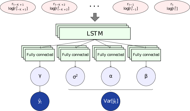
Figure 1: Input sequence (shaded in red) is passed into one or more LSTM layers. Output from the LSTM layers is then fed into four subnetworks of one or more fully connected layers with ReLU activation. The final layer of each subnetwork is a fully-connected layer with linear activation. Softplus is applied to $\sigma^{2},\alpha$ and $\beta$ to ensure positivity. The four outputs of the neural network are then used to compute $\hat{y}$ and $\operatorname{Var}[\hat{y}]$ (shaded in blue). Note that we can set $\alpha=\beta$, as discussed in Section 3.1. In this case, $\beta$ is dropped and the number of subnetworks reduces from four to three.

For the main application of this work, UQ of financial time-series forecasts, we propose a novel architecture for the modelling of distribution parameters, as illustrated in Figure 1. To predict $\hat{y}_{t}$, time-series inputs of both returns ($r_{t-K+1},\dots,r_{t}$) and log-transformed squared returns ($\log[r_{t-K+1}^{2}],\dots,\log[r_{t}^{2}]$) are fed into one or more long short-term memory (LSTM) layers (Hochreiter and Schmidhuber,, 1997). We log-transform squared returns to reduce skewness. The LSTM layers convert each time-series into a latent representation. The latent representation is then fed into four subnetworks, where each subnetwork is comprised of one or more fully connected layers and applies non-linear transformations on the latent representation. This allows the network to model complex relationships between the parameters in $\bm{\zeta}$ and the sequence. As noted in Section 3.1, we can set $\alpha=\beta$ and reduce the number of subnetworks to three. In other words, the network architecture illustrated in Figure 1 can be modified to output three parameters: $\bm{\zeta}=(\gamma,\sigma^{2},\alpha)$. We have kept $\beta$ to be comparable to Evidential but provide empirical results in Appendix B using the UCI dataset (the same benchmark dataset used in Lakshminarayanan et al.,, 2017 and Amini et al.,, 2020, and discussed in Appendix A.1) to show that the two networks are indeed equivalent. In the following, we explore the proposed design of the architecture in detail.

Lakshminarayanan et al., (2017) and Amini et al., (2020) introduced the Gaussian and NormalInverseGamma layers as the final layer of a neural network. These final layers output parameters of the posterior distribution. Let $\bm{a}\in\operatorname{\mathbb{R}}^{H^{(I)}}$ be the input vector of the final layer with $H^{(I)}$ dimensions and $H^{(O)}$ be the dimension of the output layer. In the case of the NormalInverseGamma layer, $H^{(O)}=4$. The NormalInverseGamma layer outputs,

$$\bm{\zeta}=\mathrm{O}(\bm{a};\bm{\theta})=\bm{a}^{\mkern-1.5mu\mathsf{T}}\cdot\bm{W}^{(O)}+\bm{b}^{(O)}$$

$$\gamma=\zeta_{1},\quad\nu=\zeta_{2},\quad\alpha=\zeta_{3},\quad\beta=\zeta_{4},$$ (16)

where $\mathrm{O}$ denotes the NormalInverseGamma output layer, $\{\zeta_{1,\dots,4}\}$ are 1, …, 4 elements of vector $\bm{\zeta}$, $\bm{W}^{(O)}\in\operatorname{\mathbb{R}}^{H^{(I)}\times H^{(O)}}$ and $\bm{b}^{(O)}\in\operatorname{\mathbb{R}}^{H^{(O)}}$ are weights and bias of the output layer, respectively. Each dimension of $\bm{\zeta}$ corresponds to each of $\gamma,\nu,\alpha$ and $\beta$.

Outputs of the NormalInverseGamma layer are linear transformations of a common input $\bm{a}$ (Equation (16)). We argue that this construct is too restrictive for complex applications, such as in quantifying uncertainty of financial time-series forecasts, as detailed in Section 4.1. We propose to model each of the four parameters of SMD with a fully connected subnetwork of one or more layers. This allows for a more expressive modelling of $\bm{\zeta}$, where each parameter may have complex, non-linear relationships with the input.

Additionally, we enforce constraints on $\sigma^{2}>0$, $\alpha>1$ and $\beta>0$ by applying softplus transformation with a constant term, $z^{\prime}=\log(1+\exp(z))+c$, where $z\in\{\sigma^{2},\alpha,\beta\}$ and $c$ is the minimum value of the respective parameters. The transformed values constitute the final output of the network: $\bm{\zeta}^{\prime}=\{\gamma,(\sigma^{2})^{\prime},\alpha^{\prime},\beta^{\prime}\}$. In Section 4.1, we show that this modification vastly improves quantification of forecast uncertainty of financial time-series. For other network architectures, we argue that the same approach can be applied. In the case of a feedforward network, we recommend having at least one common hidden layer that reduces the input to a single latent representation. The latent representation is then passed to individual subnetworks for specialization. We argue that the common hidden layer allows information sharing across the four parameters, while having no common hidden layer (i.e., if the input is fed into the four disjoint stacks of hidden layers directly) will prevent sharing of information across the stacks.

Machine learning models are typically trained using pooled dataset of historical observations. As such, they learn the average uncertainty within the historical data. However, as noted in Section 1, asset returns exhibit time-varying volatility clustering patterns. Thus, we expect predictive uncertainty to be correlated with time-varying variance of the DGP. In other words, predictive uncertainty is high when $\sigma_{t}^{2}$ of the DGP is high and the model is “surprised” by the volatility. To inform the neural network of the prevailing volatility environment, we propose to include the log of squared returns $\{\log(r_{t-K+1}^{2}),\dots,\log(r_{t}^{2})\}$ as part of the input matrix. This follows from the use of squared returns in volatility forecasting literature (Brownlees et al.,, 2011) and allows the neural network to infer the prevailing volatility environment.

Model averaging, as a special case of ensembling, is a well studied statistical method for improving predictive power of estimators (Breiman,, 1996; Goodfellow et al.,, 2016), and has previously been shown to improve accuracy of financial time-series forecasting (Wong et al.,, 2021) and sequential predictions (Raftery et al.,, 2010). As accuracy of both return forecast accuracy and predictive uncertainty are important in our motivating application, we propose to incorporate model averaging to improve return forecasts at the cost of higher predictive uncertainty estimates. For an ensemble of $M$ models, we compute the ensemble forecast $\tilde{y}$ and predictive variance $\operatorname{Var}[\tilde{y}]$ as,

$$\tilde{y}=\frac{1}{M}\sum_{i=1}^{M}\hat{y}_{i},\quad\operatorname{Var}[\tilde{y}]=\frac{1}{M}\sum_{i=1}^{M}(\hat{y}_{i}^{2}+\operatorname{Var}[\hat{y}_{i}])-\tilde{y}^{2},$$ (17)

where $\hat{y}_{i}$ and $\operatorname{Var}[\hat{y}_{i}]$ are mean and predictive variance of model $i$, respectively. In Equation (17), $\operatorname{E}[\hat{y}^{2}]>\operatorname{E}[\hat{y}]^{2}$ (by Jensen’s inequality). Thus, predictive uncertainty of the ensemble will be higher than estimated using the marginal t-distribution alone. In Section 4, we show that model averaging resulted in significant predictive performance improvement and, despite the higher uncertainty estimates, resulted in the lowest NLL.

Popular tools for modelling time-varying volatility are Autoregressive Conditional Heteroskedasticity (ARCH; Engle,, 1982) and GARCH models. GARCH, when applied to stock returns, assumes the same DGP as Equation (1). Time-varying variance $\sigma_{t}^{2}$ is modelled using an ARMA model (Box et al.,, 1994). Parameter $\mu_{t}$ can assume a fixed value (e.g., sample mean or 0) or modelled using time-series models such as ARMA (leading to the ARMA-GARCH formulation). In our proposed framework, squared returns are provided as inputs to LSTM in similar spirit to the autoregressive terms of squared returns in GARCH. However, our proposed framework also has few differences to ARMA-GARCH. A neural network offers greater flexibility in modelling and can automatically discover interaction effects between returns and volatility. For example, higher volatility is negatively correlated with future asset returns (known as the leverage effect; Cont,, 2001). By contrast, modelling of interaction effects in additive models (such as GARCH) requires explicit specification by the user. LSTM can also be interpreted as having dynamic autoregressive orders (as opposed to fixed orders in GARCH). The input and forget gates of LSTM allow the network to control the extent of long-memory depending on features of the time-series. Multi-step ahead forecasting is an iterative process for ARMA-GARCH and forecast errors may compound. LSTM is able to predict multi-step ahead directly. In Section 4.1, we apply our framework to forecast forward 1-month U.S. stock returns using daily returns. Nonetheless, we do not directly compare against ARMA-GARCH models for two reasons. First, in this work, we are focused on advancing UQ methodologies for neural networks. We argue that several of our advances can be beneficial to both time-series and non-time-series datasets (as demonstrated in Appendix A.1). Second, we lean on the plethora of literature in comparing LSTM to ARMA-variants (e.g., Siami-Namini et al.,, 2018) and ARCH-variants (e.g., Liu,, 2019).

For ease of comparison, we outline the differences of our method to Ensemble (Lakshminarayanan et al.,, 2017) and Evidential (Amini et al.,, 2020) in Table 1.

Table 1: A comparison of Combined to Deep Ensemble and Deep Evidential regressions. Output layer refers to the structure of output layer(s) of the network that outputs the parameters of the likelihood function.

Method	Ensemble	Evidential	Combined
Prior	None	NIG	Gamma
Ensemble	Yes	No	Yes
Likelihood	Gaussian	Student’s t	Student’s t
Output layer	Single layer $\mu,\sigma^{2}$	Single layer $\gamma,\nu,\alpha,\beta$	Multi-layer $\gamma,\sigma^{2},\alpha,\beta$

4 Experiments

Our proposed framework is primarily focused on advancing UQ in time-series exhibiting volatility clustering. In this section, we detail experiment results in our motivating application — time-series forecasting and UQ on cryptocurrency and U.S. equities time-series datasets, to illustrate the benefits of our proposed method. Nonetheless, SMD parameterization, modelling distribution parameters using subnetworks and ensemble predictions can also be applied to general applications of prediction UQ. In Appendix A.1, we also compare our method to Ensemble and Evidential using the UCI benchmark dataset. This is intended to provide readers with a direct comparison to the results published in Lakshminarayanan et al., (2017) and Amini et al., (2020), demonstrating the benefits of our proposed improvements in non-time-series datasets.

4.1 Uncertainty quantification in financial time-series forecasting

In this section, we will first describe the cryptocurrency dataset, then the U.S. equities dataset. The same neural network architectures are used in the two datasets, with hyperparameters tuned independently. Our cryptocurrency dataset consists of hourly returns downloaded from Binance over July 2018 to December 2021, for 10 of the most liquid, non-stablecoin cryptocurrencies. Tickers for these cryptocurrencies are BTC, ETH, BNB, NEO, LTC, ADA, XRP, EOS, TRX and ETC, denominated in USDT. Following Ambachtsheer, (1974), Grinold and Kahn, (1999) and Wong et al., (2021), we use mean cross-sectional correlation ($\tfrac{1}{T}\sum_{t=1}^{T}\rho(\bm{y}_{t},\hat{\bm{y}_{t}})$, where $\bm{y}_{t}$ and $\hat{\bm{y}_{t}}$ are vectors of prediction and target at $t$ for all 10 cryptocurrencies) as a measure of predictive accuracy, in addition to RMSE and NLL. Data from July 2018 to June 2019 are used for hyperparameter tuning, chronologically split into $70\text{\,}\mathrm{\char 37\relax}$ training and $30\text{\,}\mathrm{\char 37\relax}$ validation. Data from July 2019 to December 2021 are used for out-of-sample testing. Networks are trained every 30 days using an expanding window of data from July 2018. Each input sequence consists of 10 days of hourly returns $r$ and squared returns $\log(r^{2})$ (i.e., the input is a matrix with dimensions $240\times 2$), and are used to predict forward one hour return (i.e., units of analysis and observation are both hourly). This training scheme is shared across all three models. Network topology consists of LSTM layers, followed by fully connected layers with ReLU activation and the respective output layers of Ensemble (Gaussian) and Evidential (NormalInverseGamma). For Combined, we use four separate subnetworks as illustrated in Figure 1. As discussed in Section 1, we consider UQ in cryptocurrencies to be especially challenging due to their high volatility. Note that in this section, “forecast uncertainty” and “uncertainty forecast” refer to estimated predictive uncertainty (i.e., sum of epistemic and aleatoric uncertainties) for simplicity.

Our U.S. equities experiment follows the same setup as cryptocurrencies. Mimicking the S&P 500 index universe, the dataset consists of daily returns downloaded from the Wharton Research Data Service over 1984 to 2020, for the 500 largest stocks listed on NASDAQ, NYSE and NYSE American. Data from 1984 to 1993 are used for hyperparameter tuning, while 1994 to 2020 are used for out-of-sample testing. The network is refitted every January using a rolling 10-year window. Each input sequence consists of 240 trading days (approximately one-year) of daily returns $r$ and squared returns $\log(r^{2})$, forecasting forward 20-day (approximately one-month) return and its uncertainty. Note that the unit of analysis is monthly and unit of observation is daily. One-month is a popular forecast horizon for U.S. equities in literature (e.g., Gu et al.,, 2020 and Wong et al.,, 2021), which motivated our choice of forecast horizon.

At this point, it is useful to remind readers that prior literature have found both datasets to exhibit time-varying variance (e.g., Cont,, 2001; Hafner,, 2018), which is also visible in Figure 2. We start with the main empirical results of this work. Table 2 contains forecast results on both the cryptocurrency dataset (left) and U.S. equities (right). We observe that Combined has the highest average cross-sectional correlation (higher is better), and lowest RMSE and NLL (both lower is better) in both datasets. This indicates that Combined has higher cross-sectional predictive efficacy (as measured by correlation) and is able to better forecast uncertainty of the time-series prediction. Evidential has higher (better) correlation and lower RMSE (better) than Ensemble but higher (worse) NLL in cryptocurrency. In U.S. equities, Evidential has worse correlation, RMSE and NLL than Ensemble. Correlations in U.S. equities are materially lower for all three methods compared to the cryptocurrency dataset. We hypothesize that this is due to both the difference in forecast horizon and maturity of the U.S. stock market.

Table 2: Main results: Comparing Ensemble, Evidential and Combined on average cross-sectional correlation, RMSE and NLL for cryptocurrencies (left) and U.S. equities (right), respectively. Average result and standard deviation over 10 trials for each method. Best method for each dataset is highlighted in bold.

Cryptocurrency U.S. equities Metric Ensemble Evidential Combined Ensemble Evidential Combined Correlation ($\times 100$) $2.78\pm 1.09$ $3.94\pm 1.84$ $\bm{9.87\pm 3.17}$ $0.40\pm 0.66$ $0.09\pm 0.93$ $\bm{1.22\pm 0.65}$ RMSE ($\times 100$) $0.874\pm 0.022$ $0.874\pm 0.003$ $\bm{0.867\pm 0.001}$ $9.426\pm 0.044$ $9.433\pm 0.033$ $\bm{9.379\pm 0.020}$ NLL $-3.74\pm 0.10$ $-3.24\pm 0.02$ $\bm{-4.14\pm 0.01}$ $-1.65\pm 0.17$ $-0.82\pm 0.03$ $\bm{-1.71\pm 0.01}$

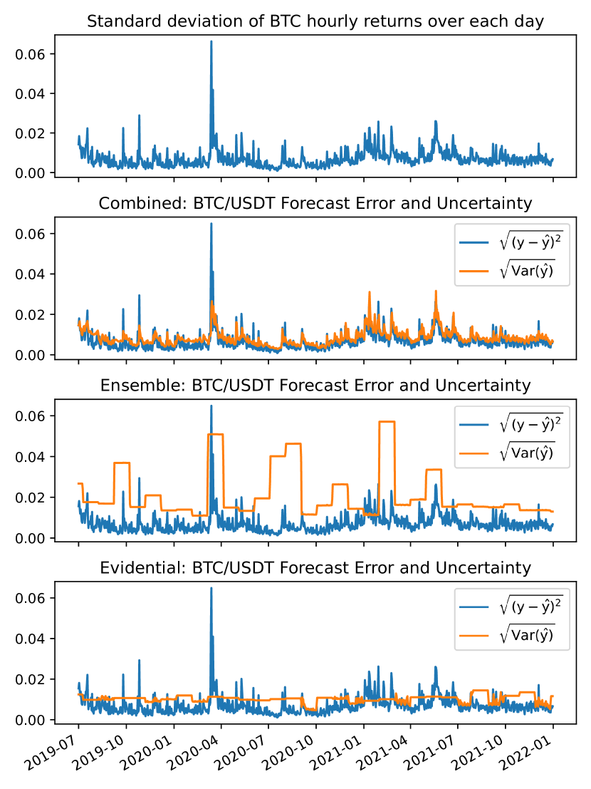
(a) Uncertainty of Bitcoin

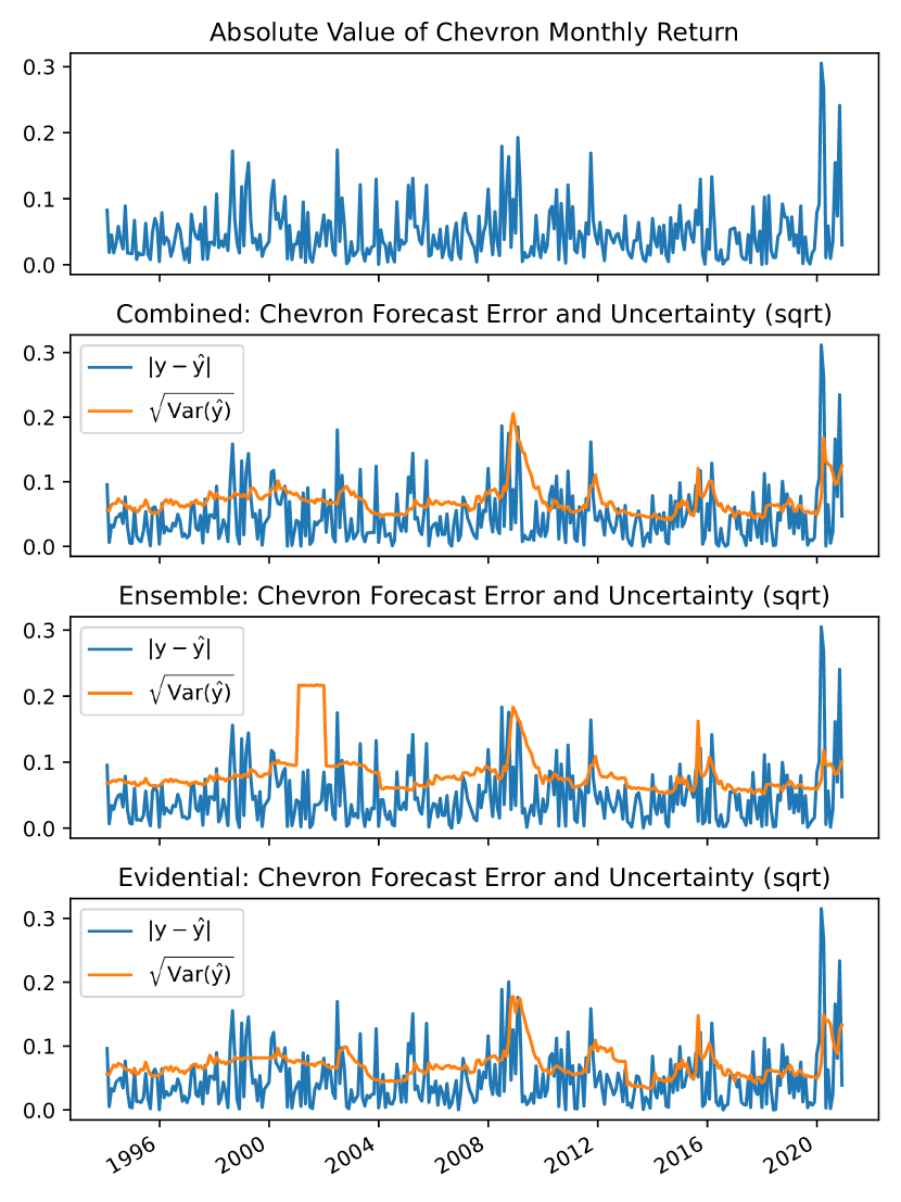
(b) Uncertainty of Chevron

Figure 2: Forecast uncertainties of Combined, Ensemble and Evidential applied to Bitcoin (left) and Chevron Corp (right), respectively. For Bitcoin, square root of the average over each day shown.

Next, Figure 2 compares predicted uncertainty and actual prediction error of the three methods to actual volatility of Bitcoin (BTC/USDT), the cryptocurrency with the highest market capitalization, and Chevron Corp., a major U.S. oil producer which have endured multiple market shocks. Volatility forecasts are often compared with observed volatility (typically computed over a look back window) to evaluate forecast performance. However, the true instantaneous volatility of an asset (i.e., $\sigma^{2}$ in Equation (1)) is unobservable (Ge et al.,, 2022). Thus, in the top row of Figure 2, we use the standard deviation of hourly returns computed over each day for Bitcoin and absolute value of monthly returns for Chevron (as forecast horizon is monthly), as proxies for $\sigma^{2}$. In rows 2–4, for Bitcoin, we aggregate hourly forecasts to daily data points by computing the daily root mean squared return forecast error $\sqrt{\tfrac{1}{24}\sum_{k=0}^{23}(y_{t-k}-\hat{y}_{t-k})^{2}}$ (denoted $\sqrt{(y-\hat{y})^{2}}$) computed from hourly return forecasts, and the daily root mean predictive uncertainty $\sqrt{\tfrac{1}{24}\sum_{k=0}^{23}\operatorname{Var}(\hat{y}_{t-k})}$ (denoted $\sqrt{\operatorname{Var}(\hat{y})}$), for each $t=24,48,72,\dots,T$ (note that $t$ for cryptocurrency is in hourly units). For Chevron, as the unit of analysis is monthly, we plot the absolute error between actual monthly returns and predicted returns (denoted $|y-\hat{y}|$), and square-root of forecast uncertainty (denoted $\sqrt{\operatorname{Var}(\hat{y})}$) on the right column of Figure 2. Comparing the top row of Figure 2 to the root return forecast error of row 2-4 (blue line), we observe that forecast error spikes when volatility of the asset spikes. This is expected, as the spike in volatility leads to large forecast errors. Comparing the bottom three rows of Figure 2, which correspond to Combined, Ensemble and Evidential, respectively. We observe that Combined’s predicted uncertainty of $\hat{\mu}$ tracks actual forecast error much more closely than Evidential and Ensemble. This appears to be especially true during periods of elevated volatility, which are important to investors. Overestimation of predictive uncertainty is severe for Ensemble in Bitcoin, where predictive uncertainty can sometimes be significantly higher than observed forecast error. Lastly, Evidential underestimates forecast error during heightened volatility (e.g., March 2020 in Figure 2) and overestimates forecast error under periods of low volatility (e.g., July 2020 in Figure 2).

For Chevron, we observe multiple spikes of volatility, corresponding to the U.S. recession over 2008-09, the oil shock in 2015 and the 2020 pandemic. Notably, we observe that Combined tracks the spike in forecast error better than Ensemble and Evidential. Note that the “block-like” appearances of uncertainty forecasts of both Ensemble and Evidential are due to periodic training (monthly for cryptocurrencies and yearly for U.S. equities) and the failure to generalize the prevailing volatility environment. During training, the optimizer updates network weights $\bm{W}$ and bias $\bm{b}$ (which is analogous to the intercept in linear models). When the network fails to generalize, it minimizes the loss function by updating the bias rather than the weights. Thus, outputting the same constant that do not vary with the input, until the network is re-trained in the following month (for cryptocurrencies) or year (for U.S. equities). This produces the block-like appearances of Ensemble and Evidential, and is indicative of the network setup (e.g., no separate modelling of hyperparameters) being unsuitable to this class of problems. We observe similar visual characteristics in the predicted uncertainty of other cryptocurrencies and stocks.

4.2 Ablation study

Table 3: Ablation studies of Combined: In each column, we remove model averaging (No Averaging), separate modelling of distribution parameters (Single Output) and using return time-series only (Returns-only) for cryptocurrencies (left) and U.S. equities (right), respectively. Average result and standard deviation over 10 trials for each method. Note that cryptocurrency returns are hourly and U.S. stock returns are monthly.

Cryptocurrency U.S. equities Metric No Averaging Single Output Returns-only No Averaging Single Output Returns-only Correlation ($\times 100$) $4.48\pm 2.80$ $8.23\pm 2.91$ $10.46\pm 2.04$ $0.92\pm 0.65$ $1.87\pm 1.06$ $1.21\pm 0.73$ RMSE ($\times 100$) $0.868\pm 0.001$ $0.872\pm 0.002$ $0.866\pm 0.002$ $9.392\pm 0.020$ $9.398\pm 0.029$ $9.384\pm 0.046$ NLL $-3.35\pm 0.01$ $-4.04\pm 0.02$ $-3.95\pm 0.02$ $-0.88\pm 0.01$ $-1.63\pm 0.04$ $-1.34\pm 0.04$

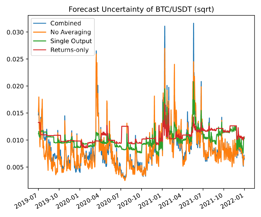
(a) Uncertainty of Bitcoin

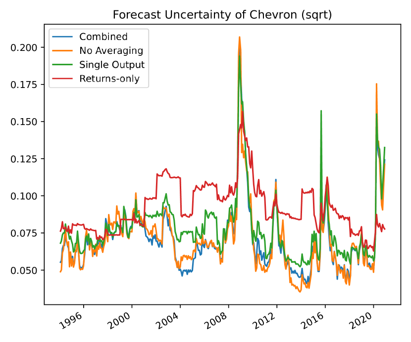
(b) Uncertainty of Chevron

Figure 3: Predicted uncertainty $\operatorname{Var}(\hat{y})$ of Combined, omitting each of model averaging (Averaging), single output layer (Single Output) and using returns only (Returns-only) for BTC/USDT and Chevron.

Next, we test the effects of removing each of the following for Combined: 1) model averaging; 2) single output layer for all distribution parameters (same as Evidential); 3) using return time-series only (i.e., no squared returns). The results are recorded in Table 3 and in Figure 3. As discussed in Section 3.2, model averaging (Equation (17)) will lead to higher predictive uncertainty estimates. In Table 3, we observe that omitting model averaging has a large negative impact on cross-sectional correlation and NLL. Cross-sectional correlation is $55\text{\,}\mathrm{\char 37\relax}$ and $25\text{\,}\mathrm{\char 37\relax}$ lower for cryptocurrencies and U.S. equities, respectively. While NLL is higher by 0.8 in both cases (lower is better), indicating a worse overall fit. However, it does not appear to impede the network’s ability to model time-series forecast uncertainty. Moreover, comparing Combined (with model averaging) to No Averaging (without model averaging) in Figure 3, we observe very similar estimated predictive uncertainties with and without model averaging (as the orange and blue lines track each other closely). This indicates a favorable trade-off between significantly improved forecast performance and practically the same predictive uncertainty estimates. Using a single output layer for all distribution parameters leads to marginally worse NLL. Correlation is lower in cryptocurrencies but marginally higher in U.S. equities. While using returns only leads to marginally higher correlation but marginally worse on NLL in cryptocurrency, and lower correlation and worse NLL in U.S. equities. From Figure 3, the block-like appearances indicate that both using single output layer and using returns only result in the network failing to closely track time-varying variance of the DGP. This suggests that both squared returns and separate modelling of distribution parameters are required to model time-varying forecast uncertainty.

5 Conclusions

Our motivating application of portfolio selection depends on both forecasts and forecast uncertainties. This is a challenging problem due to both the low signal-to-noise ratio in financial markets (Gu et al.,, 2020) and the presence of volatility clustering. To this end, we present a method for the simultaneous forecasting asset returns and modelling of forecast uncertainty in presence of volatility clustering. Our proposed method extends and simplifies the work of Lakshminarayanan et al., (2017) and Amini et al., (2020). We propose to use a SMD (which uses a Gamma prior for scale uncertainty $\nu$) as a simpler alternative to a NIG prior, in which a Normal prior is placed on $\mu$ and an Inverse-Gamma prior on $\sigma^{2}$). Parameters of SMD are modelled using separate subnetworks. Together with ensembling and the use of second order of returns as inputs, we show that our proposed method can successfully model time-varying variance of the DGP, while providing superior forecasting performance than two state-of-the-art neural network UQ methods — Evidential and Ensemble. This is illustrated through the successful quantification of forecast uncertainty of two financial time-series datasets: cryptocurrency and U.S. equities.

Our proposed SMD formulation offers an avenue to resolve some of the criticisms of Meinert et al., (2022) and Bengs et al., (2023). In particular, our SMD parameterization has three effective parameters and thus does not have any unresolved degrees of freedom. We can set $\alpha=\beta$, which leads to a marginal t-distribution where the three distributional parameters ($\gamma,\sigma^{2},\alpha$) relate directly to the location, scale and shape of the t-distribution, without the need of a hierarchical model. In this formulation, epistemic uncertainty is assumed to be the difference between the predictive (t-distributed) and aleatoric (Normal-distributed) uncertainties. This assumption provides for a simpler model but lacks the granular attribution between aleatoric and epistemic uncertainties afforded by the NIG prior in Evidential. However, as Meinert et al., (2022) has pointed out, the granular control comes at the cost of an unresolved degree of freedom. Thus, users are encouraged to weigh the trade-offs in choosing a method to deploy. This also makes for a potential future research direction. We show empirically that our method is able to accurately predict forecast errors, similar to the success Evidential demonstrated in other real world applications (e.g., see Liu et al.,, 2021; Soleimany et al.,, 2021; Cai et al.,, 2021; Singh et al.,, 2022; Li and Liu,, 2022). From a finance application perspective, forecast uncertainty can be used to size bets, or as advanced warning to protect the portfolio from downside risk. For example, if forecast uncertainty reaches a certain threshold, an investor could purchase portfolio insurance (e.g., put options) or liquidate positions to reduce risk. The ability to attribute epistemic and aleatoric uncertainties may also allow for more advanced portfolio optimization techniques to be developed in future research (e.g., place different risk aversions on the two sources of uncertainties). Lastly, UQ in time-series applications is a relatively under-explored area of literature. We believe this work can lead to further advancements of UQ in complex time-series.

Appendix A Marginal distribution of a Scale Mixture

From Equation (10), we have $\operatorname{N}(y|\gamma,\tfrac{\sigma^{2}}{\lambda})\operatorname{Gam}(\lambda|\alpha,\beta)$. Marginalizing over $\lambda$ produces the data likelihood,

$$\mathrm{p}(y|\gamma,\sigma^{2},\alpha,\beta) =\int_{\lambda}^{\infty}\mathrm{p}_{\operatorname{N}}(y|\gamma,\sigma^{2}\lambda^{-1})\mathrm{p}_{\operatorname{G}}(\lambda|\alpha,\beta)\mathop{}\!\mathrm{d}\lambda$$

$$=\int_{\lambda}^{\infty}\left[\sqrt{\frac{\lambda}{2\pi\sigma^{2}}}\exp\left\{-\frac{\lambda(y-\gamma)^{2}}{2\sigma^{2}}\right\}\right]\left[\frac{\beta^{\alpha}}{\Gamma(\alpha)}\lambda^{\alpha-1}\exp^{-\beta\lambda}\right]\mathop{}\!\mathrm{d}\lambda$$

$$=\frac{\beta^{\alpha}}{\Gamma(\alpha)\sqrt{2\pi\sigma^{2}}}\int_{\lambda=0}^{\infty}\lambda^{\alpha-\tfrac{1}{2}}\exp\left\{-\frac{\lambda(y-\gamma)^{2}}{2\sigma^{2}}-\beta\lambda\right\}\mathop{}\!\mathrm{d}\lambda$$

$$=\frac{\beta^{\alpha}}{\Gamma(\alpha)\sqrt{2\pi\sigma^{2}}}\left[\frac{(y-\gamma)^{2}}{2\sigma^{2}}+\beta\right]^{-(\alpha+\tfrac{1}{2})}\int_{\lambda=0}^{\infty}\left\{\lambda\left[\frac{(y-\gamma)^{2}}{2\sigma^{2}}+\beta\right]\right\}^{\alpha-\tfrac{1}{2}}$$

$$\quad\exp\left\{-\lambda\left[\frac{(y-\gamma)^{2}}{2\sigma^{2}}+\beta\right]\right\}\mathop{}\!\mathrm{d}\left\{\lambda\left[\frac{(y-\gamma)^{2}}{2\sigma^{2}}+\beta\right]\right\},$$

since $\int_{0}^{\infty}x^{\alpha-1}\exp(-x)\mathop{}\!\mathrm{d}x=\Gamma(\alpha)$,

$$=\frac{\beta^{\alpha}}{\sqrt{2\pi\sigma^{2}}}\frac{\Gamma(\alpha+\tfrac{1}{2})}{\Gamma(\alpha)}\left[\frac{(y-\gamma)^{2}}{2\sigma^{2}}+\beta\right]^{-(\alpha+\tfrac{1}{2})}\hskip 54.06023pt$$

and re-arranging $\beta^{\alpha}=(\tfrac{1}{\beta})^{-\alpha}=(\tfrac{1}{\beta})^{-(\alpha+\tfrac{1}{2})+\tfrac{1}{2}}$,

$$=\frac{\Gamma(\alpha+\tfrac{1}{2})}{\Gamma(\alpha)}\frac{1}{\sqrt{2\pi\sigma^{2}\beta}}\left[\frac{(y-\gamma)^{2}}{2\sigma^{2}\beta}+1\right]^{-(\alpha+\tfrac{1}{2})}\hskip 119.50157pt$$

$$\mathrm{p}(y|\gamma,\sigma^{2},\alpha,\beta) =\operatorname{St}\left(y;\gamma,\frac{\sigma^{2}\beta}{\alpha},2\alpha\right).$$ (18)

To show that the last step of Equation (18) is true, we start with the probability density function of the t-distribution parameterised in terms of precision $\operatorname{St}(y|\gamma,b^{-1},a)$ (Bishop,, 2006),

$$\operatorname{St}(y|\gamma,b^{-1},a) =\frac{\Gamma(\tfrac{a+1}{2})}{\Gamma(\tfrac{a}{2})}\left[\frac{b}{\pi a}\right]^{\tfrac{1}{2}}\left[1+\frac{b(y-\gamma)^{2}}{a}\right]^{-(\tfrac{a+1}{2})},$$

where $\gamma$ is location, $b$ is inverse of scale and $a$ is shape. Substituting in $b^{-1}=\tfrac{\sigma^{2}\beta}{\alpha}$ and $a=2\alpha$,

$$\operatorname{St}\left(y|\gamma,\frac{\sigma^{2}\beta}{\alpha},2\alpha\right) =\frac{\Gamma(\alpha+\tfrac{1}{2})}{\Gamma(\alpha)}\left[\frac{(\tfrac{\alpha}{\sigma^{2}\beta})}{2\pi\alpha}\right]^{\tfrac{1}{2}}\left[1+\frac{\alpha(y-\gamma)^{2}}{2\sigma^{2}\alpha\beta}\right]^{-(\alpha+\tfrac{1}{2})}$$

$$=\frac{\Gamma(\alpha+\tfrac{1}{2})}{\Gamma(\alpha)}\frac{1}{\sqrt{2\pi\sigma^{2}\beta}}\left[\frac{(y-\gamma)^{2}}{2\sigma^{2}\beta}+1\right]^{-(\alpha+\tfrac{1}{2})}.$$

From Equation (18), the NLL of the marginal t-distribution is,

$$\mathrm{p}(y|\gamma,\sigma^{2},\alpha,\beta) =\frac{\Gamma(\alpha+\tfrac{1}{2})}{\Gamma(\alpha)}\frac{1}{\sqrt{2\pi\sigma^{2}\beta}}\left[\frac{(y-\gamma)^{2}}{2\sigma^{2}\beta}+1\right]^{-(\alpha+\tfrac{1}{2})}$$

$$-\log[\mathrm{p}(y|\gamma,\sigma^{2},\alpha,\beta)] =\log\left[\frac{\Gamma(\alpha)}{\Gamma(\alpha+\tfrac{1}{2})}\right]+\tfrac{1}{2}\log[2\pi\sigma^{2}\beta]+(\alpha+\tfrac{1}{2})\log\left[\frac{(y-\gamma)^{2}}{2\sigma^{2}\beta}+1\right].$$

A.1 Benchmarking on UCI dataset

Table 4: Comparing Ensemble (Lakshminarayanan et al.,, 2017), Evidential (Amini et al.,, 2020) and Combined (this work) on RMSE and NLL using the UCI benchmark datasets. Average result and standard deviation over 5 trials for each method. The best method for each dataset and metric are highlighted in bold.

	RMSE			NLL
Dataset	Ensemble	Evidential	Combined	Ensemble	Evidential	Combined
Boston	$\bm{2.66\pm 0.20}$	$2.95\pm 0.29$	$2.89\pm 0.31$	$2.28\pm 0.05$	$2.30\pm 0.05$	$\bm{2.23\pm 0.05}$
Concrete	$5.79\pm 0.16$	$5.98\pm 0.23$	$\bm{5.40\pm 0.18}$	$3.07\pm 0.02$	$3.11\pm 0.04$	$\bm{2.98\pm 0.03}$
Energy	$1.86\pm 0.04$	$1.84\pm 0.06$	$\bm{1.71\pm 0.20}$	$1.36\pm 0.02$	$1.41\pm 0.04$	$\bm{1.35\pm 0.05}$
Kin8nm	$\bm{0.06\pm 0.00}$	$0.06\pm 0.00$	$0.06\pm 0.00$	$\bm{-1.39\pm 0.02}$	$-1.28\pm 0.03$	$-1.35\pm 0.02$
Naval	$\bm{0.00}\pm 0.00$	$0.00\pm 0.00$	$0.00\pm 0.00$	$\bm{-6.10\pm 0.05}$	$-5.99\pm 0.09$	$-5.89\pm 0.35$
Power	$3.02\pm 0.09$	$3.02\pm 0.08$	$\bm{2.95\pm 0.08}$	$2.57\pm 0.01$	$2.56\pm 0.03$	$\bm{2.53\pm 0.02}$
Protein	$3.71\pm 0.10$	$4.28\pm 0.23$	$\bm{3.67\pm 0.13}$	$\bm{2.61\pm 0.03}$	$2.73\pm 0.08$	$2.70\pm 0.05$
Wine	$0.60\pm 0.03$	$\bm{0.56\pm 0.02}$	$0.59\pm 0.03$	$0.94\pm 0.04$	$\bm{0.92\pm 0.04}$	$1.00\pm 0.03$
Yacht	$\bm{1.22\pm 0.22}$	$1.48\pm 0.47$	$3.97\pm 1.06$	$1.06\pm 0.08$	$\bm{0.96\pm 0.19}$	$1.17\pm 0.11$

In this section, we compare our method to Ensemble and Evidential using the UCI benchmark dataset. This is intended to provide readers with a direct comparison to Lakshminarayanan et al., (2017) and Amini et al., (2020) on the same dataset used in both works. The collection consists of nine real world regression problems, each with 10–20 features and hundreds to tens of thousands of observations. We note the Wine dataset within UCI contains discrete values (ratings of wine characteristics, such as color and taste) which may render the assumption of a continuous, symmetrical data distribution less appropriate if these values are skewed. More recently, larger UQ datasets have been published in Dheur and Ben Taieb, (2023), which may be useful in assessing the state-of-the-art in non-time-series UQ methods. We follow Lakshminarayanan et al., (2017) and Amini et al., (2020) in evaluating our method on root mean squared error (RMSE, which assesses forecast accuracy) and NLL (which assesses overall distributional fit), and compare against Ensemble and Evidential. While we do not explicitly compare inference speed, as our Combined method also uses ensembling, inference speed is expected to be comparable to Ensemble while being slower than Evidential. We use the source code provided by Amini et al., (2020), with the default topology of a single hidden layer with 50 units for both Ensemble and Evidential. For Combined, as individual modelling of distribution parameters (Section 3.2) requires a network with two or more hidden layers, we have used a single hidden layer with 24 units, followed by 4 separate stacks of a single hidden layer with 6 units each. Thus, the total number of non-linear units is 48 (compared to 50 for Ensemble and Evidential). Note that even though the total number of units are similar across the three models, learning capacity may differ due to different topologies.

Table 4 records experiment results on the UCI dataset. On RMSE, we find that both Ensemble and Combined have performed well, having the best RMSE in four datasets each. In two of the sets (Kin8nm and Naval), all three methods produced highly accurate results that are not separable to two decimal points. Turning to NLL, we observe a trend towards Combined having lower NLL than the other two methods for four sets, followed by Ensemble with three sets. Comparing Combined to Evidential, we find that Combined generally has lower RMSE (7 of 9 sets) and NLL (6 of 9 sets). Although our method is designed for UQ of complex time-series and all 9 datasets are pooled (non-time-series) datasets, we still observe some improvements in both RMSE and NLL.

Next, we present further ablation studies on the UCI dataset. Table 5 records results of Alternative, which utilizes ensembling and SMD parameterization but not separate modelling of hyperparameters. Alternative has the same network topology as Ensemble and Evidential (a single hidden layer with 50 units), as opposed to Combined which has two hidden layers with a total of 48 units. We observe that Ensemble has the lowest RMSE in 5 (of 9) datasets, followed by Alternative (3 of 9), while Alternative has the best NLL in 6 (of 9) datasets and Ensemble has 3 (of 9). On both metrics, Evidential has the least favourable performance. Comparing Combined in Table 4 and Alternative in Table 5, Combined has lower RMSE and NLL in 5 of 9 datasets. Thus, we conclude that separate modelling of hyperparameters provided an incremental benefit on the UCI datasets.

Table 5: Comparing Ensemble, Evidential and Alternative (without separate modelling of the four parameters of SMD) on RMSE and NLL using the UCI benchmark datasets. Average result and standard deviation over 5 trials for each method. The best method for each dataset and metric is highlighted in bold.

	RMSE			NLL
Dataset	Ensemble	Evidential	Alternative	Ensemble	Evidential	Alternative
Boston	$\bm{2.66\pm 0.20}$	$2.95\pm 0.29$	$2.87\pm 0.18$	$\bm{2.28\pm 0.05}$	$2.30\pm 0.05$	$2.29\pm 0.04$
Concrete	$5.79\pm 0.16$	$5.98\pm 0.23$	$\bm{5.72\pm 0.15}$	$3.07\pm 0.02$	$3.11\pm 0.04$	$\bm{3.03\pm 0.02}$
Energy	$1.86\pm 0.04$	$\bm{1.84\pm 0.06}$	$1.88\pm 0.04$	$1.36\pm 0.02$	$1.41\pm 0.04$	$\bm{1.35\pm 0.03}$
Kin8nm	$\bm{0.06\pm 0.00}$	$0.06\pm 0.00$	$0.06\pm 0.00$	$\bm{-1.39\pm 0.02}$	$-1.28\pm 0.03$	$-1.38\pm 0.02$
Naval	$\bm{0.00\pm 0.00}$	$0.00\pm 0.00$	$0.00\pm 0.00$	$-6.10\pm 0.05$	$-5.99\pm 0.09$	$\bm{-6.12\pm 0.06}$
Power	$3.02\pm 0.09$	$3.02\pm 0.08$	$\bm{2.97\pm 0.10}$	$2.57\pm 0.01$	$2.56\pm 0.03$	$\bm{2.54\pm 0.02}$
Protein	$\bm{3.71\pm 0.10}$	$4.28\pm 0.23$	$3.75\pm 0.11$	$\bm{2.61\pm 0.03}$	$2.73\pm 0.08$	$2.72\pm 0.02$
Wine	$0.60\pm 0.03$	$0.56\pm 0.02$	$\bm{0.55\pm 0.02}$	$0.94\pm 0.04$	$0.92\pm 0.04$	$\bm{0.92\pm 0.02}$
Yacht	$\bm{1.22\pm 0.22}$	$1.48\pm 0.47$	$1.45\pm 0.33$	$1.06\pm 0.08$	$0.96\pm 0.19$	$\bm{0.93\pm 0.09}$

In Table 6, we further remove model averaging. The network used is identical to Evidential but trained using the SMD parameterization (i.e., we simply change the loss function in Evidential to Equation (12)). We observe that the network trained using the SMD parameterization has lower RMSE in 6 of 9 and lower NLL in 8 out 9 datasets. We argue that the improved performance of the SMD parameterization is due to its simplicity.

Table 6: Comparing Normal-Inverse-Gamma and Normal-Gamma on RMSE and NLL using the UCI benchmark datasets. Average result and standard deviation over 5 trials for each method. The best method for each dataset and loss function is highlighted in bold.

	RMSE		NLL
Dataset	NIG	SMD	NIG	SMD
Boston	$\bm{2.95\pm 0.29}$	$2.97\pm 0.20$	$\bm{2.30\pm 0.05}$	$2.31\pm 0.05$
Concrete	$5.98\pm 0.23$	$\bm{5.78\pm 0.23}$	$3.11\pm 0.04$	$\bm{3.05\pm 0.04}$
Energy	$\bm{1.84\pm 0.06}$	$1.87\pm 0.16$	$1.41\pm 0.04$	$\bm{1.33\pm 0.05}$
Kin8nm	$0.06\pm 0.00$	$\bm{0.06\pm 0.00}$	$-1.28\pm 0.03$	$\bm{-1.37\pm 0.01}$
Naval	$0.00\pm 0.00$	$\bm{0.00\pm 0.00}$	$-5.99\pm 0.09$	$\bm{-6.27\pm 0.09}$
Power	$3.02\pm 0.08$	$\bm{2.98\pm 0.12}$	$2.56\pm 0.03$	$\bm{2.53\pm 0.02}$
Protein	$4.28\pm 0.23$	$\bm{3.72\pm 0.16}$	$2.73\pm 0.08$	$\bm{2.39\pm 0.05}$
Wine	$\bm{0.56\pm 0.02}$	$0.56\pm 0.03$	$0.92\pm 0.04$	$\bm{0.87\pm 0.04}$
Yacht	$1.48\pm 0.47$	$\bm{1.44\pm 0.49}$	$0.96\pm 0.19$	$\bm{0.91\pm 0.18}$

Appendix B Further analysis of parameters in a Scale Mixture

In the network architecture proposed in Section 3, output of the network is $\bm{\zeta}=(\gamma,\sigma^{2},\alpha,\beta)$, which parameterises the SMD (Equation (10)). However, as noted in Section 3, we can set $\alpha=\beta$ and reduce the number of parameters to three (Equation (14)). Thus, an alternative specification of the network is to output $\bm{\zeta}=(\gamma,\sigma^{2},\alpha)$ (i.e., three parameters instead of four and are computed through three subnetworks, instead of four in Figure 1). We label this network A=B. In Table 7, we compare Combined (4 parameters) with S2B (3 parameters) using the UCI dataset (as introduced in Section A.1). We observe that A=B is better than Combined on 8 (of 9) datasets on RMSE, while Combined is better than A=B on 1 (of 9). On NLL, A=B is better than Combined on 5 (of 9) datasets, while Combined is better than A=B on 4 (of 9). Even though A=B has a higher number of datasets with lower RMSE and NLL, we note that the differences are very small and are within margin of error (due to randomness in neural network training). Thus, we conclude that the two methods provide near identical results but note that A=B is simpler and more interpretable. However, we choose Combined with four subnetworks to conduct our analysis so that parameters can also be compared with those from Evidential.

Table 7: Comparing A=B (3 parameters) to Combined (4 parameters) on RMSE and NLL using the UCI benchmark datasets. Results are averaged over 5 trials and the best method for each dataset and metric are highlighted in bold.

	RMSE		NLL
Dataset	A=B	Combined	A=B	Combined
Boston	$2.91\pm 0.17$	$\bm{2.89\pm 0.31}$	$2.27\pm 0.04$	$\bm{2.23\pm 0.05}$
Concrete	$\bm{5.39\pm 0.19}$	$5.40\pm 0.18$	$2.99\pm 0.03$	$\bm{2.98\pm 0.03}$
Energy	$\bm{1.56\pm 0.16}$	$1.71\pm 0.20$	$\bm{1.30\pm 0.05}$	$1.35\pm 0.05$
Kin8nm	$\bm{0.06\pm 0.00}$	$0.06\pm 0.00$	$\bm{-1.36\pm 0.02}$	$-1.35\pm 0.02$
Naval	$\bm{0.00\pm 0.00}$	$0.00\pm 0.00$	$-5.87\pm 0.12$	$\bm{-5.89\pm 0.35}$
Power	$\bm{2.93\pm 0.08}$	$2.95\pm 0.08$	$\bm{2.53\pm 0.02}$	$2.53\pm 0.02$
Protein	$\bm{3.60\pm 0.10}$	$3.67\pm 0.13$	$2.83\pm 0.04$	$\bm{2.70\pm 0.05}$
Wine	$\bm{0.57\pm 0.02}$	$0.59\pm 0.03$	$\bm{0.96\pm 0.03}$	$1.00\pm 0.03$
Yacht	$\bm{2.31\pm 0.43}$	$3.97\pm 1.06$	$\bm{1.11\pm 0.09}$	$1.17\pm 0.11$

References

- Ambachtsheer, (1974) Ambachtsheer, K. (1974). Profit potential in an almost efficient market. Journal of Portfolio Management, 1(1):84.
- Amini et al., (2020) Amini, A., Schwarting, W., Soleimany, A., and Rus, D. (2020). Deep evidential regression. In Larochelle, H., Ranzato, M., Raia, Hadsell, Balcan, M.-F., and Lin, H., editors, Advances in Neural Information Processing Systems 33, pages 14927–14937, Vancouver, BC, Canada. Curran Associates, Inc.
- Andrews and Mallows, (1974) Andrews, D. F. and Mallows, C. L. (1974). Scale mixtures of normal distributions. Journal of the Royal Statistical Society: Series B (Methodological), 36(1):99–102.
- Bengs et al., (2023) Bengs, V., Hüllermeier, E., and Waegeman, W. (2023). On second-order scoring rules for epistemic uncertainty quantification. In arXiv.
- Bernardo and Smith, (2000) Bernardo, J. M. and Smith, A. F. M. (2000). Bayesian theory. John Wiley & Sons Ltd.
- Bishop, (2006) Bishop, C. M. (2006). Pattern Recognition and Machine Learning. Springer.
- Black and Litterman, (1991) Black, F. and Litterman, R. B. (1991). Asset allocation: Combining investor views with market equilibrium. Journal of Fixed Income, 1(2):7–18.
- Bollerslev, (1986) Bollerslev, T. (1986). Generalized autoregressive conditional heteroskedasticity. Journal of Econometrics, 31(3):307–327.
- Box et al., (1994) Box, G. E. P., Jenkins, G. M., and Reinsel, G. C. (1994). Time Series Analysis: Forecasting and Control. Prentice Hall, Englewood Cliffs, N.J., USA, 3 edition.
- Breiman, (1996) Breiman, L. (1996). Bagging predictors. Machine Learning, 24(2):123–140.
- Brownlees et al., (2011) Brownlees, C., Engle, R., and Kelly, B. (2011). A practical guide to volatility forecasting through calm and storm. Journal of Risk, 14(2):3–22.
- Byrnes and Barnett, (2018) Byrnes, T. and Barnett, T. (2018). Generalized framework for applying the kelly criterion to stock markets. International Journal of Theoretical and Applied Finance, 21(05):1–13.
- Cai et al., (2021) Cai, P., Wang, H., Huang, H., Liu, Y., and Liu, M. (2021). Vision-based autonomous car racing using deep imitative reinforcement learning. IEEE Robotics and Automation Letters, 6(4):7262–7269.
- Carroll and Kearney, (2009) Carroll, R. and Kearney, C. (2009). GARCH Modeling of Stock Market Volatility, pages 71–90. Chapman & Hall/CRC finance series. CRC Press, New York, NY, USA, 1st edition.
- Charpentier et al., (2021) Charpentier, B., Borchert, O., Zügner, D., Geisler, S., and Günnemann, S. (2021). Natural posterior network: Deep bayesian predictive uncertainty for exponential family distributions. In 9th International Conference on Learning Representations (ICLR), online. OpenReview.net.
- Chen and Hafner, (2019) Chen, C. Y.-H. and Hafner, C. M. (2019). Sentiment-induced bubbles in the cryptocurrency market. Journal of Risk and Financial Management, 12(2):1–12.
- Choy and Chan, (2008) Choy, S. B. and Chan, J. S. (2008). Scale mixtures distributions in statistical modelling. Australian & New Zealand Journal of Statistics, 50(2):135–146.
- Cont, (2001) Cont, R. (2001). Empirical properties of asset returns: stylized facts and statistical issues. Quantitative Finance, 1:223–236.
- Dheur and Ben Taieb, (2023) Dheur, V. and Ben Taieb, S. (2023). A large-scale study of probabilistic calibration in neural network regression. In Krause, A., Brunskill, E., Cho, K., Engelhardt, B., Sabato, S., and Scarlett, J., editors, Proceedings of the 40th International Conference on Machine Learning (ICML), volume 202, pages 7813–7836. JMLR.org.
- Engle, (1982) Engle, R. F. (1982). Autoregressive conditional heteroscedasticity with estimates of the variance of united kingdom inflation. Econometrica, 50(4):987–1007.
- Fry and Cheah, (2016) Fry, J. and Cheah, E.-T. (2016). Negative bubbles and shocks in cryptocurrency markets. International Review of Financial Analysis, 47:343–352.
- Gal, (2016) Gal, Y. (2016). Uncertainty in Deep Learning. University of Cambridge. PhD thesis.
- Gal and Ghahramani, (2016) Gal, Y. and Ghahramani, Z. (2016). Dropout as a bayesian approximation: Representing model uncertainty in deep learning. In Balcan, M.-F. and Weinberger, K. Q., editors, Proceedings of the 33rd International Conference on Machine Learning (ICML), volume 48, pages 1050–1059. JMLR.org.
- Gawlikowski et al., (2021) Gawlikowski, J., Tassi, C. R. N., Ali, M., Lee, J., Humt, M., Feng, J., Kruspe, A. M., Triebel, R., Jung, P., Roscher, R., Shahzad, M., Yang, W., Bamler, R., and Zhu, X. (2021). A survey of uncertainty in deep neural networks. In arXiv.
- Ge et al., (2022) Ge, W., Lalbakhsh, P., Isai, L., Lenskiy, A., and Suominen, H. (2022). Neural network–based financial volatility forecasting: A systematic review. ACM Computing Surveys, 55(1).
- Gneiting and Raftery, (2007) Gneiting, T. and Raftery, A. E. (2007). Strictly proper scoring rules, prediction, and estimation. Journal of the American Statistical Association, 102(477):359–378.
- Goodfellow et al., (2016) Goodfellow, I., Bengio, Y., and Courville, A. (2016). Deep Learning. MIT Press. http://www.deeplearningbook.org.
- Grinold and Kahn, (1999) Grinold, R. and Kahn, R. (1999). Active Portfolio Management: A Quantitative Approach for Producing Superior Returns and Controlling Risk. McGraw-Hill Education.
- Gruber et al., (2023) Gruber, C., Schenk, P. O., Schierholz, M., Kreuter, F., and Kauerman, G. (2023). Sources of uncertainty in machine learning – a statisticians’ view. In arXiv.
- Gu et al., (2020) Gu, S., Kelly, B., and Xiu, D. (2020). Empirical asset pricing via machine learning. The Review of Financial Studies, 33(5):2223–2273.
- Hafner, (2018) Hafner, C. M. (2018). Testing for Bubbles in Cryptocurrencies with Time-Varying Volatility. Journal of Financial Econometrics, 18(2):233–249.
- Hastings, (1970) Hastings, W. K. (1970). Monte carlo sampling methods using markov chains and their applications. Biometrika, 57(1):97–109.
- Hernández-Lobato and Adams, (2015) Hernández-Lobato, J. M. and Adams, R. P. (2015). Probabilistic backpropagation for scalable learning of bayesian neural networks. In Bach, F. R. and Blei, D. M., editors, Proceedings of the 32nd International Conference on Machine Learning (ICML), volume 37, pages 1861–1869. JMLR.org.
- Hochreiter and Schmidhuber, (1997) Hochreiter, S. and Schmidhuber, J. (1997). Long short-term memory. Neural Computation, 9(8):1735–1780.
- Hora, (1996) Hora, S. C. (1996). Aleatory and epistemic uncertainty in probability elicitation with an example from hazardous waste management: Treatment of aleatory and epistemic uncertainty. Reliability engineering & system safety, 54(2–3):217–223.
- Jordan, (2009) Jordan, M. (2009). The exponential family: Conjugate priors.
- Jospin et al., (2022) Jospin, L. V., Laga, H., Boussaid, F., Buntine, W., and Bennamoun, M. (2022). Hands-on bayesian neural networks — a tutorial for deep learning users. IEEE computational intelligence magazine, 17(2):29–48.
- Kelly, (1956) Kelly, J. L. (1956). A new interpretation of information rate. Bell System Technical Journal, 35(4):917–926.
- Kristiadi et al., (2020) Kristiadi, A., Hein, M., and Hennig, P. (2020). Being bayesian, even just a bit, fixes overconfidence in relu networks. In arXiv.