Reimagining Anomalies: What If Anomalies Were Normal?

Abstract

Deep learning-based methods have achieved a breakthrough in image anomaly detection, but their complexity introduces a considerable challenge to understanding why an instance is predicted to be anomalous. We introduce a novel explanation method that generates multiple counterfactual examples for each anomaly, capturing diverse concepts of anomalousness. A counterfactual example is a modification of the anomaly that is perceived as normal by the anomaly detector. The method provides a high-level semantic explanation of the mechanism that triggered the anomaly detector, allowing users to explore “what-if scenarios”. Qualitative and quantitative analyses across various image datasets show that the method applied to state-of-the-art anomaly detectors can achieve high-quality semantic explanations of detectors.

1 Introduction

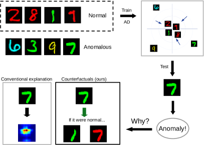
Figure 1: The figure illustrates the benefit of counterfactual explanation of anomaly detectors over traditional methods, using the Colored-MNIST dataset of handwritten digits in various colors. The normal data (top left) consist of digits colored red and instances of the digit one in any color. An example anomaly—a green seven—is shown on the right. Conventional explanation methods localize the anomaly within the image and highlight it on a heatmap (bottom left). Note how the heatmap accentuates the horizontal bar that distinguishes the seven from a one. In contrast, the proposed method transforms the anomaly into multiple counterfactuals, e.g., by erasing the seven’s horizontal bar or altering its color to appear normal. Thus, the proposed counterfactual explanation method addresses the crucial question: “How must the anomaly be altered to appear normal to the detector?"

Anomaly detection is the task of identifying patterns that deviate from normal behavior, the so-called anomalies. These anomalies can correspond to crucial actionable information in various domains such as medicine, manufacturing, surveillance, and environmental monitoring (Chandola et al., 2009; Hartung et al., 2023).

Recently, deep learning-based methods have shown tremendous success in anomaly detection (AD), reducing error rates to approximately $1\%$ in numerous well-established image benchmarks (Reiss et al., 2021; Deecke et al., 2021; Ruff et al., 2021; Liznerski et al., 2022). However, deep learning-based anomaly detectors lack the out-of-the-box interpretability of their traditional counterparts, making it difficult to understand the reasoning behind their predictions (Liznerski et al., 2021). Their lack of transparency is particularly concerning in sectors where safety is crucial and in situations where building trust or preventing social biases are essential (Gupta et al., 2018; Montavon et al., 2018; Samek et al., 2020). Understanding modern anomaly detectors is a major challenge in contemporary AD and a necessary step before using AD in decision-making systems (Ruff et al., 2021).

Although feature-attribution techniques such as anomaly heatmaps (Liznerski et al., 2021; Gudovskiy et al., 2022; Roth et al., 2022) have been explored, they do not explain the underlying semantics of anomalies relevant to the decision-making of the detectors. In domains beyond AD, counterfactual explanation (CE) has emerged as a popular alternative. CE generates synthetic samples that change the model’s prediction with minimal alterations to the original sample (Ghandeharioun et al., 2021; Abid et al., 2022). CEs are user-friendly and can provide explanations on a higher, semantic level, such as illustrated in Figure 1.

In this paper, we propose the use of CE to explain anomaly detectors. To our knowledge, this paper presents the first study of CE in modern image AD based on deep learning. The AD setting comes with several considerable challenges. Anomalies can be rare and unlabeled in AD, making it hard to synthesize realistic counterfactuals based on semantically meaningful concepts that are understandable to humans. Furthermore, normal samples often have limited diversity in AD, which complicates training modern deep generative models.

Contributions

This paper introduces a novel unsupervised method to explain image anomaly detectors using counterfactual examples. While previous approaches identify anomalous regions within images, the presented technique generates a set of counterfactual examples of each anomaly, capturing diverse disentangled aspects (see Figure 1). These counterfactual examples are created by transforming anomalous images into normal ones, guided by a specific aspect. The method provides semantic explanations of anomaly detectors, highlighting the higher-level aspects of an anomaly that triggered the detector. CE allows users to explore “what-if" scenarios (see Figure 1), improving the understanding of the anomaly factors at an unprecedented level of abstraction. Qualitative and quantitative analyses across various well-established image datasets show the effectiveness of the method when applied to state-of-the-art anomaly detectors.

2 Related work

Over the last decade, there has been a significant increase in research on improving the interpretability of non-linear ML methods, particularly neural networks. This surge is driven by the increasingly widespread use of ML in decision-making systems, where the transparency of predictions is imperative and required even by law in many countries (Neuwirth, 2022). In the following, we discuss the research articles that have the greatest relevance to the proposed work. For a general overview of the area of explainable AI, we refer to the survey by Linardatos et al. (2020).

Explanation of image AD

Prior research in explainable image AD has focused predominantly on feature attribution methods, which identify areas in images that influence predictions. Some methods trace an importance score from the model output back to the pixels (Selvaraju et al., 2017; Zhang et al., 2018), others alter parts of the image and measure the impact on the model output. These alterations can include masking and noising (Fong and Vedaldi, 2017), blurring (Fong and Vedaldi, 2017), pixel values (Dhurandhar et al., 2018), or model outputs (Zintgraf et al., 2017). Some of these approaches have been applied to AD (Liznerski et al., 2021; Li et al., 2021; Wang et al., 2021). Several methods generate explanations using generative models or autoencoders, where the pixel-wise reconstruction error yields an anomaly heatmap (Baur et al., 2019; Bergmann et al., 2019; Dehaene et al., 2020; Liu et al., 2020; Venkataramanan et al., 2020). Others use fully convolutional architectures (Liznerski et al., 2021) or transfer learning (Defard et al., 2021; Roth et al., 2022). All these methods visualize the regions within an image that influence the detector’s prediction; however, they do not explain the detectors at a higher semantic level (Alqaraawi et al., 2020; Adebayo et al., 2018).

Counterfactual explanation of neural networks on images

CE methods (Guidotti, 2022) identify the necessary changes in the input to alter the model prediction in a specific way. Unlike feature-attribution techniques, CE methods can explain predictions at a more sophisticated semantic level. These explanations can offer valuable information that improves understanding of model behavior and aligns more closely with human cognition (Pearl, 2009). Existing CE algorithms are designed primarily for supervised learning on tabular data (Wachter et al., 2017; Mothilal et al., 2020; Guidotti, 2022). Some recent studies have also explored the application of CE in image classification (Goyal et al., 2019; Ghandeharioun et al., 2021; Abid et al., 2022; Singla et al., 2023). DISSECT (Ghandeharioun et al., 2021) stands out with its ability to generate multiple CEs with disentangled high-level concepts. However, to date, there is no existing work on the application of CE for image AD.

Counterfactual explanation of AD on shallow data

So far, CE methods for AD have been applied only to “shallow” data types, such as tables (Angiulli et al., 2023; Datta et al., 2022a; Han et al., 2023) or time series (Sulem et al., 2022; Cheng et al., 2022). These methods use knowledge graphs or structural causal models to generate counterfactuals for categorical features (Datta et al., 2022b; Han et al., 2023) or take advantage of temporal aspects (Sulem et al., 2022; Cheng et al., 2022). Some of these methods have been applied to fairness (Han et al., 2023) and algorithmic recourse (Datta et al., 2022a). None of the CE methods for AD are applicable to images, nor are they capable of generating disentangled CEs. This capability is a distinctive feature of the proposed approach, which will be described in the following section.

3 Methodology

In this section, we formally introduce the proposed framework to create counterfactuals for image AD, using state-of-the-art generators. To the best of our knowledge, the approach is the first one to explain image AD using CE.

3.1 Counterfactual Explanations of Image AD

Our aim is to provide explanations for a given anomaly detector $\phi:\mathbb{R}^{D}\rightarrow[0,1]$ that maps an image $x\in\mathbb{R}^{D}$ to an anomaly score $\alpha\in[0,1]$. We define a CE for the detector $\phi$ and anomaly $\bm{x}^{*}\in\mathbb{R}^{D}$ (i.e., $\phi(\bm{x}^{*})\gg 0$) as a sample $\bar{\bm{x}}^{*}$ with $\phi(\bar{\bm{x}}^{*})\approx 0$ and $\lVert\bar{\bm{x}}^{*}-\bm{x}^{*}\rVert_{1}\leq\epsilon$ for an $\epsilon\geq 0$. In other words, a CE has to be normal according to $\phi$ whilst being minimally changed w.r.t. the original anomaly $\bm{x}^{*}$. It thus addresses the question: “What if the anomaly $\bm{x}$ were normal?", thereby explaining the behavior of the anomaly detector at a high semantic level.

To produce such CEs for deep AD, we need to train a generator $G:\mathbb{R}^{D}\rightarrow\mathbb{R}^{D}$ to yield $G(\bm{x}^{*})=\bar{\bm{x}}^{*}$. However, normal images can differ from anomalies in multiple ways, and thus multiple CEs may be required to adequately explain an anomaly. We want the generator to consider multiple concepts $k\in\{1,\dots,K\}$. Thus the generator becomes of the form $G:\mathbb{R}^{D}\times\{1,\dots,K\}\rightarrow\mathbb{R}^{D}$ and is supposed to yield $G(\bm{x}^{*},k)=\bar{\bm{x}}^{*}_{k}$ with $\lVert\bar{\bm{x}}^{*}_{k}-\bar{\bm{x}}^{*}_{k^{\prime}}\rVert_{1}\geq\epsilon^{\prime}$.

The same data $\{(\bm{x}_{0},y_{0}),\dots,(\bm{x}_{n},y_{n})\}$ can be used for training $\phi$ and $G$. Here $y_{i}=0$ denotes normal samples and $y_{i}=1$ anomalies. Note that in the AD setting, the training labels $y_{i}$ are typically unknown and the majority of the samples are assumed to be normal.

3.2 Disentangled Counterfactual Explanations

Outside of the domain of AD, Ghandeharioun et al. (2021) have proposed Disentangled Simultaneous Explanations via Concept Traversal (DISSECT) to create CEs. DISSECT generates sequences of CEs with increasing impact on a classifier’s output. The proposed approach for CE of image anomaly detectors builds on this idea.

We modify the generator $G:\mathbb{R}^{d}\times[0,1]\times\{1,\dots,K\}\rightarrow\mathbb{R}^{D}$ to also consider a target anomaly score $\alpha$ and expect the trained $G$ to yield a sample with anomaly score of approximately $\alpha$. Following DISSECT, we train $G$ as a concept-disentangled GAN (Goodfellow et al., 2020). To this end, we define a discriminator $D:\mathbb{R}^{D}\rightarrow[0,1]$ and a concept classifier $R:\mathbb{R}^{D}\times\mathbb{R}^{D}\rightarrow[0,1]^{K}$. $D$ is trained to distinguish between generated $\bar{\bm{x}}_{\alpha,k}=G(\bm{x},\alpha,k)$ and true samples from the dataset, encouraging realistic outcomes. $R$ classifies the concept $k$ for a sample $\bar{\bm{x}}_{\alpha,k}$, encouraging the generated samples to be concept-disentangled on a semantic level. Further losses encourage the generator to incur minimal changes on the original sample $\bm{x}$ and to yield target anomaly scores $\alpha$ (i.e., $\phi(\bar{\bm{x}}_{\alpha,k})\approx\alpha$).

The proposed method’s objective summarizes to

$$\min_{G,R}\max_{D}\lambda_{gan}\left(L_{D}(D)+L_{G}(G)\right)+\lambda_{\phi}L_{\phi}(G)+$$

$$\lambda_{rec}L_{rec}(G)+\lambda_{rec}L_{cyc}(G)+\lambda_{r}L_{con}(G,R),$$

where $L_{\phi}(G)$ encourages for $\bar{\bm{x}}_{\alpha,k}$ an anomaly score of $\alpha$:

$$L_{\phi}(G)=\alpha\log\big{(}\phi(\bar{\bm{x}}_{\alpha,k})\big{)}+\big{(}1-\alpha\big{)}\log\big{(}1-\phi(\bar{\bm{x}}_{\alpha,k})\big{)}.$$

The losses $L_{D}(D)$ and $L_{G}(G)$ can be any discriminative and generative GAN losses, respectively. Here, we employ a variant with spectral normalization Miyato et al. (2018) and hinge loss Miyato and Koyama (2018):

$$L_{G}(G)=-D(\bar{\bm{x}}_{\alpha,k}),$$

$$L_{D}(D)=-\min(0,-1+D(\bm{x}))-\min(0,-1-D(\bar{\bm{x}}_{\alpha,k})).$$

The reconstruction loss

$$L_{rec}(G)=\left\lVert\bm{x}-G(\bm{x},\phi(\bm{x}),k)\right\rVert_{1}$$

makes $G$ reconstruct $\bm{x}$ for every concept $k$, when conditioned on $\bm{x}$ and its “true” anomaly score $\phi(\bm{x})$. This ensures that $G$ remains unchanged in a sample when the sample already has the targeted anomaly score, overall encouraging minimal changes.

Similarly, the “cycle consistency loss" (Zhu et al., 2017)

$$L_{cyc}(G)=\left\lVert\bm{x}-\tilde{\bm{x}}_{\alpha,k}\right\rVert_{1},$$

where $\tilde{\bm{x}}_{\alpha,k}=G(\bar{\bm{x}}_{\alpha,k},\phi(\bm{x}),k)$, encourages $G$ to recreate the sample $\bm{x}$, when targeting its true anomaly score $\phi(\bm{x})$ and being conditioned on any generated sample $\bar{\bm{x}}_{k,\alpha}$ based on $\bm{x}$. It encourages minimal changes because the generator needs to be able to revert any change of $\bm{x}$.

$L_{con}(G,R)$ compels $G$ to produce disentangled concepts:

$$L_{con}(G,R)=\mathbb{C}\Big{(}k,R\big{(}\bm{x},\bar{\bm{x}}_{\alpha,k}\big{)}\Big{)}+\mathbb{C}\Big{(}k,R\big{(}\bar{\bm{x}}_{k,\alpha},\tilde{\bm{x}}_{\alpha,k}\big{)}\Big{)},$$

where $\mathbb{C}$ denotes the cross entropy loss.

In summary, the losses encourage the generated samples $\bar{\bm{x}}_{\alpha,k}$ to be semantically distinguishable for different concepts $k$ while having an anomaly score of $\alpha$ according to $\phi$ and undergoing minimal changes with respect to  the original $\bm{x}$. This results in a disentangled set of $K$ counterfactual examples for an anomaly $\bm{x}^{*}$ with $\{G(\bm{x}^{*},0,1),\dots,G(\bm{x}^{*},0,K)\}$. Furthermore, the generator can also produce pseudo anomalies $G(\bm{x},\alpha,K)$ when $\phi(\bm{x})\approx 0$ and $\alpha\gg 0$, which can help $G$ learning how to turn anomalies into normal samples, when included in $L_{\phi}$.

3.3 Deep Anomaly Detection

The proposed CE framework is general and can be applied to any anomaly detector that produces real-valued anomaly scores. In this paper, we specifically study three state-of-the-art anomaly detectors that are reviewed below.

DSVDD

One of the first deep approaches to AD is Deep Support Vector Data Description (DSVDD) (Ruff et al., 2018). Similar to many AD methods, DSVDD is unsupervised, employing an unlabeled corpus of data for training. DSVDD trains a neural network $\phi_{\theta}:\mathbb{R}^{D}\rightarrow\mathbb{R}^{d}$ with parameters $\theta$ to map the training data $\bm{x}_{1},\dots,\bm{x}_{n}\in\mathbb{R}^{D}$ into a semantic space $\mathbb{R}^{d}$, where it can be enclosed by a minimal volume hypersphere: $\min_{\theta}\sum_{i=1}^{n}||\phi_{\theta}(\bm{x}_{i})-\bm{c}||^{2}$. In contrast to shallow SVDD (Tax and Duin, 2004), the hypersphere center $\bm{c}\in\mathbb{R}^{d}$ is first randomly initialized and then kept fixed while training. The rationale behind DSVDD is the following. The network is trained to ensure that the normal data clusters tightly within the semantic space. This property might not hold for anomalies, becoming evident through the anomaly’s relatively large distance from the center. This distance is then used as the anomaly score. Since the CE generator requires bounded anomaly scores, we slightly adjust the DSVDD objective to the following:

$$\min_{\theta}\sum_{i=1}^{n}\frac{||\phi_{\theta}(\bm{x}_{i})-\bm{c}||^{2}}{1+||\phi_{\theta}(\bm{x}_{i})-\bm{c}||^{2}}.$$

Outlier Exposure

AD has traditionally been approached as an unsupervised learning problem due to the lack of sufficient training data to characterize the diverse anomaly class, which encompasses everything different from the normal data. However, Hendrycks et al. (2019a) showed that Outlier Exposure (OE)—the approach of using a large unstructured collection of natural images as example anomalies during training—consistently outperforms purely unsupervised AD methods across various image-AD benchmarks. These auxiliary data are called OE samples. It has been found that training a Binary Cross Entropy (BCE) loss to discriminate between the normal data and OE samples performs competitivly for most image-AD tasks. We use the OE samples both for training the detector’s network $\phi$ and the generator $G$. The generator $G$ is thus trained on a more diverse training set that also contains some further examples of presumably anomalous training samples.

Hypersphere Classification

Although OE has proven to be effective in many benchmarks, there are still scenarios where OE samples do not sufficiently represent the anomalies, especially when the normal data are not natural images (Liznerski et al., 2021). To benefit from insufficiently representative training anomalies, the community has further developed semi-supervised AD methods (Görnitz et al., 2014; Ruff et al., 2020). One of the most competitive semi-supervised AD techniques is HyperSphere Classification (HSC) (Liznerski et al., 2022). When combined with OE, the authors observed that this method becomes more robust to the selection of OE data. The HSC loss is a semi-supervised modification of the DSVDD loss:

$$\frac{1}{n}\sum_{i=1}^{n}y_{i}\cdot h\left(\phi_{\theta}(\bm{x}_{i})\right)-(1{-}y_{i})\log{(1{-}\exp{({-}h\left(\phi_{\theta}(\bm{x}_{i})\right))})},$$

where $h$ is the Pseudo-Huber loss $h(\bm{z})=\sqrt{\left\lVert\bm{z}\right\rVert^{2}+1}-1$.

We employ HSC’s original objective but slightly modify the anomaly score from $h\left(\phi_{\theta}(\bm{x}_{i})\right)$ to

$$1-\exp(-h\left(\phi_{\theta}(\bm{x}_{i})\right)),$$

again obtaining bounded anomaly scores for training the proposed counterfactual generator.

4 Experiments

In this section, we empirically assess the capabilities of CEs for deep AD. The evaluation provides qualitative (Section 4.2) and quantitative (Section 4.3) evidence of the superiority of the proposed CEs over their traditional counterparts. Notably, the experiments expose a previously unreported bias of supervised classifiers when used in the AD setting (Section 4.4).

4.1 Experimental Details

We describe the datasets on which we experiment, the experimental setup, and the implementation of the method.

Datasets

We evaluate the proposed approach on the following datasets:

• MNIST (Deng, 2012) is a dataset of grayscale images of handwritten digits with a class for each digit. Following (Liznerski et al., 2021), we use EMNIST (images of handwritten letters) (Cohen et al., 2017) as OE.

• Colored-MNIST, where for each sample in MNIST, copies are created in seven colors (red, yellow, green, cyan, blue, pink, and gray). Analogously, we employ a colored version of EMNIST as OE.

• CIFAR-10 (Krizhevsky et al., 2009) is a dataset of natural images with ten classes, such as cat, ship, or truck. Previous works used 80 Mio. Tiny Images as OE (Hendrycks et al., 2019b). Since this dataset has been withdrawn due to offensive data (Birhane and Prabhu, 2021), we instead use the disjunct CIFAR-100 dataset as OE, which yields approximately the same performance (here 96.0% average AuROC, as reported in Table 9, vs. 96.1% AuROC in Liznerski et al. (2022)).

• GTSDB (Houben et al., 2013) is a dataset of German traffic signs. We use CIFAR-100 as OE.

Experimental Setup

Following previous work on image-AD (Ruff et al., 2018; Golan and El-Yaniv, 2018; Hendrycks et al., 2019a, b; Ruff et al., 2020; Tack et al., 2020; Ruff et al., 2021; Liznerski et al., 2021, 2022), we convert several multi-class classification datasets into AD benchmarks. This is achieved by defining a subset of the classes to be normal and using the remaining classes as ground-truth anomalies during testing. When only one class is considered normal, this approach is known as one vs. rest. In addition to investigating one vs. rest, we also explore a variation in which multiple classes are normal. This setting emulates a multifaceted normal class that includes different notions of normality. Since our method disentangles multiple aspects of the normal data, we hypothesize that it possesses the capability to capture these diverse facets of normality.

For both the MNIST and CIFAR-10 datasets, we construct 30 distinct scenarios: ten scenarios wherein each individual class serves as the normal data, and an additional 20 scenarios featuring various combinations of classes as normal. For the Colored-MNIST dataset, we define seven normal class scenarios through combinations of colors and digits. We consider ten different normal class sets for the GTSDB dataset. For each scenario and several random seeds, we train an AD model and a CE generator. Details of all scenarios are given in Appendix D. Our quantitative analysis reports results averaged over all scenarios and four seeds. Detailed quantitative results for each scenario can be found in Appendix D and a collection of further qualitative results in Appendix E.

Implementation Details

In our experiments, we generate and compare CEs using three state-of-the-art deep AD methods: BCE, HSC, and DSVDD (see Section 3.3). We employ conventional convolutional neural networks with up to five layers for the AD methods. The concept classifier is a small ResNet (He et al., 2016) with two blocks. Both the discriminator and generator are wide ResNets (Zagoruyko and Komodakis, 2016) with four blocks. The $\lambda$ parameters in our loss (Section 3.2) are set to reasonable values that have been found to perform well across all settings. The hyperparameters of the AD methods are chosen as in previous work (Ruff et al., 2018; Liznerski et al., 2022). The epochs and augmentation are slightly reduced for faster training. A description of all hyperparameters and network architectures is given in Appendix C for both the CE generator and AD methods.

4.2 Qualitative Results

In this section, we present qualitative examples of CEs on four datasets, demonstrating the benefit of using CE for AD over traditional explanation methods such as anomaly heatmaps.

4.2.1 Counterfactuals can explain why images are predicted anomalous

Colored-MNIST

Figure 2 shows CEs for Colored-MNIST, when the normal class is formed of instances of the digit one and digits colored cyan.

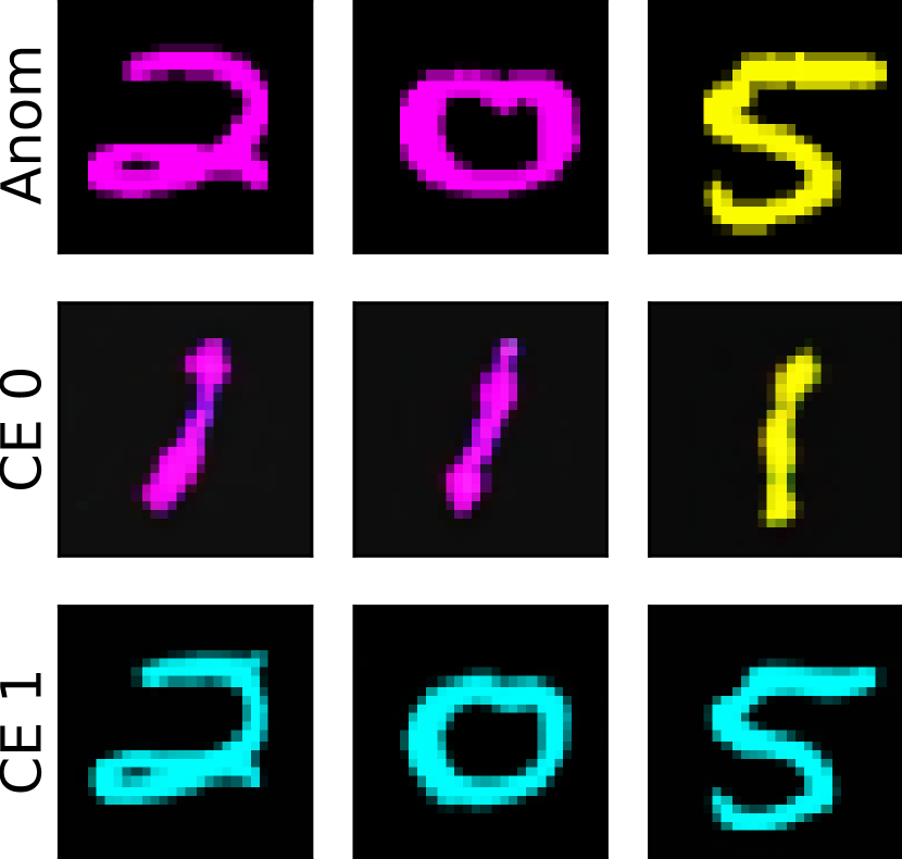
(a) BCE (OE)

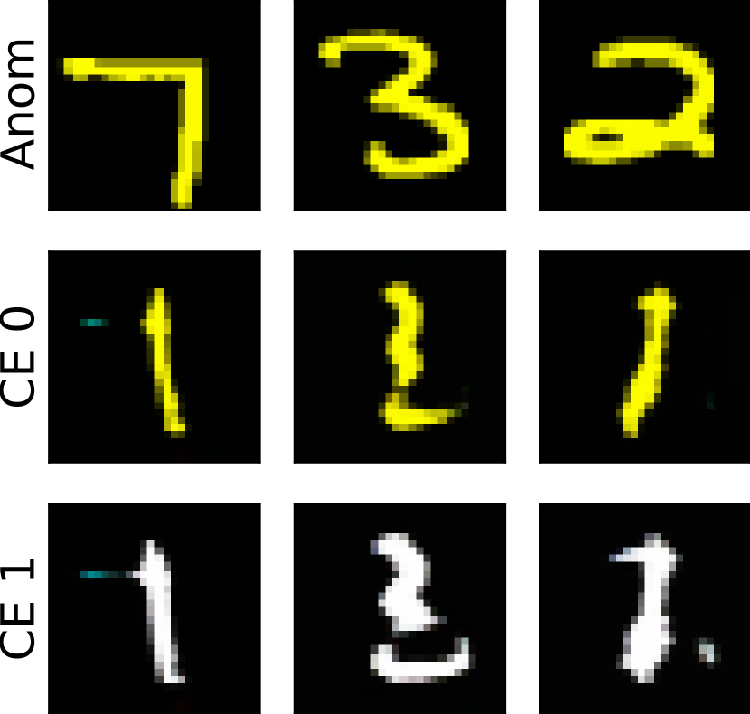
(b) HSC (OE)

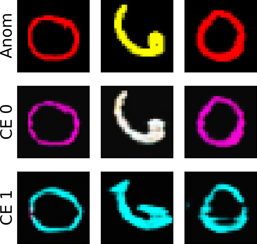
(c) DSVDD

Figure 2: Examples of CEs for the Colored-MNIST dataset, with digits colored cyan and the digit one serving as the normal class. The first row shows the most anomalous images, and the other two rows present CEs derived from these anomalies, using two different concepts. The CEs of BCE and HSC appear normal for each concept.

We observe that the CEs generated to explain the BCE detector align well with our expectation. The proposed method transforms the anomalies into ones without changing the color, or their color is changed to cyan without changing the digit. Both modifications are minimal alterations of the anomaly, transforming its appearance to normality in two distinct ways. The CEs of the HSC method also mostly correspond to normal samples, as expected. However, in some cases both the color and the digit is changed, resulting in unnecessary changes. We found that this behavior represents a local optimum of the objective of our method, highlighting the inherent difficulty of the unsupervised generation of CEs for AD. The CEs created to explain the DSVDD detector perform the least effectively. They tend to appear normal for one concept but often fail for the other concept. This behavior may be attributed to DSVDD’s limited ability to detect anomalies, when compared with the more competitive BCE and HSC detectors, which have the advantage of having access to OE.

MNIST

In Figures 3 and 4, a single digit (seven) or multiple digits (eight and nine) are considered normal, respectively. When the single digit seven is considered normal, the CEs of BCE and HSC are meaningful: the anomalies are transformed into distinct variations of seven. As expected, the CEs of DSVDD are generally of worse quality, sometimes resulting in mere reconstructions of the original anomalous images. Notably, when both the digits eight and nine are considered normal, some anomalies are turned into eights, and others into nines. This observation confirms our hypothesis that the proposed method can correctly reveal diverse notations of normality in multifaceted normal data.

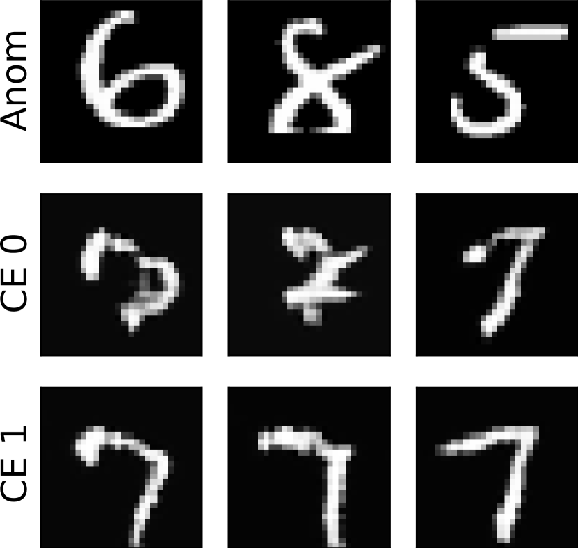
(a) BCE (OE)

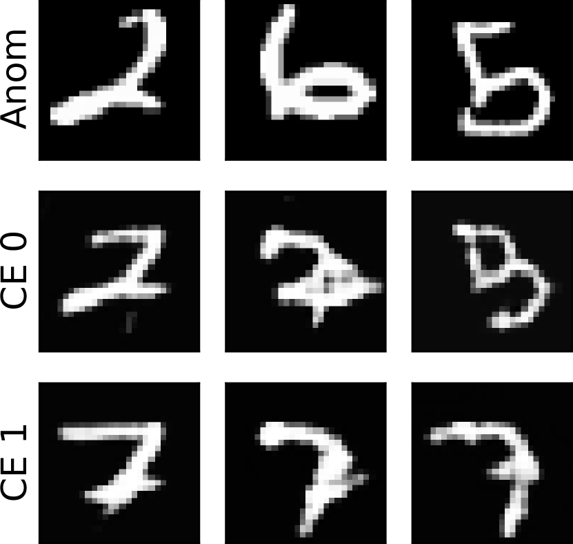
(b) HSC (OE)

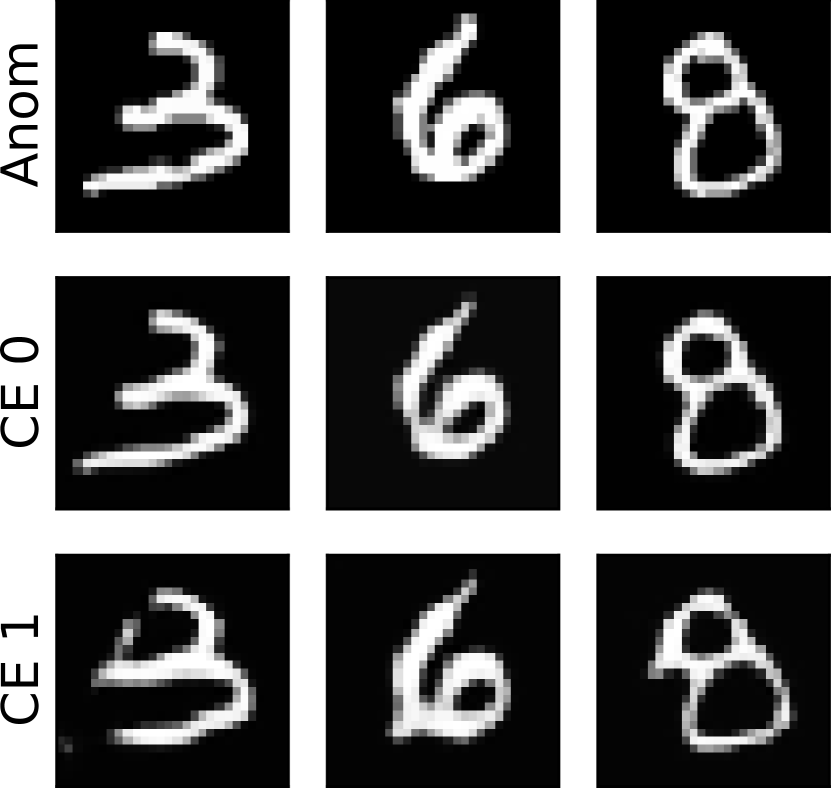
(c) DSVDD

Figure 3: Examples of CEs for MNIST, with the digit seven as the normal class. The first row shows the most anomalous images, the other two rows show CEs using two different concepts. CEs of BCE and HSC are variations of seven and thus represent intuitive counterfactuals.

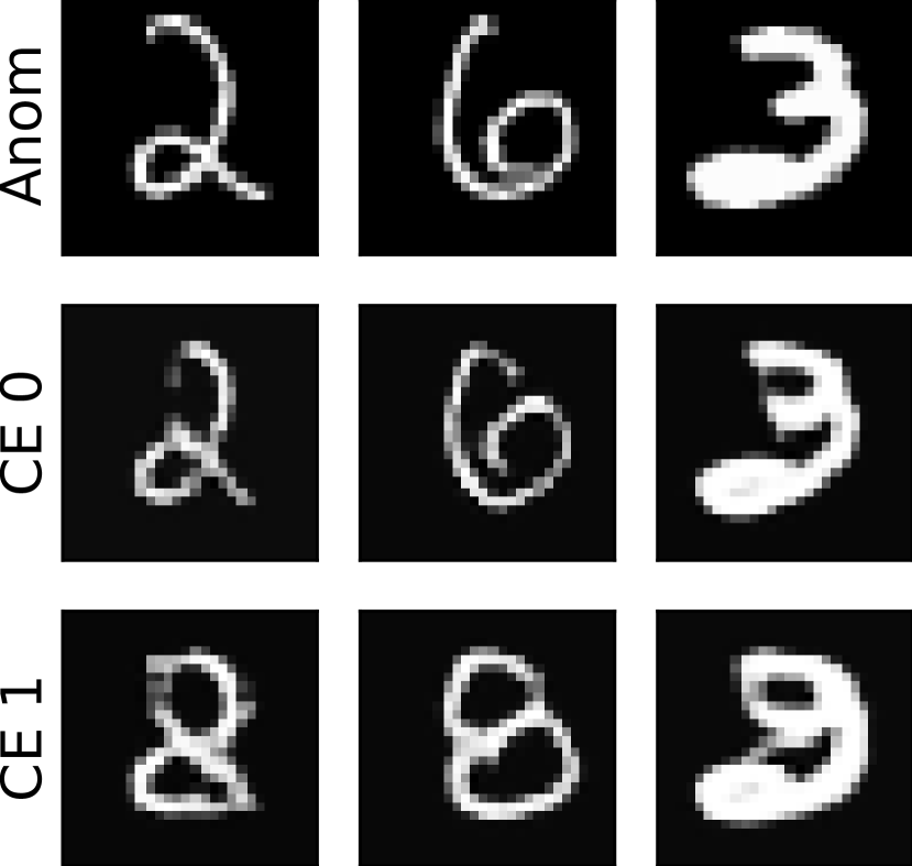
(a) BCE (OE)

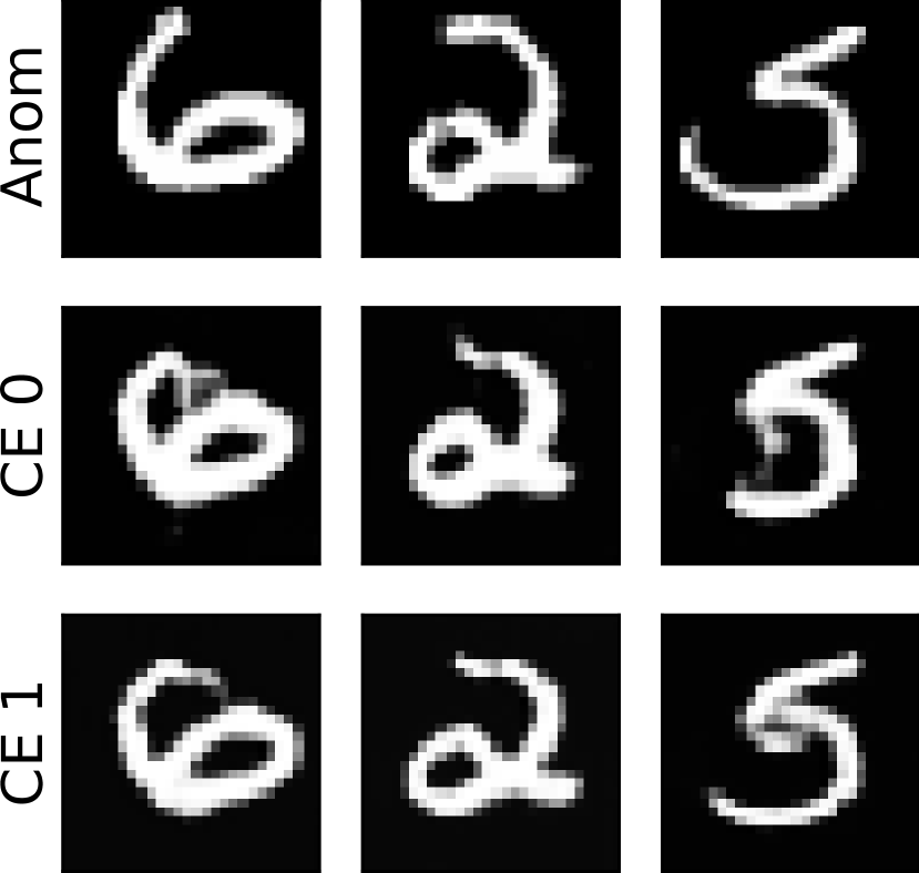
(b) HSC (OE)

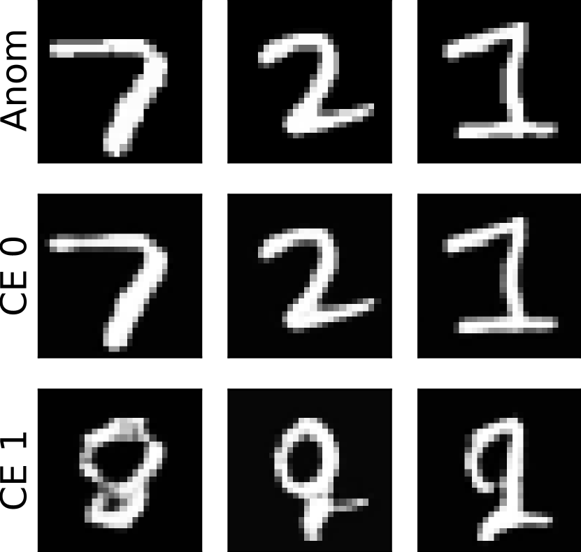
(c) DSVDD

Figure 4: Examples of CEs for MNIST, with digits eight and nine forming the normal class. The first row shows the most anomalous images, the other two rows show CEs using two different concepts. CEs of BCE and DSVDD resemble normal eights or nines for the second concept.

CIFAR-10

Especially for BCE, the CEs for CIFAR-10 in Figure 5 represent intuitive normal samples (ships) that retain the anomalous object’s color to incur minimal changes on the anomaly. The CEs generated for HSC and BCE primarily disentangle the concepts by changing the background. Typically, ships are depicted floating on water, which may vary in color without becoming anomalous. Again, CEs for DSVDD are generally worse, revealing weaknesses of DSVDD as discussed in detail in Appendix A. We refer to Appendix E for more experimental results using other normal classes, showcasing that the CEs exhibit a similar behavior for other classes and combinations of classes forming normality.

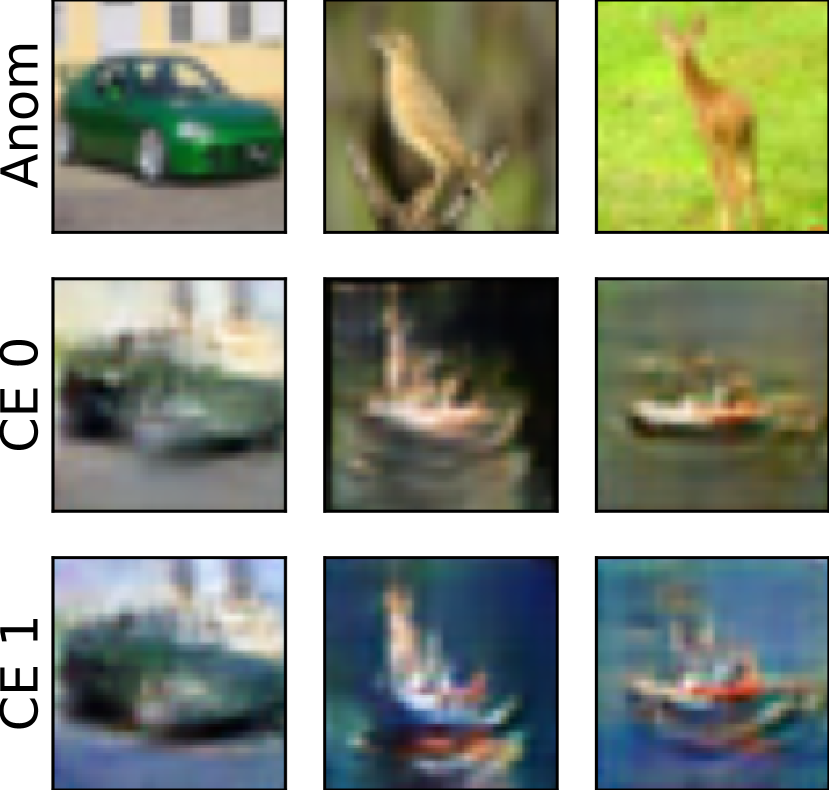
(a) BCE (OE)

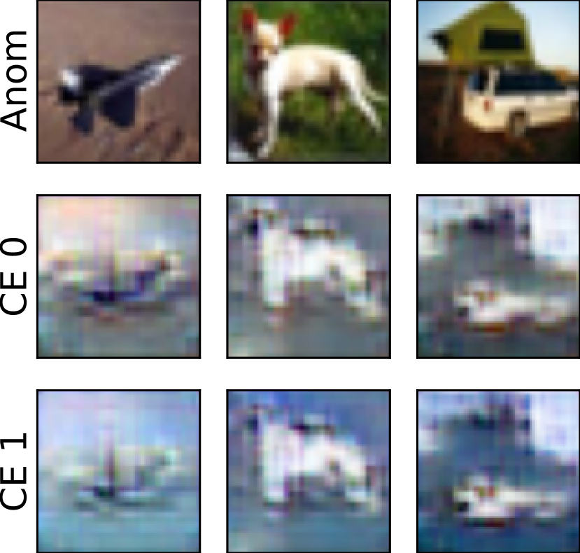
(b) HSC (OE)

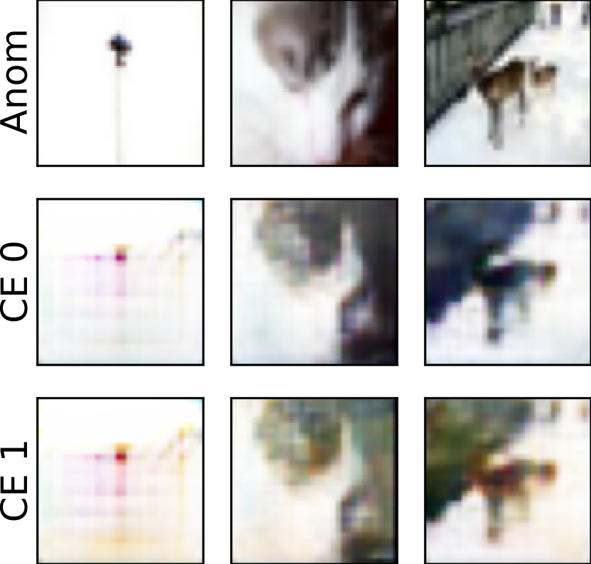
(c) DSVDD

Figure 5: Examples of CEs for CIFAR-10, where images of ships are considered normal. The first row shows the most anomalous images, the other two rows present CEs using two different concepts. The CEs of BCE and HSC display normal ships, varying the background for successful disentanglement while keeping the object’s color to avoid unnecessary changes.

GTSDB

Figure 6 shows the proposed CEs for the GTSDB dataset, when speed signs are taken as a normal class. Again, we refer to Appendix E for more experimental results using other normal scenarios with similar findings. The CEs of BCE and HSC show well-disentangled normal traffic signs, which are obtained from anomalous signs. For instance, the CE of BCE changes the “80km/h restriction ends” sign into a “80km/h limit” sign, which is a minimal intervention to make the sample appear normal.

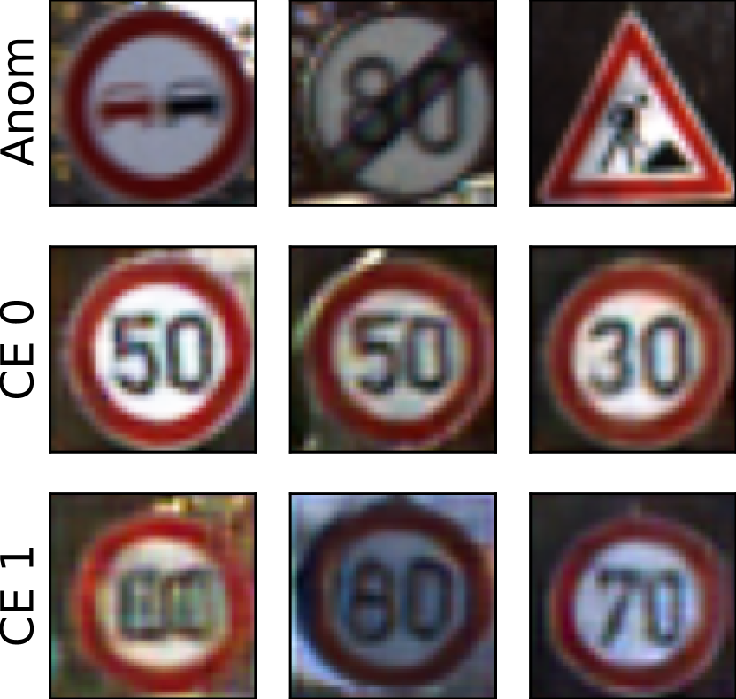
(a) BCE (OE)

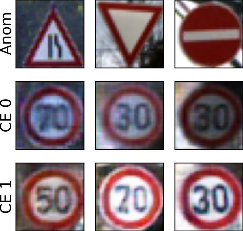
(b) HSC (OE)

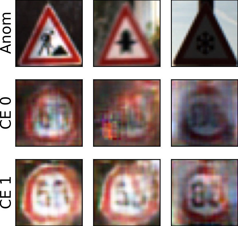
(c) DSVDD

Figure 6: CEs for the GTSDB dataset with images of speed signs forming the normal class. The first row shows the most anomalous images, the other two rows depict CEs corresponding to two different aspects of normality. The CEs of BCE and HSC show well-disentangled normal speed signs with minimal alterations w.r.t. the original anomaly. For instance, the CE transforms the “80km/h restriction ends” into an “80km/h limit” sign.

4.2.2 Counterfactuals can explain why images are predicted anomalous—even when feature attribution fails

In this section, we demonstrate the advantage of the proposed CEs over conventional explanation techniques that attribute features to localize anomalies. Figure 7 (a) shows CEs generated with our method and (b) heatmaps for the corresponding anomalies generated with Fully Convolutional Data Description (FCDD) (Liznerski et al., 2021).

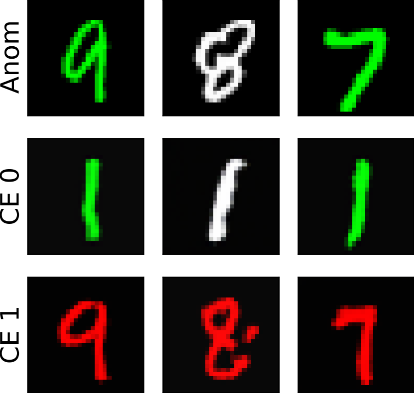
(a) Counterfactuals

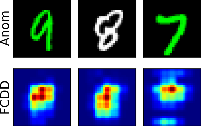
(b) Heatmaps with FCDD

Figure 7: The first row shows anomalies from Colored-MNIST, with red digits and the digit one forming the normal class. The other rows show (a) corresponding CEs for two concepts, and (b) anomaly heatmaps generated with FCDD (Liznerski et al., 2021). The CEs explain the anomaly detector that perceives anomalies turned red or into one as normal, while heatmaps just highlight the difference to one.

FCDD’s heatmaps explain only spatial aspects of the anomalies: FCDD highlights the horizontal bar in digit seven, the circle in digit nine, and almost all of digit eight. These spatial aspects of anomalies are also explained by the CEs created for the first concept, where the anomalies are turned into the digit one. However, FCDD’s heatmaps fail to identify the color as being anomalous, whereas the proposed CEs capture this aspect with their second concept, where the anomalies are colored red, making them appear normal to the detector. This demonstrates that CEs can provide more holistic explanations of anomalies, at a higher semantic level.

4.3 Quantitative Results

This section presents a quantitative analysis of the CEs, assessing their normality, realism, disentanglement, and suitability for training anomaly detectors in terms of various metrics based on AuROC, FID, and accuracy. These metrics are described in detail in Appendix B.

4.3.1 The counterfactuals appear normal

An important attribute for any CE in deep AD is that it must be perceived as normal by the anomaly detector. To evaluate this quality criterion, we compare the anomaly scores of the normal test samples with those of the generated CEs in terms of AuROC. Ideally, the AuROC should approach $50\%$, indicating that CE and normal samples are indistinguishable. As shown in Table 1, the AuROC is indeed very close to $50\%$ on CIFAR-10, GTSDB, and Colored-MNIST (here abbreviated as C-MNIST), underlining that the detector perceives the CEs as normal. Only on MNIST, some of the CEs appear anomalous. This might be due to the enforced disentanglement that produces diverse samples despite of the limited variety of possible normal variations of an anomaly on MNIST.

Table 1: The AuROC of normal test samples vs. CEs. Most of the CEs are perceived as normal with an AuROC close to $50\%$.

Single normal classes Multiple normal classes Method MNIST CIFAR-10 C-MNIST MNIST CIFAR-10 GTSDB BCE OE 72.0 $\pm$ 4.0 47.5 $\pm$ 10.0 55.6 $\pm$ 1.5 78.1 $\pm$ 4.1 49.0 $\pm$ 8.5 50.2 $\pm$ 8.0 HSC OE 80.8 $\pm$ 5.3 49.9 $\pm$ 4.4 55.8 $\pm$ 4.7 82.1 $\pm$ 3.8 44.4 $\pm$ 6.7 48.6 $\pm$ 14.4 DSVDD 75.2 $\pm$ 9.2 54.6 $\pm$ 3.4 61.5 $\pm$ 4.3 73.4 $\pm$ 6.5 50.7 $\pm$ 3.3 53.1 $\pm$ 4.8

4.3.2 The counterfactuals can be used to train an anomaly detector effectively

If the CEs resemble normal images, they will be viable as normal training samples. We retrain the AD methods using CEs in place of the normal training set and report the AuROC for normal vs. anomalous test samples in Table 2.

Table 2: AuROC of normal vs. anomalous test samples when the anomaly detector is trained with the normal training set being substituted with CEs. The results indicate that the CEs are viable normal training samples, as the AuROC values are mostly significantly above the chance level of $50\%$.

Single normal classes Multiple normal classes Method MNIST CIFAR-10 C-MNIST MNIST CIFAR-10 GTSDB BCE OE 91.3 $\pm$ 4.6 59.0 $\pm$ 6.1 80.6 $\pm$ 4.5 62.2 $\pm$ 13.2 58.7 $\pm$ 4.6 90.1 $\pm$ 5.3 HSC OE 85.6 $\pm$ 9.2 54.8 $\pm$ 2.6 81.7 $\pm$ 4.8 54.7 $\pm$ 9.9 53.1 $\pm$ 1.8 89.9 $\pm$ 5.1 DSVDD 46.2 $\pm$ 10.5 50.8 $\pm$ 3.2 59.9 $\pm$ 8.4 41.6 $\pm$ 4.5 49.7 $\pm$ 4.1 58.4 $\pm$ 7.0

The AD methods significantly outperform a random detector when trained with CEs, affirming their viability as normal samples. A notable exception is DSVDD, a method that does not utilize OE and struggles when trained purely with CEs. Table 3 shows the AuROC values when the models are trained with the proper normal training set.

Table 3: AD performance in terms of the AuROC of normal vs. anomalous test samples. BCE and HSC outperform DSVDD and consistently yield error rates of less than $10\%$.

Single normal classes Multiple normal classes Method MNIST CIFAR-10 C-MNIST MNIST CIFAR-10 GTSDB BCE OE 97.7 $\pm$ 1.5 96.0 $\pm$ 2.5 97.1 $\pm$ 1.0 93.5 $\pm$ 2.8 93.8 $\pm$ 2.7 94.3 $\pm$ 4.7 HSC OE 97.6 $\pm$ 1.6 95.9 $\pm$ 2.5 95.7 $\pm$ 2.3 92.9 $\pm$ 3.3 94.0 $\pm$ 2.7 93.0 $\pm$ 5.6 DSVDD 78.8 $\pm$ 8.6 55.4 $\pm$ 4.7 76.9 $\pm$ 6.5 75.4 $\pm$ 7.1 52.6 $\pm$ 3.6 58.2 $\pm$ 6.7

4.3.3 The counterfactuals are realistic

To assess the realism of the CEs, we compute the FID between them and normal test samples. For an intuitive score, we normalize the FID for CEs by dividing through the FID between normal and anomalous test samples. The normalized FID is $100\%$ if the CEs are equally realistic as the anomalies. Details are provided in Appendix B. We found that a normalized FID of $50$ to $100\%$ is a reasonable target for expressive CEs. If the CEs became too similar to the normal data distribution, they would not be valid counterfactuals, as they would not retain non-anomalous features from the anomalies. Table 4 displays the normalized FID scores. The CEs for BCE and HSC are mostly as realistic as the anomalies. On MNIST and Color-MNIST, the CEs are even more realistic than the anomalies. As CEs for DSVDD tend to reconstruct anomalies, their realism is also reasonable.

Table 4: Normalized FID scores for the CEs. Most of the CEs are as realistic as the anomalies, which are also realistic since they follow the general data distribution (e.g., are digits in case of MNIST).

Single normal classes Multiple normal classes Method MNIST CIFAR-10 C-MNIST MNIST CIFAR-10 GTSDB BCE OE 43 $\pm$ 8.1 116 $\pm$ 20.8 56 $\pm$ 12.4 78 $\pm$ 26.0 103 $\pm$ 27.9 110 $\pm$ 101.8 HSC OE 68 $\pm$ 14.6 300 $\pm$ 90.0 95 $\pm$ 30.5 96 $\pm$ 25.0 254 $\pm$ 69.7 95 $\pm$ 73.5 DSVDD 100 $\pm$ 8.8 116 $\pm$ 12.0 83 $\pm$ 8.7 100 $\pm$ 10.7 110 $\pm$ 10.0 131 $\pm$ 118.1

4.3.4 The counterfactuals capture multiple disentangled aspects

Here we show that, for each anomaly, our method generates concept-disentangled CEs. Recall that the concept classifier is trained to predict the concept of each CE (see Section 3). Consequently, we have a metric for assessing the disentanglement of the generated samples. We present the accuracy of this concept classifier in Table 5.

Table 5: The accuracy of the concept classifier for CEs. It is consistently high (except for DSVDD), showing that the CEs are disentangled based on different concepts.

Single normal classes Multiple normal classes Method MNIST CIFAR-10 C-MNIST MNIST CIFAR-10 GTSDB BCE OE 94.3 $\pm$ 3.9 93.0 $\pm$ 4.3 99.4 $\pm$ 1.3 93.8 $\pm$ 5.1 86.2 $\pm$ 7.5 98.8 $\pm$ 0.8 HSC OE 90.8 $\pm$ 4.8 98.8 $\pm$ 3.2 98.9 $\pm$ 2.0 85.7 $\pm$ 9.6 98.9 $\pm$ 2.4 94.0 $\pm$ 8.4 DSVDD 77.5 $\pm$ 14.1 97.1 $\pm$ 2.9 98.0 $\pm$ 3.0 81.6 $\pm$ 11.3 92.2 $\pm$ 4.2 93.4 $\pm$ 4.5

Our models demonstrate a consistent ability to disentangle concepts effectively, with the exception of the results for DSVDD, which has a suboptimal AD performance, making it hard to provide explanations in general. Notably, disentanglement is effective even in the case where just one class is considered normal. On CIFAR-10, the generator exploits the background, whereas on MNIST, it generates disentangled variants of digits. We hypothesize that this strong disentanglement on MNIST is the reason behind the counterfactuals appearing less normal for MNIST.

4.4 Counterfactuals reveal a previously unreported classifier bias in deep AD

In this section, we present a scientific finding: classifiers may be biased when trained for deep AD. Although the hypothesis of “classification bias” has been circulating in the AD literature, suggesting that supervised classifiers may underperform when trained on limited and biased subsets of anomalies (Ruff et al., 2020), this hypothesis has not yet been thoroughly investigated. To examine this hypothesis, we train a supervised classifier on the Colored-MNIST dataset, aiming to distinguish between a normal set (consisting of red digits and the digit one) and a subset of the ground-truth anomalies, specifically all blue ground-truth anomalies. We select a subset of the anomalies for training to simulate a realistic scenario in which one has no access to all variations of the ground-truth anomalies. A key requirement in AD is the model’s ability to identify all forms of unseen anomalies. The classifier bias becomes apparent as the AuROC of normal test samples vs. ground-truth anomalies decreases from $98$ for BCE with OE (unsupervised) to $75$ for supervised BCE. Our CEs further illuminate this phenomenon, as depicted in Figure 8.

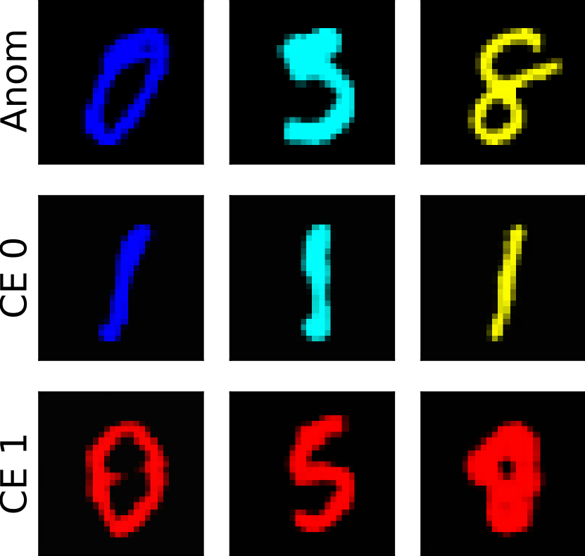
(a) BCE with OE

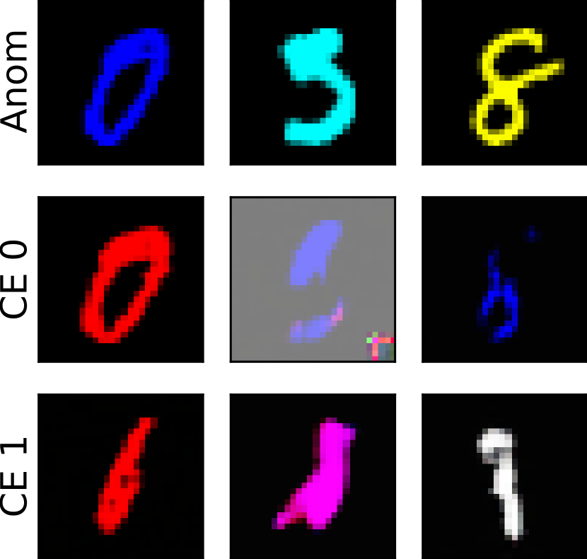
(b) BCE with blue anomalies

Figure 8: The first row shows anomalies for Colored-MNIST with red digits and the digit one forming the normal class. The other two rows present CEs of BCE trained with OE in (a) and of a classifier trained with just blue anomalies in (b). The generator’s inability to generate normal-looking CEs for anomalies other than blue suggests that the classifier in (b) is biased.

While our explanation for the AD method with OE in (a) indicates that anomalies should be transformed into red or digit one to appear normal, they depict a different picture for the supervised classifier in (b). Here, only for the blue anomalous zero, which is seen during training, the CEs roughly show intuitive normal versions of the anomaly. For other unseen anomalies, such as the cyan five or yellow eight, the explanations do not show intuitive normal images. This suggests that the classifier is biased towards detecting blue as anomalous and fails to generalize to other colors not present in the training set. This underlines the need for specialized AD methods (e.g., using OE or semi-supervised objectives) because they are less prone to bias. Our approach is the first to explain such a bias.

5 Conclusion

This paper introduced a novel method that can interpret image anomaly detectors at a semantic level. This is achieved by modifying anomalies until they are perceived as normal by the detector, creating instances known as counterfactuals. Counterfactuals play a crucial role in many scientific disciplines, from causal inference in epidemiology to decision-making in economics and predictive models in climate science. We found that counterfactuals can provide a deeper, more nuanced understanding of image anomaly detectors, far beyond the traditional feature-attribution level. Extensive experiments across various image benchmarks and deep anomaly detectors demonstrated the efficacy of the proposed approach. This research marks a paradigm shift and a significant departure from the more superficial interpretation of anomaly detectors using feature attribution, enhancing our understanding of detectors on a more abstract, semantic level. This may be a substantial milestone in the pursuit of more transparent and accountable AD systems.

Future work could investigate the application of CE to detect subtle defects, known as “low-level anomalies” (Ruff et al., 2021). These anomalies, with their subtle characteristics, present a challenge to explainable AD (Bergmann et al., 2019), and CE promises to enhance our understanding of low-level anomaly detectors. Furthermore, future endeavors could seek to broaden the scope of our work by applying it to diverse data types, such as generating counterfactuals based on latent concepts within tabular data. Current research mainly focuses on altering features to generate counterfactuals, and the proposed method’s exploration of intricate latent factors in the data could greatly improve our understanding in complex data scenarios.

Broader impact

As an explanation technique, our method naturally aids in making deep AD more transparent. It may reveal biases in the model (see Section 4.4) and improve trustworthiness. For example, it may reveal a social bias when a portrait of a person is labeled anomalous due to race or gender. In this scenario, our method might generate CEs where merely the skin color has been changed. Applying our method can prevent a harmful deployment of such an AD model.

Appendix A Limitations of our approach

In the main paper, we proposed a method to generate counterfactual explanations (CEs) for deep anomaly detection (AD). As seen in Section 4, the quality of the generated counterfactual explanations relies on the performance of the AD model. DSVDD without OE (Ruff et al., 2018) performs weakly on some image datasets. Consequently, CEs for DSVDD are often not very intuitive and sometimes collapse to a mere reconstruction of the anomaly. This happens because DSVDD struggles to recognize an anomaly and thus assigns a low anomaly score to it. Our method doesn’t have a reason to change an anomaly to turn it normal for DSVDD. Another limitation of our method is that the generator might change more than necessary to turn the anomaly normal, thereby falling into a local optimum of the overall objective. Learning to balance the objectives of our method in an unsupervised manner is challenging, especially given the limited variety and amount of normal samples. Future work may improve upon this.

Appendix B Metrics

In this section, we provide details on the metrics used for the quantitative analysis in Section 4.3.

Normality of counterfactuals

To assess the normality of the generated CEs, we computed the AuROC of normal test samples against CEs generated for all ground-truth anomalies from the test set. The Area Under the ROC curve (AuROC) is a widely recognized metric in the AD literature for comparing anomaly scores of normal and anomalous samples (Hanley and McNeil, 1982). An AuROC of $1$ indicates perfect separation between anomalies and normal samples, $0.5$ corresponds to random guessing, and a score below $0.5$ suggests anomalies appear more normal than the actual normal samples. To assess the normality of our CEs, we computed the AuROC with the anomalies being CEs. Then, an AuROC of significantly more than $0.5$ indicates that the CEs retain some degree of anomalousness according to the chosen detector. An AuROC of $0.5$ indicates that the CEs appear entirely normal, and for below $0.5$ the CEs are even more normal than the normal test samples. This may happen when the anomaly detector doesn’t generalize perfectly and hence perceives some normal test samples as somewhat anomalous.

Usefulness of counterfactuals for training AD

To further evaluate the normality and realism of the CEs, we tested their ability to train a new anomaly detector. To this end, we replaced the entire normal training set with a collection of CEs generated for all ground-truth anomalies. With this modified training set, we retrained the AD methods, additionally using an outlier exposure set in case of BCE and HSC. If the CEs resemble normal images, the retrained anomaly detectors will outperform random guessing. We measure this by computing the AuROC for true normal vs. anomalous test samples and compare the outcome to the chance level, which is $0.5$.

Realism of counterfactuals

To assess the realism of generated samples, the standard approach involves computing the Fréchet inception distance (FID) introduced by Heusel et al. (2017) for GANs. The FID is the Wasserstein distance between the feature distributions of a generated dataset and a ground-truth dataset. The larger the distance, the less the generated dataset resembles the ground truth. The features are extracted using an InceptionNet v3 model (Szegedy et al., 2015) trained on ImageNet. In this paper, we used the normal test set as ground truth and a collection of CEs for all test anomalies as the generated dataset. For a more intuitive scoring, we also computed a second FID with the test anomalies as the generated dataset. Then, we normalize the FID for CEs by dividing through the FID for test anomalies. The normalized FID is $100\%$ if the CEs are as realistic as the test anomalies, below $100\%$ if they are more realistic, and $0\%$ if they exactly match the normal test set. It is important to note that, although anomalies are naturally anomalous, they are still realistic in the sense that they come from the same classification dataset and thus follow the general distribution of, e.g., handwritten digits. A normalized FID of $100\%$ is therefore sufficient for a counterfactual to be expressive. A normalized FID of close to $0\%$ would actually be spurious, as the generator then seems to entirely reproduce normal samples that don’t retain non-anomalous features from the anomaly.

Disentanglement of counterfactuals

We also evaluated the disentanglement of the sets of CEs for each anomaly. As introduced in Section 3, the proposed method includes a concept classifier trained to predict the concept of each CE. Consequently, we have a metric for assessing the disentanglement of the generated samples. The larger the accuracy of this classifier, the stronger the disentanglement of the generated CEs. We chose a rather small network for the concept classifier to encourage the network no to overfit on non-semantic features to predict the concepts.

Appendix C Hyperparameters

In this section, we provide an exhaustive enumeration of all the hyperparameters that we used for training our AD and CE module. All hyperparameters were adopted from existing research (Ruff et al., 2018; Ghandeharioun et al., 2021; Liznerski et al., 2022). We start by describing the CE module, which is the same for all datasets and AD objectives. Then we separately describe the AD module and other hyperparameters for MNIST, Colored-MNIST, CIFAR-10, and GTSDB.

C.1 The CE Module

Generator

The generator is a wide ResNet (Zagoruyko and Komodakis, 2016) structured as an encoder-decoder network. The encoder consists of a sequential arrangement of a batch normalization layer, a convolutional layer with $64$ kernels, and three residual blocks. Each residual block comprises two sets, each containing a conditional batch normalization layer (De Vries et al., 2017), followed by an activation function (ReLU), and a convolutional layer. The convolutional layers in these sets have $256$, $512$, and $1024$ kernels, respectively, for the first, second, and third block. The initial two residual blocks employ average pooling in each set to reduce the spatial dimension of the feature maps by one-half of the input, while the third residual block is implemented without average pooling to maintain the spatial dimension. Conversely, the decoder follows a similar sequential arrangement, featuring three residual blocks, followed by a batch normalization layer, a final convolutional layer mapping to the image space, and an activation function (ReLU). Again, each residual block comprises two sets, each containing a conditional batch normalization layer, followed by RelU activation, and a convolutional layer. The convolutional layers in these sets have $1024$, $512$, and $256$ kernels, respectively, for the first, second, and third block. The first residual block in the decoder retains the spatial dimension, while the subsequent two residual blocks employ an interpolation layer in each set to upsample the spatial dimension by a multiplicative factor of 2 using nearest-neighbor interpolation. We apply spectral normalization to all layers of the decoder, following (Miyato et al., 2018). The last layer of the decoder uses a tanh activation. The conditional information, i.e., the discretized target anomaly score $\alpha$ and the target concept $k$ are transformed into a single categorical condition and processed through the categorical conditional batch normalization layers.

Discriminator

The discriminator contains four residual blocks arranged sequentially, followed by a final linear layer mapping to a scalar. The first block is implemented with two convolutional layers with $64$ kernels, where the first layer is followed by a ReLU activation and the second layer is followed by an average pooling with a kernel size of $2$. The next two residual blocks consist of two convolutional layers, where each one is preceded by a ReLU activation and then in the end followed by an average pooling layer to reduce the spatial dimension to one-half of the input. The fourth residual block also contains two convolutional layers preceded by a ReLU, but does not use any downsampling. The number of kernels in the convolutional layers from the second to fourth block are $128$, $256$, and $512$, respectively. We apply spectral normalization to all layers.

Concept Classifier

The concept classifier is composed of two sequentially arranged residual blocks, succeeded by a linear layer with two outputs for the classification of two concepts. In the first residual block, three convolutional layers are employed with $64$ kernels each. The initial convolutional layer is succeeded by a ReLU activation, and the last two convolutional layers are followed by average pooling layers, which reduce the spatial dimension by a factor of two. The second residual block consists of two convolutional layers with $128$ kernels, each followed by a ReLU activation, followed by an average pooling with a kernel size of two. We take the sum over the remaining spatial dimension to prepare the output for the final linear layer. Again, we apply spectral normalization to all layers.

Training

We train the generator to generate CEs with two disentangled concepts and a discretized target anomaly score $\alpha\in{0,0.5,1}$. The CE module is trained for $350$ ($2000$ for GTSDB) epochs with a batch size of $64$ normal and, if used, $64$ OE samples. The initial learning rate is set to $2e^{-4}$, with reductions by a multiplicative factor of $0.1$ occurring after $300$ and $325$ epochs. For GTSDB, we instead use an initial learning rate of $1e^{-4}$ and reduce it after $1750$ and $1900$ epochs. We employ the Adam optimizer, with the generator and discriminator optimized every 1 and 5 batches, respectively. The CE objective involves a combination of different losses which are weighted using $\lambda$ hyperparameters. Specifically, we set $\lambda_{gan}=1$, $\lambda_{rec}=100$, $\lambda_{\phi}=1$, and $\lambda_{r}=10$. For GTSDB, we instead set $\lambda_{gan}=5$, $\lambda_{rec}=20$, $\lambda_{\phi}=1$, and $\lambda_{r}=10$.

C.2 AD on MNIST

For MNIST and all following datasets, we trained anomaly detectors with a binary cross entropy (BCE) and hypersphere classification (HSC) loss, both with Outlier Exposure (OE) (Hendrycks et al., 2019a), as well as DSVDD (Ruff et al., 2018) without OE.

We use a LeNet-style neural network comprising layers arranged sequentially with no residual connections. The network contains four convolutional layers and two fully-connected layers. Each convolutional layer is followed by batch normalization, a leaky ReLU activation, and max-pooling. The first fully connected layer is followed by batch normalization and a leaky ReLU activation, while the last layer is only a linear transformation. The number of kernels in the convolutional layers are, from first to last, $4$, $8$, $16$, and $32$. The kernel size is increased from the default of $3$ to $5$ for all of these. The two fully connected layers have $64$ and $32$ units, respectively. For DSVDD we remove bias from the network, following (Ruff et al., 2018), and for BCE we add another linear layer with sigmoid activation.

We used Adam for optimization and balanced every batch to contain 128 normal and 128 OE samples during training. We trained the AD model for $80$ epochs starting with a learning rate of $1e^{-4}$, which we reduced to $1e^{-5}$ after $60$ epochs.

C.3 AD on Colored-MNIST

Based on the MNIST dataset, we created Colored-MNIST where for each sample in MNIST six copies in different colors (red, yellow, green, cyan, blue, pink) are created. We use a colored version of EMNIST as OE. The network for Colored-MNIST is a slight variation of the AD network used on MNIST. We remove the last convolutional layer and change the number of kernels for the convolutional layers to $16$, $32$, and $64$, respectively.

We used Adam for optimization, balanced every batch to contain 128 normal and 128 OE samples during training, and train the AD model for $120$ epochs, starting with a learning rate of $5e^{-5}$, reduced to $5e^{-6}$ after $100$ epochs.

C.4 AD on CIFAR-10

For CIFAR-10, previous work used 80 Mio. Tiny Images as OE (Hendrycks et al., 2019b). However, since 80 Mio. Tiny Images has officially been withdrawn due to offensive data, we instead use the disjunct CIFAR-100 dataset as OE. We found that this does not cause a significant drop of performance. Again, we use a slight variation of the AD network used on MNIST. We remove the last convolutional layer and change the number of kernels for the convolutional layers to $32$, $64$, and $128$, respectively. The fully connected layers have $512$ and $256$ units instead.

We used Adam for optimization and balanced every batch to contain 128 normal and 128 OE samples during training. We trained the AD model for $200$ epochs starting with a learning rate of $1e^{-3}$, which we reduced by a factor of $0.1$ after $100$ and $150$ epochs.

C.5 AD on GTSDB

We use the same setup on GTSDB as on CIFAR-10.

Appendix D Full quantitative results per normal class

In the main paper, we proposed a method to generate counterfactual explanations (CEs) for deep anomaly detection on images. We also presented several objective evaluation techniques to validate their performance on MNIST, Colored-MNIST (C-MNIST), CIFAR-10, and GTSDB across different definitions of normality. Following previous work on semantic image-AD (Ruff et al., 2018; Golan and El-Yaniv, 2018; Hendrycks et al., 2019a, b; Ruff et al., 2020; Tack et al., 2020; Ruff et al., 2021; Liznerski et al., 2021, 2022), we turned classification datasets into AD benchmarks by defining a subset of the classes to be normal and using the remainder as ground-truth anomalies for testing. If just one class is normal, this approach is termed one vs. rest AD. Apart from investigating one vs. rest, we also explored a variation with multiple classes being normal. For our experiments, we considered all classes of MNIST and CIFAR-10 as single normal classes and, to keep the computational load at a reasonable level, a subset of 20 normal class combinations. The class combinations were chosen from $\left\{\left(i,(i+1)\mod 10\right)|i\in\{0,\dots,9\}\right\}\cup\left\{\left(i,(i+2)\mod 10\right)|i\in\{0,\dots,9\}\right\}$. For Colored-MNIST, we considered all combinations of color and the digit one as normal. For GTSDB, we considered the following pairs of street signs as normal: all four combinations of speed limit signs, the “give way” and stop sign, and the “danger” and “construction” warning sign. Additionally, we considered four larger sets of normal classes: all “restriction ends” signs, all speed limit signs, all blue signs, and all warning signs. In total, we consider ten different scenarios of normal definitions for GTSDB. For each scenario on each dataset, a new AD model and counterfactual generator was trained for four random seeds.

Due to space constraints, we reported our quantitative results averaged over all normal definitions in the main paper. Here, we report results averaged over four random seeds separately for each normal definition. We consider the following metrics from the main paper:

• The AD AuROC (Section 4.3.2) is the AuROC of normal vs. anomalous test samples, thereby measuring the AD performance of the AD model. $50\%$ is random, $100\%$ indicates optimal separation.

• The CF AuROC (Section 4.3.1) is the AuROC of normal test samples vs. counterfactuals. The counterfactuals appear entirely normal for an AuROC $\leq 50\%$.

• The Sub. AuROC (Section 4.3.2) is the AuROC of normal vs. anomalous test samples when the AD is trained with counterfactuals in place of the normal training set.

• The $FID_{N}$ (Section 4.3.3) denotes the normalized FID scores. $0\%$ indicates that the counterfactuals follow the same feature distribution as normal samples, $100\%$ as anomalies, which are also realistic, and above $100\%$ indicates less realistic counterfactuals.

• The Concept Acc (Section 4.3.4) is the accuracy of the concept classifier. A $100\%$ accuracy indicates optimal disentanglement of the concepts.

Additionally, we report the “Score distance", which is the L1 distance between the average anomaly score of normal and anomalous test samples. Note that the L1 distance between normal training data and OE samples is usually $1$. Thus, the “Score distance" measures the generalizability of the AD model to ground-truth anomalies in terms of anomaly score calibration.

Tables 6, 7, and 8 show results for MNIST and single normal classes for BCE, HSC, and DSVDD, respectively. In Tables 9, 10, and 11, we instead report results for CIFAR-10 and single normal classes for BCE, HSC, and DSVDD, respectively. Tables 12, 13, and 14 show results for Colored-MNIST (here abbreviated as C-MNIST) for BCE, HSC, and DSVDD, respectively. Tables 15, 16, and 17 show results for GTSDB and combined normal classes for BCE, HSC, and DSVDD, respectively. Tables 18, 19, and 20 show results for MNIST and combined normal classes for BCE, HSC, and DSVDD, respectively. Tables 21, 22, and 23 show results for CIFAR-10 and combined normal classes for BCE, HSC, and DSVDD, respectively.

Table 6: AD and explanation performance averaged over 4 random seeds on MNIST for BCE (OE). Each row shows results for a different normal definition.

	AD		Explanation
Normal	AuROC	Score distance	CF AuROC	Sub. AuROC	FIDN	Concept Acc
zero	0.99 $\pm$ 0.0010	0.78 $\pm$ 0.0079	0.76 $\pm$ 0.0684	0.93 $\pm$ 0.0104	0.42 $\pm$ 0.0366	0.97 $\pm$ 0.0360
one	1.00 $\pm$ 0.0005	0.87 $\pm$ 0.0155	0.66 $\pm$ 0.0977	0.97 $\pm$ 0.0107	0.47 $\pm$ 0.4474	0.99 $\pm$ 0.0082
two	0.97 $\pm$ 0.0083	0.69 $\pm$ 0.0379	0.75 $\pm$ 0.0253	0.85 $\pm$ 0.0183	0.56 $\pm$ 0.0431	0.87 $\pm$ 0.0505
three	0.99 $\pm$ 0.0018	0.67 $\pm$ 0.0286	0.77 $\pm$ 0.0242	0.94 $\pm$ 0.0073	0.33 $\pm$ 0.0392	0.89 $\pm$ 0.0834
four	0.97 $\pm$ 0.0090	0.75 $\pm$ 0.0359	0.70 $\pm$ 0.0787	0.88 $\pm$ 0.0457	0.48 $\pm$ 0.0954	0.91 $\pm$ 0.0563
five	0.97 $\pm$ 0.0058	0.65 $\pm$ 0.0398	0.66 $\pm$ 0.0076	0.84 $\pm$ 0.0184	0.44 $\pm$ 0.0405	0.98 $\pm$ 0.0252
six	1.00 $\pm$ 0.0010	0.90 $\pm$ 0.0106	0.71 $\pm$ 0.0527	0.98 $\pm$ 0.0066	0.33 $\pm$ 0.0348	0.96 $\pm$ 0.0359
seven	0.96 $\pm$ 0.0107	0.71 $\pm$ 0.0275	0.70 $\pm$ 0.0519	0.92 $\pm$ 0.0133	0.50 $\pm$ 0.0464	0.96 $\pm$ 0.0281
eight	0.95 $\pm$ 0.0102	0.54 $\pm$ 0.0337	0.72 $\pm$ 0.0817	0.87 $\pm$ 0.0054	0.31 $\pm$ 0.0271	0.94 $\pm$ 0.0794
nine	0.96 $\pm$ 0.0092	0.60 $\pm$ 0.0329	0.77 $\pm$ 0.0147	0.94 $\pm$ 0.0080	0.47 $\pm$ 0.0593	0.97 $\pm$ 0.0189
mean	0.98 $\pm$ 0.0154	0.72 $\pm$ 0.1067	0.72 $\pm$ 0.0400	0.91 $\pm$ 0.0456	0.43 $\pm$ 0.0808	0.94 $\pm$ 0.0385

Table 7: AD and explanation performance averaged over 4 random seeds on MNIST for HSC (OE). Each row shows results for a different normal definition.

	AD		Explanation
Normal	AuROC	Score distance	CF AuROC	Sub. AuROC	FIDN	Concept Acc
zero	0.99 $\pm$ 0.0011	0.81 $\pm$ 0.0306	0.84 $\pm$ 0.0772	0.91 $\pm$ 0.0101	0.58 $\pm$ 0.1412	0.98 $\pm$ 0.0106
one	1.00 $\pm$ 0.0011	0.89 $\pm$ 0.0231	0.88 $\pm$ 0.0783	0.95 $\pm$ 0.0089	0.60 $\pm$ 0.3820	0.90 $\pm$ 0.0868
two	0.98 $\pm$ 0.0013	0.72 $\pm$ 0.0338	0.77 $\pm$ 0.0332	0.77 $\pm$ 0.0438	0.80 $\pm$ 0.3295	0.92 $\pm$ 0.0575
three	0.98 $\pm$ 0.0056	0.67 $\pm$ 0.0166	0.82 $\pm$ 0.0717	0.85 $\pm$ 0.0209	0.48 $\pm$ 0.2057	0.83 $\pm$ 0.1941
four	0.96 $\pm$ 0.0038	0.73 $\pm$ 0.0269	0.80 $\pm$ 0.0658	0.84 $\pm$ 0.0394	0.83 $\pm$ 0.2911	0.81 $\pm$ 0.1526
five	0.96 $\pm$ 0.0054	0.62 $\pm$ 0.0334	0.83 $\pm$ 0.0603	0.70 $\pm$ 0.1316	0.77 $\pm$ 0.1088	0.92 $\pm$ 0.1010
six	1.00 $\pm$ 0.0010	0.88 $\pm$ 0.0211	0.77 $\pm$ 0.0607	0.98 $\pm$ 0.0076	0.84 $\pm$ 0.3493	0.95 $\pm$ 0.0547
seven	0.97 $\pm$ 0.0052	0.71 $\pm$ 0.0066	0.70 $\pm$ 0.0319	0.92 $\pm$ 0.0112	0.52 $\pm$ 0.0301	0.91 $\pm$ 0.0675
eight	0.95 $\pm$ 0.0069	0.52 $\pm$ 0.0334	0.89 $\pm$ 0.0278	0.73 $\pm$ 0.0590	0.88 $\pm$ 0.3052	0.94 $\pm$ 0.0739
nine	0.97 $\pm$ 0.0043	0.59 $\pm$ 0.0192	0.80 $\pm$ 0.0227	0.92 $\pm$ 0.0031	0.53 $\pm$ 0.0739	0.91 $\pm$ 0.0512
mean	0.98 $\pm$ 0.0157	0.72 $\pm$ 0.1156	0.81 $\pm$ 0.0526	0.86 $\pm$ 0.0919	0.68 $\pm$ 0.1464	0.91 $\pm$ 0.0478

Table 8: AD and explanation performance averaged over 4 random seeds on MNIST for DSVDD. Each row shows results for a different normal definition.

	AD		Explanation
Normal	AuROC	Score distance	CF AuROC	Sub. AuROC	FIDN	Concept Acc
zero	0.82 $\pm$ 0.0685	0.01 $\pm$ 0.0038	0.76 $\pm$ 0.0870	0.41 $\pm$ 0.0680	1.16 $\pm$ 0.5100	0.96 $\pm$ 0.0467
one	1.00 $\pm$ 0.0020	0.05 $\pm$ 0.0086	0.99 $\pm$ 0.0054	0.76 $\pm$ 0.1219	1.02 $\pm$ 0.0600	0.84 $\pm$ 0.1254
two	0.72 $\pm$ 0.1254	0.01 $\pm$ 0.0057	0.69 $\pm$ 0.1664	0.34 $\pm$ 0.0203	0.89 $\pm$ 0.0117	0.49 $\pm$ 0.1150
three	0.72 $\pm$ 0.0274	0.00 $\pm$ 0.0036	0.70 $\pm$ 0.0545	0.42 $\pm$ 0.0527	0.90 $\pm$ 0.0234	0.59 $\pm$ 0.1276
four	0.72 $\pm$ 0.0517	0.01 $\pm$ 0.0040	0.65 $\pm$ 0.0669	0.46 $\pm$ 0.0180	0.88 $\pm$ 0.1156	0.80 $\pm$ 0.1840
five	0.73 $\pm$ 0.0316	0.01 $\pm$ 0.0050	0.71 $\pm$ 0.0562	0.44 $\pm$ 0.0632	0.97 $\pm$ 0.0869	0.87 $\pm$ 0.1221
six	0.83 $\pm$ 0.0964	0.01 $\pm$ 0.0126	0.80 $\pm$ 0.1238	0.44 $\pm$ 0.0466	1.08 $\pm$ 0.0339	0.84 $\pm$ 0.1877
seven	0.84 $\pm$ 0.0450	0.01 $\pm$ 0.0135	0.80 $\pm$ 0.0533	0.46 $\pm$ 0.0858	1.04 $\pm$ 0.0408	0.88 $\pm$ 0.0291
eight	0.70 $\pm$ 0.0359	0.00 $\pm$ 0.0007	0.69 $\pm$ 0.0440	0.46 $\pm$ 0.0792	0.99 $\pm$ 0.0775	0.82 $\pm$ 0.0962
nine	0.81 $\pm$ 0.0331	0.01 $\pm$ 0.0056	0.74 $\pm$ 0.0568	0.44 $\pm$ 0.0599	1.09 $\pm$ 0.0822	0.65 $\pm$ 0.3127
mean	0.79 $\pm$ 0.0865	0.01 $\pm$ 0.0119	0.75 $\pm$ 0.0916	0.46 $\pm$ 0.1050	1.00 $\pm$ 0.0876	0.78 $\pm$ 0.1410

Table 9: AD and explanation performance averaged over 4 random seeds on CIFAR-10 for BCE OE. Each row shows results for a different normal definition.

	AD		Explanation
Normal	AuROC	Score distance	CF AuROC	Sub. AuROC	FIDN	Concept Acc
airplane	0.96 $\pm$ 0.0009	0.78 $\pm$ 0.0083	0.47 $\pm$ 0.0372	0.65 $\pm$ 0.0322	1.48 $\pm$ 0.1439	0.93 $\pm$ 0.0659
automobile	0.99 $\pm$ 0.0005	0.87 $\pm$ 0.0026	0.62 $\pm$ 0.0540	0.62 $\pm$ 0.0347	1.08 $\pm$ 0.0582	0.92 $\pm$ 0.0757
bird	0.93 $\pm$ 0.0030	0.65 $\pm$ 0.0020	0.42 $\pm$ 0.0378	0.53 $\pm$ 0.0138	1.42 $\pm$ 0.0777	0.99 $\pm$ 0.0069
cat	0.91 $\pm$ 0.0035	0.55 $\pm$ 0.0127	0.30 $\pm$ 0.0054	0.53 $\pm$ 0.0159	1.37 $\pm$ 0.0773	0.91 $\pm$ 0.1449
deer	0.96 $\pm$ 0.0020	0.74 $\pm$ 0.0043	0.40 $\pm$ 0.0209	0.53 $\pm$ 0.0103	1.09 $\pm$ 0.1095	0.99 $\pm$ 0.0151
dog	0.94 $\pm$ 0.0013	0.64 $\pm$ 0.0051	0.36 $\pm$ 0.0061	0.57 $\pm$ 0.0134	1.23 $\pm$ 0.0777	0.93 $\pm$ 0.1008
frog	0.98 $\pm$ 0.0011	0.79 $\pm$ 0.0067	0.50 $\pm$ 0.0247	0.54 $\pm$ 0.0127	0.80 $\pm$ 0.0652	0.88 $\pm$ 0.1341
horse	0.98 $\pm$ 0.0006	0.82 $\pm$ 0.0060	0.59 $\pm$ 0.0303	0.64 $\pm$ 0.0213	1.21 $\pm$ 0.1013	0.99 $\pm$ 0.0107
ship	0.98 $\pm$ 0.0002	0.85 $\pm$ 0.0032	0.55 $\pm$ 0.0098	0.72 $\pm$ 0.0300	0.93 $\pm$ 0.0810	0.89 $\pm$ 0.0760
truck	0.97 $\pm$ 0.0018	0.78 $\pm$ 0.0080	0.54 $\pm$ 0.0602	0.56 $\pm$ 0.0242	1.03 $\pm$ 0.1231	0.88 $\pm$ 0.2031
mean	0.96 $\pm$ 0.0252	0.75 $\pm$ 0.0964	0.47 $\pm$ 0.1000	0.59 $\pm$ 0.0610	1.16 $\pm$ 0.2078	0.93 $\pm$ 0.0429

Table 10: AD and explanation performance averaged over 4 random seeds on CIFAR-10 for HSC OE. Each row shows results for a different normal definition.

	AD		Explanation
Normal	AuROC	Score distance	CF AuROC	Sub. AuROC	FIDN	Concept Acc
airplane	0.96 $\pm$ 0.0012	0.75 $\pm$ 0.0056	0.51 $\pm$ 0.0754	0.52 $\pm$ 0.0111	2.95 $\pm$ 0.1509	0.89 $\pm$ 0.0873
automobile	0.99 $\pm$ 0.0005	0.85 $\pm$ 0.0030	0.58 $\pm$ 0.0152	0.59 $\pm$ 0.0129	1.71 $\pm$ 0.1914	0.99 $\pm$ 0.0054
bird	0.93 $\pm$ 0.0015	0.62 $\pm$ 0.0018	0.46 $\pm$ 0.0293	0.52 $\pm$ 0.0149	4.81 $\pm$ 0.2365	1.00 $\pm$ 0.0007
cat	0.90 $\pm$ 0.0020	0.53 $\pm$ 0.0072	0.43 $\pm$ 0.0255	0.52 $\pm$ 0.0088	3.98 $\pm$ 0.4753	1.00 $\pm$ 0.0009
deer	0.96 $\pm$ 0.0007	0.71 $\pm$ 0.0040	0.51 $\pm$ 0.0121	0.57 $\pm$ 0.0230	3.45 $\pm$ 0.3143	1.00 $\pm$ 0.0000
dog	0.95 $\pm$ 0.0012	0.65 $\pm$ 0.0047	0.46 $\pm$ 0.0317	0.53 $\pm$ 0.0257	3.09 $\pm$ 0.2897	1.00 $\pm$ 0.0023
frog	0.98 $\pm$ 0.0004	0.77 $\pm$ 0.0043	0.52 $\pm$ 0.0062	0.57 $\pm$ 0.0569	2.92 $\pm$ 0.4138	1.00 $\pm$ 0.0009
horse	0.98 $\pm$ 0.0008	0.79 $\pm$ 0.0040	0.54 $\pm$ 0.0466	0.54 $\pm$ 0.0281	3.13 $\pm$ 0.0463	1.00 $\pm$ 0.0001
ship	0.98 $\pm$ 0.0003	0.83 $\pm$ 0.0027	0.48 $\pm$ 0.0257	0.56 $\pm$ 0.0316	1.86 $\pm$ 0.5187	1.00 $\pm$ 0.0032
truck	0.97 $\pm$ 0.0011	0.77 $\pm$ 0.0055	0.51 $\pm$ 0.0257	0.57 $\pm$ 0.0623	2.19 $\pm$ 0.1318	1.00 $\pm$ 0.0010
mean	0.96 $\pm$ 0.0254	0.73 $\pm$ 0.0939	0.50 $\pm$ 0.0438	0.55 $\pm$ 0.0259	3.01 $\pm$ 0.8998	0.99 $\pm$ 0.0325

Table 11: AD and explanation performance averaged over 4 random seeds on CIFAR-10 for DSVDD. Each row shows results for a different normal definition.

	AD		Explanation
Normal	AuROC	Score distance	CF AuROC	Sub. AuROC	FIDN	Concept Acc
airplane	0.48 $\pm$ 0.0952	-0.00 $\pm$ 0.0022	0.54 $\pm$ 0.0733	0.45 $\pm$ 0.0265	1.28 $\pm$ 0.0382	0.98 $\pm$ 0.0114
automobile	0.51 $\pm$ 0.0339	0.00 $\pm$ 0.0003	0.52 $\pm$ 0.0606	0.49 $\pm$ 0.0198	1.15 $\pm$ 0.0266	0.99 $\pm$ 0.0076
bird	0.54 $\pm$ 0.0375	0.00 $\pm$ 0.0005	0.52 $\pm$ 0.0601	0.51 $\pm$ 0.0133	1.23 $\pm$ 0.0548	0.91 $\pm$ 0.1548
cat	0.52 $\pm$ 0.0216	0.00 $\pm$ 0.0008	0.51 $\pm$ 0.0513	0.50 $\pm$ 0.0260	1.38 $\pm$ 0.1380	0.98 $\pm$ 0.0221
deer	0.65 $\pm$ 0.0312	0.01 $\pm$ 0.0030	0.62 $\pm$ 0.0996	0.53 $\pm$ 0.0611	1.12 $\pm$ 0.0467	1.00 $\pm$ 0.0028
dog	0.53 $\pm$ 0.0259	0.00 $\pm$ 0.0030	0.51 $\pm$ 0.0296	0.50 $\pm$ 0.0195	1.21 $\pm$ 0.0830	0.96 $\pm$ 0.0523
frog	0.60 $\pm$ 0.0692	0.01 $\pm$ 0.0027	0.54 $\pm$ 0.0371	0.57 $\pm$ 0.0747	0.99 $\pm$ 0.0550	0.99 $\pm$ 0.0074
horse	0.56 $\pm$ 0.0253	0.00 $\pm$ 0.0025	0.53 $\pm$ 0.0281	0.51 $\pm$ 0.0143	1.21 $\pm$ 0.0094	1.00 $\pm$ 0.0037
ship	0.57 $\pm$ 0.0543	0.00 $\pm$ 0.0010	0.58 $\pm$ 0.0350	0.53 $\pm$ 0.0561	0.97 $\pm$ 0.0611	0.93 $\pm$ 0.0758
truck	0.58 $\pm$ 0.0673	0.00 $\pm$ 0.0008	0.58 $\pm$ 0.0470	0.48 $\pm$ 0.0224	1.10 $\pm$ 0.0258	0.97 $\pm$ 0.0417
mean	0.55 $\pm$ 0.0473	0.00 $\pm$ 0.0022	0.55 $\pm$ 0.0336	0.51 $\pm$ 0.0315	1.16 $\pm$ 0.1195	0.97 $\pm$ 0.0287

Table 12: AD and explanation performance averaged over 4 random seeds on C-MNIST for BCE (OE). Each row shows results for a different normal definition.

	AD		Explanation
Normal	AuROC	Score distance	CF AuROC	Sub. AuROC	FIDN	Concept Acc
gray+one	0.96 $\pm$ 0.0037	0.17 $\pm$ 0.0127	0.55 $\pm$ 0.1105	0.75 $\pm$ 0.0429	0.75 $\pm$ 0.3352	0.96 $\pm$ 0.0327
yellow+one	0.97 $\pm$ 0.0027	0.24 $\pm$ 0.0129	0.56 $\pm$ 0.0252	0.74 $\pm$ 0.0082	0.60 $\pm$ 0.1572	1.00 $\pm$ 0.0001
cyan+one	0.96 $\pm$ 0.0138	0.19 $\pm$ 0.0373	0.54 $\pm$ 0.0410	0.83 $\pm$ 0.0180	0.38 $\pm$ 0.0340	1.00 $\pm$ 0.0007
green+one	0.99 $\pm$ 0.0044	0.49 $\pm$ 0.0546	0.58 $\pm$ 0.0457	0.80 $\pm$ 0.0676	0.60 $\pm$ 0.2606	1.00 $\pm$ 0.0001
blue+one	0.98 $\pm$ 0.0034	0.48 $\pm$ 0.0110	0.55 $\pm$ 0.0075	0.81 $\pm$ 0.0640	0.52 $\pm$ 0.1925	1.00 $\pm$ 0.0002
pink+one	0.97 $\pm$ 0.0021	0.25 $\pm$ 0.0193	0.57 $\pm$ 0.0279	0.88 $\pm$ 0.0127	0.43 $\pm$ 0.0647	1.00 $\pm$ 0.0003
red+one	0.98 $\pm$ 0.0031	0.42 $\pm$ 0.0364	0.54 $\pm$ 0.1100	0.83 $\pm$ 0.0938	0.69 $\pm$ 0.4817	1.00 $\pm$ 0.0015
mean	0.97 $\pm$ 0.0101	0.32 $\pm$ 0.1265	0.56 $\pm$ 0.0154	0.81 $\pm$ 0.0451	0.57 $\pm$ 0.1240	0.99 $\pm$ 0.0132

Table 13: AD and explanation performance averaged over 4 random seeds on C-MNIST for HSC (OE). Each row shows results for a different normal definition.

	AD		Explanation
Normal	AuROC	Score distance	CF AuROC	Sub. AuROC	FIDN	Concept Acc
gray+one	0.92 $\pm$ 0.0075	0.27 $\pm$ 0.0410	0.51 $\pm$ 0.0486	0.76 $\pm$ 0.0457	0.86 $\pm$ 0.1567	0.99 $\pm$ 0.0136
yellow+one	0.94 $\pm$ 0.0251	0.43 $\pm$ 0.0509	0.54 $\pm$ 0.0615	0.82 $\pm$ 0.0081	0.82 $\pm$ 0.2713	1.00 $\pm$ 0.0020
cyan+one	0.97 $\pm$ 0.0196	0.39 $\pm$ 0.0630	0.56 $\pm$ 0.0296	0.88 $\pm$ 0.0462	0.63 $\pm$ 0.2201	1.00 $\pm$ 0.0000
green+one	0.98 $\pm$ 0.0139	0.52 $\pm$ 0.0258	0.56 $\pm$ 0.0323	0.89 $\pm$ 0.0102	0.94 $\pm$ 0.2280	1.00 $\pm$ 0.0005
blue+one	0.99 $\pm$ 0.0028	0.65 $\pm$ 0.0159	0.66 $\pm$ 0.0896	0.75 $\pm$ 0.1384	1.66 $\pm$ 1.1219	0.94 $\pm$ 0.0834
pink+one	0.94 $\pm$ 0.0139	0.38 $\pm$ 0.0323	0.52 $\pm$ 0.0751	0.83 $\pm$ 0.0339	0.83 $\pm$ 0.0292	1.00 $\pm$ 0.0015
red+one	0.98 $\pm$ 0.0031	0.60 $\pm$ 0.0127	0.57 $\pm$ 0.0244	0.78 $\pm$ 0.0674	0.93 $\pm$ 0.3331	1.00 $\pm$ 0.0055
mean	0.96 $\pm$ 0.0231	0.46 $\pm$ 0.1226	0.56 $\pm$ 0.0472	0.82 $\pm$ 0.0482	0.95 $\pm$ 0.3047	0.99 $\pm$ 0.0198

Table 14: AD and explanation performance averaged over 4 random seeds on C-MNIST for DSVDD. Each row shows results for a different normal definition.

	AD		Explanation
Normal	AuROC	Score distance	CF AuROC	Sub. AuROC	FIDN	Concept Acc
gray+one	0.73 $\pm$ 0.0350	0.00 $\pm$ 0.0001	0.56 $\pm$ 0.0449	0.71 $\pm$ 0.0755	0.85 $\pm$ 0.2079	0.91 $\pm$ 0.0834
yellow+one	0.86 $\pm$ 0.0262	0.00 $\pm$ 0.0010	0.60 $\pm$ 0.0595	0.65 $\pm$ 0.0639	0.82 $\pm$ 0.2240	1.00 $\pm$ 0.0044
cyan+one	0.83 $\pm$ 0.0866	0.00 $\pm$ 0.0005	0.61 $\pm$ 0.0781	0.63 $\pm$ 0.0589	0.79 $\pm$ 0.0524	0.99 $\pm$ 0.0057
green+one	0.64 $\pm$ 0.1336	0.00 $\pm$ 0.0003	0.57 $\pm$ 0.0250	0.60 $\pm$ 0.0755	0.69 $\pm$ 0.0350	1.00 $\pm$ 0.0019
blue+one	0.78 $\pm$ 0.1502	0.00 $\pm$ 0.0001	0.68 $\pm$ 0.2173	0.42 $\pm$ 0.1223	1.01 $\pm$ 0.1866	1.00 $\pm$ 0.0016
pink+one	0.75 $\pm$ 0.1343	0.00 $\pm$ 0.0001	0.67 $\pm$ 0.1040	0.61 $\pm$ 0.0999	0.85 $\pm$ 0.0998	0.97 $\pm$ 0.0214
red+one	0.79 $\pm$ 0.0424	0.00 $\pm$ 0.0004	0.62 $\pm$ 0.0917	0.57 $\pm$ 0.1607	0.81 $\pm$ 0.1763	0.99 $\pm$ 0.0149
mean	0.77 $\pm$ 0.0650	0.00 $\pm$ 0.0003	0.61 $\pm$ 0.0430	0.60 $\pm$ 0.0841	0.83 $\pm$ 0.0875	0.98 $\pm$ 0.0297

Table 15: AD and explanation performance averaged over 4 random seeds on GTSDB for BCE OE. Each row shows results for a different normal definition.

AD Explanation Normal AuROC Score distance CF AuROC Sub. AuROC FID_N Concept Acc speed limit 30 + 50 0.92 $\pm$ 0.0037 0.65 $\pm$ 0.0103 0.51 $\pm$ 0.0563 0.88 $\pm$ 0.0158 0.77 $\pm$ 0.3590 1.00 $\pm$ 0.0018 speed limit 50 + 70 0.88 $\pm$ 0.0151 0.59 $\pm$ 0.0188 0.49 $\pm$ 0.0576 0.86 $\pm$ 0.0066 0.69 $\pm$ 0.3249 0.99 $\pm$ 0.0080 speed limit 70 + 100 0.88 $\pm$ 0.0053 0.57 $\pm$ 0.0048 0.55 $\pm$ 0.0708 0.89 $\pm$ 0.0136 0.42 $\pm$ 0.1348 0.99 $\pm$ 0.0130 speed limit 100 + 120 0.89 $\pm$ 0.0200 0.55 $\pm$ 0.0409 0.49 $\pm$ 0.1331 0.87 $\pm$ 0.0297 0.51 $\pm$ 0.0854 0.99 $\pm$ 0.0115 give way + stop 0.99 $\pm$ 0.0021 0.89 $\pm$ 0.0131 0.66 $\pm$ 0.0758 0.81 $\pm$ 0.1369 2.29 $\pm$ 0.4255 0.99 $\pm$ 0.0184 danger + construction warning 0.93 $\pm$ 0.0078 0.73 $\pm$ 0.0072 0.43 $\pm$ 0.0799 0.91 $\pm$ 0.0155 3.60 $\pm$ 0.5202 1.00 $\pm$ 0.0040 all restriction ends signs 1.00 $\pm$ 0.0029 0.90 $\pm$ 0.0167 0.56 $\pm$ 0.1341 1.00 $\pm$ 0.0033 0.24 $\pm$ 0.1129 0.97 $\pm$ 0.0183 all speed limit signs 0.99 $\pm$ 0.0016 0.79 $\pm$ 0.0226 0.54 $\pm$ 0.0172 0.96 $\pm$ 0.0085 0.41 $\pm$ 0.0870 0.99 $\pm$ 0.0134 all blue signs 1.00 $\pm$ 0.0023 0.93 $\pm$ 0.0131 0.40 $\pm$ 0.0381 0.90 $\pm$ 0.0258 0.64 $\pm$ 0.1553 0.98 $\pm$ 0.0109 all warning signs 0.96 $\pm$ 0.0089 0.89 $\pm$ 0.0132 0.38 $\pm$ 0.0343 0.95 $\pm$ 0.0035 1.51 $\pm$ 0.5426 0.99 $\pm$ 0.0076 mean 0.94 $\pm$ 0.0474 0.75 $\pm$ 0.1437 0.50 $\pm$ 0.0803 0.90 $\pm$ 0.0526 1.11 $\pm$ 1.0182 0.99 $\pm$ 0.0085

Table 16: AD and explanation performance averaged over 4 random seeds on GTSDB for HSC OE. Each row shows results for a different normal definition.

AD Explanation Normal AuROC Score distance CF AuROC Sub. AuROC FID_N Concept Acc speed limit 30 + 50 0.88 $\pm$ 0.0014 0.63 $\pm$ 0.0126 0.31 $\pm$ 0.1032 0.88 $\pm$ 0.0113 0.79 $\pm$ 0.2196 0.96 $\pm$ 0.0420 speed limit 50 + 70 0.89 $\pm$ 0.0111 0.57 $\pm$ 0.0170 0.49 $\pm$ 0.1537 0.85 $\pm$ 0.0135 1.45 $\pm$ 0.6565 1.00 $\pm$ 0.0000 speed limit 70 + 100 0.86 $\pm$ 0.0164 0.56 $\pm$ 0.0146 0.60 $\pm$ 0.1389 0.85 $\pm$ 0.0379 0.69 $\pm$ 0.4033 0.91 $\pm$ 0.0807 speed limit 100 + 120 0.85 $\pm$ 0.0112 0.50 $\pm$ 0.0132 0.66 $\pm$ 0.0952 0.86 $\pm$ 0.0172 0.59 $\pm$ 0.2818 0.95 $\pm$ 0.0613 give way + stop 0.98 $\pm$ 0.0056 0.81 $\pm$ 0.0415 0.70 $\pm$ 0.1508 0.83 $\pm$ 0.0929 1.00 $\pm$ 0.1991 0.70 $\pm$ 0.0922 danger + construction warning 0.91 $\pm$ 0.0099 0.68 $\pm$ 0.0121 0.32 $\pm$ 0.0889 0.90 $\pm$ 0.0137 2.82 $\pm$ 0.2851 0.97 $\pm$ 0.0210 all restriction ends signs 1.00 $\pm$ 0.0000 0.93 $\pm$ 0.0127 0.60 $\pm$ 0.0791 1.00 $\pm$ 0.0039 0.21 $\pm$ 0.0519 0.94 $\pm$ 0.0221 all speed limit signs 0.96 $\pm$ 0.0174 0.79 $\pm$ 0.0075 0.51 $\pm$ 0.0419 0.95 $\pm$ 0.0175 0.29 $\pm$ 0.0730 0.97 $\pm$ 0.0469 all blue signs 1.00 $\pm$ 0.0011 0.94 $\pm$ 0.0165 0.34 $\pm$ 0.0640 0.91 $\pm$ 0.0224 0.38 $\pm$ 0.0667 1.00 $\pm$ 0.0023 all warning signs 0.97 $\pm$ 0.0042 0.86 $\pm$ 0.0182 0.33 $\pm$ 0.0692 0.96 $\pm$ 0.0061 1.31 $\pm$ 0.2118 1.00 $\pm$ 0.0036 mean 0.93 $\pm$ 0.0563 0.73 $\pm$ 0.1517 0.49 $\pm$ 0.1439 0.90 $\pm$ 0.0508 0.95 $\pm$ 0.7345 0.94 $\pm$ 0.0840

Table 17: AD and explanation performance averaged over 4 random seeds on GTSDB for DSVDD. Each row shows results for a different normal definition.

AD Explanation Normal AuROC Score distance CF AuROC Sub. AuROC FID_N Concept Acc speed limit 30 + 50 0.53 $\pm$ 0.0718 0.06 $\pm$ 0.0214 0.56 $\pm$ 0.0583 0.57 $\pm$ 0.0240 1.07 $\pm$ 0.4804 0.95 $\pm$ 0.0439 speed limit 50 + 70 0.55 $\pm$ 0.0487 0.07 $\pm$ 0.0640 0.60 $\pm$ 0.1042 0.57 $\pm$ 0.0485 3.59 $\pm$ 3.8551 0.87 $\pm$ 0.1167 speed limit 70 + 100 0.56 $\pm$ 0.0433 0.02 $\pm$ 0.0108 0.53 $\pm$ 0.1288 0.63 $\pm$ 0.0291 0.34 $\pm$ 0.0187 0.92 $\pm$ 0.0376 speed limit 100 + 120 0.61 $\pm$ 0.0497 0.04 $\pm$ 0.0171 0.53 $\pm$ 0.0625 0.64 $\pm$ 0.0488 0.28 $\pm$ 0.0315 0.95 $\pm$ 0.0302 give way + stop 0.49 $\pm$ 0.0673 0.00 $\pm$ 0.0150 0.46 $\pm$ 0.0981 0.49 $\pm$ 0.0725 1.88 $\pm$ 0.5662 0.98 $\pm$ 0.0138 danger + construction warning 0.61 $\pm$ 0.0429 0.02 $\pm$ 0.0049 0.59 $\pm$ 0.0402 0.47 $\pm$ 0.0348 3.04 $\pm$ 0.3589 0.90 $\pm$ 0.1063 all restriction ends signs 0.70 $\pm$ 0.0860 0.06 $\pm$ 0.0450 0.53 $\pm$ 0.1242 0.69 $\pm$ 0.0862 0.26 $\pm$ 0.1251 0.94 $\pm$ 0.0273 all speed limit signs 0.69 $\pm$ 0.0473 0.05 $\pm$ 0.0095 0.57 $\pm$ 0.0533 0.64 $\pm$ 0.0145 0.51 $\pm$ 0.1984 0.98 $\pm$ 0.0182 all blue signs 0.51 $\pm$ 0.1008 0.02 $\pm$ 0.0161 0.49 $\pm$ 0.0985 0.64 $\pm$ 0.0117 0.20 $\pm$ 0.0484 0.86 $\pm$ 0.0565 all warning signs 0.56 $\pm$ 0.0242 0.01 $\pm$ 0.0087 0.46 $\pm$ 0.0616 0.51 $\pm$ 0.0484 1.93 $\pm$ 0.5590 1.00 $\pm$ 0.0034 mean 0.58 $\pm$ 0.0668 0.04 $\pm$ 0.0233 0.53 $\pm$ 0.0478 0.58 $\pm$ 0.0699 1.31 $\pm$ 1.1807 0.93 $\pm$ 0.0453

Table 18: AD and explanation performance averaged over 4 random seeds on MNIST for BCE (OE). Each row shows results for a different normal definition.

	AD		Explanation
Normal	AuROC	Score distance	CF AuROC	Sub. AuROC	FIDN	Concept Acc
zero+one	0.97 $\pm$ 0.0062	0.51 $\pm$ 0.0596	0.79 $\pm$ 0.0864	0.45 $\pm$ 0.0944	1.00 $\pm$ 0.0674	0.98 $\pm$ 0.0154
zero+two	0.95 $\pm$ 0.0129	0.44 $\pm$ 0.0694	0.82 $\pm$ 0.0696	0.59 $\pm$ 0.0292	0.77 $\pm$ 0.0372	0.95 $\pm$ 0.0520
one+two	0.94 $\pm$ 0.0188	0.46 $\pm$ 0.0688	0.74 $\pm$ 0.0251	0.40 $\pm$ 0.0411	1.25 $\pm$ 0.0237	0.99 $\pm$ 0.0101
one+three	0.95 $\pm$ 0.0097	0.45 $\pm$ 0.0222	0.70 $\pm$ 0.0433	0.56 $\pm$ 0.0241	1.18 $\pm$ 0.0250	0.97 $\pm$ 0.0192
two+three	0.97 $\pm$ 0.0095	0.56 $\pm$ 0.0667	0.76 $\pm$ 0.0720	0.79 $\pm$ 0.0188	0.51 $\pm$ 0.0498	0.99 $\pm$ 0.0131
two+four	0.89 $\pm$ 0.0196	0.35 $\pm$ 0.0551	0.75 $\pm$ 0.0415	0.42 $\pm$ 0.0421	0.83 $\pm$ 0.0824	1.00 $\pm$ 0.0017
three+four	0.91 $\pm$ 0.0070	0.33 $\pm$ 0.0250	0.81 $\pm$ 0.0290	0.58 $\pm$ 0.0415	0.85 $\pm$ 0.0359	0.93 $\pm$ 0.0687
three+five	0.95 $\pm$ 0.0058	0.48 $\pm$ 0.0487	0.74 $\pm$ 0.0213	0.67 $\pm$ 0.0515	0.43 $\pm$ 0.0501	0.95 $\pm$ 0.0360
four+five	0.90 $\pm$ 0.0259	0.30 $\pm$ 0.0148	0.83 $\pm$ 0.0474	0.40 $\pm$ 0.0485	0.92 $\pm$ 0.0715	0.82 $\pm$ 0.1926
four+six	0.95 $\pm$ 0.0052	0.57 $\pm$ 0.0364	0.77 $\pm$ 0.0333	0.63 $\pm$ 0.0650	0.67 $\pm$ 0.1253	0.98 $\pm$ 0.0277
five+six	0.97 $\pm$ 0.0063	0.60 $\pm$ 0.0319	0.82 $\pm$ 0.0672	0.63 $\pm$ 0.0514	0.55 $\pm$ 0.0666	0.91 $\pm$ 0.0797
five+seven	0.88 $\pm$ 0.0228	0.40 $\pm$ 0.0453	0.76 $\pm$ 0.0546	0.59 $\pm$ 0.0416	1.02 $\pm$ 0.0697	0.94 $\pm$ 0.0361
six+seven	0.94 $\pm$ 0.0143	0.44 $\pm$ 0.0618	0.85 $\pm$ 0.0437	0.66 $\pm$ 0.0622	0.92 $\pm$ 0.1281	0.82 $\pm$ 0.1436
six+eight	0.95 $\pm$ 0.0145	0.45 $\pm$ 0.0398	0.81 $\pm$ 0.0474	0.63 $\pm$ 0.0608	0.38 $\pm$ 0.0205	0.96 $\pm$ 0.0539
seven+eight	0.87 $\pm$ 0.0208	0.33 $\pm$ 0.0300	0.73 $\pm$ 0.0562	0.70 $\pm$ 0.0264	0.90 $\pm$ 0.0669	0.91 $\pm$ 0.0795
seven+nine	0.95 $\pm$ 0.0209	0.58 $\pm$ 0.0374	0.77 $\pm$ 0.0628	0.88 $\pm$ 0.0201	0.94 $\pm$ 0.1804	0.86 $\pm$ 0.1010
eight+nine	0.93 $\pm$ 0.0189	0.42 $\pm$ 0.0492	0.80 $\pm$ 0.0483	0.83 $\pm$ 0.0144	0.48 $\pm$ 0.0423	0.93 $\pm$ 0.1050
eight+zero	0.93 $\pm$ 0.0100	0.39 $\pm$ 0.0219	0.77 $\pm$ 0.0908	0.69 $\pm$ 0.0240	0.46 $\pm$ 0.0200	0.98 $\pm$ 0.0177
nine+zero	0.95 $\pm$ 0.0047	0.49 $\pm$ 0.0184	0.85 $\pm$ 0.0398	0.77 $\pm$ 0.0424	0.54 $\pm$ 0.0610	0.92 $\pm$ 0.0678
nine+one	0.93 $\pm$ 0.0157	0.39 $\pm$ 0.0365	0.73 $\pm$ 0.0944	0.57 $\pm$ 0.0461	1.09 $\pm$ 0.0559	0.97 $\pm$ 0.0191
mean	0.93 $\pm$ 0.0283	0.45 $\pm$ 0.0868	0.78 $\pm$ 0.0412	0.62 $\pm$ 0.1325	0.78 $\pm$ 0.2596	0.94 $\pm$ 0.0512

Table 19: AD and explanation performance averaged over 4 random seeds on MNIST for HSC (OE). Each row shows results for a different normal definition.

	AD		Explanation
Normal	AuROC	Score distance	CF AuROC	Sub. AuROC	FIDN	Concept Acc
zero+one	0.98 $\pm$ 0.0056	0.53 $\pm$ 0.0871	0.88 $\pm$ 0.0450	0.46 $\pm$ 0.0714	1.13 $\pm$ 0.0433	0.92 $\pm$ 0.1256
zero+two	0.95 $\pm$ 0.0120	0.52 $\pm$ 0.0508	0.87 $\pm$ 0.0267	0.39 $\pm$ 0.0644	0.96 $\pm$ 0.0884	0.94 $\pm$ 0.0697
one+two	0.96 $\pm$ 0.0061	0.48 $\pm$ 0.0493	0.83 $\pm$ 0.0163	0.46 $\pm$ 0.1134	1.23 $\pm$ 0.0469	0.95 $\pm$ 0.0382
one+three	0.95 $\pm$ 0.0081	0.51 $\pm$ 0.0142	0.84 $\pm$ 0.0519	0.55 $\pm$ 0.0545	1.24 $\pm$ 0.0717	0.85 $\pm$ 0.2038
two+three	0.95 $\pm$ 0.0116	0.58 $\pm$ 0.0371	0.74 $\pm$ 0.0500	0.59 $\pm$ 0.0706	0.73 $\pm$ 0.1404	0.87 $\pm$ 0.1477
two+four	0.86 $\pm$ 0.0132	0.33 $\pm$ 0.0276	0.77 $\pm$ 0.0338	0.39 $\pm$ 0.0131	0.92 $\pm$ 0.0227	0.98 $\pm$ 0.0168
three+four	0.87 $\pm$ 0.0190	0.34 $\pm$ 0.0472	0.73 $\pm$ 0.0515	0.55 $\pm$ 0.0355	0.87 $\pm$ 0.0564	0.87 $\pm$ 0.1123
three+five	0.93 $\pm$ 0.0294	0.50 $\pm$ 0.0450	0.80 $\pm$ 0.0902	0.54 $\pm$ 0.0523	0.54 $\pm$ 0.0908	0.85 $\pm$ 0.1274
four+five	0.87 $\pm$ 0.0160	0.33 $\pm$ 0.0228	0.86 $\pm$ 0.0449	0.42 $\pm$ 0.0571	1.35 $\pm$ 0.4027	0.58 $\pm$ 0.0420
four+six	0.95 $\pm$ 0.0128	0.55 $\pm$ 0.0598	0.82 $\pm$ 0.0360	0.50 $\pm$ 0.1191	0.82 $\pm$ 0.0307	0.97 $\pm$ 0.0223
five+six	0.95 $\pm$ 0.0058	0.57 $\pm$ 0.0471	0.83 $\pm$ 0.0505	0.54 $\pm$ 0.0711	1.03 $\pm$ 0.3435	0.83 $\pm$ 0.0677
five+seven	0.89 $\pm$ 0.0022	0.40 $\pm$ 0.0223	0.83 $\pm$ 0.0281	0.58 $\pm$ 0.0241	1.33 $\pm$ 0.2102	0.80 $\pm$ 0.1326
six+seven	0.92 $\pm$ 0.0166	0.43 $\pm$ 0.0602	0.81 $\pm$ 0.0535	0.54 $\pm$ 0.0695	1.02 $\pm$ 0.3005	0.87 $\pm$ 0.0852
six+eight	0.94 $\pm$ 0.0031	0.44 $\pm$ 0.0373	0.81 $\pm$ 0.0184	0.51 $\pm$ 0.0417	0.51 $\pm$ 0.1461	0.88 $\pm$ 0.0918
seven+eight	0.90 $\pm$ 0.0090	0.42 $\pm$ 0.0328	0.78 $\pm$ 0.0331	0.66 $\pm$ 0.0287	1.14 $\pm$ 0.0710	0.91 $\pm$ 0.0864
seven+nine	0.96 $\pm$ 0.0034	0.63 $\pm$ 0.0163	0.85 $\pm$ 0.0637	0.81 $\pm$ 0.0430	1.17 $\pm$ 0.2448	0.65 $\pm$ 0.2011
eight+nine	0.93 $\pm$ 0.0049	0.44 $\pm$ 0.0268	0.83 $\pm$ 0.0483	0.69 $\pm$ 0.0317	0.67 $\pm$ 0.1301	0.87 $\pm$ 0.1908
eight+zero	0.93 $\pm$ 0.0075	0.44 $\pm$ 0.0215	0.83 $\pm$ 0.0602	0.55 $\pm$ 0.0547	0.80 $\pm$ 0.4024	0.85 $\pm$ 0.1161
nine+zero	0.94 $\pm$ 0.0052	0.48 $\pm$ 0.0601	0.85 $\pm$ 0.0379	0.61 $\pm$ 0.0466	0.65 $\pm$ 0.0405	0.77 $\pm$ 0.1480
nine+one	0.95 $\pm$ 0.0119	0.44 $\pm$ 0.0212	0.83 $\pm$ 0.0464	0.60 $\pm$ 0.0340	1.13 $\pm$ 0.0206	0.92 $\pm$ 0.0678
mean	0.93 $\pm$ 0.0332	0.47 $\pm$ 0.0809	0.82 $\pm$ 0.0378	0.55 $\pm$ 0.0987	0.96 $\pm$ 0.2502	0.86 $\pm$ 0.0963

Table 20: AD and explanation performance averaged over 4 random seeds on MNIST for DSVDD. Each row shows results for a different normal definition.

	AD		Explanation
Normal	AuROC	Score distance	CF AuROC	Sub. AuROC	FIDN	Concept Acc
zero+one	0.93 $\pm$ 0.0323	0.00 $\pm$ 0.0018	0.90 $\pm$ 0.0393	0.57 $\pm$ 0.0150	1.05 $\pm$ 0.1323	0.97 $\pm$ 0.0254
zero+two	0.71 $\pm$ 0.1290	0.00 $\pm$ 0.0015	0.70 $\pm$ 0.1319	0.36 $\pm$ 0.0439	0.99 $\pm$ 0.0301	0.54 $\pm$ 0.2298
one+two	0.73 $\pm$ 0.0542	0.00 $\pm$ 0.0003	0.73 $\pm$ 0.0648	0.38 $\pm$ 0.0584	1.16 $\pm$ 0.0277	0.92 $\pm$ 0.0666
one+three	0.77 $\pm$ 0.0422	0.00 $\pm$ 0.0002	0.78 $\pm$ 0.0470	0.43 $\pm$ 0.1285	1.13 $\pm$ 0.0103	0.87 $\pm$ 0.1073
two+three	0.69 $\pm$ 0.0508	0.00 $\pm$ 0.0015	0.67 $\pm$ 0.0495	0.38 $\pm$ 0.1011	0.86 $\pm$ 0.0373	0.81 $\pm$ 0.2033
two+four	0.85 $\pm$ 0.0253	0.00 $\pm$ 0.0009	0.80 $\pm$ 0.0380	0.39 $\pm$ 0.0484	0.75 $\pm$ 0.1440	0.85 $\pm$ 0.2204
three+four	0.77 $\pm$ 0.0716	0.00 $\pm$ 0.0015	0.73 $\pm$ 0.0736	0.46 $\pm$ 0.0377	0.92 $\pm$ 0.0610	0.72 $\pm$ 0.2467
three+five	0.66 $\pm$ 0.0275	0.00 $\pm$ 0.0003	0.66 $\pm$ 0.0346	0.43 $\pm$ 0.0459	0.86 $\pm$ 0.0218	0.76 $\pm$ 0.1619
four+five	0.71 $\pm$ 0.1077	0.00 $\pm$ 0.0026	0.70 $\pm$ 0.0907	0.41 $\pm$ 0.0192	0.98 $\pm$ 0.0285	0.71 $\pm$ 0.0798
four+six	0.81 $\pm$ 0.0719	0.01 $\pm$ 0.0037	0.80 $\pm$ 0.0915	0.37 $\pm$ 0.0288	1.03 $\pm$ 0.0127	0.86 $\pm$ 0.1675
five+six	0.72 $\pm$ 0.0814	0.00 $\pm$ 0.0028	0.70 $\pm$ 0.0749	0.41 $\pm$ 0.0568	0.93 $\pm$ 0.0151	0.73 $\pm$ 0.1704
five+seven	0.72 $\pm$ 0.0564	0.00 $\pm$ 0.0009	0.69 $\pm$ 0.0281	0.44 $\pm$ 0.0658	0.96 $\pm$ 0.0983	0.85 $\pm$ 0.1442
six+seven	0.84 $\pm$ 0.0609	0.00 $\pm$ 0.0015	0.79 $\pm$ 0.0271	0.41 $\pm$ 0.0469	1.13 $\pm$ 0.0494	0.94 $\pm$ 0.0260
six+eight	0.78 $\pm$ 0.0681	0.00 $\pm$ 0.0013	0.75 $\pm$ 0.0787	0.44 $\pm$ 0.0241	0.93 $\pm$ 0.1650	0.79 $\pm$ 0.1834
seven+eight	0.70 $\pm$ 0.0095	0.00 $\pm$ 0.0002	0.70 $\pm$ 0.0046	0.39 $\pm$ 0.0721	1.12 $\pm$ 0.0105	0.95 $\pm$ 0.0364
seven+nine	0.74 $\pm$ 0.0744	0.00 $\pm$ 0.0020	0.75 $\pm$ 0.0758	0.38 $\pm$ 0.0345	1.10 $\pm$ 0.0419	0.72 $\pm$ 0.1768
eight+nine	0.69 $\pm$ 0.0688	0.00 $\pm$ 0.0006	0.68 $\pm$ 0.0712	0.42 $\pm$ 0.0329	0.95 $\pm$ 0.1594	0.97 $\pm$ 0.0480
eight+zero	0.66 $\pm$ 0.0560	0.00 $\pm$ 0.0009	0.65 $\pm$ 0.0630	0.37 $\pm$ 0.0299	1.05 $\pm$ 0.0253	0.82 $\pm$ 0.1814
nine+zero	0.72 $\pm$ 0.0834	0.00 $\pm$ 0.0016	0.67 $\pm$ 0.1228	0.46 $\pm$ 0.0408	0.99 $\pm$ 0.1008	0.65 $\pm$ 0.3174
nine+one	0.84 $\pm$ 0.0555	0.00 $\pm$ 0.0010	0.85 $\pm$ 0.0489	0.42 $\pm$ 0.1575	1.13 $\pm$ 0.0173	0.91 $\pm$ 0.0509
mean	0.75 $\pm$ 0.0712	0.00 $\pm$ 0.0013	0.73 $\pm$ 0.0649	0.42 $\pm$ 0.0450	1.00 $\pm$ 0.1074	0.82 $\pm$ 0.1132

Table 21: AD and explanation performance averaged over 4 random seeds on CIFAR-10 for BCE OE. Each row shows results for a different normal definition.

AD Explanation Normal AuROC Score distance CF AuROC Sub. AuROC FID_N Concept Acc airplane+automobile 0.96 $\pm$ 0.0024 0.79 $\pm$ 0.0066 0.59 $\pm$ 0.0300 0.66 $\pm$ 0.0187 1.04 $\pm$ 0.0824 0.75 $\pm$ 0.1067 airplane+bird 0.92 $\pm$ 0.0017 0.68 $\pm$ 0.0043 0.45 $\pm$ 0.0226 0.61 $\pm$ 0.0087 1.34 $\pm$ 0.2551 0.88 $\pm$ 0.1167 automobile+bird 0.93 $\pm$ 0.0023 0.70 $\pm$ 0.0029 0.57 $\pm$ 0.0340 0.59 $\pm$ 0.0264 1.79 $\pm$ 0.0164 0.73 $\pm$ 0.2012 automobile+cat 0.90 $\pm$ 0.0038 0.61 $\pm$ 0.0005 0.46 $\pm$ 0.0113 0.54 $\pm$ 0.0060 1.73 $\pm$ 0.0686 0.87 $\pm$ 0.0738 bird+cat 0.87 $\pm$ 0.0022 0.53 $\pm$ 0.0019 0.35 $\pm$ 0.0207 0.54 $\pm$ 0.0140 1.19 $\pm$ 0.1377 0.81 $\pm$ 0.1128 bird+deer 0.92 $\pm$ 0.0004 0.64 $\pm$ 0.0046 0.39 $\pm$ 0.0233 0.53 $\pm$ 0.0069 0.92 $\pm$ 0.0889 0.97 $\pm$ 0.0038 cat+deer 0.90 $\pm$ 0.0025 0.58 $\pm$ 0.0077 0.39 $\pm$ 0.0301 0.53 $\pm$ 0.0148 0.94 $\pm$ 0.0475 0.89 $\pm$ 0.1547 cat+dog 0.91 $\pm$ 0.0023 0.59 $\pm$ 0.0108 0.30 $\pm$ 0.0103 0.58 $\pm$ 0.0099 0.91 $\pm$ 0.0472 0.81 $\pm$ 0.1551 deer+dog 0.92 $\pm$ 0.0006 0.64 $\pm$ 0.0040 0.42 $\pm$ 0.0333 0.55 $\pm$ 0.0137 0.88 $\pm$ 0.0511 0.93 $\pm$ 0.0495 deer+frog 0.94 $\pm$ 0.0014 0.70 $\pm$ 0.0042 0.49 $\pm$ 0.0381 0.52 $\pm$ 0.0124 0.76 $\pm$ 0.0422 0.82 $\pm$ 0.1905 dog+frog 0.93 $\pm$ 0.0010 0.67 $\pm$ 0.0053 0.46 $\pm$ 0.0181 0.56 $\pm$ 0.0121 0.93 $\pm$ 0.0769 0.94 $\pm$ 0.0597 dog+horse 0.95 $\pm$ 0.0022 0.71 $\pm$ 0.0056 0.50 $\pm$ 0.0085 0.58 $\pm$ 0.0106 1.01 $\pm$ 0.0391 0.89 $\pm$ 0.1399 frog+horse 0.96 $\pm$ 0.0007 0.76 $\pm$ 0.0080 0.55 $\pm$ 0.0314 0.56 $\pm$ 0.0170 1.03 $\pm$ 0.0501 0.81 $\pm$ 0.1722 frog+ship 0.95 $\pm$ 0.0010 0.76 $\pm$ 0.0046 0.53 $\pm$ 0.0225 0.62 $\pm$ 0.0188 1.06 $\pm$ 0.2823 0.88 $\pm$ 0.0802 horse+ship 0.97 $\pm$ 0.0010 0.80 $\pm$ 0.0047 0.58 $\pm$ 0.0259 0.61 $\pm$ 0.0420 0.95 $\pm$ 0.1126 0.97 $\pm$ 0.0323 horse+truck 0.96 $\pm$ 0.0008 0.77 $\pm$ 0.0046 0.56 $\pm$ 0.0293 0.60 $\pm$ 0.0195 1.08 $\pm$ 0.0864 0.87 $\pm$ 0.1812 ship+truck 0.96 $\pm$ 0.0011 0.77 $\pm$ 0.0059 0.54 $\pm$ 0.0200 0.62 $\pm$ 0.0171 0.78 $\pm$ 0.0594 0.93 $\pm$ 0.1109 ship+airplane 0.97 $\pm$ 0.0008 0.80 $\pm$ 0.0044 0.52 $\pm$ 0.0392 0.71 $\pm$ 0.0113 0.77 $\pm$ 0.1048 0.97 $\pm$ 0.0441 truck+airplane 0.95 $\pm$ 0.0008 0.75 $\pm$ 0.0027 0.55 $\pm$ 0.0137 0.61 $\pm$ 0.0370 0.93 $\pm$ 0.0557 0.73 $\pm$ 0.1478 truck+automobile 0.98 $\pm$ 0.0010 0.85 $\pm$ 0.0041 0.62 $\pm$ 0.0429 0.60 $\pm$ 0.0240 0.75 $\pm$ 0.0793 0.80 $\pm$ 0.1978 mean 0.94 $\pm$ 0.0266 0.71 $\pm$ 0.0839 0.49 $\pm$ 0.0847 0.59 $\pm$ 0.0460 1.04 $\pm$ 0.2794 0.86 $\pm$ 0.0745

Table 22: AD and explanation performance averaged over 4 random seeds on CIFAR-10 for HSC OE. Each row shows results for a different normal definition.

AD Explanation Normal AuROC Score distance CF AuROC Sub. AuROC FID_N Concept Acc airplane+automobile 0.96 $\pm$ 0.0005 0.75 $\pm$ 0.0017 0.51 $\pm$ 0.0900 0.54 $\pm$ 0.0163 2.14 $\pm$ 0.0882 0.99 $\pm$ 0.0164 airplane+bird 0.93 $\pm$ 0.0012 0.67 $\pm$ 0.0024 0.44 $\pm$ 0.0439 0.52 $\pm$ 0.0059 2.21 $\pm$ 0.1630 1.00 $\pm$ 0.0002 automobile+bird 0.92 $\pm$ 0.0029 0.66 $\pm$ 0.0065 0.45 $\pm$ 0.0424 0.51 $\pm$ 0.0065 4.12 $\pm$ 1.1471 1.00 $\pm$ 0.0001 automobile+cat 0.91 $\pm$ 0.0011 0.62 $\pm$ 0.0054 0.53 $\pm$ 0.0285 0.50 $\pm$ 0.0023 3.10 $\pm$ 0.3450 1.00 $\pm$ 0.0011 bird+cat 0.87 $\pm$ 0.0019 0.47 $\pm$ 0.0046 0.32 $\pm$ 0.0328 0.53 $\pm$ 0.0401 3.34 $\pm$ 1.0615 1.00 $\pm$ 0.0002 bird+deer 0.92 $\pm$ 0.0026 0.63 $\pm$ 0.0097 0.38 $\pm$ 0.0144 0.54 $\pm$ 0.0248 3.49 $\pm$ 0.1061 1.00 $\pm$ 0.0012 cat+deer 0.90 $\pm$ 0.0017 0.54 $\pm$ 0.0053 0.35 $\pm$ 0.0228 0.52 $\pm$ 0.0166 2.58 $\pm$ 0.1145 1.00 $\pm$ 0.0000 cat+dog 0.93 $\pm$ 0.0018 0.59 $\pm$ 0.0085 0.39 $\pm$ 0.0252 0.52 $\pm$ 0.0042 1.97 $\pm$ 0.0935 1.00 $\pm$ 0.0003 deer+dog 0.92 $\pm$ 0.0017 0.60 $\pm$ 0.0095 0.38 $\pm$ 0.0401 0.52 $\pm$ 0.0107 2.44 $\pm$ 0.5742 0.96 $\pm$ 0.0734 deer+frog 0.95 $\pm$ 0.0011 0.68 $\pm$ 0.0010 0.42 $\pm$ 0.0065 0.56 $\pm$ 0.0535 2.27 $\pm$ 0.0879 1.00 $\pm$ 0.0002 dog+frog 0.93 $\pm$ 0.0014 0.63 $\pm$ 0.0045 0.43 $\pm$ 0.0110 0.51 $\pm$ 0.0036 2.53 $\pm$ 0.1879 1.00 $\pm$ 0.0001 dog+horse 0.96 $\pm$ 0.0003 0.70 $\pm$ 0.0064 0.44 $\pm$ 0.0062 0.52 $\pm$ 0.0190 3.22 $\pm$ 0.1861 1.00 $\pm$ 0.0001 frog+horse 0.96 $\pm$ 0.0015 0.73 $\pm$ 0.0027 0.48 $\pm$ 0.0143 0.52 $\pm$ 0.0176 2.75 $\pm$ 0.3541 1.00 $\pm$ 0.0001 frog+ship 0.96 $\pm$ 0.0009 0.75 $\pm$ 0.0084 0.48 $\pm$ 0.0313 0.56 $\pm$ 0.0346 3.29 $\pm$ 0.6680 1.00 $\pm$ 0.0001 horse+ship 0.96 $\pm$ 0.0007 0.77 $\pm$ 0.0036 0.40 $\pm$ 0.0675 0.53 $\pm$ 0.0124 1.87 $\pm$ 0.0485 1.00 $\pm$ 0.0005 horse+truck 0.95 $\pm$ 0.0016 0.73 $\pm$ 0.0074 0.50 $\pm$ 0.0339 0.53 $\pm$ 0.0520 2.93 $\pm$ 0.8821 1.00 $\pm$ 0.0011 ship+truck 0.96 $\pm$ 0.0005 0.76 $\pm$ 0.0051 0.41 $\pm$ 0.0426 0.57 $\pm$ 0.0625 1.73 $\pm$ 0.0526 0.99 $\pm$ 0.0075 ship+airplane 0.97 $\pm$ 0.0013 0.80 $\pm$ 0.0037 0.53 $\pm$ 0.0811 0.55 $\pm$ 0.0359 1.65 $\pm$ 0.2366 0.98 $\pm$ 0.0247 truck+airplane 0.95 $\pm$ 0.0020 0.72 $\pm$ 0.0041 0.46 $\pm$ 0.0542 0.53 $\pm$ 0.0176 1.85 $\pm$ 0.1448 0.97 $\pm$ 0.0579 truck+automobile 0.99 $\pm$ 0.0004 0.85 $\pm$ 0.0067 0.60 $\pm$ 0.0790 0.53 $\pm$ 0.0340 1.49 $\pm$ 0.1063 0.90 $\pm$ 0.1301 mean 0.94 $\pm$ 0.0270 0.68 $\pm$ 0.0883 0.44 $\pm$ 0.0666 0.53 $\pm$ 0.0175 2.55 $\pm$ 0.6970 0.99 $\pm$ 0.0244

Table 23: AD and explanation performance averaged over 4 random seeds on CIFAR-10 for DSVDD. Each row shows results for a different normal definition.

AD Explanation Normal AuROC Score distance CF AuROC Sub. AuROC FID_N Concept Acc airplane+automobile 0.50 $\pm$ 0.0357 0.00 $\pm$ 0.0002 0.48 $\pm$ 0.0517 0.46 $\pm$ 0.0260 1.20 $\pm$ 0.0111 0.84 $\pm$ 0.1424 airplane+bird 0.49 $\pm$ 0.0111 0.00 $\pm$ 0.0005 0.46 $\pm$ 0.0219 0.49 $\pm$ 0.0448 1.27 $\pm$ 0.0950 0.93 $\pm$ 0.0503 automobile+bird 0.49 $\pm$ 0.0145 0.00 $\pm$ 0.0002 0.49 $\pm$ 0.0081 0.49 $\pm$ 0.0184 1.23 $\pm$ 0.0524 0.93 $\pm$ 0.0859 automobile+cat 0.50 $\pm$ 0.0148 0.00 $\pm$ 0.0007 0.48 $\pm$ 0.0153 0.47 $\pm$ 0.0251 1.22 $\pm$ 0.0567 0.90 $\pm$ 0.0745 bird+cat 0.53 $\pm$ 0.0162 0.00 $\pm$ 0.0003 0.51 $\pm$ 0.0344 0.50 $\pm$ 0.0033 1.08 $\pm$ 0.0223 0.98 $\pm$ 0.0223 bird+deer 0.56 $\pm$ 0.0278 0.00 $\pm$ 0.0003 0.54 $\pm$ 0.0345 0.51 $\pm$ 0.0122 0.97 $\pm$ 0.0304 0.97 $\pm$ 0.0183 cat+deer 0.56 $\pm$ 0.0418 0.00 $\pm$ 0.0008 0.54 $\pm$ 0.0486 0.53 $\pm$ 0.0228 1.02 $\pm$ 0.0201 0.95 $\pm$ 0.0201 cat+dog 0.52 $\pm$ 0.0105 0.00 $\pm$ 0.0011 0.49 $\pm$ 0.0332 0.49 $\pm$ 0.0148 1.06 $\pm$ 0.0168 0.91 $\pm$ 0.0690 deer+dog 0.55 $\pm$ 0.0213 0.00 $\pm$ 0.0030 0.51 $\pm$ 0.0377 0.53 $\pm$ 0.0211 1.10 $\pm$ 0.0348 0.89 $\pm$ 0.1620 deer+frog 0.57 $\pm$ 0.1151 0.01 $\pm$ 0.0046 0.53 $\pm$ 0.1167 0.59 $\pm$ 0.0516 0.87 $\pm$ 0.0342 0.93 $\pm$ 0.0919 dog+frog 0.60 $\pm$ 0.0431 0.00 $\pm$ 0.0034 0.60 $\pm$ 0.0514 0.53 $\pm$ 0.0323 0.95 $\pm$ 0.0188 0.87 $\pm$ 0.0848 dog+horse 0.53 $\pm$ 0.0102 0.00 $\pm$ 0.0006 0.49 $\pm$ 0.0408 0.49 $\pm$ 0.0178 1.17 $\pm$ 0.0254 0.92 $\pm$ 0.0427 frog+horse 0.60 $\pm$ 0.0398 0.01 $\pm$ 0.0048 0.56 $\pm$ 0.0160 0.57 $\pm$ 0.0228 1.07 $\pm$ 0.0079 0.99 $\pm$ 0.0030 frog+ship 0.52 $\pm$ 0.0144 0.00 $\pm$ 0.0004 0.50 $\pm$ 0.0326 0.53 $\pm$ 0.0188 1.08 $\pm$ 0.0331 0.97 $\pm$ 0.0261 horse+ship 0.49 $\pm$ 0.0374 0.00 $\pm$ 0.0002 0.48 $\pm$ 0.0409 0.48 $\pm$ 0.0077 1.17 $\pm$ 0.0563 0.96 $\pm$ 0.0209 horse+truck 0.50 $\pm$ 0.0346 0.00 $\pm$ 0.0006 0.51 $\pm$ 0.0287 0.46 $\pm$ 0.0147 1.21 $\pm$ 0.0579 0.88 $\pm$ 0.1041 ship+truck 0.47 $\pm$ 0.0265 0.00 $\pm$ 0.0003 0.49 $\pm$ 0.0195 0.46 $\pm$ 0.0201 1.05 $\pm$ 0.0330 0.96 $\pm$ 0.0365 ship+airplane 0.50 $\pm$ 0.0246 0.00 $\pm$ 0.0002 0.48 $\pm$ 0.0400 0.42 $\pm$ 0.0326 1.10 $\pm$ 0.0722 0.87 $\pm$ 0.1070 truck+airplane 0.48 $\pm$ 0.0545 0.00 $\pm$ 0.0004 0.48 $\pm$ 0.0460 0.46 $\pm$ 0.0205 1.15 $\pm$ 0.0309 0.94 $\pm$ 0.0497 truck+automobile 0.51 $\pm$ 0.0279 0.00 $\pm$ 0.0009 0.52 $\pm$ 0.0356 0.45 $\pm$ 0.0143 1.06 $\pm$ 0.0331 0.86 $\pm$ 0.1105 mean 0.53 $\pm$ 0.0356 0.00 $\pm$ 0.0023 0.51 $\pm$ 0.0332 0.50 $\pm$ 0.0414 1.10 $\pm$ 0.0998 0.92 $\pm$ 0.0424

Appendix E Random collection of generated counterfactual examples

In the main paper, we proposed a method to generate counterfactual explanations (CEs) for deep AD. We demonstrated their effectiveness by showing a small fraction of the generated CEs in Section 4.2. Here, we show a larger collection of CEs for all normal definitions. For each normal definition, we randomly selected two samples to serve as examples. Figures 9, 10, and 11 show CEs for Colored-MNIST (C-MNIST) and an AD trained with BCE, HSC, and DSVDD, respectively.

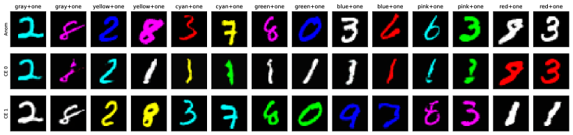
Figure 9: CEs for Col-MNIST and an anomaly detector trained with BCE (OE). For each normal definition, a different detector and CE generator was trained. In each subfigure, the first row shows anomalies, the other two corresponding counterfactuals for two different concepts. Each column is labeled with the corresponding combined normal class at the top.

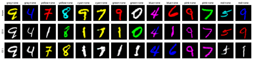
Figure 10: CEs for Col-MNIST and an anomaly detector trained with HSC (OE). For each normal definition, a different detector and CE generator was trained. In each subfigure, the first row shows anomalies, the other two corresponding counterfactuals for two different concepts. Each column is labeled with the corresponding combined normal class at the top.

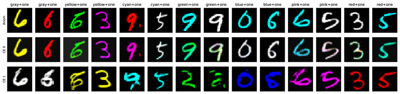
Figure 11: CEs for Col-MNIST and an anomaly detector trained with DSVDD. For each normal definition, a different detector and counterfactual generator was trained. In each subfigure, the first row shows anomalies, the other two corresponding counterfactuals for two different concepts. Each column is labeled with the corresponding combined normal class at the top.

Figures 12, 13, and 14 show CEs for MNIST, single classes being normal, and an AD trained with BCE, HSC, and DSVDD, respectively.

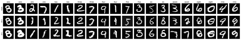
Figure 12: CEs for MNIST, diverse single normal classes, and an anomaly detector trained with BCE (OE). For each normal definition, a different detector and counterfactual generator was trained. In each subfigure, the first row shows anomalies, the other two corresponding counterfactuals for two different concepts. Each column is labeled with the corresponding single normal class at the top.

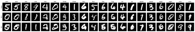
Figure 13: CEs for MNIST, diverse single normal classes, and an anomaly detector trained with HSC (OE). For each normal definition, a different detector and counterfactual generator was trained. In each subfigure, the first row shows anomalies, the other two corresponding counterfactuals for two different concepts. Each column is labeled with the corresponding single normal class at the top.

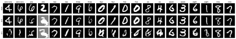
Figure 14: CEs for MNIST, diverse single normal classes, and an anomaly detector trained with DSVDD. For each normal definition, a different detector and counterfactual generator was trained. In each subfigure, the first row shows anomalies, the other two corresponding counterfactuals for two different concepts. Each column is labeled with the corresponding single normal class at the top.

Figures 15, 16, and 17 show CEs for CIFAR-10, single classes being normal, and an AD trained with BCE, HSC, and DSVDD, respectively.

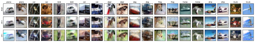
Figure 15: CEs for CIFAR-10, diverse single normal classes, and an anomaly detector trained with BCE (OE). For each normal definition, a different detector and counterfactual generator was trained. In each subfigure, the first row shows anomalies, the other two corresponding counterfactuals for two different concepts. Each column is labeled with the corresponding single normal class at the top.

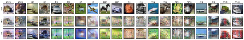
Figure 16: CEs for CIFAR-10, diverse single normal classes, and an anomaly detector trained with HSC (OE). For each normal definition, a different detector and counterfactual generator was trained. In each subfigure, the first row shows anomalies, the other two corresponding counterfactuals for two different concepts. Each column is labeled with the corresponding single normal class at the top.

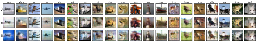
Figure 17: CEs for CIFAR-10, diverse single normal classes, and an anomaly detector trained with DSVDD. For each normal definition, a different detector and counterfactual generator was trained. In each subfigure, the first row shows anomalies, the other two corresponding counterfactuals for two different concepts. Each column is labeled with the corresponding single normal class at the top.

Figures 18, 19, and 20 show CEs for MNIST, class combinations being normal, and an AD trained with BCE, HSC, and DSVDD, respectively.

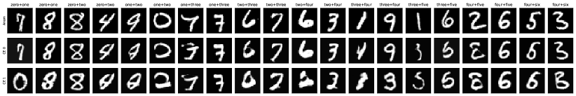
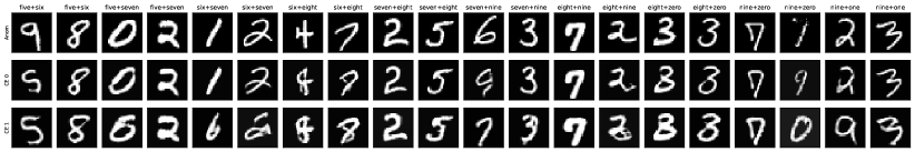
Figure 18: CEs for MNIST, diverse combined normal classes, and an anomaly detector trained with BCE (OE). For each normal definition, a different detector and counterfactual generator was trained. In each subfigure, the first row shows anomalies, the other two corresponding counterfactuals for two different concepts. Each column is labeled with the corresponding combined normal class at the top.

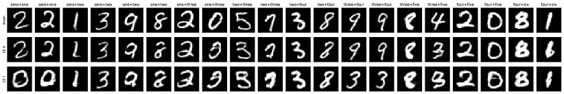
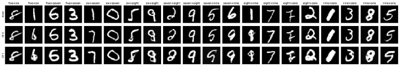
Figure 19: CEs for MNIST, diverse combined normal classes, and an anomaly detector trained with HSC (OE). For each normal definition, a different detector and counterfactual generator was trained. In each subfigure, the first row shows anomalies, the other two corresponding counterfactuals for two different concepts. Each column is labeled with the corresponding combined normal class at the top.

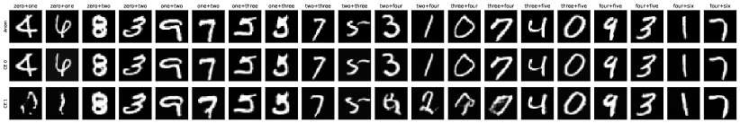
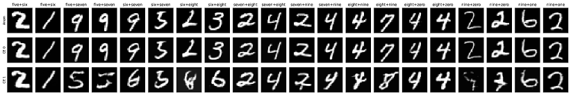
Figure 20: CEs for MNIST, diverse combined normal classes, and an anomaly detector trained with DSVDD. For each normal definition, a different detector and counterfactual generator was trained. In each subfigure, the first row shows anomalies, the other two corresponding counterfactuals for two different concepts. Each column is labeled with the corresponding combined normal class at the top.

Figures 21, 22, and 23 show CEs for CIFAR-10, class combinations being normal, and an AD trained with BCE, HSC, and DSVDD, respectively.

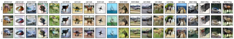
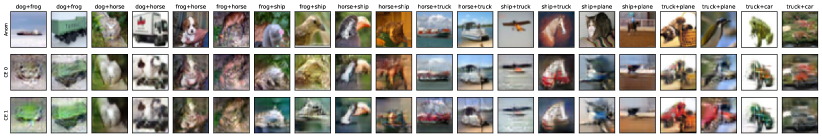
Figure 21: CEs for CIFAR-10, diverse combined normal classes, and an anomaly detector trained with BCE (OE). For each normal definition, a different detector and counterfactual generator was trained. In each subfigure, the first row shows anomalies, the other two corresponding counterfactuals for two different concepts. Each column is labeled with the corresponding combined normal class at the top.

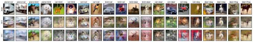
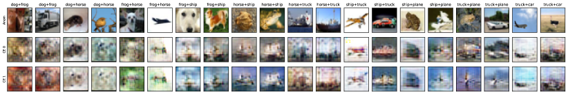
Figure 22: CEs for CIFAR-10, diverse combined normal classes, and an anomaly detector trained with HSC (OE). For each normal definition, a different detector and counterfactual generator was trained. In each subfigure, the first row shows anomalies, the other two corresponding counterfactuals for two different concepts. Each column is labeled with the corresponding combined normal class at the top.

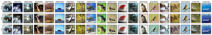
Figure 23: CEs for CIFAR-10, diverse combined normal classes, and an anomaly detector trained with DSVDD. For each normal definition, a different detector and counterfactual generator was trained. In each subfigure, the first row shows anomalies, the other two corresponding counterfactuals for two different concepts. Each column is labeled with the corresponding combined normal class at the top.

Figures 24, 25, and 26 show CEs for GTSDB, class combinations being normal, and an AD trained with BCE, HSC, and DSVDD, respectively.

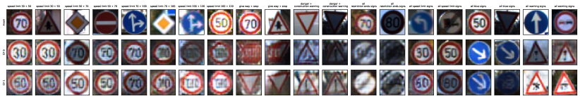
Figure 24: CEs for GTSDB and an anomaly detector trained with BCE OE. For each normal definition, a different detector and counterfactual generator was trained. In each subfigure, the first row shows anomalies, the other two corresponding counterfactuals for two different concepts. Each column is labeled with the corresponding combined normal class at the top.

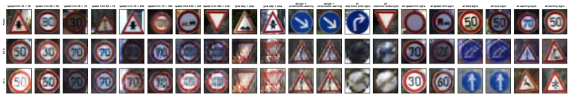
Figure 25: CEs for GTSDB and an anomaly detector trained with HSC OE. For each normal definition, a different detector and counterfactual generator was trained. In each subfigure, the first row shows anomalies, the other two corresponding counterfactuals for two different concepts. Each column is labeled with the corresponding combined normal class at the top.

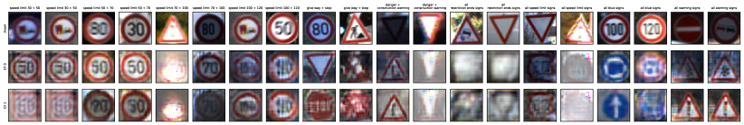
Figure 26: CEs for GTSDB and an anomaly detector trained with DSVDD. For each normal definition, a different detector and counterfactual generator was trained. In each subfigure, the first row shows anomalies, the other two corresponding counterfactuals for two different concepts. Each column is labeled with the corresponding combined normal class at the top.

References

- Abid et al. [2022] A. Abid, M. Yuksekgonul, and J. Zou. Meaningfully debugging model mistakes using conceptual counterfactual explanations. In International Conference on Machine Learning, pages 66–88. PMLR, 2022.
- Adebayo et al. [2018] J. Adebayo, J. Gilmer, M. Muelly, I. Goodfellow, M. Hardt, and B. Kim. Sanity checks for saliency maps. Advances in neural information processing systems, 31, 2018.
- Alqaraawi et al. [2020] A. Alqaraawi, M. Schuessler, P. Weiß, E. Costanza, and N. Berthouze. Evaluating saliency map explanations for convolutional neural networks: a user study. In Proceedings of the 25th international conference on intelligent user interfaces, pages 275–285, 2020.
- Angiulli et al. [2023] F. Angiulli, F. Fassetti, S. Nisticó, and L. Palopoli. Counterfactuals explanations for outliers via subspaces density contrastive loss. In International Conference on Discovery Science, pages 159–173. Springer, 2023.
- Baur et al. [2019] C. Baur, B. Wiestler, S. Albarqouni, and N. Navab. Deep autoencoding models for unsupervised anomaly segmentation in brain mr images. Lecture Notes in Computer Science, pages 161–169, 2019. ISSN 1611-3349. doi: 10.1007/978-3-030-11723-8_16.
- Bergmann et al. [2019] P. Bergmann, M. Fauser, D. Sattlegger, and C. Steger. Mvtec ad–a comprehensive real-world dataset for unsupervised anomaly detection. In Proceedings of the IEEE/CVF conference on computer vision and pattern recognition, pages 9592–9600, 2019.
- Birhane and Prabhu [2021] A. Birhane and V. U. Prabhu. Large image datasets: A pyrrhic win for computer vision? In 2021 IEEE Winter Conference on Applications of Computer Vision (WACV), pages 1536–1546. IEEE, 2021.
- Chandola et al. [2009] V. Chandola, A. Banerjee, and V. Kumar. Anomaly detection: A survey. ACM Computing Surveys, 41(3):1–58, 2009.
- Cheng et al. [2022] H. Cheng, D. Xu, S. Yuan, and X. Wu. Fine-grained anomaly detection in sequential data via counterfactual explanations. arXiv preprint arXiv:2210.04145, 2022.
- Cohen et al. [2017] G. Cohen, S. Afshar, J. Tapson, and A. Van Schaik. EMNIST: Extending MNIST to handwritten letters. In International Joint Conference on Neural Networks, pages 2921–2926, 2017.
- Datta et al. [2022a] D. Datta, F. Chen, and N. Ramakrishnan. Framing algorithmic recourse for anomaly detection. In Proceedings of the 28th ACM SIGKDD Conference on Knowledge Discovery and Data Mining, pages 283–293, 2022a.
- Datta et al. [2022b] D. Datta, F. Chen, and N. Ramakrishnan. Framing Algorithmic Recourse for Anomaly Detection. In Proceedings of the 28th ACM SIGKDD Conference on Knowledge Discovery and Data Mining, pages 283–293, Aug. 2022b. doi: 10.1145/3534678.3539344. URL http://arxiv.org/abs/2206.14384. arXiv:2206.14384 [cs, stat].
- De Vries et al. [2017] H. De Vries, F. Strub, J. Mary, H. Larochelle, O. Pietquin, and A. C. Courville. Modulating early visual processing by language. Advances in Neural Information Processing Systems, 30, 2017.
- Deecke et al. [2021] L. Deecke, L. Ruff, R. A. Vandermeulen, and H. Bilen. Transfer-based semantic anomaly detection. In International Conference on Machine Learning, pages 2546–2558. PMLR, 2021.
- Defard et al. [2021] T. Defard, A. Setkov, A. Loesch, and R. Audigier. Padim: a patch distribution modeling framework for anomaly detection and localization. In International Conference on Pattern Recognition, pages 475–489. Springer, 2021.
- Dehaene et al. [2020] D. Dehaene, O. Frigo, S. Combrexelle, and P. Eline. Iterative energy-based projection on a normal data manifold for anomaly localization. In International Conference on Learning Representations, 2020.
- Deng [2012] L. Deng. The mnist database of handwritten digit images for machine learning research. IEEE Signal Processing Magazine, 29(6):141–142, 2012.
- Dhurandhar et al. [2018] A. Dhurandhar, P.-Y. Chen, R. Luss, C.-C. Tu, P. Ting, K. Shanmugam, and P. Das. Explanations based on the missing: Towards contrastive explanations with pertinent negatives. Advances in neural information processing systems, 31, 2018.
- Fong and Vedaldi [2017] R. C. Fong and A. Vedaldi. Interpretable explanations of black boxes by meaningful perturbation. In Proceedings of the IEEE international conference on computer vision, pages 3429–3437, 2017.
- Ghandeharioun et al. [2021] A. Ghandeharioun, B. Kim, C.-L. Li, B. Jou, B. Eoff, and R. W. Picard. DISSECT: Disentangled Simultaneous Explanations via Concept Traversals. In International Conference on Learning Representations. OpenReview.net, 2021. doi: 10.48550/ARXIV.2105.15164. URL https://openreview.net/forum?id=qY79G8jGsep. Version Number: 4.
- Golan and El-Yaniv [2018] I. Golan and R. El-Yaniv. Deep anomaly detection using geometric transformations. In Advances in Neural Information Processing Systems, pages 9758–9769, 2018.
- Goodfellow et al. [2020] I. Goodfellow, J. Pouget-Abadie, M. Mirza, B. Xu, D. Warde-Farley, S. Ozair, A. Courville, and Y. Bengio. Generative adversarial networks. Communications of the ACM, 63(11):139–144, 2020.
- Görnitz et al. [2014] N. Görnitz, M. Kloft, K. Rieck, and U. Brefeld. Toward supervised anomaly detection. J. Artif. Intell. Res., 46:235–262, 2014. URL https://api.semanticscholar.org/CorpusID:9406699.
- Goyal et al. [2019] Y. Goyal, Z. Wu, J. Ernst, D. Batra, D. Parikh, and S. Lee. Counterfactual Visual Explanations. In Proceedings of the 36th International Conference on Machine Learning, pages 2376–2384. PMLR, May 2019. URL https://proceedings.mlr.press/v97/goyal19a.html.
- Gudovskiy et al. [2022] D. Gudovskiy, S. Ishizaka, and K. Kozuka. Cflow-ad: Real-time unsupervised anomaly detection with localization via conditional normalizing flows. In Proceedings of the IEEE/CVF Winter Conference on Applications of Computer Vision, pages 98–107, 2022.
- Guidotti [2022] R. Guidotti. Counterfactual explanations and how to find them: literature review and benchmarking. Data Mining and Knowledge Discovery, pages 1–55, 2022.
- Gupta et al. [2018] A. Gupta, J. Johnson, L. Fei-Fei, S. Savarese, and A. Alahi. Social GAN: Socially acceptable trajectories with generative adversarial networks. In CVPR, pages 2255–2264, 2018.
- Han et al. [2023] X. Han, L. Zhang, Y. Wu, and S. Yuan. Achieving counterfactual fairness for anomaly detection. In Pacific-Asia Conference on Knowledge Discovery and Data Mining, pages 55–66. Springer, 2023.
- Hanley and McNeil [1982] J. A. Hanley and B. J. McNeil. The meaning and use of the area under a receiver operating characteristic (roc) curve. Radiology, 143(1):29–36, 1982.
- Hartung et al. [2023] F. Hartung, B. J. Franks, T. Michels, D. Wagner, P. Liznerski, S. Reithermann, S. Fellenz, F. Jirasek, M. Rudolph, D. Neider, et al. Deep anomaly detection on tennessee eastman process data. Chemie Ingenieur Technik, 2023.
- He et al. [2016] K. He, X. Zhang, S. Ren, and J. Sun. Deep residual learning for image recognition. In Proceedings of the IEEE conference on computer vision and pattern recognition, pages 770–778, 2016.
- Hendrycks et al. [2019a] D. Hendrycks, M. Mazeika, and T. G. Dietterich. Deep anomaly detection with outlier exposure. In International Conference on Learning Representations, 2019a.
- Hendrycks et al. [2019b] D. Hendrycks, M. Mazeika, S. Kadavath, and D. Song. Using self-supervised learning can improve model robustness and uncertainty. In Advances in Neural Information Processing Systems, pages 15637–15648, 2019b.
- Heusel et al. [2017] M. Heusel, H. Ramsauer, T. Unterthiner, B. Nessler, and S. Hochreiter. Gans trained by a two time-scale update rule converge to a local nash equilibrium. Advances in neural information processing systems, 30, 2017.
- Houben et al. [2013] S. Houben, J. Stallkamp, J. Salmen, M. Schlipsing, and C. Igel. Detection of traffic signs in real-world images: The German Traffic Sign Detection Benchmark. In International Joint Conference on Neural Networks, number 1288, 2013.
- Krizhevsky et al. [2009] A. Krizhevsky, G. Hinton, et al. Learning multiple layers of features from tiny images. Technical report, Citeseer, 2009.
- Li et al. [2021] C.-L. Li, K. Sohn, J. Yoon, and T. Pfister. Cutpaste: Self-supervised learning for anomaly detection and localization. In Proceedings of the IEEE/CVF Conference on Computer Vision and Pattern Recognition, pages 9664–9674, 2021.
- Linardatos et al. [2020] P. Linardatos, V. Papastefanopoulos, and S. Kotsiantis. Explainable ai: A review of machine learning interpretability methods. Entropy, 23(1):18, 2020.
- Liu et al. [2020] W. Liu, R. Li, M. Zheng, S. Karanam, Z. Wu, B. Bhanu, R. J. Radke, and O. Camps. Towards visually explaining variational autoencoders. In Proceedings of the IEEE Conference on computer vision and pattern recognition, pages 8642–8651, 2020.
- Liznerski et al. [2021] P. Liznerski, L. Ruff, R. A. Vandermeulen, B. J. Franks, M. Kloft, and K.-R. Müller. Explainable deep one-class classification. In International Conference on Learning Representations, 2021.
- Liznerski et al. [2022] P. Liznerski, L. Ruff, R. A. Vandermeulen, B. J. Franks, K.-R. Müller, and M. Kloft. Exposing outlier exposure: What can be learned from few, one, and zero outlier images. Transactions on Machine Learning Research, 2022. URL https://openreview.net/forum?id=3v78awEzyB.
- Miyato and Koyama [2018] T. Miyato and M. Koyama. cgans with projection discriminator. In 6th International Conference on Learning Representations, ICLR 2018, Vancouver, BC, Canada, April 30 - May 3, 2018, Conference Track Proceedings. OpenReview.net, 2018. URL https://openreview.net/forum?id=ByS1VpgRZ.
- Miyato et al. [2018] T. Miyato, T. Kataoka, M. Koyama, and Y. Yoshida. Spectral normalization for generative adversarial networks. In 6th International Conference on Learning Representations, ICLR 2018, Vancouver, BC, Canada, April 30 - May 3, 2018, Conference Track Proceedings. OpenReview.net, 2018. URL https://openreview.net/forum?id=B1QRgziT-.
- Montavon et al. [2018] G. Montavon, W. Samek, and K.-R. Müller. Methods for interpreting and understanding deep neural networks. Digital Signal Processing, 73:1–15, 2018.
- Mothilal et al. [2020] R. K. Mothilal, A. Sharma, and C. Tan. Explaining machine learning classifiers through diverse counterfactual explanations. In Proceedings of the 2020 conference on fairness, accountability, and transparency, pages 607–617, 2020.
- Neuwirth [2022] R. J. Neuwirth. The EU artificial intelligence act: regulating subliminal AI systems. Taylor & Francis, 2022.
- Pearl [2009] J. Pearl. Causality. Cambridge university press, 2009.
- Reiss et al. [2021] T. Reiss, N. Cohen, L. Bergman, and Y. Hoshen. Panda: Adapting pretrained features for anomaly detection and segmentation. In Proceedings of the IEEE/CVF Conference on Computer Vision and Pattern Recognition, pages 2806–2814, 2021.
- Roth et al. [2022] K. Roth, L. Pemula, J. Zepeda, B. Schölkopf, T. Brox, and P. Gehler. Towards total recall in industrial anomaly detection. In Proceedings of the IEEE/CVF Conference on Computer Vision and Pattern Recognition, pages 14318–14328, 2022.
- Ruff et al. [2018] L. Ruff, R. A. Vandermeulen, N. Görnitz, L. Deecke, S. A. Siddiqui, A. Binder, E. Müller, and M. Kloft. Deep one-class classification. In International Conference on Machine Learning, volume 80, pages 4390–4399, 2018.
- Ruff et al. [2020] L. Ruff, R. A. Vandermeulen, N. Görnitz, A. Binder, E. Müller, K.-R. Müller, and M. Kloft. Deep semi-supervised anomaly detection. In International Conference on Learning Representations, 2020.
- Ruff et al. [2021] L. Ruff, J. R. Kauffmann, R. A. Vandermeulen, G. Montavon, W. Samek, M. Kloft, T. G. Dietterich, and K.-R. Müller. A unifying review of deep and shallow anomaly detection. Proceedings of the IEEE, 109(5):756–795, 2021.
- Samek et al. [2020] W. Samek, G. Montavon, S. Lapuschkin, C. J. Anders, and K.-R. Müller. Toward interpretable machine learning: Transparent deep neural networks and beyond. arXiv preprint arXiv:2003.07631, 2020.
- Selvaraju et al. [2017] R. R. Selvaraju, M. Cogswell, A. Das, R. Vedantam, D. Parikh, and D. Batra. Grad-cam: Visual explanations from deep networks via gradient-based localization. In Proceedings of the IEEE international conference on computer vision, pages 618–626, 2017.
- Singla et al. [2023] S. Singla, M. Eslami, B. Pollack, S. Wallace, and K. Batmanghelich. Explaining the black-box smoothly—a counterfactual approach. Medical Image Analysis, 84:102721, 2023.
- Sulem et al. [2022] D. Sulem, M. Donini, M. B. Zafar, F.-X. Aubet, J. Gasthaus, T. Januschowski, S. Das, K. Kenthapadi, and C. Archambeau. Diverse Counterfactual Explanations for Anomaly Detection in Time Series, Mar. 2022. URL http://arxiv.org/abs/2203.11103. arXiv:2203.11103 [cs, stat].
- Szegedy et al. [2015] C. Szegedy, W. Liu, Y. Jia, P. Sermanet, S. Reed, D. Anguelov, D. Erhan, V. Vanhoucke, and A. Rabinovich. Going deeper with convolutions. In Proceedings of the IEEE conference on computer vision and pattern recognition, pages 1–9, 2015.
- Tack et al. [2020] J. Tack, S. Mo, J. Jeong, and J. Shin. Csi: Novelty detection via contrastive learning on distributionally shifted instances. Advances in neural information processing systems, 33:11839–11852, 2020.
- Tax and Duin [2004] D. M. Tax and R. P. Duin. Support vector data description. Machine learning, 54(1):45–66, 2004.
- Venkataramanan et al. [2020] S. Venkataramanan, K.-C. Peng, R. V. Singh, and A. Mahalanobis. Attention guided anomaly localization in images. In European Conference on Computer Vision, pages 485–503. Springer, 2020.
- Wachter et al. [2017] S. Wachter, B. Mittelstadt, and C. Russell. Counterfactual explanations without opening the black box: Automated decisions and the gdpr. Harv. JL & Tech., 31:841, 2017.
- Wang et al. [2021] S. Wang, L. Wu, L. Cui, and Y. Shen. Glancing at the patch: Anomaly localization with global and local feature comparison. In Proceedings of the IEEE/CVF Conference on Computer Vision and Pattern Recognition, pages 254–263, 2021.
- Zagoruyko and Komodakis [2016] S. Zagoruyko and N. Komodakis. Wide residual networks. In British Machine Vision Conference, 2016.
- Zhang et al. [2018] J. Zhang, S. A. Bargal, Z. Lin, J. Brandt, X. Shen, and S. Sclaroff. Top-down neural attention by excitation backprop. International Journal of Computer Vision, 126(10):1084–1102, 2018.
- Zhu et al. [2017] J.-Y. Zhu, T. Park, P. Isola, and A. A. Efros. Unpaired image-to-image translation using cycle-consistent adversarial networks. In Proceedings of the IEEE international conference on computer vision, pages 2223–2232, 2017.
- Zintgraf et al. [2017] L. M. Zintgraf, T. S. Cohen, T. Adel, and M. Welling. Visualizing deep neural network decisions: Prediction difference analysis. arXiv preprint arXiv:1702.04595, 2017.