Parallelized Midpoint Randomization for Langevin Monte Carlo

Abstract

We explore the sampling problem within the framework where parallel evaluations of the gradient of the log-density are feasible. Our investigation focuses on target distributions characterized by smooth and strongly log-concave densities. We revisit the parallelized randomized midpoint method and employ proof techniques recently developed for analyzing its purely sequential version. Leveraging these techniques, we derive upper bounds on the Wasserstein distance between the sampling and target densities. These bounds quantify the runtime improvement achieved by utilizing parallel processing units, which can be considerable.

[inst1]organization=CREST/ENSAE Paris,addressline=5 Av. Le Chatelier, city=Palaiseau, postcode=91120, country=France

1 Introduction

Parallel computing is widespread in modern machine learning and scientific computing, allowing for the simultaneous execution of multiple tasks, resulting in faster processing times [1, 2, 3]. This is particularly crucial for applications involving intensive calculations, such as scientific simulations or big data analysis. Moreover, parallel computing optimizes resource utilization by distributing tasks across multiple processors or computers, reducing the time and energy required for a given task and enhancing efficiency and cost-effectiveness.

Optimization problems, particularly in machine learning and scientific computing, often involve large datasets and complex objective functions. Solving such problems on a single processor can be time-consuming. In the field of optimization, leveraging parallel computing to expedite the solution of computationally expensive problems is a common practice. Many optimization algorithms, such as gradient descent, can be parallelized [4, 5]. The workload is distributed among processors, with each processor updating a portion of the model parameters based on its subset of the data. In deep learning, mini-batch stochastic gradient descent is often used [6, 7]. Parallelization involves distributing these mini-batches across different processors, allowing for efficient model training.

On the other hand, traditional sampling methods often involve sequential processes, which may become computationally burdensome for large datasets or complex models. Parallel computing addresses this challenge by distributing the workload across multiple processors, enabling the concurrent execution of sampling tasks and enhancing computational efficiency, thus accelerating the generation of samples in statistical applications. Over the past few decades, there has been substantial research on parallel computing for sampling methods, with a notable focus on Monte Carlo methods in Monte Carlo simulations [8, 9, 10], particularly in the context of Markov chain Monte Carlo (MCMC) [11, 12, 13, 14].

However, despite the intrinsic analogy between sampling and optimization [15, 16, 17, 18], and the extensive studies in parallel schemes for Monte Carlo methods, the application of parallel computing to Langevin Monte Carlo (LMC) [19, 20, 21, 22, 23, 24, 25, 26, 27, 28, 29] remains relatively unexplored, given that LMC is one of the canonical sampling algorithms in MCMC. An exception to this is highlighted in the recent work by [31], where they introduce a parallelized version of the midpoint randomization for kinetic Langevin Monte Carlo [32, 33, 31, 34, 35, 36]. This innovative approach notably accelerates the sampling process. Building upon the foundations laid by [31], we explore parallel computing for the midpoint randomization method in Langevin Monte Carlo [37, 38]. Our contributions can be summarized as follows.

• Parallelized Randomized Midpoint Method for Langevin Monte Carlo   We introduce a parallel computing scheme for the randomized midpoint method applied to Langevin Monte Carlo in Algorithm 1. We derive the corresponding convergence guarantees in ${\sf W}_{2}$-distance in Theorem 1, providing small constants and explicit dependence on the initialization and choice of the parameters.

• Parallelized Randomized Midpoint Method for kinetic Langevin Monte Carlo   In Theorem 2, we present a comprehensive analysis of the parallel computing for the randomized midpoint method applied to kinetic Langevin Monte Carlo. Compared to previous work, our results offer a) small constants and the explicit dependence on the initialization, b) does not require the initialization to be at minimizer of the potential, c) removes the linear dependence on the sample size, which serves as a crucial step towards extending the method to non-convex potentials.

In summary, our work offers a thorough analysis of the parallelized randomized midpoint method applied to Langevin Monte Carlo. This study intends to provide valuable insights and to contribute to the advancement of parallel computing techniques in the context of sampling.

Notation. Denote the $p$-dimensional Euclidean space by $\mathbb{R}^{p}$. The letter $\boldsymbol{\theta}$ denotes the deterministic vector and its calligraphic counterpart $\boldsymbol{\vartheta}$ denotes the random vector. We use $\mathbf{I}_{p}$ and $\mathbf{0}_{p}$ to denote, respectively, the $p\times p$ identity and zero matrices. Define the relations $\mathbf{A}\preccurlyeq\mathbf{B}$ and $\mathbf{B}\succcurlyeq\mathbf{A}$ for two symmetric $p\times p$ matrices $\mathbf{A}$ and $\mathbf{B}$ to mean that $\mathbf{B}-\mathbf{A}$ is semi-definite positive. The gradient and the Hessian of a function $f:\mathbb{R}^{p}\rightarrow\mathbb{R}$ are denoted by $\nabla f$ and $\nabla^{2}f$, respectively. Given any pair of measures $\mu$ and $\nu$ defined on $(\mathbb{R}^{p},\mathcal{B}(\mathbb{R}^{p}))$, the Wasserstein-2 distance between $\mu$ and $\nu$ is defined as

$${\sf W}_{2}(\mu,\nu)=\Big{(}\inf_{\varrho\in\Gamma(\mu,\nu)}\int_{\mathbb{R}^{p}\times\mathbb{R}^{p}}\|\boldsymbol{\theta}-\boldsymbol{\theta}^{\prime}\|_{2}^{2}\,{\rm d}\varrho(\boldsymbol{\theta},\boldsymbol{\theta}^{\prime})\Big{)}^{1/2},$$ (1)

where the infimum is taken over all joint distributions $\varrho$ that have $\mu$ and $\nu$ as marginals. The ceiling function maps $x\in\mathbb{R}$ to the smallest integer greater than or equal to $x$, denoted by $\lceil{x}\rceil.$ Given two probability distributions $\nu,\mu$, the Kullback-Leibler divergence of $\nu$ from $\mu$, is defined as $D_{\sf KL}(\mu||\nu).$

2 Parallelized randomized midpoint discretization: the vanilla Langevin diffusion

The goal is to sample a random vector in $\mathbb{R}^{p}$ according to a given distribution $\pi$ of the form

$$\pi(\boldsymbol{\theta})\propto\exp\{-f(\boldsymbol{\theta})\},\qquad\boldsymbol{\theta}\in\mathbb{R}^{p},$$ (2)

with a function $f:\mathbb{R}^{p}\to\mathbb{R}$, referred to as the potential. Throughout the paper, we assume that the potential function $f$ is $M$-smooth and $m$-strongly convex for some constants $0<m\leqslant M<\infty$.

Assumption 1.

The function $f:\mathbb{R}^{p}\to\mathbb{R}$ is twice differentiable, and its Hessian matrix $\nabla^{2}f$ satisfies

$$m\mathbf{I}_{p}\preccurlyeq\nabla^{2}f(\boldsymbol{\theta})\preccurlyeq M\mathbf{I}_{p},\qquad\forall\boldsymbol{\theta}\in\mathbb{R}^{p}.$$ (3)

Let $\boldsymbol{\vartheta}_{0}$ be a random vector drawn from a distribution $\nu$ on $\mathbb{R}^{p}$ and let $\boldsymbol{W}=(\boldsymbol{W}_{t}:t\geqslant 0)$ be a $p$-dimensional Brownian motion independent of $\boldsymbol{\vartheta}_{0}$. Using the potential $f$, the random variable $\boldsymbol{\vartheta}_{0}$ and the process $\boldsymbol{W}$, one can define the stochastic differential equation

$$d\boldsymbol{L}_{t}^{\sf LD}=-\nabla f(\boldsymbol{L}_{t}^{\sf LD})\,dt+\sqrt{2}\,{\rm d}\boldsymbol{W}_{t},\quad t\geqslant 0,\qquad\boldsymbol{L}^{\sf LD}_{0}=\boldsymbol{\vartheta}_{0}.$$ (4)

This equation has a unique strong solution, which is a continuous-time Markov process, termed Langevin diffusion. Under some further assumptions on $f$, such as strong convexity or dissipativity, the Langevin diffusion is ergodic, geometrically mixing and has $\pi$ as its unique invariant density [39]. Furthermore, we can sample from the distribution defined by $\pi$ by using a suitable discretization of the Langevin diffusion. The Langevin Monte Carlo (LMC) method is based on this idea, combining the aforementioned considerations with the Euler discretization. Specifically, for small values of $h\geqslant 0$ and $\Delta_{h}\boldsymbol{W}_{t}=\boldsymbol{W}_{t+h}-\boldsymbol{W}_{t}$, the following approximation holds

$$\boldsymbol{L}^{\sf LD}_{t+h} =\boldsymbol{L}^{\sf LD}_{t}-\int_{0}^{h}\nabla f(\boldsymbol{L}_{t+s}^{\sf LD})\,{\rm d}s+\sqrt{2}\;\Delta_{h}\boldsymbol{W}_{t}\approx\boldsymbol{L}_{t}^{\sf LD}-h\nabla f(\boldsymbol{L}_{t}^{\sf LD})+\sqrt{2}\;\Delta_{h}\boldsymbol{W}_{t}.$$ (5)

By repeatedly applying this approximation, we can construct a Markov chain $(\boldsymbol{\vartheta}^{\sf LMC}_{k}:k\in\mathbb{N})$ that converges in distribution to the target $\pi$ as $h$ goes to zero. More precisely, $\boldsymbol{\vartheta}^{\sf LMC}_{k}\approx\boldsymbol{L}^{\sf LD}_{kh}$, for $k\in\mathbb{N}$, is given by

$$\boldsymbol{\vartheta}_{k+1}^{\sf LMC}=\boldsymbol{\vartheta}_{k}^{\sf LMC}-h\nabla f(\boldsymbol{\vartheta}_{k}^{\sf LMC})+\sqrt{2}\,(\boldsymbol{W}_{(k+1)h}-\boldsymbol{W}_{kh}).$$ (6)

It should be noted that the Brownian motion employed in (6) does not necessarily have to coincide with that utilized in the Langevin diffusion; it might be useful to opt for an alternative Brownian motion with more favorable “coupling” properties. However, all the proofs presented in this work are contingent upon synchronous sampling. That is, the discrete-time processes and their continuous-time counterparts necessitate the utilization of the same Brownian motion. Therefore, for the sake of consistency and clarity, we maintain the notation $\boldsymbol{W}$ throughout this discussion, both in (6) and (4).

Let $U$ be a random variable uniformly distributed in $[0,1]$ and independent of the Brownian motion $\boldsymbol{W}$. The randomized midpoint method exploits the approximation

$$\boldsymbol{L}^{\sf LD}_{t+h} =\boldsymbol{L}^{\sf LD}_{t}-\int_{0}^{h}\nabla f(\boldsymbol{L}^{\sf LD}_{t+s})\,{\rm d}s+\sqrt{2}\;\Delta_{h}\boldsymbol{W}_{t}$$ (7)

$$\approx\boldsymbol{L}^{\sf LD}_{t}-h\nabla f(\boldsymbol{L}^{\sf LD}_{t+hU})+\sqrt{2}\;\Delta_{h}\boldsymbol{W}_{t}.$$

The noise counterpart of $\boldsymbol{\zeta}_{k}$ in this case is $\boldsymbol{\zeta}_{k}^{\sf R}=\int_{0}^{h}\nabla f(\boldsymbol{L}^{\sf LD}_{kh+s})\,{\rm d}s-\nabla f(\boldsymbol{L}^{\sf LD}_{kh+Uh})$. It is clearly centered and uncorrelated with all the random vectors independent of $U$ such as $\boldsymbol{L}^{\sf LD}_{kh}$, $\boldsymbol{\vartheta}^{\sf LMC}_{k}$ and the gradient of $f$ evaluated at these points.

Let us now describe an alternative method for approximating the integral $\int_{0}^{h}\nabla f(\boldsymbol{L}_{t+s}^{\sf LD})\,{\rm d}s$, as proposed in [31]. This approach offers substantial reductions in running time through the parallelization of computations. The interval $[0,h]$ is divided into $R$ segments, each of length $\frac{h}{R}$. Choosing $U_{r}$ uniformly from the $r$-th interval $\big{[}\frac{r-1}{R},\frac{r}{R}\big{]}$ for $r=1,\dots,R$, the approximation within each interval is given by

$$\int_{0}^{h}\nabla f(\boldsymbol{L}_{t+s}^{\sf LD})\,{\rm d}s=\sum_{r=1}^{R}\int_{\frac{r-1}{R}h}^{\frac{r}{R}h}\nabla f(\boldsymbol{L}_{t+s}^{\sf LD})\,{\rm d}s\approx\sum_{r=1}^{R}\frac{h}{R}\nabla f(\boldsymbol{L}^{\sf LD}_{t+hU_{r}}).$$ (8)

Assume that there exists an approximation $\boldsymbol{\vartheta}_{k}$ of $\boldsymbol{L}^{\sf LD}$ at time $t=kh$ and the aim is to move to $t+h=(k+1)h$ using relations (7) and (8). This requires an approximation to the finite sequence $(\boldsymbol{L}^{\sf LD}_{t+hU_{1}},\ldots,\boldsymbol{L}^{\sf LD}_{t+hU_{R}})$. A rough approximation, used as an initial step is $(\boldsymbol{\vartheta}_{k},\ldots,\boldsymbol{\vartheta}_{k})\in(\mathbb{R}^{p})^{R}$. A small number $Q$ of sequential steps are then performed, updating each approximation $\boldsymbol{\vartheta}^{(q,r)}_{k}$ of $\boldsymbol{L}^{\sf LD}_{t+hU_{r}}$, for $r=1,\ldots,R$, in parallel. Each update relies only on the previous step’s values $\{\boldsymbol{\vartheta}^{(q-1,j)}_{k}\}_{j=1}^{r}$, ensuring parallelism. Since, similar to the approximation in (8), it holds that

$$L_{t+hU_{r}}^{\sf LD} =L_{t}^{\sf LD}-\sum_{j=1}^{r-1}\int_{\frac{j-1}{R}h}^{\frac{j}{R}h}\nabla f(\boldsymbol{L}_{t+s}^{\sf LD})\,{\rm d}s-\int_{\frac{r-1}{R}h}^{hU_{r}}\nabla f(\boldsymbol{L}_{t+s}^{\sf LD})\,{\rm d}s+\sqrt{2}\,\Delta_{hU_{r}}\boldsymbol{W}_{t}$$ (9)

$$\approx L_{t}^{\sf LD}-\sum_{j=1}^{r-1}\frac{h}{R}\nabla f(\boldsymbol{L}^{\sf LD}_{t+hU_{j}})-h(U_{r}-\tfrac{r-1}{R})\nabla f(\boldsymbol{L}^{\sf LD}_{t+hU_{r}})+\sqrt{2}\,\Delta_{hU_{r}}\boldsymbol{W}_{t},$$ (10)

the update rule for $\boldsymbol{\vartheta}_{k}^{(q,r)}$ proposed by [31] is defined as follows

$$\boldsymbol{\vartheta}^{(q,r)}_{k}=\boldsymbol{\vartheta}_{k}-\sum_{j=1}^{r-1}\frac{h}{R}\nabla f(\boldsymbol{\vartheta}^{(q-1,j)})-h(U_{r}-\tfrac{r-1}{R})\nabla f(\boldsymbol{\vartheta}^{(q-1,r)})+\sqrt{2}\,\Delta_{hU_{r}}\boldsymbol{W}_{t}.$$ (11)

This leads to the parallelized version of RLMC, referred to as pRLMC, the formal definition of which is provided in Algorithm 1. For simplicity, the superscript $\sf pRLMC$ is omitted therein. Figure 1 illustrates this algorithm.

Algorithm 1 Parallelized RLMC

Input: number of parallel steps $R$, number of sequential iterations $Q$, step size $h$, number of iterations $K$, initial point $\boldsymbol{\vartheta}_{0}.$
Output: iterate $\boldsymbol{\vartheta}_{K+1}$

1:for $k=1$ to $K$ do

2:     Draw $U_{kr}$ uniformly from $\big{[}\frac{r-1}{R},\frac{r}{R}\big{]}$, $r=1,\dots,R$.

3:     Generate $\boldsymbol{\xi}_{kr}=\boldsymbol{W}_{(k+U_{kr})h}-\boldsymbol{W}_{kh},r=1,\dots,R.$

4:     Set $\boldsymbol{\vartheta}_{k}^{(0,r)}=\boldsymbol{\vartheta}_{k},r=1,\dots,R$.

5:     for $q=1$ to $Q-1$ do

6:         for $r=1$ to $R$ in parallel do                                    

7:              $a_{kj}=\min\{\frac{1}{R},U_{kr}-\frac{j-1}{R}\},j=1,\dots,r$

8:              $\boldsymbol{\vartheta}_{k}^{(q,r)}=\boldsymbol{\vartheta}_{k}-h\sum_{j=1}^{r}a_{kj}\nabla f\big{(}\boldsymbol{\vartheta}_{k}^{(q-1,j)}\big{)}+\sqrt{2}\boldsymbol{\xi}_{kr}$.

9:         end for

10:     end for

11:     $\boldsymbol{\vartheta}_{k+1}=\boldsymbol{\vartheta}_{k}-\frac{h}{R}\sum_{r=1}^{R}\nabla f\big{(}\boldsymbol{\vartheta}_{k}^{(Q-1,r)}\big{)}+\sqrt{2}(\boldsymbol{W}_{(k+1)h}-\boldsymbol{W}_{kh})$.

12:end for

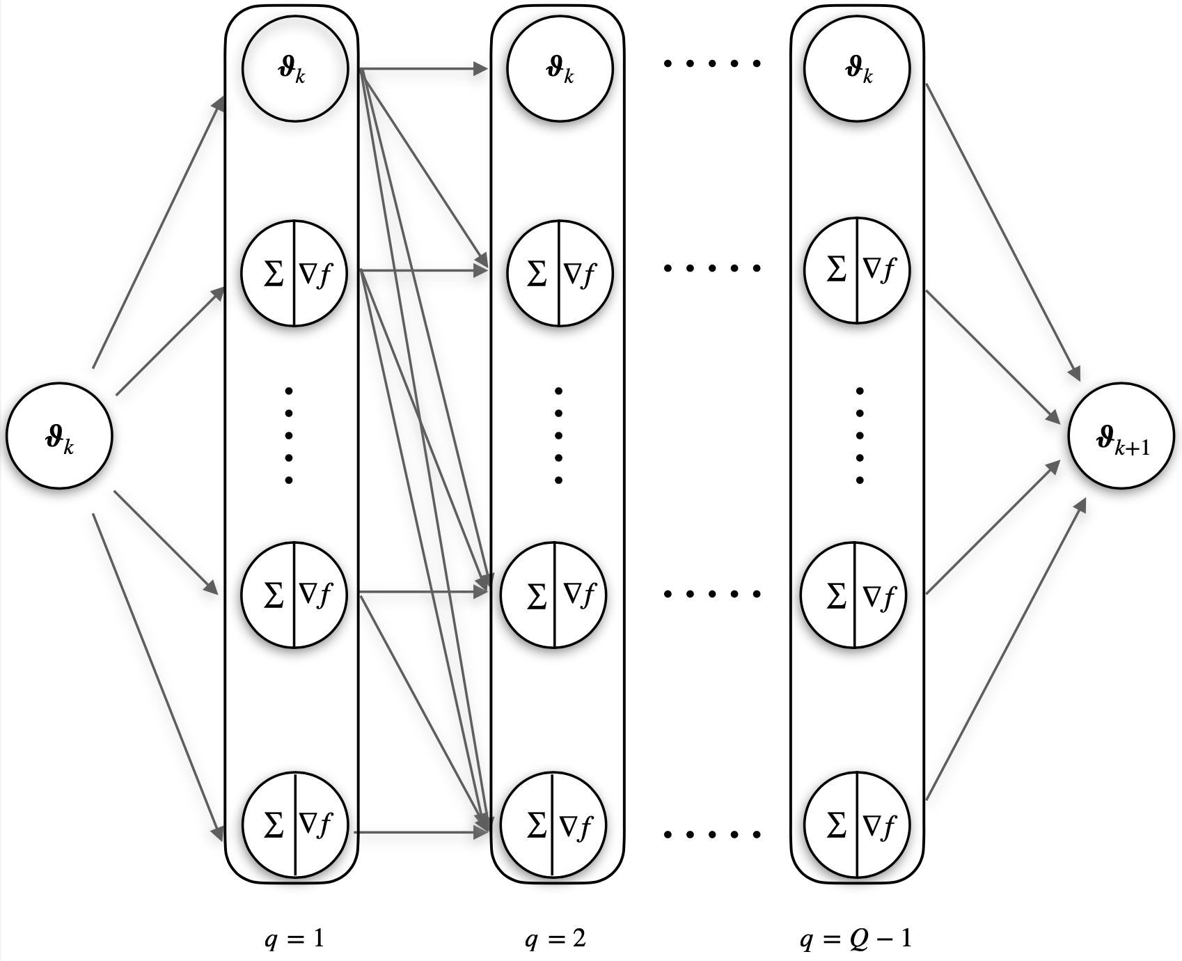
Figure 1: Visualization of Parallelized RLMC.

We state in the following the theoretical guarantee for the proposed parallelized RLMC algorithm (all proofs are deferred to the supplementary materials).

Theorem 1.

Assume the function $f:\mathbb{R}^{p}\to\mathbb{R}$ satisfies Assumption 1. Let $h$ be such that $Mh\leqslant 1/10$. Then, for every $n\geqslant 1$, the the distribution $\nu_{n}=\nu_{n}^{\textup{\sf pRLMC}}$ of $\boldsymbol{\vartheta}_{n}^{\textup{\sf pRLMC}}$ satisfies

$${\sf W}_{2}(\nu_{n},\pi) \leqslant\Big{(}1+\sqrt{\kappa Mh}\big{(}0.82(Mh)^{Q-1}+0.94Mh/R\big{)}\Big{)}e^{-mnh/2}{\sf W}_{2}(\nu_{0},\pi)$$ (12)

$$\qquad+\sqrt{\kappa Mh}\big{(}3.98(Mh)^{Q-1}+6.91Mh/\sqrt{R}\big{)}\sqrt{p/m}.$$ (13)

This result recovers the convergence rate presented in Theorem 1 in [38] for RLMC algorithm, with $R=1$ and $Q=2$. We then state the implication of this bound, providing insight into the number of iterations and parallel steps to attain a predetermined level of accuracy.

Corollary 1.

Let $\varepsilon\in(0,1)$ be a small number. If we choose the initial distribution $\nu_{0}$ to be the Dirac measure at the minimizer of $f$, denoted by $\boldsymbol{\theta}^{*}$, set $R=\lceil{1.54\kappa/\varepsilon^{2}}\rceil$, $Q=\lceil{0.22\log R}\rceil+1$, the step size $h>0$ and $n\in\mathbb{N}$ so that

$$Mh\leqslant 0.1,\quad\text{and}\quad n\geqslant 20\kappa\log(2/\varepsilon)\,,$$ (14)

then we have ${\sf W}_{2}(\nu_{n}^{\sf pRLMC},\pi)\leqslant\varepsilon\sqrt{p/m}$ after $nQ$ iterations, each of which involves $R=\lceil{1.54\kappa/\varepsilon^{2}}\rceil$ parallel queries of the gradient information $\nabla f$.

To our knowledge, this marks the first investigation into the error analysis of the parallelized RLMC algorithm. As this work neared completion, we became aware of the paper [30], which explores similar themes of accelerating Langevin process-based sampling methods through parallel gradient computations. A detailed comparison of our work with [30] is deferred to Section 4.

3 Parallelized Randomized midpoint method for the kinetic Langevin diffusion

In this section, we revisit the parallelization of the randomized midpoint method for the kinetic Langevin process (RKLMC), introduced and studied in [31]. We aim to provide a lucid quantification of the complexity bound. Recall that the kinetic Langevin process $\boldsymbol{L}^{\textup{\sf KLD}}$ is a solution to a second-order stochastic differential equation that can be informally written as

$${\textstyle\frac{1}{\gamma}}\ddot{\boldsymbol{L}}_{t}^{\sf KLD}+\dot{\boldsymbol{L}}_{t}^{\sf KLD}=-\nabla f(\boldsymbol{L}_{t}^{\sf KLD})+\sqrt{2}\,\dot{\boldsymbol{W}}_{t},$$ (15)

with initial conditions $\boldsymbol{L}_{0}^{\sf KLD}=\boldsymbol{\vartheta}_{0}$ and $\dot{\boldsymbol{L}}_{0}^{\sf KLD}=\boldsymbol{v}_{0}$. In (15), $\gamma>0$, $\boldsymbol{W}$ is a standard $p$-dimensional Brownian motion and dots are used to designatex derivatives with respect to time $t\geqslant 0$. This can be formalized using Itô’s calculus and introducing the velocity field $\boldsymbol{V}^{\sf KLD}$ so that the joint process $(\boldsymbol{L}^{\sf KLD},\boldsymbol{V}^{\sf KLD})$ satisfies

$${\rm d}\boldsymbol{L}^{\sf KLD}_{t}=\boldsymbol{V}_{t}^{\sf KLD}\,{\rm d}t;\quad\tfrac{1}{\gamma}{\rm d}\boldsymbol{V}^{\sf KLD}_{t}=-\big{(}\boldsymbol{V}_{t}^{\sf KLD}+\nabla f(\boldsymbol{L}_{t}^{\sf KLD})\big{)}\,{\rm d}t+\sqrt{2}\,{\rm d}\boldsymbol{W}_{t}.$$ (16)

Similar to the vanilla Langevin diffusion (4), the kinetic Langevin diffusion $(\boldsymbol{L}^{\sf KLD},\boldsymbol{V}^{\sf KLD})$ is a Markov process that exhibits ergodic properties when the potential $f$ is strongly convex (see [40] and references therein). The invariant density of this process is given by

$$p_{*}(\boldsymbol{\theta}_{,}\boldsymbol{v})\propto\exp\{-f(\boldsymbol{\theta})-{\textstyle\frac{1}{2\gamma}}\|\boldsymbol{v}\|^{2}\},\qquad\text{for all}\quad\boldsymbol{\theta},\boldsymbol{v}\in\mathbb{R}^{p}.$$ (17)

Note that the marginal of $p_{*}$ corresponds to $\boldsymbol{\theta}$ coincides with the target density $\pi$.

To discretize this continuous-time process and make it applicable to the sampling problem, [31] proposed the following procedure: at each iteration $k=1,2,\ldots$,

1. randomly, and independently of all the variables generated at the previous steps, generate random vectors $(\boldsymbol{\xi}_{k}^{\prime},\boldsymbol{\xi}^{\prime\prime}_{k},\boldsymbol{\xi}_{k}^{\prime\prime\prime})$ and a random variable $U_{k}$ such that

   • $U_{k}$ is uniformly distributed in $[0,1]$,

   • conditionally to $U_{k}=u$, $(\boldsymbol{\xi}_{k}^{\prime},\boldsymbol{\xi}^{\prime\prime}_{k},\boldsymbol{\xi}^{\prime\prime\prime}_{k})$ has the same joint distribution as $\big{(}\boldsymbol{B}_{u}-e^{-\gamma hu}\boldsymbol{G}_{u},\boldsymbol{B}_{1}-e^{-\gamma h}\boldsymbol{G}_{1},\gamma e^{-\gamma h}\boldsymbol{G}_{1}\big{)}$, where $\boldsymbol{B}$ is a $p$-dimensional Brownian motion and $\boldsymbol{G}_{t}=\int_{0}^{t}e^{\gamma hs}\,{\rm d}\boldsymbol{B}_{s}$.

2. set $\psi(x)=(1-e^{-x})/x$ and define the $(k+1)$-th iterate of $\boldsymbol{\vartheta}^{\sf RKLMC}$ by

   $$\boldsymbol{\vartheta}_{k+U} =\boldsymbol{\vartheta}_{k}+U_{k}h\psi(\gamma U_{k}h)\boldsymbol{v}_{k}-{U_{k}h}\big{(}1-\psi(\gamma U_{k}h)\big{)}\nabla f(\boldsymbol{\vartheta}_{k})+\sqrt{2h}\,\boldsymbol{\xi}^{\prime}_{k}$$ (18)

   $$\boldsymbol{\vartheta}_{k+1} =\boldsymbol{\vartheta}_{k}+h\psi(\gamma h)\boldsymbol{v}_{k}-\gamma h^{2}(1-U_{k})\psi\big{(}\gamma h(1-U_{k})\big{)}\nabla f(\boldsymbol{\vartheta}_{k+U})+\sqrt{2h}\boldsymbol{\xi}^{\prime\prime}_{k}$$ (19)

   $$\boldsymbol{v}_{k+1} =e^{-\gamma h}\boldsymbol{v}_{k}-{\gamma}he^{-\gamma h(1-U_{k})}\nabla f(\boldsymbol{\vartheta}_{k+U})+\sqrt{2h}\,\boldsymbol{\xi}^{\prime\prime\prime}_{k}.$$ (20)

The formal definition of the parallelized RKLMC algorithm is outlined in [31]. This algorithm is referred to as pRKLMC, and for the convenience of the readers, we restate it in Algorithm 2. To ease the notation, we omit the superscript $\sf pRKLMC$ therein.

Algorithm 2 Parallelized RKLMC

Input: number of parallel steps $R$, number of sequential iterations $Q$, step size $h$, friction coefficient $\gamma$, number of iterations $K$, initial points $\boldsymbol{v}_{0}$ and $\boldsymbol{\vartheta}_{0}.$
Output: iterates $\boldsymbol{\vartheta}_{K+1}$ and $\boldsymbol{v}_{K+1}$

1:for $k=1$ to $K$ do

2:     Draw $U_{k1},\dots,U_{kR}$ uniformly from $\big{[}0,\frac{1}{R}\big{]},\dots,\big{[}\frac{R-1}{R},1\big{]},$ respectively.

3:     Generate $\bar{\boldsymbol{W}}_{s}=\boldsymbol{W}_{kh+s}-\boldsymbol{W}_{kh}$

4:     Generate $\boldsymbol{\xi}_{kr}=\int_{0}^{U_{kr}h}\big{(}1-e^{-\gamma(U_{kr}h-s)}\big{)}d\bar{\boldsymbol{W}}_{s},r=1,\dots,R$.

5:     Set $\boldsymbol{\vartheta}_{k}^{(0,r)}=\boldsymbol{\vartheta}_{k},r=1,\dots,R$.

6:     for $q=1$ to $Q-1$ do

7:         for $r=1$ to $R$ in parallel do                                            

8:              $a_{kr}=\frac{1-e^{-\gamma hU_{kr}}}{\gamma}.$

9:              $b_{kj}=\int_{\frac{(j-1)h}{R}}^{h\min(\frac{j}{R},U_{kr})}(1-e^{-\gamma(U_{kr}h-s)})ds,j=1,\dots,r.$

10:              $\boldsymbol{\vartheta}_{k}^{(q,r)}=\boldsymbol{\vartheta}_{k}+a_{kr}\boldsymbol{v}_{k}-\sum_{j=1}^{r}b_{kj}\nabla f\big{(}\boldsymbol{\vartheta}_{k}^{(q-1,j)}\big{)}+\sqrt{2}\boldsymbol{\xi}_{kr}.$

11:         end for

12:     end for

13:     $\boldsymbol{\vartheta}_{k+1}=\boldsymbol{\vartheta}_{k}+\frac{1-e^{-\gamma h}}{\gamma}\boldsymbol{v}_{k}-\sum_{r=1}^{R}\frac{h}{R}(1-e^{-\gamma h(1-U_{kr})})\nabla f\big{(}\boldsymbol{\vartheta}_{k}^{(Q-1,r)}\big{)}+\sqrt{2}\int_{0}^{h}\big{(}1-e^{-\gamma(h-s)}\big{)}d\bar{\boldsymbol{W}}_{s}$.

14:     $\boldsymbol{v}_{k+1}=e^{-\gamma h}\boldsymbol{v}_{k}-\gamma\sum_{r=1}^{R}\frac{h}{R}e^{-\gamma h(1-U_{kr})}\nabla f\big{(}\boldsymbol{\vartheta}_{k}^{(Q-1,r)}\big{)}+\sqrt{2}\gamma\int_{0}^{h}e^{-\gamma(h-s)}d\bar{\boldsymbol{W}}_{s}$.

15:end for

In the following theorem, we present an upper bound of the ${\sf W}_{2}$ error for the parallelization of the RKLMC algorithm.

Theorem 2.

Let $f:\mathbb{R}^{p}\to\mathbb{R}$ be a function satisfying Assumption 1. Let $\boldsymbol{\theta}_{*}=\arg\min_{\boldsymbol{\theta}\in\mathbb{R}^{p}}f(\boldsymbol{\theta})$ be the minimizer of $f$ and assume that $f(\boldsymbol{\theta}_{*})=0$. Choose the parameters $\gamma$ and $h$ so that $\gamma\geqslant 5M$, and ${\kappa\big{(}\frac{(\gamma Mh^{2})^{3}}{R^{2}}+(\gamma Mh^{2})^{2Q-1}\big{)}}\leqslant 10^{-4},$ where $\kappa=M/m$. Assume that $\boldsymbol{\vartheta}_{0}$ is independent of $\boldsymbol{v}_{0}$ and that $\boldsymbol{v}_{0}\sim\mathcal{N}_{p}(0,\gamma\mathbf{I}_{p})$. Then, for any $n\geqslant 1$, the distribution $\nu_{n}=\nu_{n}^{\textup{\sf pRKLMC}}$ of $\boldsymbol{\vartheta}_{n}^{\textup{\sf pRKLMC}}$ satisfies

$${\sf W}_{2}(\nu_{n},\pi) \leqslant 1.8e^{-mnh}{\sf W}_{2}(\nu_{0},\pi)+0.28\sqrt{\frac{e^{-mnh}}{m}\mathbb{E}[f(\boldsymbol{\vartheta}_{0})]}+44.78\sqrt{\frac{(\gamma Mh^{2})^{3}}{R^{2}}+(\gamma Mh^{2})^{2Q-1}}\sqrt{\frac{\kappa p}{m}}.$$ (21)

This result recovers the convergence rate for RKLMC stated in Theorem 2 in [38] by setting $Q=2$ and $R=1.$ We present a consequence of this bound to shed light on the number of iterations and parallel steps required to reach a predetermined level of accuracy.

Corollary 2.

Let $\varepsilon\in(0,1)$ be a small constant. If $\gamma=5M$, $\boldsymbol{\vartheta}_{0}=\boldsymbol{\theta}_{*}$ and we choose $R=\lceil{\sqrt{\kappa}/\varepsilon}\rceil,Q=\lceil{\log R}\rceil+2$, the step size $h>0$ and $n\in\mathbb{N}$ so that

$$\gamma h\leqslant 0.2,\quad\text{and}\quad n\geqslant 25\kappa\log(20/\varepsilon)\,,$$ (22)

then we have ${\sf W}_{2}(\nu_{n}^{\sf pRKLMC},\pi)\leqslant\varepsilon\sqrt{p/m}$ after $nQ$ iterations, each of which involves $R=\lceil{\sqrt{\kappa}/\varepsilon}\rceil$ parallel queries of the gradient information $\nabla f$.

The theorem and corollary presented above provide the best-known convergence rate for the number of gradient evaluations and parallel steps required to achieve a prespecified error level in the case of the gradient Lipschitz potential. Since the introduction and initial study of the pRKLMC algorithm in the seminal work [31], it’s crucial to emphasize the key novel aspects of the algorithm revealed by our findings. The rate $\mathcal{O}(\kappa\log(1/\varepsilon))$ (with $\mathcal{O}(\sqrt{\kappa}/\varepsilon)$ parallel queries of the gradient evaluations), presented in Corollary 2, was discovered in [31]. Our main result complement this finding with an upper bound on the sampling error. This is achieved by employing the proof techniques developed in [38]. Our bound contains small and explicit constants, as well as removes the necessity for algorithm initialization at the potential’s minimizer. This might be important for future extensions to non-convex potentials. More importantly, they show the trade-off between the number of sequential steps, $nQ$, and that of parallel evaluations of the potential’s gradient at each step, $R$. This is especially critical because opting for $R=\lceil{\sqrt{\kappa}/\epsilon}\rceil$ may be impractical in scenarios where an extremely high precision $\epsilon$ is demanded, or when the potential exhibits severe ill-conditioning. Even with an adequate number of parallel processing units to execute $R=\lceil{\sqrt{\kappa}/\epsilon}\rceil$ operations simultaneously, storage capacity issues may arise. This is because the pRKLMC algorithm necessitates storing $R$ vectors, each of dimension $p$, at every iteration. In situations where both $p$ and $\sqrt{\kappa}/\epsilon$ are large, storage capacity constraints could potentially become problematic.

As previously noted, as this work approached completion, we became aware of the paper [30], which addresses a similar problem and was posted on arXiv. A detailed comparison of our work with [30] will be provided in Section 4.

4 Comparison with [30]

As this manuscript approached its final stages, the paper [30] was posted on arXiv. The results presented in this work were independently derived and nearly concurrently with those in [30], without prior knowledge of its findings. While both papers aim to expedite Langevin sampling by parallelizing certain operations, each offers unique contributions, as elaborated below.

The main strengths of [30] as compared to our results are:

• The weaker condition on the target density: our condition of $m$-strong convexity of $f$ is replaced in [30] by the log-Sobolev inequality with constant $m$.

• Handling the case of approximate evaluations of the gradient of the potential $f$.

• Establishing upper bounds on the error measured using three criteria: the Kullback-Leibler divergence, the total-variation distance, and the Wasserstein distance.

Regarding these strengths, it is noteworthy that a) extending our proof to target densities that are not log-concave but satisfy the log-Sobolev inequality appears to be very challenging, b) while it should be possible to extend our results to the case of inexact gradient evaluations, such an extension would require tedious computations, and c) obtaining bounds on the Kullback-Leibler divergence and the total variation distance for the randomized mid-point methods that improve on their vanilla versions remains a highly non-trivial open problem.

Reciprocally, the primary strength of our results, compared to those in [30], is that they yield upper bounds — measured in the Wasserstein distance — that exhibit significantly better dependence on the step size $h$, as well as on the condition number in the case of LMC, and the initialization error and the number of iterations in the case of KLMC. To further clarify these claims, we delineate below the upper bounds derived in [30] using the notation adopted in the present manuscript. Additionally, we offer a succinct discussion on the methodological and algorithmic differences between their study and the current paper.

4.1 Vanilla Langevin dynamics

The proofs presented in [30] primarily rely on bounding the error measured by the Kullback-Leibler divergence and characterizing the dynamics of the Langevin process distribution as a solution to a gradient flow problem in the space of measures, in the same spirit as in [41, 42]. Currently, it remains uncertain how these proof techniques can be adapted to leverage the advantages of randomized mid-point discretization. Consequently, the discretization method examined in [30], referred to as pLMC, does not incorporate the randomized midpoint step, unlike the algorithm pRLMC analyzed in this study.

Assuming that the function $f$ is $m$-strongly convex and that the gradients can be computed exactly, the distribution $\nu_{n}^{\sf pLMC}$ of the parallelized version of the LMC is shown to satisfy the inequality

$${\sf W}_{2}^{2}(\nu_{n}^{\sf pLMC},\pi)\lesssim\frac{1}{m}\Big{(}e^{-1.3mh}+\frac{\kappa(Mh)^{3}}{R}\Big{)}^{n}D_{\sf KL}(\nu_{0}||\pi)+\frac{\kappa Mh}{R}\cdot\frac{p}{m}$$ (23)

provided that $Mh\lesssim 1$, $\kappa Mh\lesssim\sqrt{R}$ and $Q\gtrsim 1+\log R$. Similarly, we have shown that the distribution $\nu_{n}^{\sf pRLMC}$ of the parallelized version of the RLMC satisfies the inequality

$${\sf W}_{2}^{2}(\nu_{n}^{\sf pRLMC},\pi)\lesssim e^{-mnh}{\sf W}_{2}^{2}(\nu_{0},\pi)+\frac{\kappa(Mh)^{3}}{R}\cdot\frac{p}{m}\,$$ (24)

provided that $Mh\lesssim 1$ and $Q\gtrsim 1+\log R$. From the last two displays, one can conclude that the best-known upper bound for the parallelized RLMC has a second term that goes much faster to zero than the corresponding term for pLMC, when $h$ tends to zero. Therefore, to ensure that these upper bounds remain below $\varepsilon^{2}{p/m}$, we must select $n$ as follows

pLMC $$:n\asymp\kappa\log(1/\varepsilon)\Big{(}1+\frac{\kappa}{\sqrt{R}}+\frac{\kappa}{R\varepsilon^{2}}\Big{)}$$ (25)

pRLMC $$:n\asymp\kappa\log(1/\varepsilon)\Big{(}1+\Big{\{}\frac{\kappa}{R\varepsilon^{2}}\Big{\}}^{1/3}\Big{)}\,.$$ (26)

This suggests that if the available computational resources are constrained to performing at most $R$ parallel gradient evaluations, where $R=o(\kappa/\varepsilon^{2})$, the runtime for pRLMC will be significantly smaller compared to that of pLMC.

4.2 Kinetic Langevin dynamics

In [30], they explore a variant of Algorithm 2, which excludes randomized midpoint discretization. Essentially, this involves utilizing Algorithm 2 with $U_{kr}=r/R$ for $r=1,\ldots,R$. We refer to this version as pKLMC. For $m$-strongly convex potential functions $f$, the gradient of which can be evaluated at any point without error, the bound obtained in [30] for the distribution $\nu_{n}^{\sf pKLMC}$ of the parallelized kinetic Langevin Monte Carlo method reads as follows

$${\sf W}_{2}^{2}(\nu_{n}^{\sf pKLMC},\pi)\lesssim e^{-nMh/15\kappa}(1+\log\kappa)\cdot\frac{p}{m}+{n}\frac{(Mh)^{3}}{R^{2}}\Big{(}1+\frac{\kappa}{R^{2}}\Big{)}\cdot\frac{p}{m}\ .$$ (27)

This bound is derived from [30, Theorems 20 and 21] when the initial distribution for $\boldsymbol{\vartheta}_{0}$ is chosen as a spherically symmetric Gaussian distribution centered at $\boldsymbol{\theta}_{*}$, the minimizer of $f$. If we rephrase the result in Theorem 2 in a similar format for ease of comparison, it can be expressed as

$${\sf W}_{2}^{2}(\nu_{n}^{\sf pRKLMC},\pi) \lesssim e^{-2nMh/\kappa}\frac{p}{m}+\frac{(Mh)^{6}}{R^{2}}\cdot\frac{\kappa p}{m}\,.$$ (28)

Comparing the last two displays, when $h$ approaches zero, we observe that the term governing the discretization error (i.e., the second term of the right hand side in each display) diminishes much faster in the case of pRKLMC than in the case of pKLMC. Consequently, to ensure the upper bounds in (27) and (28) remain below $\varepsilon^{2}{p/m}$, the smallest possible choice of $n$ should satisfy

pKLMC $$:n\asymp\kappa\ell_{\kappa,\varepsilon}\Big{(}1+\Big{\{}1+\frac{\kappa^{2}}{R^{4}}\Big{\}}\frac{\sqrt{\kappa\ell_{\kappa,\varepsilon}}}{R\varepsilon}\Big{)},\quad\ell_{\kappa,\varepsilon}:=\log(1/\varepsilon)\log(1+\log\kappa),$$ (29)

pRKLMC $$:n\asymp\kappa\log(1/\varepsilon)\Big{(}1+\Big{\{}\frac{\sqrt{\kappa}}{R\varepsilon}\Big{\}}^{1/3}\Big{)}\,.$$ (30)

Hence, a similar conclusion to that drawn in the case of vanilla Langevin diffusion applies here. As $\kappa/\varepsilon^{2}$ tends to infinity faster than $R^{2}$, the number of sequential steps required for pRKLMC to achieve a squared error bounded by $\varepsilon^{2}{p/m}$ is substantially smaller than the corresponding quantity for pKLMC. Interestingly, this discrepancy vanishes when the number of parallel operations can be chosen of the order of $\sqrt{\kappa}/\varepsilon$.

Appendix A Proof of the upper bound on the error of parallelized RLMC

This section is devoted to the proof of the upper bound on the error of parallelization of RLMC. Without any risk of confusion, we will use the notation $\boldsymbol{\vartheta}_{k}$ instead of $\boldsymbol{\vartheta}^{\sf RLMC}_{k}$ to refer to the $k$-th iterate of the RLMC. We will also use the shorthand notation

$$f_{k}=f(\boldsymbol{\vartheta}_{k}),\qquad\nabla f_{k}:=\nabla f(\boldsymbol{\vartheta}_{k}),\qquad\text{and}\qquad\nabla f_{k+U}:=\nabla f(\boldsymbol{\vartheta}_{k+U}).$$ (31)

Proof of Theorem 1.

Let $\boldsymbol{\vartheta}_{0}\sim\nu_{0}$ and $\boldsymbol{L}_{0}\sim\pi$ be two random vectors in $\mathbb{R}^{p}$ defined on the same probability space. At this stage, the joint distribution of these vectors is arbitrary; we will take an infimum over all possible joint distributions with given marginals at the end of the proof.

Assume that on the same probability space, we can define a Brownian motion $\boldsymbol{W}$, independent of $(\boldsymbol{\vartheta}_{0},\boldsymbol{L}_{0})$, and an infinite sequence of iid random variables, uniformly distributed in $[0,1]$, $U_{0},U_{1},\ldots$, independent of $(\boldsymbol{\vartheta}_{0},\boldsymbol{L}_{0},\boldsymbol{W})$. We define the Langevin diffusion

$$\boldsymbol{L}_{t}=\boldsymbol{L}_{0}-\int_{0}^{t}\nabla f(\boldsymbol{L}_{s}){\rm d}s+\sqrt{2}\,\boldsymbol{W}_{t}.$$ (32)

Note that

$${\sf W}_{2}^{2}(\nu_{k+1},\pi)\leqslant\mathbb{E}[\|\boldsymbol{\vartheta}_{k+1}-\boldsymbol{L}_{(k+1)h}\|_{2}^{2}]:=\|\boldsymbol{\vartheta}_{k+1}-\boldsymbol{L}_{(k+1)h}\|_{\mathbb{L}_{2}}^{2}:=x_{k+1}^{2}.$$ (33)

We will also consider the Langevin process on the time interval $[0,h]$ given by

$$\boldsymbol{L}^{\prime}_{t}=\boldsymbol{L}^{\prime}_{0}-\int_{0}^{t}\nabla f(\boldsymbol{L}^{\prime}_{s})\,{\rm d}s+\sqrt{2}\,(\boldsymbol{W}_{kh+t}-\boldsymbol{W}_{kh}),\qquad\boldsymbol{L}^{\prime}_{0}=\boldsymbol{\vartheta}_{k}.$$ (34)

Note that the Brownian motion is the same as in (32). Let us introduce one additional notation, the average of $\boldsymbol{\vartheta}_{k+1}$ with respect to $U_{k1},\dots,U_{kR}$,

$$\bar{\boldsymbol{\vartheta}}_{k+1}=\mathbb{E}[\boldsymbol{\vartheta}_{k+1}|\boldsymbol{\vartheta}_{k},\boldsymbol{W},\boldsymbol{L}_{0}].$$ (35)

Since $\boldsymbol{L}_{(k+1)h}$ is independent of $U_{k1},\dots,U_{kr}$, it is clear that

$$x_{k+1}^{2} =\|\boldsymbol{\vartheta}_{k+1}-\bar{\boldsymbol{\vartheta}}_{k+1}\|_{\mathbb{L}_{2}}^{2}+\|\bar{\boldsymbol{\vartheta}}_{k+1}-\boldsymbol{L}_{(k+1)h}\|_{\mathbb{L}_{2}}^{2}.$$ (36)

Furthermore, the triangle inequality yields

$$\|\bar{\boldsymbol{\vartheta}}_{k+1}-\boldsymbol{L}_{(k+1)h}\|_{\mathbb{L}_{2}} \leqslant\|\bar{\boldsymbol{\vartheta}}_{k+1}-\boldsymbol{L}^{\prime}_{h}\|_{\mathbb{L}_{2}}+\|\boldsymbol{L}^{\prime}_{h}-\boldsymbol{L}_{(k+1)h}\|_{\mathbb{L}_{2}}.$$ (37)

From the exponential ergodicity of the Langevin diffusion [39], we get

$$\|\boldsymbol{L}^{\prime}_{h}-\boldsymbol{L}_{(k+1)h}\|_{\mathbb{L}_{2}}\leqslant e^{-mh}\|\boldsymbol{L}^{\prime}_{0}-\boldsymbol{L}_{kh}\|_{\mathbb{L}_{2}}=e^{-mh}\|\boldsymbol{\vartheta}_{k}-\boldsymbol{L}_{kh}\|_{\mathbb{L}_{2}}=e^{-mh}x_{k}.$$ (38)

Therefore, we get

$$x_{k+1}^{2} \leqslant\|\boldsymbol{\vartheta}_{k+1}-\bar{\boldsymbol{\vartheta}}_{k+1}\|_{\mathbb{L}_{2}}^{2}+\big{(}\|\bar{\boldsymbol{\vartheta}}_{k+1}-\boldsymbol{L}^{\prime}_{h}\|_{\mathbb{L}_{2}}+e^{-2mh}x_{k}\big{)}^{2}$$ (39)

$$=\big{(}e^{-mh}x_{k}+\|\bar{\boldsymbol{\vartheta}}_{k+1}-\boldsymbol{L}^{\prime}_{h}\|_{\mathbb{L}_{2}}\big{)}^{2}+\|\boldsymbol{\vartheta}_{k+1}-\bar{\boldsymbol{\vartheta}}_{k+1}\|_{\mathbb{L}_{2}}^{2}.$$ (40)

One can check by induction that if for some $A\in[0,1]$ and for two positive sequences $\{B_{k}\}$ and $\{C_{k}\}$ the inequality $x_{k+1}^{2}\leqslant\big{\{}(1-A)x_{k}+C_{k}\big{\}}^{2}+B_{k}^{2}$ holds for every integer $k\geqslant 0$, then

$$x_{n}\leqslant(1-A)^{n}x_{0}+\sum_{k=0}^{n}(1-A)^{n-k}C_{k}+\bigg{\{}\sum_{k=0}^{n}(1-A)^{2(n-k)}B_{k}^{2}\bigg{\}}^{1/2}$$ (41)

To simplify mathematical formulas, in the rest of this proof we assume $M=1$. This does not cause any loss of generality, since one can consider the problem of sampling from the target density $\pi_{M}(\cdot)\propto\pi(M-1/2\cdot)$ which has the same properties as $\pi$ but the Lipshitz constant of the gradient of its potential is bounded by $1$.

In view of (41), (40), Lemma 2, and Lemma 1, for $\rho=e^{-mh}$, we get

$$x_{n} \leqslant\rho^{n}x_{0}+2\sum_{k=0}^{n}\rho^{n-k}\Big{\{}h^{Q}(1.07h\|\nabla f_{k}\|_{\mathbb{L}_{2}}+1.53\sqrt{hp})+2.46h^{2}\Big{(}\frac{h}{2R}\|\nabla f_{k}\|_{\mathbb{L}_{2}}+\frac{2}{3}\sqrt{\frac{2hp}{R}}\Big{)}\Big{\}}\,.$$ (42)

The claim of Lemma 3 together with (42) entails that

$$x_{n} \leqslant\rho^{n}x_{0}+\Big{(}2.14h^{Q}+2.46\frac{h^{2}}{R}\Big{)}h\sum_{k=0}^{n}\rho^{n-k}\|\nabla f_{k}\|_{\mathbb{L}_{2}}+2\sqrt{hp}\Big{(}h^{Q}+2.32\frac{h^{2}}{\sqrt{R}}\Big{)}\sum_{k=0}^{n}\rho^{n-k}$$ (43)

$$\leqslant\rho^{n}x_{0}+\Big{(}2.14h^{Q}+2.46\frac{h^{2}}{R}\Big{)}\Big{\{}h^{2}\sum_{k=0}^{n}\rho^{n-k}\sum_{k=0}^{n}\rho^{n-k}\|\nabla f_{k}\|_{\mathbb{L}_{2}}^{2}\Big{\}}^{1/2}+2\sqrt{hp}\Big{(}h^{Q}+2.32\frac{h^{2}}{\sqrt{R}}\Big{)}\sum_{k=0}^{n}\rho^{n-k}$$ (44)

$$\leqslant\rho^{n}x_{0}+\Big{(}2.14h^{Q}+2.46\frac{h^{2}}{R}\Big{)}\sqrt{\frac{1}{mh}}\Big{(}0.38\rho^{n/2}\|\boldsymbol{\vartheta}_{0}\|_{\mathbb{L}_{2}}+0.54\sqrt{\frac{p}{m}}\Big{)}+\frac{2\sqrt{hp}}{mh}\Big{(}h^{Q}+2.32\frac{h^{2}}{\sqrt{R}}\Big{)}$$ (45)

$$\leqslant\rho^{n}x_{0}+\Big{(}0.82h^{Q-1}+0.94\frac{h}{R}\Big{)}\sqrt{\kappa h}\rho^{n/2}\|\boldsymbol{\vartheta}_{0}\|_{\mathbb{L}_{2}}+\Big{(}3.16h^{Q-1}+5.97\frac{h}{\sqrt{R}}\Big{)}\sqrt{\kappa h}\sqrt{p/m}\,$$ (46)

as desired. ∎

A.1 Proof of technical lemmas

In this section, we present the proofs of three technical lemmas that have been used in the proof of the main theorem. The first lemma provides an upper bound on the error of the averaged iterate $\bar{\boldsymbol{\vartheta}}_{k+1}$ and the continuous time diffusion $\boldsymbol{L}^{\prime}$ that starts from $\boldsymbol{\vartheta}_{k}$ and runs until the time $h$. This upper bound involves the norm of the gradient of the potential $f$ evaluated at $\boldsymbol{\vartheta}_{k}$. The second lemma aims at bounding the distance between the iterate $\boldsymbol{\vartheta}_{k+1}$ and the averaged iterate $\bar{\boldsymbol{\vartheta}}_{k+1}.$ The third lemma provides the bound for the discounted sums of the squared norms of these gradients.

Lemma 1.

(One-step mean discretization error) If $Mh\leqslant 0.1$, it then holds that

$$\frac{1}{R}\sum_{r=1}^{R} \big{\|}\boldsymbol{\vartheta}_{k}^{(Q-1,r)}-\boldsymbol{L}^{\prime}_{U_{kr}h}\big{\|}_{\mathbb{L}_{2}}\leqslant(Mh)^{Q-1}(1.07h\|\nabla f_{k}\|_{\mathbb{L}_{2}}+1.53\sqrt{hp})+2.46Mh\Big{(}\frac{\delta}{2}\|\nabla f_{k}\|_{\mathbb{L}_{2}}+\frac{2}{3}\sqrt{2\delta p}\Big{)},$$ (47)

$$\|\bar{\boldsymbol{\vartheta}}_{k+1}-\boldsymbol{L}^{\prime}_{h}\|_{\mathbb{L}_{2}}\leqslant(Mh)^{Q}(1.07h\|\nabla f_{k}\|_{\mathbb{L}_{2}}+1.53\sqrt{hp})+2.46(Mh)^{2}\bigg{(}\frac{h}{2R}\|\nabla f_{k}\|_{\mathbb{L}_{2}}+\frac{2}{3}\sqrt{\frac{2hp}{R}}\bigg{)}\,.$$ (48)

Proof of Lemma 1.

Let $q\in\{1,2,\ldots,Q\}$. Define $\boldsymbol{U}:=(U_{1},\dots,U_{R}),$ where $U_{r}$ denotes the independent copy of the random varaible $U_{1,r}$, $r=1,\dots,R.$ Set $\delta=h/R.$ By the definition of $\boldsymbol{\vartheta}_{k}^{(q,r)}$ and the triangle inequality, we obtain

$$\Big{\|}\boldsymbol{\vartheta}_{k}^{(q,r)}-\boldsymbol{L}^{\prime}_{U_{kr}h}\Big{\|}_{\mathbb{L}_{2}} \leqslant\bigg{\|}\sum_{j=1}^{r}\int_{(j-1)\delta}^{\min(j\delta,U_{kr}h)}ds\nabla f(\boldsymbol{\vartheta}_{k}^{(q-1,j)})-\int_{0}^{U_{kr}h}\nabla f(\boldsymbol{L}^{\prime}_{s}){\rm d}s\bigg{\|}_{\mathbb{L}_{2}}$$ (49)

$$\leqslant\bigg{\|}\sum_{j=1}^{r}\int_{(j-1)\delta}^{\min(j\delta,U_{kr}h)}{\rm d}s\Big{(}\nabla f(\boldsymbol{\vartheta}_{k}^{(q-1,j)})-\nabla f(\boldsymbol{L}^{\prime}_{U_{kj}h})\Big{)}\bigg{\|}_{\mathbb{L}_{2}}$$ (50)

$$\qquad+\bigg{\|}\sum_{j=1}^{r}\int_{(j-1)\delta}^{\min(j\delta,U_{kr}h)}{\rm d}s\nabla f(\boldsymbol{L}^{\prime}_{U_{kj}h})-\sum_{j=1}^{r}\int_{(j-1)\delta}^{\min(j\delta,U_{kr}h)}\nabla f(\boldsymbol{L}^{\prime}_{s}){\rm d}s\bigg{\|}_{\mathbb{L}_{2}}$$ (51)

$$\leqslant\delta\sum_{j=1}^{R}\Big{\|}\boldsymbol{\vartheta}_{k}^{(q-1,j)}-\boldsymbol{L}^{\prime}_{U_{kj}h}\Big{\|}_{\mathbb{L}_{2}}+\sum_{j=1}^{R}\int_{(j-1)\delta}^{j\delta}\Big{\|}\nabla f(\boldsymbol{L}^{\prime}_{U_{kj}h})-\nabla f(\boldsymbol{L}^{\prime}_{s})\Big{\|}_{\mathbb{L}_{2}}ds\,.$$ (52)

Employing the triangle inequality once again, we get

$$\int_{(j-1)\delta}^{j\delta}\Big{\|}\nabla f(\boldsymbol{L}^{\prime}_{U_{kj}h})-\nabla f(\boldsymbol{L}^{\prime}_{s})\Big{\|}_{\mathbb{L}_{2}}{\rm d}s \leqslant\int_{(j-1)\delta}^{j\delta}\Big{\|}\nabla f(\boldsymbol{L}^{\prime}_{U_{kj}h})-\nabla f(\boldsymbol{L}^{\prime}_{(j-1)\delta})\Big{\|}_{\mathbb{L}_{2}}{\rm d}s$$ (53)

$$\qquad+\int_{(j-1)\delta}^{j\delta}\Big{\|}\nabla f(\boldsymbol{L}^{\prime}_{(j-1)\delta})-\nabla f(\boldsymbol{L}^{\prime}_{s})\Big{\|}_{\mathbb{L}_{2}}{\rm d}s$$ (54)

$$\leqslant 2\int_{0}^{\delta}e^{t}\sqrt{t^{2}\|\nabla f_{k}\|_{\mathbb{L}_{2}}^{2}+2tp}\,dt$$ (55)

$$\leqslant 2e^{h}\delta\Big{(}\frac{\delta}{2}\|\nabla f_{k}\|_{\mathbb{L}_{2}}+\frac{2}{3}\sqrt{2\delta p}\Big{)}\,.$$ (56)

The second inequality follows from the proof of Lemma 1 in [38]. Combining the previous two displays yields

$$\Big{\|}\boldsymbol{\vartheta}_{k}^{(q,r)}-\boldsymbol{L}^{\prime}_{U_{kr}h}\Big{\|}_{\mathbb{L}_{2}} \leqslant\frac{h}{R}\sum_{j=1}^{R}\Big{\|}\boldsymbol{\vartheta}_{k}^{(q-1,j)}-\boldsymbol{L}^{\prime}_{U_{kj}h}\Big{\|}_{\mathbb{L}_{2}}+2e^{h}R\delta\Big{(}\frac{\delta}{2}\|\nabla f_{k}\|_{\mathbb{L}_{2}}+\frac{2}{3}\sqrt{2\delta p}\Big{)}.$$ (57)

Writing this inequality for $r=1,\ldots,R$ and summing them, we arrive at the recursive inequality

$$\frac{1}{R}\sum_{r=1}^{R}\Big{\|}\boldsymbol{\vartheta}_{k}^{(q,r)}-\boldsymbol{L}^{\prime}_{U_{kr}h}\Big{\|}_{\mathbb{L}_{2}}\leqslant\frac{h}{R}\sum_{r=1}^{R}\Big{\|}\boldsymbol{\vartheta}_{k}^{(q-1,r)}-\boldsymbol{L}^{\prime}_{U_{kr}h}\Big{\|}_{\mathbb{L}_{2}}+2e^{h}R\delta\Big{(}\frac{\delta}{2}\|\nabla f_{k}\|_{\mathbb{L}_{2}}+\frac{2}{3}\sqrt{2\delta p}\Big{)}.$$ (58)

Unfolding this inequality, we get

$$\frac{1}{R}\sum_{r=1}^{R}\Big{\|}\boldsymbol{\vartheta}_{k}^{(Q-1,r)}-\boldsymbol{L}^{\prime}_{U_{kr}h}\Big{\|}_{\mathbb{L}_{2}}\leqslant\frac{h^{Q-1}}{R}\sum_{r=1}^{R}\Big{\|}\boldsymbol{\vartheta}_{k}^{(0,r)}-\boldsymbol{L}^{\prime}_{U_{kr}h}\Big{\|}_{\mathbb{L}_{2}}+\frac{2e^{h}R\delta}{1-h}\Big{(}\frac{\delta}{2}\|\nabla f_{k}\|_{\mathbb{L}_{2}}+\frac{2}{3}\sqrt{2\delta p}\Big{)}.$$ (59)

Since $\boldsymbol{\vartheta}_{k}^{(0,r)}=\boldsymbol{\vartheta}_{k}$ for every $r$, we have

$$\Big{\|}\boldsymbol{\vartheta}_{k}^{0,r}-\boldsymbol{L}^{\prime}_{U_{kj}h}\Big{\|}_{\mathbb{L}_{2}}=\Big{\|}\boldsymbol{\vartheta}_{k}-\boldsymbol{L}^{\prime}_{U_{kj}h}\Big{\|}_{\mathbb{L}_{2}} \leqslant\bigg{\|}\int_{0}^{U_{kj}h}\nabla f(\boldsymbol{L}^{\prime}_{s}){\rm d}s+\sqrt{2}\boldsymbol{\xi}_{U_{kj}h}\bigg{\|}_{\mathbb{L}_{2}}$$ (60)

$$\leqslant e^{h}\sqrt{h}\sqrt{h^{3}\|\nabla f_{k}\|_{\mathbb{L}_{2}}^{2}/3+h^{2}p}+h\|\nabla f_{k}\|_{\mathbb{L}_{2}}+\sqrt{2hp}\,.$$ (61)

Collecting pieces then gives

$$\frac{1}{R}\sum_{r=1}^{R}\Big{\|}\boldsymbol{\vartheta}_{k}^{(Q-1,r)}-\boldsymbol{L}^{\prime}_{U_{kr}h}\Big{\|}_{\mathbb{L}_{2}} \leqslant h^{Q-1}\Big{(}e^{h}\sqrt{h}\sqrt{h^{3}\|\nabla f_{k}\|_{\mathbb{L}_{2}}^{2}/3+h^{2}p}+h\|\nabla f_{k}\|_{\mathbb{L}_{2}}+\sqrt{2hp}\Big{)}$$ (62)

$$\qquad+\frac{2e^{h}R\delta}{1-h}\Big{(}\frac{\delta}{2}\|\nabla f_{k}\|_{\mathbb{L}_{2}}+\frac{2}{3}\sqrt{2\delta p}\Big{)}\,.$$ (63)

When $h\leqslant 1/10,$ we obtain the inequality

$$\frac{1}{R}\sum_{i=1}^{R}\Big{\|}\boldsymbol{\vartheta}_{k}^{(Q-1,i)}-\boldsymbol{L}^{\prime}_{U_{ki}h}\Big{\|}_{\mathbb{L}_{2}} \leqslant h^{Q-1}(1.07h\|\nabla f_{k}\|_{\mathbb{L}_{2}}+1.53\sqrt{hp})+2.46Mh\Big{(}\frac{\delta}{2}\|\nabla f_{k}\|_{\mathbb{L}_{2}}+\frac{2}{3}\sqrt{2\delta p}\Big{)},$$ (64)

which coincides with the first claim of the lemma.

To prove the second claim, we note that

$$\|\bar{\boldsymbol{\vartheta}}_{k+1}-\boldsymbol{L}^{\prime}_{h}\|_{\mathbb{L}_{2}} =\bigg{\|}\boldsymbol{\vartheta}_{k}-\mathbb{E}_{\boldsymbol{U}}\Big{[}\sum_{i=1}^{R}\delta\nabla f(\boldsymbol{\vartheta}_{k}^{(Q-1,i)})\Big{]}-\boldsymbol{L}^{\prime}_{0}+\int_{0}^{h}\nabla f(\boldsymbol{L}^{\prime}_{s})\,{\rm d}s\bigg{\|}_{\mathbb{L}_{2}}$$ (65)

$$=\bigg{\|}\sum_{i=1}^{R}\delta\mathbb{E}_{U_{i}}\Big{[}\nabla f(\boldsymbol{\vartheta}_{k}^{(Q-1,i)})\Big{]}-\sum_{i=1}^{R}\delta\mathbb{E}_{U_{i}}\Big{[}\nabla f(\boldsymbol{L}^{\prime}_{U_{ki}h})\Big{]}\bigg{\|}_{\mathbb{L}_{2}}$$ (66)

$$\leqslant\frac{h}{R}\sum_{i=1}^{R}\Big{\|}\boldsymbol{\vartheta}_{k}^{(Q-1,i)}-\boldsymbol{L}^{\prime}_{U_{ki}h}\Big{\|}_{\mathbb{L}_{2}}\,.$$ (67)

Plugging the upper bound of the first claim of the lemma into the display (67) then provides us with

$$\|\bar{\boldsymbol{\vartheta}}_{k+1}-\boldsymbol{L}^{\prime}_{h}\|_{\mathbb{L}_{2}}\leqslant h^{Q}(1.07h\|\nabla f_{k}\|_{\mathbb{L}_{2}}+1.53\sqrt{hp})+2.46h^{2}\Big{(}\frac{\delta}{2}\|\nabla f_{k}\|_{\mathbb{L}_{2}}+\frac{2}{3}\sqrt{2\delta p}\Big{)}$$ (68)

as desired. ∎

Lemma 2.

When $Mh\leqslant 1/10$, it holds that

$$\|\boldsymbol{\vartheta}_{k+1}-\bar{\boldsymbol{\vartheta}}_{k+1}\|_{\mathbb{L}_{2}}\leqslant h^{Q}(1.07h\|\nabla f_{k}\|_{\mathbb{L}_{2}}+1.53\sqrt{hp})+2.46h^{2}\Big{(}\frac{\delta}{2}\|\nabla f_{k}\|_{\mathbb{L}_{2}}+\frac{2}{3}\sqrt{2\delta p}\Big{)}\,.$$ (69)

Proof of Lemma 2.

By the definition of $\boldsymbol{\vartheta}_{k+1}$ and the fact that the mean minimizes the squared integrated error, we find

$$\|\boldsymbol{\vartheta}_{k+1}-\bar{\boldsymbol{\vartheta}}_{k+1}\|_{\mathbb{L}_{2}} \leqslant\bigg{\|}\boldsymbol{\vartheta}_{k+1}-\Big{(}\boldsymbol{\vartheta}_{k}+\sum_{i=1}^{R}\delta\nabla f(\boldsymbol{L}^{\prime}_{U_{ki}h})+\sqrt{2}(\boldsymbol{W}_{(k+1)h}-\boldsymbol{W}_{kh})\Big{)}\bigg{\|}_{\mathbb{L}_{2}}$$ (70)

$$\leqslant\frac{Mh}{R}\sum_{i=1}^{R}\Big{\|}\boldsymbol{\vartheta}_{k}^{(Q-1,i)}-\boldsymbol{L}^{\prime}_{U_{ki}h}\Big{\|}_{\mathbb{L}_{2}}\,.$$ (71)

Invoking the first claim of Lemma 1, we then obtain

$$\|\boldsymbol{\vartheta}_{k+1}-\bar{\boldsymbol{\vartheta}}_{k+1}\|_{\mathbb{L}_{2}}\leqslant h^{Q}(1.07h\|\nabla f_{k}\|_{\mathbb{L}_{2}}+1.53\sqrt{hp})+2.46h^{2}\Big{(}\frac{\delta}{2}\|\nabla f_{k}\|_{\mathbb{L}_{2}}+\frac{2}{3}\sqrt{2\delta p}\Big{)}$$ (72)

as desired. ∎

Lemma 3.

(Discounted sum of squared gradients) If $Mh\leqslant 0.18$ and $k\geqslant 1$, then the following inequalities hold

$$h^{2}\sum_{k=0}^{n}\rho^{n-k}\|\nabla f(\boldsymbol{\vartheta}_{k})\|^{2}_{\mathbb{L}_{2}}\leqslant 0.14\rho^{n}\|\boldsymbol{\vartheta}_{0}\|_{\mathbb{L}_{2}}^{2}+0.29(p/m).$$ (73)

Proof of Lemma 3.

We have

$$f_{k+1} \leqslant f_{k}+\nabla f_{k}^{\top}(\boldsymbol{\vartheta}_{k+1}-\boldsymbol{\vartheta}_{k})+\frac{M}{2}\|\boldsymbol{\vartheta}_{k+1}-\boldsymbol{\vartheta}_{k}\|_{2}^{2}$$ (74)

$$\leqslant f_{k}-\nabla f_{k}^{\top}\bigg{(}\sum_{i=1}^{R}\delta\nabla f(\boldsymbol{\vartheta}_{k}^{(Q-1,i)})-\sqrt{2}\boldsymbol{\xi}_{h}\bigg{)}+\frac{M}{2}\bigg{\|}\sum_{i=1}^{R}\delta\nabla f(\boldsymbol{\vartheta}_{k}^{(Q-1,i)})-\sqrt{2}\,\boldsymbol{\xi}_{h}\bigg{\|}^{2}$$ (75)

$$\leqslant f_{k}+\nabla f_{k}^{\top}\bigg{(}\sum_{i=1}^{R}\delta\nabla f_{k}-\sum_{i=1}^{R}\delta\nabla f(\boldsymbol{\vartheta}_{k}^{(Q-1,i)})-h\nabla f_{k}\bigg{)}$$ (76)

$$\qquad+\sqrt{2}\nabla f_{k}^{\top}\boldsymbol{\xi}_{h}+\frac{M}{2}\bigg{\|}\sum_{i=1}^{R}\delta\nabla f(\boldsymbol{\vartheta}_{k}^{(Q-1,i)})-\sqrt{2}\,\boldsymbol{\xi}_{h}\bigg{\|}^{2}$$ (77)

$$\leqslant f_{k}-h\|\nabla f_{k}\|^{2}+\delta M\|\nabla f_{k}\|\sum_{i=1}^{R}\Big{\|}\boldsymbol{\vartheta}_{k}^{(Q-1,i)}-\boldsymbol{\vartheta}_{k}\Big{\|}+\sqrt{2}\nabla f_{k}^{\top}\boldsymbol{\xi}_{h}+\frac{M}{2}\bigg{\|}\sum_{i=1}^{R}\delta\nabla f(\boldsymbol{\vartheta}_{k}^{(Q-1,i)})-\sqrt{2}\,\boldsymbol{\xi}_{h}\bigg{\|}^{2}\,.$$ (78)

We first derive the bound for the term $\delta M\|\nabla f_{k}\|\sum_{i=1}^{R}\Big{\|}\boldsymbol{\vartheta}_{k}^{(Q-1,i)}-\boldsymbol{\vartheta}_{k}\Big{\|}.$ One can check that

$$\Big{\|}\boldsymbol{\vartheta}_{k}^{(q,i)}-\boldsymbol{\vartheta}_{k}\Big{\|} =\bigg{\|}\sum_{j=1}^{i}\int_{(j-1)\delta}^{\min(j\delta,U_{ki}h)}ds\nabla f(\boldsymbol{\vartheta}_{k}^{(q-1,j)})-\boldsymbol{\xi}_{U_{ki}h}\bigg{\|}$$ (79)

$$\leqslant\sum_{j=1}^{R}\delta\Big{\|}\nabla f(\boldsymbol{\vartheta}_{k}^{(q-1,j)})-\nabla f(\boldsymbol{\vartheta}_{k})+\nabla f(\boldsymbol{\vartheta}_{k})\Big{\|}+\sqrt{2}\sqrt{hp}$$ (80)

$$\leqslant\delta M\sum_{j=1}^{R}\Big{\|}\boldsymbol{\vartheta}_{k}^{(q-1,j)}-\boldsymbol{\vartheta}_{k}\Big{\|}+h\|\nabla f_{k}\|+\sqrt{2hp}$$ (81)

$$=\frac{Mh}{R}\sum_{j=1}^{R}\Big{\|}\boldsymbol{\vartheta}_{k}^{(q-1,j)}-\boldsymbol{\vartheta}_{k}\Big{\|}+h\|\nabla f_{k}\|+\sqrt{2hp}\,.$$ (82)

This implies

$$\frac{1}{R}\sum_{j=1}^{R}\Big{\|}\boldsymbol{\vartheta}_{k}^{(q,j)}-\boldsymbol{\vartheta}_{k}\Big{\|}\leqslant\frac{Mh}{R}\sum_{j=1}^{R}\Big{\|}\boldsymbol{\vartheta}_{k}^{(q-1,j)}-\boldsymbol{\vartheta}_{k}\Big{\|}+h\|\nabla f_{k}\|+\sqrt{2hp}\,.$$ (83)

When $Mh\leqslant 1/10,$ we arrive at

$$\frac{1}{R}\sum_{j=1}^{R}\Big{\|}\boldsymbol{\vartheta}_{k}^{(Q-1,j)}-\boldsymbol{\vartheta}_{k}\Big{\|}\leqslant\frac{10}{9}h\|\nabla f_{k}\|+\frac{10}{9}\sqrt{2hp}\,.$$ (84)

Hence,

$$\delta M\|\nabla f_{k}\|\sum_{i=1}^{R}\Big{\|}\boldsymbol{\vartheta}_{k}^{(Q-1,i)}-\boldsymbol{\vartheta}_{k}\Big{\|}\leqslant\frac{10}{9}Mh^{2}\|\nabla f_{k}\|^{2}+{Mh}\Big{(}\frac{h\|\nabla f_{k}\|^{2}}{2}+\big{(}\frac{10}{9}\big{)}^{2}p\Big{)}\,.$$ (85)

Furthermore, we have

$$\bigg{\|}\sum_{i=1}^{R}\delta\nabla f(\boldsymbol{\vartheta}_{k}^{(Q-1,i)})-\sqrt{2}\,\boldsymbol{\xi}_{h}\bigg{\|} =\bigg{\|}\sum_{i=1}^{R}\delta\nabla f(\boldsymbol{\vartheta}_{k}^{(Q-1,i)})-\sum_{i=1}^{R}\delta\nabla f(\boldsymbol{\vartheta}_{k})+h\nabla f(\boldsymbol{\vartheta}_{k})-\sqrt{2}\,\boldsymbol{\xi}_{h}\bigg{\|}$$ (86)

$$\leqslant\delta M\sum_{j=1}^{R}\Big{\|}\boldsymbol{\vartheta}_{k}^{(Q-1,j)}-\boldsymbol{\vartheta}_{k}\Big{\|}+h\|\nabla f_{k}\|+\sqrt{2hp}\,.$$ (87)

Combining this with the display (84) gives

$$\frac{M}{2}\bigg{\|}\sum_{i=1}^{R}\delta\nabla f(\boldsymbol{\vartheta}_{k}^{(Q-1,i)})-\sqrt{2}\,\boldsymbol{\xi}_{h}\bigg{\|}^{2} \leqslant\frac{M}{2}\Big{(}\frac{10}{9}h\|\nabla f_{k}\|+\frac{10}{9}\sqrt{2hp}\Big{)}^{2}$$ (88)

$$\leqslant\Big{(}\frac{10}{9}\Big{)}^{2}Mh^{2}\|\nabla f_{k}\|^{2}+\Big{(}\frac{10}{9}\Big{)}^{2}2Mhp\,.$$ (89)

Plugging the displays (85) and (89) back into the display (78) yields

$$\mathbb{E}[f_{k+1}]\leqslant\mathbb{E}[f_{k}]-0.715h\|\nabla f_{k}\|_{\mathbb{L}_{2}}^{2}+3.71Mhp.$$ (90)

Set $S_{n}(f)=\sum_{k=0}^{n}\rho^{n-k}f_{k}$ and $S_{n}(\nabla f^{2})=\sum_{k=0}^{n}\rho^{n-k}\|\nabla f_{k}\|_{\mathbb{L}_{2}}^{2}$. Using Lemma 3 in [38], we get

$$\mathbb{E}[f_{n+1}]-\rho^{n}\mathbb{E}[f_{0}]+\rho S_{n}(f)\leqslant S_{n}(f)-0.715hS_{n}(\nabla f^{2})+\frac{3.71Mhp}{1-\rho}$$ (91)

Since $mh\geqslant 1-\rho\geqslant 0.95mh$, we get

$$0.715hS_{n}(\nabla f^{2}) \leqslant\rho^{n}\mathbb{E}[f_{0}]+(1-\rho)S_{n}(f)+{3.91\kappa p}$$ (92)

$$\leqslant\rho^{n}\mathbb{E}[f_{0}]+mhS_{n}(f)+{3.91\kappa p}$$ (93)

$$\leqslant\rho^{n}\mathbb{E}[f_{0}]+0.5hS_{n}(\nabla f^{2})+{3.91\kappa p}\,,$$ (94)

where the last line follows from the Polyak-Lojasiewicz inequality. Rearranging the terms, we get

$$hS_{n}(\nabla f^{2}) \leqslant 4.66\rho^{n}\mathbb{E}[f_{0}]+{18.19\kappa p}\,.$$ (95)

Note that (95) is obtained under the Polyak-Lojasiewicz condition, without explicitly using the strong convexity of $f$. However, using the latter property, we can obtain a similar inequality with slightly better constants.

Indeed, (90) yields

$$h\mathbb{E}[\|\nabla f_{k}\|_{2}^{2}]\leqslant 1.4\big{(}\mathbb{E}[f_{k}]-\mathbb{E}[f_{k+1}]\big{)}+5.19Mhp.$$ (96)

In what follows, without loss of generality, we assume that $f(\boldsymbol{\theta}^{*})=\min_{\boldsymbol{\theta}}f(\boldsymbol{\theta})=0$. In view of (96), we have

$$h\sum_{j=0}^{k}\rho^{k-j}\|\nabla f(\boldsymbol{\vartheta}_{j})\|^{2}_{\mathbb{L}_{2}} \leqslant 1.3\sum_{j=0}^{k}\rho^{k-j}(\mathbb{E}[f(\boldsymbol{\vartheta}_{j})-f(\boldsymbol{\vartheta}_{j+1})])+\frac{1.98Mhp}{1-e^{-mh}}$$ (97)

$$\leqslant 1.4\big{(}\rho^{k}\mathbb{E}[f(\boldsymbol{\vartheta}_{0})]-\mathbb{E}[f_{k+1}]\big{)}+1.4\sum_{j=1}^{k}\rho^{k-j}(1-\rho)\mathbb{E}[f(\boldsymbol{\vartheta}_{j})]+2.1\kappa p$$ (98)

$$\leqslant 1.4\rho^{k+1}\mathbb{E}[f(\boldsymbol{\vartheta}_{0})]+1.4(1-\rho)\sum_{j=0}^{k}\rho^{k-j}\mathbb{E}[f(\boldsymbol{\vartheta}_{j})]+2.1\kappa p$$ (99)

$$\leqslant\frac{1.4M}{2}\rho^{k+1}\|\boldsymbol{\vartheta}_{0}\|_{\mathbb{L}_{2}}^{2}+\frac{1.4}{2}M(1-\rho)\sum_{j=0}^{k}\rho^{k-j}\|\boldsymbol{\vartheta}_{j}\|_{\mathbb{L}_{2}}^{2}+2.1\kappa p.$$ (100)

We have, in addition

$$\|\boldsymbol{\vartheta}_{k+1}\|_{\mathbb{L}_{2}}^{2} =\|\boldsymbol{\vartheta}_{k}-h\nabla f_{k}\|^{2}_{\mathbb{L}_{2}}+2hp\leqslant(1-mh)^{2}\|\boldsymbol{\vartheta}_{k}\|_{\mathbb{L}_{2}}^{2}+2hp.$$ (101)

Therefore,

$$\|\boldsymbol{\vartheta}_{k}\|^{2}_{\mathbb{L}_{2}} \leqslant(1-mh)^{2k}\|\boldsymbol{\vartheta}_{0}\|_{\mathbb{L}_{2}}^{2}+\frac{2hp}{2mh-(mh)^{2}}\leqslant(1-mh)^{2k}\|\boldsymbol{\vartheta}_{0}\|_{\mathbb{L}_{2}}^{2}+\frac{1.1p}{m}.$$ (102)

Using this inequality in conjunction with the fact that $1-mh\leqslant\rho$, we arrive at

$$h\sum_{j=0}^{k}\rho^{k-j}\|\nabla f(\boldsymbol{\vartheta}_{j})\|^{2}_{\mathbb{L}_{2}} \leqslant\frac{1.4M}{2}\rho^{k+1}\|\boldsymbol{\vartheta}_{0}\|_{\mathbb{L}_{2}}^{2}+\frac{1.4}{2}M\rho^{2k}\|\boldsymbol{\vartheta}_{0}\|_{\mathbb{L}_{2}}^{2}+2.9\kappa p.$$ (103)

This completes the proof of the lemma. ∎

Appendix B Proof of the upper bound on the error of parallelized RKLMC

Consider the underdamped Langevin diffusion

$${\rm d}\boldsymbol{L}_{t}=\boldsymbol{V}_{t}\,{\rm d}t,\qquad\text{where}\qquad{\rm d}\boldsymbol{V}_{t}=-\gamma\boldsymbol{V}_{t}\,{\rm d}t-\gamma\nabla f(\boldsymbol{L}_{t})\,{\rm d}t+\sqrt{2}\gamma\,{\rm d}\boldsymbol{W}_{t}$$ (104)

for every $t\geqslant 0$, with given initial conditions $\boldsymbol{L}_{0}$ and $\boldsymbol{V}_{0}$. Throughout this section, we assume that $\boldsymbol{V}_{0}\sim\mathcal{N}_{p}(0,\gamma\mathbf{I}_{p})$ is independent of $\boldsymbol{L}_{0}$, and the couple $(\boldsymbol{V}_{0},\boldsymbol{L}_{0})$ is independent of the Brownian motion $\boldsymbol{W}$. We also assume that $\boldsymbol{L}_{0}$ is drawn from the target distribution $\pi$; this implies that the process $(\boldsymbol{L}_{t},\boldsymbol{V}_{t})$ is stationary.

In the sequel, we use the following shorthand notation

$$\delta=h/R,\qquad\eta=\gamma h,\qquad f_{n}=f(\boldsymbol{\vartheta}_{n}),\qquad\boldsymbol{g}_{n}=g(\boldsymbol{\vartheta}_{n})\,.$$ (105)

We suppress the superscript $\sf pRKLMC$ for ease of the notation, and we rewrite these relations in the shorter form

$$\boldsymbol{\vartheta}_{n}^{(q,i)} =\boldsymbol{\vartheta}_{n}+U_{i}h\bar{\alpha}_{1i}\boldsymbol{v}_{n}-\sum_{j=1}^{i}\int_{(j-1)\delta}^{\min(j\delta,U_{i}h)}\big{(}1-e^{-\gamma(U_{i}h-s)}\big{)}{\rm d}s\nabla f\big{(}\boldsymbol{\vartheta}_{n}^{(q-1,j)}\big{)}$$ (106)

$$\qquad+U_{i}h\sqrt{2U_{i}\gamma\eta}\,\bar{\sigma}_{1i}\boldsymbol{\xi}_{1i},~{}~{}~{}q=1,\dots,Q-1,~{}i=1,\dots,R$$ (107)

$$\boldsymbol{\vartheta}_{n+1} =\boldsymbol{\vartheta}_{n}+h\bar{\alpha}_{2}\boldsymbol{v}_{n}-\sum_{i=1}^{R}\delta\big{(}1-e^{-\gamma h(1-U_{i})}\big{)}\nabla f\big{(}\boldsymbol{\vartheta}_{n}^{(Q-1,i)}\big{)}+h\sqrt{2\gamma\eta}\,\bar{\sigma}_{2}\boldsymbol{\xi}_{2}$$ (108)

$$\boldsymbol{v}_{n+1} =\boldsymbol{v}_{n}-\eta\bar{\alpha}_{2}\boldsymbol{v}_{n}-\gamma\sum_{i=1}^{R}\delta e^{-\gamma h(1-U_{i})}\nabla f\big{(}\boldsymbol{\vartheta}_{n}^{(Q-1,i)}\big{)}+\sqrt{2\gamma\eta}\,\bar{\sigma}_{3}\boldsymbol{\xi}_{3}$$ (109)

where $\bar{\alpha}_{1i}$, $\bar{\alpha}_{2}$, and $\bar{\sigma}_{1i}$ are positive random variables (with randomness inherited from $U_{i}$ only) satisfying

$$\bar{\alpha}_{1i}\leqslant 1,\qquad\bar{\alpha}_{2}\leqslant 1,\qquad\bar{\sigma}_{1i}^{2}\leqslant 1,\qquad\bar{\sigma}_{2}^{2}\leqslant 1,\qquad\bar{\sigma}_{3}^{2}\leqslant 1.$$ (110)

We define

$$\bar{\boldsymbol{v}}_{n+1}:=\mathbb{E}_{\boldsymbol{U}}[\boldsymbol{v}_{n+1}],\qquad\bar{\boldsymbol{\vartheta}}_{n+1}:=\mathbb{E}_{\boldsymbol{U}}[\boldsymbol{\vartheta}_{n+1}].$$ (111)

The solution to SDE (104) starting from $(\boldsymbol{v}_{n},\boldsymbol{\vartheta}_{n})$ at the $n$-th iteration at time $h$ admits the following integral formulation

$$\boldsymbol{L}^{\prime}_{t} =\boldsymbol{\vartheta}_{n}+\int_{0}^{t}\boldsymbol{V}^{\prime}_{s}{\rm d}s$$ (112)

$$\boldsymbol{V}^{\prime}_{t} =\boldsymbol{v}_{n}e^{-\gamma t}-\gamma\int_{0}^{t}e^{-\gamma(t-s)}\nabla f(\boldsymbol{L}^{\prime}_{s})\,{\rm d}s+\sqrt{2}\,\gamma\int_{0}^{t}e^{-\gamma(t-s)}{\rm d}\boldsymbol{W}_{nh+s}\,.$$ (113)

These expressions will be used in the proofs provided in the present section. Furthermore, without loss of generality, we assume that the $f(\boldsymbol{\theta}_{*})=\min_{\boldsymbol{\theta}\in\mathbb{R}^{p}}f(\boldsymbol{\theta})=0$.

Throughout this section, we will also use the notation ${\bar{h}}=\sqrt{\gamma M}\,h$, which significantly simplifies formulas.

B.1 Some preliminary results

We start with some technical results required to prove Theorem 2. They mainly assess the discretization error as well as discounted sums of squared gradients and velocities.

Lemma 4 (Precision of the mid-point).

For every $h>0$, it holds that

$$\frac{1}{R}\sum_{i=1}^{R}\|\boldsymbol{\vartheta}_{n}^{(Q-1,i)}-\boldsymbol{L}^{\prime}_{U_{i}h}\|_{\mathbb{L}_{2}} \leqslant 2e^{0.5{\bar{h}^{2}}}{\bar{h}^{2}}\big{(}1+{\bar{h}^{2}}+\cdots+{\bar{h}}^{2Q-4}\big{)}\bigg{(}\frac{\delta}{2}\|\boldsymbol{v}_{n}\|_{\mathbb{L}_{2}}+\frac{\delta^{2}\gamma}{6}\|\boldsymbol{g}_{n}\|_{\mathbb{L}_{2}}+\delta\gamma\sqrt{\frac{2p\delta}{3}}\bigg{)}$$ (114)

$$\qquad+{\bar{h}}^{2Q-2}e^{0.5{\bar{h}^{2}}}\Big{(}h\|\boldsymbol{v}_{n}\|_{\mathbb{L}_{2}}+0.5\gamma h^{2}\|\boldsymbol{g}_{n}\|_{\mathbb{L}_{2}}+\sqrt{(2/3)ph}\gamma h\Big{)}\,.$$ (115)

Proof of Lemma 4.

By the definition of $\boldsymbol{\vartheta}_{n}^{(q,i)}$, we have

$$\|\boldsymbol{\vartheta}_{n}^{(q,i)}-\boldsymbol{L}^{\prime}_{U_{i}h}\|_{\mathbb{L}_{2}} \leqslant\bigg{\|}\sum_{j=1}^{i}\int_{(j-1)\delta}^{\min(j\delta,U_{i}h)}\big{(}1-e^{-\gamma(U_{i}h-s)}\big{)}{\rm d}s\nabla f\big{(}\boldsymbol{\vartheta}_{n}^{(q-1,j)}\big{)}$$ (116)

$$\qquad-\int_{0}^{U_{i}h}\big{(}1-e^{-\gamma(U_{i}h-s)}\big{)}\nabla f(\boldsymbol{L}^{\prime}_{s}){\rm d}s\bigg{\|}_{\mathbb{L}_{2}}$$ (117)

$$\leqslant\bigg{\|}\sum_{j=1}^{i}\int_{(j-1)\delta}^{\min(j\delta,U_{i}h)}\big{(}1-e^{-\gamma(U_{i}h-s)}\big{)}{\rm d}s\big{[}\nabla f(\boldsymbol{\vartheta}_{n}^{(q-1,j)})-\nabla f(\boldsymbol{L}^{\prime}_{U_{j}h})\big{]}\bigg{\|}_{\mathbb{L}_{2}}$$ (118)

$$\qquad+\bigg{\|}\sum_{j=1}^{i}\int_{(j-1)\delta}^{\min(j\delta,U_{i}h)}\big{(}1-e^{-\gamma(U_{i}h-s)}\big{)}\big{[}\nabla f(\boldsymbol{L}^{\prime}_{s})-\nabla f(\boldsymbol{L}^{\prime}_{U_{j}h})\big{]}{\rm d}s\bigg{\|}_{\mathbb{L}_{2}}$$ (119)

$$\leqslant\sum_{j=1}^{R}\gamma h\delta M\|\boldsymbol{\vartheta}_{n}^{(q-1,j)}-\boldsymbol{L}^{\prime}_{U_{j}h}\|_{\mathbb{L}_{2}}+\sum_{j=1}^{R}\gamma hM\int_{(j-1)\delta}^{\min(j\delta,U_{i}h)}\|\boldsymbol{L}^{\prime}_{U_{j}h}-\boldsymbol{L}^{\prime}_{s}\|_{\mathbb{L}_{2}}{\rm d}s\,,$$ (120)

where in the last inequality we have used the Lipschitz property of $\nabla f$ and the inequality $1-e^{-\gamma(Uh-s)}\leqslant\gamma Uh<\gamma h$. Then, we obtain in view of inequality (42) in [38]

$$\|\boldsymbol{\vartheta}_{n}^{(q,i)}-\boldsymbol{L}^{\prime}_{U_{i}h}\|_{\mathbb{L}_{2}} \leqslant\frac{\bar{h}^{2}}{R}\sum_{j=1}^{R}\|\boldsymbol{\vartheta}_{n}^{(q-1,j)}-\boldsymbol{L}^{\prime}_{U_{j}h}\|_{\mathbb{L}_{2}}$$ (121)

$$\qquad+2\gamma Mh\sum_{i=1}^{R}e^{0.5{\bar{h}^{2}}}\int_{0}^{\delta}\bigg{(}\sqrt{\frac{2\gamma^{2}ps^{3}}{3}}+s\|\boldsymbol{v}_{n}\|_{\mathbb{L}_{2}}+\frac{\gamma s^{2}}{2}\|\nabla f(\boldsymbol{\vartheta}_{n})\|_{\mathbb{L}_{2}}\bigg{)}{\rm d}s$$ (122)

$$\leqslant\frac{\bar{h}^{2}}{R}\sum_{j=1}^{R}\|\boldsymbol{\vartheta}_{n}^{(q-1,j)}-\boldsymbol{L}^{\prime}_{U_{j}h}\|_{\mathbb{L}_{2}}$$ (123)

$$\qquad+2e^{0.5{\bar{h}^{2}}}{\bar{h}^{2}}\Big{(}\frac{\delta}{2}\|\boldsymbol{v}_{n}\|_{\mathbb{L}_{2}}+\frac{\delta^{2}\gamma}{6}\|\nabla f(\boldsymbol{\vartheta}_{n})\|_{\mathbb{L}_{2}}+\delta\gamma\sqrt{2p\delta/3}\Big{)}\,.$$ (124)

This implies

$$\frac{1}{R}\sum_{i=1}^{R}\|\boldsymbol{\vartheta}_{n}^{(q,i)}-\boldsymbol{L}^{\prime}_{U_{i}h}\|_{\mathbb{L}_{2}} \leqslant\frac{\bar{h}^{2}}{R}\sum_{j=1}^{R}\|\boldsymbol{\vartheta}_{n}^{(q-1,j)}-\boldsymbol{L}^{\prime}_{U_{j}h}\|_{\mathbb{L}_{2}}$$ (125)

$$\qquad+2e^{0.5{\bar{h}^{2}}}{\bar{h}^{2}}\Big{(}\frac{\delta}{2}\|\boldsymbol{v}_{n}\|_{\mathbb{L}_{2}}+\frac{\delta^{2}\gamma}{6}\|\nabla f(\boldsymbol{\vartheta}_{n})\|_{\mathbb{L}_{2}}+\delta\gamma\sqrt{2p\delta/3}\Big{)}\,.$$ (126)

We then find by induction that

$$\frac{1}{R}\sum_{i=1}^{R}\|\boldsymbol{\vartheta}_{n}^{(q,i)}-\boldsymbol{L}^{\prime}_{U_{i}h}\|_{\mathbb{L}_{2}} \leqslant[1+\cdots+{\bar{h}}^{2Q-2}]2e^{0.5{\bar{h}^{2}}}{\bar{h}^{2}}\Big{(}\frac{\delta}{2}\|\boldsymbol{v}_{n}\|_{\mathbb{L}_{2}}+\frac{\delta^{2}\gamma}{6}\|\boldsymbol{g}_{n}\|_{\mathbb{L}_{2}}+\delta\gamma\sqrt{\frac{2p\delta}{3}}\Big{)}$$ (127)

$$\qquad+{\bar{h}}^{2q}\frac{1}{R}\sum_{i=1}^{R}\|\boldsymbol{\vartheta}_{n}-\boldsymbol{L}^{\prime}_{U_{i}h}\|_{\mathbb{L}_{2}}\,.$$ (128)

Invoking inequality (42) in [38] again gives

$$\frac{1}{R}\sum_{i=1}^{R}\|\boldsymbol{\vartheta}_{n}^{(q,i)}-\boldsymbol{L}^{\prime}_{U_{i}h}\|_{\mathbb{L}_{2}} \leqslant[1+\cdots+{\bar{h}}^{2Q-2}]2e^{0.5{\bar{h}^{2}}}{\bar{h}^{2}}\Big{(}\frac{\delta}{2}\|\boldsymbol{v}_{n}\|_{\mathbb{L}_{2}}+\frac{\delta^{2}\gamma}{6}\|\boldsymbol{g}_{n}\|_{\mathbb{L}_{2}}+\delta\gamma\sqrt{\frac{2p\delta}{3}}\Big{)}$$ (129)

$$\qquad+{\bar{h}}^{2q}e^{0.5{\bar{h}^{2}}}\Big{(}h\|\boldsymbol{v}_{n}\|_{\mathbb{L}_{2}}+0.5\gamma h^{2}\|\boldsymbol{g}_{n}\|_{\mathbb{L}_{2}}+\sqrt{(2/3)ph}\gamma h\Big{)}\,.$$ (130)

The desired result follows by setting $q=Q-1.$

∎

We also need the following auxiliary lemma.

Lemma 5.

For every $h>0,$ it holds that

$$\frac{1}{R}\sum_{i=1}^{R}\|\boldsymbol{\vartheta}_{n}^{(Q-1,i)}-\boldsymbol{\vartheta}_{n}\|_{\mathbb{L}_{2}}^{2} \leqslant 2\Big{(}1+2{\bar{h}^{4}}+\cdots+\big{(}2{\bar{h}^{4}}\big{)}^{Q-2}\Big{)}\big{(}h\|\boldsymbol{v}_{n}\|_{\mathbb{L}_{2}}+\gamma h^{2}\|\boldsymbol{g}_{n}\|_{\mathbb{L}_{2}}+\gamma h\sqrt{ph}\big{)}^{2}\,.$$ (131)

Proof of Lemma 5.

By the definition of $\boldsymbol{\vartheta}_{n}^{(q,i)},$ it holds that

$$\|\boldsymbol{\vartheta}_{n}^{(q,i)}-\boldsymbol{\vartheta}_{n}\|_{\mathbb{L}_{2}} \leqslant\Big{\|}\frac{1-e^{-\gamma U_{i}h}}{\gamma}\boldsymbol{v}_{n}\Big{\|}_{\mathbb{L}_{2}}+\sum_{j=1}^{R}\Big{\|}\int_{(j-1)\delta}^{j\delta}(1-e^{-\gamma U_{i}h-s}){\rm d}s\nabla f\big{(}\boldsymbol{\vartheta}_{n}^{(q-1,j)}\big{)}\Big{\|}_{\mathbb{L}_{2}}+\gamma h\sqrt{ph}$$ (132)

$$\leqslant h\|\boldsymbol{v}_{n}\|_{\mathbb{L}_{2}}+\sum_{j=1}^{R}\delta\gamma hM\Big{\|}\boldsymbol{\vartheta}_{n}^{(q-1,j)}-\boldsymbol{\vartheta}_{n}\Big{\|}_{\mathbb{L}_{2}}+R\delta\gamma h\|\nabla f(\boldsymbol{\vartheta}_{n})\|_{\mathbb{L}_{2}}+\gamma h\sqrt{ph}$$ (133)

$$=\frac{\bar{h}^{2}}{R}\sum_{i=1}^{R}\Big{\|}\boldsymbol{\vartheta}_{n}^{(q-1,j)}-\boldsymbol{\vartheta}_{n}\Big{\|}_{\mathbb{L}_{2}}+h\|\boldsymbol{v}_{n}\|_{\mathbb{L}_{2}}+\gamma h^{2}\|\nabla f(\boldsymbol{\vartheta}_{n})\|_{\mathbb{L}_{2}}+\gamma h\sqrt{ph}\,.$$ (134)

Squaring both sides then gives

$$\|\boldsymbol{\vartheta}_{n}^{(q,i)}-\boldsymbol{\vartheta}_{n}\|_{\mathbb{L}_{2}}^{2}\leqslant 2{\bar{h}^{4}}\frac{1}{R}\sum_{i=1}^{R}\|\boldsymbol{\vartheta}_{n}^{(q-1,i)}-\boldsymbol{\vartheta}_{n}\|_{\mathbb{L}_{2}}^{2}+2\Big{(}h\|\boldsymbol{v}_{n}\|_{\mathbb{L}_{2}}+\gamma h^{2}\|\nabla f(\boldsymbol{\vartheta}_{n})\|_{\mathbb{L}_{2}}+\gamma h\sqrt{ph}\Big{)}^{2}\,,$$ (135)

which implies

$$\frac{1}{R}\sum_{i=1}^{R}\|\boldsymbol{\vartheta}_{n}^{(q,i)}-\boldsymbol{\vartheta}_{n}\|_{\mathbb{L}_{2}}^{2} \leqslant 2{\bar{h}^{4}}\frac{1}{R}\sum_{i=1}^{R}\|\boldsymbol{\vartheta}_{n}^{(q-1,i)}-\boldsymbol{\vartheta}_{n}\|_{\mathbb{L}_{2}}^{2}$$ (136)

$$\qquad+2\Big{(}h\|\boldsymbol{v}_{n}\|_{\mathbb{L}_{2}}+\gamma h^{2}\|\nabla f(\boldsymbol{\vartheta}_{n})\|_{\mathbb{L}_{2}}+\gamma h\sqrt{ph}\Big{)}^{2}\,.$$ (137)

By induction, we obtain

$$\frac{1}{R}\sum_{i=1}^{R}\|\boldsymbol{\vartheta}_{n}^{(q,i)}-\boldsymbol{\vartheta}_{n}\|_{\mathbb{L}_{2}}^{2} \leqslant 2\Big{(}1+2{\bar{h}^{4}}+\cdots+\big{(}2{\bar{h}^{4}}\big{)}^{q-1}\Big{)}\big{(}h\|\boldsymbol{v}_{n}\|_{\mathbb{L}_{2}}+\gamma h^{2}\|\nabla f(\boldsymbol{\vartheta}_{n})\|_{\mathbb{L}_{2}}+\gamma h\sqrt{ph}\big{)}^{2}$$ (138)

as desired by setting $q=Q-1.$ ∎

Lemma 6 (Discretization error).

Let $(\boldsymbol{L}^{\prime}_{t},\boldsymbol{V}^{\prime}_{t})$ be the exact solution of the kinetic Langevin diffusion starting from $(\boldsymbol{\vartheta}_{n},\boldsymbol{v}_{n})$. If $\gamma\geqslant 5M$ and $\gamma h\leqslant 1/5$, it holds that

$$\|\bar{\boldsymbol{\vartheta}}_{n+1}-\boldsymbol{L}^{\prime}_{h}\|_{\mathbb{L}_{2}} \leqslant{\bar{h}^{4}}\bigg{(}1.25\delta\|\boldsymbol{v}_{n}\|_{\mathbb{L}_{2}}+0.42\delta^{2}\gamma\|\boldsymbol{g}_{n}\|_{\mathbb{L}_{2}}+2.05\delta\gamma\sqrt{p\delta}\bigg{)}$$ (139)

$$\qquad+{\bar{h}}^{2q}\Big{(}1.1h\|\boldsymbol{v}_{n}\|_{\mathbb{L}_{2}}+0.55\gamma h^{2}\|\boldsymbol{g}_{n}\|_{\mathbb{L}_{2}}+0.9\sqrt{ph}\gamma h\Big{)}$$ (140)

$$\|\boldsymbol{\vartheta}_{n+1}-\bar{\boldsymbol{\vartheta}}_{n+1}\|_{\mathbb{L}_{2}} \leqslant{\bar{h}^{4}}\bigg{(}1.25\delta\|\boldsymbol{v}_{n}\|_{\mathbb{L}_{2}}+0.42\delta^{2}\gamma\|\boldsymbol{g}_{n}\|_{\mathbb{L}_{2}}+2.05\delta\gamma\sqrt{p\delta}\bigg{)}$$ (141)

$$\qquad+{\bar{h}}^{2q}\Big{(}1.1h\|\boldsymbol{v}_{n}\|_{\mathbb{L}_{2}}+0.55\gamma h^{2}\|\boldsymbol{g}_{n}\|_{\mathbb{L}_{2}}+0.9\sqrt{ph}\gamma h\Big{)}$$ (142)

$$h\|\bar{\boldsymbol{v}}_{n+1}-\boldsymbol{V}^{\prime}_{h}\|_{\mathbb{L}_{2}} \leqslant{\bar{h}^{4}}\bigg{(}1.25\delta\|\boldsymbol{v}_{n}\|_{\mathbb{L}_{2}}+0.42\delta^{2}\gamma\|\boldsymbol{g}_{n}\|_{\mathbb{L}_{2}}+2.05\delta\gamma\sqrt{p\delta}\bigg{)}$$ (143)

$$\qquad+{\bar{h}}^{2q}\Big{(}1.1h\|\boldsymbol{v}_{n}\|_{\mathbb{L}_{2}}+0.55\gamma h^{2}\|\boldsymbol{g}_{n}\|_{\mathbb{L}_{2}}+0.9\sqrt{ph}\gamma h\Big{)}$$ (144)

$$h\|\boldsymbol{v}_{n+1}-\bar{\boldsymbol{v}}_{n+1}\|_{\mathbb{L}_{2}} \leqslant{\bar{h}^{4}}\bigg{(}1.25\delta\|\boldsymbol{v}_{n}\|_{\mathbb{L}_{2}}+0.42\delta^{2}\gamma\|\boldsymbol{g}_{n}\|_{\mathbb{L}_{2}}+2.05\delta\gamma\sqrt{p\delta}\bigg{)}$$ (145)

$$\qquad+{\bar{h}}^{2q}\Big{(}1.1h\|\boldsymbol{v}_{n}\|_{\mathbb{L}_{2}}+0.55\gamma h^{2}\|\boldsymbol{g}_{n}\|_{\mathbb{L}_{2}}+0.9\sqrt{ph}\gamma h\Big{)}\,.$$ (146)

Proof of Lemma 6.

For ease of notation, we abbreviate the uniformly distributed random variable as $U_{i}$ instead of $U_{ki}$ whenever there is no risk of confusion. Let $\delta=h/R.$ By the definition of $\boldsymbol{\vartheta}_{n+1},$ we have

$$\|\bar{\boldsymbol{\vartheta}}_{n+1}-\boldsymbol{L}^{\prime}_{h}\| =\Big{\|}\mathbb{E}_{\boldsymbol{U}}\Big{[}\sum_{i=1}^{R}\delta\big{(}1-e^{-\gamma h(1-U_{i})}\big{)}\nabla f(\boldsymbol{\vartheta}_{n}^{(Q-1,i)})\Big{]}-\int_{0}^{h}\big{(}1-e^{-\gamma(h-s)}\big{)}\nabla f(\boldsymbol{L}^{\prime}_{s})\,{\rm d}s\Big{\|}$$ (147)

$$=\Big{\|}\sum_{i=1}^{R}\delta\mathbb{E}\Big{[}\big{(}1-e^{-\gamma h(1-U_{i})}\big{)}\nabla f(\boldsymbol{\vartheta}_{n}^{(Q-1,i)})\Big{]}-\sum_{i=1}^{R}\int_{(i-1)\delta}^{i\delta}\big{(}1-e^{-\gamma(h-s)}\big{)}\nabla f(\boldsymbol{L}^{\prime}_{s}){\rm d}s\Big{\|}$$ (148)

$$=\Big{\|}\sum_{i=1}^{R}\delta\mathbb{E}\Big{[}\big{(}1-e^{-\gamma h(1-U_{i})}\big{)}\nabla f(\boldsymbol{\vartheta}_{n}^{(Q-1,i)})\Big{]}-\sum_{i=1}^{R}\delta\mathbb{E}\Big{[}\big{(}1-e^{-\gamma h(1-U_{i})}\big{)}\nabla f(\boldsymbol{L}^{\prime}_{U_{i}h})\Big{]}\Big{\|}$$ (149)

$$\leqslant\sum_{i=1}^{R}\delta\mathbb{E}\Big{[}\big{(}1-e^{-\gamma(1-U_{i})h}\big{)}\|\nabla f(\boldsymbol{\vartheta}_{n}^{(Q-1,i)})-\nabla f(\boldsymbol{L}^{\prime}_{U_{i}h})\|\Big{]}$$ (150)

$$\leqslant\sum_{i=1}^{R}\delta M\gamma h\mathbb{E}\Big{[}(1-U_{i})\|\boldsymbol{\vartheta}_{n}^{(Q-1,i)}-\boldsymbol{L}^{\prime}_{U_{i}h}\|\Big{]},$$ (151)

where the last inequality follows from the smoothness of function $f$ and the fact that $1-e^{-\gamma(h-Uh)}\leqslant\gamma(1-U)h$. By Lemma 4, we then obtain

$$\|\bar{\boldsymbol{\vartheta}}_{n+1}-\boldsymbol{L}^{\prime}_{h}\|_{\mathbb{L}_{2}} \leqslant\frac{{\bar{h}^{2}}}{R}\sum_{i=1}^{R}\|\boldsymbol{\vartheta}_{n}^{(Q-1,i)}-\boldsymbol{L}^{\prime}_{U_{i}h}\|_{\mathbb{L}_{2}}$$ (152)

$$\leqslant 2e^{0.5{\bar{h}^{2}}}{\bar{h}^{4}}\Big{(}1+\cdots+{\bar{h}}^{2Q-4}\Big{)}\bigg{(}\frac{\delta}{2}\|\boldsymbol{v}_{n}\|_{\mathbb{L}_{2}}+\frac{\delta^{2}\gamma}{6}\|\nabla f(\boldsymbol{\vartheta}_{n})\|_{\mathbb{L}_{2}}+\delta\gamma\sqrt{\frac{2p\delta}{3}}\bigg{)}$$ (153)

$$\qquad+{\bar{h}}^{2q}e^{0.5{\bar{h}^{2}}}\Big{(}h\|\boldsymbol{v}_{n}\|_{\mathbb{L}_{2}}+0.5\gamma h^{2}\|\nabla f(\boldsymbol{\vartheta}_{n})\|_{\mathbb{L}_{2}}+\sqrt{(2/3)ph}\gamma h\Big{)}\,.$$ (154)

This completes the proof of the first claim.

Using the definition of $\boldsymbol{\vartheta}_{n+1}$, and the fact that the mean minimizes the squared integrated error, we get

$$\|\boldsymbol{\vartheta}_{n+1}-\bar{\boldsymbol{\vartheta}}_{n+1}\|_{\mathbb{L}_{2}} \leqslant\Big{\|}\boldsymbol{\vartheta}_{n+1}-\Big{(}\boldsymbol{\vartheta}_{n+1}+\sum_{i=1}^{R}\delta(1-e^{-\gamma h(1-U_{i})})\big{(}\nabla f(\boldsymbol{\vartheta}_{n}^{(Q-1,i)})-\nabla f(\boldsymbol{L}^{\prime}_{U_{i}h})\big{)}\Big{)}\Big{\|}_{\mathbb{L}_{2}}$$ (155)

$$\leqslant\frac{{\bar{h}^{2}}}{R}\sum_{i=1}^{R}\|\boldsymbol{\vartheta}_{n}^{(Q-1,i)}-\boldsymbol{L}^{\prime}_{U_{i}h}\|_{\mathbb{L}_{2}}$$ (156)

$$\leqslant 2e^{0.5{\bar{h}^{2}}}{\bar{h}^{4}}\Big{(}1+\cdots+{\bar{h}}^{2Q-4}\Big{)}\bigg{(}\frac{\delta}{2}\|\boldsymbol{v}_{n}\|_{\mathbb{L}_{2}}+\frac{\delta^{2}\gamma}{6}\|\nabla f(\boldsymbol{\vartheta}_{n})\|_{\mathbb{L}_{2}}+\delta\gamma\sqrt{\frac{2p\delta}{3}}\bigg{)}$$ (157)

$$\qquad+{\bar{h}}^{2q}e^{0.5{\bar{h}^{2}}}\Big{(}h\|\boldsymbol{v}_{n}\|_{\mathbb{L}_{2}}+0.5\gamma h^{2}\|\nabla f(\boldsymbol{\vartheta}_{n})\|_{\mathbb{L}_{2}}+\sqrt{(2/3)ph}\gamma h\Big{)}\,.$$ (158)

as desired. This completes the proof of the second claim in this lemma.

By the definition of $\boldsymbol{v}_{n+1},$ we have

$$\|\bar{\boldsymbol{v}}_{n+1}-\boldsymbol{V}^{\prime}_{h}\|_{\mathbb{L}_{2}} =\gamma\bigg{\|}\sum_{i=1}^{R}\delta\mathbb{E}_{\boldsymbol{U}}\Big{[}e^{\gamma h(1-U_{i})}\nabla f\big{(}\boldsymbol{\vartheta}_{n}^{(Q-1,i)}\big{)}\Big{]}-\int_{0}^{h}e^{-\gamma(h-s)}\nabla f(\boldsymbol{L}^{\prime}_{s}){\rm d}s\bigg{\|}_{\mathbb{L}_{2}}$$ (159)

$$\leqslant\gamma\delta\sum_{i=1}^{R}\bigg{\|}e^{-\gamma h(1-U_{i})}\nabla f\big{(}\boldsymbol{\vartheta}_{n}^{(Q-1,i)}\big{)}-\nabla f(\boldsymbol{L}^{\prime}_{U_{i}h})\bigg{\|}_{\mathbb{L}_{2}}$$ (160)

$$\leqslant\gamma\frac{Mh}{R}\sum_{i=1}^{R}\|\boldsymbol{\vartheta}_{n}^{(Q-1,i)}-\boldsymbol{L}^{\prime}_{U_{i}h}\|_{\mathbb{L}_{2}}\,.$$ (161)

By Lemma 4, we obtain the third claim of the lemma.

The proof of the fourth claim follows readily by employing the same trick as the proof for the second claim.

∎

We will need the following auxiliary lemma.

Lemma 7.

For any $\gamma>0$ and $h>0$ satisfying $\gamma\geqslant 5M$ and any $\eta\leqslant 1/5$, the iterates of the randomized midpoint discretization of the kinetic Langevin diffusion satisfy

$$\|\boldsymbol{v}_{n+1}\|_{\mathbb{L}_{2}}^{2} \leqslant (1-1.31\eta)\|\boldsymbol{v}_{n}\|_{\mathbb{L}_{2}}^{2}- 2\bar{\alpha}_{2}\eta(1-\eta\bar{\alpha}_{2})\mathbb{E}[\boldsymbol{v}_{n}^{\top}\boldsymbol{g}_{n}]+ 2.05\eta^{2}\|\boldsymbol{g}_{n}\|_{\mathbb{L}_{2}}^{2}+ \,3.05\gamma\eta p$$ (162)

$$\mathbb{E}[\boldsymbol{v}_{n+1}^{\top}\boldsymbol{g}_{n+1}] \leqslant 0.92\eta\|\boldsymbol{v}_{n}\|_{\mathbb{L}_{2}}^{2}+ \,(1-\bar{\alpha}_{2}\eta)\mathbb{E}[\boldsymbol{v}_{n}^{\top}\boldsymbol{g}_{n}]- 0.855\eta\|\boldsymbol{g}_{n}\|_{\mathbb{L}_{2}}^{2}+ \,1.54\eta^{2}\gamma p$$ (163)

$$\gamma\mathbb{E}[f_{n+1}-f_{n}] \leqslant 0.33\eta^{2}\|\boldsymbol{v}_{n}\|^{2}_{\mathbb{L}_{2}}+ \bar{\alpha}_{2}\eta\mathbb{E}[\boldsymbol{v}_{n}^{\top}\boldsymbol{g}_{n}]- \,0.45\eta^{2}\|\boldsymbol{g}_{n}\|^{2}_{\mathbb{L}_{2}}+ \,0.324\eta^{3}\gamma p.$$ (164)

Proof of Lemma 7.

From (107), (108) and (109), it follows that

$$\|\boldsymbol{v}_{n+1}\|_{\mathbb{L}_{2}}^{2} \leqslant(1-\bar{\alpha}_{2}\gamma h)^{2}\|\boldsymbol{v}_{n}\|_{\mathbb{L}_{2}}^{2}+\gamma^{2}\bigg{\|}\sum_{i=1}^{R}\delta e^{-\gamma h(1-U_{i})}\nabla f\big{(}\boldsymbol{\vartheta}_{n}^{(Q-1,i)}\big{)}\bigg{\|}^{2}_{\mathbb{L}_{2}}+2\gamma h\gamma p$$ (165)

$$\qquad-2(1-\bar{\alpha}_{2}\gamma h)\mathbb{E}\bigg{[}\boldsymbol{v}_{n}^{\top}\gamma\sum_{i=1}^{R}\delta e^{-\gamma h(1-U_{i})}\nabla f\big{(}\boldsymbol{\vartheta}_{n}^{(Q-1,i)}\big{)}\bigg{]}$$ (166)

$$\qquad+\sqrt{2\gamma h\gamma p}\bigg{\|}\gamma\sum_{i=1}^{R}\delta e^{-\gamma h(1-U_{i})}\Big{(}\nabla f\big{(}\boldsymbol{\vartheta}_{n}^{(Q-1,i)}\big{)}-\nabla f(\boldsymbol{\vartheta}_{n})\Big{)}\bigg{\|}_{\mathbb{L}_{2}}$$ (167)

$$\leqslant(1-\bar{\alpha}_{2}\gamma h)^{2}\|\boldsymbol{v}_{n}\|_{\mathbb{L}_{2}}^{2}+2\gamma h\gamma p$$ (168)

$$\qquad+2\gamma^{2}\bigg{\|}\sum_{i=1}^{R}\delta e^{-\gamma h(1-U_{i})}\Big{(}\nabla f\big{(}\boldsymbol{\vartheta}_{n}^{(Q-1,i)}\big{)}-\nabla f(\boldsymbol{\vartheta}_{n})\Big{)}\bigg{\|}^{2}_{\mathbb{L}_{2}}+2\gamma^{2}\bigg{\|}\sum_{i=1}^{R}\delta e^{-\gamma h(1-U_{i})}\nabla f(\boldsymbol{\vartheta}_{n})\bigg{\|}^{2}_{\mathbb{L}_{2}}$$ (169)

$$\qquad-2(1-\bar{\alpha}_{2}\gamma h)\mathbb{E}\bigg{[}\boldsymbol{v}_{n}^{\top}\gamma\sum_{i=1}^{R}\delta e^{-\gamma h(1-U_{i})}\Big{(}\nabla f\big{(}\boldsymbol{\vartheta}_{n}^{(Q-1,i)}\big{)}-\nabla f(\boldsymbol{\vartheta}_{n})\Big{)}\bigg{]}$$ (170)

$$\qquad-2(1-\bar{\alpha}_{2}\gamma h)\mathbb{E}\bigg{[}\boldsymbol{v}_{n}^{\top}\gamma\sum_{i=1}^{R}\delta e^{-\gamma h(1-U_{i})}\nabla f(\boldsymbol{\vartheta}_{n})\bigg{]}$$ (171)

$$\qquad+\gamma h\gamma p+\frac{1}{2}\gamma^{2}\bigg{\|}\sum_{i=1}^{R}\delta e^{-\gamma h(1-U_{i})}\Big{(}\nabla f\big{(}\boldsymbol{\vartheta}_{n}^{(Q-1,i)}\big{)}-\nabla f(\boldsymbol{\vartheta}_{n})\Big{)}\bigg{\|}_{\mathbb{L}_{2}}^{2}$$ (172)

$$\leqslant(1-\bar{\alpha}_{2}\gamma h)^{2}\|\boldsymbol{v}_{n}\|_{\mathbb{L}_{2}}^{2}+3\gamma h\gamma p+2.5\gamma^{2}\bigg{\|}\sum_{i=1}^{R}\delta e^{-\gamma h(1-U_{i})}\Big{(}\nabla f\big{(}\boldsymbol{\vartheta}_{n}^{(Q-1,i)}\big{)}-\nabla f(\boldsymbol{\vartheta}_{n})\Big{)}\bigg{\|}_{\mathbb{L}_{2}}^{2}$$ (173)

$$\qquad+2\gamma^{2}h^{2}\big{\|}\boldsymbol{g}_{n}\big{\|}^{2}_{\mathbb{L}_{2}}-2(1-\bar{\alpha}_{2}\gamma h)\gamma\delta\mathbb{E}\Big{[}\boldsymbol{v}_{n}^{\top}\nabla f(\boldsymbol{\vartheta}_{n})\Big{]}\mathbb{E}\bigg{[}\sum_{i=1}^{R}e^{-\gamma h(1-U_{i})}\bigg{]}$$ (174)

$$\qquad-2(1-\bar{\alpha}_{2}\gamma h)\mathbb{E}\bigg{[}\boldsymbol{v}_{n}^{\top}\gamma\sum_{i=1}^{R}\delta e^{-\gamma h(1-U_{i})}\Big{(}\nabla f\big{(}\boldsymbol{\vartheta}_{n}^{(Q-1,i)}\big{)}-\nabla f(\boldsymbol{\vartheta}_{n})\Big{)}\bigg{]}$$ (175)

$$\leqslant(1-\bar{\alpha}_{2}\gamma h)^{2}\|\boldsymbol{v}_{n}\|_{\mathbb{L}_{2}}^{2}+3\gamma h\gamma p+2\gamma^{2}h^{2}\big{\|}\boldsymbol{g}_{n}\big{\|}^{2}_{\mathbb{L}_{2}}+2.5M^{2}\gamma^{2}\frac{h^{2}}{R}\sum_{i=1}^{R}\big{\|}\boldsymbol{\vartheta}_{n}^{(Q-1,i)}-\boldsymbol{\vartheta}_{n}\big{\|}^{2}_{\mathbb{L}_{2}}$$ (176)

$$\qquad+2M\big{(}\sqrt{\gamma}h\|\boldsymbol{v}_{n}\|_{\mathbb{L}_{2}}\big{)}\Big{(}\sqrt{\gamma}\frac{1}{R}\sum_{i=1}^{R}\big{\|}\boldsymbol{\vartheta}_{n}^{(Q-1,i)}-\boldsymbol{\vartheta}_{n}\big{\|}_{\mathbb{L}_{2}}\Big{)}-2\bar{\alpha}_{2}\gamma h(1-\bar{\alpha}_{2}\gamma h)\mathbb{E}[\boldsymbol{v}_{n}^{\top}\boldsymbol{g}_{n}]$$ (177)

$$\leqslant(1-\bar{\alpha}_{2}\eta)^{2}\|\boldsymbol{v}_{n}\|_{\mathbb{L}_{2}}^{2}+3\eta\gamma p+2\eta^{2}\big{\|}\boldsymbol{g}_{n}\big{\|}^{2}_{\mathbb{L}_{2}}+{\bar{h}^{2}}\|\boldsymbol{v}_{n}\|_{\mathbb{L}_{2}}^{2}$$ (178)

$$\qquad-2\bar{\alpha}_{2}\eta(1-\bar{\alpha}_{2}\eta)\mathbb{E}[\boldsymbol{v}_{n}^{\top}\boldsymbol{g}_{n}]+2.05M\gamma\big{(}h\|\boldsymbol{v}_{n}\|_{\mathbb{L}_{2}}+\gamma h^{2}\|\boldsymbol{g}_{n}\|+\gamma h\sqrt{ph}\big{)}^{2}\,.$$ (179)

The last but one inequality makes use of the smoothness of function $f,$ Cauchy–Schwarz inequality, and the fact that $\sum_{i=1}^{R}\mathbb{E}[e^{-\gamma h(1-U_{i})}]=R\bar{\alpha}_{2}.$ The last inequality follows from Lemma 5. Since for $\eta\leqslant 0.2,$ we have $\bar{\alpha}_{2}\geqslant 0.9$, this implies

$$(1-\bar{\alpha}_{2}\eta)^{2}+{\bar{h}^{2}}+6.15M\gamma h^{2}\leqslant(1-0.9\eta)^{2}+0.286\eta\leqslant 1-1.6\eta+0.286\eta\leqslant 1-1.31\eta\,.$$ (180)

Therefore, we obtain

$$\|\boldsymbol{v}_{n+1}\|_{\mathbb{L}_{2}}^{2} \leqslant{(1-1.31\eta)\|\boldsymbol{v}_{n}\|_{\mathbb{L}_{2}}^{2}-2\bar{\alpha}_{2}\eta(1-\eta\bar{\alpha}_{2})\mathbb{E}[\boldsymbol{v}_{n}^{\top}\boldsymbol{g}_{n}]+2.05\eta^{2}\|\boldsymbol{g}_{n}\|_{\mathbb{L}_{2}}^{2}+3.05\eta\gamma p}$$ (181)

as desired.

The next step is to get an upper bound on $\mathbb{E}[\boldsymbol{v}_{n+1}^{\top}\boldsymbol{g}_{n+1}]-\mathbb{E}[\boldsymbol{v}_{n}^{\top}\boldsymbol{g}_{n}]$ in order to prove (163). To this end, we first note that

$$\mathbb{E}[\boldsymbol{v}_{n+1}^{\top}\boldsymbol{g}_{n+1}] \leqslant\mathbb{E}[\boldsymbol{v}_{n}^{\top}\boldsymbol{g}_{n}]+\mathbb{E}[\boldsymbol{v}_{n+1}^{\top}(\boldsymbol{g}_{n+1}-\boldsymbol{g}_{n})]+\mathbb{E}[(\boldsymbol{v}_{n+1}-\boldsymbol{v}_{n})^{\top}\boldsymbol{g}_{n}]$$ (182)

$$\leqslant\mathbb{E}[\boldsymbol{v}_{n}^{\top}\boldsymbol{g}_{n}]+M\|\boldsymbol{v}_{n+1}\|_{\mathbb{L}_{2}}\|\boldsymbol{\vartheta}_{n+1}-\boldsymbol{\vartheta}_{n}\|_{\mathbb{L}_{2}}-\bar{\alpha}_{2}\eta\mathbb{E}[\boldsymbol{v}_{n}^{\top}\boldsymbol{g}_{n}]$$ (183)

$$\qquad-\gamma\mathbb{E}\Big{[}\boldsymbol{g}_{n}^{\top}\sum_{i=1}^{R}\delta e^{-\gamma h(1-U_{i})}\nabla f\big{(}\boldsymbol{\vartheta}_{n}^{(Q-1,i)}\big{)}\Big{]}$$ (184)

$$\leqslant(1-\bar{\alpha}_{2}\eta)\mathbb{E}[\boldsymbol{v}_{n}^{\top}\boldsymbol{g}_{n}]+M\|\boldsymbol{v}_{n+1}\|_{\mathbb{L}_{2}}\|\boldsymbol{\vartheta}_{n+1}-\boldsymbol{\vartheta}_{n}\|_{\mathbb{L}_{2}}-\gamma\mathbb{E}\Big{[}\boldsymbol{g}_{n}^{\top}\sum_{i=1}^{R}\delta e^{-\gamma h(1-U_{i})}\boldsymbol{g}_{n}\Big{]}$$ (185)

$$\qquad-\gamma\mathbb{E}\Big{[}\boldsymbol{g}_{n}^{\top}\sum_{i=1}^{R}\delta e^{-\gamma h(1-U_{i})}\big{(}\nabla f(\boldsymbol{\vartheta}_{n}^{(Q-1,i)})-\nabla f(\boldsymbol{\vartheta}_{n})\big{)}\Big{]}$$ (186)

$$\leqslant(1-\bar{\alpha}_{2}\eta)\mathbb{E}[\boldsymbol{v}_{n}^{\top}\boldsymbol{g}_{n}]+M\|\boldsymbol{v}_{n+1}\|_{\mathbb{L}_{2}}\|\boldsymbol{\vartheta}_{n+1}-\boldsymbol{\vartheta}_{n}\|_{\mathbb{L}_{2}}-\bar{\alpha}_{2}\eta\|\boldsymbol{g}_{n}\|_{\mathbb{L}_{2}}^{2}$$ (187)

$$\qquad+M\gamma h\|\boldsymbol{g}_{n}\|_{\mathbb{L}_{2}}\frac{1}{R}\sum_{i=1}^{R}\|\boldsymbol{\vartheta}_{n}^{(Q-1,i)}-\boldsymbol{\vartheta}_{n}\|_{\mathbb{L}_{2}}$$ (188)

$$\leqslant(1-\bar{\alpha}_{2}\eta)\mathbb{E}[\boldsymbol{v}_{n}^{\top}\boldsymbol{g}_{n}]+M\|\boldsymbol{v}_{n+1}\|_{\mathbb{L}_{2}}\|\boldsymbol{\vartheta}_{n+1}-\boldsymbol{\vartheta}_{n}\|_{\mathbb{L}_{2}}-\bar{\alpha}_{2}\eta\|\boldsymbol{g}_{n}\|_{\mathbb{L}_{2}}^{2}$$ (189)

$$\qquad+1.42M\gamma h\|\boldsymbol{g}_{n}\|_{\mathbb{L}_{2}}\big{(}h\|\boldsymbol{v}_{n}\|_{\mathbb{L}_{2}}+\gamma h^{2}\|\boldsymbol{g}_{n}\|_{\mathbb{L}_{2}}+\eta\sqrt{ph}\big{)}$$ (190)

$$\leqslant(1-\bar{\alpha}_{2}\eta)\mathbb{E}[\boldsymbol{v}_{n}^{\top}\boldsymbol{g}_{n}]+M\|\boldsymbol{v}_{n+1}\|_{\mathbb{L}_{2}}\|\boldsymbol{\vartheta}_{n+1}-\boldsymbol{\vartheta}_{n}\|_{\mathbb{L}_{2}}-\bar{\alpha}_{2}\eta\|\boldsymbol{g}_{n}\|_{\mathbb{L}_{2}}^{2}$$ (191)

$$\qquad+1.0082\gamma^{2}h^{2}Mh\|\boldsymbol{g}_{n}\|^{2}_{\mathbb{L}_{2}}+0.5Mh\big{(}\|\boldsymbol{v}_{n}\|_{\mathbb{L}_{2}}+\gamma h\|\boldsymbol{g}_{n}\|_{\mathbb{L}_{2}}+\gamma\sqrt{ph}\big{)}^{2}\,.$$ (192)

The last but one display follows from Lemma 5. We now aim to derive the bounds for $\|\boldsymbol{v}_{n+1}\|_{\mathbb{L}_{2}}$ and $\|\boldsymbol{\vartheta}_{n+1}-\boldsymbol{\vartheta}_{n}\|_{\mathbb{L}_{2}}$. We first note that

$$\|\boldsymbol{v}_{n+1}\|_{\mathbb{L}_{2}} \leqslant\|\boldsymbol{v}_{n}\|_{\mathbb{L}_{2}}+\gamma\sum_{i=1}^{R}\delta\big{\|}\nabla f(\boldsymbol{\vartheta}_{n}^{(Q-1,i)})\big{\|}_{\mathbb{L}_{2}}+\sqrt{2\eta\gamma p}$$ (193)

$$\leqslant\|\boldsymbol{v}_{n}\|_{\mathbb{L}_{2}}+\gamma\sum_{i=1}^{R}\delta\big{\|}\nabla f(\boldsymbol{\vartheta}_{n}^{(Q-1,i)})-\nabla f(\boldsymbol{\vartheta}_{n})\big{\|}_{\mathbb{L}_{2}}+\gamma h\|\boldsymbol{g}_{n}\|_{\mathbb{L}_{2}}+\sqrt{2\eta\gamma p}$$ (194)

$$\leqslant\|\boldsymbol{v}_{n}\|_{\mathbb{L}_{2}}+\gamma Mh\frac{1}{R}\sum_{i=1}^{R}\big{\|}\boldsymbol{\vartheta}_{n}^{(Q-1,i)}-\boldsymbol{\vartheta}_{n}\big{\|}_{\mathbb{L}_{2}}+\gamma h\|\boldsymbol{g}_{n}\|_{\mathbb{L}_{2}}+\sqrt{2\eta\gamma p}$$ (195)

$$\leqslant\|\boldsymbol{v}_{n}\|_{\mathbb{L}_{2}}+1.42\gamma Mh\big{(}h\|\boldsymbol{v}_{n}\|_{\mathbb{L}_{2}}+\gamma h^{2}\|\boldsymbol{g}_{n}\|_{\mathbb{L}_{2}}+\eta\sqrt{ph}\big{)}+\gamma h\|\boldsymbol{g}_{n}\|_{\mathbb{L}_{2}}+\sqrt{2\eta\gamma p}\,.$$ (196)

The last inequality follows from Lemma 5. Note that $M\geqslant 5\gamma$ and $\eta\leqslant 1/5,$ rearranging the display gives

$$\|\boldsymbol{v}_{n+1}\|_{\mathbb{L}_{2}} \leqslant 1.02\big{(}\|\boldsymbol{v}_{n}\|_{\mathbb{L}_{2}}+\eta\|\boldsymbol{g}_{n}\|_{\mathbb{L}_{2}}+\sqrt{2\eta\gamma p}\big{)}.$$ (197)

Employing Lemma 5, we also infer that

$$\|\boldsymbol{\vartheta}_{n+1}-\boldsymbol{\vartheta}_{n}\|_{\mathbb{L}_{2}} \leqslant h\|\boldsymbol{v}_{n}\|_{\mathbb{L}_{2}}+\sum_{i=1}^{R}\delta\gamma h\big{\|}\nabla f(\boldsymbol{\vartheta}_{n}^{(Q-1,i)})\big{\|}_{\mathbb{L}_{2}}+\eta\sqrt{hp}$$ (198)

$$\leqslant h\|\boldsymbol{v}_{n}\|_{\mathbb{L}_{2}}+\frac{\bar{h}^{2}}{R}\sum_{i=1}^{R}\big{\|}\boldsymbol{\vartheta}_{n}^{(Q-1,i)}-\boldsymbol{\vartheta}_{n}\big{\|}_{\mathbb{L}_{2}}+\gamma h^{2}\|\boldsymbol{g}_{n}\|_{\mathbb{L}_{2}}+\eta\sqrt{hp}$$ (199)

$$\leqslant h\|\boldsymbol{v}_{n}\|_{\mathbb{L}_{2}}+1.42{\bar{h}^{2}}\big{(}h\|\boldsymbol{v}_{n}\|_{\mathbb{L}_{2}}+\gamma h^{2}\|\boldsymbol{g}_{n}\|_{\mathbb{L}_{2}}+\eta\sqrt{ph}\big{)}+\gamma h^{2}\|\boldsymbol{g}_{n}\|_{\mathbb{L}_{2}}+\eta\sqrt{hp}$$ (200)

$$\leqslant 1.02\big{(}h\|\boldsymbol{v}_{n}\|_{\mathbb{L}_{2}}+\gamma h^{2}\|\boldsymbol{g}_{n}\|_{\mathbb{L}_{2}}+\eta\sqrt{hp}\big{)}\,.$$ (201)

Thus, we obtain

$$\|\boldsymbol{v}_{n+1}\|_{\mathbb{L}_{2}}\|\boldsymbol{\vartheta}_{n+1}-\boldsymbol{\vartheta}_{n}\|_{\mathbb{L}_{2}}\leqslant 3.1h\big{(}\|\boldsymbol{v}_{n}\|_{\mathbb{L}_{2}}^{2}+\eta^{2}\|\boldsymbol{g}_{n}\|_{\mathbb{L}_{2}}^{2}+2\eta\gamma p\big{)}\,.$$ (202)

Plugging this back into the display (192) provides us with

$$\mathbb{E}[\boldsymbol{v}_{n+1}^{\top}\boldsymbol{g}_{n+1}] \leqslant(1-\bar{\alpha}_{2}\eta)\mathbb{E}[\boldsymbol{v}_{n}^{\top}\boldsymbol{g}_{n}]+3.1Mh\big{(}\|\boldsymbol{v}_{n}\|_{\mathbb{L}_{2}}^{2}+\eta^{2}\|\boldsymbol{g}_{n}\|_{\mathbb{L}_{2}}^{2}+2\eta\gamma p\big{)}-\bar{\alpha}_{2}\eta\|\boldsymbol{g}_{n}\|_{\mathbb{L}_{2}}^{2}$$ (203)

$$\qquad+1.0082\gamma^{2}h^{2}Mh\|\boldsymbol{g}_{n}\|^{2}_{\mathbb{L}_{2}}+0.5Mh\big{(}\|\boldsymbol{v}_{n}\|_{\mathbb{L}_{2}}+\gamma h\|\boldsymbol{g}_{n}\|_{\mathbb{L}_{2}}+\gamma\sqrt{ph}\big{)}^{2}$$ (204)

$$\leqslant(1-\bar{\alpha}_{2}\eta)\mathbb{E}[\boldsymbol{v}_{n}^{\top}\boldsymbol{g}_{n}]-0.855\eta\|\boldsymbol{g}_{n}\|_{\mathbb{L}_{2}}^{2}+0.92\eta\|\boldsymbol{v}_{n}\|_{\mathbb{L}_{2}}^{2}+1.54\gamma\eta^{2}p.$$ (205)

as desired. We finish the proof of the second display in the lemma.

Lastly, using the Lipschitz property of $\nabla f$ and Lemma 5, we have

$$\gamma\mathbb{E}[f_{n+1}-f_{n}] \leqslant\gamma\mathbb{E}[\boldsymbol{g}_{n}^{\top}(\boldsymbol{\vartheta}_{n+1}-\boldsymbol{\vartheta}_{n})]+(M\gamma/2)\|(\boldsymbol{\vartheta}_{n+1}-\boldsymbol{\vartheta}_{n})\|^{2}_{\mathbb{L}_{2}}$$ (206)

$$\leqslant\mathbb{E}\bigg{[}\boldsymbol{g}_{n}^{\top}\Big{(}\bar{\alpha}_{2}\gamma h\boldsymbol{v}_{n}-\gamma\sum_{i=1}^{R}\gamma h\delta\frac{1-e^{-\gamma h(1-U_{i})}}{\gamma h}\nabla f(\boldsymbol{\vartheta}_{n}^{(Q-1,i)})\Big{)}\bigg{]}$$ (207)

$$\qquad+0.51\gamma M\big{(}h\|\boldsymbol{v}_{n}\|_{\mathbb{L}_{2}}+\gamma h^{2}\|\boldsymbol{g}_{n}\|_{\mathbb{L}_{2}}+\gamma h\sqrt{hp}\big{)}^{2}$$ (208)

$$=\bar{\alpha}_{2}\gamma h\mathbb{E}[\boldsymbol{v}_{n}^{\top}\boldsymbol{g}_{n}]-\gamma^{2}\frac{h^{2}}{R}\sum_{i=1}^{R}\mathbb{E}\bigg{[}\frac{1-e^{-\gamma h(1-U_{i})}}{\gamma h}\bigg{]}\|\boldsymbol{g}_{n}\|_{\mathbb{L}_{2}}^{2}$$ (209)

$$\qquad-\gamma^{2}\frac{h^{2}}{R}\sum_{i=1}^{R}\mathbb{E}\bigg{[}\frac{1-e^{-\gamma h(1-U_{i})}}{\gamma h}\boldsymbol{g}_{n}^{\top}\big{(}\nabla f(\boldsymbol{\vartheta}_{n}^{(Q-1,i)})-\boldsymbol{g}_{n}\big{)}\bigg{]}$$ (210)

$$\qquad+0.51\gamma M\big{(}h\|\boldsymbol{v}_{n}\|_{\mathbb{L}_{2}}+\gamma h^{2}\|\boldsymbol{g}_{n}\|_{\mathbb{L}_{2}}+\gamma h\sqrt{hp}\big{)}^{2}\,.$$ (211)

Note that

$$\frac{1}{R}\sum_{i=1}^{R}\mathbb{E}\bigg{[}\frac{1-e^{-\gamma h(1-U_{i})}}{\gamma h}\bigg{]}=\frac{\gamma h-1+e^{\gamma h}}{(\gamma h)^{2}}\in[0.468,0.5],\qquad\text{ and }\qquad\frac{1-e^{-\gamma h(1-U_{i})}}{\gamma h}\leqslant 1\,.$$ (212)

It then follows that

$$\gamma\mathbb{E}[f_{n+1}-f_{n}] \leqslant\bar{\alpha}_{2}\gamma h\mathbb{E}[\boldsymbol{v}_{n}^{\top}\boldsymbol{g}_{n}]-0.468\eta^{2}\|\boldsymbol{g}_{n}\|_{\mathbb{L}_{2}}^{2}$$ (213)

$$\qquad+0.1\gamma^{4}h^{4}\|\boldsymbol{g}_{n}\|_{\mathbb{L}_{2}}^{2}+0.1M^{2}\frac{1}{R}\sum_{i=1}^{R}\|\boldsymbol{\vartheta}_{n}^{(Q-1,i)}-\boldsymbol{\vartheta}_{n}\|_{\mathbb{L}_{2}}^{2}$$ (214)

$$\qquad+0.51\gamma M\big{(}h\|\boldsymbol{v}_{n}\|_{\mathbb{L}_{2}}+\gamma h^{2}\|\boldsymbol{g}_{n}\|_{\mathbb{L}_{2}}+\gamma h\sqrt{hp}\big{)}^{2}$$ (215)

$$\leqslant\bar{\alpha}_{2}\gamma h\mathbb{E}[\boldsymbol{v}_{n}^{\top}\boldsymbol{g}_{n}]-0.468\eta^{2}\|\boldsymbol{g}_{n}\|_{\mathbb{L}_{2}}^{2}$$ (216)

$$\qquad+0.1\gamma^{4}h^{4}\|\boldsymbol{g}_{n}\|_{\mathbb{L}_{2}}^{2}+0.2M^{2}\big{(}h\|\boldsymbol{v}_{n}\|_{\mathbb{L}_{2}}+\gamma h^{2}\|\boldsymbol{g}_{n}\|_{\mathbb{L}_{2}}+\gamma h\sqrt{hp}\big{)}^{2}$$ (217)

$$\qquad+0.51\gamma M\big{(}h\|\boldsymbol{v}_{n}\|_{\mathbb{L}_{2}}+\gamma h^{2}\|\boldsymbol{g}_{n}\|_{\mathbb{L}_{2}}+\gamma h\sqrt{hp}\big{)}^{2}$$ (218)

$$\leqslant\bar{\alpha}_{2}\gamma h\mathbb{E}[\boldsymbol{v}_{n}^{\top}\boldsymbol{g}_{n}]-0.45\eta^{2}\|\boldsymbol{g}_{n}\|_{\mathbb{L}_{2}}^{2}+0.33\eta^{2}\|\boldsymbol{v}_{n}\|_{\mathbb{L}_{2}}^{2}+0.324\eta^{3}\gamma p\,.$$ (219)

This completes the proof of the lemma. ∎

Proposition 1.

If $\gamma^{2}\geqslant 5M$ and $\eta\leqslant 1/5$, then, for any $n\in\mathbb{N}$, the iterates of the pRKLMC satisfy

$$\eta\sum_{k=0}^{n}\varrho^{n-k}\|\boldsymbol{v}_{k}\|_{\mathbb{L}_{2}}^{2} \leqslant 11.12\varrho^{n}\gamma\mathbb{E}[f_{0}]+2.52(x_{n}+1.5\sqrt{\gamma p})^{2}+\frac{7.31\gamma^{2}p}{m},$$ (220)

$$\eta\sum_{k=0}^{n}\varrho^{n-k}\|\boldsymbol{g}_{k}\|_{\mathbb{L}_{2}}^{2} \leqslant 11.39\varrho^{n}\gamma\mathbb{E}[f_{0}]+3.14(x_{n}+1.5\sqrt{\gamma p})^{2}+\frac{6.73\gamma^{2}p}{m},$$ (221)

where $\varrho=\exp(-mh)$ and $x_{n}=\big{(}\left\|\boldsymbol{v}_{n}-\boldsymbol{V}_{nh}\right\|^{2}_{\mathbb{L}_{2}}+\left\|\boldsymbol{v}_{n}-\boldsymbol{V}_{nh}+\gamma(\boldsymbol{\vartheta}_{n}-\boldsymbol{L}_{nh})\right\|_{\mathbb{L}_{2}}^{2}\big{)}^{1/2}$.

Proof of Proposition 1.

We use the same shorthand notation as in the previous proofs and assume without loss of generality that $\boldsymbol{\theta}_{*}=0$. Let us define $z_{k}=\mathbb{E}[\boldsymbol{v}_{k}^{\top}\boldsymbol{g}_{k}]$, and

$$S_{n}(z) :=\sum_{k=0}^{n}\varrho^{n-k}z_{k}, S_{n}(g^{2}) :=\sum_{k=0}^{n}\varrho^{n-k}\left\|\boldsymbol{g}_{k}\right\|^{2}_{\mathbb{L}_{2}},$$ (222)

$$S_{n}(f) :=\sum_{k=0}^{n}\varrho^{n-k}\mathbb{E}[f_{k}], S_{n}(v^{2}) :=\sum_{k=0}^{n}\varrho^{n-k}\|\boldsymbol{v}_{k}\|_{\mathbb{L}_{2}}^{2}\,.$$ (223)

From the first inequality (162) in Lemma 7, we infer that

$$S_{n}^{+1}(v^{2}) \leqslant(1-1.31\eta)S_{n}(v^{2})-2\bar{\alpha}_{2}\eta(1-\bar{\alpha}_{2}\eta)S_{n}(z)+2.05\eta^{2}S_{n}(g^{2})+3.05\gamma^{2}p/m.$$ (224)

In view of Lemma 3 in [38] and the fact that $\|\boldsymbol{v}_{0}\|_{\mathbb{L}_{2}}^{2}=\gamma p$, this implies that

$$1.31\eta S_{n}(v^{2})+2\bar{\alpha}_{2}\eta(1-\bar{\alpha}_{2}\eta)S_{n}(z) \leqslant S_{n}(v^{2})-S_{n}^{+1}(v^{2})+2.05\eta^{2}S_{n}(g^{2})+3.05\gamma^{2}p/m$$ (225)

$$\leqslant(1-\varrho)S_{n}(v^{2})+2.05\eta^{2}S_{n}(g^{2})+{3.05\gamma^{2}p}/{m}+\gamma p.$$ (226)

Note that $1-\varrho\leqslant\frac{m\eta}{\gamma}\leqslant 0.02\eta$. Therefore, we obtain

$$(1.31-0.02)S_{n}(v^{2})+2\bar{\alpha}_{2}(1-\eta\bar{\alpha}_{2})S_{n}(z)\leqslant 2.05\eta S_{n}(g^{2})+\frac{3.07\gamma^{2}p}{m\eta},$$ (227)

that is equivalent to

$$\boxed{S_{n}(v^{2})\leqslant 1.56\bar{\alpha}_{2}(1-\bar{\alpha}_{2}\eta)S_{n}(z)_{-}+1.59\eta S_{n}(g^{2})+\frac{2.38\gamma^{2}p}{m\eta}.}$$ (228)

The second step is to use the second inequality (163) of Lemma 7. Note that $m\eta/\gamma\leqslant 1/500$ implies $1-\varrho\geqslant 0.998m\eta/\gamma$. It then follows that

$$S_{n}^{+1}(z) =(1-\bar{\alpha}_{2}\eta)S_{n}(z)-0.855\eta S_{n}(g^{2})+0.92\eta S_{n}(v^{2})+{1.54\eta\gamma^{2}p/m}.$$ (229)

This inequality, combined with Lemma 3 in [38], yields

$$0.855\eta S_{n}(g^{2}) \leqslant-(\bar{\alpha}_{2}\eta+\varrho-1)S_{n}(z)+0.92\eta S_{n}(v^{2})+|z_{n+1}|+1.54\eta\gamma^{2}p/m$$ (230)

$$\leqslant\bar{\alpha}_{2}\eta S_{n}(z)_{-}+0.92\eta S_{n}(v^{2})+|z_{n+1}|+1.54\eta\gamma^{2}p/m.$$ (231)

This can be rewritten as

$$\boxed{S_{n}(g^{2})\leqslant 1.17\bar{\alpha}_{2}S_{n}(z)_{-}+1.08S_{n}(v^{2})+\frac{1.17|z_{n+1}|}{\eta}+\frac{1.81\gamma^{2}p}{m}.}$$ (232)

Let us now proceed with a similar treatment for the last inequality of Lemma 7. Applying Lemma 3 in [38], we get $S_{n}^{+1}(f)\geqslant\varrho S_{n}(f)-\varrho^{n+1}\mathbb{E}[f_{0}]\geqslant(1-m\eta/\gamma)S_{n}(f)-\varrho^{n+1}\mathbb{E}[f_{0}]$, which leads to

$$-m\eta S_{n}(f) \leqslant\varrho^{n+1}\gamma\mathbb{E}[f_{0}]+0.33\eta^{2}S_{n}(v^{2})+\bar{\alpha}_{2}\eta S_{n}(z)-0.45\eta^{2}S_{n}(g^{2})+0.324\frac{\eta^{2}\gamma^{2}p}{m}.$$ (233)

From this inequality, and the Polyak-Lojasievicz condition, one can infer that

$$\boxed{\bar{\alpha}_{2}S_{n}(z)_{-}\leqslant\varrho^{n+1}\gamma\mathbb{E}[f_{0}]/\eta+0.33\eta S_{n}(v^{2})+(0.5-0.45\eta)S_{n}(g^{2})+0.324\frac{\eta\gamma^{2}p}{m}.}$$ (234)

Combining (234) with (228), we get

$$S_{n}(v^{2})\leqslant 1.56\Big{(}\varrho^{n+1}\gamma\mathbb{E}[f_{0}]/\eta +0.33\eta S_{n}(v^{2})+(0.5-0.45\eta)S_{n}(g^{2})+0.324\frac{\eta\gamma^{2}p}{m}\Big{)}$$ (235)

$$+1.59\eta S_{n}(g^{2})+\frac{2.38\gamma^{2}p}{m\eta}.$$ (236)

Since $\eta\leqslant 0.2$, it follows then

$$\boxed{S_{n}(v^{2})\leqslant 0.8\Big{(}S_{n}(g^{2})+\frac{2\varrho^{n}\gamma}{\eta}\,\mathbb{E}[f_{0}]+\frac{2.4\gamma^{2}p}{m\eta}\Big{)}\,.}$$ (237)

Similarly, combining (234) and (232), we get

$$S_{n}(g^{2})\leqslant 1.17\Big{(}\varrho^{n}\gamma\mathbb{E}[f_{0}]/\eta +0.33\eta S_{n}(v^{2})+(0.5-0.45\eta)S_{n}(g^{2})+0.324\frac{\eta\gamma^{2}p}{m}\Big{)}$$ (238)

$$+1.08S_{n}(v^{2})+\frac{1.17|z_{n+1}|}{\eta}+\frac{1.81\gamma^{2}p}{m}.$$ (239)

Since $\eta\leqslant 0.2$, it follows then

$$\boxed{S_{n}(g^{2})\leqslant 0.8S_{n}(v^{2})+\frac{2.82\varrho^{n}\gamma}{\eta}\,\mathbb{E}[f_{0}]+\frac{2.82|z_{n+1}|}{\eta}+\frac{4.39\gamma^{2}p}{m}.}$$ (240)

Equations (237) and (240) together yield

$$S_{n}(g^{2}) \leqslant 0.64\Big{(}S_{n}(g^{2})+\frac{2\varrho^{n}\gamma}{\eta}\,\mathbb{E}[f_{0}]+\frac{2.4\gamma^{2}p}{m\eta}\Big{)}+\frac{2.82\varrho^{n}\gamma}{\eta}\,\mathbb{E}[f_{0}]+\frac{2.82|z_{n+1}|}{\eta}+\frac{4.39\gamma^{2}p}{m}$$ (241)

$$\leqslant 0.64S_{n}(g^{2})+\frac{4.1\varrho^{n}\gamma}{\eta}\,\mathbb{E}[f_{0}]+\frac{2.82|z_{n+1}|}{\eta}+\frac{2.42\gamma^{2}p}{m\eta}.$$ (242)

Hence, we get

$$\boxed{S_{n}(g^{2})\leqslant\frac{11.39\varrho^{n}\gamma}{\eta}\,\mathbb{E}[f_{0}]+\frac{7.84|z_{n+1}|}{\eta}+\frac{6.73\gamma^{2}p}{m\eta}.}$$ (243)

Using once again equation (237), we arrive at

$$S_{n}(v^{2}) \leqslant 0.8\Big{(}\frac{11.39\varrho^{n}\gamma}{\eta}\,\mathbb{E}[f_{0}]+\frac{7.84|z_{n+1}|}{\eta}+\frac{6.73\gamma^{2}p}{m\eta}+\frac{2\varrho^{n+1}}{\eta}\,\mathbb{E}[f_{0}]+\frac{2.4\gamma^{2}p}{m\eta}\Big{)},$$ (244)

which is equivalent to

$$\boxed{S_{n}(v^{2})\leqslant\frac{11.12\varrho^{n}\gamma}{\eta}\,\mathbb{E}[f_{0}]+\frac{6.28|z_{n+1}|}{\eta}+\frac{7.31\gamma^{2}p}{m\eta}.}$$ (245)

To complete the proof of the proposition, it remains to establish a suitable upper bound on $|z_{n+1}|$. To this end, we note that

$$\left\|\boldsymbol{g}_{n}\right\|_{\mathbb{L}_{2}} \leqslant M\left\|\boldsymbol{\vartheta}_{n}-\boldsymbol{L}_{nh}\right\|_{\mathbb{L}_{2}}+\sqrt{Mp}$$ (246)

$$\leqslant 0.2\left\|\gamma(\boldsymbol{\vartheta}_{n}-\boldsymbol{L}_{nh})\right\|_{\mathbb{L}_{2}}+\sqrt{0.2\gamma p}$$ (247)

$$\leqslant 0.3(x_{n}+1.5\sqrt{\gamma p})$$ (248)

$$\left\|\boldsymbol{v}_{n}\right\|_{\mathbb{L}_{2}} \leqslant\left\|\boldsymbol{v}_{n}-\boldsymbol{V}_{nh}\right\|_{\mathbb{L}_{2}}+\sqrt{\gamma p}$$ (249)

$$\leqslant\left\|\boldsymbol{v}_{n}-\boldsymbol{V}_{nh}\right\|_{\mathbb{L}_{2}}+\sqrt{\gamma p}$$ (250)

$$\leqslant x_{n}+\sqrt{\gamma p}.$$ (251)

Then, following the same steps as those used in the proof of the second inequality of Lemma 7, one can infer that

$$|z_{n+1}| \leqslant|z_{n}|+0.97\eta\|\boldsymbol{g}_{n}\|_{\mathbb{L}_{2}}^{2}+0.51\eta\|\boldsymbol{v}_{n}\|_{\mathbb{L}_{2}}^{2}+0.09\eta^{2}\gamma p$$ (252)

$$\leqslant\|\boldsymbol{g}_{n}\|_{\mathbb{L}_{2}}\|\boldsymbol{v}_{n}\|_{\mathbb{L}_{2}}+0.1\|\boldsymbol{g}_{n}\|_{\mathbb{L}_{2}}^{2}+0.051\|\boldsymbol{v}_{n}\|_{\mathbb{L}_{2}}^{2}+0.001\gamma p$$ (253)

$$\leqslant 1.1\|\boldsymbol{g}_{n}\|^{2}_{\mathbb{L}_{2}}+0.301\|\boldsymbol{v}_{n}\|^{2}_{\mathbb{L}_{2}}+0.001\gamma p$$ (254)

$$\leqslant 0.099(x_{n}+1.5\sqrt{\gamma p})^{2}+0.301(x_{n}+1.1\sqrt{p})^{2}$$ (255)

$$\leqslant 0.4\big{(}x_{n}+1.5\sqrt{p}\big{)}^{2}.$$ (256)

This completes the proof of the proposition.

∎

B.2 Proof of Theorem 2

Let $\boldsymbol{\vartheta}_{n+U},\boldsymbol{\vartheta}_{n+1},\boldsymbol{v}_{n+1}$ be the iterates of Algorithm. Let $(\boldsymbol{L}_{t},\boldsymbol{V}_{t})$ be the kinetic Langevin diffusion, coupled with $(\boldsymbol{\vartheta}_{n},\boldsymbol{v}_{n})$ through the same Brownian motion and starting from a random point $(\boldsymbol{L}_{0},\boldsymbol{V}_{0})\propto\exp(-f(\boldsymbol{\theta})-\frac{1}{2}\|\boldsymbol{v}\|^{2})$ such that $\boldsymbol{V}_{0}=\boldsymbol{v}_{0}$. Let $(\boldsymbol{L}^{\prime}_{t},\boldsymbol{V}^{\prime}_{t})$ be the kinetic Langevin diffusion defined on $[0,h]$ using the same Brownian motion and starting from $(\boldsymbol{\vartheta}_{n},\boldsymbol{v}_{n})$.

Our goal will be to bound the term $x_{n}$ defined by

$$x_{n}=\bigg{\|}\mathbf{C}\begin{bmatrix}\boldsymbol{v}_{n}-\boldsymbol{V}_{nh}\\ \boldsymbol{\vartheta}_{n}-\boldsymbol{L}_{nh}\end{bmatrix}\bigg{\|}_{\mathbb{L}_{2}}\quad\text{with}\quad\mathbf{C}=\begin{bmatrix}\mathbf{I}_{p}&\mathbf{0}_{p}\\ \mathbf{I}_{p}&\gamma\mathbf{I}_{p}\end{bmatrix}.$$ (257)

To this end, define

$$\bar{\boldsymbol{v}}_{n+1}=\mathbb{E}_{U}[\boldsymbol{v}_{n+1}],\qquad\bar{\boldsymbol{\vartheta}}_{n+1}=\mathbb{E}_{U}[\boldsymbol{\vartheta}_{n+1}].$$ (258)

Since $(\boldsymbol{V}_{(n+1)h},\boldsymbol{L}_{(n+1)h})$ are independent of $U$, we have

$$x_{n+1}^{2} =\bigg{\|}\mathbf{C}\begin{bmatrix}\boldsymbol{v}_{n+1}-\bar{\boldsymbol{v}}_{n+1}\\ \boldsymbol{\vartheta}_{n+1}-\bar{\boldsymbol{\vartheta}}_{n+1}\end{bmatrix}\bigg{\|}_{\mathbb{L}_{2}}^{2}+\bigg{\|}\mathbf{C}\begin{bmatrix}\bar{\boldsymbol{v}}_{n+1}-\boldsymbol{V}_{(n+1)h}\\ \bar{\boldsymbol{\vartheta}}_{n+1}-\boldsymbol{L}_{(n+1)h}\end{bmatrix}\bigg{\|}_{\mathbb{L}_{2}}^{2}.$$ (259)

Using the triangle inequality and Proposition 1 in [38] (See also Proposition 1 from [33]), we get

$$\bigg{\|}\mathbf{C}\begin{bmatrix}\bar{\boldsymbol{v}}_{n+1}-\boldsymbol{V}_{(n+1)h}\\ \bar{\boldsymbol{\vartheta}}_{n+1}-\boldsymbol{L}_{(n+1)h}\end{bmatrix}\bigg{\|}_{\mathbb{L}_{2}} \leqslant\bigg{\|}\mathbf{C}\begin{bmatrix}\bar{\boldsymbol{v}}_{n+1}-\boldsymbol{V}^{\prime}_{h}\\ \bar{\boldsymbol{\vartheta}}_{n+1}-\boldsymbol{L}^{\prime}_{h}\end{bmatrix}\bigg{\|}_{\mathbb{L}_{2}}+\bigg{\|}\mathbf{C}\begin{bmatrix}\bar{\boldsymbol{V}}^{\prime}_{h}-\boldsymbol{V}_{(n+1)h}\\ \bar{\boldsymbol{L}}^{\prime}_{h}-\boldsymbol{L}_{(n+1)h}\end{bmatrix}\bigg{\|}_{\mathbb{L}_{2}}$$ (260)

$$\leqslant\bigg{\|}\mathbf{C}\begin{bmatrix}\bar{\boldsymbol{v}}_{n+1}-\boldsymbol{V}^{\prime}_{h}\\ \bar{\boldsymbol{\vartheta}}_{n+1}-\boldsymbol{L}^{\prime}_{h}\end{bmatrix}\bigg{\|}_{\mathbb{L}_{2}}+\varrho x_{n}$$ (261)

where $\varrho=e^{-mh}$. Combining these inequalities, we get

$$x_{n+1}^{2} \leqslant\big{(}\varrho x_{n}+y_{n+1}\big{)}^{2}+z_{n+1}^{2}$$ (262)

where

$$y_{n+1}=\bigg{\|}\mathbf{C}\begin{bmatrix}\bar{\boldsymbol{v}}_{n+1}-\boldsymbol{V}^{\prime}_{h}\\ \bar{\boldsymbol{\vartheta}}_{n+1}-\boldsymbol{L}^{\prime}_{h}\end{bmatrix}\bigg{\|}_{\mathbb{L}_{2}},\qquad z_{n+1}=\bigg{\|}\mathbf{C}\begin{bmatrix}\boldsymbol{v}_{n+1}-\bar{\boldsymbol{v}}_{n+1}\\ \boldsymbol{\vartheta}_{n+1}-\bar{\boldsymbol{\vartheta}}_{n+1}\end{bmatrix}\bigg{\|}_{\mathbb{L}_{2}}^{2}.$$ (263)

This yields

$$x_{n} \leqslant\varrho^{n}x_{0}+\sum_{k=1}^{n}\varrho^{n-k}y_{k}+\bigg{(}\sum_{k=1}^{n}\varrho^{2(n-k)}z_{k}^{2}\bigg{)}^{1/2}$$ (264)

Using the fact that $\|\mathbf{C}[a,b]^{\top}\|^{2}=\|a\|^{2}+\|a+\gamma b\|^{2}\leqslant 3\|a\|^{2}+2\gamma^{2}\|b\|^{2}$, we arrive at

$$y_{n+1}^{2} \leqslant 3\|\bar{\boldsymbol{v}}_{n+1}-\boldsymbol{V}^{\prime}_{h}\|_{\mathbb{L}_{2}}^{2}+2\gamma^{2}\|\bar{\boldsymbol{\vartheta}}_{n+1}-\boldsymbol{L}^{\prime}_{h}\|_{\mathbb{L}_{2}}^{2},$$ (266)

$$z_{n+1}^{2} \leqslant 3\|\boldsymbol{v}_{n+1}-\bar{\boldsymbol{v}}_{n+1}\|_{\mathbb{L}_{2}}^{2}+2\gamma^{2}\|\boldsymbol{\vartheta}_{n+1}-\bar{\boldsymbol{\vartheta}}_{n+1}\|_{\mathbb{L}_{2}}^{2}.$$ (267)

By Lemma 6, we find

$$\|\bar{\boldsymbol{\vartheta}}_{n+1}-\boldsymbol{L}^{\prime}_{h}\|_{\mathbb{L}_{2}}^{2} \leqslant 2{\bar{h}^{8}}\bigg{(}1.25\delta\|\boldsymbol{v}_{n}\|_{\mathbb{L}_{2}}+0.42\delta^{2}\gamma\|\boldsymbol{g}_{n}\|_{\mathbb{L}_{2}}+2.05\delta\gamma\sqrt{p\delta}\bigg{)}^{2}$$ (268)

$$\qquad+2{\bar{h}^{4Q}}\Big{(}1.1h\|\boldsymbol{v}_{n}\|_{\mathbb{L}_{2}}+0.55\gamma h^{2}\|\boldsymbol{g}_{n}\|_{\mathbb{L}_{2}}+0.9\sqrt{ph}\gamma h\Big{)}^{2}$$ (269)

$$h^{2}\|\bar{\boldsymbol{v}}_{n+1}-\boldsymbol{V}^{\prime}_{h}\|_{\mathbb{L}_{2}}^{2} \leqslant 2{\bar{h}^{8}}\bigg{(}1.25\delta\|\boldsymbol{v}_{n}\|_{\mathbb{L}_{2}}+0.42\delta^{2}\gamma\|\boldsymbol{g}_{n}\|_{\mathbb{L}_{2}}+2.05\delta\gamma\sqrt{p\delta}\bigg{)}^{2}$$ (270)

$$\qquad+2{\bar{h}^{4Q}}\Big{(}1.1h\|\boldsymbol{v}_{n}\|_{\mathbb{L}_{2}}+0.55\gamma h^{2}\|\boldsymbol{g}_{n}\|_{\mathbb{L}_{2}}^{2}+0.9\sqrt{ph}\gamma h\Big{)}$$ (271)

$$\|\boldsymbol{\vartheta}_{n+1}-\bar{\boldsymbol{\vartheta}}_{n+1}\|_{\mathbb{L}_{2}}^{2} \leqslant 2{\bar{h}^{8}}\bigg{(}1.25\delta\|\boldsymbol{v}_{n}\|_{\mathbb{L}_{2}}+0.42\delta^{2}\gamma\|\boldsymbol{g}_{n}\|_{\mathbb{L}_{2}}+2.05\delta\gamma\sqrt{p\delta}\bigg{)}^{2}$$ (272)

$$\qquad+2{\bar{h}^{4Q}}\Big{(}1.1h\|\boldsymbol{v}_{n}\|_{\mathbb{L}_{2}}+0.55\gamma h^{2}\|\boldsymbol{g}_{n}\|_{\mathbb{L}_{2}}+0.9\sqrt{ph}\gamma h\Big{)}^{2}$$ (273)

$$h^{2}\|\boldsymbol{v}_{n+1}-\bar{\boldsymbol{v}}_{n+1}\|_{\mathbb{L}_{2}}^{2} \leqslant 2{\bar{h}^{8}}\bigg{(}1.25\delta\|\boldsymbol{v}_{n}\|_{\mathbb{L}_{2}}+0.42\delta^{2}\gamma\|\boldsymbol{g}_{n}\|_{\mathbb{L}_{2}}+2.05\delta\gamma\sqrt{p\delta}\bigg{)}^{2}$$ (274)

$$\qquad+2{\bar{h}^{4Q}}\Big{(}1.1h\|\boldsymbol{v}_{n}\|_{\mathbb{L}_{2}}+0.55\gamma h^{2}\|\boldsymbol{g}_{n}\|_{\mathbb{L}_{2}}+0.9\sqrt{ph}\gamma h\Big{)}^{2}\,.$$ (275)

Note that

$$\sum_{k=1}^{n}\varrho^{n-k}y_{k} \leqslant\bigg{(}\frac{1}{{1-\varrho}}\sum_{k=1}^{n}\varrho^{n-k}y_{k}^{2}\bigg{)}^{1/2}\leqslant\bigg{(}\frac{1.001\gamma}{m\eta}\sum_{k=1}^{n}\varrho^{n-k}(3\|\bar{\boldsymbol{v}}_{k}-\boldsymbol{V}^{\prime}_{h}\|_{\mathbb{L}_{2}}^{2}+2\gamma^{2}\|\bar{\boldsymbol{\vartheta}}_{k}-\boldsymbol{L}^{\prime}_{h}\|_{\mathbb{L}_{2}}^{2})\bigg{)}^{1/2}\,.$$ (276)

Therefore, we infer from (276) that

$$x_{n} \leqslant\varrho^{n}x_{0}+2.001\bigg{(}\frac{M{\bar{h}}^{2}}{m}\Big{[}28.875\frac{{\bar{h}^{4}}}{R^{2}}+7.85{\bar{h}}^{4Q-4}\Big{]}\eta\sum_{k=0}^{n}\varrho^{n-k}\left\|\boldsymbol{v}_{k}\right\|^{2}_{\mathbb{L}_{2}}$$ (277)

$$\qquad\qquad+\frac{M{\bar{h}}^{2}}{m}\Big{[}0.14\frac{{\bar{h}^{4}}}{R^{2}}+0.23{\bar{h}}^{4Q-4}\Big{]}\eta\sum_{k=0}^{n}\varrho^{n-k}\left\|\boldsymbol{g}_{k}\right\|^{2}_{\mathbb{L}_{2}}$$ (278)

$$\qquad\qquad+\frac{M{\bar{h}}^{2}}{m}\Big{[}15.534\frac{{\bar{h}^{4}}}{R^{2}}+2.994{\bar{h}}^{4Q-4}\Big{]}\frac{\gamma^{2}p}{m}\bigg{)}^{1/2}\,.$$ (279)

By Proposition 1, we then obtain

$$x_{n} \leqslant\varrho^{n}x_{0}+2.001\sqrt{\frac{M{\bar{h}}^{2}}{m}}\Big{\{}\Big{(}15.534\frac{{\bar{h}^{4}}}{R^{2}}+2.994{\bar{h}}^{4Q-4}\Big{)}\frac{\gamma^{2}p}{m}$$ (280)

$$\qquad\qquad+\Big{(}28.875\frac{{\bar{h}^{4}}}{R^{2}}+7.85{\bar{h}}^{4Q-4}\Big{)}\Big{(}11.12\varrho^{n}\gamma\mathbb{E}[f_{0}]+2.52(x_{n}+1.5\sqrt{\gamma p})^{2}+\frac{7.31\gamma^{2}p}{m}\Big{)}$$ (281)

$$\qquad\qquad+\Big{(}0.14\frac{{\bar{h}^{4}}}{R^{2}}+0.23{\bar{h}}^{4Q-4}\Big{)}\Big{(}11.39\varrho^{n}\gamma\mathbb{E}[f_{0}]+3.14(x_{n}+1.5\sqrt{\gamma p})^{2}+\frac{6.73\gamma^{2}p}{m}\Big{)}\Big{\}}^{1/2}$$ (282)

$$\leqslant\varrho^{n}x_{0}+35.95\Big{\{}\frac{M{\bar{h}}^{2}}{m}\Big{(}\frac{{\bar{h}^{4}}}{R^{2}}+{\bar{h}}^{4Q-4}\Big{)}\Big{\}}^{1/2}\sqrt{\varrho^{n}\gamma\mathbb{E}[f_{0}]}$$ (283)

$$\qquad\qquad+17.16\Big{\{}\frac{M{\bar{h}}^{2}}{m}\Big{(}\frac{{\bar{h}^{4}}}{R^{2}}+{\bar{h}}^{4Q-4}\Big{)}\Big{\}}^{1/2}x_{n}$$ (284)

$$\qquad\qquad+31.66\Big{\{}\frac{M{\bar{h}}^{2}}{m}\Big{(}\frac{{\bar{h}^{4}}}{R^{2}}+{\bar{h}}^{4Q-4}\Big{)}\Big{\}}^{1/2}\gamma\sqrt{p/m}$$ (285)

$$=\varrho^{n}x_{0}+35.95\Big{\{}\kappa{\bar{h}^{2}}\Big{(}\frac{{\bar{h}^{4}}}{R^{2}}+{\bar{h}}^{4Q-4}\Big{)}\Big{\}}^{1/2}\sqrt{\varrho^{n}\gamma\mathbb{E}[f_{0}]}$$ (286)

$$\qquad\qquad+17.16\Big{\{}\kappa{\bar{h}^{2}}\Big{(}\frac{{\bar{h}^{4}}}{R^{2}}+{\bar{h}}^{4Q-4}\Big{)}\Big{\}}^{1/2}x_{n}$$ (287)

$$\qquad\qquad+31.66\Big{\{}\kappa{\bar{h}^{2}}\Big{(}\frac{{\bar{h}^{4}}}{R^{2}}+{\bar{h}}^{4Q-4}\Big{)}\Big{\}}^{1/2}\gamma\sqrt{p/m}\,.$$ (288)

When $\kappa{\bar{h}^{2}}\big{(}\frac{{\bar{h}^{4}}}{R^{2}}+{\bar{h}}^{4Q-4}\big{)}\leqslant 10^{-4},$ rearranging the display gives

$$x_{n}\leqslant 1.22\varrho^{n}x_{0}+0.44\sqrt{\varrho^{n}\gamma\mathbb{E}[f_{0}]}+0.4\gamma\sqrt{p/m}\,.$$ (289)

Using the fact that $x_{0}=\gamma{\sf W}_{2}(\nu_{0},\pi)$ and $x_{n}\geqslant\gamma{\sf W}_{2}(\nu_{n},\pi)/\sqrt{2}$, we get the claim of the theorem.

References

- [1] A. Grama, Introduction to parallel computing, Pearson Education, 2003.
- [2] M. J. Quinn, Parallel computing theory and practice, McGraw-Hill, Inc., 1994.
- [3] V. Kumar, A. Grama, A. Gupta, G. Karypis, Introduction to parallel computing, Vol. 110, Benjamin/Cummings Redwood City, CA, 1994.
- [4] B. Recht, C. Re, S. Wright, F. Niu, Hogwild!: A lock-free approach to parallelizing stochastic gradient descent, Advances in neural information processing systems 24 (2011).
- [5] P. Jain, S. Kakade, R. Kidambi, P. Netrapalli, A. Sidford, Parallelizing stochastic gradient descent for least squares regression: mini-batching, averaging, and model misspecification, Journal of machine learning research 18 (2018).
- [6] M. Abadi, A. Agarwal, P. Barham, E. Brevdo, Z. Chen, C. Citro, G. S. Corrado, A. Davis, J. Dean, M. Devin, et al., Tensorflow: Large-scale machine learning on heterogeneous distributed systems, arXiv preprint arXiv:1603.04467 (2016).
- [7] Y. You, I. Gitman, B. Ginsburg, Large batch training of convolutional networks, arXiv preprint arXiv:1708.03888 (2017).
- [8] J. S. Rosenthal, Parallel computing and monte carlo algorithms, Far east journal of theoretical statistics 4 (2) (2000) 207–236.
- [9] V. C. Bhavsar, J. Isaac, Design and analysis of parallel monte carlo algorithms, SIAM Journal on Scientific and Statistical Computing 8 (1) (1987) s73–s95.
- [10] K. Esselink, L. Loyens, B. Smit, Parallel monte carlo simulations, Physical Review E 51 (2) (1995) 1560.
- [11] W. Neiswanger, C. Wang, E. P. Xing, Asymptotically exact, embarrassingly parallel mcmc, in: Proceedings of the Thirtieth Conference on Uncertainty in Artificial Intelligence, 2014, pp. 623–632.
- [12] J. Corander, M. Gyllenberg, T. Koski, Bayesian model learning based on a parallel mcmc strategy, Statistics and computing 16 (2006) 355–362.
- [13] R. Nishihara, I. Murray, R. P. Adams, Parallel mcmc with generalized elliptical slice sampling, The Journal of Machine Learning Research 15 (1) (2014) 2087–2112.
- [14] J. Gonzalez, Y. Low, A. Gretton, C. Guestrin, Parallel gibbs sampling: From colored fields to thin junction trees, in: Proceedings of the Fourteenth International Conference on Artificial Intelligence and Statistics, JMLR Workshop and Conference Proceedings, 2011, pp. 324–332.
- [15] A. Dalalyan, Further and stronger analogy between sampling and optimization: Langevin monte carlo and gradient descent, in: Conference on Learning Theory, PMLR, 2017, pp. 678–689.
- [16] A. S. Dalalyan, Theoretical guarantees for approximate sampling from smooth and log-concave densities, Journal of the Royal Statistical Society Series B: Statistical Methodology 79 (3) (2017) 651–676.
- [17] A. Durmus, E. Moulines, High-dimensional bayesian inference via the unadjusted langevin algorithm (2019).
- [18] A. Durmus, E. Moulines, M. Pereyra, Sampling from convex non continuously differentiable functions, when moreau meets langevin, Preprint hal-01267115, Feb (2016).
- [19] G. O. Roberts, R. L. Tweedie, Exponential convergence of Langevin distributions and their discrete approximations, Bernoulli 2 (4) (1996) 341–363.
- [20] A. S. Dalalyan, Theoretical guarantees for approximate sampling from a smooth and log-concave density, J. R. Stat. Soc. B 79 (2017) 651 – 676.
-
[21]
A. Durmus, E. Moulines,
Nonasymptotic convergence
analysis for the unadjusted Langevin algorithm, Ann. Appl. Probab. 27 (3)
(2017) 1551–1587.
doi:10.1214/16-AAP1238.
URL http://dx.doi.org/10.1214/16-AAP1238 - [22] M. A. Erdogdu, R. Hosseinzadeh, On the convergence of langevin monte carlo: The interplay between tail growth and smoothness, in: Conference on Learning Theory, PMLR, 2021, pp. 1776–1822.
- [23] A. Mousavi-Hosseini, T. Farghly, Y. He, K. Balasubramanian, M. A. Erdogdu, Towards a complete analysis of langevin monte carlo: Beyond poincaré inequality, arXiv preprint arXiv:2303.03589 (2023).
- [24] M. Raginsky, A. Rakhlin, M. Telgarsky, Non-convex learning via stochastic gradient langevin dynamics: a nonasymptotic analysis, in: COLT 2017, 2017.
- [25] M. A. Erdogdu, L. Mackey, O. Shamir, Global non-convex optimization with discretized diffusions, NeurIPS 2018, 2018.
- [26] W. Mou, N. Flammarion, M. J. Wainwright, P. L. Bartlett, Improved bounds for discretization of Langevin diffusions: Near-optimal rates without convexity, Bernoulli 28 (3) (2022) 1577–1601.
- [27] M. A. Erdogdu, R. Hosseinzadeh, S. Zhang, Convergence of langevin monte carlo in chi-squared and rényi divergence, in: AISTATS 2022, 2022.
- [28] S. Chewi, Log-concave sampling, Book draft available at https://chewisinho. github. io (2023).
- [29] S. Chewi, M. A. Erdogdu, M. B. Li, R. Shen, M. Zhang, Analysis of langevin monte carlo from poincar’e to log-sobolev, arXiv preprint arXiv:2112.12662 (2021).
- [30] N. Anari, S. Chewi, T.-D. Vuong, Fast parallel sampling under isoperimetry, arXiv preprint arXiv:2401.09016 (2024).
- [31] R. Shen, Y. T. Lee, The randomized midpoint method for log-concave sampling, Advances in Neural Information Processing Systems 32 (2019).
- [32] X. Cheng, N. S. Chatterji, P. L. Bartlett, M. I. Jordan, Underdamped langevin mcmc: A non-asymptotic analysis, in: Conference on learning theory, PMLR, 2018, pp. 300–323.
- [33] A. S. Dalalyan, L. Riou-Durand, On sampling from a log-concave density using kinetic Langevin diffusions, Bernoulli 26 (3) (2020) 1956–1988.
- [34] Y.-A. Ma, N. S. Chatterji, X. Cheng, N. Flammarion, P. L. Bartlett, M. I. Jordan, Is there an analog of Nesterov acceleration for gradient-based MCMC?, Bernoulli 27 (3) (2021) 1942 – 1992.
- [35] M. Zhang, S. Chewi, M. B. Li, K. Balasubramanian, M. A. Erdogdu, Improved Discretization Analysis for Underdamped Langevin Monte Carlo, arXiv preprint arXiv:2302.08049 (2023).
- [36] P. Monmarché, High-dimensional mcmc with a standard splitting scheme for the underdamped langevin diffusion., Electronic Journal of Statistics 15 (2) (2021) 4117–4166.
- [37] Y. He, K. Balasubramanian, M. A. Erdogdu, On the ergodicity, bias and asymptotic normality of randomized midpoint sampling method, Advances in Neural Information Processing Systems 33 (2020) 7366–7376.
- [38] L. Yu, A. Karagulyan, A. Dalalyan, Langevin monte carlo for strongly log-concave distributions: Randomized midpoint revisited, ICLR, accepted (2024).
- [39] R. N. Bhattacharya, Criteria for recurrence and existence of invariant measures for multidimensional diffusions, Ann. Probab. 6 (4) (1978) 541–553.
- [40] A. Eberle, A. Guillin, R. Zimmer, Couplings and quantitative contraction rates for Langevin dynamics, Ann. Probab. 47 (4) (2019) 1982–2010.
- [41] S. Vempala, A. Wibisono, Rapid convergence of the unadjusted langevin algorithm: Isoperimetry suffices, Advances in neural information processing systems 32 (2019).
- [42] A. Durmus, S. Majewski, B. Miasojedow, Analysis of langevin monte carlo via convex optimization, The Journal of Machine Learning Research 20 (1) (2019) 2666–2711.
- [43] A. S. Dalalyan, A. Karagulyan, User-friendly guarantees for the langevin monte carlo with inaccurate gradient, Stochastic Processes and their Applications 129 (12) (2019) 5278–5311.